Quantifying the Benefits of Infrastructure Sharing

Abstract

We analyze the benefits of network sharing between telecommunications operators. Sharing is seen as one way to speed the roll out of expensive technologies such as 5G since it allows the service providers to divide the cost of providing ubiquitous coverage. Our theoretical analysis focuses on scenarios with two service providers and compares the system dynamics when they are competing with the dynamics when they are cooperating. We show that sharing can be beneficial to a service provider even when it has the power to drive the other service provider out of the market, a byproduct of a non-convex cost function. A key element of this study is an analysis of the competitive equilibria for both cooperative and non-cooperative 2-person games in the presence of (non-convex) cost functions that involve a fixed cost component.

1 Introduction

As communication technologies become increasingly complex, Service Providers (SPs) need to make ever larger investments in order to bring the latest network generation to their end users. As one way to defray these costs, SPs are looking at network sharing agreements that allow them to upgrade their networks more quickly at lower cost. For example, it has been observed that the most lucrative 10% of mobile access markets already account for over 50% of an SP’s revenues whereas the remaining 90% of the markets are “subsidized” by those [12]. Network sharing is especially attractive in the less profitable regions since it minimizes the investment that SPs need to make there.

Network sharing can take many forms depending on the assets that are shared. In the most extreme case the entire network is shared. For this case the only way in which the SPs can distinguish themselves is via different service plans. The actual network performance will be the same for both SPs. In less extreme cases only parts of the network will be shared. Examples include one or more of real-estate sharing, tower sharing, RAN (radio access network) sharing and core network sharing. Sharing of such inactive elements is becoming increasingly popular. In China the three major operators have formed a joint venture to share the towers that host their radio equipment [3].

In this work we focus on two service providers and derive a model to help understand the implications of network sharing. We wish to understand both the implications for the profit of the SPs as well as the prices faced by the end users. We note that network sharing is a topic of interest to regulators since it can affect the competitive make-up of a market. A regulator may wish to make sure that prices do not rise excessively before signing off on a sharing agreement. We incorporate the effects of such a regulator into our analysis.

The main question we ask is: How does network pricing and capacity provisioning differ in the case that the SPs cooperate versus the case that they compete? In general, we show that sharing can be beneficial for a wide range of network parameters. In particular:

• We show that a sharing strategy can generate significantly higher profits for the service providers than if they compete and act according to a Nash equilibrium strategy.

• We demonstrate that in some situations this gain due to sharing holds, even if a service provider has the market power to drive the other service provider out of the market.

For the case of not sharing, we analyze the competition between the service providers both for the case in which providers decide on how much capacity to deploy (which gives rise to a Nash-Cournot game). In the Appendix we also study the case in which providers decide on the price they offer to the market (which gives rise to a Bertrand game). A key difficulty is that in many situations service providers have a fixed cost component for entering a market which gives rise to a non-convex cost function. Competition in this setting is non-standard and leads to a potential situation in which one provider can drive the other out of the market. Analyzing how this occurs is a key component of our analysis.

1.1 Problem variants

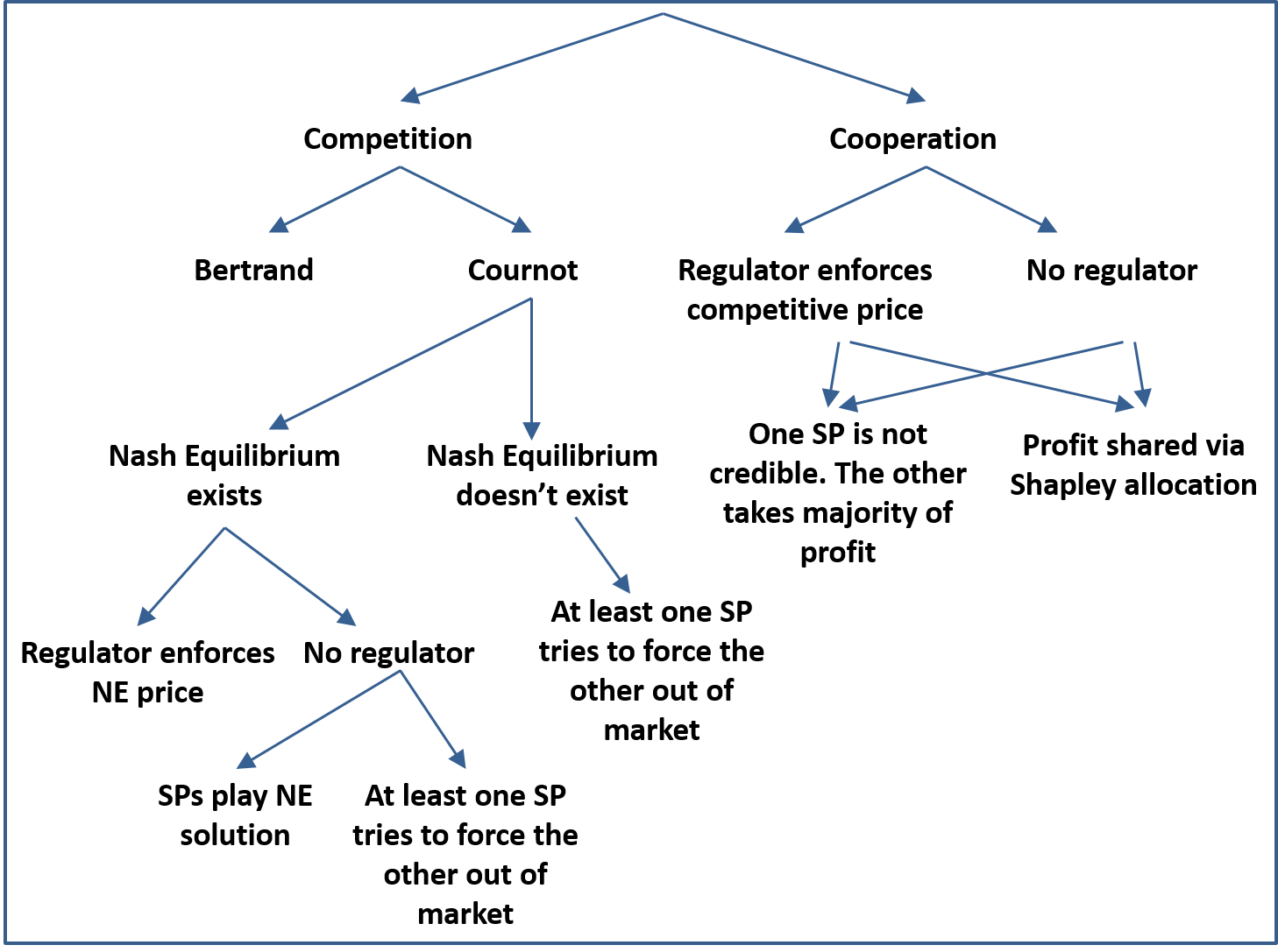
Figure 1: A schematic of the problem variants that we consider.

Much of the paper will focus on the dynamics and outcomes of a given competitive or collaborative scenario. Once those scenarios are established we can determine whether or not an SP would be better off entering into a sharing agreement or going it alone. However, there are many types of competitive or cooperative arrangements that each lead to different results for the SPs. We begin by giving a high-level description of the different regimes that can arise. These can be categorized in a hierachical manner as shown in Figure 1.

At a high level each SP needs to determine whether to compete with the other SP or whether to cooperate with it. For the case that SPs decide to compete there are two types of competition, a Bertrand game in which the SPs each offer their own price and the end users react accordingly, and a Cournot game in which each SP offers a certain capacity into the market and the market price is set accordingly.

The Cournot game admits a number of possible variations. First of all, depending on the problem parameters, there may or may not be a Nash equilibrium solution for the SPs. If there is a Nash equilibrium solution, then two situations can arise. In one of them there is a regulator that forces the end user price to be the one determined by the equilibrium solution. In the other there is no regulator and so each SP has to decided whether to play the equilibrium solution. The reason it might not do so is that depending on the cost parameters an SP might have the ability to force the other SP out of the market, i.e. it can play a strategy such that the other SP has no incentive to participate in the market. However, that is a risky strategy in that if both SPs try it then they could both be worse off than playing the equilibrium solution. We remark that the ability of one SP to drive the other out of the market arises solely because of the fixed component in the cost that leads to a non-convex cost function.

Our remaining analysis considers the situation when SPs cooperate and share their networks. For this case there are variants depending on whether there is a regulator that can enforce price limits. If there is a regulator then we assume that the end user price is forced to be the same as it would be if the SPs were competing according to a Cournot game. If there is no such regulator then we assume that the SPs can set prices as if the combined entity were a monopoly.

The remaining decisions refer to how the profits are shared when the two SPs cooperate. We assume that this depends on whether or not both SPs are credible players, i.e. whether or not they can legitimately offer service by themselves. If one SP deems that the other is not credible, then it would look to take the vast majority of the profit for itself. If both SPs can credibly offer service on their own, then we assume that profits in the sharing scenario are divided up according to appropriate schemes, (e.g. based on Shapley value).

1.2 Paper Organization

In Section 2 we define the models that we use throughout the paper and we outline the equations that define optimal demand and price for a monopolistic SP. In Section 3 we explore the dynamics for a prototypical example in a single geographic region. By starting with a concrete example we can better understand the fundamental dynamics at play rather than getting bogged down in the general equations (which can become somewhat complex). For this example we consider most of the regimes outlined in Figure 1.

In Section 4 we outline our results for the general case with much of the detailed analysis deferred to the Appendix. In particular, in Appendix A we present a more detailed study of the Cournot game in which the providers compete via deployed capacity. In particular, we derive the equations that characterize the Nash Equilibrium if it exists under our non-convex cost functions. We also examine the conditions under which one SP can drive the other out of the market. In Appendix B we determine the SP profits that arise when they enter into a sharing agreement. These profits are determined by how the combined profit is shared. This is calculated via two notions of Shapley value (one of which is based on the notion of “Shapley value with externalities”.) We also explore a regulatory framework that enforces Nash prices so that end users are not penalized in the sharing scenario. Lastly, we examine how an SP would approach a sharing agreement if it does not deem the other SP to be a credible competitor, i.e. if it does not believe the other SP has the cost structure to operate a network on its own.

In Appendix C we analyze the dynamics when the competitive setting is modeled as a Bertrand game. The analysis of the Bertrand game is in general simpler than the corresponding Cournot analysis. This is because in a Bertrand game the SP with the better cost structure always has the ability to drive the other SP out of the market. In addition to the basic Bertrand game we study a number of variants. In one of them the SPs are able to share network costs but they must still compete on price. In another variant only a subset of the end users are deemed to be price conscious.

In Appendix D we extend our analysis to a situation where a priori the SPs offer service in different geographic regions. This is an especially attractive situation for network sharing since it allows each SP to offer service over the entire market more rapidly.

1.3 Previous Work

The GSM Association wrote an influential report [4] examining the ways in which wireless infrastructure can be shared. This report describes some existing sharing agreements that are already in place and discusses the economic and regulatory implications. In [5], Janssen et al. discuss the statistical multiplexing gains that can be obtained by combining capacity in a network sharing arrangement. The economics of the Chinese tower sharing agreement mentioned earlier were analyzed by Deng et al. in [3]. Malanchini and Gruber studied small cell sharing in [7] and presented ways in which operators could still differentiate themselves (e.g. via power management) even if all network resources are shared. The papers [1, 6, 8, 13] discuss ways in which network sharing could be realized in practice. In particular, [6] discusses a technique known as “network slicing” in which the resource allocation algorithms at wireless basestations reserve a fraction of resources for each SP. The general economics literature contains many analyses of duopolies with various cost structures (e.g. [11]). However, to the best of our knowledge previous work has not considered Cournot competition for network providers under non-concave cost functions with fixed costs, and there has not been a comparison of how the dynamics under sharing compare to the competitive dynamics.

2 Cost Model

We consider two Service Providers (SPs) that we denote SP1 and SP2. We begin with a single geographical region in which both SPs operate. If SP $i$ serves demand of size $q_{i}$ then its cost is given by,

$$C_{i}(q_{i})=\left\{\begin{array}[]{cc}\alpha_{i}+\beta_{i}q_{i}&q_{i}>0\\ 0&q_{i}=0\end{array}\right.,$$

for some parameters $\alpha_{i}>0,\beta_{i}\geq 0$. The parameter $\alpha_{i}$ reflects a fixed cost, e.g. the cost of infrastructure such as buildings or spectrum, whereas the parameter $\beta_{i}$ reflects the cost of serving a unit of demand, e.g. the cost of deploying equipment.

The level of demand in the region (denoted $q$) is closely related to the price offered to the end users (denoted $p$). Our assumption is that all users in the region are price conscious. In particular, we assume that the market is elastic with elasticity coefficient ${\varepsilon}$ greater than 1, i.e. $q(p)=Qp^{-{\varepsilon}},$ for some parameter $Q$ (quantity sold at unit price). Roughly speaking this means that a 1% reduction in price results in an $({\varepsilon}-1)$% increase in revenue. We note that a change in the demand can reflect both a change in the number of end users creating that demand as well as a change in the demand per end user.

If SP $i$ serves demand $q_{i}>0$ at price $p_{i}$ then it receives a profit given by, $\Pi_{i}=q_{i}p_{i}-C_{i}(q_{i})=q_{i}p_{i}-(\alpha_{i}+\beta_{i}q_{i})$. We observe that the fixed cost $\alpha_{i}$ makes the cost function non-convex which distinguishes our analysis from many previous studies of network economics. In particular, if $\alpha_{i}\gg 0$ then SP $i$ may not wish to participate in the market because even as a monopolist it is unable to make a profit. If this decision is due to the capacity (Cournot) or price (Bertrand) offered by the other SP then we say that SP $i$ is driven out of the market.

Lemma 1.

Under monopoly pricing we have,

$$p^{mon} = {\varepsilon}\beta/({\varepsilon}-1),~{}~{}~{}~{}~{}~{}~{}~{}q^{mon}=Q({\varepsilon}\beta/({\varepsilon}-1))^{-{\varepsilon}}$$

$$\Pi^{mon} = Q\left((\frac{{\varepsilon}\beta}{{\varepsilon}-1})^{1-{\varepsilon}}-\beta(\frac{{\varepsilon}\beta}{{\varepsilon}-1})^{-{\varepsilon}}\right)-\alpha.$$

assuming that $\Pi^{mon}\geq 0$. (If not then the SP stays out of the market.)

The proof (which is standard) is given in Appendix E.

3 Narrative for a single example

We begin by exploring the dynamics for a prototypical example. In this way we can better understand the fundamental dynamics at play rather than getting bogged down in the general equations (which can become somewhat complex). In later sections we consider the general case (with much of the proofs and derivations deferred to the Appendix).

For our example the unit of demand is a PB and the unit of price is $1M. For these units the price elasticity function has parameters ${\varepsilon}=1.25$ and $Q=1000$. The per-unit capacity costs are $\beta_{1}=\$2.5M$ for SP1 and $\beta_{2}=\$2M$ for SP2 per petabyte (PB) of wireless capacity. The fixed capacity costs (representing the cost of participating in the market, e.g., for buying spectrum or building cell towers) are $\alpha_{1}=\$50M$ and $\alpha_{2}=\$100M$. For these parameters, the monopoly price, demand and profit for each operator is given by,

$$p_{1}^{mon}=\$12.5M, q_{1}^{mon}=42.6PB,~{}\Pi_{1}^{mon}=\$376M$$

$$p_{2}^{mon}=\$10.0M, q_{2}^{mon}=56.2PB,~{}\Pi_{2}^{mon}=\$350M$$

3.1 Network Sharing

We first examine the situation under network sharing. This is the easiest case to consider since we do not need to worry about the competitive dynamics between the SPs. In particular the SPs cooperate and use the lowest cost parameters that are available, i.e.

$$C^{coop}(q)=\alpha_{min}+\beta_{min}q,$$

where $\alpha_{min}=\min\{\alpha_{1},\alpha_{2}\}$ and $\beta_{min}=\min\{\beta_{1},\beta_{2}\}$. (See Figure 2 for a depiction of $C^{coop}(q)$ in comparison to $C_{1}(q)$ and $C_{2}(q)$.)

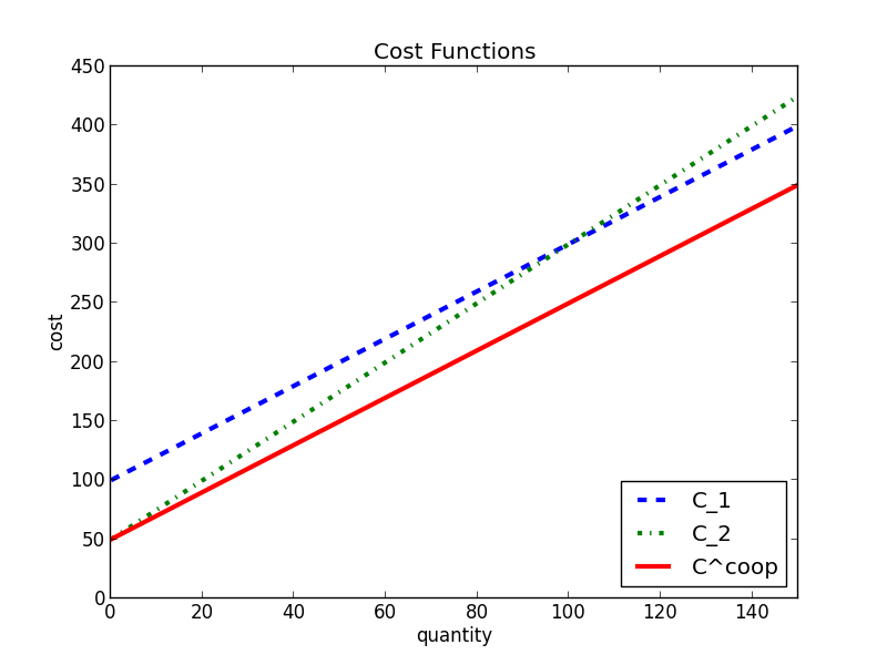
Figure 2: The cost function $C^{coop}(q)$ compared against $C_{1}(q)$ and $C_{2}(q)$.

We assume that the combined entity is able to use monopoly pricing. In this case the combined price, demand and profit for our running example is given by,

$$p^{coop}=\$10.0M,~{}q^{coop}=56.2PB,~{}\Pi^{coop}=\$400M$$

It remains to determine how the profit is split between the SPs. A natural way to do this is via the Shapley value which gives to SP $i$ its expected contribution to the coalition assuming that the SPs create the coalition in a random order. If we assume that the first SP to enter the coalition can utilize monopoly pricing then the profits are given by,

$$\Pi_{1}^{coop} = \frac{1}{2}(\Pi_{1}^{mon}+\Pi^{coop}-\Pi_{2}^{mon})=\$213M,$$

$$\Pi_{2}^{coop} = \frac{1}{2}(\Pi_{2}^{mon}+\Pi^{coop}-\Pi_{1}^{mon})=\$187M.$$

In order for an SP to determine whether network sharing is the best option, it needs to compare its profits under sharing with its profits for the case in which it competes with the other SP. As mentioned in Section 1, there are many notions of competition - a Cournot game in which the SPs offer capacity to the market and the market sets the price, and a Bertrand game in which the SPs directly offer prices to the market. We begin by examining the Cournot game and defer the corresponding analysis of the Bertrand game to the Appendix.

3.2 Cournot Game

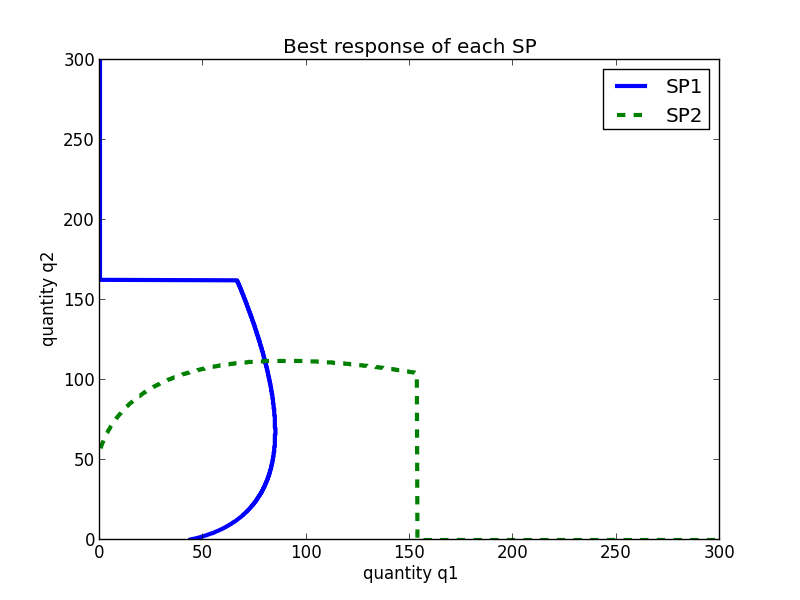
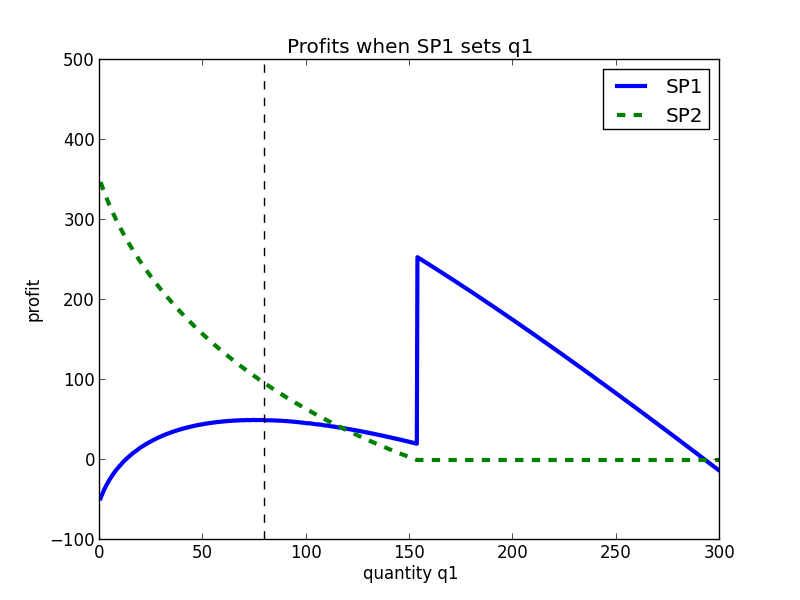
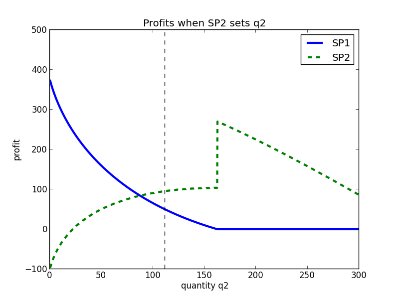
Figure 3: (Left) The best response for each SP given the actions of the other SP. (Middle) The profits of the two SPs as a function of $q1$ (assuming SP2 plays the best response). (Right) The profits of the two SPs as a function of $q2$ (assuming SP1 plays the best response). The vertical lines represent the Nash-Cournot solution ($q_{1}=80$, $q_{2}=112$).

In the Cournot game SP $i$ offers to serve demand $q_{i}$ and then the market determines a common price $p$ based on $q_{1}$ and $q_{2}$. In particular,

$$p=\left(\frac{q_{1}+q_{2}}{Q}\right)^{-1/{\varepsilon}}.$$

The main complication with the Cournot game in our setting is the presence of the $\alpha_{i}$ terms that introduce a discontinuity into the profit functions. If SP $i$ cannot generate a positive profit for any value $q_{i}>0$ then it will simply set $q_{i}=0$ and accept zero profit. In this case we say that SP $i$ is driven out of the market.

Figure 3 (left) illustrates the behavior of the Cournot game. The plot shows the best response for each SP, given the actions of the other SP. In particular, for any value $q_{1}>0$ (on the x-axis), the green dashed curve represents the value of $q_{2}$ (on the y-axis) that maximizes the profit of SP2 assuming that the action of SP1 is $q_{1}$.

The blue solid curve is similar and represents the best response for SP1 but with the axes flipped. In particular, for any value $q_{2}$ (on the y-axis), the blue curve represents the value of $q_{1}$ (on the x-axis) that maximizes the profit of SP1 assuming that the action of SP2 is $q_{2}$.

The crossing point of the curves at $(q_{1},q_{2})=(80,112)$ represents a Nash equilibrium. (A closed form expression for this equilbrium is presented in Appendix A.) In other words, if the action of SP1 is $q_{1}=80$ then the optimal action of SP2 is $q_{2}=112$ and if the action of SP2 is $q_{2}=112$ then the optimal action of SP1 is $q_{1}=80$. At this point the full set of quantity, price and profit values is given by,

$$p_{1}^{NC}=\$3.75M, q_{1}^{NC}=80PB,~{}\Pi_{1}^{NC}=\$50M$$

$$p_{2}^{NC}=\$3.75M, q_{2}^{NC}=112PB,~{}\Pi_{2}^{NC}=\$96M.$$

3.3 The impact of a regulator

As we will discuss shortly, the profits for each SP in the sharing scenario are significantly higher than they are in the competitive scenario. One main reason for this is that in the sharing case the combined entity is able to set a monopoly price. The profit increase therefore comes at the expense of the end users who have to pay higher prices. A regulator may deem this to be anti-competitive and as a result may impose an upper bound on the price that the combined entity can charge if the two SPs decide to share. A natural candidate for this upper bound is the price corresponding to the Nash Equilibrium that we computed in the previous section. Sharing can still be beneficial even if a regulator restricts the price because the combined entity can take advantage of the reduced cost function. (See Figure 2.) Moreover, in contrast to the full competitive case of Section 3.2 the SPs will share profits according to Shapley value and so we have,

$$p^{reg} = p_{1}^{NC}=\$3.75M,~{}q^{reg}=q_{1}^{NC}+q_{2}^{NC}=192PB,$$

$$\Pi^{reg} = p^{reg}q^{reg}-(\alpha_{min}+\beta_{min}q^{reg})=\$286M$$

This combined profit is shared via Shapley value and results in,

$$\Pi_{1}^{reg}=\$120M,~{}\Pi_{2}^{reg}=\$166M$$

3.4 Comparison of network sharing and the Cournot game

In the table in Figure 4 we summarize the price $p$ and the profits $\Pi_{1},\Pi_{2}$ for the case that the SPs compete according to the Nash Equilibrium of the Cournot game (the so-called Nash-Cournot solution), as well as the cases of network sharing with and without a regulator. We see that for the case of network sharing without a regulator, both SPs have significantly higher profit than in the Nash-Cournot solution but this is partly because they can charge a monopoly price to the end users. In the case that a regulator enforces an upper bound on price equal to the Nash-Cournot price, both SPs still obtain a higher profit with network sharing than in the Nash-Cournot solution. This latter effect comes from the fact that the SPs can share the cost of the network and utilize the cost parameters $\alpha_{min},\beta_{min}$ rather than $\alpha_{i},\beta_{i}$.

	price per PB, $p$	profits $(\Pi_{1},\Pi_{2})$
Nash-Cournot	3.75	(50, 96)
Sharing (no regulator)	10	(213,187)
Sharing (regulator)	3.75	(120,166)

Figure 4: The price $p$ and the SP profits $(\Pi_{1},\Pi_{2})$ due to the Nash-Cournot solution and the sharing scenarios. All quantities are in units of $1M.

3.5 Aggressive and submissive strategies

We now address the more complex dynamics that can arise due to the fact that $\alpha_{i}>0$. In particular, we ask whether the SPs will be motivated to conform to the Nash-Cournot solution or whether they might be tempted to deviate from that action. Note that both the blue and the green curves hit zero in Figure 3 (left), i.e. both SPs have the ability to drive the other one out of the market.

Figure 3 further illustrates why the temptation to deviate from the Nash equilibrium might exist. In particular, Figure 3 (middle) shows the profits of the two SPs given a fixed value of $q_{1}$. More precisely, for each value of $q_{1}$, the solid blue and dashed green curves show the profits of SP1 and SP2 respectively, if SP2 plays its optimal response. We see that there is a big discontinuity in the profit of SP1. At the point ($q_{1}=154$) at which SP1 drives SP2 out of the market, the optimal response of SP2 jumps from a non-zero value to zero. This means there is less capacity available which in turn drives up the price and hence the profit of SP1. Note however that it cannot claim the monopoly profit since it cannot reduce to the monopoly point $q_{1}=42.6$ without letting SP2 back into the market.

However, Figure 3 (right) shows that this process could work the other way round as well. In particular, this figure shows the profits of the two SPs given a fixed value of $q_{2}$. For each value of $q_{2}$, the solid blue and dashed green curves show the profits of SP1 and SP2 respectively, if SP1 plays its optimal response. This time we see a big jump in the profit of SP2 at the point at which it drives SP1 out of the market.

As a result, each SP could benefit if it sets its $q_{i}$ at a level that drives the other SP out of the market and the other SP acquiesces to being driven out. We can therefore model the game by assuming that the SPs have the following discrete choices.

• Nash-Cournot: In this case each SP assumes that the other SP will compete in the market in which case it makes sense to play the Nash equilibrium value.

• Aggression: An aggressive SP will play at a level that drives the other SP out of the market.

• Submission: A submissive SP will accept being shut out of the market (rather than fighting it and potentially taking a loss).

• Sharing: An SP can offer to enter a sharing arrangement with the other SP. However, the arrangement only goes into effect if both SPs agree to it. If both SPs do agree then we obtain the profits presented in Section 3.1 (that depend on whether or not a regulator caps the price $p$).

				Sharing	Sharing
(SP1 profit,SP2 profit)	Nash-Cournot	Aggression	Submission	(no regulator)	(regulator)
Nash-Cournot	(50, 96)	(-1,80)	(353,0)	NA	NA
Aggression	(9,-1)	(-48,-17)	(254,0)	NA	NA
Submission	(0,321)	(0,271)	(0,0)	NA	NA
Sharing (no regulator)	NA	NA	NA	(213,187)	NA
Sharing (regulator)	NA	NA	NA	NA	(120,166)

Figure 5: The profits $(\Pi_{1},\Pi_{2})$ due to the different strategy combinations. The rows represent the decisions for SP1 and the columns represent the decisions for SP2.

The table in Figure 5 shows the outcomes of the resulting game. The columns represent the decisions for SP1 and the rows represent the decisions for SP2. The entries have the form (SP1 profit, SP2 profit). The profits due to sharing are included in the bottom right corner of the table. Since sharing only takes place if both parties agree to share, there is no entry in the table if only one SP is sharing.

We remark that the italicized entries (where one SP plays the Nash-Cournot strategy and the other plays the Submission strategy) are not viable outcomes because the submissive SP would be better off playing the Nash-Cournot strategy as well. From the above we can conclude the following.

• Network sharing is better for both SPs than the Nash-Cournot solution

• If sharing does not take place then the Nash-Cournot solution is a unique Nash equilibrium since that is the only point at which both curves cross in Figure 3 (left).

• An SP might be tempted to deviate from the Nash-Cournot solution since if it aggressive then the best response of the other SP is to be submissive in which case the aggressive SP will do even better than sharing. (We note that this is not a Nash equilibrium since if one SP sets $q_{i}=0$ then the best response of the other SP is to set $q_{3-i}=q_{3-i}^{mon}$.)

• The downside of aggression is that if both SPs are aggressive then they both make negative profit and hence are worse off (as in standard games of chicken). Whether or not an SP will choose to be aggressive will largely depend on how it expects the other SP to react.

4 General Analysis

As mentioned earlier, most of our general analysis is deferred to the Appendices. However, in the following we state our main results for the case of network sharing compared with a Cournot competition.

For the case of sharing the combined price, demand and profit is given by,

$$p^{coop} = {\varepsilon}\beta_{min}/({\varepsilon}-1)$$

$$q^{coop} = Q({\varepsilon}\beta_{min}/({\varepsilon}-1))^{-{\varepsilon}}$$

$$\Pi^{coop} = p^{coop}q^{coop}-(\alpha_{min}+\beta_{min}q^{coop}),$$

where $\alpha_{min}=\min\{\alpha_{1},\alpha_{2}\}$ and $\beta_{min}=\min\{\beta_{1},\beta_{2}\}$. The profit is shared according to,

$$\Pi_{1}^{coop} = \frac{1}{2}(\Pi_{1}^{mon}+\Pi^{coop}-\Pi_{2}^{mon})$$ (1)

$$\Pi_{2}^{coop} = \frac{1}{2}(\Pi_{2}^{mon}+\Pi^{coop}-\Pi_{1}^{mon}),$$ (2)

where $\Pi^{mon}_{1},\Pi^{mon}_{2}$ are the monopoly profits for SPs 1 and 2 respectively.

For the case of the Cournot competition, for any given $q_{1},q_{2}$ the profits of the SPs are specified:

$$\Pi_{1}(q_{1},q_{2}) = \left(\frac{Q}{q_{1}+q_{2}}\right)^{1/\varepsilon}q_{1}-\alpha_{1}-\beta_{1}q_{1}$$ (3)

$$\Pi_{2}(q_{1},q_{2}) = \left(\frac{Q}{q_{1}+q_{2}}\right)^{1/\varepsilon}q_{2}-\alpha_{2}-\beta_{2}q_{2}$$ (4)

We first need to calculate the best response function for each provider. If SP2 offers to serve demand $q_{2}$, we show that the best response of SP1 is to set $q_{1}$ so that $q_{1}/q_{2}$ is the solution to the equation,

$$(z+1)^{1+\frac{1}{\varepsilon}}=Az+B,$$

where $A=(1-\frac{1}{\varepsilon})(Q/(q_{2}\beta_{1}^{\varepsilon}))^{1/\varepsilon}$ and $B=(Q/(q_{2}\beta_{1}^{\varepsilon}))^{1/\varepsilon}$, assuming that this leads to a positive profit. We use $\hat{q}_{1}(q_{2})$ to denote this solution for any fixed value of $q_{2}$. The best response function for SP2 can be defined analogously.

Now that the best response functions are in place, we can calculate the Nash-Cournot solution which is given by,

$$t = \frac{1-\beta_{2}/\beta_{1}(1-1/\varepsilon)}{\beta_{2}/\beta_{1}-(1-1/\varepsilon)}$$

$$q_{1}^{*} = Q\left(\frac{1+t(1-\frac{1}{\varepsilon})}{\beta_{2}(1+t)^{1+\frac{1}{\varepsilon}}}\right)^{\varepsilon}$$

$$q_{2}^{*} = Q\left(\frac{\frac{1}{t}(1-\frac{1}{\varepsilon})+1}{\beta_{1}(\frac{1}{t}+1)^{1+\frac{1}{\varepsilon}}}\right)^{\varepsilon}$$

(We remark that in some cases this Nash Equilibrium may not exist if either $q^{*}_{1}$ or $q^{*}_{2}$ is negative or if either of the corresponding profits are negative.)

As we saw in our running example, even if the Nash Equilibrium does exist an SP may have an incentive to not play the Nash equilibrium solution but instead try to drive the other SP out of the market. If SP1 wishes to be aggressive in this way then it sets $q_{1}=q^{\prime}_{1}$, where

$$q^{\prime}_{1}=\arg\max_{q_{1}:\Pi_{2}(q_{1},\hat{q}_{2}(q_{1}))\leq 0}\{\Pi_{1}(q_{1},0)\}.$$

(A similar expression can be derived for the aggressive strategy of SP2.) Since for the submission strategy SP $i$ simply sets $q_{i}=0$, we have now defined the values of $q_{1},q_{2}$ for the cases of Nash-Cournot, Aggression and Submission. For any problem instance we can then utilize the profit functions of Equations (3) and (4) for each possible pair of strategies and combine the results with the profits for sharing (given in Equations (1) and (2) in order to obtain a table of the form shown in Figure 5.

5 Conclusions

In this paper we have presented a model to illustrate the options facing two Service Providers who are deciding whether or not to share network infrastructure. Our cost function has a fixed component and hence is non-convex. We presented a taxonomy of problem variants and derived the profit for each SP both in the case that they share infrastructure as well as the case that they are competitors. For the latter case the dynamics are complicated because the fixed cost function gives an SP the option to be aggressive and try to drive the other SP out of the market. For our running example the profit to each SP in the case of sharing is significantly higher than when they compete fairly according to a Nash Equilibrium, and the profit is comparable to the case in which the SP is aggressive and the other SP is submissive. For this example each SP would likely consider sharing to be a better option since even if it plays agressively in a competitive setting there is no way to ensure that the other SP would not try to be agressive as well.

A number of problems remain. In particular we would like to determine how the dynamics would change if the two SPs only share a portion of the network infrastructure. We would also like to incorporate roaming agreements into the model since they represent a “halfway” point between total competition and full cooperation.

Appendix A Detailed analysis of the Cournot competition

We now present our more detailed general analysis. We start with the competitive setting governed by the Cournot game, in the which SPs compete by deciding how much demand they wish to serve. Our analysis is more complex than the textbook Cournot analysis since the presence of the non-zero $\alpha_{i}$ parameters means that each SP is faced with a decision regarding whether or not to compete.

In the Cournot setting the price is determined by the aggregate demand, i.e.

$$p^{NC}=\left(\frac{q_{1}^{NC}+q_{2}^{NC}}{Q}\right)^{-1/{\varepsilon}},$$

We first consider a relaxation of the game in which the $q_{i}$ values can be negative and the profit is always given by $\Pi_{i}=q_{i}p_{i}-(\alpha_{i}+\beta_{i}q_{i})$, regardless of whether or not it is positive. In this case we assume that the quantities $q_{1}^{NC}$, $q_{2}^{NC}$ are chosen so that they form a Nash equilibrium with respect to the SP profits. Hence we wish to find a solution for which $\partial\Pi_{i}/\partial q_{i}=0$ for $i=1,2$.

Theorem 1.

When the SPs compete on quantity in the relaxed Nash-Cournot game, the solution is given by,

$$t = \frac{1-\beta_{2}/\beta_{1}(1-1/\varepsilon)}{\beta_{2}/\beta_{1}-(1-1/\varepsilon)}$$

$$q_{1}^{*} = Q\left(\frac{1+t(1-\frac{1}{\varepsilon})}{\beta_{2}(1+t)^{1+\frac{1}{\varepsilon}}}\right)^{\varepsilon}$$

$$q_{2}^{*} = Q\left(\frac{\frac{1}{t}(1-\frac{1}{\varepsilon})+1}{\beta_{1}(\frac{1}{t}+1)^{1+\frac{1}{\varepsilon}}}\right)^{\varepsilon}$$

$$p^{NC} = \left(\frac{q_{1}^{*}+q_{2}^{*}}{Q}\right)^{-1/\varepsilon}$$

$$\Pi_{1}^{NC} = \Pi_{1}(q_{1}^{*},q_{2}^{*})=\left(\frac{Q}{q_{1}^{*}+q_{2}^{*}}\right)^{1/\varepsilon}q_{1}^{*}-\alpha_{1}-\beta_{1}q_{1}^{*}$$

$$\Pi_{2}^{NC} = \Pi_{2}(q_{1}^{*},q_{2}^{*})=\left(\frac{Q}{q_{1}^{*}+q_{2}^{*}}\right)^{1/\varepsilon}q_{2}^{*}-\alpha_{2}-\beta_{2}q_{2}^{*}$$

Proof.

For ease of notation we drop the superscript $NC$ in this analysis. Define $S:=q_{1}+q_{2}$. The solution is given by:

$$\partial\Pi_{1}(q_{1},q_{2})/\partial q_{1}=0\,,$$ (5)

that is,

$$S^{-(1+(1/\varepsilon))}(S-q_{1}/\varepsilon)=\beta_{1}Q^{-1/\varepsilon}\,,$$ (6)

and

$$\partial\Pi_{2}(q_{1},q_{2})/\partial q_{2}=0\,,$$ (7)

that is,

$$S^{-(1+(1/\varepsilon))}(S-q_{2}/\varepsilon)=\beta_{2}Q^{-1/\varepsilon}\,.$$ (8)

For any fixed $q_{2}$, we can solve Equation 6 according to:

$$(q_{1}+q_{2})^{-(1+\frac{1}{\varepsilon})}(q_{1}(1-\frac{1}{\varepsilon})+q_{2}) = \beta_{1}Q^{-\frac{1}{\varepsilon}}$$

$$\Leftrightarrow(q_{1}+q_{2})^{1+\varepsilon}(q_{1}(1-\frac{1}{\varepsilon})+q_{2})^{-\varepsilon} = \beta_{1}^{-\varepsilon}Q$$

$$\Leftrightarrow q_{2}^{1+\varepsilon}(\frac{q_{1}}{q_{2}}+1)^{1+\varepsilon}q_{2}^{-\varepsilon}(\frac{q_{1}}{q_{2}}(1-\frac{1}{\varepsilon})+1)^{-\varepsilon} = \beta_{1}^{-\varepsilon}Q$$

$$\Leftrightarrow\left(\frac{(\frac{q_{1}}{q_{2}}+1)^{1+\frac{1}{\varepsilon}}}{\frac{q_{1}}{q_{2}}(1-\frac{1}{\varepsilon})+1}\right) = \left(\frac{Q}{q_{2}\beta_{1}^{\varepsilon}}\right)^{1/\varepsilon}.$$

In other words, $q_{1}/q_{2}$ is the solution to the equation,

$$(z+1)^{1+\frac{1}{\varepsilon}}=Az+B,$$

where $A=(1-\frac{1}{\varepsilon})(Q/(q_{2}\beta_{1}^{\varepsilon}))^{1/\varepsilon}$ and $B=(Q/(q_{2}\beta_{1}^{\varepsilon}))^{1/\varepsilon}$. We use $\hat{q}_{1}(q_{2})$ to denote this solution for any fixed value of $q_{2}$.

For any fixed $q_{1}$, we can solve Equation 8 according to:

$$(q_{1}+q_{2})^{-(1+\frac{1}{\varepsilon})}(q_{1}+q_{2}(1-\frac{1}{\varepsilon})) = \beta_{2}Q^{-\frac{1}{\varepsilon}}$$

$$\Leftrightarrow(q_{1}+q_{2})^{1+\varepsilon}(q_{1}+q_{2}(1-\frac{1}{\varepsilon}))^{-\varepsilon} = \beta_{2}^{-\varepsilon}Q$$

$$\Leftrightarrow q_{1}^{1+\varepsilon}(1+\frac{q_{2}}{q_{1}})^{1+\varepsilon}q_{1}^{-\varepsilon}(1+\frac{q_{2}}{q_{1}}(1-\frac{1}{\varepsilon}))^{-\varepsilon} = \beta_{2}^{-\varepsilon}Q$$

$$\Leftrightarrow\left(\frac{(1+\frac{q_{2}}{q_{1}})^{1+\frac{1}{\varepsilon}}}{1+\frac{q_{2}}{q_{1}}(1-\frac{1}{\varepsilon})}\right) = \left(\frac{Q}{q_{1}\beta_{2}^{\varepsilon}}\right)^{1/\varepsilon}.$$

In other words, $q_{2}/q_{1}$ is the unique positive solution to the equation,

$$(1+z)^{1+\frac{1}{\varepsilon}}=Az+B,$$

where $A=(1-\frac{1}{\varepsilon})(Q/(q_{1}\beta_{2}^{\varepsilon}))^{1/\varepsilon}$ and $B=(Q/(q_{1}\beta_{2}^{\varepsilon}))^{1/\varepsilon}$. We use $\hat{q}_{2}(q_{1})$ to denote this solution for any fixed value of $q_{1}$.

Suppose we now want to solve both Equations 6 and 8 simultaneously. By dividing the two equations we have

$$\beta_{2}(S-\frac{q_{1}}{\varepsilon}) = \beta_{1}(S-\frac{q_{2}}{\varepsilon})$$

$$\Rightarrow\frac{\beta_{2}}{\beta_{1}}(q_{1}(1-\frac{1}{\varepsilon})+q_{2}) = q_{1}+q_{2}(1-\frac{1}{\varepsilon})$$

$$\Rightarrow(1-\frac{\beta_{2}}{\beta_{1}}(1-\frac{1}{\varepsilon}))q_{1} = (\frac{\beta_{2}}{\beta_{1}}-(1-\frac{1}{\varepsilon}))q_{2}.$$

For $\beta_{2}/\beta_{1}\neq(1-1/\varepsilon)$, we have

$$q_{2}=\frac{1-(\beta_{2}/\beta_{1})(1-1/\varepsilon)}{\beta_{2}/\beta_{1}-(1-1/\varepsilon)}q_{1}\,,$$ (9)

and so $t:=q_{2}/q_{1}=\frac{1-\beta_{2}/\beta_{1}(1-1/\varepsilon)}{\beta_{2}/\beta_{1}-(1-1/\varepsilon)}$, which can be calculated by knowing the parameters $\varepsilon$, $\beta_{1},\beta_{2}$. If we let $(q_{1}^{*},q_{2}^{*})$ be the solution to the simultaneous equations then it follows,

$$q_{1}^{*}=Q\left(\frac{1+t(1-\frac{1}{\varepsilon})}{\beta_{2}(1+t)^{1+\frac{1}{\varepsilon}}}\right)^{\varepsilon}\,,$$ (10)

and

$$q_{2}^{*}=Q\left(\frac{\frac{1}{t}(1-\frac{1}{\varepsilon})+1}{\beta_{1}(\frac{1}{t}+1)^{1+\frac{1}{\varepsilon}}}\right)^{\varepsilon}\,.$$ (11)

(The ratio $q_{2}^{*}/q_{1}^{*}$ indeed equals $t$). The corresponding profits are given by,

$$\Pi_{1}^{NC}:=\Pi_{1}(q_{1}^{*},q_{2}^{*})=\left(\frac{Q}{q_{1}^{*}+q_{2}^{*}}\right)^{1/\varepsilon}q_{1}^{*}-\alpha_{1}-\beta_{1}q_{1}^{*}\,,$$ (12)

and

$$\Pi_{2}^{NC}:=\Pi_{2}(q_{1}^{*},q_{2}^{*})=\left(\frac{Q}{q_{1}^{*}+q_{2}^{*}}\right)^{1/\varepsilon}q_{2}^{*}-\alpha_{2}-\beta_{2}q_{2}^{*}\,.$$ (13)

∎

We now consider the real, i.e. non-relaxed problem and derive the conditions under which the above Nash equilibrium is a valid solution. This is the case if $q_{1}^{*}$, $q_{2}^{*}$, $\Pi_{1}(q_{1}^{*},q_{2}^{*})$ and $\Pi_{2}(q_{1}^{*},q_{2}^{*})$ are all non-negative. From the above analysis we immediately have,

Lemma 2.

The pair $(q_{1}^{*},q_{2}^{*})$ is a viable solution to the original problem if and only if,

$$(1-1/\varepsilon) \leq \min\{\beta_{1}/\beta_{2},\beta_{2}/\beta_{1}\},$$

$$\alpha_{1} \leq \left(\frac{Q}{q_{1}^{*}+q_{2}^{*}}\right)^{1/\varepsilon}q_{1}^{*}-\beta_{1}q_{1}^{*},$$

$$\alpha_{2} \leq \left(\frac{Q}{q_{1}^{*}+q_{2}^{*}}\right)^{1/\varepsilon}q_{2}^{*}-\beta_{2}q_{2}^{*}.$$

Suppose that the conditions of Lemma 2 do not hold. Note that due to the unimodal nature of the profit curve, if $q_{i}^{*}$ is negative then SP $i$ would be better off setting $q_{i}=0$. Also, if $\Pi_{i}^{NC}$ is negative then SP $i$ would be better off setting $q_{i}=0$. In each of these cases we say that SP $i$ is driven out of the market.

However, as we first discussed in Section 3.5, even if the Nash equilibrium is a viable solution an SP may still be incentivized to try and drive the other SP out of the market. other SP out of the market and so we now investigate that situation in detail. In particular let,

$$q^{\prime}_{1}=\arg\max_{q_{1}:\Pi_{2}(q_{1},\hat{q}_{2}(q_{1}))\leq 0}\{\Pi_{1}(q_{1},0)\}.$$

In other words, let $q^{\prime}_{1}$ be the value of $q_{1}$ that maximizes the profit of SP1 assuming that it can drive SP2 out of the market even if SP2 gives the best response. Similarly let,

$$q^{\prime}_{2}=\arg\max_{q_{2}:\Pi_{1}(\hat{q}_{1}(q_{2}),q_{2})\leq 0}\{\Pi_{2}(0,q_{2})\}.$$

With these formulas in place, SP1 chooses from the following three options.

• Option 1 (Nash-Cournot). Playing value $q_{1}^{*}$ under the assumption that SP2 plays value $q_{2}^{*}$. This option is viable if all of the quantities, $q_{1}^{*}$, $q_{2}^{*}$, $\Pi_{1}(q_{1}^{*},q_{2}^{*})$ and $\Pi_{2}(q_{1}^{*},q_{2}^{*})$ are non-negative, i.e. if the conditions of Lemma 2 hold.

• Option 2 (Aggression). Playing value $q^{\prime}_{1}$ with the expectation that SP2 plays value $0$, (i.e. it does not participate in the market).

• Option 3 (Submission). Playing value $0$, i.e. not participating in the market.

SP2 is faced with an analogous set of options and so we obtain the following profit table in Figure 6 that is a general version of the first three columns and rows in Figure 5.

	Nash-Cournot	Aggression	Submission
Nash-Cournot	$(\Pi_{1}(q^{*}_{1},q^{*}_{2}),\Pi_{2}(q^{*}_{1},q^{*}_{2}))$	$(\Pi_{1}(q^{*}_{1},q^{\prime}_{2}),\Pi_{2}(q^{*}_{1},q^{\prime}_{2}))$	$(\Pi_{1}(q^{*}_{1},0),0)$
Aggression	$(\Pi_{1}(q^{\prime}_{1},q^{*}_{2}),\Pi_{2}(q^{\prime}_{1},q^{*}_{2})$	$(\Pi_{1}(q^{\prime}_{1},q^{\prime}_{2}),\Pi_{2}(q^{\prime}_{1},q^{\prime}_{2}))$	$(\Pi_{1}(q^{\prime}_{1},0),0)$
Submission	$(0,\Pi_{2}(0,q^{*}_{2}))$	$(0,\Pi_{2}(0,q^{\prime}_{2}))$	$(0,0)$

Figure 6: The profits $(\Pi_{1},\Pi_{2})$ due to the different strategy combinations. The rows represent the decisions for SP1 and the columns represent the decisions for SP2.

Appendix B Network Sharing

We now examine the situation under network sharing. In this case the SPs cooperate and use the lowest cost parameters that are available, i.e.

$$C^{coop}(q)=\alpha_{min}+\beta_{min}q,$$

where $\alpha_{min}=\min\{\alpha_{1},\alpha_{2}\}$ and $\beta_{min}=\min\{\beta_{1},\beta_{2}\}$.

We first assume that the combined entity is able to use monopoly pricing. In this case the combined price, demand and profit is given by,

$$p^{coop} = {\varepsilon}\beta_{min}/({\varepsilon}-1)$$

$$q^{coop} = Q({\varepsilon}\beta_{min}/({\varepsilon}-1))^{-{\varepsilon}}$$

$$\Pi^{coop} = p^{coop}q^{coop}-(\alpha_{min}+\beta_{min}q^{coop})$$

It remains to determine how the profit is split between the SPs. A natural way to do this is via the Shapley value which gives to SP $i$ its expected contribution to the coalition assuming that the SPs create the coalition in a random order. There are two ways to calculate this number depending on whether we incorporate externalities [9, 10] from outside the coalition. More precisely, when SP $i$ is the first member of the coalition, we can either assume that it can utilize monopoly pricing or we can assume that it still has to compete against the other SP according to the Nash-Cournot game. The former case might be more appropriate in a rural setting in which an SP that enters the market late is unlikely to participate in the market unless it can share. The latter case might be more appropriate in an urban situation in which both SPs feel compelled to enter the market regardless of whether or not they can share. In the first case we get,

$$\Pi_{1}^{coop} = \frac{1}{2}(\Pi_{1}^{mon}+\Pi^{coop}-\Pi_{2}^{mon})$$

$$\Pi_{2}^{coop} = \frac{1}{2}(\Pi_{2}^{mon}+\Pi^{coop}-\Pi_{1}^{mon}).$$

In the latter case we get,

$$\Pi_{1}^{coop} = \frac{1}{2}(\Pi_{1}^{NC}+\Pi^{coop}-\Pi_{2}^{NC})$$

$$\Pi_{2}^{coop} = \frac{1}{2}(\Pi_{2}^{NC}+\Pi^{coop}-\Pi_{1}^{NC}).$$

(In Figure 1 these cases make up the “Cooperation$\rightarrow$No regulator$\rightarrow$Profit shared via Shapley allocation” branches.)

From a regulator’s point of view, the downside of sharing under monopoly pricing is that the price is significantly higher than the competitive case. We now look at an alternative framework in which the price is restricted by a regulator to be the same as in the Nash-Cournot game. In this setting the solution becomes,

$$p^{coop} = p^{NC}$$

$$q^{coop} = Q(p^{NC})^{-{\varepsilon}}$$

$$\Pi^{coop} = q^{coop}p^{coop}-(\alpha_{min}+\beta_{min}q^{coop}).$$

Now when we consider the Shapley value without externalities, it only makes sense to assume that the price is constrained to be the regulated price, regardless of the size of the coalition. Hence in all cases the price and demand are the same and so the only difference between the coalitions is the cost.

$$\Pi_{1}^{coop} = \frac{1}{2}(q^{coop}p^{coop}-(\alpha_{1}+\alpha_{min}-\alpha_{2})$$

$$-(\beta_{1}+\beta_{min}-\beta_{2})q^{coop})$$

$$\Pi_{2}^{coop} = \frac{1}{2}(q^{coop}p^{coop}-(\alpha_{2}+\alpha_{min}-\alpha_{1})$$

$$-(\beta_{2}+\beta_{min}-\beta_{1})q^{coop})$$

For the Shapley value with externalities we have,

$$\Pi_{1}^{coop} = \frac{1}{2}((q_{1}^{NC}+q^{coop}-q_{2}^{NC})p^{coop}-(\alpha_{1}+\alpha_{min}-\alpha_{2})$$

$$-(\beta_{1}q_{1}^{NC}+\beta_{min}q^{coop}-\beta_{2}q_{2}^{NC}))$$

$$\Pi_{2}^{coop} = \frac{1}{2}((q_{2}^{NC}+q^{coop}-q_{1}^{NC})p^{coop}-(\alpha_{2}+\alpha_{min}-\alpha_{1})$$

$$-(\beta_{2}q_{2}^{NC}+\beta_{min}q^{coop}-\beta_{1}q_{1}^{NC}))$$

Appendix C Price competition and breaking the “Bertrand curse”

The results of Appendix A were for the Cournot notion of competition by offered capacity. Each SP decides to serve demand $q_{i}$ and then the price is determined by the total capacity $q_{1}+q_{2}$. The main alternative notion of competition is a Bertrand competition in which the providers offer a price to the market. In this section we examine how a price-based competition operates under various notions of price-sensitivity for the end users. We start with the outcome of our running example for the case of a Bertrand competition.

C.1 Bertrand analysis for the running example.

Recall our example from Section 3 in which the price elasticity function has parameters ${\varepsilon}=1.25$ and $Q=1000$. The per-unit capacity costs are $\beta_{1}=\$2.5M$ for SP1 and $\beta_{2}=\$2M$ for SP2 and the fixed capacity costs are $\alpha_{1}=\$50M$ and $\alpha_{2}=\$100M$.

We now consider the dynamics of this example under the simplest type of Bertrand game. If the SPs offer different prices then all the demand goes to the one with the lowest price. If the two SPs offer the same price then the demand is split between them. The value of the lowest price determines the amount of demand in the market.

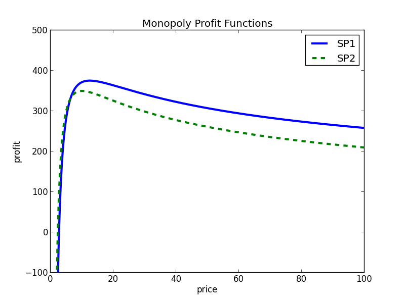
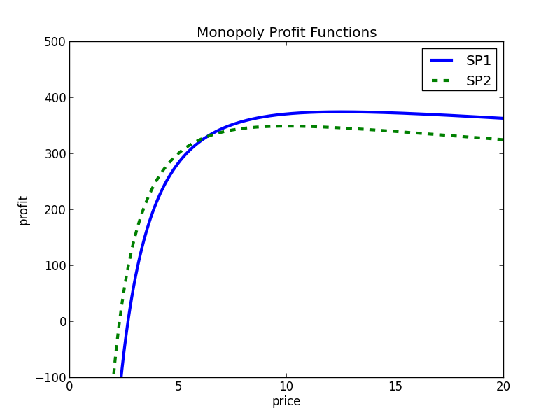
Figure 7: (Left) The profit for the two SPs as a function of the price $p$. Here $\alpha_{1}=\$50M$, $\beta_{1}=\$2.5M$, $\alpha_{2}=\$100M$ and $\beta_{2}=\$2M$. (Right) A blown up version of the figure.

In Figure 7 (left) we show the monopoly profit function for these parameters as a function of price, $p$. We denote these functions by $\Pi_{1}^{mon}(p)$ and $\Pi_{2}^{mon}(p)$. Figure 7 (right) shows a blown up version of the figure.

We see from the figure that $\Pi_{1}^{mon}(p)\leq 0$ for $p\leq 2.68$ and $\Pi_{2}^{mon}(p)\leq 0$ for $p\leq 2.28$. Hence if $p_{1}\geq 2.68$ then SP2 can always claim all the demand and gain a positive profit by setting $p_{2}=\frac{1}{2}(p_{1}+2.28)$. As a result, a natural strategy for SP2 is to set $p_{2}$ slightly under 2.68 (e.g. at $2.67$). This effectively drives SP1 out of the market since there is no setting for $p_{1}$ that would allow it to claim nonzero demand and make a positive profit. The resulting solution is:

$$p_{1}=\$2.68M, q_{1}=0PB,~{}\Pi_{1}=\$0M$$

$$p_{2}=\$2.67M, q_{2}=293PB,~{}\Pi_{2}=\$96.3M.$$

We now comment on the difference between the Bertrand and Cournot results and how they compare to the sharing scenario.

• In the Cournot game, each SP has the ability to drive the other out of the market. In the Bertrand game, only SP2 can do that. The reason for this asymmetry in the Bertrand game is that SP2 has a lower variable cost, i.e. $\beta_{2}<\beta_{1}$. (For example, this might be due to SP2 having a lower cost for deploying capacity.) Hence SP2 can make a profit at a lower price than SP1.

• If competition is modeled according to a Bertrand game, SP2 is better off sharing with SP1 than driving SP1 out of the market. In contrast, if competition is modeled according to a Cournot game, both SPs can do better than sharing if they are able to drive the other SP out of the market.

• With the Bertrand game, if SP2 drives SP1 out of the market, there is no action of SP1 that would cause SP2 to have a negative profit. In contrast, in the Cournot game if one SP is aggressive and tries to drive the other out of the market, the aggressive SP is in danger of making a negative profit if the other SP refuses to be submissive and also decides to act aggressively.

We now provide a general analysis of the Bertrand game. In Section C.2 we examine the basic Bertrand model and then in Section C.3 we show how the results change when not all users are price sensitive. This type of model has been considered as one way of breaking the “Bertrand curse” which occurs when both providers have the same costs and so neither can achieve a profit. In Section C.4 we consider another extension of the basic model that is motivated by potential actions of a regulator. In this extension (that is a combination of the sharing model and the Bertrand game) the SPs are allowed to share costs but the regulator enforces that they must still compete on price.

C.2 Bertrand model 1: all end users are price sensitive

In this simplest case we assume that all demand goes to the SP that offers the lowest price and if both SPs offer the same price then the demand is split between them. Suppose that the $\alpha_{i},\beta_{i}$ parameters are fixed.

• $\alpha_{i}\geq Q(({\varepsilon}\beta_{i}/({\varepsilon}-1))^{1-{\varepsilon}}-\beta_{i}^{1-{\varepsilon}}({\varepsilon}/({\varepsilon}-1))^{-{\varepsilon}})$ for $i=1,2$. In this case a Nash equilibrium is for both SPs to stay out of the market and keep a profit of zero. This is because neither can attain a positive profit, even if they can act as a monopoly.

• If the above condition does not hold for SP $i$, let $\underline{p}_{i}=\min\{p:Qp^{1-{\varepsilon}}-(\alpha_{i}+\beta_{i}Qp^{-{\varepsilon}})\geq 0\}$ and let $\bar{p}_{i}=\max\{p:Qp^{1-{\varepsilon}}-(\alpha_{i}+\beta_{i}Qp^{-{\varepsilon}})\geq 0\}$. Suppose without loss of generality that $\underline{p}_{1}\geq\underline{p}_{2}$. If $\bar{p}_{2}\leq\underline{p}_{1}$ then a Nash equilibrium is for SP2 to set price $p_{2}=p_{2}^{mon}$ and for SP1 to stay out of the market.

• If $\bar{p}_{2}>\underline{p}_{1}$ and $\underline{p}_{2}<\underline{p}_{1}$ (i.e. with strict inequality) then a natural solution is for SP2 to set price $p_{2}=\min{p_{2}^{mon},\underline{p}_{1}}$ and for SP1 to stay out of the market. Note that this is not a Nash equilibrium in the strict sense since if SP1 does not participate then the optimal action of SP2 is to set its price to its monopoly price. However, if SP2 did that then SP1 could potentially get back into the market. Hence a more natural course of action for SP2 is to set its price to the best price that keeps SP1 out of the market.

• If $\underline{p}_{2}=\underline{p}_{1}$ then it is not hard to see that the only Nash equilibrium is for both SPs to set price $p_{i}=\underline{p}_{i}$ which gives them zero profit. This is an example of the so-called Bertrand curse in which either one provider is driven completely out of the market or else both providers make zero profit.

C.3 Bertrand model 2: not all end users are price sensitive

The Bertrand curse is generally viewed as a an undesirable state of affairs and so there has been much research on methods to avoid it. We now consider how our results change in a framework of Bagwell and Lee [2] that was inspired by earlier work Varian [14]. In this model we assume that a fraction $I$ of the end users (the “informed” users) are price sensitive and a fraction $U=1-I$ (the “uninformed” users) are price insensitive. However, each end user still generates demand based on price according to the price elasticity function. Let,

$$\Pi_{i}^{+}(p) = (I+\frac{U}{2})pq(p)-(\alpha_{i}+\beta_{i}q(p))$$

$$\Pi_{i}^{-}(p) = \frac{U}{2}pq(p)-(\alpha_{i}+\beta_{i}q(p))$$

In other words, $\Pi_{i}^{+}(p)$ is the profit function when SP $i$ has the low price and $\Pi_{i}^{-}(p)$ is the profit function when SP $i$ has the high price. Let $[\underline{p}^{-}_{i},\bar{p}^{-}_{i}]$ be the price range on which $\Pi^{-}_{i}$ is non-negative and let $[\underline{p}^{+}_{i},\bar{p}^{+}_{i}]$ be the price range on which $\Pi^{+}_{i}$ is non-negative. We assume without loss of generality that $\underline{p}^{+}_{2}\leq\underline{p}^{+}_{1}$.

For this case we claim that the following is a stable solution. SP1 sets its price $p_{1}$ so as to maximize $\Pi^{-}_{1}$. Now let $\hat{p}_{1}\leq p_{1}$ be such that $\Pi^{+}_{1}(\hat{p}_{1})=\Pi^{-}_{1}(p_{1})$. SP2 sets its price $p_{2}=\min\{\hat{p}_{1},\arg\max\Pi^{+}_{2}(p)\}$.

We show that this solution is a stable solution in the following sense. First of all, given the price offered by SP2, SP1 cannot improve its profit with any other price. Hence it satisfies the property of a Nash equilbrium from the perspective of SP1. It does not satsify the property of a Nash equilibrim from the perspective of SP2 since SP2 could potentially increase its profit if SP1 keeps its price fixed. However, if SP2 did that then SP1 could choose a new price in which SP1 does better and SP2 does worse. Another way to look at this is that these prices form a subgame perfect Nash equilibrium for the Stackelberg game in which SP2 sets its price first and then SP1 follows.

C.4 Sharing on cost with price competition

When considering the benefits of sharing in the context of a Bertrand competition, one model of sharing would be exactly as was considered before in the context of a Nash Cournot competition. The service providers provide capacity based on the minimum of their costs and then calculate a monopoly price with respect to those costs. The above notion of a Bertrand competition with insensitive users gives rise to another notion of sharing that might be more appealing to a regulator. In particular, the SPs are allowed to cooperate on cost when building capacity. However, when offering service to end users they must still compete on price. This gives rise to a Bertrand competition in which each SP has parameters $\alpha_{\min}=\min\{\alpha_{1},\alpha_{2}\}$ and $\beta_{\min}=\min\{\beta_{1},\beta_{2}\}$. In the case of a Bertrand competition in which all users are price sensitive, both SPs would offer a price $p=\beta_{\min}$ and so neither would generate a profit. However, for the case in which some users are price insensitive, there is a stable situation as described above in which one SP offers a low price in order to get all the price sensitive users while the other one offers a high price in order to get all the price insensitive users.

Appendix D Multiple Geographic Regions

One of the main reasons that regulators allow network sharing even though it leads to loss of competition is that it allows service providers to more quickly offer service over a large geographic region. In order to investigate this phenomenon, we now show how our analysis extends when it is not the case that both SPs can offer service by themselves over the entire market. For this analysis we focus on the specific SP cost parameters given in Section 3.

We consider two scenarios, both of which have two regions W and E. In the first scenario SP1 can provide service in region W (with its $\alpha$ value halved to represent fixed costs in one region only), and SP2 can provide service in region E (with its $\alpha$ value also halved). There are three types of user, W, E and WE. WE users need a service provider that can provide service in both regions. Hence if the SPs do not cooperate then these users cannot be served. Let $N_{X}$ be the fraction of users of type $X$. For our numerical example we assume that $N_{W}=N_{E}=N_{WE}=\frac{1}{3}$.

In the case without sharing there is no competition and we have,

$$p_{1}^{mon}=\$12.5M, q_{1}^{mon}=14.18PB,~{}\Pi_{1}^{mon}=\$116.82M$$

$$p_{2}^{mon}=\$10M, q_{2}^{mon}=18.74PB,~{}\Pi_{2}^{mon}=\$99.96M$$

In the case of cooperation we assume that each SP builds the network in its “own” region but the two SPs cooperate on price over the entire market. Hence the combined entity has a monopoly with parameters $(\alpha_{1},\beta_{1})$ in the W region and a monopoly with parameters $(\alpha_{2},\beta_{2})$ in the E region. Thus,

$$p^{coop}=\$11.25M,~{}q^{coop}=48.54PB,~{}\Pi^{coop}=\$362M$$

Hence from the Shapley value we have,

$$\Pi_{1}^{coop} = \frac{1}{2}(116.82+362-99.96)=\$189.43M$$

$$\Pi_{2}^{coop} = \frac{1}{2}(99.96+362-116.82)=\$172.57M$$

In the second scenario we assume initally that SP1 can only serve users in the W region but SP2 can serve users in both the W and E regions. Hence SP2 has a monopoly on both the E users and the WE users. For these two sets of users we have,

$$p_{2}=\$10M,~{}q_{2}=37.49PB$$

For the W users we have a competition between the SPs. If it is a Nash-Cournot competition then we have:

$$p_{1}^{NC}=\$3.75M, q_{1}^{NC}=26.62PB$$

$$p_{2}^{NC}=\$3.75M, q_{2}^{NC}=37.26PB$$

The total profit in this case is:

$$\Pi_{1}^{NC}=\$8.28M, \Pi_{2}^{NC}=\$265M$$

If it is a Bertrand competition then SP2 is always incentivized to compete since it acts as a monopoly for the E and WE users. Hence it sets its price to the minimum that drives SP1 out of the market for the W users, i.e. we have,

$$p_{1}^{B}=\$3.75M, q_{1}^{B}=0PB,~{}\Pi_{1}^{B}=\$0M$$

$$p_{2}^{B}\in\{\$2.77M,\$10M\}, q_{2}^{B}=130.77PB,~{}\Pi_{2}^{B}=\$272M$$

where $p_{2}^{B}=\$2.77M$ for the W users and $p_{2}^{B}=\$10M$ for the WE and E users. For the cooperative solution the SPs have to use the SP2 parameters in the E region but they can use the optimum of the SP1 and SP2 parameters in the W region. Hence in this case we have,

$$p^{coop}=\$11.25M,~{}q^{coop}=48.54PB,~{}\Pi^{coop}=\$362M.$$

In order to calculate the Shapley value to split the profit we need to know the individual monopoly values in this case.

$$p_{1}^{mon}=\$12.5M, q_{1}^{mon}=14.18PB,~{}\Pi_{1}^{mon}=\$117M$$

$$p_{2}^{mon}=\$10.0M, q_{2}^{mon}=56.2PB,~{}\Pi_{2}^{mon}=\$350M.$$

Hence,

$$\Pi_{1}^{coop} = \frac{1}{2}(117+362-350)=\$64.5M$$

$$\Pi_{2}^{coop} = \frac{1}{2}(350+362-117)=\$297.5M$$

Appendix E Proof of Lemma 1

Proof.

In the following we drop the $mon$ superscript. We determine the solution by setting $d\Pi/dq=0$. Recall our assumption that ${\varepsilon}>1$.

$$\Pi = \frac{q^{1-(1/{\varepsilon})}}{Q^{-1/{\varepsilon}}}-(\alpha+\beta q)$$

$$\frac{d\Pi}{dq} = \frac{{\varepsilon}-1}{{\varepsilon}}\frac{q^{-1/{\varepsilon}}}{Q^{-1/{\varepsilon}}}-\beta.$$

Hence $\frac{d\Pi}{dq}=0$ if and only if,

$$\frac{q^{-1/{\varepsilon}}}{Q^{-1/{\varepsilon}}} = \beta\frac{{\varepsilon}}{{\varepsilon}-1}$$

$$\Leftrightarrow q = Q\left(\frac{{\varepsilon}\beta}{{\varepsilon}-1}\right)^{-{\varepsilon}}$$

$$\Leftrightarrow p = \left(\frac{Q}{Q}\left(\frac{\beta{\varepsilon}}{{\varepsilon}-1}\right)^{-{\varepsilon}}\right)^{-1/{\varepsilon}}$$

$$\Leftrightarrow p = \frac{\beta{\varepsilon}}{{\varepsilon}-1}$$

∎

References

- [1] S. AlQahtani. Adaptive rate scheduling for 3G networks with shared resources using the generalized processor sharing performance model. Computer Communications, 31(1):103–111, January 2008.
- [2] K. Bagwell and G. Lee. Number of firms and price competition. http://web.stanford.edu/~kbagwell/papers/ Bagwell%20Lee%20s%20021214.pdf, 2014.
- [3] X. Deng, J. Wang, and J. Wang. How to design a common telecom infrastructure by competitors individually rational and collectively optimal. In Proc. of 4th IEEE Workshop on Smart Data Pricing (at Infocom), 2015.
- [4] GSM Association:. Mobile infrastructure sharing. http://www.gsma.com/publicpolicy/wp-content/ uploads/2012/09/Mobile-Infrastructure-sharing.pdf.
- [5] T. Janssen, R. Litjens, and K. W. Sowerby. On the expiration date of spectrum sharing in mobile cellular networks. In 12th International Symposium on Modeling and Optimization in Mobile, Ad Hoc, and Wireless Networks, WiOpt 2014, Hammamet, Tunisia, May 12-16, 2014, pages 490–496, 2014.
- [6] R. Kokku, R. Mahindra, H. Zhang, and S. Rangarajan. NVS: A substrate for virtualizing wireless resources in cellular networks. IEEE/ACM Transactions on Networking, 20(5):1333–1346, October 2012.
- [7] I. Malanchini and M. Gruber. How operators can differentiate through policies when sharing small cells. In IEEE 81st Vehicular Technology Conference, VTC Spring 2015, Glasgow, United Kingdom, 11-14 May, 2015, pages 1–5, 2015.
- [8] I. Malanchini, S. Valentin, and O. Aydin. An analysis of generalized resource sharing for multiple operators in cellular networks. In Proceedings of IEEE Symposium on Personal, Indoor and Mobile Radio Commununication (PIMRC), September 2014.
- [9] T. Michalak, T. Rahwan, D. Marciniak, M. Szamotulski, and N. Jennings. Computational aspects of extending the shapley value to coalitional games with externalities. In ECAI, pages 197–202, 2010.
- [10] R. Myerson. Values of games in partition function form. International Journal of Game Theory, 6(1):23–31, 1977.
- [11] A. Saporiti and G. Colomaz. Bertrand’s price competition in markets with fixed costs, 2008. University of Rochester, Working Paper No. 541.
- [12] D. Telekom and K. K. Larsen. The ultra-efficient network factory: network sharing and other means to leapfrog operator efficiencies. Broadband MEA, 2012.
- [13] S. Valentin, W. Jamil, and O. Aydin. Extending generalized processor sharing for multi-operator scheduling in cellular networks. In Proceedings of the International Wireless Communication And Mobile Computing Conference (IWCMC), July 2013.
- [14] H. Varian. A model of sales. American Economic Review, 70(4):651–659, 1980.