Krein signature for instability of $\mathcal{PT}$-symmetric states

Abstract

Krein quantity is introduced for isolated neutrally stable eigenvalues associated with the stationary states in the $\mathcal{PT}$-symmetric nonlinear Schrödinger equation. Krein quantity is real and nonzero for simple eigenvalues but it vanishes if two simple eigenvalues coalesce into a defective eigenvalue. A necessary condition for bifurcation of unstable eigenvalues from the defective eigenvalue is proved. This condition requires the two simple eigenvalues before the coalescence point to have opposite Krein signatures. The theory is illustrated with several numerical examples motivated by recent publications in physics literature.

1 Introduction

Dynamical systems are called $\mathcal{PT}$-symmetric if they are invariant with respect to the combined parity ($\mathcal{P}$) and time-reversal ($\mathcal{T}$) transformations. A non-Hermitian $\mathcal{PT}$-symmetric linear operator may have a real spectrum and may define a unitary time evolution of the linear $\mathcal{PT}$-symmetric system [8]. A non-Hamiltonian $\mathcal{PT}$-symmetric nonlinear system may have a continuous family of stationary states parameterized by their energy [22, 36].

Originated in quantum mechanics [7, 25], the topic of $\mathcal{PT}$-symmetry was later boosted by applications in optics [24, 26] and other areas of physics [9, 30, 32]. Recent applications include single-mode $\cal{PT}$ lasers [14, 17] and unidirectional reflectionless $\cal{PT}$-symmetric metamaterials at optical frequencies [15].

The non-Hermitian $\mathcal{PT}$-symmetric linear operator may lose real eigenvalues at the so-called $\cal{PT}$-phase transition point, where two real eigenvalues coalesce and bifurcate off to the complex plane, creating instability. A stationary state of the non-Hamiltonian $\mathcal{PT}$-symmetric nonlinear system may exist beyond the $\mathcal{PT}$-phase transition point but may become spectrally unstable due to coalescence of purely imaginary eigenvalues and their bifurcation off to the complex plane. Examples of such instabilities have been identified for many $\mathcal{PT}$-symmetric linear and nonlinear systems [8, 22, 36].

In Hamiltonian systems, instabilities arising due to coalescence of purely imaginary eigenvalues can be predicted by computing the Krein signature for each eigenvalue, which is defined as the sign of the quadratic part of Hamiltonian restricted to the associated eigenspace of the linearized problem. When two purely imaginary eigenvalues coalesce, they bifurcate off to the complex plane only if they have opposite Krein signatures prior to collision [18]. The concept of Krein signature was introduced by MacKay [23] in the case of finite-dimensional Hamiltonian systems, although the idea dates back to the works of Weierstrass [38].

There have been several attempts to extend the concept of Krein signature to the non-Hamiltonian $\mathcal{PT}$-symmetric systems. Nixon and Yang [27] considered the linear Schrödinger equation with a complex-valued $\mathcal{PT}$-symmetric potential and introduced the indefinite $\mathcal{PT}$-inner product with the induced $\mathcal{PT}$-Krein signature, in the exact correspondence with the Hamiltonian-Krein signature. In our previous works [11, 12], we considered a Hamiltonian version of the $\mathcal{PT}$-symmetric system of coupled oscillators and introduced Krein signature of eigenvalues by using the corresponding Hamiltonian. In the recent works [2, 3, 35], a coupled non-Hamiltonian $\mathcal{PT}$-symmetric system was considered and the linearized system was shown to be block-diagonalizable to the form where Krein signature of eigenvalues can be introduced. All these cases were too special, the corresponding Krein signatures cannot be extended to a general $\mathcal{PT}$-symmetric system.

In this work, we address the following nonlinear Schrödinger’s equation (NLSE) with a general complex potential:

$$i\partial_{t}\psi+\partial^{2}_{x}\psi-(V(x)+i\gamma W(x))\psi+g|\psi|^{2}\psi=0,$$ (1)

where $\gamma\in\mathbb{R}$ is a gain-loss parameter, $g=+1$ ($g=-1$) defines focusing (defocusing) nonlinearity, and the real potentials $V$ and $W$ satisfy the even and odd symmetry, respectively:

$$V(x)=V(-x),\quad W(-x)=-W(x),\quad x\in\mathbb{R}.$$ (2)

In quantum physics, the complex potential $V+i\gamma W$ is used to describe effects observed when quantum particles are loaded in an open system [10, 13]. The intervals with positive and negative imaginary part correspond to the gain and loss of quantum particles, respectively. When gain exactly matches loss, which happens under the symmetry condition (2), the potential $V+i\gamma W$ is $\cal{PT}$-symmetric with respect to the parity operator $\mathcal{P}$ and the time reversal operator $\cal{T}$ acting on a function $\psi(x,t)$ as follows:

$$\mathcal{P}\psi(x,t)=\psi(-x,t),\quad\mathcal{T}\psi(x,t)=\overline{\psi(x,-t)}.$$ (3)

The NLSE (1) is $\mathcal{PT}$-symmetric under the condition (2) in the sense that if $\psi(x,t)$ is a solution to (1), then

$$\widetilde{\psi}(x,t)=\mathcal{PT}\psi(x,t)=\overline{\psi(-x,-t)}$$

is also a solution to (1).

The NLSE (1) with a $\mathcal{PT}$-symmetric potential is also used in the paraxial nonlinear optics. In that context, time and space have a meaning of longitudinal and transverse coordinates, and complex potential models the complex refractive index [31]. Another possible application of the NLSE (1) is Bose-Einstein condensate, where it models the dynamics of the self-gravitating boson gas trapped in a confining potential $V$. Intervals, where $W$ is positive and negative, allow one to compensate atom injection and particle leakage, correspondingly [10].

Here we deal with the stationary states in the NLSE (1) and introduce Krein signature of isolated eigenvalues in the spectrum of their linearization. We prove that the necessary condition for the onset of instability of the stationary states from a defective eigenvalue of algebraic multiplicity two is the opposite Krein signature of the two simple isolated eigenvalues prior to their coalescence. Compared to the Hamiltonian system in [11] or the linear Schrödinger equation in [27], the Krein signature of eigenvalues cannot be computed from the eigenvectors in the linearized problem, as the adjoint eigenvectors need to be computed separately and the sign of the adjoint eigenvector needs to be chosen by a continuity argument.

We show how to compute Krein signature numerically for several examples of the $\cal{PT}$-symmetric potentials. In the focusing case $g=1$, we consider the Scarf II potential studied in [4, 6, 20, 27] with

$$V(x)=-V_{0}\operatorname{sech}^{2}(x),\quad W(x)=\operatorname{sech}(x)\tanh(x),$$ (4)

where $V_{0}>0$ is a parameter. This potential is a complexification of the real hyperbolic Scarf potential [5]. The nonhyperbolic version of the latter first appeared in [34], where the linear Schrödinger equation with Scarf potential was solved. In the defocusing case $g=-1$, we consider the confining potential studied in [1] with

$$V(x)=\Omega^{2}x^{2},\quad W(x)=xe^{-\frac{x^{2}}{2}},$$ (5)

where $\Omega>0$ is a parameter. In agreement with the theory, we show that the coalescence of two isolated eigenvalues in the linearized problem associated with the stationary states in the NLSE (1) leads to instability only if the Krein signatures of the two eigenvalues are opposite to each other.

The paper is organized as follows. Section 2 introduces the stationary states, eigenvalues of the linearization, and the Krein signature of eigenvalues for the NLSE (1) under some mild assumptions. Section 3 gives the proof of the necessary condition for the instability bifurcation from a defective eigenvalue of algebraic multiplicity two. Section 4 explains details of the numerical technique. Section 5 presents outcomes of numerical approximations for the two potentials (4) and (5). Section 6 concludes the paper with open questions.

Acknowledgements. We thank P.G. Kevrekidis for suggesting the problem back in 2012 and for useful discussions. A. Chernyavsky is supported by the McMaster graduate scholarship. D.E. Pelinovsky is supported from the state task of Russian Federation in the sphere of scientific activity (Task No. 5.5176.2017/8.9).

2 Stationary states, eigenvalues, and Krein signature

Let us define the stationary state of the NLSE (1) by $\psi(x,t)=\Phi(x)e^{-i\mu t}$, where $\mu\in\mathbb{R}$ is a parameter. In the context of BECs, $\mu$ has the meaning of the chemical potential [13]. The function $\Phi(x):\mathbb{R}\to\mathbb{C}$ is a suitable solution of the stationary NLSE in the form

$$-\Phi^{\prime\prime}(x)+(V(x)+i\gamma W(x))\Phi(x)-g|\Phi(x)|^{2}\Phi(x)=\mu\Phi(x),\quad x\in\mathbb{R}.$$ (6)

We say that $\Phi$ is a $\mathcal{PT}$-symmetric stationary state if $\Phi$ satisfies the $\mathcal{PT}$ symmetry:

$$\Phi(x)=\mathcal{PT}\Phi(x)=\overline{\Phi(-x)},\quad x\in\mathbb{R}.$$ (7)

In addition to the symmetry constraints on the potentials $V$ and $W$ in (2), our basic assumptions are given below. Here and in what follows, we denote the Sobolev space of square integrable functions with square integrable second derivatives by $H^{2}(\mathbb{R})$ and the weighted $L^{2}$ space with a finite second moment by $L^{2,2}(\mathbb{R})$.

Assumption (A1).

We assume that the linear Schrödinger operator $L_{0}:=-\partial_{x}^{2}+V(x)$ in $L^{2}(\mathbb{R})$ admits a self-adjoint extension with a dense domain $D(L_{0})$ in $L^{2}(\mathbb{R})$.

Remark 1.

If $V\in L^{2}(\mathbb{R})\cap L^{\infty}(\mathbb{R})$ as in (4), then Assumption (A1) is satisfied with $D(L_{0})=H^{2}(\mathbb{R})$ (see [33], Ch. 14, p.143). If $V$ is harmonic as in (5), then Assumption (A1) is satisfied with $D(L_{0})=H^{2}(\mathbb{R})\cap L^{2,2}(\mathbb{R})$ (see  [16], Ch. 4, p.37).

Assumption (A2).

We assume that $W$ is a bounded and exponentially decaying potential satisfying

$$|W(x)|\leq Ce^{-\kappa|x|},\quad x\in\mathbb{R},$$

for some $C>0$ and $\kappa>0$.

Remark 2.

Both examples in (4) and (5) satisfy Assumption (A2). By Assumption (A2), the potential $i\gamma W$ is a relatively compact perturbation to $L_{0}$ (see [29], Ch. XIII, p.113). This implies that the continuous spectrum of $L_{0}+i\gamma W$ is the same as $L_{0}$. If $V\in L^{2}(\mathbb{R})\cap L^{\infty}(\mathbb{R})$, then the continuous spectrum of $L_{0}$ is located on the positive real line. If $V$ is harmonic, then the continuous spectrum of $L_{0}$ is empty (see [29], Ch. XIII, Theorem 16 on p.120).

Assumption (A3).

We assume that for a given $\mu\in\mathbb{R}$, there exist $\gamma_{*}>0$ and a bounded, decaying, and $\mathcal{PT}$-symmetric solution $\Phi\in D(L_{0})\subset L^{2}(\mathbb{R})$ to the stationary NLSE (6) with $\gamma\in(-\gamma_{*},\gamma_{*})$ satisfying (7) and

$$|\Phi(x)|\leq Ce^{-\kappa|x|},\quad x\in\mathbb{R},$$

for some $C>0$ and $\kappa>0$. Moreover, the map $(-\gamma_{*},\gamma_{*})\ni\gamma\mapsto\Phi\in D(L_{0})$ is real-analytic.

Remark 3.

Since the nonlinear equation (6) is real-analytic in $\gamma$, the Implicit Function Theorem (see [39], Ch. 4, Theorem 4.E on p.250) provides real analyticity of the map $(-\gamma_{*},\gamma_{*})\ni\gamma\mapsto\Phi\in D(L_{0})$ as long as the Jacobian operator

$$\mathcal{L}:=\left[\begin{array}[]{cc}-\partial_{x}^{2}+V+i\gamma W-\mu-2g|\Phi|^{2}&-g\Phi^{2}\\ -g\overline{\Phi}^{2}&-\partial_{x}^{2}+V-i\gamma W-\mu-2g|\Phi|^{2}\end{array}\right]$$ (8)

is invertible in the space of $\mathcal{PT}$-symmetric functions in $L^{2}(\mathbb{R})$.

Remark 4.

Under Assumption (A3), we think about $\mu$ as a fixed parameter and $\gamma$ as a varying parameter in the interval $(-\gamma_{*},\gamma_{*})$. The interval includes the Hamiltonian case $\gamma=0$. In the context of the example of $V$ in (4), it will be more natural to fix the value of $\gamma$ and to consider the parameter continuation of $\Phi\in D(L_{0})$ with respect to $\mu$. The results are analogous to what we present here under Assumption (A3).

We perform the standard linearization of the NLSE (1) near the stationary state $\Phi$ by substituting

$$\psi(x,t)=e^{-i\mu t}\left[\Phi(x)+u(t,x)\right]$$

into the NLSE  (1) and truncating at the linear terms in $u$:

$$\begin{cases}iu_{t}=(-\partial^{2}_{x}+V+i\gamma W-\mu-2g|\Phi|^{2})u-g\Phi^{2}\overline{u},\\ -i\overline{u}_{t}=(-\partial^{2}_{x}+V-i\gamma W-\mu-2g|\Phi|^{2})\overline{u}-g\overline{\Phi}^{2}u.\end{cases}$$

Using $u=Ye^{-\lambda t}$ and $\overline{u}=Ze^{-\lambda t}$ with the spectral parameter $\lambda$ yields the spectral stability problem in the form

$$\mathcal{L}\left[\begin{array}[]{c}Y\\ Z\end{array}\right]=-i\lambda\sigma_{3}\left[\begin{array}[]{c}Y\\ Z\end{array}\right],$$ (9)

where $\sigma_{3}={\rm diag}(1,-1)$ is the third Pauli’s matrix and $\mathcal{L}$ is given by (8). Note that if $\lambda\not\in\mathbb{R}$, then $Z\neq\overline{Y}$.

Lemma 1.

The continuous spectrum of the operator $i\sigma_{3}\mathcal{L}:D(L_{0})\times D(L_{0})\to L^{2}(\mathbb{R})\times L^{2}(\mathbb{R})$, if it exists, is a subset of $i\mathbb{R}$.

Proof.

Thanks to the Assumptions (A1), (A2) and (A3), $W$ and $\Phi^{2}$ terms are relatively compact perturbations to the diagonal unbounded operator $\mathcal{L}_{0}:={\rm diag}(L_{0}-\mu I,L_{0}-\mu I)$, where $L_{0}=-\partial^{2}_{x}+V$ is introduced in (A1) and $I$ is an identity $2\times 2$ matrix. Therefore,

$$\sigma_{c}(i\sigma_{3}\mathcal{L})=\sigma_{c}(i\sigma_{3}\mathcal{L}_{0})\subset i\mathbb{R},$$

where $\sigma_{c}(A)$ denotes the absolutely continuous part of the spectrum of the operator $A:D(A)\subset L^{2}(\mathbb{R})\to L^{2}(\mathbb{R})$. ∎

Remark 5.

If $V\in L^{2}(\mathbb{R})\cap L^{\infty}(\mathbb{R})$, then $\mu<0$ and

$$\sigma_{c}(i\sigma_{3}\mathcal{L})=i(-\infty,-|\mu|]\cup i[|\mu|,\infty).$$

If $V$ is harmonic, then $\sigma_{c}(i\sigma_{3}\mathcal{L})$ is empty.

Definition 1.

We say that the stationary state $\Phi$ is spectrally stable if every nonzero solution $(Y,Z)\in D(L_{0})\times D(L_{0})$ to the spectral problem (9) corresponds to $\lambda\in i\mathbb{R}$.

We note the quadruple symmetry of eigenvalues in the spectral problem (9).

Lemma 2.

If $\lambda_{0}$ is an eigenvalue of the spectral problem  (9), so are $-\lambda_{0}$, $\bar{\lambda}_{0}$, and $-\bar{\lambda}_{0}$.

Proof.

We note the symmetry of $\mathcal{L}$ and $\sigma_{3}$:

$$\mathcal{L}=\sigma_{1}\overline{\mathcal{L}}\sigma_{1},\quad\sigma_{3}=-\sigma_{1}\sigma_{3}\sigma_{1},$$ (10)

where $\sigma_{1}=\operatorname{antidiag}(1,1)$ is the first Pauli’s matrix. If $\lambda_{0}$ is an eigenvalue of the spectral problem (9) with the eigenvector $v_{0}:=(Y,Z)$, then so is $\overline{\lambda}_{0}$ with the eigenvector $\sigma_{1}\overline{v}_{0}=(\overline{Z},\overline{Y})$. We note the second symmetry of $\mathcal{L}$ and $\sigma_{3}$:

$$\mathcal{L}=\mathcal{P}\overline{\mathcal{L}}\mathcal{P},\quad\sigma_{3}=\mathcal{P}\sigma_{3}\mathcal{P},$$ (11)

where $\mathcal{P}$ is the parity transformation given by (3). If $\lambda_{0}$ is an eigenvalue of the spectral problem (9) with the eigenvector $v_{0}:=(Y,Z)$, then so is $-\overline{\lambda}_{0}$ with the eigenvector $\mathcal{P}\mathcal{T}v_{0}(x)=(\overline{Y(-x)},\overline{Z(-x)})$. As a consequence of the two symmetries (10) and (11), $-\lambda_{0}$ is also an eigenvalue with the eigenvector $\mathcal{P}\sigma_{1}v_{0}(x)=(Z(-x),Y(-x))$. ∎

Besides the spectral problem (9), we also introduce the adjoint spectral problem with the adjoint eigenvector denoted by $(Y^{\#},Z^{\#})$:

$$\mathcal{L}^{*}\left[\begin{array}[]{c}Y^{\#}\\ Z^{\#}\end{array}\right]=-i\lambda\sigma_{3}\left[\begin{array}[]{c}Y^{\#}\\ Z^{\#}\end{array}\right],$$ (12)

where

$$\mathcal{L}^{*}:=\left[\begin{array}[]{cc}-\partial_{x}^{2}+V-i\gamma W-\mu-2g|\Phi|^{2}&-g\Phi^{2}\\ -g\overline{\Phi}^{2}&-\partial_{x}^{2}+V+i\gamma W-\mu-2g|\Phi|^{2}\end{array}\right].$$

Remark 6.

Unless $\gamma=0$ or $\Phi=0$, the adjoint eigenvector $(Y^{\#},Z^{\#})$ cannot be related to the eigenvector $(Y,Z)$ for the same eigenvalue $\lambda$.

Our next assumption is on the existence of a nonzero isolated eigenvalue of the spectral problem (9).

Assumption (A4).

We assume that there exists a simple isolated eigenvalue $\lambda_{0}\in\mathbb{C}\backslash\{0\}$ of the spectral problems (9) and (12) with the eigenvector $v_{0}:=(Y,Z)\in D(L_{0})\times D(L_{0})$ and the adjoint eigenvector $v_{0}^{\#}:=(Y^{\#},Z^{\#})\in D(L_{0})\times D(L_{0})$, respectively.

Lemma 3.

Under Assumption (A4), if $\lambda_{0}\in i\mathbb{R}$, then the corresponding eigenvectors $v_{0}:=(Y,Z)$ and $v_{0}^{\#}:=(Y^{\#},Z^{\#})$ can be normalized to satisfy

$$Y(x)=\overline{Y(-x)},\quad Z(x)=\overline{Z(-x)},\quad x\in\mathbb{R}$$ (13)

and

$$Y^{\#}(x)=\overline{Y^{\#}(-x)},\quad Z^{\#}(x)=\overline{Z^{\#}(-x)},\quad x\in\mathbb{R}.$$ (14)

Proof.

By Lemma 2, if $\lambda_{0}\in i\mathbb{R}$ is a nonzero eigenvalue with the eigenvector $v_{0}:=(Y,Z)$, so is $-\overline{\lambda}_{0}=\lambda_{0}$ with the eigenvector $\mathcal{PT}v_{0}$. Since $\lambda_{0}$ is a simple eigenvalue, there is a constant $C\in\mathbb{C}$ such that $v_{0}=C\mathcal{PT}v_{0}$. Taking norms on both sides, we have $|C|=1$. Therefore $C=e^{i\alpha}$ for some $\alpha\in[0,2\pi]$, and $\alpha$ can be chosen so that $v_{0}$ satisfy $v_{0}=\mathcal{PT}v_{0}$ as in (13). The same argument applies to the adjoint eigenvector $v^{\#}_{0}:=(Y^{\#},Z^{\#})$. ∎

We shall now introduce the main object of our study, the Krein signature of the simple nonzero isolated eigenvalue $\lambda_{0}$ in Assumption (A4).

Definition 2.

The Krein signature of the eigenvalue $\lambda_{0}$ in Assumption (A4) is the sign of the Krein quantity $K(\lambda_{0})$ defined by

$$K(\lambda_{0})=\langle v_{0},\sigma_{3}v_{0}^{\#}\rangle=\int_{\mathbb{R}}\left[Y(x)\overline{Y^{\#}(x)}-Z(x)\overline{Z^{\#}(x)}\right]dx.$$ (15)

The following lemma states the main properties of the Krein quantity $K(\lambda_{0})$.

Lemma 4.

Assume (A4) and define $K(\lambda_{0})$ by (15). Then,

1. $K(\lambda_{0})$ is real if $\lambda_{0}\in i\mathbb{R}\backslash\{0\}$.

2. $K(\lambda_{0})\neq 0$ if $\lambda_{0}\in i\mathbb{R}\backslash\{0\}$.

3. $K(\lambda_{0})=0$ if $\lambda_{0}\in\mathbb{C}\backslash\{i\mathbb{R}\}$.

Proof.

First, we prove that if $f$ and $g$ are $\mathcal{PT}$-symmetric functions, then their inner product $\langle f,g\rangle$ is real-valued. Indeed, this follows from

$$\langle f,g\rangle =\int_{\mathbb{R}}f(x)\overline{g(x)}dx=\int_{0}^{+\infty}\bigl{(}f(x)\overline{g(x)}+f(-x)\overline{g(-x)}\bigr{)}dx$$

$$=\int_{0}^{+\infty}\bigl{(}f(x)\overline{g(x)}+\overline{f(x)}g(x)\bigr{)}dx.$$

Since $\lambda_{0}\in i\mathbb{R}\backslash\{0\}$ is simple by Assumption (A4), then the eigenvectors $v_{0}:=(Y,Z)$ and $v_{0}^{\#}:=(Y^{\#},Z^{\#})$ satisfy the $\mathcal{PT}$-symmetry (13) and (14) by Lemma 3. Hence, the inner products in the definition of $K(\lambda_{0})$ in (15) are real.

Next, we prove that $K(\lambda_{0})\neq 0$ if $\lambda_{0}\in i\mathbb{R}\backslash\{0\}$ is simple. Consider a generalized eigenvector problem for the spectral problem  (9):

$$(\mathcal{L}+i\lambda_{0}\sigma_{3})\left[\begin{array}[]{c}Y_{g}\\ Z_{g}\end{array}\right]=\sigma_{3}\left[\begin{array}[]{c}Y\\ Z\end{array}\right].$$ (16)

Since $\lambda_{0}\notin\sigma_{c}(i\sigma_{3}\mathcal{L})$ is isolated and simple by Assumption (A4), there exists a solution $v_{g}:=(Y_{g},Z_{g})\in D(L_{0})\times D(L_{0})$ to the nonhomogeneous equation (16) if and only if $\sigma_{3}v_{0}$ is orthogonal to $v_{0}^{\#}$, which is the kernel of adjoint operator $\mathcal{L}^{*}+i\lambda_{0}\sigma_{3}$. The orthogonality condition coincides with $K(\lambda_{0})=0$. However, no $v_{g}$ exists since $\lambda_{0}\in i\mathbb{R}\backslash\{0\}$ is simple by Assumption (A4). Hence $K(\lambda_{0})\neq 0$.

Finally, we show that $K(\lambda_{0})=0$ if $\lambda_{0}\in\mathbb{C}\backslash\{i\mathbb{R}\}$. Taking inner products for the spectral problems (9) and (12) with the corresponding eigenvectors yields

$$\begin{cases}\langle\mathcal{L}v_{0},v_{0}^{\#}\rangle\!\!\!\!&=-i\lambda_{0}\langle\sigma_{3}v_{0},v_{0}^{\#}\rangle,\\ \langle v_{0},\mathcal{L}^{*}v_{0}^{\#}\rangle\!\!\!\!&=i\overline{\lambda}_{0}\langle v_{0},\sigma_{3}v_{0}^{\#}\rangle,\end{cases}$$

hence

$$i(\lambda_{0}+\overline{\lambda}_{0})K(\lambda_{0})=0.$$

If $\lambda_{0}\in\mathbb{C}\backslash\{i\mathbb{R}\}$, then $\lambda_{0}+\overline{\lambda}_{0}\neq 0$ and $K(\lambda_{0})=0$. ∎

We shall now compare the Krein quantity $K(\lambda_{0})$ in (15) for simple eigenvalues of the $\mathcal{PT}$-symmetric spectral problem (9) with the corresponding definition of the Krein quantity in the Hamiltonian case $\gamma=0$ and in the linear $\mathcal{PT}$-symmetric case $\Phi=0$.

In the Hamiltonian case ($\gamma=0$), the operator $\mathcal{L}$ in the spectral problem (9) is self-adjoint in $L^{2}(\mathbb{R})$, that is, $\mathcal{L}=\mathcal{L}^{*}$. The standard definition of Krein quantity [18, 23] is given by

$$\gamma=0:\quad K(\lambda_{0})=\left\langle\mathcal{L}v_{0},v_{0}\right\rangle=-i\lambda_{0}\int_{\mathbb{R}}\left[|Y(x)|^{2}-|Z(x)|^{2}\right]dx.$$ (17)

If $\gamma=0$ and $\lambda_{0}\in i\mathbb{R}$, then the adjoint eigenvector $(Y^{\#},Z^{\#})$ satisfies the same equation as $(Y,Z)$. Therefore, it is natural to choose the adjoint eigenvector in the form:

$$\gamma=0:\quad Y^{\#}(x)=Y(x),\quad Z^{\#}(x)=Z(x),\quad x\in\mathbb{R},$$ (18)

in which case the definition (15) yields the integral in the right-hand side of (17). Note that the signs of $K(\lambda_{0})$ in (15) and (17) are the same if $\lambda_{0}\in i\mathbb{R}_{+}$.

Remark 7.

Since the potential $V$ is even in (2), the eigenvector $v_{0}:=(Y,Z)$ of the spectral problem (9) for a simple eigenvalue $\lambda_{0}\in i\mathbb{R}\backslash\{0\}$ is either even or odd in the Hamiltonian case $\gamma=0$ by the parity symmetry. It follows from the $\mathcal{PT}$-symmetry (13) that the $\mathcal{PT}$-normalized eigenvector $v_{0}$ is real if it is even and is purely imaginary if it is odd.

Remark 8.

Since the adjoint eigenvector $v_{0}^{\#}:=(Y^{\#},Z^{\#})$ satisfying the $\mathcal{PT}$-symmetry condition (14) is defined up to an arbitrary sign, the Krein quantity $K(\lambda_{0})$ in (15) is defined up to the sign change. In the continuation of the NLSE (1) with respect to the parameter $\gamma$ from the Hamiltonian case $\gamma=0$, the sign of the Krein quantity $K(\lambda_{0})$ in (15) can be chosen so that it matches the sign of $K(\lambda_{0})$ in (17) for $\lambda_{0}\in i\mathbb{R}_{+}$ and $\gamma=0$. In other words, the choice (18) is always made for $\gamma=0$ and the Krein quantity $K(\lambda_{0})$ is extended continuously with respect to the parameter $\gamma$.

In the linear $\mathcal{PT}$-symmetric case ($\Phi=0$), the spectral problem (9) becomes diagonal. If $Z=0$, then $Y$ satisfies the scalar Schrödinger equation

$$\left[-\partial^{2}_{x}+V(x)+i\gamma W(x)-\mu\right]Y(x)=-i\lambda Y(x).$$ (19)

The $\mathcal{PT}$-Krein signature for the simple eigenvalue $\lambda_{0}\in i\mathbb{R}$ of the scalar Schrödinger equation (19) is defined in [27] as follows:

$$\Phi=0,\quad Z=0:\qquad K(\lambda_{0})=\int_{\mathbb{R}}Y(x)\overline{Y(-x)}dx.$$ (20)

If $\lambda_{0}\in i\mathbb{R}$, then the adjoint eigenfunction $Y^{\#}$ satisfies a complex-conjugate equation to the spectral problem (19), which becomes identical to (19) after the parity transformation. Therefore, it is natural to choose the adjoint eigenfunction $Y^{\#}$ in the form:

$$\Phi=0,\quad Z=0:\qquad Y^{\#}(x)=Y(-x),\quad x\in\mathbb{R},$$

after which the definition (15) with $Z=0$ corresponds to the definition (20). If $Y=0$, then $Z$ satisfies the scalar Schrödinger equation

$$\left[-\partial^{2}_{x}+V(x)-i\gamma W(x)-\mu\right]Z(x)=i\lambda Z(x).$$ (21)

The $\mathcal{PT}$-Krein signature for the simple eigenvalue $\lambda_{0}\in i\mathbb{R}$ of the scalar Schrödinger equation (21) is defined by

$$\Phi=0,\quad Y=0:\qquad K(\lambda_{0})=\int_{\mathbb{R}}Z(x)\overline{Z(-x)}dx,$$ (22)

which coincides with the definition (15) for $Y=0$ if the adjoint eigenfunction $Z^{\#}$ is chosen in the form:

$$\Phi=0,\quad Y=0:\qquad Z^{\#}(x)=-Z(-x),\quad x\in\mathbb{R}.$$ (23)

Note that if the choice $Z^{\#}(x)=Z(-x)$ is made instead of (23), then the definition (15) with $Y=0$ is negative with respect to the definition (22).

3 Necessary conditions of the instability bifurcation

Recall that the eigenvalue is called semi-simple if algebraic and geometric multiplicities coincide and defective if algebraic multiplicity exceeds geometric multiplicity. Here we consider the case when the nonzero eigenvalue $\lambda_{0}\in i\mathbb{R}$ of the spectral problem (9) is defective with geometric multiplicity one and algebraic multiplicity two. This situation occurs in the parameter continuations of the NLSE (1) when two simple isolated eigenvalues $\lambda_{1},\lambda_{2}\in i\mathbb{R}\backslash\{0\}$ coalesce at the point $\lambda_{0}\neq 0$ and split into the complex plane resulting in the instability bifurcation. We will use the parameter $\gamma$ to control the coalescence of two simple eigenvalues $\lambda_{1},\lambda_{2}\in i\mathbb{R}$.

Our main result states that the instability bifurcation occurs from the defective eigenvalue $\lambda_{0}\in i\mathbb{R}$ of algebraic multiplicity two only if the Krein signatures of $K(\lambda_{1})$ and $K(\lambda_{2})$ for the two simple isolated eigenvalues $\lambda_{1},\lambda_{2}\in i\mathbb{R}$ before coalescence are opposite to each other. Therefore, we obtain the necessary condition for the instability bifurcation in the $\mathcal{PT}$-symmetric spectral problem (9), which has been proven for the Hamiltonian spectral problems [18, 23].

Remark 9.

The necessary condition for instability bifurcation allows us to predict the transition from stability to instability when a pair of imaginary eigenvalues collide. Pairs with the same Krein signature do not bifurcate off the imaginary axis if they collide. In the contrast, pairs with the opposite Krein signature may bifurcate off the imaginary axis under a technical non-degeneracy condition (30) below.

First, we state why the perturbation theory can be applied to the spectral problem (9).

Lemma 5.

Under Assumptions (A1), (A2), and (A3), the operator

$$\mathcal{L}:D(L_{0})\times D(L_{0})\to L^{2}(\mathbb{R})\times L^{2}(\mathbb{R})$$

in the spectral problem (9) is real-analytic with respect to $\gamma\in(-\gamma_{*},\gamma_{*})$. Consequently, if $\mathcal{L}(\gamma_{0})$ with $\gamma_{0}\in(-\gamma_{*},\gamma_{*})$ has a spectrum consisting of two separated parts, then the subspaces of $L^{2}(\mathbb{R})\times L^{2}(\mathbb{R})$ corresponding to the separated parts are also real-analytic in $\gamma$.

Proof.

Operator $\mathcal{L}$ depends on $\gamma$ via the potential $i\gamma W$ and the bound state $\Phi$, the latter is real-analytic for $\gamma\in(-\gamma_{*},\gamma_{*})$ by Assumption (A3). The assertion of the lemma follows from Theorem 1.7 in Chapter VII on p. 368 in [19]. ∎

By Lemma 5, simple isolated eigenvalues $\lambda_{1},\lambda_{2}\in i\mathbb{R}$ of the spectral problem (9) and their eigenvectors $v_{1}:=(Y_{1},Z_{1})$ and $v_{2}:=(Y_{2},Z_{2})$ are continued analytically in $\gamma$ before the coalescence point. Similarly, the adjoint eigenvectors $v_{1}^{\#}:=(Y_{1}^{\#},Z_{1}^{\#})$ and $v_{2}^{\#}:=(Y_{2}^{\#},Z_{2}^{\#})$ of the adjoint spectral problem (12) for $\lambda_{1},\lambda_{2}\in i\mathbb{R}$ are continued analytically in $\gamma$. Therefore, the Krein quantities $K(\lambda_{1})$ and $K(\lambda_{2})$ are continued analytically in $\gamma$.

Let $\gamma_{0}$ denote the bifurcation point when the two eigenvalues coalesce: $\lambda_{1}=\lambda_{2}=\lambda_{0}\in i\mathbb{R}\backslash\{0\}$. For this $\gamma_{0}\in\mathbb{R}$, we can define a small parameter $\varepsilon\in\mathbb{R}$ such that $\gamma=\gamma_{0}+\varepsilon$. If $\mathcal{L}$ is denoted by $\mathcal{L}(\gamma)$, then $\mathcal{L}(\gamma)$ can be represented by the Taylor expansion:

$$\mathcal{L}(\gamma)=\mathcal{L}(\gamma_{0})+\varepsilon\mathcal{L^{\prime}}(\gamma_{0})+\varepsilon^{2}\hat{\mathcal{L}}(\varepsilon),$$ (24)

where $\hat{\mathcal{L}}(\varepsilon)$ denotes the remainder terms,

$$\mathcal{L}^{\prime}(\gamma_{0})=\left[\begin{array}[]{cc}iW-2g\partial_{\gamma}|\Phi(\gamma_{0})|^{2}&-g\partial_{\gamma}\Phi^{2}(\gamma_{0})\\[2.0pt] -g\partial_{\gamma}\overline{\Phi^{2}(\gamma_{0})}&-iW-2g\partial_{\gamma}|\Phi(\gamma_{0})|^{2}\end{array}\right],$$ (25)

and $\partial_{\gamma}$ denotes a partial derivative with respect to the parameter $\gamma$. Since the remainder terms in $\hat{\mathcal{L}}(\varepsilon)$ come from the second derivative of $\Phi$ in $\gamma$ near $\gamma_{0}$, then $\hat{\mathcal{L}}(\varepsilon)\in L^{2}(\mathbb{R})\cap L^{\infty}(\mathbb{R})$ thanks to Assumption (A3).

Instead of Assumption (A4), we shall now use the following assumption.

Assumption (A4^′).

For $\gamma=\gamma_{0}$, we assume that there exists a defective isolated eigenvalue $\lambda_{0}\in i\mathbb{R}\backslash\{0\}$ of the spectral problems (9) and (12) with the eigenvector $v_{0}:=(Y_{0},Z_{0})\in D(L_{0})\times D(L_{0})$, the generalized eigenvector $v_{g}:=(Y_{g},Z_{g})\in D(L_{0})\times D(L_{0})$ and the adjoint eigenvector $v_{0}^{\#}:=(Y^{\#}_{0},Z^{\#}_{0})\in D(L_{0})\times D(L_{0})$, the adjoint generalized eigenvector $v_{g}^{\#}:=(Y^{\#}_{g},Z^{\#}_{g})\in D(L_{0})\times D(L_{0})$, respectively.

By setting $\lambda_{0}=i\Omega_{0}$, we can write the linear equations for the eigenvectors and generalized eigenvectors in Assumption (A4^′):

$$\mathcal{L}(\gamma_{0})v_{0}=\Omega_{0}\sigma_{3}v_{0},\qquad\mathcal{L}(\gamma_{0})v_{g}=\Omega_{0}\sigma_{3}v_{g}+\sigma_{3}v_{0},$$ (26)

$$\mathcal{L}^{*}(\gamma_{0})v_{0}^{\#}=\Omega_{0}\sigma_{3}v_{0}^{\#},\qquad\mathcal{L}^{*}(\gamma_{0})v_{g}^{\#}=\Omega_{0}\sigma_{3}v_{g}^{\#}+\sigma_{3}v_{0}^{\#}.$$ (27)

The solvability conditions for the inhomogeneous equations in (26) and (27) yield the following elementary facts.

Lemma 6.

Under Assumption (A4^′), we have

$$K(\lambda_{0})=\langle v_{0},\sigma_{3}v_{0}^{\#}\rangle=0.$$ (28)

and

$$\langle v_{g},\sigma_{3}v_{0}^{\#}\rangle=\langle v_{0},\sigma_{3}v_{g}^{\#}\rangle\neq 0.$$ (29)

Proof.

Since $v_{g}$ exists by Assumption (A4^′), the solvability condition for (26) implies (28), see similar computations in Lemma 4. Since the eigenvalue $\lambda_{0}$ is double, no second generalized eigenvector $\tilde{v}_{g}$ exists such that

$$\mathcal{L}(\gamma_{0})\tilde{v}_{g}=\Omega_{0}\sigma_{3}\tilde{v}_{g}+\sigma_{3}v_{g}.$$

The nonsolvability condition for this equation implies $\langle v_{g},\sigma_{3}v_{0}^{\#}\rangle\neq 0$. Finally, equations  (26) and (27) yield

$$\langle v_{g},\sigma_{3}v_{0}^{\#}\rangle =\langle v_{g},(\mathcal{L}^{*}-\Omega_{0}\sigma_{3})v_{g}^{\#}\rangle=\langle(\mathcal{L}-\Omega_{0}\sigma_{3})v_{g},v_{g}^{\#}\rangle$$

$$=\langle\sigma_{3}v_{0},v_{g}^{\#}\rangle=\langle v_{0},\sigma_{3}v_{g}^{\#}\rangle,$$

which proves the symmetry in (29). ∎

Remark 10.

Since the generalized eigenvectors are given by solutions of the inhomogeneous linear equations (26) and (27) and the eigenvectors satisfy the $\mathcal{PT}$-symmetry (13) and (14), the generalized eigenvectors also satisfy the same $\mathcal{PT}$-symmetry (13) and (14).

The following result gives the necessary condition that the defective eigenvalue $\lambda_{0}$ in Assumption (A4^′) splits into the complex plane in a one-sided neighborhood of the bifurcation point $\gamma_{0}$.

Theorem 1.

Assume (A1), (A2), (A3), (A4^′), and the non-degeneracy condition

$$\langle\mathcal{L^{\prime}}(\gamma_{0})v_{0},v_{0}^{\#}\rangle\neq 0.$$ (30)

There exists $\varepsilon_{0}>0$ such that two simple eigenvalues $\lambda_{1},\lambda_{2}$ of the spectral problem (9) exist near $\lambda_{0}$ for every $\varepsilon\in(-\varepsilon_{0},\varepsilon_{0})\backslash\{0\}$ with $\lambda_{1,2}\to\lambda_{0}$ as $\varepsilon\to 0$. On one side of $\varepsilon=0$, the eigenvalues are $\lambda_{1},\lambda_{2}\in i\mathbb{R}$ and

$${\rm sign}K(\lambda_{1})=-{\rm sign}K(\lambda_{2}).$$ (31)

On the other side of $\varepsilon=0$, the eigenvalues are $\lambda_{1},\lambda_{2}\notin i\mathbb{R}$.

Proof.

We are looking for an eigenvalue $\Omega(\varepsilon)$ of the perturbed spectral problem

$$\left[\mathcal{L}_{0}+\varepsilon\widetilde{\mathcal{L}}(\varepsilon)\right]v(\varepsilon)=\Omega(\varepsilon)\sigma_{3}v(\varepsilon),$$ (32)

such that $\Omega(\varepsilon)\to\Omega_{0}$ as $\varepsilon\to 0$. Here we denote operators from the decomposition (24) as $\mathcal{L}_{0}=\mathcal{L}(\gamma_{0})$ and $\widetilde{\mathcal{L}}(\varepsilon)=\mathcal{L}^{\prime}(\gamma_{0})+\varepsilon\hat{\mathcal{L}}(\varepsilon)$. Since $\Omega_{0}$ is a defective eigenvalue of geometric multiplicity one and algebraic multiplicity two, we apply Puiseux expansions [21]:

$$\left\{\begin{array}[]{l}\Omega(\varepsilon)=\Omega_{0}+\varepsilon^{1/2}\widetilde{\Omega}(\varepsilon),\\ v(\varepsilon)=v_{0}+\varepsilon^{1/2}a(\varepsilon)v_{g}+\varepsilon\widetilde{v_{1}}(\varepsilon),\end{array}\right.$$ (33)

where $v_{0}$ and $v_{g}$ are the eigenvector and the generalized eigenvector of the spectral problem (26), $a(\varepsilon)$ is the projection coefficient to be defined, and $\widetilde{\Omega}(\varepsilon)$ and $\widetilde{v_{1}}(\varepsilon)$ are the remainder terms. To define $\widetilde{v_{1}}(\varepsilon)$ uniquely, we add the orthogonality condition

$$\langle\widetilde{v_{1}}(\varepsilon),\sigma_{3}v_{0}^{\#}\rangle=\langle\widetilde{v_{1}}(\varepsilon),\sigma_{3}v_{g}^{\#}\rangle=0.$$ (34)

Plugging (33) into (32) and dropping the dependence on $\varepsilon$ for $\widetilde{\mathcal{L}}$, $\widetilde{v}_{1}$, $a$ and $\widetilde{\Omega}$ gives us the nonhomogeneous equation

$$\left(\mathcal{L}_{0}-\Omega_{0}\sigma_{3}+\varepsilon\widetilde{\mathcal{L}}-\varepsilon^{1/2}\widetilde{\Omega}\sigma_{3}\right)\widetilde{v}_{1}=\varepsilon^{-1/2}(\widetilde{\Omega}-a)\sigma_{3}v_{0}-\widetilde{\mathcal{L}}v_{0}+a\bigl{(}\widetilde{\Omega}\sigma_{3}-\varepsilon^{1/2}\widetilde{\mathcal{L}}\bigr{)}v_{g}.$$ (35)

By Assumption (A4^′), the limiting operator $\sigma_{3}(\mathcal{L}_{0}-\Omega_{0}\sigma_{3})$ has the two-dimensional generalized null space $X_{0}={\rm span}\{v_{0},v_{g}\}\subset L^{2}(\mathbb{R})\times L^{2}(\mathbb{R})$. Since $\Omega_{0}\notin\sigma_{c}(\sigma_{3}\mathcal{L}_{0})$ is isolated from the rest of the spectrum of $\sigma_{3}\mathcal{L}_{0}$, the range of $\sigma_{3}(\mathcal{L}_{0}-\Omega_{0}\sigma_{3})$ is orthogonal with respect to generalized null space $Y_{0}={\rm span}\{\sigma_{3}v_{0}^{\#},\sigma_{3}v_{g}^{\#}\}\subset L^{2}(\mathbb{R})\times L^{2}(\mathbb{R})$ of the adjoint operator $(\mathcal{L}_{0}^{*}-\Omega_{0}\sigma_{3})\sigma_{3}$. As a result, $\sigma_{3}(\mathcal{L}_{0}-\Omega_{0}\sigma_{3})$ is invertible on an element of $Y_{0}^{\perp}$ and the inverse operator is uniquely defined and bounded in $Y_{0}^{\perp}$. In other words, there exist positive constants $\varepsilon_{0}$, $\Omega_{0}$, and $C_{0}$ such that for all $|\varepsilon|\leq\varepsilon_{0}$, $|\widetilde{\Omega}|\leq\Omega_{0}$, and all $\sigma_{3}f\in Y_{0}^{\perp}$, there exists a unique $(\mathcal{L}_{0}-\Omega_{0}\sigma_{3})^{-1}f\in D(L_{0})\times D(L_{0})$ satisfying the orthogonality conditions (34) and the bound

$$\|(\mathcal{L}_{0}-\Omega_{0}\sigma_{3})^{-1}f\|_{L^{2}}\leq C_{0}\|f\|_{L^{2}}.$$ (36)

In order to provide existence of a unique $(\mathcal{L}_{0}-\Omega_{0}\sigma_{3})^{-1}f$, we add the orthogonality constraints $\langle f,v_{0}^{\#}\rangle=\langle f,v_{g}^{\#}\rangle=0$. By using (29) and  (34), we obtain two equations:

$$\varepsilon\langle\widetilde{\mathcal{L}}\widetilde{v}_{1},v_{0}^{\#}\rangle+\langle\widetilde{\mathcal{L}}v_{0},v_{0}^{\#}\rangle=\widetilde{\Omega}a\langle v_{g},\sigma_{3}v_{0}^{\#}\rangle-\varepsilon^{1/2}a\langle\widetilde{\mathcal{L}}v_{g},v_{0}^{\#}\rangle,$$ (37)

and

$$\varepsilon\langle\widetilde{\mathcal{L}}\widetilde{v_{1}},v_{g}^{\#}\rangle+\langle\widetilde{\mathcal{L}}v_{0},v_{g}^{\#}\rangle= \,\widetilde{\Omega}a\langle v_{g},\sigma_{3}v_{g}^{\#}\rangle$$

$$+\varepsilon^{-1/2}(\widetilde{\Omega}-a)\langle v_{0},\sigma_{3}v_{g}^{\#}\rangle-\varepsilon^{1/2}a\langle\widetilde{\mathcal{L}}v_{g},v_{g}^{\#}\rangle.$$ (38)

Since $\widetilde{\mathcal{L}}$ and $\widetilde{\Omega}\sigma_{3}$ are relatively compact perturbations to $(\mathcal{L}_{0}-\Omega_{0}\sigma_{3})$, under the constraints (37) and (38), there exists a unique solution of the nonhomogeneous equation (35) satisfying the orthogonality conditions (34) and the resolvent estimate (36). In particular, there exist positive constants $\varepsilon_{0}$, $\Omega_{0}$, $A_{0}$, and $C_{0}$ such that for all $|\varepsilon|\leq\varepsilon_{0}$, $|\widetilde{\Omega}|\leq\Omega_{0}$, and $|a|\leq A_{0}$, the solution $\widetilde{v}_{1}\in D(L_{0})\times D(L_{0})$ of equation (35) satisfies the estimate

$$\|\widetilde{v_{1}}\|_{L^{2}}\leq C_{0}\left(\varepsilon^{-1/2}|a-\widetilde{\Omega}|+1+|\widetilde{\Omega}|^{2}\right).$$ (39)

Equation (38) yields

$$\varepsilon^{-1/2}(a-\widetilde{\Omega})=\frac{1}{\langle v_{0},\sigma_{3}v_{g}^{\#}\rangle} \left(\widetilde{\Omega}a\langle v_{g},\sigma_{3}v_{g}^{\#}\rangle-\varepsilon^{1/2}a\langle\widetilde{\mathcal{L}}v_{g},v_{g}^{\#}\rangle\right.$$

$$\quad-\left.\langle\widetilde{\mathcal{L}}v_{0},v_{g}^{\#}\rangle-\varepsilon\langle\widetilde{\mathcal{L}}\widetilde{v}_{1},v_{g}^{\#}\rangle\right),$$

where $\langle v_{0},\sigma_{3}v_{g}^{\#}\rangle\neq 0$ due to Lemma 6. Combining with the estimate (39), we obtain for some $C_{1}>0$

$$|a-\widetilde{\Omega}|\leq C_{1}\varepsilon^{1/2}(1+|\widetilde{\Omega}|^{2})\quad\text{and}\quad\|\tilde{v}_{1}\|_{L^{2}}\leq C_{1}(1+|\widetilde{\Omega}|^{2}).$$ (40)

Equation (37) yields

$$\widetilde{\Omega}a=\frac{1}{\langle v_{g},\sigma_{3}v_{0}^{\#}\rangle}\left(\langle\widetilde{\mathcal{L}}v_{0},v_{0}^{\#}\rangle+\varepsilon^{1/2}a\langle\widetilde{\mathcal{L}}v_{g},v_{0}^{\#}\rangle+\varepsilon\langle\widetilde{\mathcal{L}}\widetilde{v_{1}},v_{0}^{\#}\rangle\right),$$

where $\langle v_{g},\sigma_{3}v_{0}^{\#}\rangle\neq 0$ due to Lemma 6. Thanks to (40), we obtain

$$|\widetilde{\Omega}-\Omega_{g}|\leq C_{2}\varepsilon^{1/2},$$

where $C_{2}>0$ is a constant, and $\Omega_{g}$ is a root of the quadratic equation

$$\Omega_{g}^{2}=\frac{\langle\mathcal{L}^{\prime}(\gamma_{0})v_{0},v_{0}^{\#}\rangle}{\langle v_{g},\sigma_{3}v_{0}^{\#}\rangle},$$ (41)

with $\mathcal{L}^{\prime}(\gamma_{0})$ given by (25). Since $\mathcal{L}^{\prime}(\gamma_{0})v_{0}$, $v_{g}$, and $v_{0}^{\#}$ satisfy the $\mathcal{PT}$-conditions (7), (13), and (14), both the nominator and the denominator of (41) are real-valued by the same computations as in the proof of Lemma 4. By the assumption (30), $\Omega_{g}^{2}$ is nonzero, either positive or negative.

Let us assume that $\Omega_{g}^{2}>0$ without loss of generality and pick $\Omega_{g}>0$. Then $\varepsilon^{1/2}\Omega_{g}\in\mathbb{R}$ if $\varepsilon>0$ and we obtain the expansions for the two simple eigenvalues:

$$\begin{cases}\Omega_{1}(\varepsilon)=\Omega_{0}+\varepsilon^{1/2}\Omega_{g}+\mathcal{O}(\varepsilon),\\ \Omega_{2}(\varepsilon)=\Omega_{0}-\varepsilon^{1/2}\Omega_{g}+\mathcal{O}(\varepsilon)\end{cases}$$

and their corresponding eigenvectors:

$$\begin{cases}v_{1}(\varepsilon)=v_{0}+\varepsilon^{1/2}\Omega_{g}v_{g}+\mathcal{O}(\varepsilon),\\ v_{2}(\varepsilon)=v_{0}-\varepsilon^{1/2}\Omega_{g}v_{g}+\mathcal{O}(\varepsilon).\end{cases}$$

The same expansions hold for eigenvectors of the adjoint spectral problems corresponding to the same eigenvalues $\Omega_{1},\Omega_{2}$:

$$\begin{cases}v_{1}^{\#}(\varepsilon)=v_{0}^{\#}+\varepsilon^{1/2}\Omega_{g}v_{g}^{\#}+\mathcal{O}(\varepsilon),\\ v_{2}^{\#}(\varepsilon)=v_{0}^{\#}-\varepsilon^{1/2}\Omega_{g}v_{g}^{\#}+\mathcal{O}(\varepsilon).\end{cases}$$

The leading order of Krein quantitites for eigenvalues $\lambda_{1}=i\Omega_{1}$ and $\lambda_{2}=i\Omega_{2}$ is given by

$$\begin{cases}K(\lambda_{1})=\langle v_{1},\sigma_{3}v_{1}^{\#}\rangle=\varepsilon^{1/2}\Omega_{g}\langle v_{g},\sigma_{3}v_{0}^{\#}\rangle+\overline{\varepsilon^{1/2}\Omega_{g}}\langle v_{0},\sigma_{3}v_{g}^{\#}\rangle+\mathcal{O}(\varepsilon),\\ K(\lambda_{2})=\langle v_{2},\sigma_{3}v_{2}^{\#}\rangle=-\varepsilon^{1/2}\Omega_{g}\langle v_{g},\sigma_{3}v_{0}^{\#}\rangle-\overline{\varepsilon^{1/2}\Omega_{g}}\langle v_{0},\sigma_{3}v_{g}^{\#}\rangle+\mathcal{O}(\varepsilon),\end{cases}$$

which is simplified with the help of (29) to

$$\begin{cases}K(\lambda_{1})=2\varepsilon^{1/2}\Omega_{g}\langle v_{g},\sigma_{3}v_{0}^{\#}\rangle+\mathcal{O}(\varepsilon),\\ K(\lambda_{2})=-2\varepsilon^{1/2}\Omega_{g}\langle v_{g},\sigma_{3}v_{0}^{\#}\rangle+\mathcal{O}(\varepsilon).\par\end{cases}$$

Since $\epsilon^{1/2}\Omega_{g}\in\mathbb{R}$ and $\langle v_{g},\sigma_{3}v_{0}^{\#}\rangle\neq 0$, we obtain (31). If $\varepsilon<0$, then $\epsilon^{1/2}\Omega_{g}\in i\mathbb{R}$, so that $\lambda_{1},\lambda_{2}\notin i\mathbb{R}$. ∎

Remark 11.

If the non-degeneracy assumption (30) is not satisfied, then $\Omega_{g}=0$ and the perturbation theory must be extended to the next order. In this case, the defective eigenvalue $\lambda_{0}=i\Omega_{0}$ may split along $i\mathbb{R}$ both for $\varepsilon>0$ and $\varepsilon<0$.

4 Numerical Approximations

We approximate nonlinear modes $\Phi$ of the stationary NLSE (6) and eigenvectors $(Y,Z)$ of the spectral problem (9) with the Chebyshev interpolation method [37]. This method was recently applied to massive Dirac equations in [28]. Chebyshev polynomials are defined on the interval $[-1,1]$. The stationary NLSE (6) is defined on the real line, therefore we make a coordinate transformation for the Chebyshev grid points $\{z_{j}=\cos(\frac{j\pi}{N})\}_{j=0}^{j=N}$:

$$x_{j}=L\operatorname{arctanh}(z_{j}),\quad j=1,2,\ldots,N-1,$$ (42)

where $x_{0}=+\infty$ and $x_{N}=-\infty$. The scaling parameter $L$ is chosen so that the grid points $\{x_{j}\}_{j=1}^{j=N-1}$ are concentrated in the region where the nonlinear mode $\Phi$ changes fast. We apply the chain rule for the second derivative:

$$\frac{d^{2}u}{dx^{2}}=\frac{d}{dx}\left(\frac{du}{dx}\right)=\frac{d}{dz}\left(\frac{du}{dz}\frac{dz}{dx}\right)=\frac{d^{2}u}{dz^{2}}\left(\frac{dz}{dx}\right)^{2}+\frac{du}{dz}\frac{d^{2}z}{dx^{2}},$$

where

$$\frac{dz}{dx}=\frac{1}{L}\operatorname{sech}^{2}\left(\frac{x}{L}\right)=\frac{1}{L}(1-z^{2})$$

and

$$\frac{d^{2}z}{dx^{2}}=-\frac{2}{L^{2}}\operatorname{sech}^{2}\left(\frac{x}{L}\right)\tanh\left(\frac{x}{L}\right)=-\frac{2}{L^{2}}z(1-z^{2}).$$

The first and second derivatives for $\partial_{z}$ and $\partial^{2}_{z}$ are approximated by the Chebyshev differentiation matrices $D_{N}$ and $D_{N}^{2}$, respectively (see [37], p.53).

The stationary NLSE (6) is written in the form:

$$F(\Phi):=(-\partial_{x}^{2}+V+i\gamma W-\mu-g|\Phi|^{2})\Phi=0.$$ (43)

We fix $\mu$, $\gamma$, $g$, $V(x)$, $W(x)$ and use Newton’s method to look for a solution $\Phi$ satisfying Assumption (A3):

$$\left[\begin{array}[]{c}\Phi_{n+1}\\ \bar{\Phi}_{n+1}\end{array}\right]=\left[\begin{array}[]{c}\Phi_{n}\\ \bar{\Phi}_{n}\end{array}\right]-\mathcal{L}^{-1}_{n}\left[\begin{array}[]{c}F(\Phi_{n})\\ \bar{F}(\Phi_{n})\end{array}\right],$$ (44)

where $\mathcal{L}_{n}$ is the Jacobian operator to the nonlinear problem (43), which coincides with (8) computed at $\Phi_{n}$. Since $\Phi(x_{0})=\Phi(x_{N})=0$, the Jacobian operator $\mathcal{L}_{n}$ is represented by the $2(N-1)\times 2(N-1)$ matrix.

It follows by the gauge transformation that

$$\mathcal{L}\left[\begin{array}[]{c}i\Phi\\ -i\bar{\Phi}\end{array}\right]=\left[\begin{array}[]{c}0\\ 0\end{array}\right],$$

where $\mathcal{L}$ is given by (8). Therefore, $\mathcal{L}$ is a singular operator for every parameter choice of equation (43). However, if the eigenvector satisfies the symmetry $\bar{Z}=Y$, then the eigenvector does not satisfy the $\mathcal{PT}$-symmetry:

$$\mathcal{PT}\left[\begin{array}[]{c}i\Phi\\ -i\bar{\Phi}\end{array}\right]=\left[\begin{array}[]{c}-i\overline{\Phi(-x)}\\ i\Phi(-x)\end{array}\right]=-\left[\begin{array}[]{c}i\Phi\\ -i\bar{\Phi}\end{array}\right].$$

Hence, $\mathcal{L}$ is invertible on the space of $\cal{PT}$-symmetric functions satisfying (7). In terms of the coefficients of Chebyshev polynomials, the restriction means that the even-numbered coefficients are purely real, whereas the odd-numbered coefficients are purely imaginary.

Choosing a first guess for the iterative procedure (44) depends on the choice of the potentials $V$ and $W$. For the Scarf II potential (4), one can use a scalar multiple of the $\operatorname{sech}(x)$ function for the first branch of solutions and a scalar multiple of the $\operatorname{sech}(x)\tanh(x)$ function for the second branch of solutions [4]. For the confining potential (5), one can use the corresponding Gauss-Hermite functions of the linear system for each branch [40].

The spectral problem (9) uses the same operator $\mathcal{L}$ and can be discretized similarly. One looks for eigenvalues and eigenvectors of the discretized matrix by using the standard numerical methods for non-Hermitian matrices. For example, MATLAB${}^{\text{\textregistered}}$ performs these computations by using the QZ algorithm.

Throughout the numerical results, we pick the value of a scaling parameter $L$ to be $L=10$. This choice ensures that $\Phi$ remains nonzero up to $16$ decimals on the interior grid points $\{x_{j}\}_{j=1}^{j=N-1}$. The algorithm was tested on the exact solution derived in [6] for the Scarf II potential (4) with $V_{0}=1$ and $\mu=\gamma=-1$:

$$\Phi_{exact}(x)=\sin\alpha\operatorname{sech}(x)\exp\left(\frac{i}{2}\cos\alpha\arctan(\sinh(x))\right),$$ (45)

where $\alpha=\arccos(2/3)$. Table 1 shows a good agreement between exact and numerical results.

	$\|\Phi_{exact}-\Phi_{numerical}\|^{2}$
N = 50	$1.5\times 10^{-6}$
N = 100	$2.4\times 10^{-13}$
N = 500	$2.2\times 10^{-13}$

Table 1: The numerical error for the exact solution (45) versus $N$.

Once we computed eigenvalues and eigenvectors for the spectral problem (9), we proceed to computations of the Krein quantity defined by  (15). Several obstacles arise in the definition of the Krein quantity:

1. Eigenvectors of the Chebyshev discretization matrices are normalized with respect to $z$.

2. Eigenvectors are not necessarily $\cal{PT}$-symmetric.

3. The sign of the adjoint eigenvectors relative to the eigenvectors is undefined.

Here we explain how to deal with these technical difficulties.

1. The eigenvectors are normalized in the $L^{2}([-1,1])$ norm with respect to the variable $z$. In order to normalize them in the $L^{2}(\mathbb{R})$ norm with respect to the variable $x$, we perform the change of coordinates (42). In particular, we use integration with the composite trapezoid method on the grid points $\{x_{j}\}_{j=1}^{j=N-1}$ and neglect integrals for $(-\infty,x_{N-1})$ and $(x_{1},+\infty)$.

2. In order to restore the $\mathcal{PT}$-symmetry condition (13), we multiply the component $Y$ returned from the eigenvector by $e^{i\theta}$ with $\theta\in[0,2\pi]$ and require

   $$e^{i\theta}Y(x)=e^{-i\theta}\overline{Y(-x)}\quad\Rightarrow\quad 2i\theta=\log\frac{\overline{Y(-x)}}{Y(x)},$$

   where the point $x$ is chosen so that $Y(x)$ and $Y(-x)$ are nonzero. For example, we compute $\theta$ for all interior grid points $\{x_{j}\}_{j=1}^{j=N-1}$ for which $Y(x_{j})\neq 0$ and take the average. Both $Y$ and $Z$ in the same eigenvector are rotated with the same angle $\theta$. Similarly, this step is performed for $Y^{\#}$ and $Z^{\#}$ according to the $\mathcal{PT}$-symmetry condition (14).

3. We fix the sign of the adjoint eigenvectors at the Hamiltonian case $\gamma=0$ by using (18). Then we continue the eigenvectors and the adjoint eigenvectors for simple eigenvalues before coalescence points. Numerically, we take two steps in $\gamma$: $\gamma_{1}<\gamma_{2}$, with $|\gamma_{2}-\gamma_{1}|\ll 1$. Suppose that the sign of eigenvector for $\gamma_{1}$ has been chosen already. We take eigenvectors for $\gamma_{1}$ and $\gamma_{2}$ and compare them. If eigenvectors have been made $\mathcal{PT}$-symmetric and properly normalized, then the norm of their difference is either small (the eigenvectors are almost the same) or close to $2$ (the eigenvectors are negatives of each other). We choose the sign of the eigenvector so that the norm of their difference is small.

With the refinements described above, we can now compute the Krein quantity $K(\lambda)$ defined by (15) using the same numerical method as the one used for computing the norms of eigenvectors.

In numerical computations, we have often encountered situations when eigenvalues nearly coalesce, but the standard MATLAB${}^{\text{\textregistered}}$ numerical routines do not approximate well the coalescence of eigenvalues. In order to check if the eigenvectors are linearly dependent near the possible coalescence point, we compute the norm of the difference between the two eigenvectors (or opposites of each other) for the two simple eigenvalues and plot it with respect to the parameter $\gamma$. If the difference between the two eigenvectors vanishes as $\gamma$ is increased towards the coalescence point, we say that the defective eigenvalue arises at the bifurcation point. If the difference remains finite, either we are dealing with the semi-simple eigenvalue at the coalescence point or the two simple eigenvalues pass each other without coalescence.

5 Numerical Examples

In the numerical examples, we set $N=500$. This gives enough accuracy for computing eigenvalues, as it was shown in [28]. We will demonstrate numerical results on Figures 1,2,3 and 4. Each figure displays branches of the nonlinear modes $\Phi$ versus a parameter used in the numerical continuations (either $\mu$ or $\gamma$), where the blue solid line corresponds to stable modes and the red dashed line denotes unstable ones. The top and middle panels show the power curves of $\|\Phi\|^{2}$, a sample profile of the nonlinear mode $\Phi$, and the spectrum of linearization before and after the instability bifurcation. The bottom panels show the imaginary part of eigenvalues $\lambda$ and the Krein quantity of isolated eigenvalues. Green color corresponds to eigenvalues $\lambda\in i\mathbb{R}$ with the positive Krein signature, red – to those with the negative Krein signature, and black color is used for complex eigenvalues $\lambda\notin i\mathbb{R}$ and for the continuous spectrum.

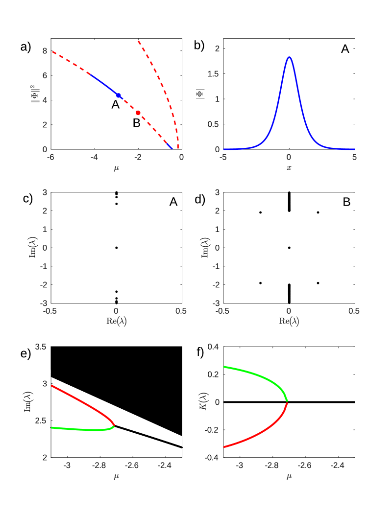
Figure 1: Scarf II potential (4) with $V_{0}=2$, $\gamma=-2.21$. (a) Power curves versus $\mu$. (b) Amplitude profile for point $A$. (c) Spectrum of linearization for point $A$. (d) Same for point $B$. (e) ${\rm Im}(\lambda)$ for the spectrum of linearization versus $\mu$. (f) Krein quantities for isolated eigenvalues versus $\mu$.

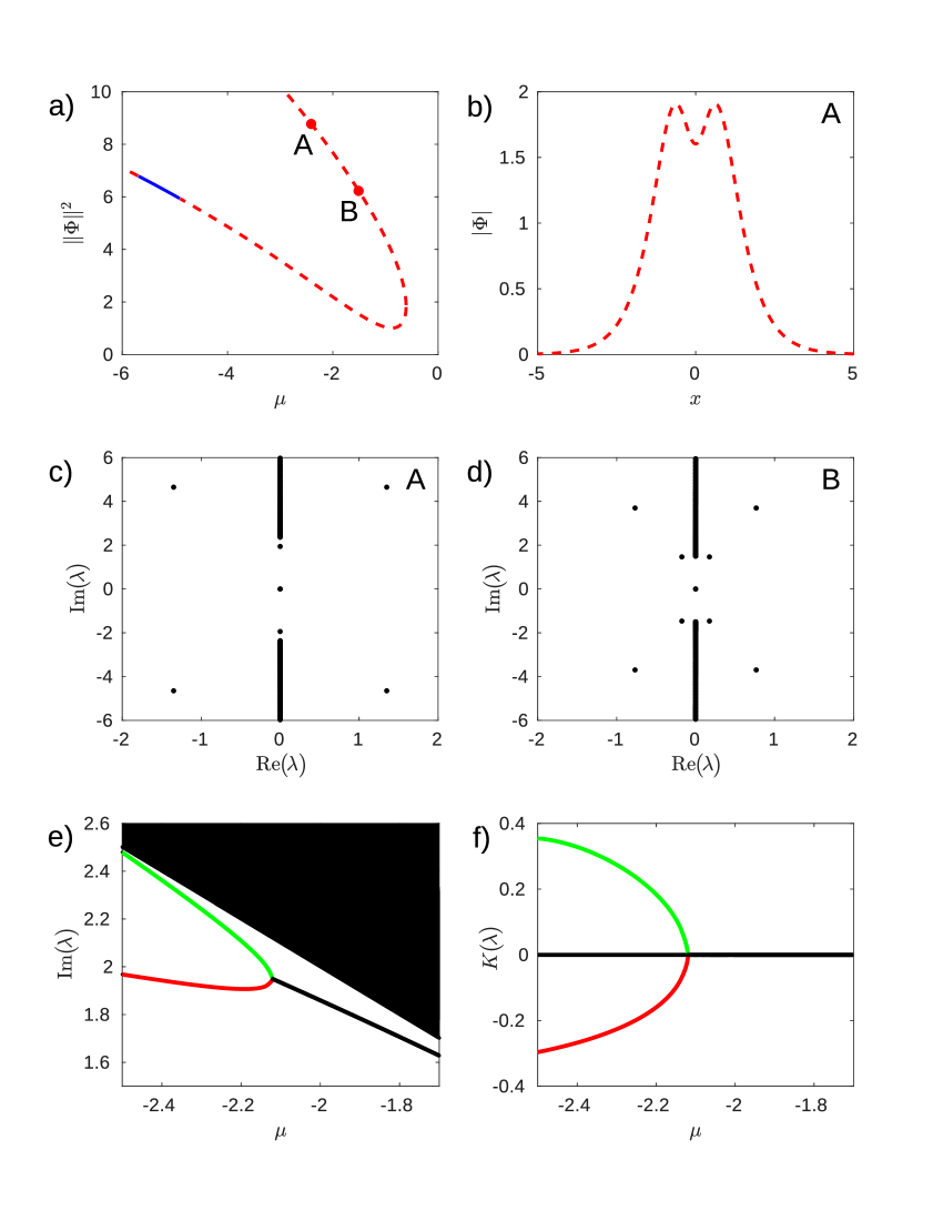
Figure 2: Scarf II potential (4) with $V_{0}=3$, $\gamma=-3.7$. (a) Power curves versus $\mu$. (b) Amplitude profile for point $A$. (c) Spectrum of linearization for point $A$. (d) Same for point $B$. (e) ${\rm Im}(\lambda)$ for the spectrum of linearization versus $\mu$. (f) Krein quantities for isolated eigenvalues versus $\mu$.

Figure 1 (a)-(f) shows the instability bifurcation for the Scarf II potential (4) studied in [27] in the focusing case with $g=1$. Here $V_{0}=2$, $\gamma=-2.21$, and the first branch of the nonlinear modes $\Phi$ is considered. As two eigenvalues with different Krein signatures coalesce, they bifurcate into a complex quadruplet, in agreement with Theorem 1. Note that there’s a small region of stability for the nonlinear modes $\Phi$ of small amplitudes, as it was shown in [27].

Figure 2 (a)-(f) shows the instability bifurcation for the Scarf II potential (4) studied in [6] in the focusing case with $g=1$. Here $V_{0}=3$, $\gamma=-3.7$, and the second branch of the nonlinear modes $\Phi$ is considered. The second branch is unstable with at least one complex quadruplet for all values of parameter $\mu$ used. The imaginary part of this complex quadruplet is not visible on Figure 2 (e) as it coincides with the location of the continuous spectrum. In the presence of this complex quadruplet, we observe a coalescence of two simple eigenvalues $\lambda_{1},\lambda_{2}\in i\mathbb{R}$ and the instability bifurcation into another complex quadruplet. Numerical evidence confirms that the eigenvalues have the opposite Krein signatures prior to collision, allowing us to predict the instability bifurcation, in agreement with Theorem 1.

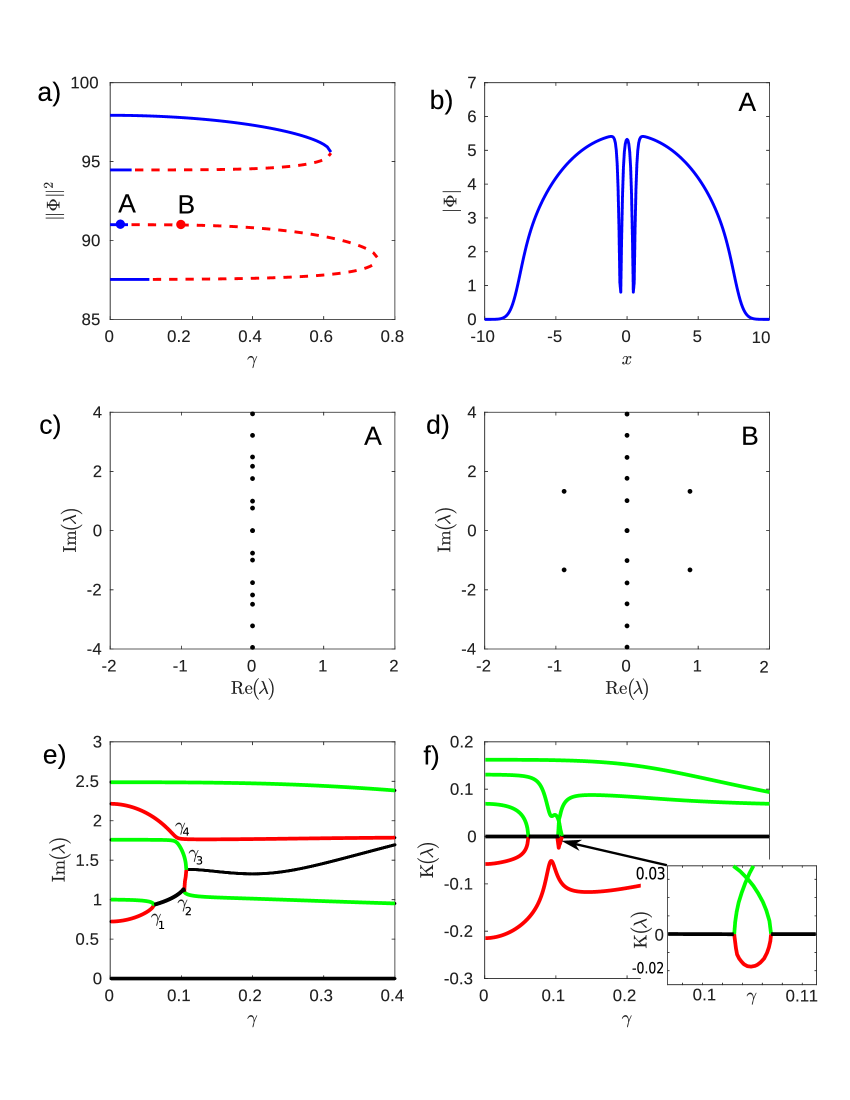
Figure 3: Confining potential (5), scaled as in (46). (a) Power curves versus $\gamma$. (b) Amplitude profile for point $A$. (c) Spectrum of linearization for point $A$. (d) Same for point $B$. (e) ${\rm Im}(\lambda)$ for the spectrum of linearization versus $\gamma$. (f) Krein quantities for isolated eigenvalues versus $\gamma$.

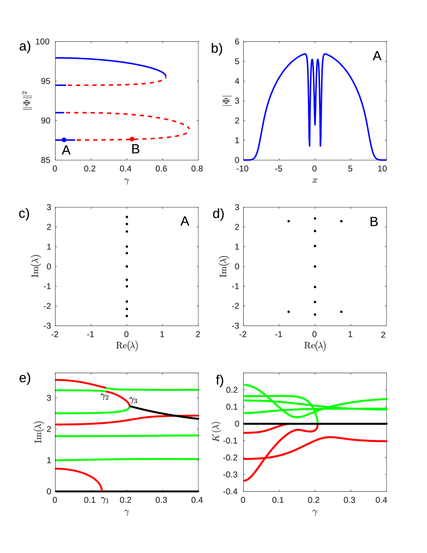
Figure 4: Confining potential (5), scaled as in (46). (a) Power curves versus $\gamma$. (b) Amplitude profile for point $A$. (c) Spectrum of linearization for point $A$. (d) Same for point $B$. (e) ${\rm Im}(\lambda)$ for the spectrum of linearization versus $\gamma$. (f) Krein quantities for isolated eigenvalues versus $\gamma$.

Figures 3,4 (a)-(f) show the confining potential (5) studied in [1], in the defocusing case with $g=-2$. Compared to (5), we use a scaled version of this potential to match the one in [1]:

$$V(x)=x^{2},\quad W(x)=2\Omega^{-3/2}xe^{-\frac{x^{2}}{2\Omega}},$$ (46)

where $\Omega=10^{-1}$ is a scaling parameter. There are four branches of the nonlinear modes $\Phi$ shown, out of which we highlight only the third and fourth branches. The first branch is stable, whereas the second branch becomes unstable because of a coalescence of a pair of eigenvalues $\pm\lambda\in i\mathbb{R}$ with the negative Krein signature at the origin [1]. The third and fourth branches are studied in Figures 3 and 4.

In Figure 3 we can see that there are three bifurcations occurring at $\gamma_{1}\approx 0.07$, $\gamma_{2}\approx 0.1031$ and $\gamma_{3}\approx 0.1069$. For each bifurcation two eigenvalues with different Krein signatures collide and bifurcate off to the complex plane in accordance with Theorem 1. In addition, two simple eigenvalues with different Krein signatures nearly coalesce near $\gamma_{4}\approx 0.1$. Figure 5 (a) shows the norm of the difference between the two eigenvectors and two adjoint eigenvectors for the two simple eigenvalues while $\gamma$ is increased towards $\gamma_{4}$. As the difference does not vanish, we rule out this point as the bifurcation point for the defective eigenvalue. Consequently, the eigenvalues are continued past this point with preservation of their Krein signatures.

In Figure 4 we can see three bifurcations occurring at $\gamma_{1}\approx 0.1303$, $\gamma_{2}\approx 0.1427$, and $\gamma_{3}\approx 0.2078$. At $\gamma_{1}$, an eigenvalue pair with negative Krein signature coalesce at zero and become a pair of real (unstable) eigenvalues. As $\gamma$ is increased towards $\gamma_{2}$, two eigenvalues with opposite Krein signature move towards each other. Figure 5 (b) illustrates that the norm of the difference between the two eigenvectors and the two adjoint eigenvectors vanishes at the coalescence point. Therefore, we conclude that at $\gamma_{2}$ we have a defective eigenvalue which does not split into a complex quadruplet. According to Theorem 1, the defective eigenvalue does not split into complex unstable eigenvalues only if the non-degeneracy condition (30) is not satisfied. Similar safe passing of eigenvalues of opposite Krein signature through each other is observed in [27]. The behavior near $\gamma_{2}$ shows that having opposite Krein signatures prior to coalescence of two simple eigenvalues into a defective eigenvalue is a necessary but not sufficient condition for the instability bifurcation. At $\gamma_{3}$, two eigenvalues with opposite Krein signatures coalesce and bifurcate into a complex quadruplet according to Theorem 1.

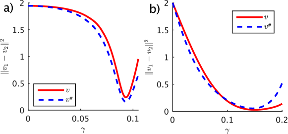
Figure 5: The norm of the difference between the two eigenvectors and the two adjoint eigenvectors prior to a possible coalescence point: (a) for Figure 3 (b) for Figure 4.

6 Discussion

In this work, we introduced the Krein quantity for simple isolated eigenvalues in the linearization of the nonlinear modes in the $\mathcal{PT}$-symmetric NLS equation. We proved that the Krein quantity is zero for complex eigenvalues and nonzero for simple purely imaginary eigenvalues. When two simple eigenvalues coalesce on the imaginary axis in a defective eigenvalue, the Krein quantity vanishes and we proved under the non-degeneracy assumption that this bifurcation point produces complex unstable eigenvalues on one side of the bifurcation point. This result shows that the main feature of the instability bifurcation in Hamiltonian systems is extended to the $\mathcal{PT}$-symmetric NLS equation.

There are nevertheless limitations of this theory in the $\mathcal{PT}$-symmetric systems. First, the adjoint eigenvectors are no longer related to the eigenvectors of the spectral problem, which opens up a problem of normalizing the adjoint eigenvector relative to the eigenvector. We fixed the sign of the adjoint eigenvector in the Hamiltonian limit and continue the sign off the Hamiltonian limit by using continuity of eigenvectors along the parameters of the model.

Second, if the bifurcation point corresponds to a semi-simple eigenvalue, then the bifurcation theory does not lead to the same conclusion as in the Hamiltonian case. The first-order perturbation theory results in the non-Hermitian matrices, hence it is not clear how to conclude on the splitting of the semi-simple eigenvalues on each side of the bifurcation point.

Finally, coalescence of the simple purely imaginary eigenvalues at the origin and the related instability bifurcations are observed frequently in the $\mathcal{PT}$-symmetric systems and they are not predicted from the Krein quantity. Therefore, we conclude that the stability theory of Hamiltonian systems cannot be fully extended to the $\mathcal{PT}$-symmetric NLS equation, only the necessary condition for the instability bifurcation can be, as is shown in this work.

References

- [1] V. Achilleos, P.G. Kevrekidis, D.J. Frantzeskakis, and R. Carretero-González, Dark solitons and vortices in PT-symmetric nonlinear media: From spontaneous symmetry breaking to nonlinear PT phase transitions, Phys. Rev. A 86, 013808 (7 pp) (2012).
- [2] N.V. Alexeeva, I.V. Barashenkov, A.A. Sukhorukov, and Yu.S. Kivshar, Optical solitons in -symmetric nonlinear couplers with gain and loss, Phys. Rev. A 85, 063837 (13 pp) (2012).
- [3] N.V. Alexeeva, I.V. Barashenkov, and Yu.S. Kivshar, Solitons in -symmetric ladders of optical waveguides, New J. Phys. 19, 113032 (30 pp) (2017).
- [4] Z. Ahmed, Real and complex discrete eigenvalues in an exactly solvable one-dimensional complex PT-invariant potential, Phys. Lett. A 282, 343–348 (2001).
- [5] B. Bagchi, R. Roychoudhury, A new PT-symmetric complex Hamiltonian with a real spectrum, J. Phys. A: Math. Gen. 33, L1-L3 (2000).
- [6] I.V. Barashenkov, D.A. Zezyulin, and V.V. Konotop, Exactly solvable Wadati potentials in the PT-symmetric Gross-Pitaevskii equation in Non-Hermitian Hamiltonians in Quantum Physics, Springer Proceedings in Physics 184, 143–155 (Cham, Switzerland, 2016).
- [7] C.M. Bender, Introduction to -symmetric quantum theory, Contemp. Phys. 46, 277–292 (2005).
- [8] C.M. Bender, Making sense of non-Hermitian Hamiltonians, Rep. Prog. Phys. 70, 947–1018 (2007).
- [9] C.M. Bender, B. Berntson, D. Parker, and E. Samuel, Observation of PT phase transition in a simple mechanical system, Am. J. Phys. 81, 173–179 (2013).
- [10] H. Cartarius and G. Wunner, Model of a PT-symmetric Bose-Einstein condensate in a -function double-well potential, Phys. Rev. A 86, 013612 (5 pp) (2012).
- [11] A. Chernyavsky and D.E. Pelinovsky, Breathers in Hamiltonian -symmetric chains of coupled pendula under a resonant periodic force, Symmetry 8, 59 (26 pp) (2016).
- [12] A. Chernyavsky and D.E. Pelinovsky, Long-time stability of breathers in Hamiltonian PT-symmetric lattices, J. Phys. A: Math. Theor. 49, 475201 (20 pp) (2016).
- [13] D. Dast, D. Haag, and H. Cartarius, Eigenvalue structure of a Bose-Einstein condensate in a PT-symmetric double well, J. Phys. A 46, 375301 (19 pp) (2013).
- [14] L. Feng, Z.J. Wong, R. Ma, Y. Wang, and X. Zhang, Single-mode laser by parity-time symmetry breaking, Science 346, 972–975 (2014).
- [15] L. Feng, Y.-L. Xu, W.G. Fegadolli, M.-H. Lu, J.E.B. Oliveira, V.R. Almeida, Y.-F. Chen, and A. Scherer, Experimental demonstration of a unidirectional reflectionless parity-time metamaterial at optical frequencies, Nat. Matter 12, 108–113 (2013).
- [16] B. Heffler, Spectral Theory and its Applications, Cambridge studies in advanced mathematics 139 (Cambridge, New York, 2013).
- [17] H. Hodaei, M.-A. Miri, M. Heinrich, D.N. Christodoulides, and M. Khajavikhan, Parity-time–symmetric microring lasers, Science 346, 975–978 (2014).
- [18] T. Kapitula and K. Promislow, Spectral and dynamical stability of nonlinear waves, Applied Mathematical Sciences 185 (Springer, Berlin, 2013).
- [19] T. Kato, Perturbation theory for linear operators (Springer–Verlag, Berlin, Heidelberg, 1995).
- [20] P.G. Kevrekidis, J. Cuevas–Maraver, A. Saxena, F. Cooper, and A. Khare, Interplay between parity-time symmetry, supersymmetry, and nonlinearity: An analytically tractable case example, Phys. Rev. E 92, 042901 (7 pp) (2015).
- [21] K. Knopp, Theory of functions, part II (Dover, New York, 1947).
- [22] V.V. Konotop, J. Yang, and D.A. Zezyulin, Nonlinear waves in -symmetric systems, Rev. Mod. Phys. 88, 035002 (59 pp) (2016).
- [23] R.S. MacKay, Stability of equilibria of Hamiltonian systems in Nonlinear phenomena and chaos (Malvern, 1985) 254–270, Malvern Physics Series (Hilger, Bristol, 1986).
- [24] K.G. Makris, R. El-Ganainy, D.N. Christodoulides, and Z.H. Musslimani, Beam Dynamics in Symmetric Optical Lattices, Phys. Rev. Lett. 100, 103904 (4 pp) (2008).
- [25] A. Mostafazadeh, Pseudo-Hermitian representation of quantum mechanics, Int. J. Geom. Methods Mod. Phys 07, 1191–1306 (2010).
- [26] Z.H. Musslimani, K.G. Makris, R. El-Ganainy, and D.N. Christodoulides, Optical Solitons in Periodic Potentials, Phys. Rev. Lett. 100, 030402 (4 pp) (2008).
- [27] S. Nixon and J. Yang, Nonlinear wave dynamics near phase transition in PT-symmetric localized potentials, Physica D 331, 48–57 (2016).
- [28] D. Pelinovsky and Y. Shimabukuro, Transverse instability of line solitary waves in massive Dirac equations, J. Nonlin. Sci. 26, 365–403 (2016).
- [29] M. Reed and B. Simon, Methods of modern mathematical physics, Vol. 4: Analysis of Operators (Academic Press, New York, 1978).
- [30] J. Rubinstein, P. Sternberg, and Q. Ma, Bifurcation diagram and pattern formation of phase slip centers in superconducting wires driven with electric currents, Phys. Rev. Lett. 99, 167003 (4 pp) (2007).
- [31] A. Ruschhaupt, F. Delgado, and J.G. Muga, Physical Realization of -symmetric potential scattering in a planar slab waveguide, J. Phys. A: Math Gen. 38, L171–L176 (2005).
- [32] J. Schindler, Z. Lin, J.M. Lee, H. Ramezani, F.M. Ellis, and T. Kottos, -symmetric electronics, J. Phys. A: Math. Theor. 45, 444029 (15 pp) (2012).
- [33] P.D. Hislop and I.M. Sigal, Introduction to Spectral Theory: With Applications to Schrödinger Operators, Applied Mathematical Sciences 113 (Springer, New York, 1995).
- [34] F.L. Scarf, New Soluble Energy Band Problem, Phys. Rev. 112, 1137–1140 (1958).
- [35] M. Stanislavova and A. Stefanov, On the stability of standing waves for symmetric Schrödinger and Klein-Gordon equations in higher space dimensions, Proc. AMS 145, 5273–5285 (2017).
- [36] S.V. Suchkov, A.A. Sukhorukov, J. Huang, S.V. Dmitriev, L. Chaohong, and Yu.S. Kivshar, Nonlinear switching and solitons in PT-symmetric photonic systems, Las. Phot. Rev. 10, 177–213 (2016).
- [37] L.N. Trefethen, Spectral Methods in MATLAB (SIAM, Philadelphia, 2000).
- [38] K. Weierstrass, Mathematische werke, vol. 1 (Johnson Reprint, New York, 1967).
- [39] E. Zeidler, Applied Functional Analysis: Main Principles and Their Applications, Applied Mathematical Sciences 109 (Springer–Verlag, New York, 1995).
- [40] D.A. Zezyulin and V.V. Konotop, Nonlinear modes in the harmonic -symmetric potential, Phys. Rev. A 85, 043840 (6 pp) (2012).