Learning to Schedule Deadline- and Operator-Sensitive Tasks

Abstract

The use of semi-autonomous and autonomous robotic assistants to aid in care of the elderly is expected to ease the burden on human caretakers, with small-stage testing already occurring in a variety of countries. Yet, it is likely that these robots will need to request human assistance via teleoperation when domain expertise is needed for a specific task. As deployment of robotic assistants moves to scale, mapping these requests for human aid to the teleoperators themselves will be a difficult online optimization problem. In this paper, we design a system that allocates requests to a limited number of teleoperators, each with different specialities, in an online fashion. We generalize a recent model of online job scheduling with a worst-case competitive-ratio bound to our setting. Next, we design a scalable machine-learning-based teleoperator-aware task scheduling algorithm and show, experimentally, that it performs well when compared to an omniscient optimal scheduling algorithm.

1 Introduction

Deploying semi-autonomous and autonomous robotic assistants to aid in caring for the elderly is expected to ease the burden on human caretakers. In Japan, for example, the Health, Labor, and Welfare Ministry predicts a shortfall of $380000$ nursing and elderly care workers by $2025$, with similar projected imbalances between supply and demand in other developed nations; thus, this problem is timely Kaneko et al. (2008). Indeed, robotic helpers have already been deployed in small-stage testing in a variety of countries, including Japan, Italy, and Sweden Leiber (2016).

Yet, it is likely that these robots will need to request human assistance—for example, for teleoperation—from time to time. Beyond healthcare, automobile manufacturer Nissan recently announced its plan to augment autonomous vehicle technology with a crew of on-call, remote human “mobility managers” Nowak (2017). As deployment of semi-autonomous robots moves to scale, mapping these requests for human expertise to the teleoperators themselves will be a difficult online optimization problem.

This paper presents a framework for the online allocation of requests to a limited number of specialized teleoperators, each of whom have different levels of expertise for types of requests. We generalize a recent state-of-the-art online scheduling algorithm Lucier et al. (2013) to our setting and test its performance relative to an omniscient offline algorithm. We draw on work in the information retrieval literature to present a novel machine-learning-based method for matching the best job to a specific server at a specific time. We show experimentally that this algorithm performs quite well, beating an adaptation of the closest prior state-of-the-art online scheduling algorithm.

1.1 Related Work

Our problem can be seen as a type of job scheduling, which is a classical problem in computer science and operations research. In our case, the users’ tasks are the jobs and the teleoperators are the machines or servers. We believe our motivation—that of assigning human teleoperators with specific skills to tasks—pushes us to address a novel version of this problem. We briefly overview recent related work at the current research horizon in this space and detail how our work is different; we direct readers interested in a complete history of job scheduling to work by Pinedo Pinedo (2015).

Zheng and Shroff Zheng and Shroff (2016) work in a setting where jobs arrive online, and give some partial value for partial execution. Doucette et al. Doucette et al. (2016) address assigning jobs to agents in an online fashion, and also with preemption of previously allocated jobs in a distributed setting. Neither address jobs’ preference for specific servers (as we will, where a job completed on a preferred servers yields greater utility), nor servers’ heterogeneous completion rate for a job type. Most related to our work, Lucier et al. Lucier et al. (2013) look at online allocation of batch jobs with deadlines to identical servers; we generalize their model to a setting with heterogeneous servers and where the jobs have preferences over servers.

From a learning theory point of view, some recent work takes a regret-minimization approach to online job scheduling Even-Dar et al. (2009); however, that work is motivated by allocating users/connections to different links via a load balancer and assumes that no knowledge of the job’s runtime is known ahead of time (as in our case). Rather, the job’s runtime is known once it is assigned to a handler. From an applied machine learning point of view, job scheduling with a classification component has recently gained attention Tripathy et al. (2015); Panda et al. (2015); most of this work focuses on offline scheduling of jobs with dependencies and deadlines, while we focus on online scheduling of independent jobs. Gombolay et al. Gombolay et al. (2016) take a reinforcement learning approach to the apprenticeship problem, that is, learning human-quality heuristics; they do this by way of a pairwise ranking function, as we do, but their setting is not online.

From the operations management point of view, Pérez et al. Pérez et al. (2013) focus on the nuclear medicine application area, and take a two-stage stochastic IP approach to scheduling patients that arrive with multi-step tests, e.g., a patient arrives with three tests that have to be performed sequentially, but an individual job cannot be paused once it has started. In their model, once a patient’s jobs are scheduled (in the future), they cannot be changed, a constraint we do not have. Anderson Anderson (2014) provides state-of-the-art techniques for scheduling residents in hospitals under various constraints; we direct the reader to his work for an in-depth survey of such approaches. We note that our proposed model would be useful in a setting such as scheduling residents to hospitals, and can be seen as addressing a version of that problem.

1.2 Our Contributions

This paper presents a machine-learning-based approach to a novel generalization of a classical problem in computer science and operations research. Motivated by the increasing presence of semi-autonomous robots that need to “call out” to human teleoperators, we address the online job scheduling problem where jobs have preferences over which server (teleoperator) completes them, and teleoperators have varying skill levels for completing specific classes of jobs. We extend a recent model of online job scheduling to this setting, give a competitive ratio for a simple generalization of an algorithm in that space, and then present a sophisticated machine-learning-based approach to scheduling jobs. We draw on intuition from the information retrieval literature to learn a ranking function of jobs for servers. We validate our approach in simulaton and show that it outperforms a generalization of the state-of-the-art algorithm for our setting.

2 A Model for Scheduling Jobs with Preferences to Heterogeneous Servers

In this section, we formalize our model. It generalizes a recent model due to Lucier et al. Lucier et al. (2013).

2.1 Our Model

Lucier et al. Lucier et al. (2013) work in a setting where jobs $j\in\mathcal{J}{}$ arrive online at time $a_{j}$ with a deadline $d_{j}$ indicating the last time period at which a job can be completed, and a processing time $p_{j}$ indicating a base level of resource consumption. Upon completion, jobs yield a value $v_{j}$. Their model assumes all servers are identical; we will change this later.

They provide an online algorithm for this setting that aims to maximize the total value of completed jobs, and prove a lower bound (worst-case competitive ratio) on the performance of the proposed online scheduling algorithm, by ordering the jobs according to their value-density–for a job $j$, defined to be $\rho_{j}=\frac{v_{j}}{p_{j}}$, the ratio of value to processing time. They allow scheduling to occur only when a new job arrives or when a job completes execution. Additionally, server-affinity is assumed; that is, when a task is scheduled to a specific server it will not “migrate” to another server, even when the job is preempted and other servers are idle.

Their scheduling algorithm also relies on three concepts, which we will also use in our generalization of that model. For a given job $j\in\mathcal{J}{}$, let the $s_{j}=\frac{d_{j}-a_{j}}{p_{j}}$ be the minimum slack necessary for a task to be accepted, which is the ratio of the available time for the task to its processing time. This is compared against a global slack parameter $s$, a hyper-parameter to any scheduling algorithm.

Similarly, let $W^{-\mu}_{j}$ be the time interval $\{a_{j},\ldots,d_{j}-\mu p_{j}\}$ and $A^{-\mu}(t)=\{j\in\mathcal{J}{}\ |\ t\in W^{-\mu}\}$ the set of jobs at time $t$ with a remaining execution window of $\mu$ times the processing time $p_{j}$. Finally, define a preemption threshold $\gamma$; a job $j_{2}$ will preempt another job $j_{1}$ only if the ratio of their value-densities is greater than $\gamma$, i.e., $\rho_{j_{2}}>\gamma\rho_{j_{1}}$.

The principles of attaining value only from fully completed jobs and continuing execution on a single server fit well with the requirements of our use cases, including teleoperators assisting elderly patients, or humans assisting semi-autonomous vehicles. However, we note that in our setting, not all servers (teleoperators) are equally skilled. That is, a registered nurse may be quite skilled at helping a geriatric human perform a life task, but less skilled at teleoperating a car through a snowstorm. Furthermore, it may be the case that a geriatric human would get greater value from interacting with the registered nurse than with the incliment-weather-trained driver. Thus, we extend the model of Lucier et al. Lucier et al. (2013) with the notion of non-identical servers and job preferences, by adding the following attributes:

1. We categorize jobs into discrete types $\tau$.

2. Each server $i$ has a scalar efficiency $\eta^{i}_{\tau}\in(0,1]$ for each job type $\tau$. The efficiency accounts for the varying proficiency of the servers for the different types of jobs, and modifies the actual execution time of a job of type $\tau$ according to its original processing time, such that $p_{j}^{\prime}=\frac{p_{j}}{\eta^{i}_{\tau}}$.

3. Each job $j$ expresses a scalar preference for each server $i$, defined as $\psi^{i}_{j}\in(0,1]$. This preference modifies the value gained by completion of the job, $v_{j}^{\prime}=\psi^{i}_{j}v_{j}$.

Symbol	Description
$a_{j}$	arrival time
$d_{j}$	job completion deadline
$p_{j}$	nominal processing time
$v_{j}$	value received upon job completion
$\rho_{j}$	value-density, ratio of $v_{j}$ to $p_{j}$
$s_{j}$	slack of a job
$s$	global slack parameter
$W^{-\mu}_{j}$	time interval $[a_{j},d_{j}-\mu p_{j}]$
$A^{-\mu}(t)$	the set of jobs $j$ at time $t$ with availability at least $\mu$ times $p_{j}$
$\gamma$	preemption threshold between jobs
$\tau_{j}$	job type
$\eta^{i}_{\tau}$	efficiency of server $i$ for job type $\tau$
$\psi^{i}_{j}$	preference of job $j$ for a server $i$

Table 1: Notation.

Table 1 summarizes the notation that we use from Lucier et al. Lucier et al. (2013), as well as the notation we introduced to create our new model.

2.2 A Simple Scheduling Algorithm

Given this generalized model, how should we allocate arriving jobs to servers? Similarly, if a job completes on a server, which queued job should be allocated to that newly-idle server? In Section 3, we present a sophisticated machine-learning-based approach to answer these questions; however, first, we generalize a recent state-of-the-art scheduling algorithm, again due to Lucier et al. Lucier et al. (2013), to our model.

First, for any job $j$ and server $i$, define the server-dependent value-density $\dot{\rho}^{i}_{j}=\rho_{j}\psi^{i}_{j}\eta^{i}_{\tau}$, where $\tau$ is the type of job $j$. This is a straightforward adaptation of the value-density metric to the case of heterogeneous servers (via the $\eta^{i}_{\tau}$ multiplier) and job preference over servers (via the $\psi^{i}_{j}$ multiplier). We then adapt the scheduling algorithm of Lucier et al. Lucier et al. (2013) to account for the varying nature of the servers by using the server-dependent value-density, and by comparing that value-density difference between the value-density of a candidate job on a specific server and the value-density of running job on that server (zero for idle servers) when making a preemption decision. That algorithm, for multiple servers, is given below as Algorithm 1.

Event Type 1: A job $j$ arrived at time $t=a_{j}$.

1. calculate delta value-density ($\rho$) for servers:

   $\forall i\in\mathit{servers},\Delta\rho^{j}_{i}=\rho^{j}_{i}-\rho_{i}$

2. choose server with highest change to value-density

   $i=\underset{i}{\operatorname{arg}\,\operatorname{max}}\;\Delta\rho^{j}_{i}$

3. call the threshold preemption rule (i,t)

Event Type 2: A job $j$ completes on server $i$ at time $t$.

1. Resume execution of the preempted job $j$ with highest server-dependent value-density $\dot{\rho}^{i}_{j}$ among any job preempted on $i$

2. Call the threshold preemption rule below with server $i$ and time $t$

Threshold Preemption Rule ($i$, $t$):

1. Let $j$ be the job currently being processed on server $i$

2. Let $j^{*}=\underset{j}{\operatorname{arg}\,\operatorname{max}}\;\{\dot{\rho}^{i}_{j^{*}}\ |\ j^{*}\in A^{-\mu}(t)\}$

3. If $(\dot{\rho}^{i}_{j^{*}}>\gamma\dot{\rho}^{i}_{j})$: preempt $j$ in favor of $j^{*}$ on server $i$

Algorithm 1 Adapted Online Job Scheduling Algorithm

In practice, the performance of Algorithm 1—which we call the value-density algorithm for scheduling, or VDaS—can be tuned according to the specific distribution incoming jobs by conducting a grid search on the hyperparameters such as $\mu$, $\gamma$, and the slack $s$. We do just this in our experimental Section 4, to ensure the algorithm’s competitiveness given our simulation’s parameterization. Next, in Section 3, we design a machine-learning-based approach to solving our online scheduling algorithm and show that, in practice, it outperforms the algorithm above.

3 Learning to Schedule

In this section, we describe a method that learns to place jobs on servers, based on features of both the incoming job and idle servers, but also more global features like the state of all assignments and historical preemption. Indeed, we try to learn an optimal scheduling function, defined against an (unattainable) gold standard omniscient offline scheduling algorithm, as described in Section 3.1. We use that algorithm to generate training data to fit a comparator network Rigutini et al. (2011) that ranks placement decisions, described in Section 3.2. Building on this, Section 3.3 gives Ranking, our learning-based online scheduling algorithm.

3.1 Gold Standard: Optimal Scheduling Function

Our goal is to use machine learning methods to learn a good scheduling function—in this case, one that is as close as possible to an optimal offline scheduling algorithm. We start by solving the optimal offline scheduling problem on small-sized scenarios and recording the scheduling decisions; we use this as target labels for our training data during a supervised learning phase discussed in the following section.

Although the optimal offline scheduling is known to be NP-hard Pinedo (2015), we scaled the problem so that it could be solved within reasonable time with a MIP solver Gurobi Optimization (2016), using $40$ jobs of $3$ types scheduled to $4$ servers with tight timing constraints (to reduce the number of decision variables). We solved over a thousand such scenarios, under constraints that ensure feasibility:

1. capacity: only one task is executed at a time on each of the servers;

2. affinity: a task can only be executed on a single server;

3. demand: a task can either be completely scheduled to satisfy its processing demand or not scheduled at all;

4. scheduling window: a task can only be executed between its arrival and deadline; and

5. event based scheduling: scheduling and preemption can only occur when a new task arrives or completes.

In order to minimize unnecessary affinity constraints, arriving jobs which are not scheduled are kept in an “unassigned pool” which can be scheduled to any of the servers.

3.2 Learning to Rank & Learning to Schedule

We now draw on intuition from the information retrieval literature to learn a ranking function that will be incorporated into a scheduling algorithm which is described in Section 3.3,.

We note that scheduling decisions involve choosing the “best” job for a specific server, and choosing the “best” server for a specific job. Complications in this space include deciding on which features to use, how to quantify the quality of a specific job-server match, and that the number of jobs and servers involved in each scheduling decision is different—thus, it is difficult to train a function with variable-sized input.

Yet, this sort of task is common in information retrieval, where documents need to be ranked according to their match to a given query. Ranking documents shares the complexities enumerated above, including the presence of a variable number of documents per query as well as unknown ranking function.

With this in mind, we apply the cmpNN architecture Rigutini et al. (2011) to our domain, and use it to learn a pairwise comparison function of two scheduling options.

The cmpNN architecture is an artificial neural network based on two shared layers which are connected anti-symmetrically. The input to the network consists of two vectors of equal size, and the output consists of two neurons which stand for $[x\succ y,y\succ x]$. This architecture has the following properties:

1. reflexivity: for identical input vectors, the network produces identical output (regardless of input ordering); and

2. equivalence: if $x\succ y$ then $y\prec x$ and vice versa. More precisely, swapping the input vectors results in swapping of the output neurons: $[o_{1},o_{2}]=f(\vec{x},\vec{y})\iff[o_{2},o_{1}]=f(\vec{y},\vec{x})$.

The only attribute missing to make this network an ideal comparator is transitivity, i.e. ensuring that if $x\succ y$ and $y\succ z$ then $x\succ z$, but as we will demonstrate this shortcoming does not limit the network’s ranking ability in real world scenarios.

The Network. We extended the architecture in two ways.

1. Deeper network: the original network used a single hidden layer, which did not train well on our data. Our network uses three hidden layers of decreasing width, while maintaining the shared layer architecture at each hidden layer. The dimension of the first hidden layer is derived from the dimension of the input vectors: $h_{1,\mathit{dim}}=2^{\lceil\lg(x_{\mathit{dim}})\rceil+6}$, with successive layers “shrinking” by a factor of two. The activation of the first two hidden layers is $\tanh$ and the third and fourth layers have a ReLU activation.

2. Probabilistic output: the two output neurons of the original architecture are connected to a softmax activation, this provides a probabilistic measure for the comparison, i.e. what is the probability that $x\succ y$. Moreover, this enables using the categorical-crossentropy loss function which improves the learning convergence

The network architecture is shown in Figure 1. The symmetric nature of the network is built by sharing weights as can be demonstrated for the connection between the input and the first hidden layer:

$$\vec{w}_{i,1}^{\,1} =w(\vec{X}\to H_{1,1})=w(\vec{Y}\to H_{1,2})$$

$$\vec{w}_{i,1}^{\,2} =w(\vec{X}\to H_{1,2})=w(\vec{Y}\to H_{1,1}).$$

The bias term of both parts of the first hidden layer is also shared. Thus, the two output vectors of the first hidden layer are:

$$\vec{v}_{1,1} =\tanh(\vec{w}_{i,1}^{\,1}\cdot\vec{X}+\vec{w}_{i,1}^{\,2}\cdot\vec{Y}+\vec{b}_{1})$$

$$\vec{v}_{1,2} =\tanh(\vec{w}_{i,1}^{\,1}\cdot\vec{Y}+\vec{w}_{i,1}^{\,2}\cdot\vec{X}+\vec{b}_{1})$$

The rest of the layers share weights and connections in a similar fashion with their appropriate activation functions.

Figure 1: Pairwise comparator scheduling network.

The Features. We used a set of features that combine a description of the candidate job as well as that of the server; this way, a single comparator network can be used to compare jobs for a given server, and to compare servers for a given job. (Due to space, we omit the list of features.)

The combined job/server feature vector enables to perform the two type of comparisons we initially desired:

1. ranking two servers ($i_{1}$, $i_{2}$) for a given job ($j$): $\text{rank}([j,i_{1}],[j,i_{2}])$; and

2. ranking two jobs ($j_{1}$, $j_{2}$) for a given server ($i$): $\text{rank}([j_{1},i],[j_{2},i])$.

Training samples can be taken by analyzing the optimal scheduler decision for each of the two types of scheduling events:

1. On arrival of a new job $j_{a}$:

   • If the job $j_{a}$ gets scheduled:

     1. Compare new job $j_{a}$ with all other jobs—preempted $\mathcal{P}^{i}$ or unassigned $\mathcal{U}$—on the selected server $i$, requiring $\forall j_{k}\in{\mathcal{P}^{i}\cup\mathcal{U}},[j_{a},i]\succ[j_{k},i]$

     2. Compare new job $j_{a}$ with selected server $i$, versus other servers $k\neq i,[j_{a},i]\succ[j_{a},k]$

   • If the job $j_{a}$ does not get scheduled:

     1. Compare new job $j_{a}$ against all running jobs,
        $\forall i\in\text{active-servers},[j_{a},i]\prec[j_{i},i]$

2. On the completion of a job:

   • If another job $j$ is scheduled:

     1. Compare job $j$ against other pending and unassigned jobs

     2. If job $j$ was from the unassigned pool, compare that job against other servers

3.3 The Ranking Algorithm

We now present our online job scheduling algorithm that incorporates the comparator network discussed above. We build on Algorithm 1 (without its hyperparameters). The adaptation is given below as Algorithm 2.

Event Type 1: Jobs {$j_{k}$} arrive at time $t=a_{j}$.

while available servers for unscheduled job $\in\{j_{k}\}$ do

1. Calculate top-ranking server for each job;

2. Resolve multiple assignments to same server according to server’s ranking of the jobs;

3. Schedule job/server pairs;

Event Type 2: Servers $\{i_{k}\}$ completes its job at time $t$.

while available jobs for idle server $\in{i_{k}}$ do

1. Calculate top-ranking job (among those preempted in this server that are unassigned) for each server;

2. Resolve multiple assignments to the same job according to that job’s ranking of the servers; and

3. Schedule job/server pairs.

Algorithm 2 The Ranking scheduling algorithm.

At a high level, Algorithm 2 performs as follows. When a job is completed, a pairwise comparison is performed on all jobs which are unassigned or were preempted on this server. The pairwise comparison is akin to the first pass of bubble sort, yielding the top ranking job at the top of the list. Since multiple jobs can be completed at the same time step, we need to accommodate for conflicts, i.e., two servers selecting the same unassigned job. Thus, all potential scheduling assignments are saved during this step, and for each conflict (two or more servers selecting a job), we let the job break the tie by comparing two vectors of the same job with the conflicting servers, and the job is removed from the unassigned pool. Servers which “lost” the contentious job, return to the first phase to select another job. The process continues until no more possible matches are available.

Similarly, when a job arrives, it initially builds a list of all candidate servers, composed of the idle servers, and servers whose running job “loses” to the new job ($[j_{a},i]\succ[\mathit{run}_{i},i]$). As above, multiple jobs can arrive at the same time step, and can request the same server. The conflicts are resolved, this time, from the other side; servers “decide” by comparing the combination of the server with conflicting jobs. This time, jobs which “lost” their requested server return to the first phase of the arrival event.

Next, we compare Algorithm 1 (VDaS) and Algorithm 2 (Ranking) against the offline optimal solution, when available, and against each other on larger simulated instances.

4 Experimental Validation

In this section, we compare the performance of the online scheduling VDaS and Ranking algorithms presented in Sections 2 and 3, respectively. To ensure a fair comparison, we performed a standard model selection grid search over the hyperparameters $\mu$ and $\gamma$ for Algorithm 1 (VDaS); we trained the competing Ranking algorithm’s comparator network only on “small” scenarios, to be described later. We find that Ranking attains much greater value from completed jobs in the case where servers are homogeneous (§4.1), as well as when the servers are heterogeneously specialized (§4.2), for varying levels of heterogeneity.

4.1 Online Scheduling Performance

We begin by comparing both algorithms in a simulation involving jobs arriving in an online fashion to a set of servers. The evaluation metric is the total value attained from completed jobs of random scenarios. In our simulation, a job $j$ arrives randomly with processing demand drawn uniformly at random $p_{j}\in[5,31]$, slack $s_{j}\in[1.5,4.0]$, value $v_{j}\in[50,200]$, and one of three random types $\tau$. The preference of that job $j$ for each server $i$ is drawn uniformly at random as $\psi_{j}^{i}\in[0.5,1]$. Servers $i$ are initialized with a random efficiency value $\eta^{i}_{\tau}\in[0.5,1]$ at the beginning of the simulation for each type $\tau$.

We perform a standard model selection technique for VDaS—a grid search over the relevant hyperparameters $\mu$ and $\gamma$. We also train the comparator network of Ranking only on our smallest simulation, that is, $40$ jobs and $4$ servers. As we will see, this network generalizes quite well, and the performance of Ranking remains high—much higher than VDaS—during larger simulations.

For smaller simulations, we compare both algorithms’ performance against a prescient offline optimal schedule that maximizes value, which is computed by solving a mixed integer linear program (MILP) using the Gurobi optimization toolkit Gurobi Optimization (2016). For larger simulations, this optimal solution is intractable to compute, so we compare the two algorithms only to each other.

We begin with a small simulation: $40$ jobs arriving to $4$ servers. Figure 2(a) compares both algorithms to the optimal offline solution (value $1.0$); while neither algorithm achieves the omniscient optimum, both perform well. Yet, the mean fraction of optimal achieved by Ranking is over $5\%$ higher than VDaS. Figure 2(b) provides an alternative view; here, we take each of the over $1000$ runs, sort them by the fraction of optimal achieved by VDaS, and then plot the performance of Ranking on the same seed. While there are times when VDaS outperforms Ranking, the latter algorithm outperforms the former the majority of the time.

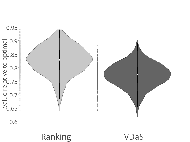
(a) Relative comparison against an offline omniscient schedule.

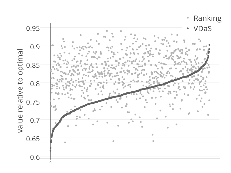
(b) Comparison of VDaS and Ranking on identical runs.

Figure 2: Small test case: $40$ jobs and $4$ servers

When scaling up the scenario size, we no longer have the offline optimal value—solving the offline optimal MILP quickly becomes intractable. The following experiments directly compare the two algorithms, with $1.0$ now representing the highest value achieved by one of the two algorithms.

We now test with $1000$ jobs arriving to $100$ servers. Figure 3(a) corresponds to Figure 2(a), showing the distribution of values achieved by both algorithms. The two algorithms’ performances are nearly separated at this point, with Ranking dramatically outperforming VDaS—even thought its internal comparator network was trained on a dramatically simpler scenario. Figure 3(b) corresponds to Figure 2(b); however, on these larger simulations, Ranking always achieves greater aggregate value than VDaS.

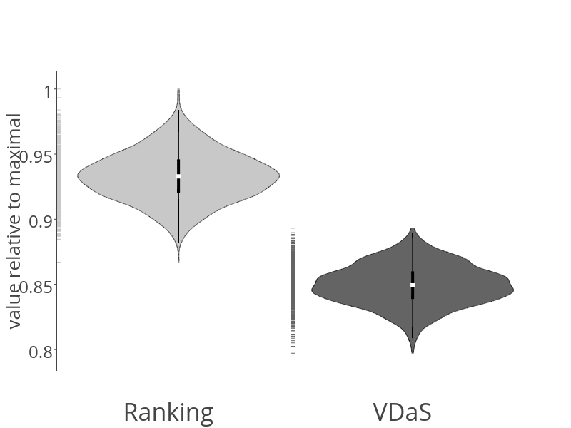
(a) Comparison of VDaS and Ranking.

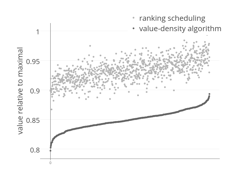
(b) Comparison of VDaS and Ranking on identical runs.

Figure 3: Large test case: $1000$ jobs and $100$ servers

A performance gap between the algorithms that grows with the size of the simulation can be explained as follows. As the number of servers increases, the probability of randomly selecting the “correct” server decreases with the number of available servers. The probability of multiple jobs arriving together (or completing together) grows with the number of jobs. The server-affinity constraint (which both algorithms obey), in our setting of non-identical servers, incurs a performance penalty for “incorrect” assignments. This was not the case in the homogeneous server work of Lucier et al. Lucier et al. (2013).

4.2 Varying the Expertise of the Servers

Recalling our motivation—specialized human teleoperators providing assistance to the needy—we now test the effect of increased server specialization on algorithm performance in the following two settings:

1. A small group of highly-trained servers with high efficiency, versus a larger group of servers with lower efficiency ($\eta$) over types, where the ratio of the efficiency was tuned to match the change in the number of server, thus, in theory, allowing for similar throughput. In this setting, we fix the preferences that each job $j$ has over a server $i$ $\psi^{i}_{j}$; this was done to decrease variance and increase the focus on the server’s varying efficiency.

2. Two groups of the same number of servers. One group has average efficiency over all job types, while the other group has $1/\#\text{types}$ servers with high efficiency for a single type. We normalize the efficiency parameters to achieve similar throughput and the preference factor that a job has for a server is kept fixed, as motivated above.

Figure 4 demonstrates the first test case, where $4$ groups of servers have efficiencies $\eta\in\{0.60,0.75,0.82,0.90\}$, with a lower number of servers in the groups with higher efficiency. We see that in each setting, Ranking outperforms VDaS, and that the performance grows with the efficiency of the servers only in the Ranking algorithm. Again, this is likely due to the high cost of selecting the “wrong” server.

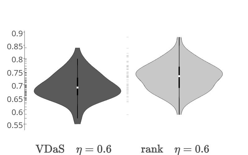
(a) $\eta=0.60$

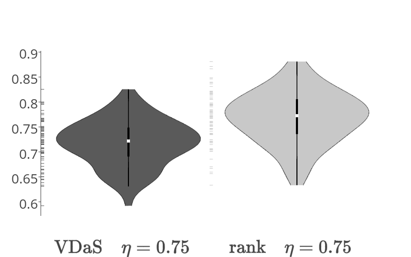
(b) $\eta=0.75$

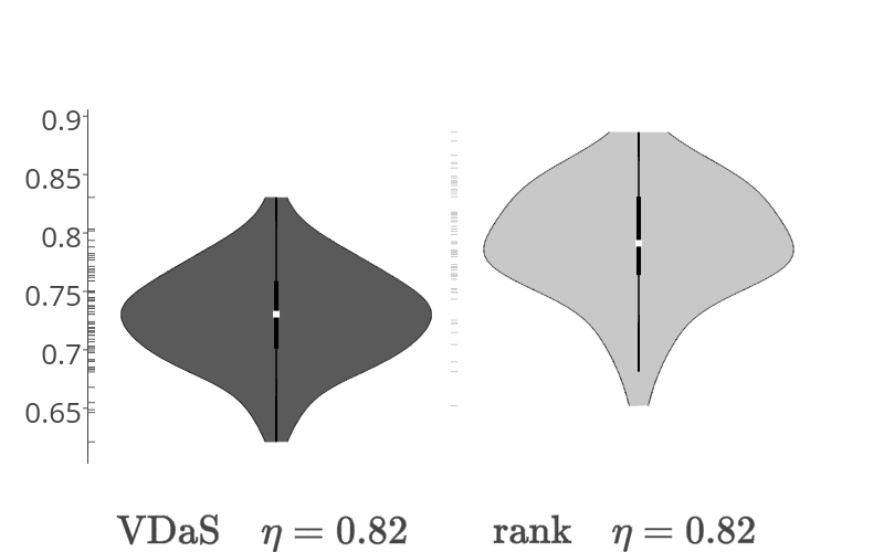
(c) $\eta=0.82$

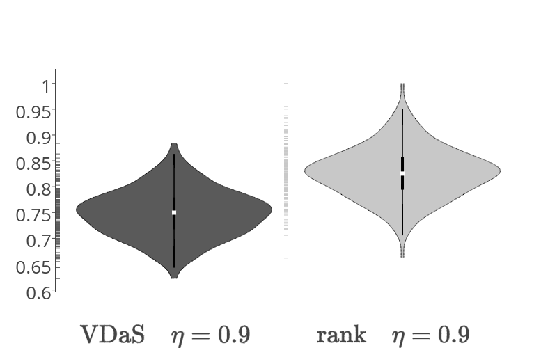
(d) $\eta=0.90$

Figure 4: Comparing the performance of VDaS and Ranking as the efficiency of servers $\eta$ increases.

We now move to the second test case, where two equally-sized groups have either average but broad efficiency, or high but specialized efficiency. Figure 5 compares the performance of VDaS and Ranking on the group with average but uniform efficiency, the second group of specialized servers. Figure 5(a) compares both algorithms when the efficiency of the “average” group is $\eta=0.7$, and the “specialized” group is with efficiencies in $\{0.63,0.63,0.9\}$. Figure 5(b) provides a similar analysis on parameters with lower variance: $\eta=0.8$ for the average group, and $\{0.76,0.76,0.9\}$ for the specialized group. We see that Ranking outperforms VDaS in all the scenarios. Furthermore, and as a testament to the comparator network, Ranking achieves more values as specialization increases, while VDaS does not.

(a) high variance

(b) low variance

Figure 5: Comparing the performance of VDaS and Ranking as specialization heterogeneity increases.

5 Conclusions & Future Research

Motivated by the increasing presence of semi-autonomous robots that “call out” to human teleoperators, this paper presented a machine-learning-based approach to the online job scheduling problem where jobs (tasks) have preferences over which server (teleoperator) completes them, and teleoperators have varying skill levels at completing specific classes of tasks. We extended a recent model of online scheduling to this setting, and then presented an approach to scheduling tasks that learns a ranking function of jobs for servers. We validated our approach in a simulation; it outperformed a generalization of the state-of-the-art algorithm for our setting.

Future research could consider fairness metrics like “no starvation” and proportional care; this is of independent theoretical and practical interest. Considering more elaborate tiebreaking rules—for example, by drawing intuition from the Hungarian algorithm or stable matching—when a job conflicts with two or more servers might complement fairness or increase overall efficiency. The moral and ethical issues that arise when using autonomous or semi-autonomous help for care or driving Stock et al. (2016), or AI systems that make decisions autonomously Conitzer et al. (2017), must be considered.

References

- Anderson [2014] Ross Anderson. Stochastic models and data driven simulations for healthcare operations. PhD thesis, Massachusetts Institute of Technology, 2014.
- Conitzer et al. [2017] Vincent Conitzer, Walter Sinnott-Armstrong, Jana Schaich Borg, Yuan Deng, and Max Kramer. Moral decision making frameworks for artificial intelligence. In AAAI Conference on Artificial Intelligence (AAAI), 2017.
- Doucette et al. [2016] John A Doucette, Graham Pinhey, and Robin Cohen. Multiagent resource allocation for dynamic task arrivals with preemption. ACM Transactions on Intelligent Systems and Technology (TIST), 8(1):3, 2016.
- Even-Dar et al. [2009] Eyal Even-Dar, Robert Kleinberg, Shie Mannor, and Yishay Mansour. Online learning for global cost functions. In Conference on Learning Theory (COLT), 2009.
- Gombolay et al. [2016] Matthew Gombolay, Reed Jensen, Jessica Stigile, Sung-Hyun Son, and Julie Shah. Apprenticeship scheduling: Learning to schedule from human experts. In Proceedings of the International Joint Conference on Artificial Intelligence (IJCAI), 2016.
- Gurobi Optimization [2016] Inc. Gurobi Optimization. Gurobi optimizer reference manual, 2016.
- Kaneko et al. [2008] Ryuichi Kaneko, Akira Ishikawa, Futoshi Ishii, Tsukasa Sasai, Miho Iwasawa, Fusami Mita, and Rie Moriizumi. Population projections for japan: 2006-2055 outline of results, methods, and assumptions. The Japanese Journal of Population, 6(1), 2008.
- Leiber [2016] Nick Leiber. Europe bets on robots to help care for seniors. Bloomberg BusinessWeek, March 2016. Accessed: 2016-08-23.
- Lucier et al. [2013] Brendan Lucier, Ishai Menache, Joseph Seffi Naor, and Jonathan Yaniv. Efficient online scheduling for deadline-sensitive jobs. In ACM Symposium on Parallelism in Algorithms and Architectures (SPAA), pages 305–314. ACM, 2013.
- Nowak [2017] Peter Nowak. Nissan uses NASA rover tech to remotely oversee autonomous car: New Scientist, 2017. [Online; accessed 2017-02-12].
- Panda et al. [2015] Sunita Panda, Pradyumna K. Mohapatra, and Siba Prasada Panigrahi. A new training scheme for neural networks and application in non-linear channel equalization. Applied Soft Computing, 27:47 – 52, 2015.
- Pérez et al. [2013] Eduardo Pérez, Lewis Ntaimo, César O Malavé, Carla Bailey, and Peter McCormack. Stochastic online appointment scheduling of multi-step sequential procedures in nuclear medicine. Health Care Management Science, 16(4):281–299, 2013.
- Pinedo [2015] Michael Pinedo. Scheduling. Springer, 2015.
- Rigutini et al. [2011] Leonardo Rigutini, Tiziano Papini, Marco Maggini, and Franco Scarselli. SortNet: Learning to rank by a neural preference function. IEEE Transactions on Neural Networks, 22:1368–1380, 2011.
- Stock et al. [2016] Oliviero Stock, Marco Guerini, and Fabio Pianesi. Ethical dilemmas for adaptive persuasion systems. In AAAI Conference on Artificial Intelligence (AAAI), 2016.
- Tripathy et al. [2015] Binodini Tripathy, Smita Dash, and Sasmita Kumari Padhy. Dynamic task scheduling using a directed neural network. Journal of Parallel and Distributed Computing, 75:101 – 106, 2015.
- Zheng and Shroff [2016] Zizhan Zheng and Ness B Shroff. Online multi-resource allocation for deadline sensitive jobs with partial values in the cloud. In IEEE International Conference on Computer Communications (INFOCOM), 2016.