Rigorous Dynamics and Consistent Estimation in Arbitrarily Conditioned Linear Systems

Abstract

The problem of estimating a random vector $\mathbf{x}$ from noisy linear measurements $\mathbf{y}=\mathbf{A}\mathbf{x}+\mathbf{w}$ with unknown parameters on the distributions of $\mathbf{x}$ and $\mathbf{w}$, which must also be learned, arises in a wide range of statistical learning and linear inverse problems. We show that a computationally simple iterative message-passing algorithm can provably obtain asymptotically consistent estimates in a certain high-dimensional large-system limit (LSL) under very general parameterizations. Previous message passing techniques have required i.i.d. sub-Gaussian $\mathbf{A}$ matrices and often fail when the matrix is ill-conditioned. The proposed algorithm, called adaptive vector approximate message passing (Adaptive VAMP) with auto-tuning, applies to all right-rotationally random $\mathbf{A}$. Importantly, this class includes matrices with arbitrarily bad conditioning. We show that the parameter estimates and mean squared error (MSE) of $\mathbf{x}$ in each iteration converge to deterministic limits that can be precisely predicted by a simple set of state evolution (SE) equations. In addition, a simple testable condition is provided in which the MSE matches the Bayes-optimal value predicted by the replica method. The paper thus provides a computationally simple method with provable guarantees of optimality and consistency over a large class of linear inverse problems.

I Introduction

Consider the problem of estimating a random vector $\mathbf{x}^{0}$ from linear measurements $\mathbf{y}$ of the form

$$\mathbf{y}=\mathbf{A}\mathbf{x}^{0}+\mathbf{w},\quad\mathbf{w}\sim{\mathcal{N}}(\mathbf{0},\theta_{2}^{-1}\mathbf{I}),\quad\mathbf{x}^{0}\sim p(\mathbf{x}|{\bm{\theta}}_{1}),$$ (1)

where $\mathbf{A}\in{\mathbb{R}}^{M\times N}$ is a known matrix, $p(\mathbf{x}|{\bm{\theta}}_{1})$ is a density on $\mathbf{x}^{0}$ with parameters ${\bm{\theta}}_{1}$, $\mathbf{w}$ is additive white Gaussian noise (AWGN) independent of $\mathbf{x}^{0}$, and $\theta_{2}>0$ is the noise precision (inverse variance). The goal is to estimate $\mathbf{x}^{0}$, while simultaneously learning the unknown parameters ${\bm{\theta}}:=({\bm{\theta}}_{1},\theta_{2})$, from the data $\mathbf{y}$ and $\mathbf{A}$. This problem arises in Bayesian forms of linear inverse problems in signal processing, as well as in linear regression in statistics.

Exact estimation of the parameters ${\bm{\theta}}$ via maximum likelihood or other methods is generally intractable. One promising class of approximate methods combines approximate message passing (AMP) [1] with expectation-maximization (EM). AMP and its generalizations (e.g., [2]) constitute a powerful, relatively new class of algorithms based on expectation propagation [3] (EP)-type techniques. The resulting AMP algorithms are computationally fast and have been successfully applied to a wide range of problems, e.g., [4, 5, 6, 7, 8, 9, 10, 11]. Most importantly, for large, zero-mean, sub-Gaussian i.i.d. random matrices $\mathbf{A}$, the performance of these AMP methods can be exactly predicted by a scalar state evolution (SE) [12, 13] that provides testable conditions for optimality, even for non-convex priors. When the parameters ${\bm{\theta}}$ are unknown, AMP can be easily combined with EM for joint learning of the parameters ${\bm{\theta}}$ and vector $\mathbf{x}$ [14, 15, 16]. Under more general conditions on $\mathbf{A}$, however, not only do the theoretical results not hold, but standard AMP techniques often diverge and require a variety of modifications for stability [17, 18, 19, 20]. For example, when $\mathbf{A}$ has nonzero mean, its largest singular value grows with the problem size, making $\mathbf{A}$ arbitrarily poorly conditioned.

A recent work [21] combined EM with the so-called Vector AMP (VAMP) method of [22]. Similar to AMP, VAMP is based on EP-like [3] approximations of belief propagation [22] and can also be considered as a special case of expectation consistent (EC) approximate inference [23, 24, 25]. VAMP’s key attraction is that it applies to a larger class of matrices $\mathbf{A}$ than the original AMP method. It has provable SE analyses and convergence guarantees that apply to all right-rotationally invariant matrices $\mathbf{A}$ [22, 26] – a significantly larger class of matrices than i.i.d. sub-Gaussian. Under further mild conditions, the mean-squared error (MSE) of VAMP matches the replica prediction for optimality [27, 28, 29]. When the distributions on $\mathbf{x}$ and $\mathbf{w}$ are unknown, the work [21] proposed to combine EM and VAMP using the approximate inference framework of [30]. While [21] provided numerical simulations suggesting excellent performance for EM-VAMP on several synthetic problems, there were no provable convergence guarantees.

The contributions of this work are as follows:

• Rigorous state evolution analysis: We provide a rigorous analysis of a generalization of EM-VAMP that we call Adaptive VAMP. Similar to the analysis of VAMP, we consider a certain large-system limit (LSL) where the matrix $\mathbf{A}$ is random and right-rotationally invariant. Importantly, this class of matrices includes much more than i.i.d. Gaussian, as used in the original LSL analysis of Bayati and Montanari [12]. It is shown (Theorem 1) that, in this LSL, the parameter estimates at each iteration converge to deterministic limits ${\overline{\bm{\theta}}}_{k}$ that can be computed from a set of SE equations that extend those of VAMP. The analysis also exactly characterizes the asymptotic joint distribution of the estimates $\widehat{\mathbf{x}}$ and the true vector $\mathbf{x}^{0}$. The SE equations depend only on the initial parameter estimate , the adaptation function (to be discussed), and statistics on the matrix $\mathbf{A}$, the vector $\mathbf{x}^{0}$, and the noise $\mathbf{w}$.

• Asymptotic consistency: It is also shown (Theorem 2) that, under an additional identifiability condition and a simple auto-tuning procedure, Adaptive VAMP can yield provably consistent parameter estimates in the LSL. This approach is inspired by an ML-estimation approach from [16]. Remarkably, the result is true under very general problem formulations.

• Bayes optimality: In the case when the parameter estimates converge to the true value, the behavior of adaptive VAMP matches that of VAMP. In this case, it is shown in [22] that, when the SE equations have a unique fixed point, the MSE of VAMP matches the MSE of the Bayes optimal estimator, as predicted by the replica method [27, 28, 29].

In this way, we have developed a computationally efficient inference scheme for a large class of linear inverse problems. In a certain high-dimensional limit, our scheme guarantees that (i) the performance of the algorithm can be exactly characterized, (ii) the parameter estimates ${\widehat{\bm{\theta}}}$ are asymptotically consistent, and (iii) the algorithm has testable conditions for when the signal estimates $\widehat{\mathbf{x}}$ match the replica prediction of Bayes optimality.

II VAMP with Adaptation

We assume that the prior density on $\mathbf{x}$ can be written as

$$p(\mathbf{x}|{\bm{\theta}}_{1})=\frac{1}{Z_{1}({\bm{\theta}}_{1})}\exp\left[-f_{1}(\mathbf{x}|{\bm{\theta}}_{1})\right],\quad f_{1}(\mathbf{x}|{\bm{\theta}}_{1})=\sum_{n=1}^{N}f_{1}(x_{n}|{\bm{\theta}}_{1}),$$ (2)

where $f_{1}(\cdot)$ is a separable penalty function, ${\bm{\theta}}_{1}$ is a parameter vector and $Z_{1}({\bm{\theta}}_{1})$ is a normalization constant. With some abuse of notation, we have used $f_{1}(\cdot)$ for the function on the vector $\mathbf{x}$ and its components $x_{n}$. Since $f_{1}(\mathbf{x}|{\bm{\theta}}_{1})$ is separable, $\mathbf{x}$ has i.i.d. components conditioned on ${\bm{\theta}}_{1}$. The likelihood function under the AWGN model (1) can be written as

$$p(\mathbf{y}|\mathbf{x},\theta_{2}):=\frac{1}{Z_{2}(\theta_{2})}\exp\left[-f_{2}(\mathbf{x},\mathbf{y}|\theta_{2})\right],\quad f_{2}(\mathbf{x},\mathbf{y}|\theta_{2}):=\frac{\theta_{2}}{2}\|\mathbf{y}-\mathbf{A}\mathbf{x}\|^{2},$$ (3)

where $Z_{2}(\theta_{2})=(2\pi/\theta_{2})^{N/2}$. The joint density of $\mathbf{x},\mathbf{y}$ given parameters ${\bm{\theta}}=({\bm{\theta}}_{1},\theta_{2})$ is then

$$p(\mathbf{x},\mathbf{y}|{\bm{\theta}})=p(\mathbf{x}|{\bm{\theta}}_{1})p(\mathbf{y}|\mathbf{x},\theta_{2}).$$ (4)

The problem is to estimate the parameters ${\bm{\theta}}$ along with the vector $\mathbf{x}^{0}$.

Algorithm 1 Adaptive VAMP

0:  Matrix $\mathbf{A}\in{\mathbb{R}}^{M\times N}$, measurement vector $\mathbf{y}$, denoiser function $\mathbf{g}_{1}(\cdot)$, statistic function $\phi_{1}(\cdot)$, adaptation function $T_{1}(\cdot)$ and number of iterations $N_{\rm it}$.

1:   Select initial $\mathbf{r}_{10}$, $\gamma_{10}\geq 0$, ${\widehat{\bm{\theta}}}_{10}$, ${\widehat{\theta}}_{20}$.

2:  for $k=0,1,\dots,N_{\rm it}-1$ do

3:     // Input denoising

4:     $\widehat{\mathbf{x}}_{1k}=\mathbf{g}_{1}(\mathbf{r}_{1k},\gamma_{1k},{\widehat{\bm{\theta}}}_{1k}))$,   $\eta_{1k}^{-1}=\gamma_{1k}/{\langle\mathbf{g}_{1}^{\prime}(\mathbf{r}_{1k},\gamma_{1k},{\widehat{\bm{\theta}}}_{1k})\rangle}$

5:     $\gamma_{2k}=\eta_{1k}-\gamma_{1k}$

6:     $\mathbf{r}_{2k}=(\eta_{1k}\widehat{\mathbf{x}}_{1k}-\gamma_{1k}\mathbf{r}_{1k})/\gamma_{2k}$

7:     

8:     // Input parameter update

9:      ${\widehat{\bm{\theta}}}_{1,k\!+\!1}=T_{1}(\mu_{1k})$,   $\mu_{1k}={\langle\phi_{1}(\mathbf{r}_{1k},\gamma_{1k},{\widehat{\bm{\theta}}}_{1k})\rangle}$

10:     

11:     // Output estimation

12:     $\widehat{\mathbf{x}}_{2k}=\mathbf{Q}_{k}^{-1}({\widehat{\theta}}_{2k}\mathbf{A}^{\text{\sf T}}\mathbf{y}+\gamma_{2k}\mathbf{r}_{2k})$,   $\mathbf{Q}_{k}={\widehat{\theta}}_{2k}\mathbf{A}^{\text{\sf T}}\mathbf{A}+\gamma_{2k}\mathbf{I}$

13:     $\eta_{2k}^{-1}=(1/N)\operatorname{tr}(\mathbf{Q}_{k}^{-1})$

14:     $\gamma_{1,k\!+\!1}=\eta_{2k}-\gamma_{2k}$

15:     $\mathbf{r}_{1,k\!+\!1}=(\eta_{2k}\widehat{\mathbf{x}}_{2k}-\gamma_{2k}\mathbf{r}_{2k})/\gamma_{1,k\!+\!1}$

16:     

17:     // Output parameter update

18:      ${\widehat{\theta}}_{2,k\!+\!1}^{-1}=(1/N)\{\|\mathbf{y}-\mathbf{A}\widehat{\mathbf{x}}_{2k}\|^{2}+\operatorname{tr}(\mathbf{A}\mathbf{Q}_{k}^{-1}\mathbf{A}^{\text{\sf T}})\}$

19:  end for

The steps of the proposed adaptive VAMP algorithm that performs this estimation are shown in Algorithm 1. Adaptive VAMP is a generalization of the EM-VAMP method in [21]. At each iteration $k$, the algorithm produces, for $i=1,2$, estimates ${\widehat{\bm{\theta}}}_{ik}$ of the parameter ${\bm{\theta}}_{i}$, along with estimates $\widehat{\mathbf{x}}_{ik}$ of the vector $\mathbf{x}^{0}$. The algorithm is tuned by selecting three key functions: (i) a denoiser function $\mathbf{g}_{1}(\cdot)$; (ii) an adaptation statistic $\phi_{1}(\cdot)$; and (iii) a parameter selection function $T_{1}(\cdot)$. The denoiser is used to produce the estimates $\widehat{\mathbf{x}}_{1k}$, while the adaptation statistic and parameter estimation functions produce the estimates ${\widehat{\bm{\theta}}}_{1k}$.

Denoiser function

The denoiser function $\mathbf{g}_{1}(\cdot)$ is discussed in detail in [22] and is generally based on the prior $p(\mathbf{x}|{\bm{\theta}}_{1})$. In the original EM-VAMP algorithm [21], $\mathbf{g}_{1}(\cdot)$ is selected as the so-called minimum mean-squared error (MMSE) denoiser. Specifically, in each iteration, the variables $\mathbf{r}_{i}$, $\gamma_{i}$ and ${\widehat{\bm{\theta}}}_{i}$ were used to construct belief estimates,

$$b_{i}(\mathbf{x}|\mathbf{r}_{i},\gamma_{i},{\widehat{\bm{\theta}}}_{i})\propto\exp\left[-f_{i}(\mathbf{x},\mathbf{y}|{\widehat{\bm{\theta}}}_{i})-\frac{\gamma_{i}}{2}\|\mathbf{x}-\mathbf{r}_{i}\|^{2}\right],$$ (5)

which represent estimates of the posterior density $p(\mathbf{x}|\mathbf{y},{\bm{\theta}})$. To keep the notation symmetric, we have written $f_{1}(\mathbf{x},\mathbf{y}|{\widehat{\bm{\theta}}}_{1})$ for $f_{1}(\mathbf{x}|{\widehat{\bm{\theta}}}_{1})$ even though the first penalty function does not depend on $\mathbf{y}$. The EM-VAMP method then selects $\mathbf{g}_{1}(\cdot)$ to be the mean of the belief estimate,

$$\mathbf{g}_{1}(\mathbf{r}_{1},\gamma_{1},{\bm{\theta}}_{1}):=\mathbb{E}\left[\mathbf{x}|\mathbf{r}_{1},\gamma_{1},{\bm{\theta}}_{1}\right].$$ (6)

For line 4 of Algorithm 1, we define $[\mathbf{g}_{1}^{\prime}(\mathbf{r}_{1k},\gamma_{1k},{\bm{\theta}}_{1})]_{n}:=\partial[\mathbf{g}_{1}(\mathbf{r}_{1k},\gamma_{1k},{\bm{\theta}}_{1})]_{n}/\partial r_{1n}$ and we use ${\langle\cdot\rangle}$ for the empirical mean of a vector, i.e., ${\langle\mathbf{u}\rangle}=(1/N)\sum_{n=1}^{N}u_{n}$. Hence, $\eta_{1k}$ in line 4 is a scaled inverse divergence. It is shown in [22] that, for the MMSE denoiser (6), $\eta_{1k}$ is the inverse average posterior variance.

Estimation for ${\bm{\theta}}_{1}$ with finite statistics

For the EM-VAMP algorithm [21], the parameter update for ${\widehat{\bm{\theta}}}_{1,k\!+\!1}$ is performed via a maximization

$${\widehat{\bm{\theta}}}_{1,k\!+\!1}=\mathop{\mathrm{arg\,max}}_{{\bm{\theta}}_{1}}\mathbb{E}\left[\ln p(\mathbf{x}|{\bm{\theta}}_{1})\left|\mathbf{r}_{1k},\gamma_{1k},{\widehat{\bm{\theta}}}_{1k}\right.\right],$$ (7)

where the expectation is with respect to the belief estimate $b_{i}(\cdot)$ in (5). It is shown in [21] that using (7) is equivalent to approximating the M-step in the standard EM method. In the adaptive VAMP method in Algorithm 1, the M-step maximization (7) is replaced by line 9. Note that line 9 again uses ${\langle\cdot\rangle}$ to denote empirical average,

$$\mu_{1k}={\langle{\bm{\phi}}_{1}(\mathbf{r}_{1k},\gamma_{1k},{\widehat{\bm{\theta}}}_{1k})\rangle}:=\frac{1}{N}\sum_{n=1}^{N}\phi_{1}(r_{1k,n},\gamma_{1k},{\widehat{\bm{\theta}}}_{1k})\in{\mathbb{R}}^{d},$$ (8)

so $\mu_{1k}$ is the empirical average of some $d$-dimensional statistic $\phi_{1}(\cdot)$ over the components of $\mathbf{r}_{1k}$. The parameter estimate update ${\widehat{\bm{\theta}}}_{1,k\!+\!1}$ is then computed from some function of this statistic, $T_{1}(\mu_{1k})$.

We show in Appendix A that there are two important cases where the EM update (7) can be computed from a finite-dimensional statistic as in line 9: (i) The prior $p(\mathbf{x}|{\bm{\theta}}_{1})$ is given by an exponential family, $f_{1}(\mathbf{x}|{\bm{\theta}}_{1})={\bm{\theta}}_{1}^{\text{\sf T}}\varphi(\mathbf{x})$ for some sufficient statistic $\varphi(\mathbf{x})$; and (ii) There are a finite number of values for the parameter ${\bm{\theta}}_{1}$. For other cases, we can approximate more general parameterizations via discretization of the parameter values ${\bm{\theta}}_{1}$. The updates in line 9 can also incorporate other types of updates as we will see below. But, we stress that it is preferable to compute the estimate for ${\bm{\theta}}_{1}$ directly from the maximization (7) – the use of a finite-dimensional statistic is for the sake of analysis.

Estimation for $\theta_{2}$ with finite statistics

It will be useful to also write the adaptation of $\theta_{2}$ in line 18 of Algorithm 1 in a similar form as line 9. First, take a singular value decomposition (SVD) of $\mathbf{A}$ of the form

$$\mathbf{A}=\mathbf{U}\mathbf{S}\mathbf{V}^{\text{\sf T}},\quad\mathbf{S}=\mathop{\mathrm{Diag}}(\mathbf{s}),$$ (9)

and define the transformed error and transformed noise,

$$\mathbf{q}_{k}:=\mathbf{V}^{\text{\sf T}}(\mathbf{r}_{2k}-\mathbf{x}^{0}),\quad{\bm{\xi}}:=\mathbf{U}^{\text{\sf T}}\mathbf{w}.$$ (10)

Then, it is shown in Appendix B that ${\widehat{\theta}}_{2,k\!+\!1}$ in line 18 can be written as

$${\widehat{\theta}}_{2,k\!+\!1}=T_{2}(\mu_{2k}):=\frac{1}{\mu_{2k}},\quad\mu_{2k}={\langle{\bm{\phi}}_{2}(\mathbf{q}_{2},{\bm{\xi}},\mathbf{s},\gamma_{2k},{\widehat{\theta}}_{2k})\rangle}$$ (11)

where

$$\phi_{2}(q,\xi,s,\gamma_{2},{\widehat{\theta}}_{2}):=\frac{\gamma_{2}^{2}}{(s^{2}{\widehat{\theta}}_{2}+\gamma_{2})^{2}}(sq+\xi)^{2}+\frac{s^{2}}{s^{2}{\widehat{\theta}}_{2}+\gamma_{2}}.$$ (12)

Of course, we cannot directly compute $\mathbf{q}_{k}$ in (10) since we do not know the true $\mathbf{x}^{0}$. Nevertheless, this form will be useful for analysis.

III State Evolution in the Large System Limit

III-A Large System Limit

Similar to the analysis of VAMP in [22], we analyze Algorithm 1 in a certain large-system limit (LSL). The LSL framework was developed by Bayati and Montanari in [12] and we review some of the key definitions in Appendix C. As in the analysis of VAMP, the LSL considers a sequence of problems indexed by the vector dimension $N$. For each $N$, we assume that there is a “true” vector $\mathbf{x}^{0}\in{\mathbb{R}}^{N}$ that is observed through measurements of the form

$$\mathbf{y}=\mathbf{A}\mathbf{x}^{0}+\mathbf{w}\in{\mathbb{R}}^{N},\quad\mathbf{w}\sim{\mathcal{N}}(\mathbf{0},\theta_{2}^{-1}\mathbf{I}_{N}),$$ (13)

where $\mathbf{A}\in{\mathbb{R}}^{N\times N}$ is a known transform, $\mathbf{w}$ is white Gaussian noise with “true” precision $\theta_{2}$. The noise precision $\theta_{2}$ does not change with $N$.

Identical to [22], the transform $\mathbf{A}$ is modeled as a large, right-orthogonally invariant random matrix. Specifically, we assume that it has an SVD of the form (9), where $\mathbf{U}$ and $\mathbf{V}$ are $N\times N$ orthogonal matrices such that $\mathbf{U}$ is deterministic and $\mathbf{V}$ is Haar distributed (i.e. uniformly distributed on the set of orthogonal matrices). As described in [22], although we have assumed a square matrix $\mathbf{A}$, we can consider general rectangular $\mathbf{A}$ by adding zero singular values.

Using the definitions in Appendix C, we assume that the components of the singular-value vector $\mathbf{s}\in{\mathbb{R}}^{N}$ in (9) converge empirically with second-order moments as

$$\lim_{N\rightarrow\infty}\{s_{n}\}\stackrel{{\scriptstyle PL(2)}}{{=}}S,$$ (14)

for some non-negative random variable $S$ with $\mathbb{E}[S]>0$ and $S\in[0,S_{\rm max}]$ for some finite maximum value $S_{\rm max}$. Additionally, we assume that the components of the true vector, $\mathbf{x}^{0}$, and the initial input to the denoiser, $\mathbf{r}_{10}$, converge empirically as

$$\lim_{N\rightarrow\infty}\{(r_{10,n},x^{0}_{n})\}\stackrel{{\scriptstyle PL(2)}}{{=}}(R_{10},X^{0}),\quad R_{10}=X^{0}+P_{0},\quad P_{0}\sim{\mathcal{N}}(0,\tau_{10}),$$ (15)

where $X^{0}$ is a random variable representing the true distribution of the components $\mathbf{x}^{0}$; $P_{0}$ is an initial error and $\tau_{10}$ is an initial error variance. The variable $X^{0}$ may be distributed as $X^{0}\sim p(\cdot|{\bm{\theta}}_{1})$ for some true parameter ${\bm{\theta}}_{1}$. However, in order to incorporate under-modeling, the existence of such a true parameter is not required. We also assume that the initial second-order term and parameter estimate converge almost surely as

$$\lim_{N\rightarrow\infty}(\gamma_{10},{\widehat{\bm{\theta}}}_{10},{\widehat{\theta}}_{20})=(\overline{\gamma}_{10},{\overline{\bm{\theta}}}_{10},{\overline{\theta}}_{20})$$ (16)

for some $\overline{\gamma}_{10}>0$ and $({\overline{\bm{\theta}}}_{10},{\overline{\theta}}_{20})$.

III-B Error and Sensitivity Functions

We next need to introduce parametric forms of two key terms from [22]: error functions and sensitivity functions. The error functions describe MSE of the denoiser and output estimators under AWGN measurements. Specifically, for the denoiser $g_{1}(\cdot,\gamma_{1},{\widehat{\bm{\theta}}}_{1})$, we define the error function as

$${\mathcal{E}}_{1}(\gamma_{1},\tau_{1},{\widehat{\bm{\theta}}}_{1}):=\mathbb{E}\left[(g_{1}(R_{1},\gamma_{1},{\widehat{\bm{\theta}}}_{1})-X^{0})^{2}\right],\quad R_{1}=X^{0}+P,\quad P\sim{\mathcal{N}}(0,\tau_{1}),$$ (17)

where $X^{0}$ is distributed according to the true distribution of the components $\mathbf{x}^{0}$ (see above). The function ${\mathcal{E}}_{1}(\gamma_{1},\tau_{1},{\widehat{\bm{\theta}}}_{1})$ thus represents the MSE of the estimate $\widehat{X}=g_{1}(R_{1},\gamma_{1},{\widehat{\bm{\theta}}}_{1})$ from a measurement $R_{1}$ corrupted by Gaussian noise of variance $\tau_{1}$ under the parameter estimate ${\widehat{\bm{\theta}}}_{1}$. For the output estimator, we define the error function as

$${\mathcal{E}}_{2}(\gamma_{2},\tau_{2},{\widehat{\theta}}_{2}):=\lim_{N\rightarrow\infty}\frac{1}{N}\mathbb{E}\|\mathbf{g}_{2}(\mathbf{r}_{2},\gamma_{2},{\widehat{\theta}}_{2})-\mathbf{x}^{0}\|^{2},$$

$$\mathbf{x}^{0}=\mathbf{r}_{2}+\mathbf{q},\quad\mathbf{q}\sim{\mathcal{N}}(0,\tau_{2}\mathbf{I}),\quad\mathbf{y}=\mathbf{A}\mathbf{x}^{0}+\mathbf{w},\quad\mathbf{w}\sim{\mathcal{N}}(0,\theta_{2}^{-1}\mathbf{I}),$$ (18)

which is the average per component error of the vector estimate under Gaussian noise. The dependence on the true noise precision, $\theta_{2}$, is suppressed.

The sensitivity functions describe the expected divergence of the estimator. For the denoiser, the sensitivity function is defined as

$$A_{1}(\gamma_{1},\tau_{1},{\widehat{\bm{\theta}}}_{1}):=\mathbb{E}\left[g_{1}^{\prime}(R_{1},\gamma_{1},{\widehat{\bm{\theta}}}_{1})\right],\quad R_{1}=X^{0}+P,\quad P\sim{\mathcal{N}}(0,\tau_{1}),$$ (19)

which is the average derivative under a Gaussian noise input. For the output estimator, the sensitivity is defined as

$$A_{2}(\gamma_{2},\tau_{2},{\widehat{\theta}}_{2}):=\lim_{N\rightarrow\infty}\frac{1}{N}\operatorname{tr}\left[\frac{\partial\mathbf{g}_{2}(\mathbf{r}_{2},\gamma_{2},{\widehat{\theta}}_{2})}{\partial\mathbf{r}_{2}}\right],$$ (20)

where $\mathbf{r}_{2}$ is distributed as in (18). The paper [22] discusses the error and sensitivity functions in detail and shows how these functions can be easily evaluated.

III-C State Evolution Equations

We can now describe our main result, which are the SE equations for Adaptive VAMP. The equations are an extension of those in the VAMP paper [22], with modifications for the parameter estimation. For a given iteration $k\geq 1$, consider the set of components,

$$\{(\widehat{x}_{1k,n},r_{1k,n},x^{0}_{n}),~{}n=1,\ldots,N\}.$$

This set represents the components of the true vector $\mathbf{x}^{0}$, its corresponding estimate $\widehat{\mathbf{x}}_{1k}$ and the denoiser input $\mathbf{r}_{1k}$. We will show that, under certain assumptions, these components converge empirically as

$$\lim_{N\rightarrow\infty}\{(\widehat{x}_{1k,n},r_{1k,n},x^{0}_{n})\}\stackrel{{\scriptstyle PL(2)}}{{=}}(\widehat{X}_{1k},R_{1k},X^{0}),$$ (21)

where the random variables $(\widehat{X}_{1k},R_{1k},X^{0})$ are given by

$$R_{1k}=X^{0}+P_{k},\quad P_{k}\sim{\mathcal{N}}(0,\tau_{1k}),\quad\widehat{X}_{1k}=g_{1}(R_{1k},\overline{\gamma}_{1k},{\overline{\bm{\theta}}}_{1k}),$$ (22)

for constants $\overline{\gamma}_{1k}$, ${\overline{\bm{\theta}}}_{1k}$ and $\tau_{1k}$ that will be defined below. We will also see that ${\widehat{\bm{\theta}}}_{1k}\rightarrow{\overline{\bm{\theta}}}_{1k}$, so ${\overline{\bm{\theta}}}_{1k}$ represents the asymptotic parameter estimate. The model (22) shows that each component $r_{1k,n}$ appears as the true component $x^{0}_{n}$ plus Gaussian noise. The corresponding estimate $\widehat{x}_{1k,n}$ then appears as the denoiser output with $r_{1k,n}$ as the input and ${\overline{\bm{\theta}}}_{1k}$ as the parameter estimate. Hence, the asymptotic behavior of any component $x^{0}_{n}$ and its corresponding $\widehat{x}_{1k,n}$ is identical to a simple scalar system. We will refer to (21)-(22) as the denoiser’s scalar equivalent model.

We will also show that these transformed errors $\mathbf{q}_{k}$ and noise ${\bm{\xi}}$ in (10) and singular values $\mathbf{s}$ converge empirically to a set of independent random variables $(Q_{k},\Xi,S)$ given by

$$\lim_{N\rightarrow\infty}\{(q_{k,n},\xi_{n},s_{n})\}\stackrel{{\scriptstyle PL(2)}}{{=}}(Q_{k},\Xi,S),\quad Q_{k}\sim{\mathcal{N}}(0,\tau_{2k}),\quad\Xi\sim{\mathcal{N}}(0,\theta_{2}^{-1}),$$ (23)

where $S$ has the distribution of the singular values of $\mathbf{A}$, $\tau_{2k}$ is a variance that will be defined below and $\theta_{2}$ is the true noise precision in the measurement model (13). All the variables in (23) are independent. Thus (23) is a scalar equivalent model for the output estimator.

The variance terms are defined recursively through the state evolution equations,

$$\overline{\alpha}_{1k} =A_{1}(\overline{\gamma}_{1k},\tau_{1k},{\overline{\bm{\theta}}}_{1k}),\quad\overline{\eta}_{1k}=\frac{\overline{\gamma}_{1k}}{\overline{\alpha}_{1k}},\quad\overline{\gamma}_{2k}=\overline{\eta}_{1k}-\overline{\gamma}_{1k}$$ (24a)

$$\ {\overline{\bm{\theta}}}_{1,k\!+\!1} =T_{1}(\overline{\mu}_{1k}),\quad\overline{\mu}_{1k}=\mathbb{E}\left[\phi_{1}(R_{1k},\overline{\gamma}_{1k},{\overline{\bm{\theta}}}_{1k})\right]$$ (24b)

$$\tau_{2k} =\frac{1}{(1-\overline{\alpha}_{1k})^{2}}\left[{\mathcal{E}}_{1}(\overline{\gamma}_{1k},\tau_{1k},{\overline{\bm{\theta}}}_{1k})-\overline{\alpha}_{1k}^{2}\tau_{1k}\right],$$ (24c)

$$\overline{\alpha}_{2k} =A_{2}(\overline{\gamma}_{2k},\tau_{2k},{\overline{\theta}}_{2k}),\quad\overline{\eta}_{2k}=\frac{\overline{\gamma}_{2k}}{\overline{\alpha}_{2k}},\quad\overline{\gamma}_{1,k\!+\!1}=\overline{\eta}_{2k}-\overline{\gamma}_{2k}$$ (24d)

$${\overline{\theta}}_{2,k\!+\!1} =T_{2}(\overline{\mu}_{2k}),\quad\overline{\mu}_{2k}=\mathbb{E}\left[\phi_{2}(Q_{k},\Xi,S,\overline{\gamma}_{2k},{\overline{\theta}}_{2k})\right]$$ (24e)

$$\tau_{1,k\!+\!1} =\frac{1}{(1-\overline{\alpha}_{2k})^{2}}\left[{\mathcal{E}}_{2}(\overline{\gamma}_{2k},\tau_{2k})-\overline{\alpha}_{2k}^{2}\tau_{2k}\right],$$ (24f)

which are initialized with $\tau_{10}=\mathbb{E}[(R_{10}-X^{0})^{2}]$ and the $(\overline{\gamma}_{10},{\overline{\bm{\theta}}}_{10},{\overline{\theta}}_{20})$ defined from the limit (16). The expectation in (24b) is with respect to the random variables (21) and the expectation in (24e) is with respect to the random variables (23).

Theorem 1.

Consider the outputs of Algorithm 1. Under the above assumptions and definitions, assume additionally that for all iterations $k$:

1. The solution $\overline{\alpha}_{1k}$ from the SE equations (24) satisfies $\overline{\alpha}_{1k}\in(0,1)$.

2. The functions $A_{i}(\cdot)$, ${\mathcal{E}}_{i}(\cdot)$ and $T_{i}(\cdot)$ are continuous at $(\gamma_{i},\tau_{i},{\widehat{\bm{\theta}}}_{i},\mu_{i})=(\overline{\gamma}_{ik},\tau_{ik},{\overline{\bm{\theta}}}_{ik},\overline{\mu}_{ik})$.

3. The denoiser function $g_{1}(r_{1},\gamma_{1},{\widehat{\bm{\theta}}}_{1})$ and its derivative $g_{1}^{\prime}(r_{1},\gamma_{1},{\widehat{\bm{\theta}}}_{1})$ are uniformly Lipschitz in $r_{1}$ at $(\gamma_{1},{\widehat{\bm{\theta}}}_{1})=(\overline{\gamma}_{1k},{\overline{\bm{\theta}}}_{1k})$. (See Appendix C for a precise definition of uniform Lipschitz continuity.)

4. The adaptation statistic $\phi_{1}(r_{1},\gamma_{1},{\widehat{\bm{\theta}}}_{1})$ is uniformly pseudo-Lipschitz of order 2 in $r_{1}$ at $(\gamma_{1},{\widehat{\bm{\theta}}}_{1})=(\overline{\gamma}_{1k},{\overline{\bm{\theta}}}_{1k})$.

Then, for any fixed iteration $k\geq 0$,

$$\lim_{N\rightarrow\infty}(\alpha_{ik},\eta_{ik},\gamma_{ik},\mu_{ik},{\widehat{\bm{\theta}}}_{ik})=(\overline{\alpha}_{ik},\overline{\eta}_{ik},\overline{\gamma}_{ik},\overline{\mu}_{ik},{\overline{\bm{\theta}}}_{ik})$$ (25)

almost surely. In addition, the empirical limit (21) holds almost surely for all $k>0$, and (23) holds almost surely for all $k\geq 0$.

Theorem 1 shows that, in the LSL, the parameter estimates ${\widehat{\bm{\theta}}}_{ik}$ converge to deterministic limits ${\overline{\bm{\theta}}}_{ik}$ that can be precisely predicted by the state-evolution equations. The SE equations incorporate the true distribution of the components on the prior $\mathbf{x}^{0}$, the true noise precision $\theta_{2}$, and the specific parameter estimation and denoiser functions used by the Adaptive VAMP method. In addition, similar to the SE analysis of VAMP in [22], the SE equations also predict the asymptotic joint distribution of $\mathbf{x}^{0}$ and their estimates $\widehat{\mathbf{x}}_{ik}$. This joint distribution can be used to measure various performance metrics such as MSE – see [22]. In this way, we have provided a rigorous and precise characterization of a class of adaptive VAMP algorithms that includes EM-VAMP.

IV Consistent Parameter Estimation with Variance Auto-Tuning

By comparing the deterministic limits ${\overline{\bm{\theta}}}_{ik}$ with the true parameters ${\bm{\theta}}_{i}$, one can determine under which problem conditions the parameter estimates of adaptive VAMP are asymptotically consistent. In this section, we show with a particular choice of parameter estimation functions, one can obtain provably asymptotically consistent parameter estimates under suitable identifiability conditions. We call the method variance auto-tuning, which generalizes the approach in [16].

Definition 1.

Let $p(\mathbf{x}|{\bm{\theta}}_{1})$ be a parameterized set of densities. Given a finite-dimensional statistic $\phi_{1}(r)$, consider the mapping

$$(\tau_{1},{\bm{\theta}}_{1})\mapsto\mathbb{E}\left[\phi_{1}(R)|\tau_{1},{\bm{\theta}}_{1}\right],$$ (26)

where the expectation is with respect to the model (46). We say the $p(\mathbf{x}|{\bm{\theta}}_{1})$ is identifiable in Gaussian noise if there exists a finite-dimensional statistic $\phi_{1}(r)\in{\mathbb{R}}^{d}$ such that (i) $\phi_{1}(r)$ is pseudo-Lipschitz continuous of order 2; and (ii) the mapping (26) has a continuous inverse.

Theorem 2.

Under the assumptions of Theorem 1, suppose that $X^{0}$ follows $X^{0}\sim p(\mathbf{x}|{\bm{\theta}}_{1}^{0})$ for some true parameter ${\bm{\theta}}_{1}^{0}$. If $p(\mathbf{x}|{\bm{\theta}}_{1})$ is identifiable in Gaussian noise, there exists an adaptation rule such that, for any iteration $k$, the estimate ${\widehat{\bm{\theta}}}_{1k}$ and noise estimate ${\widehat{\tau}}_{1k}$ are asymptotically consistent in that $\lim_{N\rightarrow\infty}{\widehat{\bm{\theta}}}_{1k}={\bm{\theta}}_{1}^{0}$ and $\lim_{N\rightarrow\infty}{\widehat{\tau}}_{1k}=\tau_{1k}$ almost surely.

The theorem is proved in Appendix F which also provides details on how to perform the adaptation. The Appendix also provides a similar result for consistent estimation of the noise precision $\theta_{2}$. The result is remarkable as it shows that a simple variant of EM-VAMP can provide provably consistent parameter estimates under extremely general distributions.

V Numerical Simulations

Sparse signal recovery

We consider a sparse linear inverse problem of estimating a vector $\mathbf{x}$ from measurements $\mathbf{y}$ from (1) without knowing the signal parameters ${\bm{\theta}}_{1}$ or the noise precision $\theta_{2}>0$. The paper [21] presented several numerical experiments to assess the performance of EM-VAMP relative to other methods. To support the results in this paper, our goal is to demonstrate that state evolution can correctly predict the performance of EM-VAMP, and to validate the consistency of EM-VAMP with auto-tuning. Details are given in Appendix G. Briefly, to model the sparsity, $\mathbf{x}$ is drawn as an i.i.d. Bernoulli-Gaussian (i.e., spike and slab) prior with unknown sparsity level, mean and variance. The true sparsity is $\beta_{x}=0.1$. Following [17, 18], we take $\mathbf{A}\in{\mathbb{R}}^{M\times N}$ to be a random right-orthogonally invariant matrix with dimensions under $M=512$, $N=1024$ with the condition number set to $\kappa=100$ (high condition number matrices are known to be problem for conventional AMP methods). The left panel of Fig. 1 shows the normalized mean square error (NMSE) for various algorithms. Appendix G describes the algorithms in details and also shows similar results for $\kappa=10$.

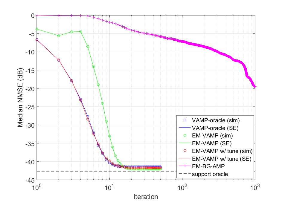
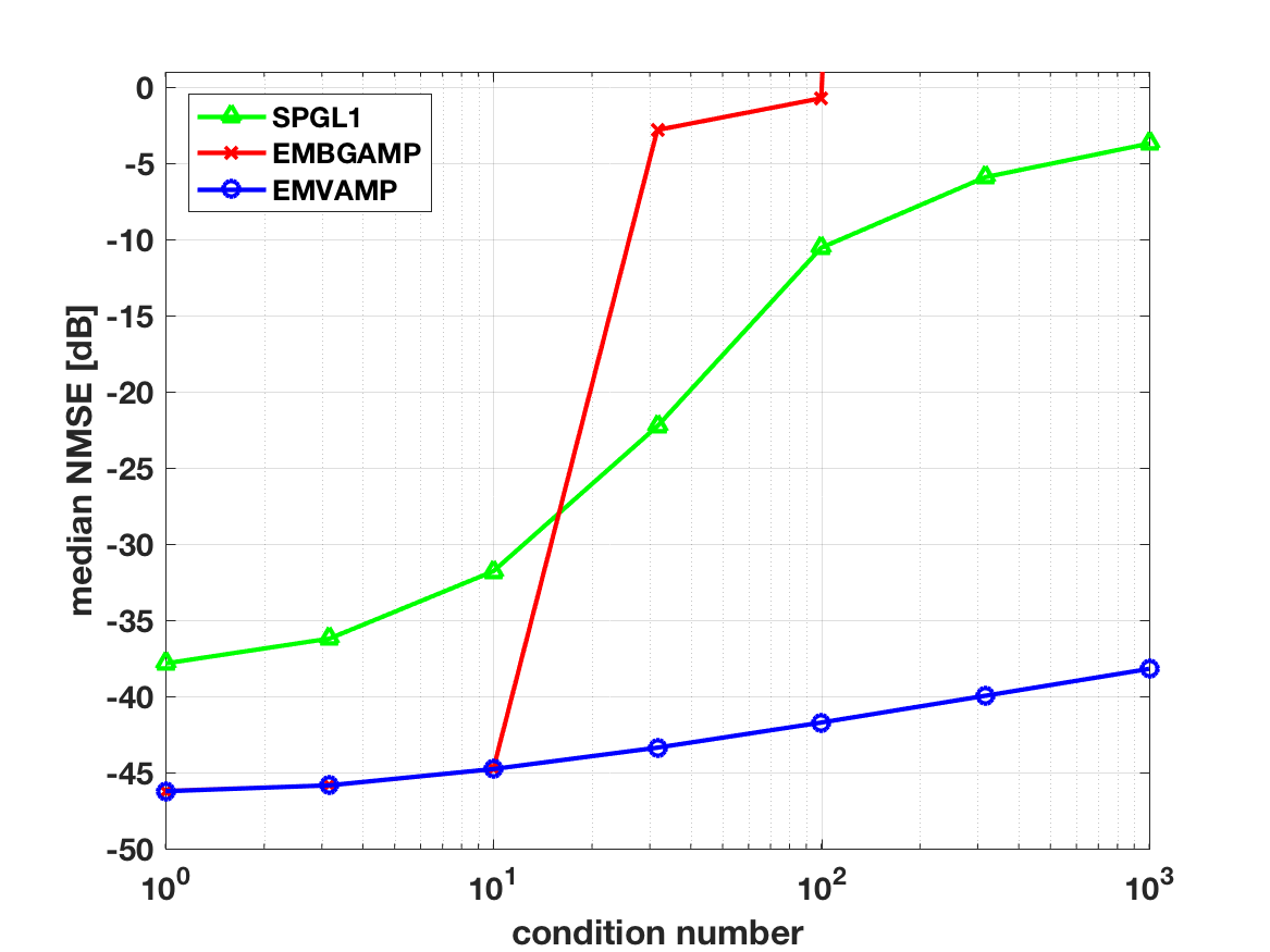
Figure 1: Numerical simulations. Left panel: Sparse signal recovery: NMSE versus iteration for condition number for a random matrix with a condition number $\kappa=100$. Right panel: NMSE for sparse image recovery (in AWGN at 40 dB SNR) as a function of the condition number $\kappa$.

We see several important features. First, for all variants of VAMP and EM-VAMP, the SE equations provide an excellent prediction of the per iteration performance of the algorithm. Second, consistent with the simulations in [22], the oracle VAMP converges remarkably fast ($\sim$ 10 iterations). Third, the performance of EM-VAMP with auto-tuning is virtually indistinguishable from oracle VAMP, suggesting that the parameter estimates are near perfect from the very first iteration. Fourth, the EM-VAMP method performs initially worse than the oracle-VAMP, but these errors are exactly predicted by the SE. Finally, all the VAMP and EM-VAMP algorithms exhibit much faster convergence than the EM-BG-AMP. In fact, consistent with observations in [21], EM-BG-AMP begins to diverge at higher condition numbers. In contrast, the VAMP algorithms are stable.

Compressed sensing image recovery

While the theory is developed on theoretical signal priors, we demonstrate that the proposed EM-VAMP algorithm can be effective on natural images. Specifically, we repeat the experiments in [31] for recovery of a sparse image. Again, see Appendix G for details including a picture of the image and the various reconstructions. An $N=256\times 256$ image of a satellite with $K=6678$ non-zero pixels is observed through a linear transform $\mathbf{A}=\mathop{\mathrm{diag}}(\mathbf{s})\mathbf{P}\mathbf{H}\mathop{\mathrm{diag}}(\mathbf{d})$ in AWGN at 40 dB SNR, where $\mathbf{H}$ is the fast Hadamard transform, $\mathbf{P}$ is a random sub-selection to $M<N$ measurements, $\mathbf{s}$ is a scaling to adjust the condition number, and $\mathbf{d}$ is a random $\pm 1$ vector. As in the previous example, the image vector $\mathbf{x}$ is modeled as sparse Bernoulli-Gaussian and the EM-VAMP algorithm is used to estimate the sparsity ratio, signal variance, and noise variance. The transform is set to have measurement ratio $M/N=0.5$. We see from the right panel of Fig. 1 that the EM-VAMP algorithm is able to reconstruct the images with improved performance over the standard basis pursuit denoising method SPGL1 [32] and the EM-BG-GAMP method from [15].

VI Conclusions

Due to its analytic tractability, computational simplicity, and potential for Bayes optimal inference, VAMP is a promising technique for statistical linear inverse problems. Importantly, it does not suffer the convergence issues of standard AMP methods when $\mathbf{A}$ is ill conditioned. However, a key challenge in using VAMP and related methods is the need to precisely specify the problem parameters. This work provides a rigorous foundation for analyzing VAMP in combination with various parameter adaptation techniques including EM. The analysis reveals that VAMP, with appropriate tuning, can also provide consistent parameter estimates under very general settings, thus yielding a powerful approach for statistical linear inverse problems.

Appendix A Adaptation with Finite-Dimensional Statistics

We provide two simple examples where the EM parameter update (47) can be computed from finite-dimensional statistics.

Finite number of parameter values

Suppose that ${\bm{\theta}}_{1}$ takes only a finite number of values ${\bm{\theta}}_{1}\in\{{\bm{\theta}}_{1}^{1},\ldots,{\bm{\theta}}_{1}^{L}\}$. Define the statistics,

$$\phi_{\ell}(r_{1},\gamma_{1},{\widehat{\bm{\theta}}}_{1}):=\mathbb{E}\left[\ln p(x|\theta_{1}^{\ell})|r_{1},\gamma_{1},{\widehat{\theta}}_{1}\right],$$

where the outer expectation is with respect to the belief estimate in $b_{1}(x|r_{1},\gamma_{1},{\widehat{\theta}}_{1})$ given in (5). Hence, the EM update in (47) is given by ${\widehat{\bm{\theta}}}_{1,k\!+\!1}={\bm{\theta}}_{1}^{\ell^{*}}$ where

$$\ell^{*}=\mathop{\mathrm{arg\,max}}_{\ell}\mu_{k,\ell},\quad\mu_{\ell}=\frac{1}{N}\sum_{n=1}^{N}\phi_{\ell}(r_{1k,n},\gamma_{1k},{\widehat{\bm{\theta}}}_{1k}).$$

Exponential family

Suppose that $p(\mathbf{x}|{\bm{\theta}}_{1})$ is given by an exponential family where the penalty function in (2) is given by $f_{1}(x,{\bm{\theta}}_{1})={\bm{\theta}}_{1}^{\text{\sf T}}\varphi(x)$ for some sufficient statistics $\varphi(x)\in{\mathbb{R}}^{d}$. Define the statistic,

$$\phi_{1}(r_{1},\gamma_{1},{\widehat{\bm{\theta}}}_{1}):=\mathbb{E}\left[\varphi(x)|r_{1},\gamma_{1},{\widehat{\bm{\theta}}}_{1}\right].$$

Then, the EM parameter update (47) can be computed by

$${\widehat{\bm{\theta}}}_{1,k\!+\!1}=\mathop{\mathrm{arg\,max}}_{{\bm{\theta}}_{1}}{\bm{\theta}}^{\text{\sf T}}\mu_{1}-\frac{1}{N}\ln Z_{1}({\bm{\theta}}_{1}),\quad\mu_{1}={\langle\phi_{1}(\mathbf{r}_{1k},\gamma_{1k},{\widehat{\bm{\theta}}}_{1k})\rangle}.$$

Hence, we see that the EM parameter update can be computed from a finite set of statistics.

Appendix B Proof of (11)

Using the SVD (9) and the equations for $\mathbf{Q}_{k}$ and $\widehat{\mathbf{x}}_{2k}$ in line 12 of Algorithm 1, we obtain

$$\mathbf{U}^{\text{\sf T}}(\mathbf{y}-\mathbf{A}\widehat{\mathbf{x}}_{2k})=\mathbf{U}^{\text{\sf T}}\mathbf{y}-\mathbf{S}\widehat{\mathbf{x}}_{2k}=\mathbf{U}^{\text{\sf T}}\mathop{\mathrm{diag}}\left[\frac{\gamma_{2k}}{\mathbf{s}^{2}{\widehat{\theta}}_{2k}+\gamma_{2k}}\right](\mathbf{S}\mathbf{q}_{2k}+{\bm{\xi}}).$$

Thus, the parameter estimate ${\widehat{\theta}}_{2,k\!+\!1}$ in line 18 is given by

$${\widehat{\theta}}_{2,k\!+\!1}^{-1}\stackrel{{\scriptstyle(a)}}{{=}}\frac{1}{N}\|\mathbf{U}^{\text{\sf T}}(\mathbf{y}-\mathbf{A}\widehat{\mathbf{x}}_{2k}\|^{2}+\frac{1}{N}\operatorname{tr}(\mathbf{A}^{\text{\sf T}}\mathbf{Q}_{k}\mathbf{A})$$

$$\stackrel{{\scriptstyle(b)}}{{=}}\frac{1}{N}\|\mathop{\mathrm{diag}}\left[\frac{\gamma_{2k}}{\mathbf{s}^{2}{\widehat{\theta}}_{2k}+\gamma_{2k}}\right](\mathbf{S}\mathbf{q}_{2k}+{\bm{\xi}})\|^{2}+\frac{1}{N}\operatorname{tr}\left[\mathbf{S}^{2}(\mathbf{S}^{2}{\widehat{\theta}}_{2k}+\gamma_{2k}\mathbf{I})^{-1}\right],$$

where (a) follows since $\mathbf{U}$ is unitary and therefore, $\|\mathbf{y}-\mathbf{A}\widehat{\mathbf{x}}_{2k}\|^{2}=\|\mathbf{U}^{\text{\sf T}}(\mathbf{y}-\mathbf{A}\widehat{\mathbf{x}}_{2k})\|^{2}$ and (b) follows from the SVD (9) and some simple manipulations. Therefore, if we define $\phi_{2}(\cdot)$ as in (12), we obtain (11).

Appendix C Convergence of Vector Sequences

We review some definitions from the Bayati and Montanari paper [12], since we will use the same analysis framework in this paper. Fix a dimension $r>0$, and suppose that, for each $N$, $\mathbf{x}(N)$ is a block vector of the form

$$\mathbf{x}(N)=(\mathbf{x}_{1}(N),\ldots,\mathbf{x}_{N}(N)),$$

where each component $\mathbf{x}_{n}(N)\in{\mathbb{R}}^{r}$. Thus, the total dimension of $\mathbf{x}(N)$ is $rN$. In this case, we will say that $\mathbf{x}(N)$ is a block vector sequence that scales with $N$ under blocks $\mathbf{x}_{n}(N)\in{\mathbb{R}}^{r}$. When $r=1$, so that the blocks are scalar, we will simply say that $\mathbf{x}(N)$ is a vector sequence that scales with $N$. Such vector sequences can be deterministic or random. In most cases, we will omit the notational dependence on $N$ and simply write $\mathbf{x}$.

Now, given $p\geq 1$, a function $\mathbf{f}:{\mathbb{R}}^{s}\rightarrow{\mathbb{R}}^{r}$ is called pseudo-Lipschitz of order $p$, if there exists a constant $C>0$ such that for all $\mathbf{x}_{1},\mathbf{x}_{2}\in{\mathbb{R}}^{s}$,

$$\|\mathbf{f}(\mathbf{x}_{1})-\mathbf{f}(\mathbf{x}_{2})\|\leq C\|\mathbf{x}_{1}-\mathbf{x}_{2}\|\left[1+\|\mathbf{x}_{1}\|^{p-1}+\|\mathbf{x}_{2}\|^{p-1}\right].$$

Observe that in the case $p=1$, pseudo-Lipschitz continuity reduces to the standard Lipschitz continuity.

Given $p\geq 1$, we will say that the block vector sequence $\mathbf{x}=\mathbf{x}(N)$ converges empirically with $p$-th order moments if there exists a random variable $X\in{\mathbb{R}}^{r}$ such that

1. $\mathbb{E}|X|^{p}<\infty$; and

2. for any scalar-valued pseudo-Lipschitz continuous function $f$ of order $p$,

   $$\lim_{N\rightarrow\infty}\frac{1}{N}\sum_{n=1}^{N}\mathbf{f}(\mathbf{x}_{n}(N))=\mathbb{E}\left[\mathbf{f}(X)\right].$$

Thus, the empirical mean of the components $\mathbf{f}(\mathbf{x}_{n}(N))$ converges to the expectation $\mathbb{E}(\mathbf{f}(X))$. In this case, with some abuse of notation, we will write

$$\lim_{N\rightarrow\infty}\left\{\mathbf{x}_{n}\right\}\stackrel{{\scriptstyle PL(p)}}{{=}}X,$$ (27)

where, as usual, we have omitted the dependence $\mathbf{x}_{n}=\mathbf{x}_{n}(N)$. Importantly, empirical convergence can be defined on deterministic vector sequences, with no need for a probability space. If $\mathbf{x}=\mathbf{x}(N)$ is a random vector sequence, we will often require that the limit (27) holds almost surely.

Finally, let $\mathbf{f}(\mathbf{x},\lambda)$ be a function on $\mathbf{x}\in{\mathbb{R}}^{s}$, dependent on some parameter vector $\lambda\in{\mathbb{R}}^{d}$. We say that $\mathbf{f}(\mathbf{x},\lambda)$ is uniformly pseudo-Lipschitz continuous of order $p$ in $\mathbf{x}$ at $\lambda={\overline{\lambda}}$ if there exists an open neighborhood $U$ of ${\overline{\lambda}}$, such that (i) $\mathbf{f}(\mathbf{x},\lambda)$ is pseudo-Lipschitz of order $p$ in $\mathbf{x}$ for all $\lambda\in U$; and (ii) there exists a constant $L$ such that

$$\|\mathbf{f}(\mathbf{x},\lambda_{1})-\mathbf{f}(\mathbf{x},\lambda_{2})\|\leq L\left(1+\|\mathbf{x}\|\right)|\lambda_{1}-\lambda_{2}|,$$ (28)

for all $\mathbf{x}\in{\mathbb{R}}^{s}$ and $\lambda_{1},\lambda_{2}\in U$. It can be verified that if $\mathbf{f}(\mathbf{x},\lambda)$ is uniformly pseudo-Lipschitz continuous of order $p$ in $\mathbf{x}$ at $\lambda={\overline{\lambda}}$, and $\lim_{N\rightarrow\infty}\lambda(N)={\overline{\lambda}}$, then

$$\lim_{N\rightarrow\infty}\mathbf{x}\stackrel{{\scriptstyle PL(p)}}{{=}}X\Longrightarrow\lim_{N\rightarrow\infty}\lim_{N\rightarrow\infty}\frac{1}{N}\sum_{n=1}^{N}\mathbf{f}(\mathbf{x}_{n}(N),\lambda(N))=\mathbb{E}\left[\mathbf{f}(X,{\overline{\lambda}})\right].$$

In the case when $\mathbf{f}(\cdot)$ is uniformly pseudo-Lipschitz continuous of order $p=1$, we will simply say $\mathbf{f}(\cdot)$ is uniformly Lipschitz.

Appendix D A General Convergence Result

The proof of Theorem 1 uses the following minor modification of the general convergence result in [22, Theorem 4]: We are given a dimension $N$, an orthogonal matrix $\mathbf{V}\in{\mathbb{R}}^{N\times N}$, an initial vector $\mathbf{u}_{0}\in{\mathbb{R}}^{N}$, and disturbance vectors $\mathbf{w}^{p},\mathbf{w}^{q}\in{\mathbb{R}}^{N}$. Then, we generate a sequence of iterates by the following recursion:

$$\mathbf{p}_{k} =\mathbf{V}\mathbf{u}_{k}$$ (29a)

$$\alpha_{1k} ={\langle\mathbf{f}_{p}^{\prime}(\mathbf{p}_{k},\mathbf{w}^{p},\gamma_{1k},{\widehat{\bm{\theta}}}_{1k})\rangle},\quad\mu_{1k}={\langle{\bm{\phi}}_{p}(\mathbf{p}_{k},\mathbf{w}^{p},\gamma_{1k},{\widehat{\bm{\theta}}}_{1k})\rangle}$$ (29b)

$$(C_{1k},\gamma_{2k},{\widehat{\bm{\theta}}}_{1,k\!+\!1}) =\Gamma_{1}(\gamma_{1k},\alpha_{1k},\mu_{1k},{\widehat{\bm{\theta}}}_{1k})$$ (29c)

$$\mathbf{v}_{k} =C_{1k}\left[\mathbf{f}_{p}(\mathbf{p}_{k},\mathbf{w}^{p},\gamma_{1k},{\widehat{\bm{\theta}}}_{1k})-\alpha_{1k}\mathbf{p}_{k}\right]$$ (29d)

$$\mathbf{q}_{k} =\mathbf{V}^{\text{\sf T}}\mathbf{v}_{k}$$ (29e)

$$\alpha_{2k} ={\langle\mathbf{f}_{q}^{\prime}(\mathbf{q}_{k},\mathbf{w}^{q},\gamma_{2k},{\widehat{\theta}}_{2k}))\rangle},\quad\mu_{2k}={\langle\phi_{q}(\mathbf{q}_{k},\mathbf{w}^{q},\gamma_{2k},{\widehat{\theta}}_{2k})\rangle}$$ (29f)

$$(C_{2k},\gamma_{1,k\!+\!1},{\widehat{\theta}}_{2,k\!+\!1}) =\Gamma_{1}(\gamma_{2k},\alpha_{2k},\mu_{2k},{\widehat{\theta}}_{2k})$$ (29g)

$$\mathbf{u}_{k\!+\!1} =C_{2k}\left[\mathbf{f}_{q}(\mathbf{q}_{k},\mathbf{w}^{q},\gamma_{2k},{\widehat{\theta}}_{2k})-\alpha_{2k}\mathbf{q}_{k}\right],$$ (29h)

which is initialized with some vector $\mathbf{u}_{0}$, scalar $\gamma_{10}$ and parameters ${\widehat{\theta}}_{0}=({\widehat{\bm{\theta}}}_{10},{\widehat{\theta}}_{20})$. Here, $\mathbf{f}_{p}(\cdot)$, $\mathbf{f}_{q}(\cdot)$, ${\bm{\phi}}_{p}(\cdot)$ and ${\bm{\phi}}_{q}(\cdot)$ are separable functions, meaning for all components $n$,

$$\begin{split}\left[\mathbf{f}_{p}(\mathbf{p},\mathbf{w}^{p},\gamma_{1},{\widehat{\bm{\theta}}}_{1})\right]_{n}=f_{p}(p_{n},w^{p}_{n},\gamma_{1},{\widehat{\bm{\theta}}}_{1})\quad\left[\mathbf{f}_{q}(\mathbf{q},\mathbf{w}^{q},\gamma_{2},{\widehat{\theta}}_{2})\right]_{n}=f_{q}(q_{n},w^{q}_{n},\gamma_{2},{\widehat{\theta}}_{2}),\\ \left[{\bm{\phi}}_{p}(\mathbf{p},\mathbf{w}^{p},\gamma_{1},{\widehat{\bm{\theta}}}_{1})\right]_{n}=\phi_{p}(p_{n},w^{p}_{n},\gamma_{1},{\widehat{\bm{\theta}}}_{1})\quad\left[{\bm{\phi}}_{q}(\mathbf{q},\mathbf{w}^{q},\gamma_{2},{\widehat{\theta}}_{2})\right]_{n}=\phi_{q}(q_{n},w^{q}_{n},\gamma_{2},{\widehat{\theta}}_{2}),\\ \end{split}$$ (30)

for functions $f_{p}(\cdot)$, $f_{q}(\cdot)$, $\phi_{q}(\cdot)$ and $\phi_{p}(\cdot)$. These functions may be vector-valued, but their dimensions are fixed and do not change with $N$. The functions $\Gamma_{i}(\cdot)$, $C_{i}(\cdot)$ and $T_{i}(\cdot)$ also have fixed dimensions with $C_{i}(\cdot)$ being scalar-valued.

Similar to the analysis of EM-VAMP, we consider the following large-system limit (LSL) analysis. We consider a sequence of runs of the recursions indexed by $N$. We model the initial condition $\mathbf{u}_{0}$ and disturbance vectors $\mathbf{w}^{p}$ and $\mathbf{w}^{q}$ as deterministic sequences that scale with $N$ and assume that their components converge empirically as

$$\lim_{N\rightarrow\infty}\{u_{0n}\}\stackrel{{\scriptstyle PL(2)}}{{=}}U_{0},\quad\lim_{N\rightarrow\infty}\{w^{p}_{n}\}\stackrel{{\scriptstyle PL(2)}}{{=}}W^{p},\quad\lim_{N\rightarrow\infty}\{w^{q}_{n}\}\stackrel{{\scriptstyle PL(2)}}{{=}}W^{q},$$ (31)

to random variables $U_{0}$, $W^{p}$ and $W^{q}$. We assume that the initial constants converges as

$$\lim_{N\rightarrow\infty}(\gamma_{10},{\widehat{\bm{\theta}}}_{10},{\widehat{\theta}}_{20})=(\overline{\gamma}_{10},{\overline{\bm{\theta}}}_{10},{\overline{\theta}}_{20})$$ (32)

for some values $(\overline{\gamma}_{10},{\overline{\bm{\theta}}}_{10},{\overline{\theta}}_{20})$. The matrix $\mathbf{V}\in{\mathbb{R}}^{N\times N}$ is assumed to be Haar distributed (i.e. uniform on the set of orthogonal matrices) and independent of $\mathbf{r}_{0}$, $\mathbf{w}^{p}$ and $\mathbf{w}^{q}$. Since $\mathbf{r}_{0}$, $\mathbf{w}^{p}$ and $\mathbf{w}^{q}$ are deterministic, the only randomness is in the matrix $\mathbf{V}$.

Under the above assumptions, define the SE equations

$$\overline{\alpha}_{1k} =\mathbb{E}\left[f_{p}^{\prime}(P_{k},W^{p},\overline{\gamma}_{1k},{\overline{\bm{\theta}}}_{1k})\right],\quad\overline{\mu}_{1k}=\mathbb{E}\left[\phi_{p}(P_{k},W^{p},\overline{\gamma}_{1k},{\overline{\bm{\theta}}}_{1k})\right]$$ (33a)

$$(\overline{C}_{1k},\overline{\gamma}_{2k},{\overline{\bm{\theta}}}_{1,k\!+\!1}) =\Gamma_{1}(\overline{\gamma}_{1k},\overline{\alpha}_{1k},\overline{\mu}_{1k},{\overline{\bm{\theta}}}_{1k})$$ (33b)

$$\tau_{2k} =\overline{C}_{1k}^{2}\left\{\mathbb{E}\left[f_{p}^{2}(P_{k},W^{p},\overline{\gamma}_{1k},{\overline{\bm{\theta}}}_{1k})\right]-\overline{\alpha}_{1k}^{2}\tau_{1k}\right\}$$ (33c)

$$\overline{\alpha}_{2k} =\mathbb{E}\left[f_{q}^{\prime}(Q_{k},W^{q},\overline{\gamma}_{2k},{\overline{\theta}}_{2k})\right],\quad\overline{\mu}_{1k}=\mathbb{E}\left[\phi_{q}(Q_{k},W^{q},\overline{\gamma}_{2k},{\overline{\theta}}_{2k})\right]$$ (33d)

$$\tau_{1,k\!+\!1} =\overline{C}_{2k}^{2}\left\{\mathbb{E}\left[f_{q}^{2}(Q_{k},W^{q},\overline{\gamma}_{2k},{\overline{\theta}}_{2k})\right]-\overline{\alpha}_{2k}^{2}\tau_{2k}\right\}$$ (33e)

which are initialized with the values in (32) and

$$\tau_{10}=\mathbb{E}U_{0}^{2},$$ (34)

where $U_{0}$ is the random variable in (31). In the SE equations (33), the expectations are taken with respect to random variables

$$P_{k}\sim{\mathcal{N}}(0,\tau_{1k}),\quad Q_{k}\sim{\mathcal{N}}(0,\tau_{2k}),$$

where $P_{k}$ is independent of $W^{p}$ and $Q_{k}$ is independent of $W^{q}$.

Theorem 3.

Consider the recursions (29) and SE equations (33) under the above assumptions. Assume additionally that, for all $k$:

1. For $i=1,2$, the function $\Gamma_{i}(\gamma_{i},\alpha_{i},\mu_{i},{\widehat{\theta}}_{i})$ is continuous at the points $(\overline{\gamma}_{ik},\overline{\alpha}_{ik},\overline{\mu}_{ik},{\overline{\bm{\theta}}}_{ik})$ from the SE equations;

2. The function $f_{p}(p,w^{p},\gamma_{1},{\widehat{\bm{\theta}}}_{1})$ and its derivative $f_{p}^{\prime}(p,w^{p},\gamma_{1})$ are uniformly Lipschitz continuous in $(p,w^{p})$ at $(\gamma_{1},{\bm{\theta}}_{1})=(\overline{\gamma}_{1k},{\overline{\bm{\theta}}}_{1k})$. The function $f_{q}(q,w^{q},\gamma_{2},{\widehat{\theta}}_{2})$ satisfies the analogous conditions.

3. The function $\phi_{p}(p,w^{p},\gamma_{1},{\widehat{\bm{\theta}}}_{1})$ is uniformly pseudo Lipschitz continuous of order 2 in $(p,w^{p})$ at $(\gamma_{1},{\bm{\theta}}_{1})=(\overline{\gamma}_{1k},{\overline{\bm{\theta}}}_{1k})$. The function $\phi_{q}(q,w^{q},\gamma_{2},{\widehat{\theta}}_{2})$ satisfies the analogous conditions.

Then,

1. For any fixed $k$, almost surely the components of $(\mathbf{w}^{p},\mathbf{p}_{0},\ldots,\mathbf{p}_{k})$ empirically converge as

   $$\lim_{N\rightarrow\infty}\left\{(w^{p}_{n},p_{0n},\ldots,p_{kn})\right\}\stackrel{{\scriptstyle PL(2)}}{{=}}(W^{p},P_{0},\ldots,P_{k}),$$ (35)

   where $W^{p}$ is the random variable in the limit (31) and $(P_{0},\ldots,P_{k})$ is a zero mean Gaussian random vector independent of $W^{p}$, with $\mathbb{E}(P_{k}^{2})=\tau_{1k}$. In addition, we have that

   $$\lim_{N\rightarrow\infty}(\alpha_{1k},\mu_{1k},\gamma_{2k},C_{1k},{\widehat{\bm{\theta}}}_{1,k\!+\!1})=(\overline{\alpha}_{1k},\overline{\mu}_{1k},\overline{\gamma}_{2k},\overline{C}_{1k},{\overline{\bm{\theta}}}_{1,k\!+\!1})$$ (36)

   almost surely.

2. For any fixed $k$, almost surely the components of $(\mathbf{w}^{q},\mathbf{q}_{0},\ldots,\mathbf{q}_{k})$ empirically converge as

   $$\lim_{N\rightarrow\infty}\left\{(w^{q}_{n},q_{0n},\ldots,q_{kn})\right\}\stackrel{{\scriptstyle PL(2)}}{{=}}(W^{q},Q_{0},\ldots,Q_{k}),$$ (37)

   where $W^{q}$ is the random variable in the limit (31) and $(Q_{0},\ldots,Q_{k})$ is a zero mean Gaussian random vector independent of $W^{q}$, with $\mathbb{E}(P_{k}^{2})=\tau_{2k}$. In addition, we have that

   $$\lim_{N\rightarrow\infty}(\alpha_{2k},\mu_{2k},\gamma_{1,k\!+\!1},C_{2k},{\widehat{\theta}}_{2,k\!+\!1})=(\overline{\alpha}_{2k},\overline{\mu}_{2k},\overline{\gamma}_{1,k\!+\!1},\overline{C}_{2k},{\overline{\theta}}_{2,k\!+\!1})$$ (38)

   almost surely.

Proof.

This is a minor modification of  [22, Theorem 4]. Indeed, the only change here is the addition of the terms $\mu_{ik}$ and ${\widehat{\bm{\theta}}}_{ik}$. Their convergence can be proven identically to that of $\alpha_{ik}$, $\gamma_{ik}$. For example, consider the proof of convergence $\alpha_{1k}\rightarrow\overline{\alpha}_{1k}$ in [22, Theorem 4]. This is proved as part of an induction argument where, in that part of the proof, the induction hypothesis is that (35) holds for some $k$ and (38) holds for $k\!-\!1$. Thus, $\gamma_{1k}\rightarrow\overline{\gamma}_{1k}$ and ${\widehat{\bm{\theta}}}_{1k}\rightarrow{\overline{\bm{\theta}}}_{1k}$ almost surely and $\lim_{N\rightarrow\infty}(\mathbf{p}_{k},\mathbf{w}^{p})\stackrel{{\scriptstyle PL(2)}}{{=}}(P_{k},W^{p})$. Hence, since $f_{p}(\cdot)$ is uniformly Lipschitz continuous,

$$\lim_{N\rightarrow\infty}\alpha_{1k}=\lim_{N\rightarrow\infty}{\langle\mathbf{f}_{p}(\mathbf{p}_{k},\mathbf{w}^{p},\gamma_{1k},{\widehat{\bm{\theta}}}_{1k})\rangle}=\mathbb{E}\left[f_{p}(P_{k},W^{p},\overline{\gamma}_{1k},{\overline{\bm{\theta}}}_{1k})\right]=\overline{\alpha}_{1k}.$$

Similarly, since we have assumed the uniform pseudo-Lipschitz continuity of $\phi_{p}(\cdot)$,

$$\lim_{N\rightarrow\infty}\mu_{1k}=\lim_{N\rightarrow\infty}{\langle{\bm{\phi}}_{p}(\mathbf{p}_{k},\mathbf{w}^{p},\gamma_{1k},{\widehat{\bm{\theta}}}_{1k})\rangle}=\mathbb{E}\left[\phi_{p}(P_{k},W^{p},\overline{\gamma}_{1k},{\overline{\bm{\theta}}}_{1k})\right]=\overline{\mu}_{1k}.$$

Thus, we have

$$\lim_{N\rightarrow\infty}(\gamma_{1k},\alpha_{1k},\mu_{1k},{\widehat{\bm{\theta}}}_{1k})=(\overline{\gamma}_{1k},\overline{\alpha}_{1k},\overline{\mu}_{1k},{\overline{\bm{\theta}}}_{1k}),$$

almost surely. Then, since $\Gamma_{1}(\cdot)$ is continuous, (29c) shows that

$$\lim_{N\rightarrow\infty}(C_{1k},\gamma_{2k},{\widehat{\bm{\theta}}}_{1,k\!+\!1})=(\overline{C}_{1k},\overline{\gamma}_{2k},{\overline{\bm{\theta}}}_{1,k\!+\!1})=\Gamma_{1}(\overline{\gamma}_{1k},\overline{\alpha}_{1k},\overline{\mu}_{1k},{\overline{\bm{\theta}}}_{1k}).$$

This proves (36). The modifications for the proof of (38) are similar. ∎

Appendix E Proof of Theorem 1

This proof is also a minor modification of the SE analysis of VAMP in [22, Theorem 1]. As in that proof, we need to simply rewrite the recursions in Algorithm 1 in the form (29) and apply the general convergence result in Theorem 3. To this end, define the error terms

$$\mathbf{p}_{k}:=\mathbf{r}_{1k}-\mathbf{x}^{0},\quad\mathbf{v}_{k}:=\mathbf{r}_{2k}-\mathbf{x}^{0},$$ (39)

and their transforms,

$$\mathbf{u}_{k}:=\mathbf{V}^{\text{\sf T}}\mathbf{p}_{k},\quad\mathbf{q}_{k}:=\mathbf{V}^{\text{\sf T}}\mathbf{v}_{k}.$$ (40)

Also, define the disturbance terms

$$\mathbf{w}^{q}:=({\bm{\xi}},\mathbf{s}),\quad\mathbf{w}^{p}:=\mathbf{x}^{0},\quad{\bm{\xi}}:=\mathbf{U}^{\text{\sf T}}\mathbf{w}.$$ (41)

Define the component-wise update functions

$$f_{p}(p,x^{0},\gamma_{1},{\widehat{\bm{\theta}}}_{1}):=g_{1}(p+x^{0},\gamma_{1},{\widehat{\bm{\theta}}}_{1})-x^{0},\quad f_{q}(q,(\xi,s),\gamma_{2},{\widehat{\theta}}_{2}):=\frac{{\widehat{\theta}}_{2}s\xi+\gamma_{2}q}{{\widehat{\theta}}_{2}s^{2}+\gamma_{2}}.$$ (42)

Also, define the adaptation functions,

$$\phi_{p}(p,x^{0},\gamma_{1},{\widehat{\bm{\theta}}}_{1}):=\phi_{1}(p+x^{0},\gamma_{1},{\widehat{\bm{\theta}}}_{1}),\quad\phi_{q}(q,(\xi,s),\gamma_{2},{\widehat{\theta}}_{2}):=\phi_{2}(q,\xi,s,\gamma_{2},{\widehat{\theta}}_{2}),$$ (43)

where $\phi_{1}(\cdot)$ is the statistic function in Algorithm 1 and $\phi_{2}(\cdot)$ are defined in (12).

With these definitions, we claim that the outputs satisfy the recursions:

$$\mathbf{p}_{k} =\mathbf{V}\mathbf{u}_{k}$$ (44a)

$$\alpha_{1k} ={\langle\mathbf{f}_{p}^{\prime}(\mathbf{p}_{k},\mathbf{x}^{0},\gamma_{1k},{\widehat{\bm{\theta}}}_{1})\rangle},\quad\gamma_{2k}=\frac{(1-\alpha_{1k})\gamma_{1k}}{\alpha_{1k}}$$ (44b)

$$\mathbf{v}_{k} =\frac{1}{1-\alpha_{1k}}\left[\mathbf{f}_{p}(\mathbf{p}_{k},\mathbf{x}^{0},\gamma_{1k})-\alpha_{1k}\mathbf{p}_{k}\right]$$ (44c)

$${\widehat{\bm{\theta}}}_{1,k\!+\!1} =T_{1}(\mu_{1k}),\quad\mu_{1k}={\langle\phi_{1}(\mathbf{v}_{k}+\mathbf{x}^{0},\gamma_{1k},{\widehat{\bm{\theta}}}_{1k})\rangle}$$ (44d)

$$\mathbf{q}_{k} =\mathbf{V}^{\text{\sf T}}\mathbf{v}_{k}$$ (44e)

$$\alpha_{2k} ={\langle\mathbf{f}_{q}^{\prime}(\mathbf{q}_{k},\mathbf{w}^{q},\gamma_{2k})\rangle},\quad\gamma_{1,k\!+\!1}=\frac{(1-\alpha_{2k})\gamma_{2k}}{\alpha_{2k}}$$ (44f)

$$\mathbf{u}_{k\!+\!1} =\frac{1}{1-\alpha_{2k}}\left[\mathbf{f}_{q}(\mathbf{q}_{k},\mathbf{w}^{q},\gamma_{2k})-\alpha_{2k}\mathbf{q}_{k}\right]$$ (44g)

$${\widehat{\theta}}_{2,k\!+\!1} =T_{2}(\mu_{2k}),\quad\mu_{2k}={\langle\phi_{2}(\mathbf{q}_{k},{\bm{\xi}},\gamma_{2k},{\widehat{\theta}}_{2k})\rangle}$$ (44h)

The fact that the updates in the modified Algorithm 1 satisfy (44a), (44b), (44e), (44f) can be proven exactly as in the proof of [22, Theorem 1]. The update (44d) follows from line 9 in Algorithm 1. The update (44h) follows from the definitions in (11).

Now, define

$$C_{ik}=\frac{1}{1-\alpha_{i}},$$

and the function,

$$\Gamma_{i}(\gamma_{i},\alpha_{i},\mu_{i},{\widehat{\bm{\theta}}}_{i})=\left(\frac{1}{1-\alpha_{i}},\frac{\gamma_{i}(1-\alpha_{i})}{\alpha_{i}},T_{i}(\mu_{i})\right),$$ (45)

the updates (44) are equivalent to the general recursions in (29). Also, the continuity assumptions (i)–(iii) in Theorem 3 are also easily verified. For example, for assumption (i), $\Gamma_{i}(\cdot)$ in (45) is continuous, since we have assumed that $\overline{\alpha}_{ik}\in(0,1)$ and $T_{i}(\mu_{i})$ is continuous at $\mu_{i}=\overline{\mu}_{ik}$.

For assumption (ii), the function $f_{p}(\cdot)$ in (42) is uniformly Lipschitz-continuous since we have assumed that $g_{1}(\cdot)$ is uniformly Lipschitz-continuous. Also, the SE equations (24a) and (24a) and the assumption that $\overline{\alpha}_{ik}>0$ show that $\overline{\gamma}_{ik}>0$ for all $i$ and $k$. In addition, the definition of $T_{2}(\cdot)$ and $\phi_{2}(\cdot)$ in (11) and (12) shows that ${\overline{\theta}}_{2k}>0$ as defined in (24e). Therefore, since $s$ is bounded in $[0,s_{\rm max}]$ and $\overline{\gamma}_{2k}>0$, ${\overline{\theta}}_{2k}>0$, we see that $f_{q}(\cdot)$ in (42) is uniformly Lipschitz-continuous.

Finally, for assumption (iii) in Theorem 3, the uniform pseudo-Lipschitz continuity of $\phi_{p}(\cdot)$ in (43) follows from the uniform pseudo-Lipschitz continuity assumption on $\phi_{1}(\cdot)$. Also, $\phi_{2}(\cdot)$ in (12) is uniformly pseudo-Lipschitz continuous of order 2 since $s\in[0,s_{\rm max}]$. Therefore, $\phi_{q}(\cdot)$ in (43) is also uniformly pseudo-Lipschitz continuous of order 2.

Hence, all the conditions of Theorem 3 are satisfied. The SE equations (24) then follow directly from the SE equations (33). This completes the proof.

Appendix F Variance Auto-Tuning Details and Proof of Theorem 2

F-A Proof of Theorem 2

To prove Theorem 2, we perform the variance auto-tuning adaptation as follows. Suppose the $X^{0}$ follows $X^{0}\sim p(\mathbf{x}|{\bm{\theta}}_{1}^{0})$ for some true parameter ${\bm{\theta}}_{1}^{0}$. Then, the SE analysis shows that the components of $\mathbf{r}_{1k}$ asymptotically behave as

$$R=X^{0}+P,\quad P={\mathcal{N}}(0,\tau_{1}),\quad X^{0}\sim p(\mathbf{x}|{\bm{\theta}}_{1}),$$ (46)

for ${\bm{\theta}}_{1}={\bm{\theta}}_{1}^{0}$ and some $\tau_{1}=\tau_{1k}$. The idea in variance auto-tuning is to jointly estimate $({\bm{\theta}}_{1},\tau_{1})$, say via maximum likelihood estimation,

$$({\widehat{\tau}}_{1k},{\widehat{\bm{\theta}}}_{1k})=\mathop{\mathrm{arg\,max}}_{\tau_{1},{\bm{\theta}}_{1}}\sum_{n=1}^{N}\ln p(r_{1k,n}|\tau_{1},{\bm{\theta}}_{1}),$$ (47)

where we use the notation $p(r_{1}|\tau_{1},{\bm{\theta}}_{1})$ to denote the density of $R$ under the model (46). We can then use both the parameter estimate ${\widehat{\bm{\theta}}}_{1k}$ and variance estimate ${\widehat{\tau}}_{1k}$ in the denoiser,

$$\widehat{\mathbf{x}}_{1k}=\mathbf{g}_{1}(\mathbf{r}_{1k},\gamma_{1k},{\widehat{\bm{\theta}}}_{1k}),\quad\gamma_{1k}={\widehat{\tau}}_{1k}^{-1}.$$ (48)

The parameter estimate (47) and precision estimate $\gamma_{1k}={\widehat{\tau}}_{1k}^{-1}$ would replace lines 9 and 14 in Algorithm 1. Since we are using the estimated precision ${\widehat{\tau}}_{1k}^{-1}$ from (47) instead of the predicted precision $\gamma_{1k}$, we call the estimation (47) with the estimate (48) variance auto-tuning.

Now suppose that statistic as in Definition 1 exists. By the inverse property, there must be a continuous mapping $T_{1}(\mu)$ such that for any $\tau_{1},{\bm{\theta}}_{1}$,

$$\mu_{1}=\mathbb{E}\left[\phi_{1}(R)|\tau_{1},{\bm{\theta}}_{1}\right]\Rightarrow T_{1}(\mu_{1})=(\tau_{1},{\bm{\theta}}_{1}).$$ (49)

Although the order of updates of ${\widehat{\bm{\theta}}}_{1k}$ and $\gamma_{1k}$ is slightly changed from Algorithm 1, we can apply an identical SE analysis and show that, in the LSL,

$$\lim_{N\rightarrow\infty}({\widehat{\tau}}_{1k},{\widehat{\bm{\theta}}}_{1k})=({\overline{\tau}}_{1k},{\widehat{\bm{\theta}}}_{1k})=T_{1}(\overline{\mu}_{1k}),\quad\overline{\mu}_{1k}=\mathbb{E}\left[\phi_{1}(R_{1})|\tau_{1k},{\bm{\theta}}_{1}^{0}\right],$$ (50)

where ${\bm{\theta}}_{1}^{0}$ is the true parameter. Comparing (49) and (50) we see that ${\overline{\bm{\theta}}}_{1k}={\bm{\theta}}_{1}^{0}$ and ${\overline{\tau}}_{1k}=\tau_{1k}$. This proves Theorem 2.

F-B Auto-Tuning Details

The auto-tuning above requires solving a joint ML estimation (47). We describe a simple approximate method for this estimation using EM. First, we rewrite the ML estimation in (47) as

$$({\widehat{\tau}}_{1},{\widehat{\bm{\theta}}}_{1})=\mathop{\mathrm{arg\,max}}_{\tau_{1},{\bm{\theta}}_{1}}\ln p(\mathbf{r}_{1}|\tau_{1},{\bm{\theta}}_{1}),$$ (51)

where we have dropped the dependence on the iteration $k$ to simplify the notation and we have used the notation $p(\mathbf{r}_{1}|\tau_{1},{\bm{\theta}}_{1}):=\prod_{n}p(r_{1n}|\tau_{1},{\bm{\theta}}_{1})$. It will be more convenient to precisions rather than variances, so we rewrite (52),

$$({\widehat{\gamma}}_{1},{\widehat{\bm{\theta}}}_{1})=\mathop{\mathrm{arg\,max}}_{\gamma_{1},{\bm{\theta}}_{1}}\ln p(\mathbf{r}_{1}|\gamma_{1},{\bm{\theta}}_{1}),$$ (52)

where $\gamma_{1}=1/\tau_{1}$. Treating $\mathbf{x}$ as latent vector, the EM procedure for the ML estimate (52) performs updates $({\widehat{\gamma}}_{1}^{\rm old},{\widehat{\bm{\theta}}}_{1}^{\rm old})\mapsto({\widehat{\gamma}}_{1}^{\rm new},{\widehat{\bm{\theta}}}_{1}^{\rm new})$ given by

$$({\widehat{\gamma}}_{1}^{\rm new},{\widehat{\bm{\theta}}}_{1}^{\rm new})=\mathop{\mathrm{arg\,max}}_{\gamma_{1},{\bm{\theta}}_{1}}\mathbb{E}\left[\ln p(\mathbf{x},\mathbf{r}_{1}|\gamma_{1},{\bm{\theta}}_{1})\mid\mathbf{r}_{1},\gamma_{1}^{\rm old},{\widehat{\bm{\theta}}}_{1}^{\rm old}\right],$$ (53)

where the expectation is with respect to the posterior density, $p(\mathbf{x}|\mathbf{r}_{1},{\widehat{\gamma}}_{1}^{\rm old},{\widehat{\bm{\theta}}}_{1}^{\rm old})$. But, this posterior density is precisely the belief estimate $b_{i}(\mathbf{x}|\mathbf{r}_{1},\gamma_{i}^{\rm old},{\widehat{\theta}}_{1}^{\rm old})$. Now, under the model (46), the log likelihood $\ln p(\mathbf{x},\mathbf{r}_{1}|\gamma,{\bm{\theta}}_{1})$ is given by

$$\ln p(\mathbf{x},\mathbf{r}_{1}|\gamma_{1},{\bm{\theta}}_{1})=\ln p(\mathbf{r}|\mathbf{x},\gamma_{1})+\ln p(\mathbf{x}|{\bm{\theta}}_{1})$$

$$=-\frac{\gamma_{1}}{2}\|\mathbf{r}-\mathbf{x}\|^{2}+\frac{N}{2}\ln(\gamma_{1})+\ln p(\mathbf{x}|{\bm{\theta}}_{1}).$$

Thus, the maximization in (53) with respect to $\gamma_{1}$ is

$$\left({\widehat{\gamma}}_{1}^{\rm new}\right)^{-1}=\frac{1}{N}\mathbb{E}\left[\|\mathbf{x}-\mathbf{r}_{1}\|^{2}\mid|{\widehat{\tau}}_{1}^{\rm old},{\widehat{\bm{\theta}}}_{1}^{\rm old}\right]=\frac{1}{N}\|\widehat{\mathbf{x}}_{1}-\mathbf{r}_{1}\|^{2}+\eta_{1}^{-1},$$ (54)

where

$$\widehat{\mathbf{x}}_{1}=\mathbb{E}\left[\mathbf{x}\mid\mathbf{r}_{1},{\widehat{\gamma}}_{1}^{\rm old},{\widehat{\bm{\theta}}}_{1}^{\rm old}\right],\quad\eta_{1}^{-1}=\frac{1}{N}\operatorname{tr}\operatorname{Cov}\left[\mathbf{x}\mid\mathbf{r}_{1},{\widehat{\gamma}}_{1}^{\rm old},{\widehat{\bm{\theta}}}_{1}^{\rm old}\right].$$

The maximization in (53) with respect to ${\bm{\theta}}_{1}$ is

$${\widehat{\bm{\theta}}}_{1}^{\rm new}=\mathop{\mathrm{arg\,max}}_{{\bm{\theta}}_{1}}\mathbb{E}\left[p(\mathbf{x}|{\bm{\theta}}_{1})|\mathbf{r}_{1},\gamma_{1}^{\rm old},{\widehat{\bm{\theta}}}_{1}^{\rm old}\right],$$

which is precisely the EM update (7) with the current parameter estimates. Thus, the auto-tuning estimation can be performed by repeatedly performing updates

$$\widehat{\mathbf{x}}_{1} =\mathbb{E}\left[\mathbf{x}\mid\mathbf{r}_{1},{\widehat{\gamma}}_{1}^{\rm old},{\widehat{\bm{\theta}}}_{1}^{\rm old}\right],\quad\eta_{1}^{-1}=\frac{1}{N}\operatorname{tr}\operatorname{Cov}\left[\mathbf{x}\mid\mathbf{r}_{1},{\widehat{\gamma}}_{1}^{\rm old},{\widehat{\bm{\theta}}}_{1}^{\rm old}\right],$$ (55a)

$$\left({\widehat{\gamma}}_{1}^{\rm new}\right)^{-1} =\frac{1}{N}\|\widehat{\mathbf{x}}_{1}-\mathbf{r}_{1}\|^{2}+\eta_{1}^{-1}$$ (55b)

$${\widehat{\bm{\theta}}}_{1}^{\rm new} =\mathop{\mathrm{arg\,max}}_{{\bm{\theta}}_{1}}\mathbb{E}\left[p(\mathbf{x}|{\bm{\theta}}_{1})|\mathbf{r}_{1},\gamma_{1}^{\rm old},{\widehat{\bm{\theta}}}_{1}^{\rm old}\right].$$ (55c)

Thus, each iteration of the auto-tuning involves calling the denoiser (55a) at the current estimate; updating the variance from the denoiser error (55b); and updating the parameter estimate via an EM-type update (55c).

F-C Consistent Estimation of $\theta_{2}$

We show how we can perform a similar ML estimation as in Section IV for estimating the noise precision $\theta_{2}$ and error variance $\tau_{2}$ at the output. Suppose that the true noise precision is $\theta_{2}=\theta_{2}^{0}$. Define

$$\mathbf{z}_{k}=\mathbf{S}\mathbf{V}^{\text{\sf T}}\mathbf{r}_{2k}-\mathbf{U}^{\text{\sf T}}\mathbf{y}.$$ (56)

Then,

$$\mathbf{z}_{k}\stackrel{{\scriptstyle(a)}}{{=}}\mathbf{S}\mathbf{V}^{\text{\sf T}}\mathbf{r}_{2k}-\mathbf{U}^{\text{\sf T}}(\mathbf{A}\mathbf{x}^{0}+\mathbf{w})\stackrel{{\scriptstyle(b)}}{{=}}\mathbf{S}\mathbf{q}_{k}+{\bm{\xi}},$$

where (a) follows from (13) and (b) follows from (9) and (10). From Theorem 1 and the limit (23), $\mathbf{z}_{k}$ converge empirically to a random variable $Z_{k}$ given by

$$Z_{k}=SQ_{k}+\Xi,\quad Q_{k}\sim{\mathcal{N}}(0,\tau_{2}),\quad\Xi\sim{\mathcal{N}}(0,\theta_{2}^{-1}),$$ (57)

where $(\theta_{2},\tau_{2})=(\theta_{2}^{0},\tau_{2k})$ are the true noise precision and error variance. Similar to the auto-tuning of ${\bm{\theta}}_{1}$ in Section IV, we can attempt to estimate $(\tau_{2},\theta_{2})$ via ML estimation,

$$({\widehat{\tau}}_{2k},{\widehat{\theta}}_{2k})=\mathop{\mathrm{arg\,max}}_{\tau_{2},\theta_{2}}\frac{1}{N}\sum_{n=1}^{N}\ln p(z_{k,n}|\theta_{2},\tau_{2},s_{n}),$$ (58)

where $p(z|\theta_{2},\tau_{2},s)$ is the density of the random variable $Z_{k}$ in the model (57). Recall that the singular values $s_{n}$ are known to the estimator. Then, using these estimates, we perform the estimate of $\widehat{\mathbf{x}}_{2k}$ in line 12 of Algorithm 1 using the estimated precision $\gamma_{2k}=1/{\widehat{\tau}}_{2k}$.

To analyze this estimator rigorously, we make the simplifying assumption that the random variable, $S$, representing the distribution of singular values, is discrete. That is, there are a finite number of values $a_{1},\cdots,a_{L}$ and probabilities $p_{1},\ldots,p_{L}$ such that

$$\Pr(S^{2}=a_{\ell})=p_{\ell}.$$

Then, given vectors $\mathbf{z}_{k}$ and $\mathbf{s}$, define the $2L$ statistics

$$\phi_{\ell 0}(z,s)=\mathbbm{1}_{\{{s^{2}=a_{\ell}}\}},\quad\phi_{\ell 1}(z,s)=z^{2}\mathbbm{1}_{\{{s^{2}=a_{\ell}}\}},\quad\ell=1,\ldots,L,$$

and their empirical averages at time $k$,

$$\mu_{\ell 0}={\langle\mathbbm{1}_{\{{s_{n}^{2}=a_{\ell}}\}}\rangle},\quad\mu_{\ell 1}={\langle z_{k,n}^{2}\mathbbm{1}_{\{{s_{n}^{2}=a_{\ell}}\}}\rangle}.$$

Then, the ML estimate in (58) can be rewritten as

$$({\widehat{\tau}}_{2k},{\widehat{\theta}}_{2k})=\mathop{\mathrm{arg\,min}}_{\tau_{2},\theta_{2}}J(\tau_{2},\theta_{2}),$$ (59)

where the objective function is

$$J(\tau_{2},\theta_{2}):==\frac{1}{N}\sum_{n=1}^{N}\left[\frac{z_{k,n}^{2}}{s_{n}^{2}\tau_{2}+\theta_{2}^{-1}}+\ln(s_{n}^{2}\tau_{2}+\theta_{2}^{-1})\right]=\sum_{\ell=1}^{L}\left[\frac{\mu_{\ell 1}}{a_{\ell}\tau_{2}+\theta_{2}^{-1}}+\mu_{\ell 0}\ln(a_{\ell}\tau_{2}+\theta_{2}^{-1})\right].$$ (60)

Hence, we can compute the ML estimate (58) from an objective function computed from the $2L$ statistics, $\mu_{\ell 0},\mu_{\ell 1}$, $\ell=1,\ldots,L$.

To prove consistency of the ML estimate, first note that the SE analysis shows that $\mu_{\ell 0}\rightarrow\overline{\mu}_{\ell 0}$ and $\mu_{\ell 1}\rightarrow\overline{\mu}_{\ell 1}$ where the limits are given by

$$\overline{\mu}_{\ell 0} =\mathbb{E}\left[\phi_{\ell 0}(Z,S)\right]=P(S^{2}=a_{\ell})=p_{\ell},$$

$$\overline{\mu}_{\ell 1} =\mathbb{E}\left[\phi_{\ell 1}(Z,S)\right]=\mathbb{E}(Z^{2}|S^{2}=a_{\ell})P(S^{2}=a_{\ell})=p_{\ell}\left[a_{\ell}\tau_{2k}+(\theta_{2}^{0})^{-1}\right],$$

where $(\tau_{2k},\theta_{2}^{0})$ are the true values of $(\tau_{2},\theta_{2})$. Hence, the objective function in (60) will converge to

$$\lim_{N\rightarrow\infty}J(\tau_{2},\theta_{2})=\sum_{\ell=1}^{L}p_{\ell}\left[\frac{a_{\ell}\tau_{2}^{0}+(\theta_{2}^{0})^{-1}}{a_{\ell}\tau_{2}+\theta_{2}^{-1}}+\mu_{\ell 0}\ln(a_{\ell}\tau_{2}+\theta_{2}^{-1})\right].$$ (61)

Now, for any $y>0$,

$$\mathop{\mathrm{arg\,min}}_{x>0}\frac{y}{x}+\ln(x)=y.$$

Thus, the minima of (61) will occur at

$$({\overline{\tau}}_{2k},{\overline{\theta}}_{2k}):=(\tau_{2k},{\bm{\theta}}_{1}^{0}).$$ (62)

It can also be verified that this minima is unique provided that there are at least two different values $a_{\ell}$ with non-zero probabilities $p_{\ell}$. That is, we require that $S^{2}$ is not constant. In this case, one can show that the mapping from the statistics $\{\mu_{\ell 0},\mu_{\ell 1})\}$ to the ML estimates $({\widehat{\tau}}_{2k},{\widehat{\theta}}_{2k})$ in (59) is continuous at the limiting values $\{\overline{\mu}_{\ell 0},\overline{\mu}_{\ell 1})\}$. Hence, from the SE analysis, we obtain that $({\widehat{\tau}}_{2k},{\widehat{\theta}}_{2k})\rightarrow({\overline{\tau}}_{2k},{\overline{\theta}}_{2k})=(\tau_{2k},\theta_{2}^{0})$, in (62). We have proven the following.

Theorem 4.

Under the assumptions of Theorem 1, let $\theta_{2}^{0}$ denote the true noise precision and $\tau_{2k}$ be the true error variance for some iteration $k$. Suppose that the random variable $S^{2}$ representing the squared singular values is discrete and non-constant. Then, there exists a finite set of statistics $\phi_{\ell 0}(z_{n},s_{n})$ and $\phi_{\ell 1}(z_{n},s_{n})$ and parameter selection rule such that the estimates $({\widehat{\tau}}_{2k},{\widehat{\theta}}_{2k})$ are asymptotically consistent in that

$$\lim_{N\rightarrow\infty}({\widehat{\tau}}_{2k},{\widehat{\theta}}_{2k})=(\tau_{2k},\theta_{1}^{0}),$$

almost surely.

Appendix G Simulation Details

Sparse signal recovery

To model the sparsity, $\mathbf{x}$ is drawn as an i.i.d. Bernoulli-Gaussian (i.e., spike and slab) prior,

$$p(x_{n}|{\bm{\theta}}_{1})=(1-\beta_{x})\delta(x_{n})+\beta_{x}{\mathcal{N}}(x_{n};\mu_{x},\tau_{x}),$$ (63)

where parameters ${\bm{\theta}}_{1}=\{\beta_{x},\mu_{x},\tau_{x}\}$ represent the sparsity rate $\beta_{x}\in(0,1]$, the active mean $\mu_{x}\in{\mathbb{R}}$, and the active variance $\tau_{x}>0$. Following [17, 18], we constructed $\mathbf{A}\in{\mathbb{R}}^{M\times N}$ from the SVD $\mathbf{A}=\mathbf{U}\mathbf{S}\mathbf{V}^{\text{\sf T}}$, whose orthogonal matrices $\mathbf{U}$ and $\mathbf{V}$ were drawn uniformly with respect to the Haar measure and whose singular values $s_{i}$ were constructed as a geometric series, i.e., $s_{i}/s_{i-1}=\alpha~{}\forall i>1$, with $\alpha$ and $s_{1}$ chosen to achieve a desired condition number $\kappa=s_{1}/s_{\min(M,N)}$ as well as $\|\mathbf{A}\|_{F}^{2}=N$. This matrix model provides a good test for the stability of AMP methods since it is known that the matrix having a high condition number is the main failure mechanism in AMP [17]. Recovery performance was assessed using normalized MSE (NMSE) $\|\widehat{\mathbf{x}}-\mathbf{x}\|^{2}/\|\mathbf{x}\|^{2}$ averaged over $100$ independent draws of $\mathbf{A}$, $\mathbf{x}$, and $\mathbf{w}$.

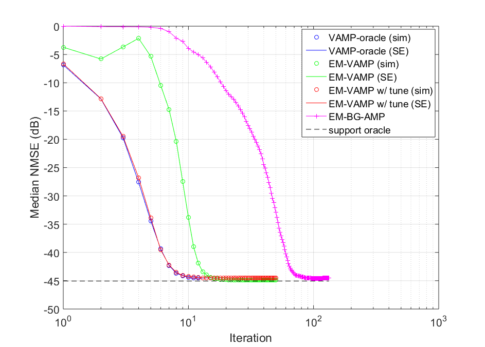
Figure 2: Sparse signal recovery: Plotted are the NMSE for various algorithms with a condition number of $\kappa=10$.

The left panel of figure 1 shows the NMSE versus iteration for various algorithms under $M=512$, $N=1024$, $\beta_{x}=0.1$, $\mu_{x}=0$, and $(\tau_{x},\theta_{2})$ giving a signal-to-noise ratio of $40$ dB at a condition number of $\kappa=100$. The identical simulation is shown in Fig. 2. The trends in both figures are discussed in the main text. The EM-VAMP algorithms were initialized with $\beta_{x}=(M/2)/N$, $\tau_{x}=\|\mathbf{y}\|^{2}/\|\mathbf{A}\|_{F}^{2}\beta_{x}$, $\mu_{x}=0$, and $\theta_{2}^{-1}=M^{-1}\|\mathbf{y}\|^{2}$. Four methods are compared: (i) VAMP-oracle, which is VAMP under perfect knowledge of ${\bm{\theta}}=\{\tau_{w},\beta_{x},\mu_{x},\tau_{x}\}$; (ii) EM-VAMP from [21]; (iii) EM-VAMP with auto-tuning described in Section IV; (iv) the EM-BG-AMP algorithm from [15] with damping from [18]; and (v) a lower bound obtain by an oracle estimator that knows the support of the vector $\mathbf{x}$. For algorithms (i)–(iii), we have plotted both the simulated median NMSE as well as the state-evolution (SE) predicted performance.

Sparse image recovery

The true image is shown in the top left panel of Fig. 3 and can be seen to be sparse in the pixel domain. Three image recovery algorithms were tested: (i) the EM-BG-AMP algorithm [15] with damping from [18]; (ii) basis pursuit denoising using SPGL1 as described in [32]; and (iii) EM-VAMP with auto-tuning described in Section IV. For the EM-BG-AMP and EM-VAMP algorithms, the BG model was used, as before. SPGL1 was run in “BPDN mode," which solves $\min_{\mathbf{x}}\|\mathbf{x}\|_{1}$ subject to $\|\mathbf{y}-\mathbf{A}\mathbf{x}\|\leq\sigma$ for true noise variance $\sigma^{2}$. All algorithms are run over 51 trials, with the median value plotted in Fig. 1. While the EM-VAMP theory provides convergence guarantees when the true distribution fits the model class and in the large-system limit, we found some damping was required on finite-size, real images that are not generated from the assumed prior. In this experiment, to obtain stable convergence, the EM-VAMP algorithm was aggressively damped as described in [22], using a damping ratio of 0.5 for the first- and second-order terms.

The computation times as a function of condition number $\kappa$ are shown in Fig. 4. All three methods benefit from the fact that the matrix $\mathbf{A}$ has a fast implementation. In addition, for EM-VAMP, the matrix has an easily computable SVD. The figure shows that the EM-VAMP algorithm achieves dramatically faster performance at high condition numbers – approximately 10 times faster than either EM-BG-AMP or SPGL1. The various panels of Fig. 3 show the images recovered by each algorithm at condition number $\kappa=100$ for the realization that achieved the median value in Fig. 1 (right panel).

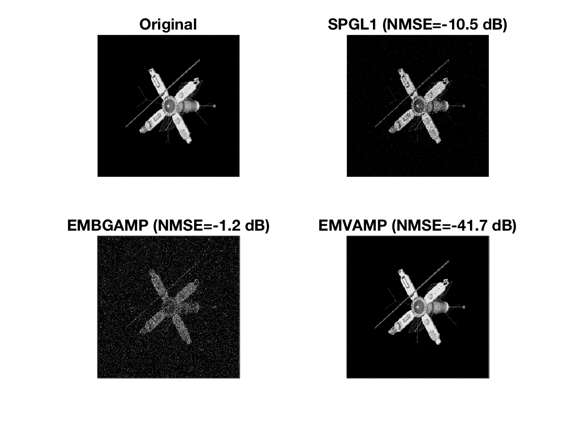
Figure 3: Sparse image recovery: Original ’satellite’ image as used in [18] along with the median-NMSE recovered images for the various algorithms at measurement ratio $M/N=0.5$, condition number $\kappa=100$, and 40 dB SNR.

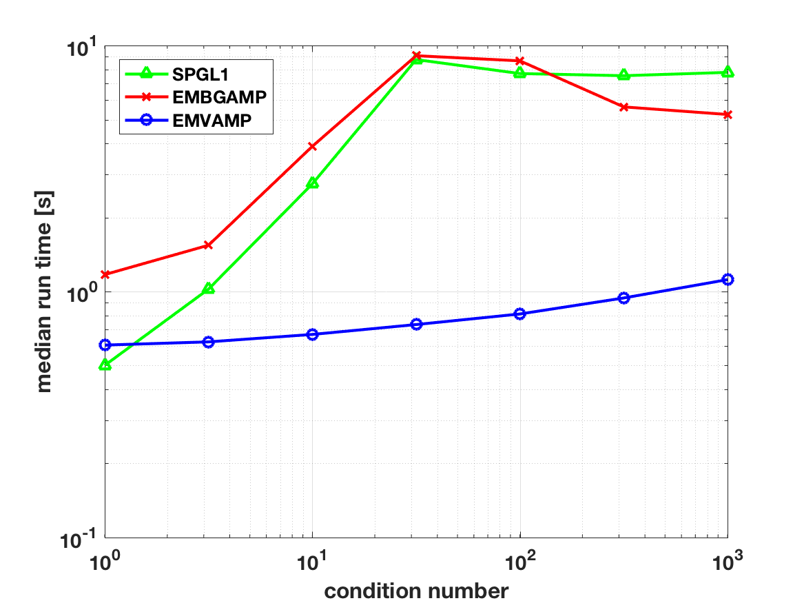
Figure 4: Computation time versus condition number for various algorithms in the satellite image recovery problem.

References

- [1] D. L. Donoho, A. Maleki, and A. Montanari, “Message-passing algorithms for compressed sensing,” Proc. Nat. Acad. Sci., vol. 106, no. 45, pp. 18 914–18 919, Nov. 2009.
- [2] S. Rangan, “Generalized approximate message passing for estimation with random linear mixing,” in Proc. IEEE Int. Symp. Inform. Theory, Saint Petersburg, Russia, Jul.–Aug. 2011, pp. 2174–2178.
- [3] T. P. Minka, “A family of algorithms for approximate Bayesian inference,” Ph.D. dissertation, Dept. Comp. Sci. Eng., MIT, Cambridge, MA, 2001.
- [4] A. K. Fletcher, S. Rangan, L. Varshney, and A. Bhargava, “Neural reconstruction with approximate message passing (NeuRAMP),” in Proc. Neural Information Process. Syst., Granada, Spain, Dec. 2011, pp. 2555–2563.
- [5] P. Schniter, “A message-passing receiver for BICM-OFDM over unknown clustered-sparse channels,” IEEE J. Sel. Topics Signal Process., vol. 5, no. 8, pp. 1462–1474, Dec. 2011.
- [6] S. Som and P. Schniter, “Compressive imaging using approximate message passing and a Markov-tree prior,” IEEE Trans. Signal Process., vol. 60, no. 7, pp. 3439–3448, Jul. 2012.
- [7] J. Ziniel and P. Schniter, “Dynamic compressive sensing of time-varying signals via approximate message passing,” IEEE Trans. Signal Process., vol. 61, no. 21, pp. 5270–5284, Nov. 2013.
- [8] J. P. Vila and P. Schniter, “An empirical-Bayes approach to recovering linearly constrained non-negative sparse signals,” IEEE Trans. Signal Process., vol. 62, no. 18, pp. 4689–4703, Sep. 2014.
- [9] P. Schniter and S. Rangan, “Compressive phase retrieval via generalized approximate message passing,” IEEE Trans. Signal Process., vol. 63, no. 4, pp. 1043–1055, 2015.
- [10] J. Ziniel, P. Schniter, and P. Sederberg, “Binary linear classification and feature selection via generalized approximate message passing,” IEEE Trans. Signal Process., vol. 63, no. 8, pp. 2020–2032, 2015.
- [11] A. K. Fletcher and S. Rangan, “Scalable inference for neuronal connectivity from calcium imaging,” in Proc. Neural Information Processing Systems, 2014, pp. 2843–2851.
- [12] M. Bayati and A. Montanari, “The dynamics of message passing on dense graphs, with applications to compressed sensing,” IEEE Trans. Inform. Theory, vol. 57, no. 2, pp. 764–785, Feb. 2011.
- [13] A. Javanmard and A. Montanari, “State evolution for general approximate message passing algorithms, with applications to spatial coupling,” Information and Inference, vol. 2, no. 2, pp. 115–144, 2013.
- [14] F. Krzakala, M. Mézard, F. Sausset, Y. Sun, and L. Zdeborová, “Statistical-physics-based reconstruction in compressed sensing,” Physical Review X, vol. 2, no. 2, p. 021005, 2012.
- [15] J. P. Vila and P. Schniter, “Expectation-maximization Gaussian-mixture approximate message passing,” IEEE Trans. Signal Process., vol. 61, no. 19, pp. 4658–4672, 2013.
- [16] U. S. Kamilov, S. Rangan, A. K. Fletcher, and M. Unser, “Approximate message passing with consistent parameter estimation and applications to sparse learning,” IEEE Trans. Inform. Theory, vol. 60, no. 5, pp. 2969–2985, Apr. 2014.
- [17] S. Rangan, P. Schniter, and A. Fletcher, “On the convergence of approximate message passing with arbitrary matrices,” in Proc. IEEE Int. Symp. Inform. Theory, Jul. 2014, pp. 236–240.
- [18] J. Vila, P. Schniter, S. Rangan, F. Krzakala, and L. Zdeborová, “Adaptive damping and mean removal for the generalized approximate message passing algorithm,” in Proc. IEEE Int. Conf. Acoust., Speech, and Signal Process., 2015, pp. 2021–2025.
- [19] A. Manoel, F. Krzakala, E. W. Tramel, and L. Zdeborová, “Swept approximate message passing for sparse estimation,” in Proc. ICML, 2015, pp. 1123–1132.
- [20] S. Rangan, A. K. Fletcher, P. Schniter, and U. S. Kamilov, “Inference for generalized linear models via alternating directions and Bethe free energy minimization,” IEEE Trans. Inform. Theory, vol. 63, no. 1, pp. 676–697, 2017.
- [21] A. K. Fletcher and P. Schniter, “Learning and free energies for vector approximate message passing,” arXiv:1602.08207, 2016.
- [22] S. Rangan, P. Schniter, and A. K. Fletcher, “Vector approximate message passing,” arXiv:1610.03082, 2016.
- [23] M. Opper and O. Winther, “Expectation consistent free energies for approximate inference,” in Proc. NIPS, 2004, pp. 1001–1008.
- [24] ——, “Expectation consistent approximate inference,” J. Mach. Learning Res., vol. 1, pp. 2177–2204, 2005.
- [25] A. K. Fletcher, M. Sahraee-Ardakan, S. Rangan, and P. Schniter, “Expectation consistent approximate inference: Generalizations and convergence,” in Proc. IEEE Int. Symp. Inform. Theory, 2016, pp. 190–194.
- [26] K. Takeuchi, “Rigorous dynamics of expectation-propagation-based signal recovery from unitarily invariant measurements,” arXiv:1701.05284, 2017.
- [27] A. M. Tulino, G. Caire, S. Verdú, and S. Shamai, “Support recovery with sparsely sampled free random matrices,” IEEE Trans. Inform. Theory, vol. 59, no. 7, pp. 4243–4271, 2013.
- [28] J. Barbier, M. Dia, N. Macris, and F. Krzakala, “The mutual information in random linear estimation,” arXiv:1607.02335, 2016.
- [29] G. Reeves and H. D. Pfister, “The replica-symmetric prediction for compressed sensing with Gaussian matrices is exact,” in Proc. IEEE ISIT, 2016.
- [30] T. Heskes, O. Zoeter, and W. Wiegerinck, “Approximate expectation maximization,” NIPS, vol. 16, pp. 353–360, 2004.
- [31] J. P. Vila and P. Schniter, “An empirical-Bayes approach to recovering linearly constrained non-negative sparse signals,” IEEE Trans. Signal Process., vol. 62, no. 18, pp. 4689–4703, 2014.
- [32] E. Van Den Berg and M. P. Friedlander, “Probing the Pareto frontier for basis pursuit solutions,” SIAM J. Sci. Comput., vol. 31, no. 2, pp. 890–912, 2008.