The effects on a core collapse of changes in the number and size of turbulent modes of velocity

Consideramos 28 simulaciones de partículas diseñadas para comparar el colapso gravitacional de un núcleo de gas uniforme y esféricamente simétrico, en el cual dos tipos extremos de espectros turbulentos de velocidad han sido inicialmente inducidos, tales que $\nabla\cdot\vec{v}=0$ (14 simulations) y $\nabla\times\vec{v}=0$ (14 simulations). En todas las simulaciones las razones de energía cinética y energía térmica con respecto a la energía gravitacional han sido fijadas en $\beta$=0.21 y $\alpha$=0.24, respectivamente. La mayoría de las simulaciones terminan formando una sola protoestrella, excepto en dos simulaciones en las se forma un sistema binario de protoestrellas. Con el propósito de cuantificar las diferencias (o similitudes) entre los dos tipos de simulaciones, calculamos algunas propiedades integrales de las protoestrellas resultantes, tales como la masa M_f y las razones $\alpha_{f}$ and $\beta_{f}$.

Abstract

We consider 28 particle-based simulations aimed at comparing the gravitational collapse of a spherically symmetric, uniform gas core in which two extreme types of turbulent spectra of velocity have been initially induced, so that $\nabla\cdot\vec{v}=0$ (14 simulations) and $\nabla\times\vec{v}=0$ (14 simulations). For all the simulations, the ratios of the kinetic energy and thermal energy to the gravitational energy were fixed at $\beta$=0.21 and $\alpha$=0.24, respectively. Most of the simulations finish by forming a single protostar, except for two simulations that form a binary system of protostars. In order to quantify the differences (or similarities) between the two types of simulations, we calculate some integral properties of the resulting protostars, such as the mass M_f and the ratios $\alpha_{f}$ and $\beta_{f}$.

–stars: formation –physical processes: gravitational collapse –physical processes:hydrodynamics –methods: numerical

0.1 Introduction

Turbulence can provide support to gas cores against their gravitational collapse. Chandrasekhar (1951) modeled turbulence support as an additional pressure term in the equation of state in the classical Jeans gravitational instability theory, so that the turbulent velocity dispersion enlarged the Jeans length. Later, Bonazzola (1987) found that for large $n$ ($n>3$) in the energy spectrum $E(K)\approx K^{-n}$, the small scales can become unstable against gravitational instability while the large scales can become stable; this is just the opposite behavior to that expected from the classical Jeans theory. Léorat (1990) performed simulations of gravitational collapse in which a turbulent forcing was injected at small scales, and found an effective support.

Gas cores are in general embedded in larger gas structures called gas clouds. If turbulence is also present at the cloud scale, then the large and intermediate scales of turbulence can favor the fragmentation of the cloud, while the smaller scales still provide core support, see Sasao (1973), Elmegreen (1993) and Ballesteros et al. (1999).

With regard to its numerical aspects, turbulence is usually generated by a random driving force $\vec{f}$. According to the Helmholtz decomposition theorem, the vector field $\vec{f}$ can be decomposed into two extreme parts, a divergence-free (or solenoidal) part and a curl-free (or compressive) part. Federrath et al. (2010) presented a very detailed statistical comparison of the properties not only of the two types of turbulence mentioned, but also of a mixed type of turbulence that includes a desired ratio of both solenoidal and compressive types. Federrath et al. (2010) considered driven turbulence, as the forcing term is included in the right hand side of the Navier–Stokes equations and it is kept during all the evolution time of typical molecular clouds of the interstellar medium. Furthermore, Federrath et al. (2010) also studied the properties and consequences of all these mentioned types of turbulence in the star-formation theory, although their simulations did not include self-gravity.

With regard to the observational side, it must be emphasized that there is observational evidence suggesting the possibility that turbulence on scales larger than the size of a molecular cloud can significantly affect it; see Brunt et al. (2009). Besides, some starless dense cores have been observed, which clearly show inward motions, so that they are likely to evolve to the formation of one or more low-mass stars; see Tafalla et al. (1998) and Tafalla et al. (2004). However, the inward motions are complex and do not correspond to a rotating core under collapse, but to a core where turbulence provides support against gravity; see Caselli et al. (2002). Besides, there are observations suggesting that the mass structure of pre-stellar cores is strongly centrally condensed, with a nearly uniform density in their innermost region (ranging from a few to $10^{3}$  AU) and for the outer region, a falling density profile that varies with the radius as $r^{-\eta}$, with $\eta$ a constant; see Myers (2005) and Bouwman (2004).

In fact, the pre-stellar core L1544 has been well observed by Tafalla et al. (2004), and also modeled theoretically by, among others, Whithworth and Ward-Thompson (2001), who computed analytically its evolution with the simplifying assumptions of negligible pressure and rotation. Arreaga et al. (2009) considered a rotating gas model to study the effects of the extension of a gas envelope on a collapsing central core that resembles the structure proposed for the L1544 pre-stellar core. They found that a sufficient initial rotational energy must be supplied initially to favor a fragmentation of the core. It was also modeled numerically by Goodwin et al. (2004a) and Goodwin et al. (2004b), who considered the collapse and fragmentation of a core whose collapse was triggered by using only a divergence-free turbulence type. In two related papers, Goodwin et al. (2006) and Goodwin et al. (2004a) again considered the influence of low levels of solenoidal turbulence on the fragmentation and multiplicity of dense star-forming cores. All these papers suggested that turbulent fragmentation can be a natural and efficient mechanism for forming binary systems. A step further along this direction was achieved by Attwood et al. (2009), who introduced an energy equation that provided a more realistic description of the core thermodynamics and compared their results with the simulations made with the barotropic equations of state reported by Goodwin et al. (2004a), Goodwin et al. (2004b), and Goodwin et al. (2006).

Shortly after, Walch et al. (2009) implemented a mixed turbulence velocity spectrum, which resulted in a ratio of solenoidal to compressive modes of 2:1; a cubic mesh of 128³ grid elements was then populated with Fourier modes with wave-numbers $K$ between $K_{min}$ and $K_{max}$, so that the particles obtained a velocity from a linear interpolation within their corresponding grid element. Walch et al. (2009) then calculated the collapse of a gas core of radius R₀ under the influence of modes with a peak wavelength $\lambda_{max}$ that varied within the range R₀/2, R₀, 2 R₀ and 4 R₀. It must be emphasized that Walch et al. (2009) observed core fragmentation only for the models with R₀/2 $\leq\,\lambda_{max}\,\leq$ 2 R₀.

In this paper we present a set of self-gravitating simulations to follow the collapse of a core, in which the initial density fluctuations come from random collisions of particles whose velocities have been assigned according to a turbulent spectrum. We here only focus on decaying turbulence (not driven). One-half of the simulations are of the divergence-free turbulence type, while the rest are of the curl-free turbulence type. We extend the range of $\lambda_{max}$, so that here it goes from 1–4 R₀ and 6–10 R₀. All the models are calculated using a Fourier mesh that changes not only in size, but also in the number of Fourier modes, so that we consider a mesh of 64³ or 128³ grid elements per model.

All the simulations have been calibrated so that the values of the dimensionless ratios of thermal energy to gravitational energy, $\alpha$, and kinetic energy to gravitational energy, $\beta$, maintain values fixed at 0.24 and 0.21, respectively. These dimensionless ratios are very important in collapse simulations since two decades ago, since theorists proposed collapse and fragmentation criteria of rigidly rotating cores by constructing configuration diagrams in terms of $\alpha$ and $\beta$; see for instance Miyama et al. (1984), Hachisu and Heriguchi (1984), Hachisu and Heriguchi (1985) and Tsuribe et al. (1999). From these diagrams, it has also been possible to study the formation of binaries of low-mass stars. Thus, the characterization of our simulations in terms of $\alpha$ and $\beta$ will allow comparison between the collapse of rotating and turbulent cores.

For comparison with the turbulent models of Goodwin et al. (2004a) and Goodwin et al. (2004b), as well as with the rotating models of Arreaga et al. (2009), Arreaga (2016), and Arreaga (2017), we implement in this paper initial conditions to represent only the central core, so that it resembles the dense core L1544.

Finally we mention that computer simulations of turbulence is a very active field of research; see for instance the review of Padoan et al. (2014), in which the authors reported recent advances of current simulations focusing on the connection of the physics of turbulence with the star formation rate in molecular clouds.

0.2 The physical system and the computational method

0.2.1 The core and the initial setup of the particles.

We consider the gravitational collapse of a variant of the so-called ”standard isothermal test case” which was first calculated by Boss and Bodenheimer (1979) and later calculated by Burkert and Bodenheimer (1993) and Bate and Burkert (1997).

In this paper, the core radius is R₀=4.99 $\times 10^{16}\,$ cm $\equiv$ 0.016 pc $\equiv$ 3335 AU and its mass is M₀=5 M_⊙. Thus, the average density and the corresponding free fall time of this core are $\rho_{0}$=1.91 $\times 10^{-17}\,g$ cm^-3 and $t_{ff}\approx$4.8 $\times 10^{11}\,$ s $\equiv$ 15244 yr, respectively.

We set N_p particles on a rectangular mesh of side length 2   R₀ (the core diameter), to represent the initial core configuration. We then partition the simulation volume into small elements, each with a side length given by $\Delta x=\Delta y=\Delta z$ = R₀ /N_xyz where N_xyz is an integer given by 133, so that there are 133³ grid elements in the entire volume; at the center of each small grid we place a particle, which is next displaced from its initial location a distance of the order $\Delta x/4.0$ in a random spatial direction. The boundary conditions applied to the simulation box, both in the initial setup and during the time evolution are named vacuum boundary conditions ( so that we have a constant volume with non-periodic boundary conditions).

It should be noted that we here consider only a uniform density core, so that its average density is given by $\rho_{0}$ or a density number of n₀=9.5 10⁶ particles/cm³. This is a very dense core, whose density is 10 times higher than that of the “standard isothermal test case.”

Thus, for all the simulations, the particles have the same mass, according to $m_{i}=\rho_{0}\times\Delta x\,\Delta y\,\Delta z$ with i=1,…,N_p, where N_p=996 040. Then the mass is given by m_p=5.0 $\times\,10^{-6}\,$ M_⊙.

0.2.2 Evolution Code

The gravitational collapse of our models has been followed by using the fully parallelized particle-based code Gadget2; see Springel (2005) and also Springel et al. (2001). $Gadget2$ is based on the $tree-PM$ method for computing the gravitational forces and on the standard smoothed particle hydrodynamics (SPH) method for solving the Euler equations of hydrodynamics. Gadget2 implements a Monaghan–Balsara form for the artificial viscosity; see Monaghan and Gingold (1983) and Balsara (1995). The strength of the viscosity is regulated by the parameter $\alpha_{\nu}=0.75$ and $\beta_{\nu}=\frac{1}{2}\,\times\alpha_{v}$; see eqs. 11 and 14 in Springel (2005). In our simulations we fixed the Courant factor to be $0.1$.

0.2.3 Resolution and thermodynamics considerations

Following Truelove et al. (1997) and Bate and Burkert (1997), in order to avoid artificial fragmentation, any code for collapse calculation must have a minimum resolution given in terms of the Jeans wavelength $\lambda_{J}$:

$$\lambda_{J}=\sqrt{\frac{\pi\,c^{2}}{G\,\rho}}\;,$$ (1)

where $c$ is the instantaneous speed of sound and $\rho$ is the local density. To obtain a more useful form for a particle based code, the Jeans wavelength $\lambda_{J}$ can be transformed into a Jeans mass, given by

$$M_{J}\equiv\frac{4}{3}\pi\;\rho\left(\frac{\lambda_{J}}{2}\right)^{3}=\frac{\pi^{\frac{5}{2}}}{6}\frac{c^{3}}{\sqrt{G^{3}\,\rho}}\;.$$ (2)

The values of the density and speed of sound must be updated according to the following equation of state:

$$p=c_{0}^{2}\,\rho\left[1+\left(\frac{\rho}{\rho_{crit}}\right)^{\gamma-1}\,\right],$$ (3)

which was proposed by Boss et al. (2000), where $\gamma\,\equiv 5/3$ and for the critical density we assume the value $\rho_{crit}=5.0\times 10^{-14}\,$ gr   cm^-3.

The smallest mass particle that a SPH calculation must resolve in order to be reliable, is expressed in terms of the particle mass, m_r, given by m${}_{r}\approx M_{J}/(2N_{neigh})$, where $N_{neigh}$ is the number of neighboring particles included in the SPH kernel; see Bate and Burkert (1997). Hence, a simulation satisfying all these requirements must satisfy $\frac{m_{p}}{m_{r}}<1$.

Thus, for the turbulent core under consideration we have $M_{j}\approx 1.1\times 10^{-3}\,$ M_⊙ and m${}_{r}\approx 1.4\times 10^{-5}\,$ M_⊙, since we took $N_{neigh}=40$. The ratio of masses is given by m_p/m_r=0.33 and then the desired resolution is achieved in our simulations.

0.2.4 The turbulent velocity of the particles.

To generate the turbulent velocity spectrum, we set a second mesh, in which the partition is determined by the values of N_x, N_y and N_z, which will initially be given by 64 and later on they will be increased to 128, so that the total number of grid elements will change from 64³ to 128³. It should be noted that the velocity vector of a particle changes with the number of modes.

Let us denote the side length of this second mesh by L₀, so that it is proportional to the core radius R₀

$$L_{0}=C_{R}\times R_{0}$$ (4)

where $C_{R}$ is a constant, the value of which will also determine the collapse model under consideration, see Table 1.

Thus, the size of each grid element is given by $\delta x=L_{0}/N_{x}$, $\delta y=L_{0}/N_{y}$ and $\delta z=L_{0}/N_{z}$. In Fourier space the partition is given by $\delta K_{x}=1.0/\left(N_{x}\times\delta x\right)$ , $\delta K_{y}=1.0/\left(N_{y}\times\delta y\right)$ and $\delta K_{z}=1.0/\left(N_{z}\times\delta z\right)$.

Each Fourier mode has the components $K_{x}=i_{K_{x}}\delta K_{x}$, $K_{y}=i_{K_{y}}\,\delta K_{y}$ and $K_{z}=i_{K_{z}}\,\delta K_{z}$, where the indices $i_{K_{x}}$, $i_{K_{y}}$ and $i_{K_{z}}$ take values in $[-N_{x}/2,N_{x}/2]$, $[-N_{y}/2,N_{y}/2]$ and $[-N_{z}/2,N_{z}/2]$, respectively. The magnitude of the wave number is $K=\sqrt{K_{x}^{2}+K_{y}^{2}+K_{z}^{2}}$. Then $K_{max}$ is proportional to $\frac{\sqrt{3}\,N_{x}}{2\,L_{0}}$. A Fourier mode can equally be described by a wave length $\lambda=2\,\pi/K$. Then we see that

$$\lambda_{max}\approx L_{0}\hskip 28.45274pt\lambda_{min}\approx\delta_{x}\,.$$ (5)

We will consider two types of turbulence, so that we will be able to compare how the nature of the initial turbulent spectrum affects the core collapse. The initial power of the velocity field will be given by

$$P(\vec{K})=\left<\left|\vec{v}(\vec{K})\right|^{2}\right>\approx\left|\vec{K}\right|^{-n}$$ (6)

where the spectral index $n$ is a constant.

Let us first consider the Fourier transform ${\cal F}$ of the velocity field, so that $\vec{v}(\vec{r})={\cal F}\,[\vec{v}(\vec{K})]$ or explicitly

$$\vec{v}(\vec{r})=\int\vec{v}(\vec{K})\exp\left(i\vec{K}\cdot\vec{r}\right)\;d^{3}K.$$ (7)

It can then be shown that the velocity $\vec{v}(\vec{K})$ can be written as

$$\vec{v}(\vec{K})=-i\vec{K}\Phi(\vec{K})+i\vec{K}\times\vec{A}(\vec{K})$$ (8)

where the scalar and vector potential functions are given by

$$\begin{array}[]{l}\Phi(\vec{K})=-i\vec{K}\cdot\vec{v}(\vec{K})\vspace{0.25 cm}\\ \vec{A}(\vec{K})=i\vec{K}\times\vec{v}(\vec{K})\end{array}$$ (9)

so that their Fourier transforms are $\Phi(\vec{r})={\cal F}\,[\Phi(\vec{K})]$ and $\vec{A}(\vec{r})={\cal F}\,[\vec{A}(\vec{K})]$, respectively. According to the Helmholtz decomposition theorem, the velocity field in physical space will then be determined in general by

$$\vec{v}(\vec{r})=-\nabla\Phi(\vec{r})+\nabla\times\vec{A}(\vec{r})$$ (10)

Divergence-free turbulence.

Let us consider the case $\Phi(\vec{K})\equiv 0$, which implies that $\vec{K}\cdot\vec{v}(\vec{K})=0$. The velocity field can then be written in terms of a vector potential $\vec{A}$ alone. According to Eq. 10, $\nabla\cdot\vec{v}(\vec{r})=0$; this is the divergence free turbulence spectrum, whose Fourier transform can be approximated by the following discrete summation:

$$\vec{v}(\vec{r})\approx\Sigma\;i\vec{K}\times\vec{A}(\vec{K})\,\exp\left(i\vec{K}\cdot\vec{r}\right)\,.$$ (11)

In order to have the power described in Eq. 6, we choose the vector potential $\vec{A}(\vec{K})$ given by

$$\vec{A}(\vec{K})=\left|\vec{K}\right|^{-\frac{n+2}{2}}\;\vec{C}_{K}\;\exp\left(i\Phi_{K}\right)$$ (12)

where $\vec{C}$ is a vector whose components are denoted by $\left(C_{K_{x}},C_{K_{y}},C_{K_{z}}\right)$, and take values obeying a Rayleigh distribution. Hence, the magnitude of $\vec{C}$ is calculated by means of the formula $C=\sigma\times\sqrt{-2.0\times\log\left(1.0-u\right)}$, where $u$ is a random number in $(0,1)$ and $\sigma=1.0$ is a fixed parameter. There must be one phase $\Phi_{K}$ for each component of the vector $\vec{C}$, so that each of $\left(\Phi_{K_{x}},\Phi_{K_{y}},\Phi_{K_{z}}\right)$ takes random values in the interval $[0,2\,\pi]$.

Thus, following Dobbs et al. (2005), the components of the particle velocity are given by

$$\begin{array}[]{l}\vec{v}\,\approx\Sigma_{-N/2}^{N/2}\left|\vec{K}\right|^{\frac{-n-2}{2}}\times\par\left\{\par\begin{array}[]{l}\left[K_{z}\,C_{K_{y}}\sin\left(\vec{K}\cdot\vec{r}+\Phi_{K_{y}}\right)-K_{y}\,C_{K_{z}}\sin\left(\vec{K}\cdot\vec{r}+\Phi_{K_{z}}\right)\right]\;\mbox{for}\,v_{x}\\ \left[-K_{x}\,C_{K_{z}}\sin\left(\vec{K}\cdot\vec{r}+\Phi_{K_{z}}\right)+K_{z}\,C_{K_{x}}\sin\left(\vec{K}\cdot\vec{r}+\Phi_{K_{x}}\right)\right]\;\mbox{for}\,v_{y}\\ \left[-K_{x}\,C_{K_{y}}\sin\left(\vec{K}\cdot\vec{r}+\Phi_{K_{y}}\right)+K_{y}\,C_{K_{x}}\sin\left(\vec{K}\cdot\vec{r}+\Phi_{K_{x}}\right)\right]\;\mbox{for}\,v_{z}\\ \end{array}\par\right.\end{array}$$ (13)

Curl-free turbulence.

On the other hand, let us consider the case in which $\vec{A}(\vec{K})=0$, so that $\vec{K}\times\vec{v}(\vec{K})=0$. According to Eq. 10, this velocity field satisfies $\nabla\times\vec{v}=0$ and for this reason we call it the curl-free turbulence spectrum.

In order to have the power spectrum shown in Eq. 6, we choose the scalar potential function given by

$$\Phi(\vec{K})=\left|\vec{K}\right|^{-\frac{n+2}{2}}\;\exp\left(i\Phi_{K}\right)$$ (14)

where there is now only one wave phase random function $\Phi_{K}$ that takes random values in the interval $[0,2\,\pi]$. Therefore, the velocity field will be determined by

$$\vec{v}(\vec{r})\approx\Sigma_{-N_{x}/2,-N_{y}/2,-N_{z}/2}^{N_{x}/2,N_{y}/2,N_{z}/2}\left|\vec{K}\right|^{\frac{-n-2}{2}}\;\vec{K}\sin\left(\vec{K}\cdot\vec{r}+\Phi_{K}\right)$$ (15)

where the spectral index $n$ will be fixed in our simulations to be $n=-1$ and thus we will have $v^{2}\approx K^{-3}$; see Arreaga and Klapp (2014).

In the two types of turbulence spectra, the SPH particles have initially a Gaussian distribution of velocity. Subsequently, by using all the simulation particles, we obtain that the average Mach number is, remarkably, almost the same for all our simulations, and is ${\cal M}$=1.5. The velocity dispersion is also very similar for the two types of spectrum: $\sigma_{v}$= 0.21 km/s. Following the definitions of skewness (or third moment) and kurtosis (or fourth moment) of a given distribution, see Press et al. (1992), we observe differences in the values of the skewness and kurtosis of the velocity distribution spectra: 0.4 and 0.003 for the divergence-free type and 0.38 and 0.03 for the curl-free type, respectively.

0.2.5 Initial energies

It is well known that the global dynamical evolution of the core is determined by the ratio of the thermal energy to the gravitational energy, denoted by $\alpha$ and the ratio of the kinetic energy to the gravitational energy, denoted by $\beta$; see, for instance, Miyama et al. (1984), Hachisu and Heriguchi (1984) and Hachisu and Heriguchi (1985), who obtained a criterion of the type $\alpha\,\beta<0.2$ to predict the collapse and fragmentation of a rotating isothermal core.

The gravitational and kinetic energies can be approximated in terms of the physical parameters of the core considered in this paper:

$$\begin{array}[]{l}E_{grav}\approx-\frac{3}{5}\;\frac{G\,M_{0}^{2}}{R_{0}}\\ E_{kin}\approx\frac{1}{2}\;M_{0}<V>^{2}\end{array}$$ (16)

where $G$ is Newton’s universal gravitation constant, M₀ is the mass, R₀ is the radius, and $<V>$ the average velocity. The thermal energy $E_{therm}$ (kinetic plus potential interaction terms of the molecules) can be approximated by

$$E_{ther}\approx\frac{3}{2}{\cal N}\,k_{B}\,T=\frac{3}{2}M_{0}\,c_{0}^{2}$$ (17)

where ${\cal N}$ is the total number of molecules in the gas, $k_{B}$ is the Boltzmann constant, and $T$ is the temperature of the core.

These energies can be calculated in terms of the SPH particles as follows:

$$\begin{array}[]{l}E_{ther}=\frac{3}{2}\sum_{i}m_{i}\frac{p_{i}}{\rho_{i}}\\ E_{kin}=\frac{1}{2}\sum_{i}m_{i}v_{i}^{2},\\ E_{grav}=\frac{1}{2}\sum_{i}m_{i}\Phi_{i}\end{array}$$ (18)

where $p_{i}$ is the pressure and $\Phi_{i}$ are the values of the pressure and gravitational potential at the location of particle $i$, with velocity given by $v_{i}$ and mass $m_{i}$; the summations include all the simulation particles.

Now, the values of the speed of sound $c_{0}$ and the level of turbulence, which is adjusted by multiplying the velocity vector by an appropriate constant, are chosen so that the velocity field fulfills the following energy requirements:

$$\begin{array}[]{l}\alpha\equiv\frac{E_{ther}}{\left|E_{grav}\right|}=0.24\vspace{0.25 cm}\\ \beta\equiv\frac{E_{kin}}{\left|E_{grav}\right|}=0.21\,.\end{array}$$ (19)

where the energies entering in these ratios have been calculated using the relations of Eq. 18.

The virial theorem states that if a cloud is in thermodynamical equilibrium, then the dimensionless energy ratios satisfy the following relation:

$$\alpha+\beta=\frac{1}{2}\;,$$ (20)

which will be used in a plot of the next section. It should be noted that we do not include a turbulence term, $\gamma_{turb}$, as all the turbulent energy has already entered in the kinetic ratio, $\beta$.

In order to compare our simulations with other papers, we consider Eq. 1 of Walch et al. (2009), in which the turbulent energy of a core is approximated by the sum of two terms: the first one contains the FWHM velocity width reported by André (2007) for the Diazenylium molecule N₂H⁺, and the second one depends on the thermal energy $k_{B}\,T$.

As we mentioned at the end of Section 0.2.4, our simulations have an average Mach number of 1.5, so by using our value of c₀=35 820 cm/s, we get that the average velocity $<v>$= 0.53 km/s. However, an estimate of the velocity dispersion used in observations, denoted here by $\sigma_{v}^{e}$, can be obtained from the empirical relation $E_{kin}$=M${}_{0}\,(\sigma_{v}^{e})^{2}$/2, and using Eq. 16 and the second relation of Eq. 19, we thus obtain $\sigma_{v}^{e}=\sqrt{\frac{\beta 6GM_{0}}{5R_{0}}}$=0.57 km/s, which is of the same order as $<v>$, as expected. By using a mass of 29 uma for the Diazenylium molecule and the value of $\sigma_{v}^{e}$ in eq. 1 of Walch et al. (2009), we obtain for our simulations a ratio of the turbulent energy to the gravitational energy of $\gamma_{turb}=0.11$. In the simulations reported by Walch et al. (2009), the ratio $\gamma_{turb}=0.010$ was used.

0.2.6 The models

The models considered in this paper are summarized in Table 1, whose entries are as follows. Column 1 shows the model number; column 2 shows the value of the size constant C_R as defined in Eq. 4; column 3 shows the partition used in the Fourier mesh, so that the total number of grid elements of the cubic mesh is the cube of that number; we mentioned in Section 0.2.5 that the average Mach number of the simulations are very similar, however, less than 1 percent of the simulation particles can attain very high velocities: column 4 shows the peak Mach number of the simulations at the initial time (the snapshot zero); column 5 gives the peak velocity found in the collapsed region where the resulting protostar is formed; column 6 shows the number of the figure in which the model configuration is shown; column 7 shows the type of turbulence used to generate the initial velocity spectrum where the label D-F means divergence-free and C-F means curl-free; column 8 shows the resulting configuration, where the label S means a single protostar and B means a binary system of protostars.

In order to further characterize our models, we calculate the total angular momentum of each model by using all the simulation particles, so that $\vec{L}=\sum_{i=1}^{N_{p}}\,\vec{r}\,\times\,\vec{p}$, with the linear momentum $\vec{p}$ given by $\vec{p}=m_{p}\,\vec{v}$, where $m_{p}$ is the mass of the particle and $\vec{v}$ its velocity; see Section 0.2.1. Fig.1 shows the specific angular momentum $L/M_{0}$ (the total angular momentum $|\vec{L}|$ of the initial distribution of particles divided by the core mass) against the model number. By looking at Fig.1, one can see that (i) when the Fourier mesh size increases in terms of the core diameter, so does the $|\vec{L}|$ and (ii) when the number of Fourier modes increases from 64³ to 128³, $|\vec{L}|$ decreases. The three horizontal lines in Fig.1 indicate the observed values for real cores with radii varying within 1-5 $\times\,10^{17}$ cm; see  Goodman et al. (1993); Bodenheimer (1995). In fact, the observed values of $L/M_{0}$ are higher than those of our models. The two vertical lines in Fig.1 indicate the models where we will observe binary formation; see Section0.3.

0.3 Results

We first note that all the models considered in this paper show a clear tendency to collapse within a free fall time $t_{ff}$ (defined in Section 0.2.1) or a little after; see Figs. 2 and 3. This is to be expected because the values chosen for the initial energies in Eq. 19 favor a core collapse.

We observe many different transient effects in the first stage of the dynamical evolution of the models. In spite of this, the outcome of most of the models is a single protostar. But two models form a binary protostar system. In order to illustrate the results, the outcome of each model is shown in a mosaic composed of three panels.

The first two panels are iso-density plots constructed using a small set of particles (around ten thousand) located within a slice parallel to the equatorial plane of the spherical core. In order to compare the models, these panels are all taken at the same snapshot times: 0.06 $t_{ff}$ and 0.67 $t_{ff}$. A bar located at the bottom of these panels shows the range of values for the $log$ of the density $\rho(t)$ at time $t$ normalized to the average initial density ( that is $log_{10}(\frac{\rho}{\rho_{0}})$, where $\rho_{0}$ was defined in Section 0.2.1 ) and the color allocation set by the program pvwave version $8$.

The third panel is also an iso-density plot, but in this case all the particles are used in order to make a 3D rendered image ( not only a slice ) taken at the last snapshot available for each selected simulation, so there is a variation in the snapshot time, within 1.0–1.3 $t_{ff}$, depending on the model. A comparison of these final outcome configurations is possible at slightly different output times because the configurations have already entered (or are about to enter) a stable stage. The bar is also located at the bottom of these panels, but now the values are the $log$ of the column density $\rho(t)$, calculated in code units by the program splash version $2.7.0$. The density unit is given by uden=1.6 $\times 10^{-17}$, so that the average density in code units is $\rho_{0}$/uden=1.19. The color bar shows values typically in the range 0-6, so that the peak column density is 10${}^{6}\,\times\,$ uden = 1.6 $\times 10^{-11}$ g cm^-3.

It must be mentioned that the vertical and horizontal axes of all the panels indicate the length in terms of the radius R₀ of the sphere (approximately 3335 AU). So, the Cartesian axes $X$ and $Y$ vary initially from -1 to 1. In order to facilitate a comparison of the resulting last configurations, we use the same length scale of 0.2 per side (approximately 667 AU) in all the third panels.

0.3.1 Models 1–4

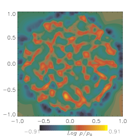
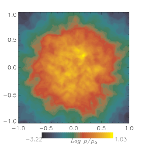
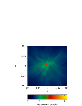
Figure 4: Iso-density plots for model 1.

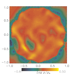
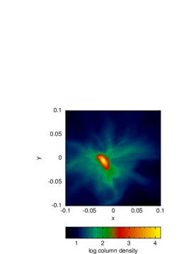
Figure 5: Iso-density plots for model 2.

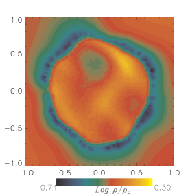
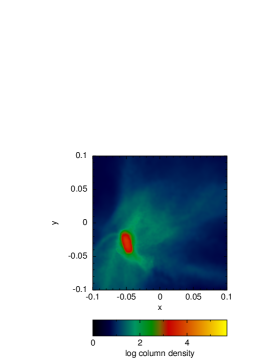
Figure 6: Iso-density plots for model 3.

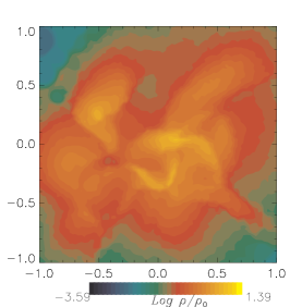
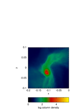
Figure 7: Iso-density plots for model 4.

By looking at the left and middle panels of Figs. 4, 5, 6, and 7, which correspond to models 1, 2, 3, and 4, we note that as the wavelength of the initial perturbation increases, so do the sizes of the initial over-density clumps, and the number of clumps that form across the core decreases.

Due to the loss of homogeneity in the initial distribution of the over-dense clumps, the protostar in formation accretes mass from the surroundings in an anisotropic manner; as a consequence, the protostar moves slightly from the center, in the south and southwest directions, as can be seen in the right panels of Figs. 6 and 7, which correspond to models 3 and 4.

Fig. 2 shows that for models 1–4, the larger the initial perturbation size, the earlier the local peak in the density curve occurs. Besides, we note that the peak velocity in the collapsing region decreases as the size of the initial perturbation increases; see column 5 of Table 1.

0.3.2 Models 5–8

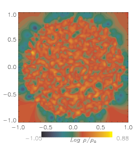
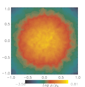
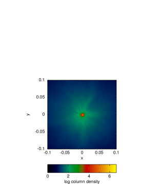
Figure 8: Iso-density plots for model 5.

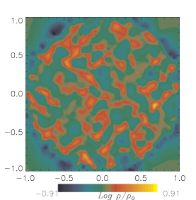
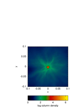
Figure 9: Iso-density plots for model 6.

Here we re-calculate models 1–4, keeping all their parameters unchanged except the number of grid elements of the Fourier mesh; see column 3 of Table 1. We first note that the number of small over-density clumps formed at the initial snapshots increases, but they are still homogeneously distributed across the core volume; see the left panels of Figs. 8 and 9 and compare them with those of models 2–3.

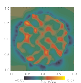
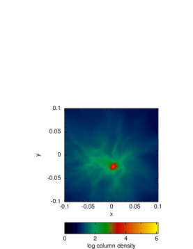
Figure 10: Iso-density plots for model 7.

The loss of homogeneity in the initial distribution of over-density clumps is noticeable in model 7, as can be seen in Fig. 10. A significant reduction in the number of the initial over-density clumps can also be seen in the initial snapshot of model 8; see the left panel of Fig. 10. However, by comparing this panel with that of model 4, shown in Fig. 7, we see that there are a very few more over-density clumps than those formed in model 4.

0.3.3 Models 9–11

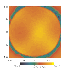
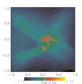
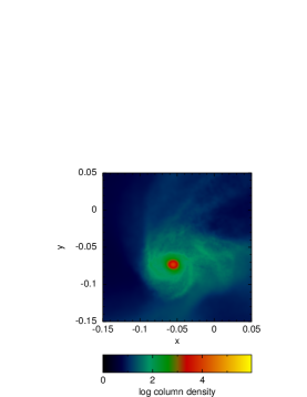
Figure 12: Iso-density plots for model 9.

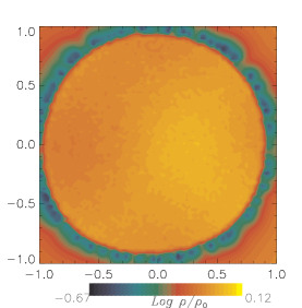
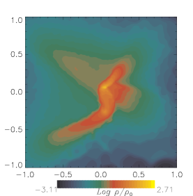
Figure 13: Iso-density plots for model 10.

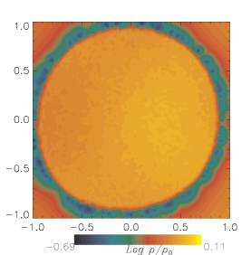
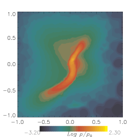
Figure 14: Iso-density plots for model 11.

In these models, the wavelength of the initial perturbation far exceeds the core radius; see column 2 of Table 1. It can be seen in the left panel of Fig. 12 that only two over-density clumps are clearly visible in the equatorial slice of model 9. These perturbations are coupled to deform the central core simultaneously in two orthogonal directions, see the panel in the middle of Fig. 12. By looking at the right panel of Fig. 12, we see the appearance of small spiral arms around the protostar, indicating that the protostar has gained a net angular momentum as a consequence of the small number of coupled perturbations that acted upon it initially. For model 10, we see that only one over-density is visible at the initial snapshot shown in the left panel of Fig. 13. For this reason, the still forming protostar can be seen to be highly deformed, mainly along a single direction; see the left and middle panels of Fig. 13. Thus, the right panel of Fig. 13 shows that the still forming protostar drags a long tail of gas along this single direction. The same behavior is mainly observed for model 11; see Fig. 14.

0.3.4 Models 12–14

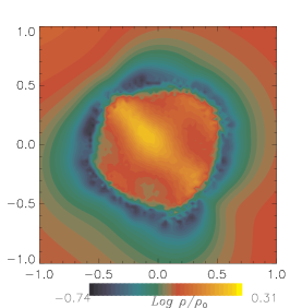
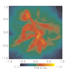
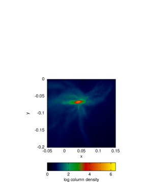
Figure 15: Iso-density plots for model 12.

For these models we use more Fourier modes to re-calculate the models of Section 0.3.3. Let us examine model 12 shown in Fig. 15 and compare it with model 9 shown in Fig. 12. We first note that there is only one perturbation mode visible in the left panel of Fig. 15; despite this, there are a few dominant directions along which the initial over-density grows; see the middle panel of Fig. 15. The velocity of the collapsing peak is significantly greater in model 12 than that observed in model 9; see column 5 of Table 1. Because of this, it is very likely that the protostar formed in model 12 has gained a net angular momentum higher than that of the protostar of model 9, as is suggested by looking at the right panel of Fig. 15.

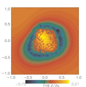
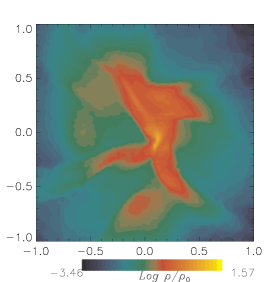
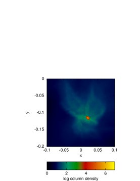
Figure 16: Iso-density plots for model 13.

The size of the initial over-density clump induced by the perturbation mode of model 13 looks smaller than that induced in model 10; compare Fig. 16 with Fig. 13.

In model 14 we observe the occurrence of fragmentation of the central core region, so that a binary protostar system is formed.

0.3.5 Models 15–18

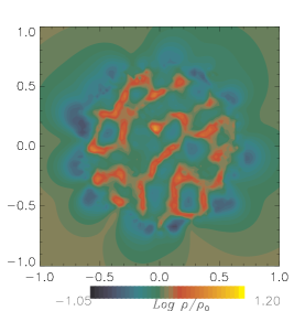
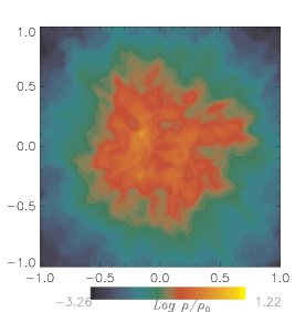
Figure 18: Iso-density plots for model 15.

We consider now the set of models generated with the curl-free turbulence spectrum. In the left panel of Fig. 18, we see that the number of over-density clumps formed initially in model 15 is smaller than the number observed in model 1, shown in the left panel of Fig. 4. The clumps seen in Fig. 18 are also in fact larger that those seen in Fig. 4. Despite this, we still see that the curl-free turbulence spectrum creates a homogeneous distribution of over-density clumps. At the time 0.67 t_ff, when the strong collapse is yet to begin, the spherical symmetry of the collapsing core is already visible in the middle panel of Fig. 18. For this reason, we see that the resulting protostar accretes gas from the remaining core almost isotropically; see the right panel of Fig. 18.

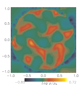
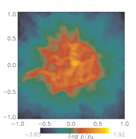
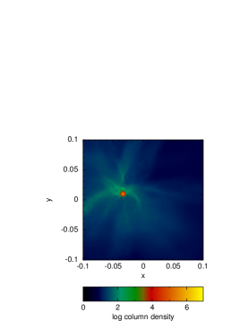
Figure 19: Iso-density plots for model 16.

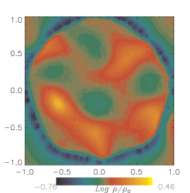
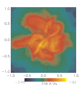
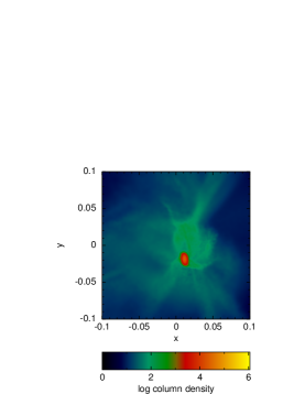
Figure 20: Iso-density plots for model 17.

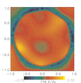
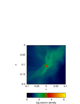
Figure 21: Iso-density plots for model 18.

When the size of the Fourier mesh begins to increase in terms of the core radius, which is shown in models 16–18, then the initial over-density clumps are formed thicker and their number is smaller than those seen in model 15; see the left panels of Figs. 19, 20 and 21. As a consequence, the homogeneity and isotropy of the over-density clump distribution is slightly lessened, and then some clumps grow forming large filaments, as can be observed in the right panels of Figs. 20 and 21. All these models finish with a single protostar formed in the collapsed central region.

By comparing the left panels of Figs. 19, 20 and 21, corresponding to models 16–18, with those of models 2–4, shown in Fig. 5, 6 and 7, we conclude that when the Fourier mesh begins to increase, the models generated with a divergence-free turbulence lose the homogeneity and isotropy of the initial over-density clump distribution earlier than those models generated with a curl-free turbulence.

0.3.6 Models 19–22

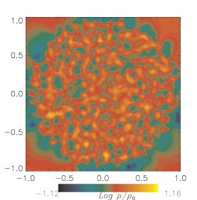
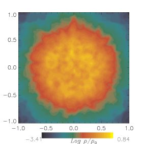
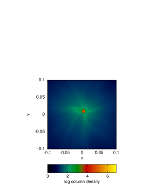
Figure 22: Iso-density plots for model 19.

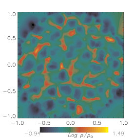
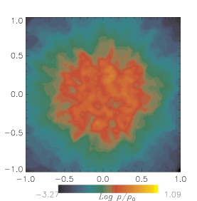
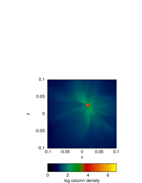
Figure 23: Iso-density plots for model 20.

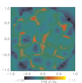
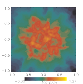
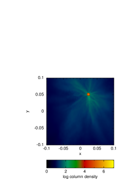
Figure 24: Iso-density plots for model 21.

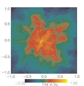
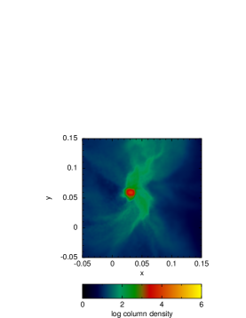
Figure 25: Iso-density plots for model 22.

When the number of Fourier modes increases, then the number of over-density clumps induced initially also increases, so that an homogeneous distribution of small length over-density clumps is formed; see the left panel of Fig. 22 and compare it with the left panel of Fig. 18. When the size of the Fourier mesh increases, which is the case of models 20–22, then we observe the formation of a smaller number of over-density clumps; see the left panels Figs. 23 and 24 and compare them with those of Figs. 19 and 20. However, for model 22, the length of the over-density clumps begins also to increase; see the left panel of Fig. 25 and compare it with that of Fig. 21 of model 18.

We thus conclude that with a larger number of modes, the loss of the homogeneity and isotropy of the initial over-density clump distribution is more delayed; see the left panels of Figs. 23, 24, and 25.

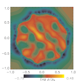
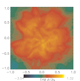
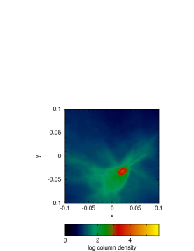
Figure 11: Iso-density plots for model 8.

We do not see any significant difference between the initial panels of models 19–20 shown in Figs. 22–23 and those of models 5–6 shown in Figs. 8–9, so that the two types of turbulence spectra are almost indistinguishable. However, by comparing the initial over-density distribution of clumps for models 21 and 22, shown in Figs. 24 and 25, with those of models 7 and 8, shown in Figs. 10 and 11, we see that the over-density clumps are in general larger for the divergence-free turbulence type than those generated with the curl-free turbulence type.

0.3.7 Models 23–25

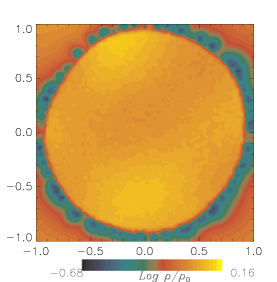
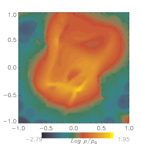
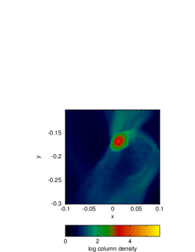
Figure 26: Iso-density plots for model 23.

When the size of the perturbation mode increases further, as for models 23–25, then it is evident the there are only two main directions along which the initial over-density clump distributions grow: see the left panels of Fig. 26, 27 and 28. For this reason, the deformation in the core shape is very significant; see the right panels of Fig. 26, 27 and 28. Despite this, the final outcome of these models is still a single protostar, which is displaced away from the central region, as a consequence of the highly anisotropic accretion of gas.

By comparing the initial clump distributions of models 23–25 with those of models 9–11, shown in Figs. 12, 13 and 14, we note that the over-density grow in orthogonal directions for these two set of models. This observation is expected according to Eqs. 11 and 15, as the velocities are orthogonal vectors.

0.3.8 Models 26–28

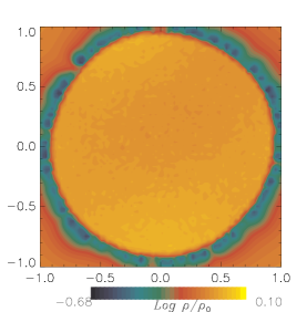
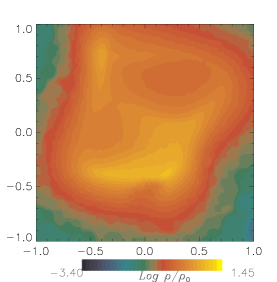
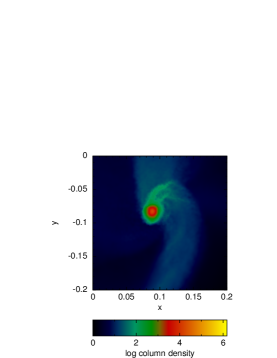
Figure 27: Iso-density plots for model 24.

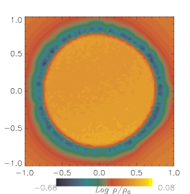
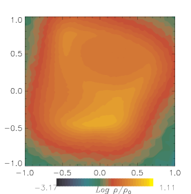
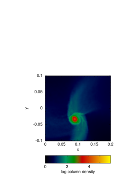
Figure 28: Iso-density plots for model 25.

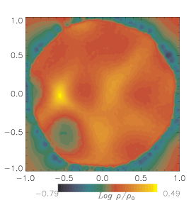
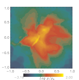
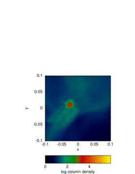
Figure 29: Iso-density and plots for model 26.

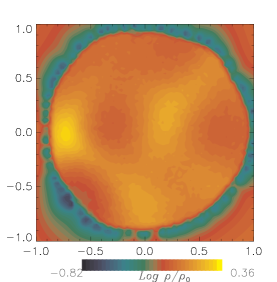
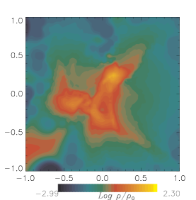
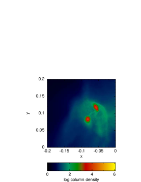
Figure 30: Iso-density plots for model 27.

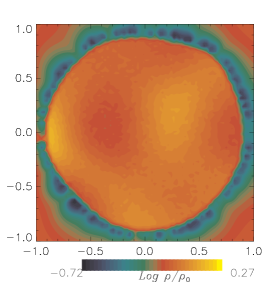
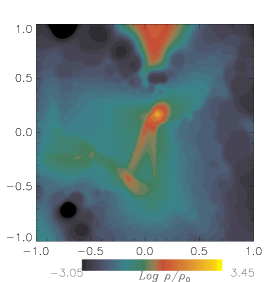
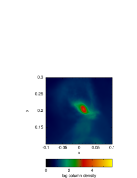
Figure 31: Iso-density plots for model 28.

When the number of Fourier modes increases, as in models 26–27, which are shown in Figs. 29, 30 and 31, in a set of models with a large number of modes, as in models 23–25 shown in Figs. 26, 27 and 28, then we observe that the core is more deformed, so that even core disruption can be achieved, as was the case with model 27, in which a binary protostars system is formed.

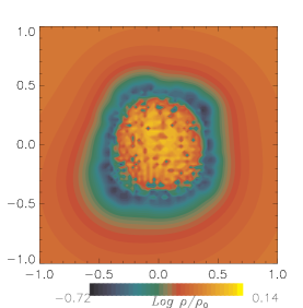
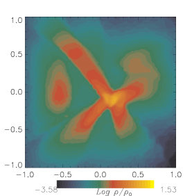
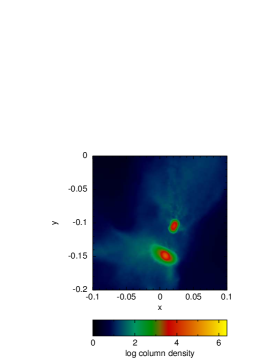
Figure 17: Iso-density plots for model 14.

The same behavior was observed in models 12–14, shown in Figs. 15, 16 and 17, in which we see again the orthogonal directions of the growth of the over-density clumps when compared with those observed in models 26–28.

0.3.9 Integral properties

We present here some integral properties of the resulting protostars, such as the mass and the values of the energy ratios $\alpha_{f}$ and $\beta_{f}$. These properties are calculated by using a subset of the simulation particles, which are determined by means of the following procedure. We first locate the highest density particle in the collapsed central region of the last available snapshot for each model; this particle will be the center of the protostar. We then find all the particles which (i) have density above some minimum value, given by $\log_{10}\left(\rho_{min}/\rho_{0}\right)=1.0$ for all the turbulent models; (ii) are also located within a given maximum radius r_max from the protostar’s center.

All the calculated integral properties are reported in Table 2, whose entries are as follows. The first column shows the number of the model; the second column shows the parameter r_max in terms of the initial core radius R₀; the third column shows the mass of the protostar given in terms of M_⊙; the fourth and fifth columns give the values of $\alpha_{f}$ and $\beta_{f}$, respectively.

There are two lines in Table 2 for models 14 and 27, as their outcomes are binary protostar systems, so that each line indicates the properties of each binary protostar. For these resulting binary systems, we simply define the binary separation as the distance between the centers associated with each protostar. We find the the separation is 163 AU for each binary system.

We find that the average mass of the protostars for models 1–13, excluding model 14, whose outcome is a binary system, is 0.94 M_⊙, with a standard deviation of 0.47 M_⊙. Analogously, the protostar average mass for models 15–26 and 28, excluding the mass of the binary of model 27, is 0.67 M_⊙, with a standard deviation of 0.34 M_⊙. It must be emphasized that these mass relations do not change much if we include the mass of the protostars in the binaries.

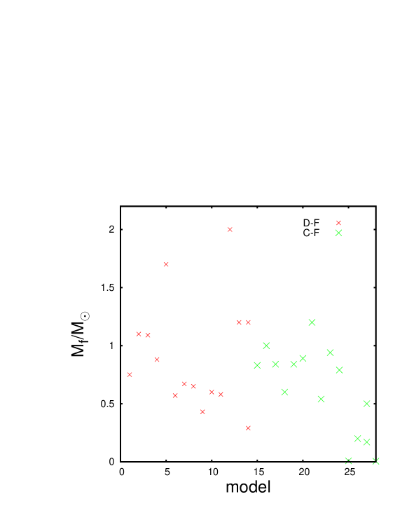
Figure 32: Proto-stellar mass in terms of the simulation model number.

In Fig. 32 we show the mass of the protostars in terms of the simulation model number. It seems that there is nothing that allows us to clearly distinguish the turbulent spectrum used initially; neither is there any trend to assess the effect that the increase in the number of Fourier modes can have on the resulting protostar mass; see also Table 2. However, there seems to be a tendency to low protostar masses for higher model numbers in both turbulence spectra. If this is true, then it would imply that the larger the perturbation mode, the lower the protostar mass.

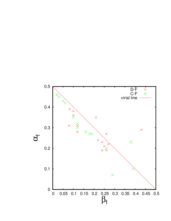
Figure 33: Dimensionless energy ratios of the resulting protostars.

In Fig. 33, we show that most protostars are near or on their way towards virialization, as they are close to the virial line; see Section 0.2.5.It should be noticed that this tendency of collapsing cores to evolve toward the virial line was first pointed out by Boss (1980) and Boss (1981). We also see that higher values of $\alpha_{f}$ and $\beta_{f}$ are obtained for the curl-free turbulence type.

0.4 Discussion

Much similarity of the core collapses is already noticeable by comparing Figs. 2 and 3. In these figures, there is a local density peak in the early evolution stage, which is a consequence of the collisions of particles whose velocities have been assigned randomly by means of a turbulent spectrum with a given number of Fourier modes in a Fourier mesh of a given size. By looking at the third panel of each of these figures, we note that the 64³ modes used in models 9–11 of the divergence-free turbulent type and models 23–25 of the curl-free turbulent type are equally insufficient to capture these local density peak.

The fact that these local peaks are of the same order irrespective of the turbulence type indicates that the initial density fluctuations are also of the same order. Despite this, we find that the average protostar mass of the divergence-free turbulent models is larger than of the curl-free turbulent models; see Section 0.3.9.

With regard to the peak velocity of the collapsing core’s central region, we find a significant similarity between the two turbulence types: the average collapsing velocity is 7.75 km/s for the divergence-free type and 7.6 km/s for the curl-free type. However, the interval of velocities of the former type of turbulence is in general wider than that of the latter type of turbulence.

Another very important issue to discuss is the low level of fragmentation observed in the suite of turbulent models. A first consideration is that we do not use the sink technique introduced by Bate et al. (1995), so that the simulations presented here do not evolve further in time than t_ff. If we were able to follow the simulations longer, we would possibly see the fragmentation of the spiral arms seen surrounding some protostars or the fragmentation of the highly deformed over-density clumps seen in models with a large number of perturbation modes.

A second consideration was already mentioned in Section 0.2.1, that the core considered in this paper was very dense and with a significant thermal support; see also Section 0.2.5. For these two reasons, we expect that the turbulence spectra induced initially find it more difficult to compress the gas randomly across the core. The density of the core in our simulations is ten times larger than the central core considered by Goodwin et al. (2004a), Goodwin et al. (2004b), Goodwin et al. (2006); see also Attwood et al. (2009). We suppose that fragmentation can be prevented in a central core of higher density.

A third consideration is the stochastic nature of the turbulent spectra. In this paper we fixed the seed to generate random numbers, so that all the simulations ran using the same seed. In other papers, it has been shown that different random realizations of the same simulation can have significant differences in their outcomes; see for instance Walch et al. (2009), who used four random seeds in their simulations.

A fourth consideration is that the turbulent velocity fluctuations considered in this paper provide the core with a net angular momentum; see Section 0.2.6 and Fig. 1. We calculated the specific angular momentum with respect to the origin of coordinates (shown in Fig. 1 ) and with respect to each of the X, Y and Z axes, as well. We did not observe any significant difference in these angular momentum calculations, but only small changes due to random velocity fluctuations in a frame with spherical symmetry.

Let us now mention that for rotating cores, $\beta$, defined in Section 0.2.5, would correspond to the ratio of rotational energy to gravitational energy, and a value of 0.21 (see Eq.19) can be considered high with respect to observational values, because their specific angular momentum varies within a range 1 $\times 10^{20}$-2 $\times 10^{22}$ ; see Goodman et al. (1993); Bodenheimer (1995). For this reason, fragmentation can be easily obtained from the collapse of this kind of rotating cores; see Arreaga and Saucedo (2012) and Arreaga (2016). As we mentioned in Section 0.2.6, the level of angular momentum initially given to our models is low compared to typical values of rotating cores and this is the key to understand why we observed only two models with binary formation.

The protostar masses in the divergence-free turbulence models are in the range 0.29–2 M_⊙ while for the curl-free models the masses vary within 0.2–1.2 M_⊙. These masses are in any case much too much larger than those obtained from the collapse of a rotating uniform core of similar total mass and initial energy ratios; see for instance Arreaga (2016) and Arreaga (2017), where the masses generally obtained by numerical simulations of binary formation are around $0.01\,M_{\odot}$. Goodwin et al. (2004a) obtained a wide distribution of protostar masses, with a peak around 1 M_⊙. Large masses, like the ones obtained from turbulent models, are therefore in better agreement with recent VLA and CARMA observations, which showed that the proto-stellar masses of systems such as CB230 IRS1 and L1165-SMM1 have been detected in the range of $0.1-0.25\,M_{\odot}$; see Tobin at al. (2013).

The binary systems obtained in this paper have a mass ratio of q₁₄=0.24 and q₂₇=0.34 for models 14 and 27, respectively. Goodwin et al. (2004a) obtained a $q$ distribution for wide binaries in the range 0.1–0.7 with a peak in the range 0.6–0.7; however, as the binaries evolved, the peak of the $q$ distributions moved to smaller values. In any case, our $q$ values are in agreement with Goodwin et al. (2004a).

0.5 Concluding Remarks

In this paper we considered the gravitational collapse of a uniform core, in which only two types of turbulent velocity spectra have been initially implemented.

It must be emphasized to all the simulations satisfy the same energy requirements, contained in the ratios $\alpha$ and $\beta$; see Eq. 19 of Section 0.2.5. Therefore, it is because of this last statement that we observe a lot similarity in the outcomes of the models, irrespective of the turbulence type considered.

Besides, as we mentioned at the end of Section 0.2.5, the models do not have different levels of turbulence, as the ratio of the turbulent energy to the gravitational energy was fixed at $\gamma_{turb}=0.11$ for all the simulations. It should also be noted that the differences observed between the models can not be attributed to a different random realization of a given simulation, as the random seed used to generate each model was fixed at the same value for all the simulations.

For these reasons, we consider that we achieved the main objective of this paper, so that the different outcomes in the models are due to the change in the number and size of the Fourier modes of the two types of velocity spectra considered. By comparing the plots shown in Section 0.3, we are able to summarize the following observations:

1. The larger the wave length of the perturbation mode, the longer the collapse; in fact, for the models with the largest wavelength modes, we observed a collapse delay up to 0.2 $t_{ff}$ with respect to the models with the shortest wavelength modes.

2. We observe that a larger wave length of the initial perturbation lengthens the initial over-dense clumps, softens the density contrast, and decreases the velocity of the particles in the region of collapse.

3. When the Fourier mesh size begins to increase in terms of the core radius, then the divergence-free turbulence type loses the homogeneity and isotropy of the initial over-density clump distribution earlier than does the curl-free turbulence.

4. The initial appearance of elongated clumps is delayed by increasing the number of Fourier modes.

5. Fragmentation can be induced by increasing the number of perturbation modes.

6. The resulting protostars of all the models with very large perturbation modes have a net angular momentum, which is also a consequence of the highly anisotropic accretion of gas.

7. The protostars obtained from divergence-free turbulence are more massive, in general, than those from models with a curl-free turbulence.

8. In particular, the binary protostar system formed from divergence-free turbulence is also more massive than that formed from the curl-free turbulence.

9. The larger the perturbation mode, the lower the resulting protostar mass.

10. The protostar masses in turbulent models are larger than those obtained from the collapse of a rotating uniform core of similar total mass and initial energy.

    However, due to the stochastic nature of the turbulent spectra, these observations must be validated by more simulations; therefore it is necessary to perform a larger ensemble of simulations to have a statistically representative sample of results, which hopefully can help to validate our observations.

Table 1: Turbulent models and their resulting configurations

Model	$C_{R}$	$N_{x}=N_{y}=N_{z}$	${\cal M}_{max}$	vmax [km/s]	Figure	Turbulence Type	Configuration
1	1	64	4.5	8.1	4	D-F	S
2	2	64	4.48	7.8	5	D-F	S
3	3	64	4.49	7.2	6	D-F	S
4	4	64	4.48	6.3	7	D-F	S
5	1	128	5.09	7.9	8	D-F	S
6	2	128	4.84	7.1	9	D-F	S
7	3	128	4.78	6.8	10	D-F	S
8	4	128	4.6	5.9	11	D-F	S
9	6	64	3.5	5.7	12	D-F	S
10	8	64	3.5	7.0	13	D-F	S
11	10	64	3.25	7.0	14	D-F	S
12	6	128	3.9	11.1	15	D-F	S
13	8	128	3.97	10.9	16	D-F	S
14	10	128	4.04	9.7	17	D-F	B
15	1	64	5.09	8.6	18	C-F	S
16	2	64	4.19	9.5	19	C-F	S
17	3	64	3.99	7.4	20	C-F	S
18	4	64	3.82	6.6	21	C-F	S
19	1	128	4.73	9.5	22	C-F	S
20	2	128	4.9	9.2	23	C-F	S
21	3	128	5.02	10.5	24	C-F	S
22	4	128	4.3	5.7	25	C-F	S
23	6	64	3.5	6.6	26	C-F	S
24	8	64	3.0	7.4	27	C-F	S
25	10	64	2.7	6.4	28	C-F	S
26	6	128	4.11	5.9	29	C-F	S
27	8	128	4.03	7.1	30	C-F	B
28	10	128	3.43	6.0	31	C-F	S

Table 2: Physical properties of protostars

Model	rmax/R0	Mf/M⊙	$\left|\alpha_{f}\right|$	$\left|\beta_{f}\right|$
1	0.008	0.75	0.36	0.10
2	0.01	1.1	0.21	0.25
3	0.017	1.09	0.19	0.26
4	0.01	0.88	0.19	0.24
5	0.005	1.7	0.35	0.21
6	0.005	0.57	0.39	0.082
7	0.008	0.67	0.27	0.26
8	0.01	0.65	0.23	0.24
9	0.007	0.43	0.31	0.079
10	0.008	0.6	0.28	0.12
11	0.007	0.58	0.31	0.12
12	0.013	2.0	0.22	0.27
13	0.004	1.2	0.38	0.1
14	0.0095	1.2	0.24	0.22
14	0.005	0.29	0.29	0.43
15	0.005	0.83	0.42	0.06
16	0.005	1.0	0.46	0.02
17	0.01	0.84	0.27	0.18
18	0.007	0.6	0.35	0.1
19	0.004	0.84	0.46	0.02
20	0.005	0.89	0.43	0.05
21	0.005	1.2	0.45	0.03
22	0.0095	0.54	0.28	0.16
23	0.016	0.94	0.2	0.26
24	0.0095	0.79	0.27	0.19
25	0.01	0.008	0.07	0.29
26	0.0095	0.2	0.32	0.12
27	0.008	0.5	0.3	0.12
27	0.007	0.17	0.23	0.38
28	0.015	0.005	0.10	0.39

Figure 1: The initial specific angular momentum $L/M_{0}$ against the model number. The horizontal lines indicate the observed values of $L/M_{0}$ for real cores; see  Goodman et al. (1993); Bodenheimer (1995).

Figure 2: Time evolution of the peak density $\rho_{max}$ of the divergence-free turbulence models.

Figure 3: Time evolution of the peak density $\rho_{max}$ of the curl-free turbulence models.

References

- André (2007) André P., Belloche, A., Motte, F. and Peretto, N., 2007, Astron. Astrophys. 472, 519.
- Arreaga et al. (2009) Arreaga, G., Klapp, J. and Gomez, F., 2009, Astron. Astrophys. 509, p. A96.
- Arreaga and Saucedo (2012) Arreaga-García, G. and Saucedo-Morales, J.C., 2012, Revista Mexicana de Astronomía y Astrofísica 48, pp. 61–84.
- Arreaga (2016) Arreaga-García, G., 2016, Revista Mexicana de Astronomía y Astrofísica 52, pp. 155–169.
- Arreaga (2017) Arreaga-García, G., 2017, Astrophysics and Space Science 362, pp. 47.
- Arreaga and Klapp (2014) Arreaga-García, G. and Klapp, J., 2014, in: Computational and Experimental Fluid Mechanics with Applications to Physics, Engineering and the Enviroment, Editors: L. Sigalotti, J. Klapp and E. Sira. Springer-Verlag, pp. 509–520.
- Attwood et al. (2009) Attwood, R.E., Goodwin, S.P., Stamatellos, D. and Whitworth, A.P., 2009, Astron. Astrophys. 495, pp. 201–215.
- Ballesteros et al. (1999) Ballesteros-Paredes, J., Hartmann, L. and Vazquez-Semanedi, E., 1999, ApJ527, pp. 285.
- Balsara (1995) Balsara, D., 1995, J. Comput. Phys. 121, 357.
- Bate et al. (1995) Bate, M.R., Bonnell, I.A. and Price, N.M., 1995, MNRAS277, pp. 362–376.
- Bate and Burkert (1997) Bate, M.R. and Burkert, A., 1997, MNRAS288, 1060.
- Bergin et al. (2007) Bergin, E. and Tafalla, M., 2007, Annu. Rev. Astro. Astrophys. 45, 339.
- Bodenheimer (1995) Bodenheimer, P., 1995, ARA&A, 33, 199.
- Bonazzola (1987) Bonazzola, S., Falgorone, E., Heyvaerts, J., Pérault, M., Puget, J.L., 1987, Astron. Astrophys. 172, 293.
- Boss and Bodenheimer (1979) Boss, A.P. and Bodenheimer, P. 1979, ApJ234, 289.
- Boss (1980) Boss, A.P. , 1980, ApJ242, 699-709.
- Boss (1981) Boss, A.P. , 1981, ApJ250, 636644.
- Brunt et al. (2009) Brunt, C.M., Heyer, M.H. and Mac Low, M.M., 2009, Astron. Astrophys. 504, 883.
- Bouwman (2004) Bouwman, A.P., 2004, Astrophysics and Space Science 292, 325.
- Boss et al. (2000) Boss, A.P., Fisher, R.T., Klein, R. and McKee, C.F., 2000, ApJ528, 325.
- Burkert and Bodenheimer (1993) Burkert, A. and Bodenheimer, P., 1993, MNRAS264, 798.
- Caselli et al. (2002) Caselli, P., Benson, P.J., Myers, P.C. and Tafalla, M., 2002, ApJ572, 238.
- Chandrasekhar (1951) Chandrasekhar, S., 1951, Proc. R. Soc. London 210, 26.
- Dobbs et al. (2005) Dobbs, C.L., Bonnell, I.A. and Clark, P.C., 2005, MNRAS360, pp. 2–8.
- Elmegreen (1993) Elmegreen, B.G., 1993, in: Protostars and Planets III, pp. 97.
- Federrath et al. (2010) Federrath, C., Roman-Duval, J., Klessen, R.S., Schmidt, W. and Mac Low, M.M., 2010, Astron. Astrophys. 512, A81.
- Goodman et al. (1993) Goodman, A.A., Benson, P.J., Fuller, G.A., Myers, P.C., 1993, ApJ, 406, pp.528-547.
- Goodwin et al. (2004a) Goodwin, S.P., Whithworth, A.P. and Ward-Thompson, D., 2004, Astron. Astrophys. 414, pp. 633–650.
- Goodwin et al. (2004b) Goodwin, S.P., Whithworth, A.P. and Ward-Thompson, D., 2004, Astron. Astrophys. 423, pp. 169.
- Goodwin et al. (2006) Goodwin, S.P., Whithworth, A.P. and Ward-Thompson, D., 2006, Astron. Astrophys. 452, pp. 487.
- Hachisu and Heriguchi (1984) Hachisu, I. and Heriguchi, Y., 1984, Astron. Astrophys. 140, 259.
- Hachisu and Heriguchi (1985) Hachisu, I. and Heriguchi, Y., 1985, Astron. Astrophys. 143, 355.
- Léorat (1990) Léorat, J., Passot, T. and Pouquet, A., 1990, MNRAS243, 293–311.
- Myers (2005) Myers, P.C., 2005, ApJ623, 280.
- Miyama et al. (1984) Miyama, S.M., Hayashi, C. and Narita, S., 1984, ApJ279, 621.
- Monaghan and Gingold (1983) Monaghan, J.J. and Gingold, R.A., 1983, J. Comput. Phys. 52, 374.
- Press et al. (1992) Press, W.H., Teukolsky, S.A., Vetterling, W.T. and Flannery, B.P., 1992, Numerical Recipes in Fortran 77, Second Edition, Cambridge University Press.
- Padoan et al. (2014) Padoan, P., Federrath, C., Chabrier, G., Evans II, N.J., Johnstone, D., Jrgensen, J.K., McKee, C.F. and Nordlund, E., 2014, Protostars and Planets VI, Henrik Beuther, Ralf S. Klessen, Cornelis P. Dullemond, and Thomas Henning (eds.), University of Arizona Press, Tucson, 914 pp., p.77-100. arXiv. 1312.5365.
- Sigalotti and Klapp (2001) Sigalotti, L. and Klapp, J., 2001, Int. J. Mod. Phys. D 10, 115.
- Sasao (1973) Sasao, T., 1973, PASJ 25, 1.
- Springel (2005) Springel, V., 2005, MNRAS364, 1105.
- Springel et al. (2001) Springel, V., Yoshida, N. and White, S.D.M., 2001, New Astronomy 6, 79.
- Tafalla et al. (1998) Tafalla, M., Mardones, D. and Myers, P.C., 1998, ApJ504 pp. 900–914.
- Tafalla et al. (2004) M. Tafalla, M., Myers, P.C., Caselli, P. and Walmsley, C.M., 2004, Astron. Astrophys. 416, pp. 191–212.
- Tobin at al. (2013) Tobin, J.J., Chandler, C., Wilner, D.J., Looney, L.W., Loinard, L., Chiang, H.-F., Hartmann, L., Calvet, N., D’Alessio, P., Bourke, T.L. and Kwon, W., 2013, ApJ779.
- Tohline (2002) Tohline, J.E., 2002, ARA&A 40, 349.
- Truelove et al. (1997) Truelove, J.K., Klein, R.I., McKee, C.F., Holliman, J.H., Howell, L.H. and Greenough, J.A., 1997, ApJ489, L179.
- Tsuribe et al. (1999) Tsuribe, T. and Inutsuka, S.-I., 1999, ApJ523, pp. L155–L158. Tsuribe, T. and Inutsuka, S.-I., 1999, ApJ526, pp. 307–313.
- Walch et al. (2009) Walch, S., Whitworth, A.P. and Girichidis, P., 2009, MNRAS419, pp. 760–770.
- Whitehouse and Bate (2006) Whitehouse, S.C. and Bate, M.R., 2006, MNRAS367, 32.
- Whithworth and Ward-Thompson (2001) Whithworth, A.P. and Ward-Thompson, D., 2001, ApJ54, 317.