IFT-UAM/CSIC-17-050

FTUAM-17-10

Non-perturbative renormalization of tensor currents:

strategy and results for $N_{f}=0$ and $N_{f}=2$ QCD

C. Pena^a,b, D. Preti^b

^a Departamento de Física Teórica, Universidad Autónoma de Madrid

Cantoblanco E-28049 Madrid, Spain

^b Instituto de Física Teórica UAM-CSIC

c/ Nicolás Cabrera 13-15, Universidad Autónoma de Madrid

Cantoblanco E-28049 Madrid, Spain

Abstract: Tensor currents are the only quark bilinear operators lacking a non-perturbative determination of their renormalisation group (RG) running between hadronic and electroweak scales. We develop the setup to carry out the computation in lattice QCD via standard recursive finite-size scaling techniques, and provide results for the RG running of tensor currents in $N_{f}=0$ and $N_{f}=2$ QCD in the continuum for various Schrödinger Functional schemes. The matching factors between bare and renormalisation group invariant currents are also determined for a range of values of the lattice spacing relevant for large-volume simulations, thus enabling a fully non-perturbative renormalization of physical amplitudes mediated by tensor currents.

1 Introduction

Hadronic matrix elements of tensor currents play an important rôle in several relevant problems in particle physics. Some prominent examples are rare heavy meson decays that allow to probe the consistency of the Standard Model (SM) flavour sector (see, e.g., [1, 2, 3] for an overview), or precision measurements of $\beta$-decay and limits on the neutron electric dipole moment (see, e.g., [4, 5, 6] for an up-to-date lattice-QCD perspective).

One of the key ingredients in these computations is the renormalization of the current. Indeed, partial current conservation ensures that non-singlet vector and axial currents require at worst finite normalizations, and fixes the anomalous dimension of scalar and pseudoscalar densities to be minus the quark mass anomalous dimension. They however do not constrain the tensor current, which runs with the only other independent anomalous dimension among quark bilinears. Controlling the current renormalization and running at the non-perturbative level, in the same fashion achieved for quark masses [7, 8, 9, 10], is therefore necessary in order to control systematic uncertainties, and allow for solid conclusions in new physics searches.

The anomalous dimension of tensor currents is known to three-loop order in continuum schemes [11, 12], while on the lattice perturbative studies have been carried out to two-loop order [13]. Non-perturbative determinations of renormalization constants in RI/MOM schemes, for the typical few-${\rm GeV}$ values of the renormalization scale accessible to the latter, have been obtained for various numbers of dynamical flavours and lattice actions [14, 15, 16, 17, 18, 19, 20]. The purpose of this work is to set up the strategy for the application of finite-size scaling techniques based on the Schrödinger Functional (SF) [21], in order to obtain a fully non-perturbative determination of both current renormalization constants at hadronic energy scales, and the running of renormalized currents to the electroweak scale. This completes the ALPHA Collaboration non-perturbative renormalization programme for non-singlet quark field bilinears [7, 8, 9, 10, 22, 23, 24] and four-quark operators [25, 26, 27, 28, 29, 30, 31].

As part of the strategy, we will set up a family of SF renormalization schemes, and perform a perturbative study with the main purpose of computing the perturbative anomalous dimension up to two loops, in order to make safe contact with perturbative physics at the electroweak scale. Preliminary results of this work have already appeared as proceedings contributions [32]. We will then apply our formalism to the fully non-perturbative renormalization of non-singlet tensor currents in $N_{\mathrm{\scriptstyle f}}=0$ and $N_{\mathrm{\scriptstyle f}}=2$ QCD. Our results for $N_{\mathrm{\scriptstyle f}}=3$ QCD, that build on the non-perturbative determination of the running coupling [34, 35, 36] and the renormalization of quark masses [9, 10, 22], will be provided in a separate publication [37].

The layout of this paper is as follows. In section 2 we will introduce our notation and discuss the relevant renormalization group equations. In section 3 we will introduce our SF schemes, generalizing the ones employed for quark mass renormalization. In section 4 we will study these schemes in one-loop perturbation theory, and compute the matching factors that allow to determine the NLO values of anomalous dimensions. In section 5 we will discuss our non-perturbative computations, and provide results for the running of the currents between hadronic and high-energy scales and for the renormalization constants needed to match bare hadronic observables at low energies. Section 6 contains our conclusions. Some technical material, as well as several tables and figures, are gathered in appendices.

2 Renormalization Group

Theory parameters and operators are renormalized at the renormalization scale $\mu$. The scale dependence of these quantities is given by their Renormalization Group (RG) evolution. The Callan-Symanzik equations satisfied by the gauge coupling and quark masses are of the form

$$\mu\frac{\partial\kern 1.0pt\overline{\kern-1.0ptg\kern 0.0pt}\kern 1.0pt}{\partial\mu} \,=\,\beta(\kern 1.0pt\overline{\kern-1.0ptg\kern 0.0pt}\kern 1.0pt(\mu))\,,$$ (2.1)

$$\mu\frac{\partial\kern 2.0pt\overline{\kern-1.0ptm\kern-1.0pt}\kern 1.0pt_{i}}{\partial\mu} \,=\,\tau(\kern 1.0pt\overline{\kern-1.0ptg\kern 0.0pt}\kern 1.0pt(\mu))\kern 2.0pt\overline{\kern-1.0ptm\kern-1.0pt}\kern 1.0pt_{i}(\mu)\,,$$ (2.2)

respectively, with renormalized coupling $\kern 1.0pt\overline{\kern-1.0ptg\kern 0.0pt}\kern 1.0pt$ and masses $\kern 2.0pt\overline{\kern-1.0ptm\kern-1.0pt}\kern 1.0pt_{i}$; the index $i$ runs over flavour. The renormalization group equations (RGEs) for composite operators have the same form as Eq. (2.2), with the anomalous dimensions of the operators $\gamma$ in the place of $\tau$. Starting from the RGE for correlation functions, we can write the renormalization group equation for the insertion of a multiplicatively renormalizable local composite operator $O$ in an on-shell correlation function as:

$$\mu\frac{\partial\kern 3.0pt\overline{\kern-2.0ptO\kern 0.0pt}\kern 1.0pt(\mu)}{\partial\mu}\,=\,\gamma(\kern 1.0pt\overline{\kern-1.0ptg\kern 0.0pt}\kern 1.0pt(\mu))\kern 3.0pt\overline{\kern-2.0ptO\kern 0.0pt}\kern 1.0pt(\mu)\,.$$ (2.3)

where $\kern 3.0pt\overline{\kern-2.0ptO\kern 0.0pt}\kern 1.0pt(\mu)$ is the renormalized operator. The latter is connected to the bare operator insertion $O(g_{0}^{2})$ through

$$\kern 3.0pt\overline{\kern-2.0ptO\kern 0.0pt}\kern 1.0pt(\mu)=\lim_{a\to 0}Z_{O}(g_{0}^{2},a\mu)O(g_{0}^{2})\,.$$ (2.4)

where $g_{0}$ is the bare coupling, $Z_{O}$ is a renormalization constant, and $a$ is some inverse ultraviolet cutoff — the lattice spacing in this work. We assume a mass-independent scheme, such that both the $\beta$-function and the anomalous dimensions $\tau$ and $\gamma$ depend only on the coupling and the number of flavours (other than on the number of colours $N$); examples of such schemes are the ${\overline{\rm MS}}$ scheme of dimensional regularization [38, 39], RI schemes [40], or the SF schemes we will use to determine the running non-perturbatively [21, 41]. The RG functions then admit asymptotic expansions of the form:

$$\beta(g)\ \underset{g\sim 0}{\approx}\ -g^{3}\big{(}b_{0}+b_{1}g^{2}+b_{2}g^{4}+\ldots\big{)}\,,$$ (2.5)

$$\tau(g)\ \underset{g\sim 0}{\approx}\ -g^{2}\big{(}d_{0}+d_{1}g^{2}+d_{2}g^{4}+\ldots\big{)}\,,$$ (2.6)

$$\gamma(g)\ \underset{g\sim 0}{\approx}\ -g^{2}\big{(}\gamma_{0}+\gamma_{1}g^{2}+\gamma_{2}g^{4}+\ldots\big{)}\,.$$ (2.7)

The coefficients $b_{0}$, $b_{1}$ and $d_{0}$, $\gamma_{0}$ are independent of the renormalization scheme chosen. In particular [42, 43, 44, 45, 46, 47, 48]

$$b_{0} =\frac{1}{(4\pi)^{2}}\left(\frac{11}{3}N-\frac{2}{3}N_{\mathrm{\scriptstyle f}}\right)\,,$$ (2.8)

$$b_{1} =\frac{1}{(4\pi)^{4}}\left[\frac{34}{3}N^{2}-\left(\frac{13}{3}N-\frac{1}{N}\right)N_{\mathrm{\scriptstyle f}}\right]\,,$$ (2.9)

and

$$d_{0}=\frac{6C_{\rm F}}{(4\pi)^{2}}\,,$$ (2.10)

with $C_{\rm F}=\frac{N^{2}-1}{2N}$.

The RGEs in Eqs. (2.1–2.3) can be formally solved in terms of the renormalization group invariants (RGIs) $\Lambda_{\rm\scriptscriptstyle QCD}$, $M_{i}$ and $\hat{O}$, respectively, as:

$$\Lambda_{\rm\scriptscriptstyle QCD} \,=\,\mu\,\frac{[b_{0}\kern 1.0pt\overline{\kern-1.0ptg\kern 0.0pt}\kern 1.0pt^{2}(\mu)]^{-b_{1}/2b_{0}^{2}}}{e^{1/2b_{0}\kern 1.0pt\overline{\kern-1.0ptg\kern 0.0pt}\kern 1.0pt^{2}(\mu)}}\,\exp\left\{-\int_{0}^{\kern 1.0pt\overline{\kern-1.0ptg\kern 0.0pt}\kern 1.0pt(\mu)}{\rm d}g\left[\frac{1}{\beta(g)}+\frac{1}{b_{0}g^{3}}-\frac{b_{1}}{b_{0}^{2}g}\right]\right\}\,,$$ (2.11)

$$M_{i} \,=\,\kern 2.0pt\overline{\kern-1.0ptm\kern-1.0pt}\kern 1.0pt_{i}(\mu)\,[2b_{0}\kern 1.0pt\overline{\kern-1.0ptg\kern 0.0pt}\kern 1.0pt^{2}(\mu)]^{-d_{0}/2b_{0}}\,\exp\left\{-\int_{0}^{\kern 1.0pt\overline{\kern-1.0ptg\kern 0.0pt}\kern 1.0pt(\mu)}{\rm d}g\left[\frac{\tau(g)}{\beta(g)}-\frac{d_{0}}{b_{0}g}\right]\right\}\,,$$ (2.12)

$$\hat{O} \,=\,\kern 3.0pt\overline{\kern-2.0ptO\kern 0.0pt}\kern 1.0pt(\mu)\,\left[\frac{\kern 1.0pt\overline{\kern-1.0ptg\kern 0.0pt}\kern 1.0pt^{2}(\mu)}{4\pi}\right]^{-\gamma_{0}/2b_{0}}\,\exp\left\{-\int_{0}^{\kern 1.0pt\overline{\kern-1.0ptg\kern 0.0pt}\kern 1.0pt(\mu)}{\rm d}g\,\left[\frac{\gamma(g)}{\beta(g)}-\frac{\gamma_{0}}{b_{0}g}\right]\right\}$$

$$\,\equiv\,\hat{c}(\mu)\kern 3.0pt\overline{\kern-2.0ptO\kern 0.0pt}\kern 1.0pt(\mu)\,.$$ (2.13)

While the value of the $\Lambda_{\rm\scriptscriptstyle QCD}$ parameter depends on the renormalization scheme chosen, $M_{i}$ and $\hat{O}$ are the same for all schemes. In this sense, they can be regarded as meaningful physical quantities, as opposed to their scale-dependent counterparts. The aim of the non-perturbative determination of the RG running of parameters and operators is to connect the RGIs — or, equivalently, the quantity renormalized at a very high energy scale, where perturbation theory applies — to the bare parameters or operator insertions, computed in the hadronic energy regime. In this way the three-orders-of-magnitude leap between the hadronic and weak scales can be bridged without significant uncertainties related to the use of perturbation theory.

In order to describe non-perturbatively the scale dependence of the gauge coupling and composite operators, we will use the step-scaling functions (SSFs) $\sigma$ and $\sigma_{O}$, respectively, defined as

$$-\log(s)=\int_{\sqrt{u}}^{\sqrt{\sigma(u)}}\,\frac{dg^{\prime}}{\beta(g^{\prime})}\,,$$ (2.14)

$$\sigma_{O}(s,u)=\exp\left\{\int_{\sqrt{u}}^{\sqrt{\sigma(u)}}\,\frac{\gamma(g^{\prime})}{\beta(g^{\prime})}dg^{\prime}\right\}\,,$$ (2.15)

or, equivalently,

$$\sigma(s,u) =\left.\kern 1.0pt\overline{\kern-1.0ptg\kern 0.0pt}\kern 1.0pt^{2}(\mu/s)\right|_{u=\kern 1.0pt\overline{\kern-1.0ptg\kern 0.0pt}\kern 1.0pt^{2}(\mu)}\,,$$ (2.16)

$$\sigma_{O}(s,u) =U(\mu/s,\mu)\,,$$ (2.17)

where

$$U(\mu_{2},\mu_{1})=\exp\left\{\int_{\sqrt{\kern 1.0pt\overline{\kern-1.0ptg\kern 0.0pt}\kern 1.0pt^{2}(\mu_{1})}}^{\sqrt{\kern 1.0pt\overline{\kern-1.0ptg\kern 0.0pt}\kern 1.0pt^{2}(\mu_{2})}}\,\frac{\gamma(g^{\prime})}{\beta(g^{\prime})}dg^{\prime}\right\}$$ (2.18)

is the RG evolution operator for the operator at hand, which connects renormalized operators at different scales as $\kern 3.0pt\overline{\kern-2.0ptO\kern 0.0pt}\kern 1.0pt(\mu_{2})=U(\mu_{2},\mu_{1})\kern 3.0pt\overline{\kern-2.0ptO\kern 0.0pt}\kern 1.0pt(\mu_{1})$. The SSFs are thus completely determined by, and contain the same information as, the RG functions $\gamma$ and $\beta$. In particular, $\sigma_{O}(s,u)$ corresponds to the RG evolution operator of $\kern 3.0pt\overline{\kern-2.0ptO\kern 0.0pt}\kern 1.0pt$ between the scales $\mu/s$ and $\mu$; from now on, we will set $s=2$, and drop the parameter $s$ in the dependence. The SSF can be related to renormalization constants via the identity

$$\sigma_{O}(u)=\lim_{a\to 0}\Sigma_{O}(u,a\mu)\,,\qquad\Sigma_{O}(u,a\mu)=\left.\frac{Z_{O}(g_{0}^{2},a\mu/2)}{Z_{O}(g_{0}^{2},a\mu)}\right|_{u=\kern 1.0pt\overline{\kern-1.0ptg\kern 0.0pt}\kern 1.0pt^{2}(\mu)}\,.$$ (2.19)

This will be the expression we will employ in practice to determine $\sigma_{O}$, and hence operator anomalous dimensions, for a broad range of values of the renormalized coupling $u$.

In this work we will focus on the renormalization of tensor currents. The (flavour non-singlet) tensor bilinear is defined as

$$T_{\mu\nu}(x)=i\,\bar{\psi}_{s_{1}}(x)\sigma_{\mu\nu}\psi_{s_{2}}(x)\,,$$ (2.20)

where $\sigma_{\mu\nu}={\scriptstyle{{i\over 2}}}[\gamma_{\mu},\gamma_{\nu}]$, and $s_{1}\neq s_{2}$ are flavour indices. Since all the Lorentz components have the same anomalous dimension, as far as renormalization is concerned it is enough to consider the “electric” operator $T_{0k}$. As already done in the introduction, it is important to observe that the tensor current is the only bilinear operator that evolves under RG transformation in a different way respect to the quark mass — partial conservation of the vector and axial currents protect them from renormalization, and fixes the anomalous dimension of both scalar and pseudoscalar densities to be $-\tau$. The one-loop (universal) coefficient of the tensor anomalous dimension is

$$\gamma_{\rm\scriptscriptstyle T}^{(0)}=\frac{2C_{\rm F}}{(4\pi)^{2}}\,.$$ (2.21)

3 Schrödinger Functional renormalization schemes

The renormalization schemes we will consider are based on the Schrödinger Functional [21], i.e. on the QCD partition function ${\cal Z}=\int{\rm D}[A,\bar{\psi},\psi]e^{-S[A,\bar{\psi},\psi]}$ on a finite Euclidean spacetime of dimensions $L^{3}\times T$ with lattice spacing $a$, where periodic boundary conditions on space (in the case of fermion fields, up a to a global phase $\theta$) and Dirichlet boundary conditions at times $x_{0}=0,T$ are imposed. A detailed discussion of the implementation and notation that we will follow can be found in [52]. We will always consider $L=T$ and trivial gauge boundary fields (i.e. there is no background field induced by the latter). The main advantage of SF schemes is that they allow to compute the scale evolution via finite-size scaling, based on the identification of the renormalization scale with the inverse box size, i.e. $\mu=1/L$.

To define suitable SF renormalization conditions we can follow the same strategy as in [53, 54, 8, 55], which has been applied successfully also to several other composite operators both in QCD [56, 57, 58, 25, 26, 27, 28, 29, 23, 24] and other theories. We first introduce the two-point functions

$$k_{\rm\scriptscriptstyle T}(x_{0})=-\frac{1}{6}\sum_{k=1}^{3}\langle T_{0k}(x)\,{\cal O}[\gamma_{k}]\rangle\,,$$ (3.22)

$$f_{1}=-\frac{1}{2L^{6}}\langle{\cal O}^{\prime}_{s_{2}s_{1}}[\gamma_{5}]{\cal O}_{s_{1}s_{2}}[\gamma_{5}]\rangle\,,$$ (3.23)

and

$$k_{1}=-\frac{1}{6L^{6}}\langle{\cal O}^{\prime}_{s_{2}s_{1}}[\gamma_{k}]{\cal O}_{s_{1}s_{2}}[\gamma_{k}]\rangle\,.$$ (3.24)

where

$${\cal O}[\Gamma]=a^{6}\sum_{\mathbf{x},\mathbf{y}}\bar{\zeta}_{s_{2}}(\mathbf{x})\,\Gamma\,\zeta_{s_{1}}(\mathbf{y})$$ (3.25)

is a source operator built with the $x_{0}=0$ boundary fields $\zeta,\bar{\zeta}$. A sketch of the correlation function in the SF is provided in Fig.3. The renormalization constant $Z_{\rm\scriptscriptstyle T}$ is then defined by

$$Z_{\rm\scriptscriptstyle T}(g_{0},a/L)\frac{k_{\rm\scriptscriptstyle T}(L/2)}{f_{1}^{1/2-\alpha}k_{1}^{\alpha}}=\left.\frac{k_{\rm\scriptscriptstyle T}(L/2)}{f_{1}^{1/2-\alpha}k_{1}^{\alpha}}\right|_{m_{0}=m_{\rm cr},\,g_{0}^{2}=0}\,,$$ (3.26)

where we have already fixed $\mu=1/L$, $m_{0}$ is the bare quark mass, and $m_{\rm cr}$ is the critical mass, needed if Wilson fermions are used in the computation — as will be our case. The factor $f_{1}^{1/2-\alpha}k_{1}^{\alpha}$ cancels the renormalization of the boundary fields contained in ${\cal O}[\Gamma]$, which holds for any value of the parameter $\alpha$; we will restrict ourselves to the choices $\alpha=0,1/2$. The only remaining parameter in Eq. (3.26) is the kinematical variable $\theta$ entering spatial boundary conditions; once its value is specified alongside the one of $\alpha$, the scheme is completely fixed. We will consider the values $\theta=0,0.5,1.0$ in the perturbative study discussed in the next section, and in the non-perturbative computation we will set $\theta=0.5$.

figureSketch of correlation function in the SF: bilinear insertion on the left and boundary-to-boundary on the right.

The condition in Eq. (3.26) involves the correlation function $k_{\rm\scriptscriptstyle T}$, which is not $\mbox{O}(a)$ improved. Therefore, the scaling of the renormalized current towards the continuum limit, given by Eq. (2.4), will be affected by $\mbox{O}(a)$ effects. The latter can be removed by subtracting suitable counterterms, following the standard on-shell $\mbox{O}(a)$ improvement strategy for SF correlation functions [52]. On the lattice, and in the chiral limit, the $\mbox{O}(a)$ improvement pattern of the tensor current reads

$$T_{\mu\nu}^{\rm I}=T_{\mu\nu}+ac_{\rm\scriptscriptstyle T}(g_{0}^{2})(\tilde{\partial}_{\mu}V_{\nu}-\tilde{\partial}_{\nu}V_{\mu})\,,$$ (3.27)

where $\tilde{\partial}$ is the symmetrized lattice derivative and $V_{\mu}=\bar{\psi}_{s_{1}}\gamma_{\mu}\psi_{s_{2}}$ is the vector current. Focusing again only on the electric part, the above formula reduces to

$$T_{0k}^{\rm I}=T_{0k}+ac_{\rm\scriptscriptstyle T}(g_{0}^{2})(\tilde{\partial}_{0}V_{k}-\tilde{\partial}_{k}V_{0})\,,$$ (3.28)

which results in an $\mbox{O}(a)$ improved version of the two-point function $k_{\rm\scriptscriptstyle T}$ of the form

$$k_{\rm\scriptscriptstyle T}^{\rm I}(x_{0})=k_{\rm\scriptscriptstyle T}(x_{0})+c_{\rm\scriptscriptstyle T}(g_{0}^{2})\tilde{\partial}_{0}k_{\rm\scriptscriptstyle V}(x_{0})\,,$$ (3.29)

with

$$k_{\rm\scriptscriptstyle V}(x_{0})=-\frac{1}{6}\sum_{k=1}^{3}\langle V_{k}(x)\,{\cal O}[\gamma_{k}]\rangle\,.$$ (3.30)

Note that the contribution involving the spatial derivative vanishes. Inserting $k_{\rm\scriptscriptstyle T}^{\rm I}$ in Eq. (3.26), and the resulting $Z_{\rm\scriptscriptstyle T}$ in Eq. (2.4) alongside the $\mbox{O}(a)$ improved current, will result in $\mbox{O}(a^{2})$ residual cutoff effects in the value of the SSF $\Sigma_{\rm\scriptscriptstyle T}$ defined in Eq. (2.19), provided the action and $m_{\rm cr}$ are also $\mbox{O}(a)$ improved.

4 Perturbative study

We will now study our renormalization conditions in one-loop perturbation theory. The aim is to obtain the next-to-leading (NLO) anomalous dimension of the tensor current in our SF schemes, necessary for a precise connection to RGI currents, or continuum schemes, at high energies; and compute the leading perturbative contribution to cutoff effects, useful to better control continuum limit extrapolations.

We will expand the relevant quantities in powers of the bare coupling $g_{0}^{2}$ as

$$X=\sum_{n=0}^{\infty}g_{0}^{2}X^{(n)}$$ (4.31)

where $X$ can be any of $Z_{\rm\scriptscriptstyle T}$, $k_{\rm\scriptscriptstyle T}$, $k_{\rm\scriptscriptstyle V}$, $f_{1}$, or $k_{1}$. To $\mathcal{O}(g_{0}^{2})$, Eq. (3.28) can be written as

$$k_{\rm\scriptscriptstyle T}^{\rm I}(x_{0})=k_{\rm\scriptscriptstyle T}^{(0)}(x_{0})+g_{0}^{2}\left[k_{\rm\scriptscriptstyle T}^{(1)}(x_{0})+ac_{\rm\scriptscriptstyle T}^{(1)}\tilde{\partial}_{0}k_{\rm\scriptscriptstyle V}^{(0)}(x_{0})\right]+\mathcal{O}(ag_{0}^{4})\,,$$ (4.32)

with $c_{\rm\scriptscriptstyle T}(g_{0}^{2})=c_{\rm\scriptscriptstyle T}^{(1)}g_{0}^{2}+\mathcal{O}(g_{0}^{4})$. The renormalization constant for the improved tensor correlator $k_{\rm\scriptscriptstyle T}^{\rm I}$ at one-loop is then given by

$$\begin{split}&Z_{\rm\scriptscriptstyle T}^{(1)}(a/L)=\\ &-\Bigg{\{}\frac{1}{k_{\rm\scriptscriptstyle T}^{(0)}(T/2)}\left[k_{\rm\scriptscriptstyle T}^{(1)}(T/2)+\tilde{c}_{\rm t}^{(1)}{k_{\rm\scriptscriptstyle T}}_{\rm;bi}^{(0)}(T/2)+m_{\rm cr}^{(1)}\frac{\partial k_{\rm\scriptscriptstyle T}^{(0)}(T/2)}{\partial m_{0}}+c_{\rm\scriptscriptstyle T}^{(1)}\tilde{\partial}_{0}k_{\rm\scriptscriptstyle V}^{(0)}(T/2)\right]\\ &-\left(\frac{1}{2}-\alpha\right)\frac{1}{f_{1}^{(0)}}\left[f_{1}^{(1)}+\tilde{c}_{\rm t}^{(1)}f_{1;{\rm bi}}^{(0)}+m_{\rm cr}^{(1)}\frac{\partial f_{1}^{(0)}}{\partial m_{0}}\right]\\ &-\alpha\frac{1}{k_{1}^{(0)}}\left[k_{1}^{(1)}+\tilde{c}_{\rm t}^{(1)}k_{1;{\rm bi}}^{(0)}+m_{\rm cr}^{(1)}\frac{\partial k_{1}^{(0)}}{\partial m_{0}}\right]\Bigg{\}}\end{split}$$ (4.33)

where $\tilde{c}_{\rm t}$ is the coefficient of the counterterm that subtracts the $\mbox{O}(a)$ contribution coming from the fermionic action at the boundaries, and $am_{\rm cr}^{(1)}$ is the one-loop value of the critical mass, for which we employ the continuum values of $am_{\rm cr}^{(1)}$ from [26, 60]. The one-loop value of the improvement coefficient $c_{\rm\scriptscriptstyle T}$ has been obtained using SF techniques in [61]. We have repeated the computation of this latter quantity as a crosscheck of our perturbative setup; a summary is provided in Appendix A.

Figure 1: One-loop diagrams for boundary-to-bulk correlators.

Figure 2: One-loop diagrams for boundary-to-boundary correlators.

4.1 Perturbative scheme matching

Any two mass-independent renormalization schemes (indicated by primed and unprimed quantites, respectively) can be related by a finite parameter and operator renormalization of the form

$$\kern 1.0pt\overline{\kern-1.0ptg\kern 0.0pt}\kern 1.0pt^{\prime 2} =\chi_{g}(\kern 1.0pt\overline{\kern-1.0ptg\kern 0.0pt}\kern 1.0pt)\kern 1.0pt\overline{\kern-1.0ptg\kern 0.0pt}\kern 1.0pt^{2},$$ (4.34)

$$\kern 2.0pt\overline{\kern-1.0ptm\kern-1.0pt}\kern 1.0pt^{\prime}_{i} =\chi_{m}(\kern 1.0pt\overline{\kern-1.0ptg\kern 0.0pt}\kern 1.0pt)\kern 2.0pt\overline{\kern-1.0ptm\kern-1.0pt}\kern 1.0pt_{i},\quad i=1,\dots,N_{\mathrm{\scriptstyle f}},$$ (4.35)

$$\kern 3.0pt\overline{\kern-2.0ptO\kern 0.0pt}\kern 1.0pt^{\prime} =\chi_{O}(\kern 1.0pt\overline{\kern-1.0ptg\kern 0.0pt}\kern 1.0pt)\kern 3.0pt\overline{\kern-2.0ptO\kern 0.0pt}\kern 1.0pt\,,$$ (4.36)

where we have assumed $O$ to be multiplicatively renormalizable. The scheme change factors $\chi$ can be expanded perturbatively as

$$\chi(g)\stackrel{{\scriptstyle g\sim 0}}{{\approx}}1+\chi^{(1)}g^{2}+\mathcal{O}(g^{4})\,.$$ (4.37)

Plugging Eqs. (4.34, 4.35, 4.36) into the Callan-Symanzik equations allows to relate a change in a renormalized quantity to the change in the corresponding RG function, viz.

$$\beta^{\prime}(g^{\prime}) =\left[\beta(g)\frac{\partial g^{\prime}}{\partial g}\right]_{g=g(g^{\prime})}\,,$$ (4.38)

$$\tau^{\prime}(g^{\prime}) =\left[\tau(g)+\beta(g)\frac{\partial}{\partial g}\log(\chi_{m}(g))\right]_{g=g(g^{\prime})}\,,$$ (4.39)

$$\gamma^{\prime}(g^{\prime}) =\left[\gamma(g)+\beta(g)\frac{\partial}{\partial g}\log(\chi_{O}(g))\right]_{g=g(g^{\prime})}\,.$$ (4.40)

In particular, expanding Eq. (4.40) to order $g^{2}$ provides a useful relation between the 2-loop coefficient of the anomalous dimension in the two schemes, viz.

$$\gamma^{\prime}_{1}=\gamma_{1}+2b_{0}\chi_{O}^{(1)}-\gamma_{0}\chi_{g}^{(1)}.$$ (4.41)

The one-loop matching coefficient $\chi_{g}^{(1)}$ for the SF coupling was computed in [62, 63],

$$\chi_{g}^{(1)}=2b_{0}\log(L\mu)-\frac{1}{4\pi}(c_{1,0}+c_{1,1}N_{\mathrm{\scriptstyle f}})\,,$$ (4.42)

where the logarithm vanishes with our choice $\mu=1/L$, and for the standard definition of the SF coupling one has

$$c_{1,0}=1.25563(4)\,\quad\quad c_{1,1}=0.039863(2)\,.$$ (4.43)

The other finite term $\chi_{O}$ in Eq. (4.40) will provide the operator matching between the lattice-regulated SF scheme and some reference scheme where the NLO anomalous dimension is known, such as ${\overline{\rm MS}}$ or RI, that we will label as “cont”. The latter usually are based on variants of the dimensional regularization procedure; our SF schemes will be, on the other hand, regulated by a lattice. The practical application of Eq. (4.41) thus involves a two-step procedure, in which the lattice-regulated SF scheme is first matched to a lattice-regulated continuum scheme, that is in turned matched to the dimensionally-regulated continuum scheme. This yields

$$[\chi_{O}^{(1)}]_{\rm SF;cont}=[\chi_{O}^{(1)}]_{\rm SF;lat}-[\chi_{O}^{(1)}]_{\rm cont;lat}\,.$$ (4.44)

The one-loop matching coefficients $[\chi_{O}^{(1)}]_{\rm cont;lat}$ that we need can be extracted from the literature [64, 13, 65], while the term $[\chi_{O}^{(1)}]_{\rm SF;lat}$ is obtained from our one-loop calculation of renormalization constants. Indeed, the asymptotic expansion for the one-loop coefficient of a renormalization constant in powers and logarithms of the lattice spacing $a$ has the form

$$Z^{(1)}(L/a)=\sum_{n\geq 0}\left(\frac{a}{L}\right)^{n}\{r_{n}+s_{n}\log(L/a)\}\,,$$ (4.45)

where $s_{0}=\gamma_{\rm\scriptscriptstyle T}^{(0)}$ and the finite part surviving the continuum limit is the matching factor we need,

$$[\chi_{0}^{(1)}]_{\rm SF;lat}=r_{0}\,.$$ (4.46)

Our results for $[\chi_{0}^{(1)}]_{\rm SF;lat}$ have been obtained by computing the one-loop renormalization constants on a series of lattices of sizes ranging from $L/a=4$ to $L/a=48$, and fitting the results to Eq. (4.45) to extract the expansion coefficients. The computation has been carried out with $\mbox{O}(a)$ improved fermions for three values of $\theta$ for each scheme, and without $\mbox{O}(a)$ improvement for $\theta=0.5$, which allows for a crosscheck of our computation and of the robustness of the continuum limit (see below). The results for the matching factors are provided in Table 1; details about the fitting procedure and the assignment of uncertainties are discussed in Appendix B.

Inserting our results in Eq. (4.41), we computed for the first time the NLO anomalous dimension in our family of SF schemes for the tensor currents, which are given in Table 2. We have crosschecked the computation by performing the matching with and without $\mbox{O}(a)$ improvement, and proceeding through both ${\overline{\rm MS}}$ and ${\rm RI}$ as reference continuum schemes, obtaining the same results in all cases. In this context we observe that the NLO correction to the running is in general fairly large. It is also worth mentioning that the choice of $\theta=0.5$, which leads to a close-to-minimal value of the NLO mass anomalous dimension in SF schemes analogous to the ones considered here [54], is not the optimal choice for the tensor current. We will still use $\theta=0.5$ in the non-perturbative computation, since our simulations were set up employing the optimal value for quark mass renormalization.

Finally, as already mentioned in the introduction, parallel to our work Dalla Brida, Sint and Vilaseca have performed a related, fully independent perturbative study as part of the setup of the chirally rotated Schrödinger Functional [33]. Their results for the one-loop matching factors $[\chi_{O}^{(1)}]_{\rm SF;lat}$ are perfectly consistent with ours, providing a very strong crosscheck.

$\theta$	$\alpha$	$r_{0;\rm SF}^{\alpha;\theta}\,\,{\rm(c_{\rm sw}=0)}$	$r_{0;\rm SF}^{\alpha;\theta}\,\,{\rm(c_{\rm sw}=1)}$
0.0	0	n/a	$-0.0198519(3)\times C_{\rm F}$
	1/2	n/a	$-0.0198519(3)\times C_{\rm F}$
0.5	0	$-0.096821(5)\times C_{\rm F}$	$-0.05963(4)\times C_{\rm F}$
	1/2	$-0.099979(5)\times C_{\rm F}$	$-0.06279(4)\times C_{\rm F}$
1.0	0	n/a	$-0.0827(2)\times C_{\rm F}$
	1/2	n/a	$-0.0866(2)\times C_{\rm F}$

Table 1: Finite parts of one-loop renormalization constants in the scheme specified by the parameters $\theta$ and $\alpha$ for the unimproved and $\mbox{O}(a)$-improved fermion actions

.

$\theta$	$\alpha$	$\gamma_{\rm\scriptscriptstyle T;SF}^{(1)}$	$\gamma_{\rm\scriptscriptstyle T;SF}^{(1)}/\gamma_{\rm\scriptscriptstyle T}^{(0)}$
0.0	0	$0.0143209(6)-0.00067106(3)\times N_{\mathrm{\scriptstyle f}}$	$0.84805(3)-0.0397383(2)\times N_{\mathrm{\scriptstyle f}}$
	1/2	$0.0143209(6)-0.00067106(3)\times N_{\mathrm{\scriptstyle f}}$	$0.84805(3)-0.0397383(2)\times N_{\mathrm{\scriptstyle f}}$
0.5	0	$0.0069469(8)-0.00022415(5)\times N_{\mathrm{\scriptstyle f}}$	$0.41138(5)-0.013273(6)\times N_{\mathrm{\scriptstyle f}}$
	1/2	$0.0063609(8)-0.00018863(5)\times N_{\mathrm{\scriptstyle f}}$	$0.37668(5)-0.011170(6)\times N_{\mathrm{\scriptstyle f}}$
1.0	0	$0.00266(3)+0.000036(2)\times N_{\mathrm{\scriptstyle f}}$	$0.157(2)+0.0021(1)\times N_{\mathrm{\scriptstyle f}}$
	1/2	$0.00192(3)+0.000081(2)\times N_{\mathrm{\scriptstyle f}}$	$0.114(2)+0.0048(1)\times N_{\mathrm{\scriptstyle f}}$

Table 2: NLO anomalous dimensions for various SF schemes, labeled by the parameters $\theta$ and $\alpha$. The ratio to the LO anomalous dimension is also provided, as an indicator of the behaviour of the perturbative expansion. For comparison, $\gamma_{{\rm\scriptscriptstyle T};\overline{\rm\scriptscriptstyle MS}}^{(1)}/\gamma_{\rm\scriptscriptstyle T}^{(0)}=0.1910-0.091\times N_{\mathrm{\scriptstyle f}}$

.

4.2 One-loop cutoff effects in the step scaling function

As mentioned above, the RG running is accessed via SSFs, defined in Eq. (2.19). It is thus both interesting and useful to study the scaling of $\Sigma_{\rm\scriptscriptstyle T}$ within perturbation theory. Plugging the one-loop expansion of the renormalization constant in Eq. (2.19), we obtain an expression of the form

$$\Sigma_{\rm\scriptscriptstyle T}(u,L/a)=1+k(L/a)\kern 1.0pt\overline{\kern-1.0ptg\kern 0.0pt}\kern 1.0pt^{2}+\mathcal{O}(\kern 1.0pt\overline{\kern-1.0ptg\kern 0.0pt}\kern 1.0pt^{4})\,,$$ (4.47)

where

$$k(L/a)=Z_{\rm\scriptscriptstyle T}^{(1)}(2L/a)-Z_{\rm\scriptscriptstyle T}^{(1)}(L/a)\,.$$ (4.48)

In order to extract the cutoff effect which quantifies how fast the continuum limit $\sigma_{\rm\scriptscriptstyle T}$ is approached, we define

$$k(\infty)=\gamma_{\rm\scriptscriptstyle T}^{(0)}\log(2)\,,$$ (4.49)

and the relative cutoff effect $\delta_{k}$

$$\delta_{k}(L/a)=\frac{k(L/a)}{k(\infty)}-1\,.$$ (4.50)

The one-loop values of $\delta_{k}$ for both the improved and unimproved renormalization conditions are listed in Table 3. The behaviour of $\delta_{k}$ as a function of the lattice size is shown in Fig. 3. The figure shows that the bulk of the linear cutoff effect is removed by the improvement of the action, and that the improvement of the current has a comparatively small impact. Note also that $\theta=0.5$ leads to the smaller perturbative cutoff effects among the values explored, cf. Table 3.

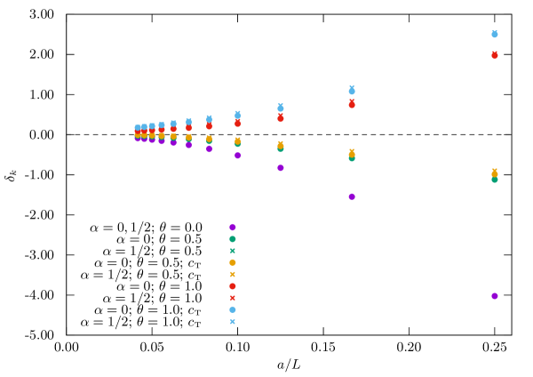
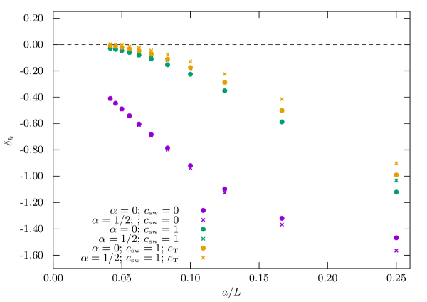
Figure 3: Upper panel: cutoff effects as a function of $a/L$ for the various schemes considered and the $\mbox{O}(a)$ improved fermion action. Results with and without operator improvement are provided. Lower panel: zoom-in displaying only results for the schemes with $\theta=0.5$ (which will be the one employed in the non-perturbative computation), also including those with an unimproved fermion action.

5 Non-perturbative computations

We will now present non-perturbative results for both $N_{\mathrm{\scriptstyle f}}=0$ and $N_{\mathrm{\scriptstyle f}}=2$ QCD. The simulations underlying each of the two cases are those in [25] (which in turn reproduced and extended the simulations in [7]) and [8], respectively. For $N_{\mathrm{\scriptstyle f}}=2$ simulations are performed with non-perturbatively $\mbox{O}(a)$ improved Wilson fermions, whereas in the quenched case the computation was performed both with and without $\mbox{O}(a)$ improvement, which, along with the finer lattices used, allows for a better control of the continuum limit (cf. below). A gauge plaquette action is always used. In both cases, we rely on the computation of the SF coupling and its non-perturbative running, given in [62, 7] for $N_{\mathrm{\scriptstyle f}}=0$ and [66] for $N_{\mathrm{\scriptstyle f}}=2$.

5.1 $N_{\mathrm{\scriptstyle f}}=0$

Simulation details for the quenched computation are given in [25]. Simulation parameters have been determined by tuning $\beta$ such that the value of the renormalized SF coupling is kept constant with changing $L/a$, and fixing the bare quark mass to the corresponding non-perturbatively tuned value of $\kappa_{\rm c}$. A total of fourteen values of the renormalized coupling have been considered, namely, $u=\{0.8873,$ $0.9944,$ $1.0989,$ $1.2430,$ $1.3293,$ $1.4300,$ $1.5553,$ $1.6950,$ $1.8811,$ $2.1000,$ $2.4484,$ $2.7700,$ $3.1110,$ $3.4800\}$, corresponding to fourteen different physical lattice lengths $L$. In all cases the renormalization constants $Z_{\rm\scriptscriptstyle T}$ are determined, in the two schemes given by $\alpha=0,1/2$, on lattices of sizes $L/a=\{6,8,12,16\}$ and $2L/a=\{12,16,24,32\}$, which allows for the determination of $\Sigma_{\rm\scriptscriptstyle T}(u,a/L)$ at four values of the lattice spacing.

As mentioned above, two separate computations have been performed, with and without an $\mbox{O}(a)$ improved fermion action with a non-perturbatively determined $c_{\rm sw}$ coefficient. This allows to improve our control over the continuum limit extrapolation for $\sigma_{\rm\scriptscriptstyle T}$, by imposing a common result for both computations based on universality. It is important to note that the gauge ensembles for the improved and unimproved computations are different, and therefore the corresponding results are fully uncorrelated. Another important observation is that the $c_{\rm\scriptscriptstyle T}$ coefficient for the $\mbox{O}(a)$ improvement counterterm of the tensor current is not known non-perturbatively, but only to leading order in perturbation theory. In our computation of $Z_{\rm\scriptscriptstyle T}$ for $N_{\mathrm{\scriptstyle f}}=0$ we have thus never included the improvement counterterm in the renormalization condition, even when the action is improved, and profit only from the above universality constraint to control the continuum limit, as we will discuss in detail below. The resulting numerical values of the renormalization constants and SSFs are reported in Tables 4 and 5.

5.1.1 Continuum extrapolation of SSFs

As discussed above, the continuum limit for $\Sigma_{\rm\scriptscriptstyle T}$ is controlled by studying the scaling of the results obtained with and without an $\mbox{O}(a)$ improved actions. To that respect, we first check that universality holds within our precision, by performing independent continuum extrapolations of both datasets. Given the absence of the $c_{\rm\scriptscriptstyle T}$ counterterm, we always assume that the continuum limit is approached linearly in $a/L$, and parametrize

$$\Sigma_{\rm\scriptscriptstyle T}^{c_{\rm sw}=0}(u,a/L)=\sigma_{\rm\scriptscriptstyle T}^{c_{\rm sw}=0}(u)+\rho_{\rm\scriptscriptstyle T}^{c_{\rm sw}=0}(u)\frac{a}{L}\,,$$ (5.51)

$$\Sigma_{\rm\scriptscriptstyle T}^{c_{\rm sw}={\rm NP}}(u,a/L)=\sigma_{\rm\scriptscriptstyle T}^{c_{\rm sw}={\rm NP}}(u)+\rho_{\rm\scriptscriptstyle T}^{c_{\rm sw}={\rm NP}}(u)\frac{a}{L}\,.$$ (5.52)

We observe that, in general, fits that drop the coarsest lattice, corresponding to the step $L/a=6\rightarrow 12$, are of better quality; when the $\Sigma_{\rm\scriptscriptstyle T}(L/a=6)$ datum is dropped, $\sigma_{\rm\scriptscriptstyle T}^{c_{\rm sw}=0}(u)$ and $\sigma_{\rm\scriptscriptstyle T}^{c_{\rm sw}={\rm NP}}(u)$ always agree within $\sim 1\sigma$. The slopes $\rho_{\rm\scriptscriptstyle T}^{c_{\rm sw}={\rm NP}}(u)$ are systematically smaller than $\rho_{\rm\scriptscriptstyle T}^{c_{\rm sw}=0}(u)$, showing that the bulk of the leading cutoff effects in the tensor current is subtracted by including the Sheikholeslami-Wohlert (SW) term in the action.

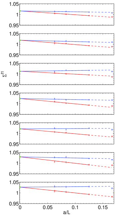
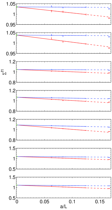
Figure 9: Continuum limit extrapolations of the $N_{\mathrm{\scriptstyle f}}=0$ SSF for the renormalization scheme $\alpha=0$. Blue (red) points correspond to results with the $\mbox{O}(a)$ improved (unimproved) action, respectively.

We thus proceed to obtain our best estimate for $\sigma_{\rm\scriptscriptstyle T}(u)$ from a constrained extrapolation, where we set $\sigma_{\rm\scriptscriptstyle T}^{c_{\rm sw}=0}(u)=\sigma_{\rm\scriptscriptstyle T}^{c_{\rm sw}={\rm NP}}(u)=\sigma_{\rm\scriptscriptstyle T}(u)$ in Eq. (5.51), and drop the $L/a=6\rightarrow 12$ step from the fit. The results for both schemes are provided in Table 6, and illustrated in Figs. 9, 10.

5.1.2 Fits to continuum step-scaling functions

In order to compute the RG running of the operator in the continuum limit, we fit the continuum-extrapolated SSFs to a functional form in $u$. The simplest choice, motivated by the perturbative expression for $\gamma_{\rm\scriptscriptstyle T}$ and $\beta$, and assuming that $\sigma_{\rm\scriptscriptstyle T}$ is a smooth function of the renormalized coupling within the covered range of values of the latter, is a polynomial of the form

$$\sigma_{\rm\scriptscriptstyle T}(u)=1+p_{1}u+p_{2}u^{2}+p_{3}u^{3}+p_{4}u^{4}+\dots\,.$$ (5.53)

The perturbative prediction for the first two coefficients of Eq. (5.53) reads

$$p_{1}^{\rm\scriptscriptstyle pert}= \gamma_{\rm\scriptscriptstyle T}^{(0)}\log(2)\,,$$ (5.54)

$$p_{2}^{\rm\scriptscriptstyle pert}= \gamma_{\rm\scriptscriptstyle T}^{(1)}\log(2)+\left[\frac{(\gamma_{\rm\scriptscriptstyle T}^{(0)})^{2}}{2}+b_{0}\gamma_{\rm\scriptscriptstyle T}^{(0)}\right](\log(2))^{2}\,.$$ (5.55)

Note, in particular, that perturbation theory predicts a dependence on $N_{\mathrm{\scriptstyle f}}$ only at ${\cal O}(u^{2})$.

We have considered various fit ansätze, exploring combinations of the order of the polynomial and possible perturbative constraints, imposed by fixing either $p_{1}$ or both $p_{1}$ and $p_{2}$ to the values in Eqs. (5.54,5.55). We always take as input the results from the joint $c_{\rm sw}=0$ and $c_{\rm sw}={\rm NP}$ extrapolation, discussed above. The results for the various fits are shown in Table 7. All the fits result in a good description of the non-perturbative data, with values of $\chi^{2}/{\rm d.o.f.}$ close to unity and little dependence on the ansatz. The coefficients of powers larger than $u^{3}$ are consistently compatible with zero within one standard deviation. We quote as our preferred fit the one that fixes $p_{1}$ to its perturbative value, and reaches ${\cal O}(u^{3})$ (fit B in Table 7). This provides an adequate description of the non-perturbative data, without artificially decreasing the goodness-of-fit by including several coefficients with large relative errors (cf., e.g., fit E). The result for $\sigma_{\rm\scriptscriptstyle T}$ from fit B in our two schemes is illustrated in Fig. 4. It is also worth pointing out that the value for $p_{2}$ obtained from fits A and B is compatible with the perturbative prediction within $1$ and $1.5$ standard deviations, respectively, for the two schemes; this reflects the small observed departure of $\sigma_{\rm\scriptscriptstyle T}$ from its two-loop value until the region $u\gtrsim 2$ is reached, cf. Fig. 4.

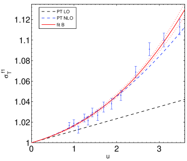
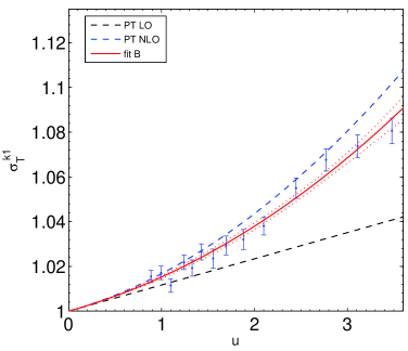
Figure 4: $N_{\mathrm{\scriptstyle f}}=0$ continuum-extrapolated SSFs in the schemes $\alpha=0$ (left) and $\alpha=1/2$ (right), and their fitted functional forms following fit B in Table 7. The one- and two-loop perturbative predictions are also shown for comparison.

5.1.3 Determination of the non-perturbative running factor

Once a given fit for $\sigma_{\rm\scriptscriptstyle T}$ is chosen, it is possible to compute the running between two well-separated scales through a finite-size recursion. The latter is started from the smallest value of the energy scale $\mu_{\rm\scriptscriptstyle had}=L_{\rm\scriptscriptstyle had}^{-1}$, given by the largest value of the coupling for which $\sigma_{\rm\scriptscriptstyle T}$ has been computed, viz.

$$\kern 1.0pt\overline{\kern-1.0ptg\kern 0.0pt}\kern 1.0pt^{2}(2\mu_{\rm\scriptscriptstyle had})=3.48\,.$$ (5.56)

Using as input the coupling SSF $\sigma(u)$ determined in [7], we construct recursively the series of coupling values

$$u_{k+1}=\kern 1.0pt\overline{\kern-1.0ptg\kern 0.0pt}\kern 1.0pt^{2}(2^{k+2}\mu_{\rm had})=\sigma^{-1}(u_{k})\,,\quad u_{0}=3.48\,.$$ (5.57)

This in turn allows to compute the product

$$U(\mu_{\rm\scriptscriptstyle had},\mu_{\rm\scriptscriptstyle pt})=\prod_{k=0}^{n}\sigma_{\rm\scriptscriptstyle T}(u_{k})\,,\quad\mu_{\rm\scriptscriptstyle pt}=2^{n+1}\mu_{\rm\scriptscriptstyle had}\,,$$ (5.58)

where $U$ is the RG evolution operator in Eq. (2.18), here connecting the renormalised operators at scales $\mu_{\rm\scriptscriptstyle had}$ and $2^{n+1}\mu_{\rm\scriptscriptstyle had}$. The number of iterations $n$ is dictated by the smallest value of $u$ at which $\sigma_{\rm\scriptscriptstyle T}$ is computed non-perturbatively, i.e. $u=0.8873$. We find $u_{7}=0.950(11)$ and $u_{8}=0.865(10)$, corresponding respectively to $8$ and $9$ steps of recursion. The latter involves a short extrapolation from the interval in $u$ covered by data, in a region where the SSF is strongly constrained by its perturbative asymptotics. This point is used only to test the robustness of the recursion, but is not considered in the final analysis. The values of $u_{k}$ and the corresponding running factors are given in Tables 8 and 9.

Once $\mu_{\rm\scriptscriptstyle pt}=2^{8}\mu_{\rm\scriptscriptstyle had}$ has been reached, perturbation theory can be used to make contact with the RGI operator. We thus compute the total running factor $\hat{c}(\mu)$ in Eq. (2.13) at $\mu=\mu_{\rm\scriptscriptstyle had}$ as

$$\hat{c}(\mu_{\rm\scriptscriptstyle had})=\frac{\hat{c}(\mu_{\rm\scriptscriptstyle pt})}{U(\mu_{\rm\scriptscriptstyle had},\mu_{\rm\scriptscriptstyle pt})}\,,$$ (5.59)

where $\hat{c}(\mu_{\rm\scriptscriptstyle pt})$ is computed using the highest available orders for $\gamma$ and $\beta$ in our schemes (NLO and NNLO, respectively). In order to assess the systematic uncertainty arising from the use of perturbation theory, we have performed two crosschecks:

1. Perform the matching to perturbation theory at all the points in the recursion, and check that the result changes within a small fraction of the error.

2. Match to perturbation theory using different combinations of perturbative orders in $\gamma$ and $\beta$: other than our NLO/NNLO preferred choice, labeled “$2/3$” — after the numbers of loops — in Tables 8 and 9, we have used matchings at $1/2$-, $2/2$-, and $3/3$-loop order, where in the latter case we have employed a mock value of the NNLO anomalous dimension given by $\gamma^{(2)}\equiv(\gamma^{(1)})^{2}/\gamma^{(0)}$ as a means to have a guesstimate of higher-order truncation uncertainties.

We thus quote as our final numbers

$$\begin{split}\left.\hat{c}(\mu_{\rm\scriptscriptstyle had})\right|_{N_{\mathrm{\scriptstyle f}}=0}&=0.9461(95)\,,\quad\mbox{scheme~{}}\alpha=0\,;\\ \left.\hat{c}(\mu_{\rm\scriptscriptstyle had})\right|_{N_{\mathrm{\scriptstyle f}}=0}&=1.0119(83)\,,\quad\mbox{scheme~{}}\alpha=1/2\,.\end{split}$$ (5.60)

In Fig. 5 we plot the non-perturbative running of the operator in our two schemes, obtained by running backwards from the perturbative matching point corresponding to the renormalized coupling $u_{7}=0.950(11)$. with our non-perturbative $\sigma_{\rm\scriptscriptstyle T}$, and compare it with perturbation theory. In order to set the physical scale corresponding to each value of the coupling, we have used $\Lambda_{\rm\scriptscriptstyle SF}/\mu_{\rm\scriptscriptstyle had}=0.422(32)$, from [7]. The latter work also provides the value of $\mu_{\rm\scriptscriptstyle had}$ in units of the Sommer scale $r_{0}$ [67], viz. $(2r_{0}\mu_{\rm\scriptscriptstyle had})^{-1}=0.718(16)$ — which, using $r_{0}=0.5~{}{\rm fm}$, translates into $\mu_{\rm\scriptscriptstyle had}=274(6)~{}{\rm MeV}$. It is important to stress that the results in Eq. (5.60) are given in the continuum, and therefore do not contain any dependence on the regularization procedures employed to obtain them.

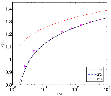
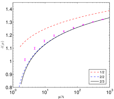
Figure 5: Running of the tensor current for $N_{\mathrm{\scriptstyle f}}=0$ in the schemes $\alpha=0$ (left) and $\alpha=1/2$ (right), compared to perturbative predictions using the $1/2$-, $2/2$-, and $2/3$-loop values for $\gamma_{\rm\scriptscriptstyle T}/\beta$.

5.1.4 Hadronic matching

The final piece required for a full non-perturbative renormalization is to compute renormalization constants at the hadronic scale $\mu_{\rm\scriptscriptstyle had}$ within the interval of values of the bare gauge coupling covered by non-perturbative simulations in large, hadronic volumes. We have thus proceeded to obtain $Z_{\rm\scriptscriptstyle T}$ at four values of the bare coupling, $\beta=\{6.0129$,$6.1628$,$6.2885$,$6.4956\}$, tuned to ensure that $L$ — and hence the renormalized SF coupling — stays constant when $L/a=\{8,10,12,16\}$, respectively. The results, both with and without $\mbox{O}(a)$ improvement, are provided in Tables 10 and 11. These numbers can be multiplied by the corresponding value of the running factor in Eq. (5.60) to obtain the quantity

$$\hat{Z}_{\rm\scriptscriptstyle T}(g_{0}^{2})=\hat{c}(\mu_{\rm\scriptscriptstyle had})Z_{\rm\scriptscriptstyle T}(g_{0}^{2},a\mu_{\rm\scriptscriptstyle had})\,,$$ (5.61)

which relates bare and RGI operators for a given value of $g_{0}^{2}$. They are quoted in Table 12; it is important to stress that the results are independent of the scheme within the $\sim 1\%$ precision of our computation — as they should, since the scheme dependence is lost at the level of RGI operators, save for the residual cutoff effects which in this case are not visible within errors. A second-order polynomial fit to the dependence of the results in $\beta$

$$\hat{Z}_{\rm\scriptscriptstyle T}(g_{0}^{2})=z_{0}+z_{1}(\beta-6)+z_{2}(\beta-6)^{2}$$ (5.62)

for the numbers obtained from the scheme $\alpha=1/2$, which turns out to be slightly more precise, yields

$$\begin{split}c_{\rm sw}={\rm NP}:&\quad z_{0}=0.9814(9)\,,\quad z_{1}=0.138(8)\,,\quad z_{2}=-0.06(2)\,;\\ c_{\rm sw}=0:&\quad z_{0}=0.8943(4)\,,\quad z_{1}=0.127(3)\,,\quad z_{2}=-0.024(6)\,,\end{split}$$ (5.63)

with correlation matrices among the fit coefficients

$$\begin{split}C[c_{\rm sw}={\rm NP}]&=\left(\begin{array}[]{rrr}1.000&-0.766&0.605\\ -0.766&1.000&-0.955\\ 0.605&-0.955&1.000\\ \end{array}\right)\,,\\[8.61108pt] C[c_{\rm sw}=0]&=\left(\begin{array}[]{rrr}1.000&-0.768&0.615\\ -0.768&1.000&-0.960\\ 0.615&-0.960&1.000\\ \end{array}\right)\,.\end{split}$$ (5.64)

These continuous form can be obtained to renormalize bare matrix elements, computed with the appropriate action, at any convenient value of $\beta$.

5.2 $N_{\mathrm{\scriptstyle f}}=2$

In this case all our simulations were performed using an $\mbox{O}(a)$ improved Wilson action, with the SW coefficient $c_{\rm sw}$ determined in[68]. Renormalization constants have been computed at six different values of the SF renormalized coupling $u=\{0.9703$,$1.1814$,$1.5078$,$2.0142$,$2.4792$,$3.3340\}$, corresponding to six different physical lattice lengths $L$. For each physical volume, three different values of the lattice spacing have been simulated, corresponding to lattices with $L/a=6,8,12$ and the double steps $2L/a=12,16,24$, for the computation of the renormalization constant $Z_{\rm\scriptscriptstyle T}(g_{0},a/L)$. All simulational details, including those referring to the tuning of $\beta$ and $\kappa$, are provided in [8].

Concerning $\mbox{O}(a)$ improvement, the configurations at the three weaker values of the coupling were produced using the one-loop perturbative estimate of $c_{\rm t}$ [21], while for the three stronger couplings the two-loop value [69] was used. In addition, for $L/a=6$, $\beta=7.5420$ and $L/a=8$, $\beta=7.7206$ separate simulations were performed with the one- and two-loop value of $c_{\rm t}$, which results in two different, uncorrelated ensembles, with either value of $c_{\rm t}$, being available for $u=1.5078$. For $\tilde{c}_{\rm t}$ the one-loop value is used throughout. Finally, since, contrary to the quenched case, we do not have two separate (improved and unimproved) sets of simulations to control the continuum limit, we have included in our analysis the improvement counterterm to the tensor current, with the one-loop value of $c_{\rm\scriptscriptstyle T}$ [61].

The resulting values for the renormalization constants $Z_{\rm\scriptscriptstyle T}$ and the SSF $\Sigma_{\rm\scriptscriptstyle T}$ are listed in Table 13. The estimate of autocorrelation times has been computed using the “Gamma Method” of [70].

5.2.1 Continuum extrapolation of SSFs

In this case, our continuum limit extrapolations will assume an $\mbox{O}(a^{2})$ scaling of $\Sigma_{\rm\scriptscriptstyle T}$. This is based on the fact that we implement $\mbox{O}(a)$ improvement of the action (up to small ${\cal O}(ag_{0}^{4})$ effects in $\tilde{c}_{\rm t}$ and ${\cal O}(ag_{0}^{4})$ or ${\cal O}(ag_{0}^{6})$ in $c_{\rm t}$, cf. above); and that the residual ${\cal O}(ag_{0}^{4})$ effects associated to the use of the one-loop perturbative value for $c_{\rm\scriptscriptstyle T}$ can be expected to be small, based on the findings discussed above for $N_{\mathrm{\scriptstyle f}}=0$. Our ansatz for a linear extrapolation in $a^{2}$ is thus of the form

$$\Sigma_{\rm\scriptscriptstyle T}(u,a/L)=\sigma_{\rm\scriptscriptstyle T}(u)+\rho_{\rm\scriptscriptstyle T}(u)\left(\frac{a}{L}\right)^{2}\,.$$ (5.65)

Furthermore, in order to ameliorate the scaling we subtract the leading perturbative cutoff effects that have been obtained in Sec. 4, by rescaling our data for $\Sigma_{\rm\scriptscriptstyle T}$ as

$$\Sigma_{\rm\scriptscriptstyle T}^{\prime}(u,a/L)=\frac{\Sigma_{\rm\scriptscriptstyle T}(u,a/L)}{1+u\delta_{k}(a/L)\gamma_{\rm\scriptscriptstyle T}^{(0)}\log(2)}\,,$$ (5.66)

where the values of the relative cutoff effects $\delta_{k}(a/L)$ are taken from Table 3. Continuum extrapolations are performed both taking $\Sigma_{\rm\scriptscriptstyle T}$ and the one-loop improved $\Sigma_{\rm\scriptscriptstyle T}^{\prime}$ as input; the two resulting continuum limits are provided in Tables 14 and 15, respectively. As showed in Fig. B, the effect of including the perturbative improvement is in general non-negligible only for our coarsest $L/a=6$ lattices. The slope of the continuum extrapolation is decreased by subtracting the perturbative cutoff effects at weak coupling, but for $u\gtrsim 2$ the quality of the extrapolation does not change significantly, and the slope actually flips sign. The $u=1.5078$ case is treated separately, and a combined extrapolation to the continuum value is performed using the independent simulations carried out with the two different values of $c_{\rm t}$. We quote as our best results the extrapolations obtained from $\Sigma_{\rm\scriptscriptstyle T}^{\prime}$.

5.2.2 Fits to continuum step-scaling functions

Here we follow exactly the same strategy described above for $N_{\mathrm{\scriptstyle f}}=0$, again considering several fit ansätze by varying the combination of the order of the polynomial and the number of coefficients fixed to their perturbative values. The results are listed in Table 16. As in the quenched case, we quote as our preferred result the fit obtained by fixing the first coefficient to its perturbative value and fitting through $\mathcal{O}(u^{3})$ (fit B). The resulting fit, as well as its comparison to perturbative predictions, is illustrated in Fig. 6.

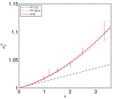
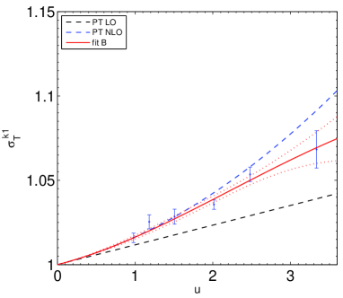
Figure 6: SSF for $N_{\mathrm{\scriptstyle f}}=2$ in the scheme $\alpha=0$ (left) and $\alpha=1/2$ (right), compared with the LO and NLO perturbative predictions.

5.2.3 Non-perturbative running

Using as input the continuum SSFs, we follow the same strategy as in the quenched case to recursively compute the running between low and high energy scales. In this case the lowest scale reached in the recursion, following [8], is given by $\kern 1.0pt\overline{\kern-1.0ptg\kern 0.0pt}\kern 1.0pt^{2}_{\rm SF}(\mu_{\rm\scriptscriptstyle had})=4.61$. Using the coupling SSF from [66], the smallest value of the coupling that can be reached via the recursion without leaving the interval covered by data is $\kern 1.0pt\overline{\kern-1.0ptg\kern 0.0pt}\kern 1.0pt^{2}_{\rm SF}(\mu_{\rm\scriptscriptstyle pt})=1.017(10)$, corresponding to $n=7$ (i.e. a total factor scale of $2^{8}$ in energy, like in the $N_{\mathrm{\scriptstyle f}}=0$ case). The matching to the RGI at $\mu_{\rm\scriptscriptstyle pt}$ is again performed using the 2/3-loop values of the $\gamma$/$\beta$ functions, and the same checks to assess the systematics are carried out as in the quenched case. Now the value obtained for $\hat{c}(\mu_{\rm\scriptscriptstyle had})$ remains within the quoted error for all $n\geq 3$. Detailed results for the recursion in either scheme are provided in Tables 17 and 18. We quote as our final results for the running factor

$$\begin{split}\left.\hat{c}(\mu_{\rm\scriptscriptstyle had})\right|_{N_{\mathrm{\scriptstyle f}}=2}&=1.001(14)\,,\quad\mbox{scheme~{}}\alpha=0\,;\\ \left.\hat{c}(\mu_{\rm\scriptscriptstyle had})\right|_{N_{\mathrm{\scriptstyle f}}=2}&=1.053(12)\,,\quad\mbox{scheme~{}}\alpha=1/2\,.\end{split}$$ (5.67)

The running is illustrated, and compared with the perturbative prediction, in Fig. 7, where the value of $\log(\Lambda_{\rm\scriptscriptstyle SF}/\mu_{\rm\scriptscriptstyle had})=-1.298(58)$ from [8] has been used. Using $r_{0}\Lambda_{\rm\scriptscriptstyle SF}=0.30(3)$ from [66] and $r_{0}=0.50~{}{\rm fm}$, this would correspond to a value of the hadronic matching energy scale $\mu_{\rm\scriptscriptstyle had}\approx 432(50)~{}{\rm MeV}$.

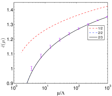
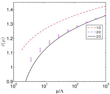
Figure 7: Running of the tensor current for $N_{\mathrm{\scriptstyle f}}=2$ in the schemes $\alpha=0$ (left) and $\alpha=1/2$ (right), compared to perturbative predictions using the $1/2$-, $2/2$-, and $2/3$-loop values for $\gamma_{\rm\scriptscriptstyle T}/\beta$.

5.2.4 Hadronic Matching

The computation of the renormalization constants at $\mu_{\rm\scriptscriptstyle had}$ needed to match bare hadronic quantities proceeds in a somewhat different way to the quenched case. The value of $Z_{\rm\scriptscriptstyle T}$ in either scheme has been computed at three values of $\beta$, namely $\beta=\{5.20,5.29,5.40\}$, again within the typical interval covered by large-volume simulations with non-perturbatively $\mbox{O}(a)$ improved fermions and a plaquette gauge action. For each of the values of $\beta$ two or three values of the lattice size $L/a$ have been simulated, corresponding to different values of $L$ and therefore to different values of the renormalized coupling. The resulting values of $Z_{\rm\scriptscriptstyle T}$ are given in Table 19.

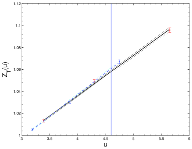
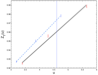
Figure 11: $N_{\mathrm{\scriptstyle f}}=2$, interpolation to $u_{\rm had}$.

The lattice size $L/a=6$ used at $\beta=5.20$ corresponds within errors to $L=1/\mu_{\rm\scriptscriptstyle had}$; for the other two values of $\beta$ linear interpolations can be performed to obtain $Z_{\rm\scriptscriptstyle T}$ at the correct value $u=4.610$; examples of such interpolations are illustrated in Fig. 11. The resulting values of $Z_{\rm\scriptscriptstyle T}$ can then be multiplied times the running factors in Eq. (5.67) to obtain the RGI renormalization factors for each $\beta$. The result is provided in Table 20. In this case the $g_{0}^{2}$ dependence is barely visible within the quoted errors, and the expected scheme independence holds only up to $\sim 3\sigma$.

6 Conclusions

In this work we have set up the strategy for a non-perturbative determination of the renormalization constants and anomalous dimension of tensor currents in QCD using SF techniques, and obtained results for $N_{\mathrm{\scriptstyle f}}=0$ and $N_{\mathrm{\scriptstyle f}}=2$. In the former case we employed both $\mbox{O}(a)$ improved and unimproved Wilson fermions, and simulations were performed at four values of the lattice spacing for each of the fourteen different values of the renormalization scale, resulting in an excellent control of the continuum limit. For $N_{\mathrm{\scriptstyle f}}=2$ our simulations were carried out with $\mbox{O}(a)$ improved fermions, at only three values of the lattice for each of the six renormalization scales. The precision of the running factors up to the electroweak scale in the schemes that allow for higher precision is $0.9\%$ and $1.1\%$, respectively. The somewhat limited quality of our $N_{\mathrm{\scriptstyle f}}=2$ dataset, however, could result in the quoted uncertainty for that case not being fully free of unquantified systematics. We have also provided values of renormalization constants at the lowest energy scales reached by the non-perturbative running, which allows to match bare matrix elements computed with non-perturbatively $\mbox{O}(a)$ improved Wilson fermions and the Wilson plaquette gauge action.

As part of the ALPHA programme, we are currently completing a similar study in $N_{\mathrm{\scriptstyle f}}=3$ QCD [37], that builds upon a high-precision determination of the strong coupling [34, 35, 36] and mass anomalous dimension [9, 10, 22]. Preliminary results indicate that a precision $\sim 1\%$ for the running to low-energy scales is possible even for values of the hadronic matching scale well below the one reached for $N_{\mathrm{\scriptstyle f}}=2$. This is an essential ingredient in order to obtain matrix elements of phenomenological interest with fully controlled uncertainties and target precisions in the few percent ballpark.

A Perturbative improvement

The improvement coefficient $c_{\rm\scriptscriptstyle T}$ for the tensor current can, by definition, be determined by requiring an $\mbox{O}(a)$ improved approach to the continuum of the renormalized correlation function at any given order in perturbation theory. As discussed in the main text, the computation of $c_{\rm\scriptscriptstyle T}$ to one loop has been carried out in [61]; here we reproduce it, mainly as a crosscheck of our perturbative setup.

We introduce the following notation for the renormalized tensor correlator ${k_{\rm\scriptscriptstyle T}}_{\rm\scriptscriptstyle;R}$ in the chiral limit evaluated with SF boundary conditions at $x_{0}=T/2$,

$$h_{\rm\scriptscriptstyle T}(\theta,a/L)\equiv{k_{\rm\scriptscriptstyle T}}_{\rm\scriptscriptstyle;R}(T/2)\,.$$ (A.68)

where the $\theta$ as well as the $a/L$ dependence have been made explicit. The one-loop expansion reads

$$h_{\rm\scriptscriptstyle T}=k_{\rm\scriptscriptstyle T}^{(0)}(T/2)+\kern 1.0pt\overline{\kern-1.0ptg\kern 0.0pt}\kern 1.0pt^{2}\{k_{\rm\scriptscriptstyle T}^{(1)}(T/2)+\tilde{c}_{\rm t}^{(1)}{k_{\rm\scriptscriptstyle T}}_{\rm;bi}^{(0)}(T/2)+am_{0}^{(1)}\frac{\partial k_{\rm\scriptscriptstyle T}^{(0)}(T/2)}{\partial m_{0}}+\\ \left(Z_{\rm\scriptscriptstyle T}^{(1)}+2Z_{\xi}^{(1)}\right)k_{\rm\scriptscriptstyle T}^{(0)}(T/2)+c_{\rm\scriptscriptstyle T}^{(1)}\tilde{\partial}_{0}k_{\rm\scriptscriptstyle V}^{(0)}(T/2)\}+\mathcal{O}(\kern 1.0pt\overline{\kern-1.0ptg\kern 0.0pt}\kern 1.0pt^{4})\,,$$ (A.69)

where $Z_{\xi}$ is the renormalization constant of the boundary fermionic fields, and $c_{\rm\scriptscriptstyle T}$ is the coefficient we are interested in, providing the $\mbox{O}(a)$ improvement of the operator. In order to determine $c_{\rm\scriptscriptstyle T}^{(1)}$ we have adopted two different strategies.

The first one proceeds by imposing the condition

$$\frac{h_{\rm\scriptscriptstyle T}(\theta,a/L)}{h_{\rm\scriptscriptstyle T}(0,a/L)}={\rm const}+\mathcal{O}(a^{2})\,.$$ (A.70)

With some trivial algebra, and observing that $\tilde{\partial}_{0}k_{\rm\scriptscriptstyle V}^{(0)}(\theta=0)=0$, we end up with the relation

$$\frac{\bar{k}_{\rm\scriptscriptstyle T}^{(1)}(\theta,a/L)}{k_{\rm\scriptscriptstyle T}^{(0)}(\theta,a/L)}-\frac{\bar{k}_{\rm\scriptscriptstyle T}^{(1)}(0,a/L)}{k_{\rm\scriptscriptstyle T}^{(0)}(0,a/L)}=-c_{\rm\scriptscriptstyle T}^{(1)}\frac{\tilde{\partial}_{0}k_{\rm\scriptscriptstyle V}^{(0)}(\theta,a/L)|_{x_{0}=T/2}}{k_{\rm\scriptscriptstyle T}^{(0)}(\theta,a/L)}\,,$$ (A.71)

where $\bar{k}_{\rm\scriptscriptstyle T}$ is a shorthand notation for the correlator including the subtraction of the boundary and mass $\mbox{O}(a)$ terms. The divergent part of $Z_{\rm\scriptscriptstyle T}^{(1)}$, as well as of $Z_{\xi}$, cancel out in the ratio, since they are independent of $\theta$ at one loop. Following [71], in order to remove the constant term on the r.h.s. of Eq. (A.70) — which is indeed proportional to the difference of the finite parts at two different values of $\theta$ — we take a symmetric derivative in $L$, defined as

$$\tilde{\partial}_{L}f(L)=\frac{1}{2a}\left[f(L+a)-f(L-a)\right]\,,$$ (A.72)

and apply it to both sides of Eq. (A.71), obtaining

$$R(\theta,a/L)=-\frac{\tilde{\partial}_{L}C(L)}{\tilde{\partial}_{L}A(L)}=c_{\rm\scriptscriptstyle T}^{(1)}+\mbox{O}(a)\,,$$ (A.73)

with $C(L)$ as the l.h.s of Eq. (A.71), and $A(L)$ the r.h.s. without the term with $c_{\rm\scriptscriptstyle T}^{(1)}$.

As a second strategy to determine $c_{\rm\scriptscriptstyle T}$ to one loop, one can exploit the tree-level identities obtained in [71], which relate $k_{\rm\scriptscriptstyle V}^{(0)},k_{\rm\scriptscriptstyle T}^{(0)},f_{\rm\scriptscriptstyle A}^{(0)}$ and $f_{\rm\scriptscriptstyle P}^{(0)}$, and impose

$$\bar{k}_{\rm\scriptscriptstyle T}^{(1)}+\frac{1}{3}\bar{f}_{\rm\scriptscriptstyle P}^{(1)}-\frac{2}{3}\bar{f}_{\rm\scriptscriptstyle A}^{(1)}+Z_{\rm\scriptscriptstyle T}^{(1)}k_{\rm\scriptscriptstyle T}^{(0)}+\frac{1}{3}Z_{\rm\scriptscriptstyle P}^{(1)}f_{\rm\scriptscriptstyle P}^{(0)}+\\ c_{\rm\scriptscriptstyle T}^{(1)}\tilde{\partial}_{0}k_{\rm\scriptscriptstyle V}^{(0)}|_{x_{0}=T/2}-\frac{2}{3}c_{A}^{(1)}\tilde{\partial}_{0}f_{\rm\scriptscriptstyle P}^{(0)}|_{x_{0}=T/2})={\rm const}+\mathcal{O}(a^{2}).$$ (A.74)

After some simple algebra we find

$$F(\theta,a/L)\equiv-\frac{\tilde{\partial}_{L}C(L)}{\tilde{\partial}_{L}A(L)}+c_{A}^{(1)}=c_{\rm\scriptscriptstyle T}^{(1)}+\mbox{O}(a)\,,$$ (A.75)

where now

$$C(L)=\bar{k}_{\rm\scriptscriptstyle T}^{(1)}(L/a)+\frac{1}{3}\bar{f}_{\rm\scriptscriptstyle P}^{(1)}(L/a)-\frac{2}{3}\bar{f}_{\rm\scriptscriptstyle A}^{(1)}(L/a)+\\ \frac{8}{3(4\pi^{2})}\log(L/a)[k_{\rm\scriptscriptstyle T}^{(0)}(L/a)-f_{\rm\scriptscriptstyle P}^{(0)}(L/a)]\,,$$ (A.76)

$$A(L)=\tilde{\partial}_{0}f_{\rm\scriptscriptstyle P}^{(0)}(T/2)\,.$$ (A.77)

Using the results for $c_{\rm\scriptscriptstyle A}^{(1)}$ quoted in [71], we reproduce within errors the value quoted in [61], which reads

$$c_{\rm\scriptscriptstyle T}^{(1)}=0.00896(1)C_{\rm F}\,.$$ (A.78)

The comparison between our determination and the one in [61] is displayed in Fig. A. In all cases, the continuum extrapolation has been performed using similar techniques to the one employed for the finite part of renormalization constants (see App. B).

figureExtraction of $c_{\rm\scriptscriptstyle T}^{(1)}$, compared with the result in [61].

B Continuum extrapolations in perturbation theory

In this appendix we summarize the techniques used to extrapolate our perturbative computations to $a/L\to 0$, a necessary step in order to obtain scheme-matching and improvement coefficients. Our approach is essentially an application to the present context of the techniques discussed in Appendix D of [69], which have been applied in a number of cases, see e.g. [26].

The typical outcome of a perturbative computation is a linear combination of one-loop Feynman diagrams, e.g. the one yielding the one-loop coefficient $Z^{(1)}$ of a renormalization constant, for $N$ values $\{l_{1},\dots,l_{N}\}$ of the variable $l=L/a$. We consider the quantity to be a function of $l$ only. It is possible to identify all divergences appearing in the quantity of interest at one-loop, which in general means linear divergences related to the additive renormalization of the quark masses proportional to the one-loop critical mass $m_{\rm cr}^{(1)}$, and the logarithmic divergences proportional to the (one-loop) anomalous dimension. The latter is particularly relevant for the present analysis, since it allows to check the consistency of the fitting procedure and provides a natural criterion for the choice of the best fitting ansatz. In the following we consider finite quantities, since the leading divergence is subtracted, and the critical mass is appropriately tuned. Considering $F(l)$ as a generic one-loop interesting quantity, following [69] we conservatively assign the error

$$\delta F(l)=\epsilon(l)|F(l)|\,,\epsilon(l)=\left(\frac{l}{2}\right)^{3}\times 10^{-14}\,,$$ (B.79)

since in this case the computation has been carried out in double precision. As expected, the asymptotic behaviour is (cf. Eq. (4.45))

$$F(l)=r_{0}+\sum_{k=1}^{n}\frac{1}{l^{n}}(r_{k}+s_{k}{\rm ln}(l))+R_{n}(l)$$ (B.80)

with a residue $R_{n}(l)$ that decreases faster than any of the terms in the sum as $l\to\infty$. In order to determine the coefficients $(r_{k},s_{k})$ we define as our likelihood function a $\chi^{2}$ given by

$$\chi^{2}=(F-f\xi)^{T}W(F-f\xi)\,,$$ (B.81)

where $F$ and $\xi$ are the $N-$column vectors $F=(F(l_{1}),\dots,F(l_{N}))^{T}$ and $(2n+1)-$column vector $\xi=(r_{0},r_{1},\dots,r_{n},s_{1},\dots,s_{0})^{T}$, $f$ is the $N\times(2n+1)$ matrix

$$f=\begin{pmatrix}1&l_{1}^{-1}&\dots&l_{1}^{-n}&l_{1}^{-1}{\rm ln}(l_{1})&\dots&l_{1}^{-n}{\rm ln}(l_{1})\\ 1&l_{2}^{-1}&\dots&l_{2}^{-n}&l_{2}^{-1}{\rm ln}(l_{2})&\dots&l_{2}^{-n}{\rm ln}(l_{2})\\ \vdots&\vdots&\vdots&\vdots&\vdots&\vdots&\vdots\\ 1&l_{N}^{-1}&\dots&l_{N}^{-n}&l_{N}^{-1}{\rm ln}(l_{N})&\dots&l_{N}^{-n}{\rm ln}(l_{N})\end{pmatrix}\,,$$ (B.82)

and $W$ is in general a matrix with weights which, as suggested in [69], is omitted from the actual $\chi^{2}$ used. The minimum condition for our likelihood function is given by

$$f\xi=PF\,,$$ (B.83)

where we are assuming that $2n+1<N$, and $P$ is the projector to the subspace spanned by the linearly independent column-vectors of $f$. A convenient and numerically stable way to solve Eq. (B.83) is the Singular Value Decomposition of $f$

$$f=USV^{T}\,,$$ (B.84)

where $U$ is an $N\times(2n+1)$ matrix such that

$$U^{T}U=\mathbf{1}\,\quad\,UU^{T}=P\,,$$ (B.85)

$S$ is a diagonal and $V$ is an orthonormal $(2n+1)\times(2n+1)$ matrix. Inserting Eq. (B.84) into Eq. (B.83) one has

$$\xi=VS^{-1}U^{T}F\,.$$ (B.86)

Finally the uncertainty of the results $\xi_{k}$ is estimated to be

$$(\delta\xi_{k})^{2}=\sum_{l=1}^{N}[(VS^{-1}U^{T})_{kl}]^{2}(\delta F_{l})^{2}\,,$$ (B.87)

with $\delta F_{k}=F(l_{k})$. In order to avoid giving excessive weight to the coarsest lattices, we considered several possible fit ranges $[l_{\rm min},l_{\rm max}]$, where $l_{\rm max}=48$ and $l_{\rm min}$ is changed from $4$ to $20$. In order to account for a better description of the dependence on $l$ we explored different values of $n$ from $1$ to $4$.

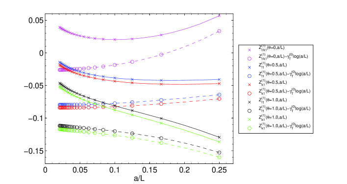
Figure 8: One-loop renormalization constants for the three values of $\theta=0,0.5,1$. The $a/L$ dependence both before and after the subtraction of the leading logarithmic divergence is shown.

In particular, concerning the fit for the extraction of the finite parts, we chose as best ansatz the one reproducing the coefficient of the LO anomalous dimension $\gamma_{T}^{(0)}$. In particular for the Wilson action we find $s_{0}/\gamma_{\rm\scriptscriptstyle T}^{(0)}=0.998(5)$ for both $f_{1}$ and $k_{1}$ schemes using $n=3$ starting with $L/a=16$ as the smallest lattice. In the case with clover improvement of the action for the three values of $\theta=0$ for $n=3$ $L/a=14$ we have $\gamma_{\rm\scriptscriptstyle T}^{(0)}/s_{0}=1.001(3)$; for $\theta=0.5$, $n=3$, and $L/a=10$, $\gamma_{\rm\scriptscriptstyle T}^{(0)}/s_{0}=1.000(6)$; and finally, for $\theta=1.0$, $n=3$, and $L/a=10$, $\gamma_{T}^{(0)}/s_{0}=1.000(3)$.

$L/a$	[0.0,0,1,1l,*]	[0.0,1/2,1,1l,*]	[1.0,0,1,1l,0]	[1.0,1/2,1,1l,0]	[1.0,0,1,1l,1l]	[1.0,1/2,1,1l,1l]
4	-4.024919	-4.024919	1.973892	2.021956	2.500183	2.548247
6	-1.548675	-1.548675	0.740155	0.831017	1.079337	1.170200
8	-0.826327	-0.826327	0.400756	0.475909	0.651713	0.726867
10	-0.516240	-0.516240	0.273405	0.331519	0.472838	0.530953
12	-0.353534	-0.353534	0.209692	0.254876	0.375268	0.420452
14	-0.257339	-0.257339	0.171319	0.207105	0.312917	0.348703
16	-0.195713	-0.195713	0.145443	0.174349	0.269155	0.298061
18	-0.153857	-0.153857	0.126680	0.150454	0.236532	0.260306
20	-0.124131	-0.124131	0.112377	0.132244	0.211170	0.231037
22	-0.102261	-0.102261	0.101072	0.117905	0.190834	0.207667
24	-0.085702	-0.085702	0.091888	0.106322	0.174135	0.188570

$L/a$	[0.5,0,0,0,0]	[0.5,1/2,0,0,0]	[0.5,0,1,1l,0]	[0.5,1/2,1,1l,0]	[0.5,0,1,1l,1l]	[0.5,1/2,1,1l,1l]
4	-1.467173	-1.564753	-1.120302	-1.031861	-0.990330	-0.901889
6	-1.318718	-1.366570	-0.587012	-0.500733	-0.501419	-0.415141
8	-1.097265	-1.125110	-0.351334	-0.288400	-0.287405	-0.224471
10	-0.919572	-0.937671	-0.225979	-0.179971	-0.174931	-0.128923
12	-0.785609	-0.798283	-0.153873	-0.119221	-0.111375	-0.076724
14	-0.683546	-0.692903	-0.109513	-0.082621	-0.073108	-0.046216
16	-0.603968	-0.611155	-0.080628	-0.059210	-0.048785	-0.027367
18	-0.540470	-0.546161	-0.060930	-0.043495	-0.032633	-0.015198
20	-0.488753	-0.493370	-0.046987	-0.032532	-0.021524	-0.007069
22	-0.445879	-0.449699	-0.036813	-0.024641	-0.013668	-0.001496
24	-0.409794	-0.413007	-0.029200	-0.018813	-0.018813	0.002400

Table 3: Cutoff effects $\delta_{k}$ in tensor SSFs (see Eq. (4.50)) for various schemes and amounts of $\mbox{O}(a)$ improvement. The headers of the columns correspond to the values of the parameters $[\theta,\alpha,c_{\rm sw},\tilde{c}_{\rm t},c_{\rm\scriptscriptstyle T}]$ (“1l” refers to the one-loop value of the coefficient). For $\theta=0.0$ results at one loop are independent of the value of $\alpha$, and the contribution from $c_{\rm\scriptscriptstyle T}$ vanishes.

			Improved action				Unimproved action
$\beta~{}~{}~{}$	$L/a$	$~{}~{}~{}\bar{g}^{2}(L)$	$~{}~{}~{}~{}~{}~{}\kappa_{\rm c}$	$Z_{\rm\scriptscriptstyle T}\left(g_{0}^{2},L/a\right)$	$Z_{\rm\scriptscriptstyle T}\left(g_{0}^{2},2L/a\right)$	$\Sigma_{\rm\scriptscriptstyle T}\left(u,L/a\right)$	$~{}~{}~{}~{}~{}~{}\kappa_{\rm c}$	$Z_{\rm\scriptscriptstyle T}\left(g_{0}^{2},L/a\right)$	$Z_{\rm\scriptscriptstyle T}\left(g_{0}^{2},2L/a\right)$	$\Sigma_{\rm\scriptscriptstyle T}\left(u,L/a\right)$
10.7503	6	0.8873(5)	0.130591(4)	0.9781(7)	0.9857(12)	1.0078(14)	0.134696(7)	0.9571(8)	0.9464(11)	0.9888(14)
11.0000	8	0.8873(10)	0.130439(3)	0.9812(7)	0.9923(12)	1.0113(14)	0.134548(6)	0.9569(7)	0.9522(12)	0.9951(15)
11.3384	12	0.8873(30)	0.130251(2)	0.9878(11)	1.0022(16)	1.0146(20)	0.134277(5)	0.9605(11)	0.9618(18)	1.0014(22)
11.5736	16	0.8873(25)	0.130125(2)	0.9918(10)	1.0061(23)	1.0144(25)	0.134068(6)	0.9637(11)	0.9686(20)	1.0051(24)
10.0500	6	0.9944(7)	0.131073(5)	0.9771(7)	0.9868(14)	1.0099(16)	0.135659(8)	0.9532(10)	0.9428(12)	0.9891(16)
10.3000	8	0.9944(13)	0.130889(3)	0.9820(11)	0.9927(12)	1.0109(17)	0.135457(5)	0.9535(8)	0.9472(13)	0.9934(16)
10.6086	12	0.9944(30)	0.130692(2)	0.9896(12)	1.0047(18)	1.0153(22)	0.135160(4)	0.9590(11)	0.9624(20)	1.0035(24)
10.8910	16	0.9944(28)	0.130515(2)	0.9936(11)	1.0073(20)	1.0138(23)	0.134849(6)	0.9641(13)	0.9686(33)	1.0047(37)
9.5030	6	1.0989(8)	0.131514(5)	0.9766(9)	0.9880(15)	1.0117(18)	0.136520(5)	0.9516(10)	0.9389(14)	0.9867(18)
9.7500	8	1.0989(13)	0.131312(3)	0.9798(9)	0.9964(16)	1.0169(19)	0.136310(3)	0.9515(9)	0.9475(13)	0.9958(17)
10.0577	12	1.0989(40)	0.131079(3)	0.9874(12)	1.0048(18)	1.0176(22)	0.135949(4)	0.9574(13)	0.9581(22)	1.0007(27)
10.3419	16	1.0989(44)	0.130876(2)	0.9963(14)	1.0090(19)	1.0127(24)	0.135572(4)	0.9619(18)	0.9676(22)	1.0059(30)
8.8997	6	1.2430(13)	0.132072(9)	0.9742(6)	0.9908(12)	1.0170(14)	0.137706(5)	0.9463(11)	0.9363(14)	0.9894(19)
9.1544	8	1.2430(14)	0.131838(4)	0.9806(8)	0.9988(17)	1.0186(19)	0.137400(4)	0.9487(10)	0.9426(17)	0.9936(21)
9.5202	12	1.2430(35)	0.131503(3)	0.9885(11)	1.0062(23)	1.0179(26)	0.136855(2)	0.9537(14)	0.9558(16)	1.0022(22)
9.7350	16	1.2430(34)	0.131335(3)	0.9971(21)	1.0201(22)	1.0231(31)	0.136523(4)	0.9564(14)	0.9661(23)	1.0101(28)
8.6129	6	1.3293(12)	0.132380(6)	0.9732(9)	0.9903(17)	1.0176(20)	0.138346(6)	0.9455(12)	0.9322(13)	0.9859(19)
8.8500	8	1.3293(21)	0.132140(5)	0.9797(10)	1.0036(18)	1.0244(21)	0.138057(4)	0.9475(10)	0.9397(18)	0.9918(22)
9.1859	12	1.3293(60)	0.131814(3)	0.9914(15)	1.0089(25)	1.0177(30)	0.137503(2)	0.9534(15)	0.9572(18)	1.0040(25)
9.4381	16	1.3293(40)	0.131589(2)	0.9962(14)	1.0207(30)	1.0246(33)	0.137061(4)	0.9578(22)	0.9645(23)	1.0070(33)
8.3124	6	1.4300(20)	0.132734(10)	0.9750(7)	0.9908(14)	1.0162(16)	0.139128(11)	0.9393(12)	0.9299(15)	0.9900(20)
8.5598	8	1.4300(21)	0.132453(5)	0.9800(9)	1.0011(16)	1.0215(19)	0.138742(7)	0.9445(11)	0.9381(20)	0.9932(24)
8.9003	12	1.4300(50)	0.132095(3)	0.9897(17)	1.0188(26)	1.0294(32)	0.138120(8)	0.9532(15)	0.9574(25)	1.0044(31)
9.1415	16	1.4300(58)	0.131855(3)	0.9976(12)	1.0248(28)	1.0273(31)	0.137655(5)	0.9592(16)	0.9655(26)	1.0066(32)
7.9993	6	1.5553(15)	0.133118(7)	0.9726(7)	0.9932(21)	1.0212(23)	0.140003(11)	0.9385(13)	0.9215(15)	0.9819(21)
8.2500	8	1.5553(24)	0.132821(5)	0.9785(11)	1.0073(22)	1.0294(25)	0.139588(8)	0.9422(11)	0.9359(20)	0.9933(24)
8.5985	12	1.5533(70)	0.132427(3)	0.9927(17)	1.0204(29)	1.0279(34)	0.138847(6)	0.9532(16)	0.9575(27)	1.0045(33)
8.8323	16	1.5533(70)	0.132169(3)	0.9999(19)	1.0305(35)	1.0306(40)	0.138339(7)	0.9594(22)	0.9671(34)	1.0080(42)

Table 4: $N_{\mathrm{\scriptstyle f}}=0$ results for the renormalization constant $Z_{\rm\scriptscriptstyle P}$ and the step scaling function $\Sigma_{\rm\scriptscriptstyle T}$ for the scheme $\alpha=0$.

			Improved action				Unimproved action
$\beta~{}~{}~{}$	$L/a$	$~{}~{}~{}\bar{g}^{2}(L)$	$~{}~{}~{}~{}~{}~{}\kappa_{\rm c}$	$Z_{\rm\scriptscriptstyle T}\left(g_{0}^{2},L/a\right)$	$Z_{\rm\scriptscriptstyle T}\left(g_{0}^{2},2L/a\right)$	$\Sigma_{\rm\scriptscriptstyle T}\left(u,L/a\right)$	$~{}~{}~{}~{}~{}~{}\kappa_{\rm c}$	$Z_{\rm\scriptscriptstyle T}\left(g_{0}^{2},L/a\right)$	$Z_{\rm\scriptscriptstyle T}\left(g_{0}^{2},2L/a\right)$	$\Sigma_{\rm\scriptscriptstyle T}\left(u,L/a\right)$
7.7170	6	1.6950(26)	0.133517(8)	0.9729(10)	0.9977(7)	1.0255(13)	0.140954(12)	0.9380(13)	0.9199(18)	0.9807(24)
7.9741	8	1.6950(28)	0.133179(5)	0.9787(9)	1.0115(22)	1.0335(24)	0.140438(8)	0.9402(12)	0.9385(29)	0.9982(33)
8.3218	12	1.6950(79)	0.132756(4)	0.9953(7)	1.0268(23)	1.0316(24)	0.139589(6)	0.9505(18)	0.9616(28)	1.0117(35)
8.5479	16	1.6950(90)	0.132485(3)	1.0014(19)	1.0389(32)	1.0374(38)	0.139058(6)	0.9579(20)	0.9719(36)	1.0146(43)
7.4082	6	1.8811(22)	0.133961(8)	0.9702(10)	0.9992(8)	1.0299(13)	0.142145(11)	0.9346(14)	0.9122(18)	0.9760(24)
7.6547	8	1.8811(28)	0.133632(6)	0.9812(10)	1.0175(22)	1.0370(25)	0.141572(9)	0.9386(13)	0.9347(19)	0.9958(24)
7.9993	12	1.8811(38)	0.133159(4)	0.9980(7)	1.0317(32)	1.0338(33)	0.140597(6)	0.9498(18)	0.9559(32)	1.0064(39)
8.2415	16	1.8811(99)	0.132847(3)	1.0059(28)	1.0445(27)	1.0384(39)	0.139900(6)	0.9565(22)	0.9776(38)	1.0221(46)
7.1214	6	2.1000(39)	0.134423(9)	0.9720(12)	1.0039(9)	1.0328(16)	0.143416(11)	0.9243(16)	0.9067(21)	0.9810(28)
7.3632	8	2.1000(45)	0.134088(6)	0.9833(12)	1.0235(26)	1.0409(29)	0.142749(9)	0.9312(14)	0.9253(27)	0.9937(33)
7.6985	12	2.1000(80)	0.133599(4)	0.9995(8)	1.0427(25)	1.0432(26)	0.141657(6)	0.9480(14)	0.9564(22)	1.0089(28)
7.9560	16	2.100(11)	0.133229(3)	1.0090(21)	1.0564(27)	1.0470(35)	0.140817(7)	0.9594(22)	0.9749(35)	1.0162(43)
6.7807	6	2.4484(37)	0.134994(11)	0.9741(13)	1.0160(10)	1.0430(17)	0.145286(11)	0.9229(15)	0.9003(21)	0.9755(28)
7.0197	8	2.4484(45)	0.134639(7)	0.9866(13)	1.0301(29)	1.0441(32)	0.144454(7)	0.9318(15)	0.9256(23)	0.9933(29)
7.3551	12	2.4484(80)	0.134141(5)	1.0061(8)	1.0618(30)	1.0554(31)	0.143113(6)	0.9522(17)	0.9572(38)	1.0053(44)
7.6101	16	2.448(17)	0.133729(4)	1.0167(22)	1.0808(32)	1.0630(39)	0.142107(6)	0.9579(22)	0.9851(39)	1.0284(47)
6.5512	6	2.770(7)	0.135327(12)	0.9798(14)	1.0279(8)	1.0491(17)	0.146825(11)	0.9208(18)	0.8887(22)	0.9651(30)
6.7860	8	2.770(7)	0.135056(8)	0.9910(13)	1.0527(31)	1.0623(34)	0.145859(7)	0.9311(16)	0.9181(33)	0.9860(39)
7.1190	12	2.770(11)	0.134513(5)	1.0097(10)	1.0823(25)	1.0719(27)	0.144299(8)	0.9489(21)	0.9688(33)	1.0210(41)
7.3686	16	2.770(14)	0.134114(3)	1.0215(27)	1.1012(37)	1.0780(46)	0.143175(7)	0.9663(31)	1.0018(47)	1.0367(59)
6.3665	6	3.111(4)	0.135488(6)	0.9809(16)	1.0384(30)	1.0586(35)	0.148317(10)	0.9207(19)	0.8802(19)	0.9560(29)
6.6100	8	3.111(6)	0.135339(3)	0.9944(16)	1.0711(37)	1.0771(41)	0.147112(7)	0.9328(18)	0.9189(27)	0.9851(35)
6.9322	12	3.111(12)	0.134855(3)	1.0160(23)	1.1093(35)	1.0918(42)	0.145371(7)	0.9526(21)	0.9740(35)	1.0225(43)
7.1911	16	3.111(16)	0.134411(3)	1.0340(21)	1.1222(42)	1.0853(46)	0.144060(8)	0.9676(28)	1.0092(45)	1.0430(55)
6.2204	6	3.480(8)	0.135470(15)	0.9869(8)	1.0678(27)	1.0820(29)	0.149685(15)	0.9178(21)	0.8709(23)	0.9489(33)
6.4527	8	3.480(14)	0.135543(9)	1.0005(10)	1.0909(46)	1.0904(47)	0.148391(9)	0.9295(19)	0.9140(44)	0.9833(51)
6.7750	12	3.480(39)	0.135121(5)	1.0292(20)	1.1281(41)	1.0961(45)	0.146408(7)	0.9570(20)	0.9793(49)	1.0233(55)
7.0203	16	3.480(21)	0.134707(4)	1.0408(22)	1.1420(45)	1.0972(49)	0.145025(8)	0.9714(24)	1.0264(51)	1.0566(59)

Table 4: (continued)

			Improved action				Unimproved action
$\beta~{}~{}~{}$	$L/a$	$~{}~{}~{}\bar{g}^{2}(L)$	$~{}~{}~{}~{}~{}~{}\kappa_{\rm c}$	$Z_{\rm\scriptscriptstyle T}\left(g_{0}^{2},L/a\right)$	$Z_{\rm\scriptscriptstyle T}\left(g_{0}^{2},2L/a\right)$	$\Sigma_{\rm\scriptscriptstyle T}\left(u,L/a\right)$	$~{}~{}~{}~{}~{}~{}\kappa_{\rm c}$	$Z_{\rm\scriptscriptstyle T}\left(g_{0}^{2},L/a\right)$	$Z_{\rm\scriptscriptstyle T}\left(g_{0}^{2},2L/a\right)$	$\Sigma_{\rm\scriptscriptstyle T}\left(u,L/a\right)$
10.7503	6	0.8873(5)	0.130591(4)	0.9687(6)	0.9769(11)	1.0085(13)	0.134696(7)	0.9497(8)	0.9388(10)	0.9885(13)
11.0000	8	0.8873(10)	0.130439(3)	0.9726(6)	0.9835(11)	1.0112(13)	0.134548(6)	0.9497(7)	0.9446(11)	0.9946(14)
11.3384	12	0.8873(30)	0.130251(2)	0.9795(10)	0.9930(14)	1.0138(18)	0.134277(5)	0.9529(10)	0.9536(16)	1.0007(20)
11.5736	16	0.8873(25)	0.130125(2)	0.9839(9)	0.9974(20)	1.0137(22)	0.134068(6)	0.9561(10)	0.9603(18)	1.0044(22)
10.0500	6	0.9944(7)	0.131073(5)	0.9661(7)	0.9761(11)	1.0104(14)	0.135659(8)	0.9448(9)	0.9339(11)	0.9885(15)
10.3000	8	0.9944(13)	0.130889(3)	0.9716(9)	0.9824(10)	1.0111(14)	0.135457(5)	0.9450(8)	0.9381(11)	0.9927(14)
10.6086	12	0.9944(30)	0.130692(2)	0.9800(11)	0.9942(16)	1.0145(20)	0.135160(4)	0.9500(10)	0.9521(18)	1.0022(22)
10.8910	16	0.9944(28)	0.130515(2)	0.9845(9)	0.9974(18)	1.0131(20)	0.134849(6)	0.9554(11)	0.9590(29)	1.0038(32)
9.5030	6	1.0989(8)	0.131514(5)	0.9642(8)	0.9761(13)	1.0123(16)	0.136520(5)	0.9419(9)	0.9290(12)	0.9863(16)
9.7500	8	1.0989(13)	0.131312(3)	0.9682(8)	0.9842(13)	1.0165(16)	0.136310(3)	0.9415(8)	0.9369(11)	0.9951(14)
10.0577	12	1.0989(40)	0.131079(3)	0.9766(10)	0.9934(15)	1.0172(19)	0.135949(4)	0.9471(12)	0.9466(18)	0.9995(23)
10.3419	16	1.0989(44)	0.130876(2)	0.9859(12)	0.9975(16)	1.0118(20)	0.135572(4)	0.9518(16)	0.9568(19)	1.0053(26)
8.8997	6	1.2430(13)	0.132072(9)	0.9598(6)	0.9759(10)	1.0168(12)	0.137706(5)	0.9351(10)	0.9243(12)	0.9885(17)
9.1544	8	1.2430(14)	0.131838(4)	0.9673(7)	0.9840(14)	1.0173(16)	0.137400(4)	0.9374(9)	0.9305(15)	0.9926(19)
9.5202	12	1.2430(35)	0.131503(3)	0.9762(9)	0.9926(19)	1.0168(22)	0.136855(2)	0.9421(12)	0.9433(13)	1.0013(19)
9.7350	16	1.2430(34)	0.131335(3)	0.9849(18)	1.0057(18)	1.0211(26)	0.136523(4)	0.9453(13)	0.9530(20)	1.0081(25)
8.6129	6	1.3293(12)	0.132380(6)	0.9577(8)	0.9742(15)	1.0172(18)	0.138346(6)	0.9332(11)	0.9191(12)	0.9849(17)
8.8500	8	1.3293(21)	0.132140(5)	0.9652(8)	0.9871(15)	1.0227(18)	0.138057(4)	0.9349(9)	0.9262(15)	0.9907(19)
9.1859	12	1.3293(60)	0.131814(3)	0.9776(13)	0.9934(20)	1.0162(25)	0.137503(2)	0.9403(13)	0.9428(15)	1.0027(21)
9.4381	16	1.3293(40)	0.131589(2)	0.9832(12)	1.0055(25)	1.0227(28)	0.137061(4)	0.9456(19)	0.9504(20)	1.0051(29)
8.3124	6	1.4300(20)	0.132734(10)	0.9579(6)	0.9731(11)	1.0159(13)	0.139128(11)	0.9263(11)	0.9153(13)	0.9881(18)
8.5598	8	1.4300(21)	0.132453(5)	0.9642(8)	0.9833(13)	1.0198(16)	0.138742(7)	0.9312(10)	0.9233(17)	0.9915(21)
8.9003	12	1.4300(50)	0.132095(3)	0.9748(14)	1.0001(21)	1.0260(26)	0.138120(8)	0.9396(13)	0.9411(20)	1.0016(25)
9.1415	16	1.4300(58)	0.131855(3)	0.9835(10)	1.0085(24)	1.0254(27)	0.137655(5)	0.9452(14)	0.9497(22)	1.0048(28)
7.9993	6	1.5553(15)	0.133118(7)	0.9537(6)	0.9725(17)	1.0197(19)	0.140003(11)	0.9239(11)	0.9066(13)	0.9813(18)
8.2500	8	1.5553(24)	0.132821(5)	0.9614(9)	0.9873(18)	1.0269(21)	0.139588(8)	0.9273(10)	0.9197(17)	0.9918(21)
8.5985	12	1.5533(70)	0.132427(3)	0.9765(14)	1.0006(24)	1.0247(29)	0.138847(6)	0.9376(14)	0.9403(24)	1.0029(30)
8.8323	16	1.5533(70)	0.132169(3)	0.9837(16)	1.0102(27)	1.0269(32)	0.138339(7)	0.9441(18)	0.9499(28)	1.0061(35)

Table 5: $N_{\mathrm{\scriptstyle f}}=0$ results for the renormalization constant $Z_{\rm\scriptscriptstyle P}$ and the step scaling function $\Sigma_{\rm\scriptscriptstyle T}$ for the scheme $\alpha=1/2$.

			Improved action				Unimproved action
$\beta~{}~{}~{}$	$L/a$	$~{}~{}~{}\bar{g}^{2}(L)$	$~{}~{}~{}~{}~{}~{}\kappa_{\rm c}$	$Z_{\rm\scriptscriptstyle T}\left(g_{0}^{2},L/a\right)$	$Z_{\rm\scriptscriptstyle T}\left(g_{0}^{2},2L/a\right)$	$\Sigma_{\rm\scriptscriptstyle T}\left(u,L/a\right)$	$~{}~{}~{}~{}~{}~{}\kappa_{\rm c}$	$Z_{\rm\scriptscriptstyle T}\left(g_{0}^{2},L/a\right)$	$Z_{\rm\scriptscriptstyle T}\left(g_{0}^{2},2L/a\right)$	$\Sigma_{\rm\scriptscriptstyle T}\left(u,L/a\right)$
7.7170	6	1.6950(26)	0.133517(8)	0.9522(9)	0.9747(6)	1.0236(12)	0.140954(12)	0.9215(12)	0.9026(15)	0.9795(21)
7.9741	8	1.6950(28)	0.133179(5)	0.9599(7)	0.9887(18)	1.0300(20)	0.140438(8)	0.9234(11)	0.9204(24)	0.9968(29)
8.3218	12	1.6950(79)	0.132756(4)	0.9769(5)	1.0042(19)	1.0279(20)	0.139589(6)	0.9333(15)	0.9408(22)	1.0080(29)
8.5479	16	1.6950(90)	0.132485(3)	0.9839(16)	1.0160(26)	1.0326(31)	0.139058(6)	0.9412(17)	0.9522(31)	1.0117(38)
7.4082	6	1.8811(22)	0.133961(8)	0.9472(9)	0.9730(6)	1.0272(12)	0.142145(11)	0.9162(12)	0.8933(15)	0.9750(21)
7.6547	8	1.8811(28)	0.133632(6)	0.9597(8)	0.9912(18)	1.0328(21)	0.141572(9)	0.9197(11)	0.9129(16)	0.9926(21)
7.9993	12	1.8811(38)	0.133159(4)	0.9771(6)	1.0066(27)	1.0302(28)	0.140597(6)	0.9306(15)	0.9337(26)	1.0033(32)
8.2415	16	1.8811(99)	0.132847(3)	0.9865(24)	1.0178(22)	1.0317(34)	0.139900(6)	0.9380(18)	0.9547(32)	1.0178(39)
7.1214	6	2.1000(39)	0.134423(9)	0.9454(10)	0.9731(7)	1.0293(13)	0.143416(11)	0.9044(14)	0.8854(17)	0.9790(24)
7.3632	8	2.1000(45)	0.134088(6)	0.9585(9)	0.9914(19)	1.0343(22)	0.142749(9)	0.9104(12)	0.9021(22)	0.9909(27)
7.6985	12	2.1000(80)	0.133599(4)	0.9764(6)	1.0128(20)	1.0373(21)	0.141657(6)	0.9265(11)	0.9304(17)	1.0042(22)
7.9560	16	2.100(11)	0.133229(3)	0.9862(17)	1.0250(20)	1.0393(27)	0.140817(7)	0.9380(19)	0.9471(27)	1.0097(35)
6.7807	6	2.4484(37)	0.134994(11)	0.9431(11)	0.9768(8)	1.0357(15)	0.145286(11)	0.8989(13)	0.8745(17)	0.9729(24)
7.0197	8	2.4484(45)	0.134639(7)	0.9571(10)	0.9933(23)	1.0378(26)	0.144454(7)	0.9066(13)	0.8959(19)	0.9882(25)
7.3551	12	2.4484(80)	0.134141(5)	0.9777(7)	1.0229(23)	1.0462(25)	0.143113(6)	0.9260(14)	0.9250(29)	0.9989(35)
7.6101	16	2.448(17)	0.133729(4)	0.9905(18)	1.0406(25)	1.0506(32)	0.142107(6)	0.9325(18)	0.9520(29)	1.0209(37)
6.5512	6	2.770(7)	0.135327(12)	0.9431(11)	0.9807(6)	1.0399(14)	0.146825(11)	0.8932(16)	0.8591(17)	0.9618(26)
6.7860	8	2.770(7)	0.135056(8)	0.9572(10)	1.0057(24)	1.0507(27)	0.145859(7)	0.9026(13)	0.8859(26)	0.9815(32)
7.1190	12	2.770(11)	0.134513(5)	0.9782(8)	1.0326(18)	1.0556(20)	0.144299(8)	0.9195(17)	0.9287(25)	1.0100(33)
7.3686	16	2.770(14)	0.134114(3)	0.9910(21)	1.0505(28)	1.0600(36)	0.143175(7)	0.9365(24)	0.9595(36)	1.0246(47)
6.3665	6	3.111(4)	0.135488(6)	0.9399(13)	0.9825(21)	1.0453(27)	0.148317(10)	0.8889(16)	0.8452(15)	0.9508(24)
6.6100	8	3.111(6)	0.135339(3)	0.9572(13)	1.0133(28)	1.0586(33)	0.147112(7)	0.8999(15)	0.8802(20)	0.9781(28)
6.9322	12	3.111(12)	0.134855(3)	0.9803(18)	1.0474(25)	1.0684(32)	0.145371(7)	0.9189(16)	0.9258(26)	1.0075(33)
7.1911	16	3.111(16)	0.134411(3)	0.9988(16)	1.0633(30)	1.0646(35)	0.144060(8)	0.9349(22)	0.9601(31)	1.0270(41)
6.2204	6	3.480(8)	0.135470(15)	0.9405(6)	0.9952(19)	1.0582(21)	0.149685(15)	0.8833(17)	0.8316(19)	0.9415(28)
6.4527	8	3.480(14)	0.135543(9)	0.9575(8)	1.0198(31)	1.0651(34)	0.148391(9)	0.8933(15)	0.8701(34)	0.9740(41)
6.7750	12	3.480(39)	0.135121(5)	0.9871(15)	1.0568(29)	1.0706(34)	0.146408(7)	0.9199(16)	0.9247(35)	1.0052(42)
7.0203	16	3.480(21)	0.134707(4)	1.0003(16)	1.0705(32)	1.0702(36)	0.145025(8)	0.9349(19)	0.9657(36)	1.0329(44)

Table 5: (continued)

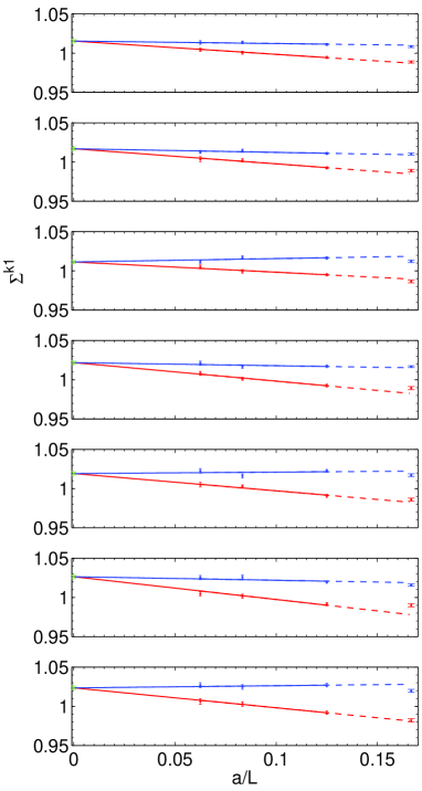
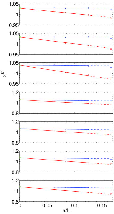
Figure 10: Continuum limit extrapolations of the $N_{\mathrm{\scriptstyle f}}=0$ SSF for the renormalization scheme $\alpha=1/2$. Blue (red) points correspond to results with the $\mbox{O}(a)$ improved (unimproved) action, respectively.

	$\alpha=0$		$\alpha=1/2$
$u$	$\sigma_{\rm\scriptscriptstyle T}(u)$	$\chi^{2}/{\rm dof}$	$\sigma_{\rm\scriptscriptstyle T}(u)$	$\chi^{2}/{\rm dof}$
0.8873	1.0168(31)	0.23	1.0155(27)	0.20
0.9944	1.0190(34)	0.46	1.0171(30)	0.41
1.0989	1.0127(34)	0.69	1.0115(30)	1.18
1.2430	1.0242(38)	0.61	1.0219(33)	0.54
1.3293	1.0215(42)	1.49	1.0192(36)	1.83
1.4300	1.0295(42)	1.48	1.0265(36)	1.52
1.5553	1.0268(51)	0.20	1.0235(43)	0.20
1.6950	1.0347(50)	0.64	1.0294(42)	0.60
1.8811	1.0380(53)	1.01	1.0320(45)	1.03
2.1000	1.0461(50)	0.58	1.0381(40)	1.08
2.4484	1.0688(57)	3.41	1.0550(45)	3.65
2.7700	1.0912(63)	0.06	1.0677(50)	0.05
3.1110	1.1001(67)	1.00	1.0738(51)	0.86
3.4800	1.1128(76)	1.00	1.0806(57)	1.09

Table 6: Continuum-extrapolated values for the SSFs for $N_{\mathrm{\scriptstyle f}}=0$.

	fit	$p_{1}$	$p_{2}$	$p_{3}$	$p_{4}$	$\chi^{2}/{\rm dof}$
$\alpha=0$	A	0.011705	0.00611(32)	—	—	1.16
	B	0.011705	0.0042(12)	0.00072(45)	—	1.04
	C	0.011705	0.005449	0.00028(11)	—	1.04
	D	0.011705	0.005449	-0.00005(66)	0.00011(22)	1.11
	E	0.011705	-0.0006(37)	0.0051(32)	-0.00089(64)	0.96
$\alpha=1/2$	A	0.011705	0.00370(25)	—	—	0.88
	B	0.011705	0.0035(10)	0.000072(36)	—	0.95
	C	0.011705	0.005043	-0.000455(88)	—	1.05
	D	0.011705	0.005043	-0.00098(54)	0.00017(17)	1.06
	E	0.011705	-0.0003(31)	0.0034(26)	-0.00068(52)	0.88

Table 7: Fits to the continuum $N_{\mathrm{\scriptstyle f}}=0$ SSFs for various choices of polynomial ansatz, cf. Eq. (5.53).

k	$u_{k}$	$[U(\mu_{\rm\scriptscriptstyle had},2^{k+1}\mu_{\rm\scriptscriptstyle had})]^{-1}$	$\hat{c}^{1/2}(\mu_{\rm\scriptscriptstyle had})$	$\hat{c}^{2/2}(\mu_{\rm\scriptscriptstyle had})$	$\mathbf{\hat{c}^{2/3}(\boldsymbol{\mu}_{\rm\scriptscriptstyle\bf had})}$	$\hat{c}^{3/3}(\mu_{\rm\scriptscriptstyle had})$
0	3.480	0.8916(45)	1.0655(53)	0.9099(45)	0.9133(46)	0.8201(41)
1	2.455(18)	0.8376(51)	1.0377(64)	0.9256(59)	0.9272(59)	0.8768(59)
2	1.918(15)	0.8031(54)	1.0218(70)	0.9332(66)	0.9342(66)	0.9021(65)
3	1.584(13)	0.7783(57)	1.0113(76)	0.9378(72)	0.9384(72)	0.9160(72)
4	1.353(13)	0.7592(60)	1.0039(82)	0.9408(78)	0.9412(78)	0.9246(78)
5	1.184(12)	0.7436(63)	0.9983(87)	0.9429(84)	0.9433(84)	0.9304(84)
6	1.053(12)	0.7306(66)	0.9939(93)	0.9446(90)	0.9448(90)	0.9346(90)
7	0.950(11)	0.7195(68)	0.9905(98)	0.9459(95)	0.9461(95)	0.9377(95)
8	0.865(10)	0.7097(70)	0.9876(102)	0.9469(99)	0.9471(99)	0.9401(99)

Table 8: Non-perturbative $N_{\mathrm{\scriptstyle f}}=0$ running in the scheme $\alpha=0$. (Our best result $\hat{c}^{2/3}(\mu_{\rm\scriptscriptstyle had})$ is stressed.)

k	$u_{k}$	$[U(\mu_{\rm\scriptscriptstyle had},2^{k+1}\mu_{\rm\scriptscriptstyle had})]^{-1}$	$\hat{c}^{1/2}(\mu_{\rm\scriptscriptstyle had})$	$\hat{c}^{2/2}(\mu_{\rm\scriptscriptstyle had})$	$\mathbf{\hat{c}^{2/3}(\boldsymbol{\mu}_{\rm\scriptscriptstyle\bf had})}$	$\hat{c}^{3/3}(\mu_{\rm\scriptscriptstyle had})$
0	3.480	0.9207(36)	1.1003(44)	0.9522(38)	0.9556(38)	0.8732(35)
1	2.455(18)	0.8762(41)	1.0855(52)	0.9776(49)	0.9792(49)	0.9344(49)
2	1.918(15)	0.8459(44)	1.0761(57)	0.9904(54)	0.9914(54)	0.9628(54)
3	1.584(13)	0.8231(47)	1.0695(63)	0.9981(60)	0.9987(60)	0.9787(60)
4	1.353(13)	0.8051(50)	1.0646(69)	1.0031(66)	1.0036(66)	0.9888(66)
5	1.184(12)	0.7902(54)	1.0608(74)	1.0068(72)	1.0071(72)	0.9956(72)
6	1.053(12)	0.7775(57)	1.0577(80)	1.0095(78)	1.0098(78)	1.0006(78)
7	0.950(11)	0.7665(59)	1.0552(85)	1.0116(83)	1.0119(83)	1.0043(83)
8	0.865(10)	0.7568(62)	1.0531(89)	1.0133(87)	1.0135(87)	1.0072(87)

Table 9: Non-perturbative $N_{\mathrm{\scriptstyle f}}=0$ running in the scheme $\alpha=1/2$. (Our best result $\hat{c}^{2/3}(\mu_{\rm\scriptscriptstyle had})$ is stressed.)

		$c_{\rm sw}={\rm NP}$		$c_{\rm sw}=0$
$\beta$	$\frac{L}{a}$	$\qquad\kappa_{\rm c}$	$\,\,\quad Z_{\rm\scriptscriptstyle T}$	$\qquad\kappa_{\rm c}$	$\,\,\quad Z_{\rm\scriptscriptstyle T}$
6.0219	8	0.135043(17)	1.0401(21)	0.153371(10)	0.9407(19)
6.1628	10	0.135643(11)	1.0606(13)	0.152012(7)	0.9617(16)
6.2885	12	0.135739(13)	1.0738(15)	0.150752(10)	0.9792(24)
6.4956	16	0.135577(7)	1.0950(35)	0.148876(13)	1.0022(35)

Table 10: Renormalization constants $Z_{\rm\scriptscriptstyle T}(g_{0}^{2},L/a)$ at $L=1/\mu_{\rm\scriptscriptstyle had}$ for $N_{\mathrm{\scriptstyle f}}=0$, scheme $\alpha=0$.

		$c_{\rm sw}={\rm NP}$		$c_{\rm sw}=0$
$\beta$	$\frac{L}{a}$	$\qquad\kappa_{\rm c}$	$\,\,\quad Z_{\rm\scriptscriptstyle T}$	$\qquad\kappa_{\rm c}$	$\,\,\quad Z_{\rm\scriptscriptstyle T}$
6.0219	8	0.135043(17)	0.9715(15)	0.153371(10)	0.8853(15)
6.1628	10	0.135643(11)	0.9909(9)	0.152012(7)	0.9033(13)
6.2885	12	0.135739(13)	1.0044(11)	0.150752(10)	0.9178(18)
6.4956	16	0.135577(7)	1.0236(24)	0.148876(13)	0.9399(27)

Table 11: Renormalization constants $Z_{\rm\scriptscriptstyle T}(g_{0}^{2},L/a)$ at $L=1/\mu_{\rm\scriptscriptstyle had}$ for $N_{\mathrm{\scriptstyle f}}=0$, scheme $\alpha=1/2$.

	$c_{\rm sw}={\rm NP}$		$c_{\rm sw}=0$
$\beta$	$\hat{Z}_{\rm\scriptscriptstyle T}^{\alpha=0}$	$\hat{Z}_{\rm\scriptscriptstyle T}^{\alpha=1/2}$	$\hat{Z}_{\rm\scriptscriptstyle T}^{\alpha=0}$	$\hat{Z}_{\rm\scriptscriptstyle T}^{\alpha=1/2}$
6.0129	0.984(10)	0.983(8)	0.890(9)	0.896(8)
6.1628	1.003(10)	1.003(8)	0.910(9)	0.914(8)
6.2885	1.016(10)	1.016(8)	0.926(10)	0.929(8)
6.4956	1.036(11)	1.036(9)	0.948(10)	0.951(8)

Table 12: RGI renormalization factors $\hat{Z}_{\rm\scriptscriptstyle T}$ for $N_{\mathrm{\scriptstyle f}}=0$.

				$\alpha=0$			$\alpha=1/2$
$\kern 1.0pt\overline{\kern-1.0ptg\kern 0.0pt}\kern 1.0pt^{2}_{\rm\scriptscriptstyle SF}(L)$	$\beta$	$\kappa_{\rm c}$	$L/a$	$Z_{\rm\scriptscriptstyle T}(g_{0}^{2},L/a)$	$Z_{\rm\scriptscriptstyle T}(g_{0}^{2},2L/a)$	$\Sigma_{\rm\scriptscriptstyle T}(g_{0}^{2},L/a)$	$Z_{\rm\scriptscriptstyle T}(g_{0}^{2},L/a)$	$Z_{\rm\scriptscriptstyle T}(g_{0}^{2},2L/a)$	$\Sigma_{\rm\scriptscriptstyle T}(g_{0}^{2},L/a)$
0.9793	9.50000	0.131532	6	0.97814(88)	0.9895(14)	1.0116(17)	0.96579(74)	0.9778(11)	1.0124(14)
	9.73410	0.131305	8	0.98014(87)	0.9914(20)	1.0115(22)	0.96924(76)	0.9806(17)	1.0118(19)
	10.05755	0.131069	12	0.98792(92)	1.0062(25)	1.0185(27)	0.97789(79)	0.9947(23)	1.0172(25)
1.1814	8.50000	0.132509	6	0.97574(94)	0.9902(39)	1.0148(42)	0.95998(79)	0.9755(33)	1.0161(35)
	8.72230	0.132291	8	0.9819(17)	1.0032(15)	1.0217(24)	0.9674(15)	0.9881(13)	1.0214(21)
	8.99366	0.131975	12	0.9902(11)	1.0135(37)	1.0236(39)	0.97665(91)	0.9987(32)	1.0226(35)
1.5078	7.54200	0.133705	6	0.97715(94)	1.0019(30)	1.0253(32)	0.95543(79)	0.9792(24)	1.0249(26)
	7.72060	0.133497	8	0.9830(22)	1.0131(39)	1.0306(46)	0.9631(18)	0.9909(33)	1.0289(39)
1.5031	7.50000	0.133815	6	0.97702(84)	0.9931(35)	1.0164(37)	0.95515(71)	0.9721(29)	1.0177(31)
	8.02599	0.133063	12	0.9925(23)	1.01982(58)	1.0275(25)	0.9743(21)	0.9988(29)	1.0252(37)
2.0142	6.60850	0.135260	6	0.9808(13)	1.0158(22)	1.0357(26)	0.9484(10)	0.9808(17)	1.0342(21)
	6.82170	0.134891	8	0.9879(22)	1.0311(26)	1.0438(35)	0.9592(18)	0.9966(22)	1.0390(30)
	7.09300	0.134432	12	1.0042(23)	1.0433(13)	1.0389(27)	0.9770(18)	1.0112(10)	1.0351(22)
2.4792	6.13300	0.136110	6	0.9890(21)	1.0407(70)	1.0523(74)	0.9460(17)	0.9916(56)	1.0483(62)
	6.32290	0.135767	8	0.9952(14)	1.0435(84)	1.0485(86)	0.9568(11)	0.9981(66)	1.0431(70)
	6.63164	0.135227	12	1.0123(32)	1.0756(13)	1.0625(36)	0.9787(24)	1.03073(99)	1.0531(28)
3.3340	5.62150	0.136665	6	1.0024(38)	1.080(15)	1.077(16)	0.9405(29)	0.9993(92)	1.062(10)
	5.80970	0.136608	8	1.0171(39)	1.129(12)	1.110(13)	0.9608(27)	1.0402(95)	1.083(10)
	6.11816	0.136139	12	1.0335(56)	1.126(12)	1.090(13)	0.9844(41)	1.0479(67)	1.0645(81)

Table 13: $N_{\mathrm{\scriptstyle f}}=2$ results for the renormalization constant $Z_{\rm\scriptscriptstyle T}$ and the step scaling function $\Sigma_{\rm\scriptscriptstyle T}$.

figureContinuum extrapolations of SSFs for $N_{\mathrm{\scriptstyle f}}=2$ in the schemes $\alpha=0$ (left) and $\alpha=1/2$ (right). Blue points are the data in Table 13; red points result from subtracting the one-loop value of cutoff effects.

	$\alpha=0$			$\alpha=1/2$
$u$	$\sigma_{\rm\scriptscriptstyle T}$	$\rho(u)$	$\chi^{2}/{\rm dof}$	$\sigma_{\rm\scriptscriptstyle T}$	$\rho(u)$	$\chi^{2}/{\rm dof}$
0.9793	1.0179(32)	-0.25(14)	2.22	1.0163(28)	-0.15(13)	1.87
1.1814	1.0278(48)	-0.43(27)	0.22	1.0258(41)	-0.32(23)	0.21
1.5078	1.0317(34)	-0.21(11)	0.28	1.0291(44)	-0.13(12)	0.35
		-0.55(20)			-0.41(19)
2.0142	1.0419(35)	-0.18(18)	2.37	1.0365(28)	-0.06(14)	1.61
2.4792	1.0656(54)	-0.57(39)	1.08	1.0546(42)	-0.31(32)	1.09
3.3340	1.103(17)	-0.57(96)	2.59	1.070(11)	-0.06(63)	2.42

Table 14: $N_{\mathrm{\scriptstyle f}}=2$ continuum-extrapolated values of $\sigma_{\rm\scriptscriptstyle T}$ without subtraction of perturbative cutoff effects. The two lines for $u=1.5078$ correspond to the use of the one- and two-loop value of $c_{\rm t}$, respectively.

	$\alpha=0$			$\alpha=1/2$
$u$	$\sigma_{\rm\scriptscriptstyle T}(u)$	$\rho(u)$	$\chi^{2}/{\rm dof}$	$\sigma_{\rm\scriptscriptstyle T}(u)$	$\rho(u)$	$\chi^{2}/{\rm dof}$
0.9793	1.0178(32)	-0.04(14)	2.05	1.0159(28)	0.03(13)	1.78
1.1814	1.0276(48)	-0.17(27)	0.27	1.0254(41)	-0.09(24)	0.24
1.5078	1.0315(34)	0.13(12)	0.33	1.0285(44)	0.16(12)	0.376
		-0.22(20)			-0.12(19)
2.0142	1.0415(35)	0.28(18)	2.63	1.0356(28)	0.34(14)	1.73
2.4792	1.0651(55)	0.01(39)	0.99	1.0535(43)	0.19(32)	1.04
3.3340	1.102(17)	0.25(97)	2.70	1.068(11)	0.63(64)	2.49

Table 15: $N_{\mathrm{\scriptstyle f}}=2$ continuum-extrapolated values of $\sigma_{\rm\scriptscriptstyle T}$ with subtraction of perturbative cutoff effects. The two lines for $u=1.5078$ correspond to the use of the one- and two-loop value of $c_{\rm t}$, respectively.

	fit	$p_{1}$	$p_{2}$	$p_{3}$	$p_{4}$	$\chi^{2}/{\rm dof}$
$\alpha=0$	A	0.011705	0.0055(5)	-	-	0.73
	B	0.011705	0.0059(22)	-0.00018(94)	-	0.90
	C	0.011705	0.005070	0.00015(23)	-	0.75
	D	0.011705	0.005070	0.00016(10)	-0.0000(4)	0.93
	E	0.011705	0.0116(62)	-0.0055(55)	0.0012(12)	0.87
$\alpha=1/2$	A	0.011705	0.00351(42)	-	-	1.00
	B	0.011705	0.0054(18)	-0.00080(74)	-	0.96
	C	0.011705	0.004713	-0.00053(17)	-	0.80
	D	0.011705	0.004713	-0.00034(83)	-0.00007(31)	0.98
	E	0.011705	0.0076(55)	-0.0027(46)	0.00040(95)	1.22

Table 16: Fits to the continuum $N_{\mathrm{\scriptstyle f}}=2$ SSFs for various choices of polynomial ansatz, cf. Eq. (5.53).

k	$u_{k}$	$[U(\mu_{\rm\scriptscriptstyle had},2^{k+1}\mu_{\rm\scriptscriptstyle had})]^{-1}$	$\hat{c}^{1/2}(\mu_{\rm\scriptscriptstyle had})$	$\hat{c}^{2/2}(\mu_{\rm\scriptscriptstyle had})$	$\mathbf{\hat{c}^{2/3}(\boldsymbol{\mu}_{\rm\scriptscriptstyle\bf had})}$	$\hat{c}^{3/3}(\mu_{\rm\scriptscriptstyle had})$
-1	4.610	1	1.1818	0.9483	0.9495	0.7871
0	3.032(16)	0.922(7)	1.144(9)	0.985(8)	0.986(8)	0.905(7)
1	2.341(21)	0.872(8)	1.117(11)	0.993(10)	0.993(10)	0.943(10)
2	1.918(20)	0.837(9)	1.098(12)	0.996(11)	0.996(11)	0.962(11)
3	1.628(17)	0.809(9)	1.084(13)	0.998(12)	0.998(12)	0.973(12)
4	1.414(14)	0.787(9)	1.074(13)	0.999(12)	0.999(12)	0.980(12)
5	1.251(12)	0.769(9)	1.067(14)	1.000(13)	1.000(13)	0.985(13)
6	1.121(11)	0.754(10)	1.060(14)	1.001(14)	1.001(14)	0.988(13)
7	1.017(10)	0.741(10)	1.055(15)	1.001(14)	1.001(14)	0.991(14)

Table 17: Non-perturbative $N_{\mathrm{\scriptstyle f}}=2$ running in the scheme $\alpha=0$. (Our best result $\hat{c}^{2/3}(\mu_{\rm\scriptscriptstyle had})$ is stressed.)

k	$u_{k}$	$[U(\mu_{\rm\scriptscriptstyle had},2^{k+1}\mu_{\rm\scriptscriptstyle had})]^{-1}$	$\hat{c}^{1/2}(\mu_{\rm\scriptscriptstyle had})$	$\hat{c}^{2/2}(\mu_{\rm\scriptscriptstyle had})$	$\mathbf{\hat{c}^{2/3}(\boldsymbol{\mu}_{\rm\scriptscriptstyle\bf had})}$	$\hat{c}^{3/3}(\mu_{\rm\scriptscriptstyle had})$
-1	4.610	1	1.1818	0.9650	0.9661	0.8241
0	3.032(16)	0.941(5)	1.167(7)	1.017(6)	1.018(6)	0.947(6)
1	2.341(21)	0.899(7)	1.151(9)	1.033(8)	1.033(8)	0.989(8)
2	1.918(20)	0.867(7)	1.138(10)	1.041(9)	1.041(9)	1.010(9)
3	1.628(17)	0.842(7)	1.128(10)	1.045(10)	1.045(10)	1.023(10)
4	1.414(14)	0.821(8)	1.121(11)	1.048(10)	1.048(10)	1.031(10)
5	1.251(12)	0.804(8)	1.115(12)	1.051(11)	1.051(11)	1.037(11)
6	1.121(11)	0.789(8)	1.110(12)	1.052(12)	1.052(12)	1.041(12)
7	1.017(10)	0.776(9)	1.106(13)	1.053(12)	1.053(12)	1.044(12)

Table 18: Non-perturbative $N_{\mathrm{\scriptstyle f}}=2$ running in the scheme $\alpha=1/2$. (Our best result $\hat{c}^{2/3}(\mu_{\rm\scriptscriptstyle had})$ is stressed.)

$\beta$	$\kappa_{\rm c}$	$L/a$	$\bar{g}^{2}_{\rm\scriptscriptstyle SF}(L)$	$Z_{\rm\scriptscriptstyle T}^{\alpha=0}$	$Z_{\rm\scriptscriptstyle T}^{\alpha=1/2}$
5.20	0.13600	4	3.65(3)	1.0256(13)	0.9263(10)
		6	4.61(4)	1.0678(17)	0.9608(11)
5.29	0.13641	4	3.394(17)	1.0133(12)	0.9251(9)
		6	4.297(37)	1.0487(20)	0.9556(14)
		8	5.65(9)	1.0958(22)	0.9886(15)
5.40	0.13669	4	3.188(24)	1.0054(11)	0.9270(9)
		6	3.864(34)	1.0306(16)	0.9500(12)
		8	4.747(63)	1.0671(17)	0.9781(12)

Table 19: Renormalization constants $Z_{\rm\scriptscriptstyle T}(g_{0}^{2},L/a)$ at $L=1/\mu_{\rm\scriptscriptstyle had}$ for $N_{\mathrm{\scriptstyle f}}=2$.

$\beta$	$\hat{Z}_{\rm\scriptscriptstyle T}^{\alpha=0}$	$\hat{Z}_{\rm\scriptscriptstyle T}^{\alpha=1/2}$
5.20	1.069(15)	1.012(12)
5.29	1.060(15)	1.012(12)
5.40	1.062(15)	1.026(12)

Table 20: RGI renormalization factors $\hat{Z}_{\rm\scriptscriptstyle T}$ for $N_{\mathrm{\scriptstyle f}}=2$.

References

- [1] M. Artuso et al., , and decays, Eur. Phys. J. C57 (2008) 309–492, [0801.1833].
- [2] M. Antonelli et al., Flavor Physics in the Quark Sector, Phys. Rept. 494 (2010) 197–414, [0907.5386].
- [3] T. Blake, G. Lanfranchi and D. M. Straub, Rare Decays as Tests of the Standard Model, Prog. Part. Nucl. Phys. 92 (2017) 50–91, [1606.00916].
- [4] T. Bhattacharya, V. Cirigliano, R. Gupta, H.-W. Lin and B. Yoon, Neutron Electric Dipole Moment and Tensor Charges from Lattice QCD, Phys. Rev. Lett. 115 (2015) 212002, [1506.04196].
- [5] T. Bhattacharya, V. Cirigliano, S. Cohen, R. Gupta, H.-W. Lin and B. Yoon, Axial, Scalar and Tensor Charges of the Nucleon from 2+1+1-flavor Lattice QCD, Phys. Rev. D94 (2016) 054508, [1606.07049].
- [6] M. Abramczyk, S. Aoki, T. Blum, T. Izubuchi, H. Ohki and S. Syritsyn, On Lattice Calculation of Electric Dipole Moments and Form Factors of the Nucleon, 1701.07792.
- [7] S. Capitani, M. Lüscher, R. Sommer and H. Wittig, Non-perturbative quark mass renormalization in quenched lattice QCD, Nucl. Phys. B544 (1999) 669–698, [hep-lat/9810063]. [Erratum: Nucl. Phys.B582,762(2000)].
- [8] ALPHA collaboration, M. Della Morte, R. Hoffmann, F. Knechtli, J. Rolf, R. Sommer, I. Wetzorke et al., Non-perturbative quark mass renormalization in two-flavor QCD, Nucl. Phys. B729 (2005) 117–134, [hep-lat/0507035].
- [9] I. Campos, P. Fritzsch, C. Pena, D. Preti, A. Ramos and A. Vladikas, Non-perturbative running of quark masses in three-flavour QCD, PoS LATTICE2016 (2016) 201, [1611.09711].
- [10] I. Campos, P. Fritzsch, C. Pena, D. Preti, A. Ramos and A. Vladikas, Controlling quark mass determinations non-perturbatively in three-flavour QCD, EPJ Web Conf. 137 (2017) 08006, [1611.06102].
- [11] J. A. Gracey, Three loop MS-bar tensor current anomalous dimension in QCD, Phys. Lett. B488 (2000) 175–181, [hep-ph/0007171].
- [12] L. G. Almeida and C. Sturm, Two-loop matching factors for light quark masses and three-loop mass anomalous dimensions in the RI/SMOM schemes, Phys. Rev. D82 (2010) 054017, [1004.4613].
- [13] A. Skouroupathis and H. Panagopoulos, Two-loop renormalization of vector, axial-vector and tensor fermion bilinears on the lattice, Phys. Rev. D79 (2009) 094508, [0811.4264].
- [14] M. Göckeler, R. Horsley, H. Oelrich, H. Perlt, D. Petters, P. E. L. Rakow et al., Nonperturbative renormalization of composite operators in lattice QCD, Nucl. Phys. B544 (1999) 699–733, [hep-lat/9807044].
- [15] D. Bečirević, V. Giménez, V. Lubicz, G. Martinelli, M. Papinutto and J. Reyes, Renormalization constants of quark operators for the nonperturbatively improved Wilson action, JHEP 08 (2004) 022, [hep-lat/0401033].
- [16] Y. Aoki et al., Non-perturbative renormalization of quark bilinear operators and B(K) using domain wall fermions, Phys. Rev. D78 (2008) 054510, [0712.1061].
- [17] C. Sturm, Y. Aoki, N. H. Christ, T. Izubuchi, C. T. C. Sachrajda and A. Soni, Renormalization of quark bilinear operators in a momentum-subtraction scheme with a nonexceptional subtraction point, Phys. Rev. D80 (2009) 014501, [0901.2599].
- [18] ETM collaboration, M. Constantinou et al., Non-perturbative renormalization of quark bilinear operators with (tmQCD) Wilson fermions and the tree-level improved gauge action, JHEP 08 (2010) 068, [1004.1115].
- [19] C. Alexandrou, M. Constantinou, T. Korzec, H. Panagopoulos and F. Stylianou, Renormalization constants of local operators for Wilson type improved fermions, Phys. Rev. D86 (2012) 014505, [1201.5025].
- [20] M. Constantinou, R. Horsley, H. Panagopoulos, H. Perlt, P. E. L. Rakow, G. Schierholz et al., Renormalization of local quark-bilinear operators for =3 flavors of stout link nonperturbative clover fermions, Phys. Rev. D91 (2015) 014502, [1408.6047].
- [21] M. Lüscher, R. Narayanan, P. Weisz and U. Wolff, The Schrodinger functional: A Renormalizable probe for nonAbelian gauge theories, Nucl. Phys. B384 (1992) 168–228, [hep-lat/9207009].
- [22] I. Campos, P. Fritzsch, C. Pena, D. Preti, A. Ramos and A. Vladikas, Non-perturbative renormalization of quark masses in three-flavour QCD, .
- [23] B. Blossier, M. della Morte, N. Garron and R. Sommer, HQET at order : I. Non-perturbative parameters in the quenched approximation, JHEP 06 (2010) 002, [1001.4783].
- [24] ALPHA collaboration, F. Bernardoni et al., Decay constants of B-mesons from non-perturbative HQET with two light dynamical quarks, Phys. Lett. B735 (2014) 349–356, [1404.3590].
- [25] ALPHA collaboration, M. Guagnelli, J. Heitger, C. Pena, S. Sint and A. Vladikas, Non-perturbative renormalization of left-left four-fermion operators in quenched lattice QCD, JHEP 03 (2006) 088, [hep-lat/0505002].
- [26] F. Palombi, C. Pena and S. Sint, A Perturbative study of two four-quark operators in finite volume renormalization schemes, JHEP 03 (2006) 089, [hep-lat/0505003].
- [27] P. Dimopoulos, L. Giusti, P. Hernández, F. Palombi, C. Pena, A. Vladikas et al., Non-perturbative renormalisation of left-left four-fermion operators with Neuberger fermions, Phys. Lett. B641 (2006) 118–124, [hep-lat/0607028].
- [28] ALPHA collaboration, P. Dimopoulos, G. Herdoíza, F. Palombi, M. Papinutto, C. Pena, A. Vladikas et al., Non-perturbative renormalisation of Delta F=2 four-fermion operators in two-flavour QCD, JHEP 05 (2008) 065, [0712.2429].
- [29] F. Palombi, M. Papinutto, C. Pena and H. Wittig, Non-perturbative renormalization of static-light four-fermion operators in quenched lattice QCD, JHEP 09 (2007) 062, [0706.4153].
- [30] M. Papinutto, C. Pena and D. Preti, Non-perturbative renormalization and running of Delta F=2 four-fermion operators in the SF scheme, PoS LATTICE2014 (2014) 281, [1412.1742].
- [31] M. Papinutto, C. Pena and D. Preti, On the perturbative renormalisation of four-quark operators for new physics, 1612.06461.
- [32] P. Fritzsch, C. Pena and D. Preti, Non-perturbative renormalization of tensor bilinears in Schrödinger Functional schemes, PoS LATTICE2015 (2016) 250, [1511.05024].
- [33] M. Dalla Brida, S. Sint and P. Vilaseca, The chirally rotated Schrödinger functional: theoretical expectations and perturbative tests, JHEP 08 (2016) 102, [1603.00046].
- [34] ALPHA collaboration, M. Dalla Brida, P. Fritzsch, T. Korzec, A. Ramos, S. Sint and R. Sommer, Determination of the QCD -parameter and the accuracy of perturbation theory at high energies, Phys. Rev. Lett. 117 (2016) 182001, [1604.06193].
- [35] ALPHA collaboration, M. Dalla Brida, P. Fritzsch, T. Korzec, A. Ramos, S. Sint and R. Sommer, Slow running of the Gradient Flow coupling from 200 MeV to 4 GeV in QCD, Phys. Rev. D95 (2017) 014507, [1607.06423].
- [36] M. Bruno, M. Dalla Brida, P. Fritzsch, T. Korzec, A. Ramos, S. Schaefer et al., The strong coupling from a nonperturbative determination of the parameter in three-flavor QCD, 1706.03821.
- [37] P. Fritzsch, C. Pena and D. Preti, Non-perturbative renormalization of tensor currents in three-flavour QCD, .
- [38] G. ’t Hooft, Dimensional regularization and the renormalization group, Nucl. Phys. B61 (1973) 455–468.
- [39] W. A. Bardeen, A. J. Buras, D. W. Duke and T. Muta, Deep Inelastic Scattering Beyond the Leading Order in Asymptotically Free Gauge Theories, Phys. Rev. D18 (1978) 3998.
- [40] G. Martinelli, C. Pittori, C. T. Sachrajda, M. Testa and A. Vladikas, A General method for nonperturbative renormalization of lattice operators, Nucl. Phys. B445 (1995) 81–108, [hep-lat/9411010].
- [41] K. Jansen, C. Liu, M. Lüscher, H. Simma, S. Sint, R. Sommer et al., Nonperturbative renormalization of lattice QCD at all scales, Phys. Lett. B372 (1996) 275–282, [hep-lat/9512009].
- [42] V. S. Vanyashin and M. V. Terent’ev, The vacuum polarization of a charged vector field, JETP 21 (1965) 375.
- [43] I. B. Khriplovich, Green’s functions in theories with non-abelian gauge group., Sov. J. Nucl. Phys. 10 (1969) 235–242. [Yad. Fiz.10,409(1969)].
- [44] G. ’t Hooft , report at the Colloquium on Renormalization of Yang-Mills Fields and Applications to Particle Physics, Marseille, France, June 1972 (unpublished).
- [45] D. J. Gross and F. Wilczek, Ultraviolet Behavior of Nonabelian Gauge Theories, Phys. Rev. Lett. 30 (1973) 1343–1346.
- [46] H. D. Politzer, Reliable Perturbative Results for Strong Interactions?, Phys. Rev. Lett. 30 (1973) 1346–1349.
- [47] W. E. Caswell, Asymptotic Behavior of Nonabelian Gauge Theories to Two Loop Order, Phys. Rev. Lett. 33 (1974) 244.
- [48] D. R. T. Jones, Two Loop Diagrams in Yang-Mills Theory, Nucl. Phys. B75 (1974) 531.
- [49] J. Gasser and H. Leutwyler, Quark Masses, Phys. Rept. 87 (1982) 77–169.
- [50] J. Gasser and H. Leutwyler, Chiral Perturbation Theory to One Loop, Annals Phys. 158 (1984) 142.
- [51] J. Gasser and H. Leutwyler, Chiral Perturbation Theory: Expansions in the Mass of the Strange Quark, Nucl. Phys. B250 (1985) 465–516.
- [52] M. Lüscher, S. Sint, R. Sommer and P. Weisz, Chiral symmetry and O(a) improvement in lattice QCD, Nucl. Phys. B478 (1996) 365–400, [hep-lat/9605038].
- [53] S. Capitani, M. Guagnelli, M. Lüscher, S. Sint, R. Sommer, P. Weisz et al., Nonperturbative quark mass renormalization, Nucl. Phys. Proc. Suppl. 63 (1998) 153–158, [hep-lat/9709125].
- [54] ALPHA collaboration, S. Sint and P. Weisz, The Running quark mass in the SF scheme and its two loop anomalous dimension, Nucl. Phys. B545 (1999) 529–542, [hep-lat/9808013].
- [55] I. Campos, P. Fritzsch, C. Pena, D. Preti, A. Ramos and A. Vladikas, Prospects and status of quark mass renormalization in three-flavour QCD, PoS LATTICE2015 (2016) 249, [1508.06939].
- [56] M. Guagnelli, K. Jansen and R. Petronzio, Nonperturbative running of the average momentum of nonsinglet parton densities, Nucl. Phys. B542 (1999) 395–409, [hep-lat/9809009].
- [57] M. Guagnelli, K. Jansen and R. Petronzio, Renormalization group invariant average momentum of nonsinglet parton densities, Phys. Lett. B459 (1999) 594–598, [hep-lat/9903012].
- [58] ZeRo collaboration, A. Shindler, M. Guagnelli, K. Jansen, F. Palombi, R. Petronzio and I. Wetzorke, Nonperturbative renormalization of moments of parton distribution functions, Nucl. Phys. Proc. Suppl. 129 (2004) 278–280, [hep-lat/0309181].
- [59] C. Pica, Beyond the Standard Model: Charting Fundamental Interactions via Lattice Simulations, PoS LATTICE2016 (2016) 015, [1701.07782].
- [60] S. Sint , unpublished notes, 1996.
- [61] S. Sint and P. Weisz, Further one loop results in improved lattice QCD, Nucl. Phys. Proc. Suppl. 63 (1998) 856–858, [hep-lat/9709096].
- [62] M. Lüscher, R. Sommer, P. Weisz and U. Wolff, A Precise determination of the running coupling in the SU(3) Yang-Mills theory, Nucl. Phys. B413 (1994) 481–502, [hep-lat/9309005].
- [63] S. Sint and R. Sommer, The Running coupling from the QCD Schrodinger functional: A One loop analysis, Nucl. Phys. B465 (1996) 71–98, [hep-lat/9508012].
- [64] S. Capitani, M. Göckeler, R. Horsley, H. Perlt, P. E. L. Rakow, G. Schierholz et al., Renormalization and off-shell improvement in lattice perturbation theory, Nucl. Phys. B593 (2001) 183–228, [hep-lat/0007004].
- [65] J. A. Gracey, Three loop anomalous dimension of the second moment of the transversity operator in the MS-bar and RI-prime schemes, Nucl. Phys. B667 (2003) 242–260, [hep-ph/0306163].
- [66] ALPHA collaboration, M. Della Morte, R. Frezzotti, J. Heitger, J. Rolf, R. Sommer and U. Wolff, Computation of the strong coupling in QCD with two dynamical flavors, Nucl. Phys. B713 (2005) 378–406, [hep-lat/0411025].
- [67] R. Sommer, A New way to set the energy scale in lattice gauge theories and its applications to the static force and in SU(2) Yang-Mills theory, Nucl. Phys. B411 (1994) 839–854, [hep-lat/9310022].
- [68] ALPHA collaboration, K. Jansen and R. Sommer, O() improvement of lattice QCD with two flavors of Wilson quarks, Nucl. Phys. B530 (1998) 185–203, [hep-lat/9803017]. [Erratum: Nucl. Phys.B643,517(2002)].
- [69] ALPHA collaboration, A. Bode, P. Weisz and U. Wolff, Two loop computation of the Schrodinger functional in lattice QCD, Nucl. Phys. B576 (2000) 517–539, [hep-lat/9911018]. [Erratum: Nucl. Phys.B600,453(2001)].
- [70] ALPHA collaboration, U. Wolff, Monte Carlo errors with less errors, Comput. Phys. Commun. 156 (2004) 143–153, [hep-lat/0306017]. [Erratum: Comput. Phys. Commun.176,383(2007)].
- [71] S. Sint and P. Weisz, Further results on improved lattice QCD to one loop order of perturbation theory, Nucl. Phys. B502 (1997) 251–268, [hep-lat/9704001].