Click-aware Purchase Prediction with Push at the Top

Abstract

Eliciting user preferences from purchase records for the task of purchase prediction is challenging because negative feedback is not explicitly observed, and treating all the non-purchased items equally as negative feedback is unrealistic. In this paper, we present a framework that leverages users’ past click records to complement the missing user–item interactions of purchase records, i.e., non-purchased items. We begin by formulating various model assumptions, each assuming a different order of user preferences among purchased, clicked-but-not-purchased and non-clicked items, to study the usefulness of leveraging click records. We implement the model assumptions under the Bayesian Personalized Ranking model, which maximizes the Area Under the Curve (AUC) for bipartite ranking. However, we argue that using click records for bipartite ranking needs a meticulously designed model owing to the relative unreliableness of click records compared with purchase records. To address this issue, we ultimately propose a novel learning-to-rank method for purchase prediction, called P3STop, that is customized to be robust to relatively unreliable click records by particularly focusing on the accuracy of the top-ranked items. Experimental results on two real-world e-commerce datasets demonstrate that P3STop considerably outperforms the state-of-the-art implicit feedback–based recommendation methods, especially for the top-ranked items.

1 Introduction

Implicit feedback, such as purchases and clicks, are easily obtained from system logs, but precisely eliciting users’ preferences from implicit feedback for purchase prediction is challenging because negative feedback is not explicitly observed. In this respect, past research has focused on inferring users’ negative feedback from missing user–item interactions. Specifically, a uniform weighting scheme [15, 41] in which all missing data are treated as negative feedback (i.e., All Missing As Negative (AMAN) assumption) has been introduced. However, this assumption is not entirely valid in that the reason why items are not observed is uncertain; whether a user does not like them or a user is simply not aware of them. To cope with the drawback of the AMAN assumption, sampling–based approaches such as user-oriented sampling [33] or item-popularity-oriented sampling [11, 40] have been proposed. However, the sampling–based approaches are essentially based on predefined heuristic weights [3] that are not guaranteed to always hold in the real data.

In this paper, we present a framework that leverages users’ past click records to complement the missing user–item interactions of purchase records, i.e., non-purchased items, aiming at purchase prediction. Precisely, we leverage users’ past click records in conjunction with their purchase records, both of which are easily collected by e-commerce stores. Intuitively, click records reveal users’ general interest because users click on numerous items before making purchases. Hence, we expect that users’ click records will complement the missing user–item interactions of purchase records in a more data-driven manner compared with previous uniform weighting scheme or sampling–based approaches.

By making use of click records, we begin by formulating various model assumptions regarding the order of user preferences among the missing user–item interactions of purchase records, i.e., non-purchased items, which can be split into two disjoint sets; clicked-but-not-purchased items and non-clicked items. We empirically demonstrate that a model assumption in which users are assumed to prefer purchased (P) items to clicked-but-not-purchased (CBNP) items to non-clicked (NC) items, is beneficial for purchase prediction when implemented under the Bayesian Personalized Ranking (BPR) model [41], which is a pairwise bipartite ranking model that maximizes the AUC metric. To be precise, we make three different positive$-$negative pairs over three disjoint itemsets, i.e., P$-$CBNP, CBNP$-$NC and P$-$NC, and learn a ranking function that is expected to establish a total order in which positive instances precede negative ones in each positive$-$negative pair of itemsets, which is equivalent to maximizing the AUC.

However, clicks are weaker signal of user preference than purchases in practice. That is, a user may accidentally click on wrong items or may click on items to see more details and end up not liking it, whereas a user is more confident with purchased items. This indicates that clicks are relatively less reliable than purchases in terms of user preference contained therein. To make the matter worse, the number of click records greatly exceeds that of purchase records, implying that the bipartite ranking model such as BPR can be dominated by the relatively unreliable click records. Therefore, naively incorporating click records for the bipartite ranking can be detrimental to the performance of recommendation, and the model should be meticulously designed to properly harness the click records for purchase prediction under bipartite ranking. To this end, we propose a novel learning-to-rank method for purchase prediction, called P3STop, that is customized to be robust to relatively unreliable click records. More precisely, P3STop minimizes the number of “negative” items ranked above the last-ranked “positive” item. As a concrete example, consider the following Toy Example in which we illustrate the push/pull mechanism of modeling the pairwise relationship between P (“positive”) items (in blue), and CBNP (“negative”) items (in green).

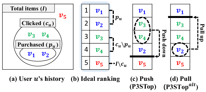
Figure 1: A toy example of the push/pull mechanism.

Toy Example. Figure 1a shows user $u$’s interaction history with items ($v_{1},v_{2},\\ v_{3},v_{4}$,$v_{5}$), and the ideal ranking list for user $u$ is displayed in Figure 1b. That is, for user $u$, we want to train our model so that the items are ordered in the following order at the end of the model training: P items ($\textbf{p}_{u}$), CBNP items ($\textbf{c}_{u}\char 92\relax\textbf{p}_{u}$), NC items ($\mathcal{I}\char 92\relax\textbf{c}_{u}$). Assuming that items are incorrectly ranked as in Figure 1c during the training process, we aim to push down as many incorrectly ranked CBNP (“negative”) items, i.e., $v_{3},v_{4}$, below the bound set by the last-ranked P (“positive”) item, i.e., $v_{2}$. In other words, we push down the relatively unreliable clicked items below the bound set by a solid purchased item, which makes our model more robust to unreliable click records. An alternative to the push mechanism (Figure 1c) is the pull mechanism (Figure 1d), which differs in the way that the bound is set. Precisely, it pulls up the purchased items, i.e., $v_{2}$, above the bound set by the first-ranked (“negative”) CBNP item, i.e., $v_{3}$, as shown in Figure 1d. This method is, however, prone to being dominated by unreliable click records, because the bound is set by the possibly unreliable clicked item. In Section 4.1 and 4.2, we will describe the rationale behind each case.

It is important to note that the above push mechanism in Figure 1c enables the model to particularly focus on the accuracy of the top-ranked items. More precisely, the upper bound of CBNP items ($v_{3},v_{4}$) is set to the last-ranked P item ($v_{2}$), which is the item that the user is more confident with than any CBNP item. In this regard, the bound set by a P item ($v_{2}$) (Figure 1c) should be relatively high and robust compared with the bound set by a clicked item ($v_{3}$) (Figure 1d). Therefore, pushing down the incorrectly ranked CBNP items below the last-ranked P item allows greater focus on the accuracy of the top-ranked items, because the bound set by the last-ranked P item is high and robust. We argue that our proposed method generates more practical recommendation results for users, since the top-ranked items get much more attention by users in practice [1]. However, only a few recent studies have particularly considered it for the task of recommendation [7, 14, 38].

Our main contributions are summarized as follows:

1. To complement the missing user–item interactions of purchase records, we formulate various model assumptions regarding the order of user preferences among non-purchased items by taking the click records into account (Section 3).

2. After we find a valid model assumption under the BPR model, we propose P3STop that is customized to be robust to relatively unreliable click records by particularly focusing on the accuracy of the top-ranked items. (Section 4).

3. Experimental results on two real-world e-commerce datasets demonstrate that P3STop considerably outperforms the state-of-the-art implicit feedback–based recommendation methods, especially for the top-ranked items. (Section 5).

It is worth noting that click records have been used for various tasks such as click-through rate (CTR) prediction in online advertising [29, 60, 57] and Twitter [21], user intent prediction [6, 28], repeat-buyer prediction [25], conversion response prediction in display advertising [24], and session–based click prediction [13]. However, not much effort has been devoted to purchase prediction, and to the best of our knowledge, our work is the first to propose a framework that leverages click records to complement the missing user–item interactions of purchase records.

Table 1: Notation

Symbol	Description
$\mathcal{U},\mathcal{I}$	Set of Users, Set of Items
$n,m$	Number of users and items
$\textbf{P}\in\mathbb{R}^{n\times m}$	User-Item Purchase matrix
$\textbf{C}\in\mathbb{R}^{n\times m}$	User-Item Click matrix
$\textbf{p}_{u}$	Items purchased by user $u$
$\textbf{c}_{u}$	Items clicked by user $u$
$K$	Number of latent dimensions
$\bm{\alpha\in\mathbb{R}}^{n\times K}$	User latent matrix
$\bm{\beta\in\mathbb{R}}^{m\times K}$	Item latent matrix
$\bm{\gamma\in\mathbb{R}}^{m}$	Item bias
${\lambda}$	The strength of the model regularization
${\eta}$	Learning rate

2 Problem Statement

We first introduce notations used throughout this paper (Table 1). Let $\mathcal{U}$ and $\mathcal{I}$ be the set of users and items, respectively, and we have $n$ users and $m$ items. The purchase records of users in $\mathcal{U}$ on items in $\mathcal{I}$ are represented by the purchase matrix $\textbf{P}={[{p_{ui}}]_{n\times m}}$, where ${p_{ui}=1}$ if user $u$ purchased item $i$, and 0 otherwise. Likewise, the click records of users in $\mathcal{U}$ on items in $\mathcal{I}$ are represented by the click matrix $\textbf{C}={[{c_{ui}}]_{n\times m}}$, where ${c_{ui}=1}$ if user $u$ clicked item $i$, and 0 otherwise; counts are ignored in this work. $\textbf{p}_{u}$ and $\textbf{c}_{u}$ denote the sets of items purchased and clicked by user $u$, respectively. We formally define our problem in this paper as follows:

Problem Definition
Given: The purchase matrix P and click matrix C,

Goal: To recommend items $i\in\mathcal{I}\textbackslash(\textbf{p}_{u}\cup\textbf{c}_{u})$ to each user $u\in\mathcal{U}$; among items that the user has not previously interacted with (neither purchased nor clicked).

3 Ordering User Preferences among Non-purchased Items

In this section, we describe our framework that leverages click records to complement the missing user–item interactions of purchase records. i.e., non-purchased items. We begin by explaining our model assumptions regarding the order of user preferences among non-purchased items (Section 3.1). Next, we describe how our model assumptions are implemented under the BPR model (Section 3.2). Then, we discuss two shortcomings of naively incorporating click records under the BPR model (Section 3.3).

3.1 Defining the Model Assumptions

Recall the AMAN assumption made by previous pairwise learning-to-rank methods [10, 34, 41].

AMAN Assumption.

We assume that a user prefers purchased items to non-purchased items.

$$i\succ_{u}j,\text{if}~{}i\in\textbf{p}_{u}\wedge j\in\mathcal{I}\char 92\relax\textbf{p}_{u}$$ (1)

Eqn. 1 implies that user $u$ prefers purchased items $i$ to non-purchased items $j$. However, this assumption is oversimplified in that all non-purchased items are equally considered as negative feedback, whereas in reality some of the non-purchased items attract the user more than the others.

To overcome the above limitation of the AMAN assumption, we incorporate users’ click records that reveal users’ general interest, assuming that users click on numerous items before making purchases. Although the user preference reflected therein is not as strong as in purchase records, we expect that click records will complement the missing user–item interactions of purchase records. To this end, given purchased items, we split the non-purchased items into two disjoint sets, i.e., clicked-but-not-purchased items and non-clicked items, by using click records, and introduce three different model assumptions regarding the order of user preferences among them. For each user $u$, we assume $\textbf{p}_{u}\subset\textbf{c}_{u}\subset\mathcal{I}$, i.e., all purchased items are selected from clicked items.

Assumption 1.

We assume that a user prefers purchased items to non-clicked items.

$$i\succ_{u}j,\text{if}~{}i\in\textbf{p}_{u}\wedge j\in\mathcal{I}\char 92\relax\textbf{c}_{u}$$ (2)

Instead of regarding non-purchased items as negative feedback as in Eqn. 1, this time we regard non-clicked items as negative feedback. This narrows down the candidates for negative feedback, i.e., from $\mathcal{I}\char 92\relax\textbf{p}_{u}$ to $\mathcal{I}\char 92\relax\textbf{c}_{u}$, which is expected to relieve the AMAN assumption.

Assumption 2.

We assume that a user prefers purchased items to clicked-but-not-purchased items, clicked-but-not purchased items to non-clicked items, and purchased items to non-clicked items.

$$i\succ_{u}j,\;j\succ_{u}k,\;i\succ_{u}k,\text{if}~{}i\in\textbf{p}_{u}\wedge j\in\textbf{c}_{u}\char 92\relax\textbf{p}_{u}\wedge k\in\mathcal{I}\char 92\relax\textbf{c}_{u}$$ (3)

We extend Assumption 1 by adding another set of items. i.e., clicked-but-not-purchased items ($\textbf{c}_{u}\char 92\relax\textbf{p}_{u}$). Eqn. 3 is based on the assumption that 1) user $u$ is more confident with purchased items ($\textbf{p}_{u}$) than to clicked-but-not-purchased items ($\textbf{c}_{u}\char 92\relax\textbf{p}_{u}$), because users generally decide to purchase items over many other candidates ($\textbf{c}_{u}\char 92\relax\textbf{p}_{u}$) that reveal users’ general interest, which implies that 2) user $u$ prefers clicked-but-not-purchased items to the items that are neither purchased nor clicked ($\mathcal{I}\char 92\relax\textbf{c}_{u}$).

Assumption 3.

We assume that a user prefers purchased items to clicked-but-not-purchased items, and non-clicked items to clicked-but-not-purchased items.

$$i\succ_{u}j,\;k\succ_{u}j,\;i\succ_{u}k,\text{if}~{}i\in\textbf{p}_{u}\wedge j\in\textbf{c}_{u}\char 92\relax\textbf{p}_{u}\wedge k\in\mathcal{I}\char 92\relax\textbf{c}_{u}$$ (4)

Eqn. 4 implies that user $u$ dislikes items that are clicked-but-not-purchased ($\textbf{c}_{u}\char 92\relax\textbf{p}_{u}$) more than those that are not clicked at all ($\mathcal{I}\char 92\relax\textbf{c}_{u}$). This assumption is also intuitive in the sense that although being aware of clicked-only items ($\textbf{c}_{u}\char 92\relax\textbf{p}_{u}$), the fact that the user still chose not to purchase them implies that the user dislikes them.

3.2 Verifying the Model Assumptions

To figure out which of our three model assumptions (Eqn. 2,3,4) is valid, we implement them under the BPR model [41], and name each of them P3S_1, P3S_2 and P3S_3, respectively (P3S stands for modeling pairwise relationships among three disjoint item sets). We only present here the equation for P3S_2, which is based on Assumption 2. The equations for P3S_1 and P3S_3 are similarly formulated and hence omitted. For each user $u$, we maximize the following loss function:

$$\begin{split}&{\mathcal{L}_{\textsf{P3S\_2}}}(u)=\sum\limits_{i\in{\textbf{p}_{u}}}{\sum\limits_{j\in{\textbf{c}_{u}}\backslash{\textbf{p}_{u}}}{\ln\sigma({{\hat{x}}_{uij}})}}\\ &+\sum\limits_{j\in{\textbf{c}_{u}}\backslash{\textbf{p}_{u}}}{\sum\limits_{k\in I\backslash{\textbf{c}_{u}}}{\ln\sigma({{\hat{x}}_{ujk}})}}+\sum\limits_{i\in{\textbf{p}_{u}}}{\sum\limits_{k\in I\backslash{\textbf{c}_{u}}}{\ln\sigma({{\hat{x}}_{uik}})}}\end{split}$$ (5)

where ${\hat{x}}_{uik}={\hat{x}}_{ui}-{\hat{x}}_{uk}$, and $\hat{x}_{ui}=\alpha_{u}^{T}\beta_{i}+\gamma_{i}$ denotes the predicted preference of user $u$ on item $i$ computed by matrix factorization (MF); $\alpha_{u}\in\mathbb{R}^{K}$ and $\beta_{i}\in\mathbb{R}^{K}$ represent the $K$-dimensional latent factors for user $u$ and item $i$, respectively, and $\gamma_{i}\in\mathbb{R}$ denotes the item bias term for item $i$. $\sigma({{\hat{x}}_{uij}})$ denotes the probability that user $u$ prefers item $i$ to item $j$ [41], which is approximated by a sigmoid function $\sigma(\cdot)$. For more details of the optimization process, refer to the original paper [41] that proposed the BPR model. We later show in our experiments (Table 4) that P3S_2 outperforms P3S_1 and P3S_3, which implies that Assumption 2 is the most valid model assumption.

Note that other scoring functions such as neural network (NN)–based functions  [12, 13, 20] can also be applied to our framework by simply replacing MF. However, as our focus is to propose a “framework” that can properly utilize click records for purchase prediction rather than to prove the superiority of NN over MF, we conduct experiments with MF as our scoring function in this paper.

3.3 Discussion: Shortcomings of P3S_2

Although P3S_2 is shown to be beneficial for purchase prediction when implemented under the BPR model, it has two shortcomings. The first shortcoming is caused by the relative unreliableness of click records, whose amount even greatly exceeds that of purchase records. Unlike purchases, clicks can occur even without a user’s intent to purchase; a user may accidentally click on wrong items or click on items out of simple curiosity, whereas a user is more confident with purchased items. That is to say, the click records are more likely to be irrelevant to user preferences than the purchase records. Therefore, we argue that relying too much on the relatively unreliable click records would be detrimental to the performance of recommendation. However, since BPR was developed for bipartite ranking in which every possible positive–negative instance pair is taken into account, the model can be easily dominated by the relatively unreliable click records as their amount greatly exceeds that of purchase records. The second shortcoming is caused by the objective of the BPR model. Although users are mainly interested in top-ranked items [1], BPR maximizes the AUC, which gives an equal weight to each training instance regardless of its position in the list. In other words, a mistake in the higher part of the recommendation list is equally penalized with one in the lower part, implying that optimizing the AUC does not allow a particular focus on the accuracy of the top-ranked items. Therefore, we propose a novel method that simultaneously addresses the above shortcomings.

4 The Proposed Method: P3STop

Here, we describe our novel learning-to-rank method, P3STop, that is customized to be robust to relatively unreliable click records by particularly focusing on the accuracy of the top-ranked items. Since P3S_2, which is based on Assumption 2, turned out to be the most valid model (Table 4), we adopt it as the underlying assumption of our proposed method, P3STop, hereinafter. Note that under Assumption 2, purchased (P) items and non-clicked (NC) items are always regarded as positive and negative items, respectively. In contrast, clicked-but-not-purchased (CBNP) items can be considered as either positive or negative items, depending on which pair of itemsets we are interested in. That is, CBNP items are considered as negative items when compared with P items, and are considered as positive items when compared with NC items.

4.1 Model Formulation

For each user $u$, we compute the sum of the number of 1) CBNP items ranked above the least relevant P item, 2) NC items ranked above the least relevant CBNP item, and 3) NC items ranked above the least relevant P item, and minimize the sum as following:

$$\small\begin{split}\mathcal{L}_{\textsf{P3STop}}(u)&=\frac{1}{{|{\textbf{c}_{u}}\char 92\relax{\textbf{p}_{u}}|}}\sum\limits_{j\in{\textbf{c}_{u}}\char 92\relax{\textbf{p}_{u}}}\mathbb{I}{\left[(\mathop{\min}\limits_{i\in{\textbf{p}_{u}}}{\hat{x}_{ui}})\leq{\hat{x}_{uj}}\right]}\\ &+\frac{1}{{|I\char 92\relax{\textbf{c}_{u}}|}}\sum\limits_{k\in I\char 92\relax{\textbf{c}_{u}}}\mathbb{I}{\left[(\mathop{\min}\limits_{j\in{\textbf{c}_{u}}\char 92\relax{\textbf{p}_{u}}}{\hat{x}_{uj}})\leq{\hat{x}_{uk}}\right]}\\ &+\frac{1}{{|I\char 92\relax{\textbf{c}_{u}}|}}\sum\limits_{k\in I\char 92\relax{\textbf{c}_{u}}}\mathbb{I}\left[(\mathop{\min}\limits_{i\in{\textbf{p}_{u}}}{\hat{x}_{ui}})\leq{\hat{x}_{uk}}\right]\\ &=\frac{1}{{|{\textbf{c}_{u}}\char 92\relax{\textbf{p}_{u}}|}}\sum\limits_{j\in{\textbf{c}_{u}}\char 92\relax{\textbf{p}_{u}}}{max\left[0,1-((\mathop{\min}\limits_{i\in{\textbf{p}_{u}}}{\hat{x}_{ui}})-{\hat{x}_{uj}})\right]}\\ &+\frac{1}{{|I\char 92\relax{\textbf{c}_{u}}|}}\sum\limits_{k\in I\char 92\relax{\textbf{c}_{u}}}max{\left[0,1-((\mathop{\min}\limits_{j\in{\textbf{c}_{u}}\char 92\relax{\textbf{p}_{u}}}{\hat{x}_{uj}})-{\hat{x}_{uk}})\right]}\\ &+\frac{1}{{|I\char 92\relax{\textbf{c}_{u}}|}}\sum\limits_{k\in I\char 92\relax{\textbf{c}_{u}}}max\left[0,1-((\mathop{\min}\limits_{i\in{\textbf{p}_{u}}}{\hat{x}_{ui}})-{\hat{x}_{uk}})\right]\end{split}$$ (6)

where $\hat{x}_{ui}=\alpha_{u}^{T}\beta_{i}$ and $\mathbb{I}[\cdot]$ is the indicator function that returns 1 if the argument is true, otherwise 0. Note that in Eqn. 6 the bound is set with respect to positive items and thus more emphasis is placed on positive items than on negative items, making our model robust to relatively unreliable negative items. For example, consider the first term, where for user $u$, we set the upper bound of the CBNP items $j$ ($\in\textbf{c}_{u}\char 92\relax\textbf{p}_{u}$) to the score of the last-ranked P item $({\min_{i\in{{\mathbf{p}}_{u}}}}{{\hat{x}}_{ui}})$ (Figure 1c). Although the last-ranked P item $i$ has the lowest score among all P items $\mathbf{p}_{u}$, its score (${\min_{i\in{{\mathbf{p}}_{u}}}}{{\hat{x}}_{ui}}$) should be higher than the score ($\hat{x}_{uj}$) of any CBNP item $j$ ($\in{\textbf{c}_{u}}\char 92\relax{\textbf{p}_{u}}$) because it was specifically chosen by user $u$ from all the clicked items (Assumption 2). Consequently, the upper bound set by the last-ranked positive item will be high enough so that we obtain positive items near the top by pushing down relatively unreliable negative items below it. In summary, by minimizing $\mathcal{L}_{\textsf{P3STop}}(u)$ for each user, we aim to put as many unreliable negative items below positive items as possible, which results in high accuracy especially for the top-ranked items. As for the optimization of Eqn. 6, since $\mathbb{I}[\cdot]$ is non-convex, making the optimization process difficult because of its discrete nature, we replace it with the hinge loss function $\ell(x)=max(0,1-x)$, which is a widely used convex surrogate for the indicator function [44].

Optimization Objective. Given the loss function $\mathcal{L}_{\textsf{P3STop}}(u)$ for each user $u\in\mathcal{U}$ as in Eqn. 6, the final objective function to minimize is formulated as follows:

$$\mathcal{J}_{\textsf{P3STop}}(\Theta)=\frac{1}{{|\mathcal{U}|}}\sum_{u\in\mathcal{U}}\mathcal{L}_{\textsf{P3STop}}(u)+\frac{\lambda_{\alpha}}{2}\sum_{u\in\mathcal{U}}||\alpha_{u}||_{2}^{2}+\frac{\lambda_{\beta}}{2}\sum_{i\in\mathcal{I}}||{\beta_{i}}||_{2}^{2}$$ (7)

where $\lambda_{\alpha}$ and $\lambda_{\beta}$ are regularization parameters for the user and for the item latent factors, respectively. We set $\lambda_{\alpha}=\lambda_{\beta}=\lambda$ to reduce the model complexity. We adopt the widely used stochastic gradient descent (SGD) method to optimize the objective function in Eqn. 7. For each user $u$, we first sample a triple $(i,j,k)$ from the training set $\mathcal{O}=\{\mathcal{O}_{u}|u\in|\mathcal{U}|\}$ where $\mathcal{O}_{u}=\{(i,j,k)|i\in\textbf{p}_{u}\wedge j\in\textbf{c}_{u}\char 92\relax\textbf{p}_{u}\wedge k\in\mathcal{I}\char 92\relax\textbf{c}_{u}\}$ , $\mathcal{O}_{u}$ denoting the training set for user $u$. We compute the gradient for each parameter in $\Theta$, i.e., $\alpha_{u},\beta_{i},\beta_{j},\beta_{k}$, and update each of them by using SGD. The gradient for each parameter is computed as follows:

• The gradient of $\alpha_{u}$ for $u\in\mathcal{U}$:

  $$\begin{split}&\frac{{\partial L_{\textsf{P3STop}}(u)}}{{\partial{\alpha_{u}}}}=\mathbb{I}[{(\mathop{\min}\limits_{i\in{\textbf{p}_{u}}}{\hat{x}_{ui}})-{\hat{x}_{uj}}\leq 1]}\left({\beta_{j}}-\frac{{\partial\mathop{\min}\limits_{i\in{\textbf{p}_{u}}}{\hat{x}_{ui}}}}{{\partial{\alpha_{u}}}}\right)\\ &+\mathbb{I}{[(\mathop{\min}\limits_{j\in{\textbf{c}_{u}}\char 92\relax{\textbf{p}_{u}}}{\hat{x}_{uj}})-{\hat{x}_{uk}}\leq 1]}\left({\beta_{k}}-\frac{{\partial\mathop{\min}\limits_{j\in{\textbf{c}_{u}}\char 92\relax{\textbf{p}_{u}}}{\hat{x}_{uj}}}}{{\partial{\alpha_{u}}}}\right)\\ &+\mathbb{I}{[(\mathop{\min}\limits_{i\in{\textbf{p}_{u}}}{\hat{x}_{ui}})-{\hat{x}_{uk}}\leq 1]}\left({\beta_{k}}-\frac{{\partial\mathop{\min}\limits_{i\in{\textbf{p}_{u}}}{\hat{x}_{ui}}}}{{\partial{\alpha_{u}}}}\right)\end{split}$$ (8)

• The gradient of $\beta_{i}$ for $i\in\textbf{p}_{u}$

  $$\begin{split}\frac{{\partial\mathcal{L}_{\textsf{P3STop}}(u)}}{{\partial{\beta_{i}}}}&=\mathbb{I}{\left[{(\mathop{\min}\limits_{i\in{\textbf{p}_{u}}}{\hat{x}_{ui}})-{\hat{x}_{uj}}\leq 1}\right]}\left({-\frac{{\partial\mathop{\min}\limits_{i\in{\textbf{p}_{u}}}{\hat{x}_{ui}}}}{{\partial{\beta_{i}}}}}\right)\\ &+\mathbb{I}{\left[{(\mathop{\min}\limits_{i\in{\textbf{p}_{u}}}{\hat{x}_{ui}})-{\hat{x}_{uk}}\leq 1}\right]}\left({-\frac{{\partial\mathop{\min}\limits_{i\in{\textbf{p}_{u}}}{\hat{x}_{ui}}}}{{\partial{\beta_{i}}}}}\right)\end{split}$$ (9)

• The gradient of $\beta_{j}$ for $j\in\textbf{c}_{u}\char 92\relax\textbf{p}_{u}$

  $$\begin{split}\frac{{\partial\mathcal{L}_{\textsf{P3STop}}(u)}}{{\partial{\beta_{j}}}}&=\mathbb{I}[{(\mathop{\min}\limits_{i\in{\textbf{p}_{u}}}{\hat{x}_{ui}})-{\hat{x}_{uj}}\leq 1}]({{\alpha_{u}}})\\ &+\mathbb{I}{\left[{(\mathop{\min}\limits_{j\in{\textbf{c}_{u}}\char 92\relax{\textbf{p}_{u}}}{\hat{x}_{uj}})-{\hat{x}_{uk}}\leq 1}\right]}\left({-\frac{{\partial\mathop{\min}\limits_{j\in{\textbf{c}_{u}}\char 92\relax{\textbf{p}_{u}}}{\hat{x}_{uj}}}}{{\partial{\beta_{j}}}}}\right)\end{split}$$ (10)

• The gradient of $\beta_{k}$ for $k\in\mathcal{I}\char 92\relax\textbf{c}_{u}$

  $$\begin{split}\frac{{\partial\mathcal{L}_{\textsf{P3STop}}(u)}}{{\partial{\beta_{k}}}}&=\mathbb{I}{[(\mathop{\min}\limits_{j\in{\textbf{c}_{u}}\char 92\relax{\textbf{p}_{u}}}{\hat{x}_{uj}})-{\hat{x}_{uk}}\leq 1]}({\alpha_{u}})\\ &+\mathbb{I}{[(\mathop{\min}\limits_{i\in{\textbf{p}_{u}}}{\hat{x}_{ui}})-{\hat{x}_{uk}}\leq 1]}({\alpha_{u}})\end{split}$$ (11)

Note that the derivatives given by:

$$\begin{dcases}\frac{{\partial\mathop{\min}\limits_{i\in{X}}{\hat{x}_{ui}}}}{{\partial{\alpha_{u}}}}=\beta_{i}\text{, where }\alpha_{u}^{T}\beta_{i}\text{ is the minimum for }i\in X\\ \frac{{\partial\mathop{\min}\limits_{i\in X}{\hat{x}_{ui}}}}{{\partial{\beta_{i}}}}=\alpha_{u}\end{dcases}$$ (12)

where $X\in\{\textbf{p}_{u},{\textbf{c}_{u}}\char 92\relax{\textbf{p}_{u}}\}$.

4.2 Alternative Method: P3STop^alt

As an alternative to our proposed method P3STop, we can consider another method that relies more heavily on click records. For each user $u$, we compute the sum of the number of 1) P items ranked below the most relevant CBNP item, 2) CBNP items ranked below the most relevant NC item, and 3) P items ranked below the most relevant NC item, and minimize the sum as follows:

$$\begin{split}\mathcal{L}_{\textsf{P3STop${}^{alt}$}}(u)&=\frac{1}{{|{\textbf{p}_{u}}|}}\sum\limits_{i\in{\textbf{p}_{u}}}\mathbb{I}{\left[{{\hat{x}_{ui}}\leq(\mathop{\max}\limits_{j\in{\textbf{c}_{u}}\char 92\relax{\textbf{p}_{u}}}{\hat{x}_{uj}}})\right]}\\ &+\frac{1}{{|{\textbf{c}_{u}}\char 92\relax{\textbf{p}_{u}}|}}\sum\limits_{j\in{\textbf{c}_{u}}\char 92\relax{\textbf{p}_{u}}}\mathbb{I}{\left[{{\hat{x}_{uj}}\leq(\mathop{\max}\limits_{k\in I\char 92\relax{\textbf{c}_{u}}}{\hat{x}_{uk}}})\right]}\\ &+\frac{1}{{|{\textbf{p}_{u}}|}}\sum\limits_{i\in{\textbf{p}_{u}}}\mathbb{I}{\left[{{\hat{x}_{ui}}\leq(\mathop{\max}\limits_{k\in I\char 92\relax{\textbf{c}_{u}}}{\hat{x}_{uk}}})\right]}\end{split}$$ (13)

This method, named P3STop^alt, is distinguished from P3STop in that P3STop^alt resorts to the negative items to set the bound. To be precise, it sets the lower bound of the positive items to the score of the top-ranked negative item; as opposed to P3STop that sets the upper bound of negative items to the last-ranked positive item. Here, we want the lower bound to be high enough so that pulling up the positive items above it is meaningful (Figure 1d). However, the negative items always include relatively unreliable click records in this case, and thus the lower bound set by the negative items is not guaranteed to be sufficiently high and robust; in contrast to high and robust bound of P3STop set by positive items. This implies that pulling up positive items above relatively low bound would not yield high accuracy at the top. We later present the performance of P3STop^alt in the experiments (Table 5) to show the unreliableness of click records compared with purchase records. We note that P3STop^alt is an enhanced version of Inf-Push [7], whose underlying AMAN assumption is replaced with Assumption 2 [23].

Complexity Analysis. Another benefit of P3STop is the improved time complexity compared with previous pairwise methods developed for bipartite ranking, such as BPR and P3S. More precisely, the time complexity of evaluating P3S_2 is $O(|\textbf{p}_{u}||\textbf{c}_{u}\char 92\relax\textbf{p}_{u}|+|\textbf{c}_{u}\char 92\relax\textbf{p}_{u}||\mathcal{I}\char 92\relax\textbf{c}_{u}|+|\textbf{p}_{u}||\mathcal{I}\char 92\relax\textbf{c}_{u}|)=O(m^{2})$ whereas that for P3STop is $O(2\times(|\textbf{p}_{u}|+|\textbf{c}_{u}\char 92\relax\textbf{p}_{u}|+|\mathcal{I}\char 92\relax\textbf{c}_{u}|))=O(m)$, which will become clear when converted into a dual form [23]. We refer the readers to Section 3 of [23] for the detailed proof regarding the entire process of converting a bipartite ranking into a dual formulation, which in turn gives us the time complexity linear in the number of items.

5 Experiments

The experiments are designed to answer the following research questions (RQs):

1. Are click records useful for purchase prediction?

2. Does P3STop indeed focus on the accuracy near the top?

3. Is P3STop robust to unreliable click records?

4. How does the latent dimensionality affect the performance?

5. Does P3STop outperform baselines without compromising the novelty of item recommendations?

5.1 Experimental Settings

Dataset. We evaluated our proposed method on two real-world datasets each of which contains both purchase records and click records for the same set of users. The RecSys2015 dataset consists of sessions of click and purchase sequences extracted from an e-commerce website, where we regard each session is as a user. To the best of our knowledge, the RecSys2015 dataset is the only public dataset in which a user is provided with both the purchase and click records, and hence we ran experiments on a proprietary dataset from NAVER shopping, which is a web portal that provides a platform for online shopping. We collected users’ click and purchase records for three months (Jan. 2017 through Mar. 2017). For both datasets, we removed users having fewer than five purchases and twenty clicks. Moreover, to filter out possible abusing users and items in both datasets, we removed the top 0.001% of users and items in terms of the number of observations. After preprocessing, the RecSys2015 dataset contained 30,867 purchase records on 5,869 items and 102,939 click records on 11,071 items from 7,076 users, and the NAVER shopping dataset contained 23,373 purchase records on 6,743 items and 243,908 click records on 10,738 items from 5,317 users.

Methods Compared.

• BPR [41]: A pairwise learning-to-rank method based on the AMAN assumption as in Eqn. 1.

• SLIM [32]: An extension of itemKNN [45] that models the user’s preference for item $i$ as a weighted combination of the user’s preference for item $j$ and the item similarity between $i$ and $j$. It learns a item-item similarity matrix from the data.

• CLiMF [46]: A collaborative ranking method for implicit feedback that directly maximizes Mean Reciprocal Rank (MRR).

• PMF [30]: An MF–based pointwise method that minimizes the rating prediction error. As PMF is a common baseline method for rating prediction, we modify it to model click and purchase records; we assign 1 to clicked items, and 2 to purchased items.

• eALS [11]: The state-of-the-art sampling–based MF method that samples non-purchased items based on their popularity, which is shown to surpass the uniform weighting scheme [15].

• GRU4REC [13]: State-of-the-art session–based click prediction method based on GRU. As its goal (click prediction) differs from ours (purchase prediction), we added a fully connected layer at the end of last hidden state of GRU4REC for predicting the purchased items.

• P3S_1, P3S_2, P3S_3, P3STop, P3STop^alt: Our proposed methods based on Eqn. 2, 3, 4, 6, and 13, respectively. Note that P3S_2 degenerates to BPR when click records are not provided.

• Inf-Push [7]: A collaborative ranking method based on explicit feedback that focuses on the ranking performance at the top. Because this method was originally designed for explicit feedback, we cannot directly compare it with our proposed method. Instead, we treat purchased items as relevant and all the non-purchased items as non-relevant.

• P3STop^mix: A method that jointly minimizes the objective functions of P3STop
  and P3STop^alt as $(1-\varepsilon)\cdot\mathcal{L}_{\textsf{P3STop}}(u)+\varepsilon\cdot\mathcal{L}_{\textsf{P3STop${}^{alt}$}}(u)$, where $\varepsilon=0.5$.

Since our goal is not the click prediction but the purchase prediction, our baseline competitors are built using the purchase records; except for PMF. In fact, we tried the “click–based purchase prediction” for BPR (using only click records instead of purchase records to predict purchases) to see how helpful click records are for purchase prediction. However, its performance turned out to be very poor, and hence excluded in the paper. Moreover, we assume that explicit feedback such as ratings are not provided, and thus we compare our methods with implicit feedback–based methods.

Evaluation Setting. We adopt the leave-one-out evaluation, which has been widely used in literature [10, 12, 11, 41]. More precisely, for both datasets, we 1) chronologically ordered the sequence of purchase data and used the last records as test data and the remainder as training data, and 2) used the click records of the user up to the timestamp of the last purchase in the training data and discarded the rest. It is worth mentioning that as our target is purchase prediction, where the goal is to predict an item to be purchased in the future, randomly splitting the dataset is unrealistic. Precisely, if we randomly sample a purchased item for each user (without considering the purchased order) and use the rest of the purchased items for training, we will be predicting a past event by using future events. Therefore, for each user, we held out the latest purchased item as the test data, and thus we cannot apply conventional cross-validation. Instead, we ran the experiments five times with different random seeds for initialization for reliability of the results.

Predicting users’ future purchase among clicked items is rather a trivial task, and obviously the performance is expected to be significantly improved by incorporating users’ click record as in our method, because items are purchased from clicked items. Indeed, our method greatly outperformed the competitors under such setting. Therefore, to make the problem more challenging and practical [42], we evaluate our method on how well it predicts users’ future purchase among non-clicked items. That is to say, the candidate items for recommendation for each user are the items that are neither clicked nor purchased by the user in the past.

Evaluation Metrics. As our objective is to optimize the accuracy at the top, we measured the ranking performance using three metrics that emphasize the accuracy at the top (Recall@$N$, NDCG@$N$, MRR@$N$ [8, 39, 56]) when $N$ is small, and one that does not (AUC). Moreover, since there is only one relelevant item for each user, and that we are dealing with implicit feedback datasets, MRR and NDCG provide the same insight. However, we included both of them because they are the two most popularly used metrics in recommender system research. Precision is not employed because each user has only one test data in which case Precision is proportional to Recall. We do not consider metrics, such as RMSE and MAE, as they are suitable for explicit feedback datasets [9, 18], but not for implicit feedback datasets. Recall that we split our data into training/validation/test sets by selecting for each user $u$ a random item to be used for validation $\mathcal{V}_{u}$ and another for testing $\mathcal{T}_{u}$. All remaining data is used for training. The predicted ranking is evaluated on $\mathcal{T}_{u}$ with various ranking metrics. Metrics used for evaluation are described as follows:

• Recall@N: The average of the ratio of all relevant items included in top-N of the recommended list of items for each user.
  

  $$Recall@N=\frac{1}{n}\sum\limits_{u\in U}{\frac{{|rel(u,N)|}}{|rel(u)|}}$$

  where $rel(u,N)$ denotes the relevant (purchased) items among top-N recommended items, and $rel(u)$ denotes relevant (purchased) items of user $u$ in the test set.

• Normalized Discounted Cumulative Gain (NDCG)
  

  $$NDCG=\frac{1}{n}\sum\limits_{u\in U}{\frac{{DC{G_{u}}}}{{IDC{G_{u}}}}}$$

  where DCG and IDCG (Ideal DCG) are represented as:

  $$DC{G_{u}}=\sum\limits_{i\in rel(u)}{\frac{1}{{{{\log}_{2}}(rank_{i}^{u}+1)}}}$$

  $$IDCG_{u}=\sum\limits_{i\in rel(u)}{\frac{1}{{{{\log}_{2}}(i+1)}}}$$

  where $rank_{i}^{u}$ denotes the rank of item $i$ in user $u$’s recommendation list.

• Mean Reciprocal Rank (MRR)
  

  $$MRR=\frac{1}{n}\sum\limits_{u\in U}{\frac{1}{{ran{k^{u}}}}}$$

  where $rank_{u}$ denotes the first rank of the relevant item in the recommended list of user $u$.

• Area Under ROC Curve (AUC)
  

  $$AUC=\frac{1}{n}\sum\limits_{u\in U}{\frac{1}{{|E(u)|}}\sum\limits_{(i,j)\in{E_{u}}}{\mathbb{I}[{\hat{x}_{ui}}>{\hat{x}_{uj}}]}}$$

  where $E(u)=\left\{(i,j)|(u,i)\in\mathcal{T}_{u}\wedge(u,j)\notin\left(\mathcal{P}_{u}\cup\mathcal{V}_{u}\cup\mathcal{T}_{u}\right)\right\}$ and $\mathbb{I}[\cdot]$ is an indicator function that is equal to 1 if the argument is true. $({\hat{x}_{ui}}>{\hat{x}_{uj}})$ indicates that the rank of item $i$ is higher than that of item $j$ for user $u$.

Note that if we were not to focus on the top ranks, and if we had more than one relevant item for each user, it would be more rational to test on deeper cut-offs due to the robustness [50]. But in this work, we mainly focus on the accuracy on the top ranks, and thus test on relatively shallow cut-offs. i.e., $N=10,20$.

In addition to the conventional ranking metrics described above, we also evaluate on the novelty of the item recommendations provided by our method. To this end, we adopt self-information (SI) [2, 59], which measures the unexpectedness of an item recommendation relative to its global popularity:

$$\text{SI}=\frac{1}{|\mathcal{U}|}\sum\limits_{u\in U}\frac{1}{|L(u)|}\sum\limits_{i\in L(u)}-\log_{2}\frac{C(i)}{|\mathcal{U}|}$$ (14)

where $L(u)$ denotes a list of item recommendations for user $u$, $C(i)$ denotes the number of users that purchased item $i$.

Table 2: Best performing hyperparameter values. Note that SLIM has two hyparparameters for regularizations (L1/L2).

Data	RecSys2015			Naver Shopping
Method	$K$	$\eta$	$\lambda$	$K$	$\eta$	$\lambda$
eALS	160	0.01	0.1	150	0.01	0.01
BPR	190	0.1	0.01	70	0.01	0.1
SLIM	150	-	0.01/5	150	-	0.01/3
CLiMF	60	0.05	0.5	190	0.1	0.1
PMF	160	0.01	0.1	170	0.01	0.1
GRU4REC	150	0.01	-	150	0.01	-
Inf-Push	190	0.01	0.01	180	0.1	0.01
P3S_2	180	0.05	0.01	200	0.01	0.01
P3STop	180	0.01	0.01	160	0.1	0.01

Table 3: Performance comparisons for different methods. (Imp.: improvement over the best competitor.)

RecSys2015
Metric	eALS	BPR	SLIM	CLiMF	PMF	GRU4REC	P3S_2	P3STop	Imp.
Recall@10	0.2132$\pm 0.0006$	0.2801$\pm 0.0011$	0.2417$\pm 0.0010$	0.0015$\pm 0.0007$	0.2280$\pm 0.0024$	0.1916$\pm 0.0018$	0.2955$\pm 0.0021$	0.3119$\pm 0.0047$	11.35%
Recall@20	0.2549$\pm 0.0008$	0.3489$\pm 0.0012$	0.2919$\pm 0.0007$	0.0022$\pm 0.0008$	0.2883$\pm 0.0034$	0.2580$\pm 0.0015$	0.3853$\pm 0.0011$	0.3959$\pm 0.0068$	13.47%
NDCG@10	0.1405$\pm 0.0004$	0.1792$\pm 0.0010$	0.1622$\pm 0.0011$	0.0007$\pm 0.0003$	0.1418$\pm 0.0019$	0.0895$\pm 0.0010$	0.1778$\pm 0.0017$	0.1913$\pm 0.0050$	6.75%
NDCG@20	0.1499$\pm 0.0006$	0.1966$\pm 0.0009$	0.1750$\pm 0.0014$	0.0008$\pm 0.0003$	0.1566$\pm 0.0017$	0.1063$\pm 0.0007$	0.2006$\pm 0.0011$	0.2125$\pm 0.0055$	8.09%
MRR@10	0.1178$\pm 0.0005$	0.1483$\pm 0.0009$	0.1374$\pm 0.0013$	0.0005$\pm 0.0003$	0.1154$\pm 0.0020$	0.0585$\pm 0.0009$	0.1425$\pm 0.0012$	0.1542$\pm 0.0051$	3.98%
MRR@20	0.1204$\pm 0.0004$	0.1531$\pm 0.0009$	0.1409$\pm 0.0002$	0.0006$\pm 0.0003$	0.1194$\pm 0.0019$	0.0631$\pm 0.0008$	0.1483$\pm 0.0014$	0.1600$\pm 0.0052$	4.51%
AUC	0.7914$\pm 0.0006$	0.8714$\pm 0.0005$	0.7012$\pm 0.0213$	0.5523$\pm 0.0380$	0.8688$\pm 0.0130$	0.7957$\pm 0.0009$	0.9083$\pm 0.0009$	0.8771$\pm 0.0008$	4.23%
NAVER Shopping
Recall@10	0.0475$\pm 0.0003$	0.0608$\pm 0.0010$	0.02914$\pm 0.0031$	0.0076$\pm 0.0038$	0.0360$\pm 0.0017$	0.0466$\pm 0.0022$	0.0618$\pm 0.0022$	0.0690$\pm 0.0015$	13.49%
Recall@20	0.0739$\pm 0.0005$	0.1031$\pm 0.0011$	0.0473$\pm 0.0012$	0.0115$\pm 0.0039$	0.0646$\pm 0.0030$	0.0750$\pm 0.0036$	0.1074$\pm 0.0024$	0.1130$\pm 0.0029$	9.60%
NDCG@10	0.0222$\pm 0.0001$	0.0311$\pm 0.0004$	0.0142$\pm 0.0014$	0.0040$\pm 0.0029$	0.0180$\pm 0.0005$	0.0220$\pm 0.0015$	0.0331$\pm 0.0004$	0.0350$\pm 0.0007$	12.54%
NDCG@20	0.0288$\pm 0.0002$	0.0417$\pm 0.0007$	0.0187$\pm 0.0007$	0.0049$\pm 0.0025$	0.0244$\pm 0.0009$	0.0291$\pm 0.0017$	0.0443$\pm 0.0003$	0.0460$\pm 0.0008$	10.31%
MRR@10	0.0147$\pm 0.0001$	0.0224$\pm 0.0007$	0.0097$\pm 0.0008$	0.0029$\pm 0.0029$	0.0126$\pm 0.0005$	0.0147$\pm 0.0013$	0.0233$\pm 0.0003$	0.0244$\pm 0.0010$	8.93%
MRR@20	0.0165$\pm 0.0001$	0.0252$\pm 0.0008$	0.0109$\pm 0.0006$	0.0032$\pm 0.0028$	0.0143$\pm 0.0006$	0.0166$\pm 0.0013$	0.0263$\pm 0.0004$	0.0274$\pm 0.0010$	8.73%
AUC	0.7371$\pm 0.0156$	0.8622$\pm 0.0018$	0.6340$\pm 0.0212$	0.7942$\pm 0.0156$	0.8520$\pm 0.0003$	0.7233$\pm 0.0011$	0.9420$\pm 0.0005$	0.8515$\pm 0.0014$	9.26%

Implementation. To make fair comparisons, we built on one of the most widely used library for recommender systems, called LibRec. We used their implementations of BPR, SLIM, CLiMF and PMF, and implemented eALS, variants of P3S and P3STop. We used PyTorch [36] to implement GRU4REC.

Parameters. For all baselines, we tuned the hyperparameters by performing grid searches with $K\in\{10,20,...,200\}$, and $\eta$ (learning rate)$,\lambda\in\{0.01,0.05,0.1\}$. For each user, we used the last purchased item as test data and the remainder as training data. Therefore, conventional cross-validation is not applicable here, as the data must be split based on time. Instead, we made a validation dataset by using the last purchased item of training data, and performed grid search on the validation dataset for five times with different random seeds for initialization to find the best hyperparameters. The best performing hyperparameter values for each method found by grid search on the validation dataset are summarized in Table 2. For experiments, we report the mean and the standard deviation over five runs with different random seeds for initialization; the standard deviations in graphs are displayed as error bars.

Table 4: Comparisons of different assumptions for P3S.

Data	Metric	P3S_1	P3S_2	P3S_3
RecSys2015	Recall@10	0.2772$\pm 0.0009$	0.2955$\pm 0.0021$	0.0017$\pm 0.0004$
	NDCG@10	0.1773$\pm 0.0005$	0.1778$\pm 0.0017$	0.0014$\pm 0.0003$
	MRR@10	0.1463$\pm 0.0006$	0.1425$\pm 0.0012$	0.0011$\pm 0.0003$
	AUC	0.8716$\pm 0.0006$	0.9083$\pm 0.0009$	0.4602$\pm 0.0035$
Naver Shopping	Recall@10	0.0602$\pm 0.0016$	0.0618$\pm 0.0022$	0.0028$\pm 0.0010$
	NDCG@10	0.0298$\pm 0.0006$	0.0331$\pm 0.0004$	0.0013$\pm 0.0007$
	MRR@10	0.0215$\pm 0.0006$	0.0233$\pm 0.0003$	0.0009$\pm 0.0006$
	AUC	0.8765$\pm 0.0029$	0.9420$\pm 0.0005$	0.4948$\pm 0.0050$

5.2 Performance Analysis

RQ1) Usefulness of Click Records. We begin by showing which of our model assumptions (Eqn. 2,3, or 4) performed the best in Table 4. We observe that P3S_2, which is based on Assumption 2 (Eqn. 3), generally outperforms P3S_1 and P3S_3 on both datasets, with P3S_3 performing extremely poorly. This implies that clicked-but-not-purchased items of a user are definitely more helpful in eliciting the user’s preference than non-clicked items, and thus this relationship should be taken into account for purchase prediction.

Given that P3S_2 is the right choice among the P3Ss, we now compare its performance with state-of-the-art implicit feedback based–recommendation methods in Table 5.1. We observe that P3S_2  consistently outperformed the purchase record–based baselines, i.e., eALS, CLiMF and BPR, with very few exceptions. This indicates that when click records are properly combined with purchase records to define the order of user preferences among non-purchased items, we can complement the missing user–item interactions of purchase records, which eventually leads to better recommendation quality. Other observations from Table 5.1 are as follows: 1) BPR consistently outperformed PMF. Although PMF utilizes both the click and purchase records for making recommendations, it performed worse than BPR, which leverages only the purchase records. This indicates that we should meticulously design a method when jointly modeling both the click and purchase records, which in fact was one of the objectives for this study. 2) GRU4REC, which is a click-based purchase prediction method, generally performs worse than other methods based on either only purchase or both click and purchase. This shows that while click records can be directly used for click prediction as in [13], using only click records for purchase prediction limits the prediction performance because click records are relatively weaker signal than purchases, which corroborates the benefit of our model assumptions for purchase prediction. However, we note that GRU4REC performs better than click–based version of BPR (not shown in Table 5.1), confirming the advantage of considering the sequential information of click records by using GRU. 3) BPR consistently outperformed eALS. This demonstrates the superiority of the pairwise learning-to-rank method upon which our method is built. 4) Although we expected CLiMF to perform better than BPR as in the original study [46], its performance turned out to be very poor. We attribute this poor performance to the difference in the target task, which leads to a different model formulation. More precisely, CLiMF ignores all the missing user–item interactions and only considers positive feedback, and we argue that this can be effective for tasks with sufficient positive feedback such as friend recommendations (about 70 friends per user on average for the datasets used by [46]). However, the poor performance of CLiMF in our task implies that this formulation is not appropriate for purchase prediction where the amount of positive feedback is usually small (four purchased items per user on average for the datasets used in this work). In addition, the poor performance of CLiMF compared with BPR, which leverages the negative feedback, corroborates the importance of leveraging negative feedback in different target tasks. 5) SLIM performs relatively better on RecSys2015 dataset compared with NAVER dataset. Precisely, on Recsys2015 dataset, SLIM performs the second best among the baselines, whereas it performs worse on NAVER dataset. This is mainly because SLIM can only model relations between items that have been co-purchased by at least some users, which implies that SLIM performs well on dense datasets than on sparse datasets [16]. In the same vein, we attribute the inferior performance of SLIM compared with BPR to the sparseness of our datasets.

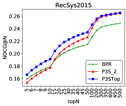
Figure 2: Comparisons over various $N$s (RecSys2015).

RQ2) Focus on the Accuracy of the Top-Ranked Items. We observe from Figure 2 that although P3S_2 outperforms BPR for relatively large $N$s ($N\geq 20$), their performance is similar to BPR for smaller $N$s less than 10; in this range, BPR even performs better than P3S_2. However, providing accurate recommendations in the lower part of the recommendation list as P3S_2 is not desired for e-commerce stores because users are mainly interested in the top-ranked items in practice [1]. Recall that the objective of our ultimate proposed method, P3STop, is to focus on the accuracy of the top-ranked items. The following observations are made regarding the performance of P3STop: 1) From Table 5.1, in terms of Recall, NDCG and MRR, P3STop considerably outperforms all competitors including P3S_2 for $N=10,20$, which are relatively small $N$s. 2) More importantly, for even smaller $N$s less than 10 (Figure 2), we observe that P3STop still outperforms both BPR and P3S_2, whereas for large $N$s ($N\geq 30$), the performance gap between P3S_2  and P3STop starts to get smaller, and the performance of P3STop almost equals to that of P3S_2 above $N=$ 300. This implies that P3STop focuses on the accuracy of the top-ranked items ($N\leq 20$) at the expense of the accuracy in the lower part of the recommendation list ($N\geq 30$), which answers RQ2. We observed similar results for other metrics as well. 3) Above results are corroborated by the performance in terms of AUC, a metric that treats a mistake in the higher part of the recommendation list as equal to one the lower part. More precisely, P3S_2 consistently outperforms P3STop in both datasets in terms of AUC, which implies that P3S_2 provides a more balanced recommendation list; this conversely shows that P3S_2 does not particularly focus on the top. We attribute this performance to the fact that P3S_2 is built upon the BPR model, whose objective is to optimize for the AUC metric (Eqn. 5).

Table 5: Comparisons among “push” algorithms.

RecSys2015
Metric	Inf-Push	P3STop	P3STopalt	P3STopmix
R@10	0.1631$\pm 0.0018$	0.3119$\pm 0.0047$	0.1891$\pm 0.0034$	0.1842$\pm 0.0024$
N@10	0.0818$\pm 0.0011$	0.1913$\pm 0.0050$	0.1021$\pm 0.0032$	0.0989$\pm 0.0015$
M@10	0.0577$\pm 0.0011$	0.1542$\pm 0.0051$	0.0760$\pm 0.0032$	0.0731$\pm 0.0015$
Naver Shopping
R@10	0.0173$\pm 0.0015$	0.0690$\pm 0.0015$	0.0487$\pm 0.0026$	0.0446$\pm 0.0018$
N@10	0.0082$\pm 0.0008$	0.0350$\pm 0.0007$	0.0212$\pm 0.0013$	0.0227$\pm 0.0014$
M@10	0.0053$\pm 0.0007$	0.0244$\pm 0.0010$	0.0152$\pm 0.0011$	0.0164$\pm 0.0012$

RQ3) Robustness to Unreliable Click Records. Table 5 shows the comparisons among “push” algorithms that focus on accuracy of the top-ranked items. Our proposed method P3STop  (Figure 1c), which places more emphasis on positive items than on negative items, considerably outperformed P3STop^alt
(Figure 1d), which places more emphasis on negative items than on positive items. This verifies that resorting to negative items deteriorates the recommendation performance implying that click records are indeed relatively more unreliable than purchase records, which answers RQ3.

Other observations from Table 5 are as follows; Note that Inf-Push [7] is a collaborative ranking method based on explicit feedback that pulls the incorrectly ranked relevant items above non-relevant items. 1) Although P3STop^alt performs worse than P3STop, P3STop^alt slightly outperforms Inf-Push, which verifies again that defining the order of user preferences among non-purchased items as specified in Assumption 2 is indeed beneficial. 2) The performance of Inf-Push is very poor compared with not only other “push” algorithms but also the competitors listed in Table 5.1. Recall that Inf-Push is distinguished from P3STop^alt in that the underlying assumption of P3STop^alt, i.e., Assumption 2, is replaced with the AMAN assumption. Hence, similar to P3STop^alt explained in Section 4.2, the lower bound of purchased items set by the top-ranked non-purchased item should be high enough so that pulling up purchased items above it yields desired results. However, the poor performance of Inf-Push implies that non-purchased items should not be equally considered as negative, and that we need to define the order of user preferences among non-purchased items by taking into account clicked-but-not-purchased items. 3) The performance of P3STop^mix is worse than both P3STop and P3STop^alt, which implies that jointly learning these two methods provides no benefit owing to the unreliableness of click records.

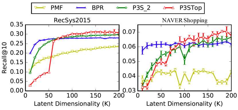
Figure 3: Recall@10 w.r.t. various $K$s on both datasets.

RQ4) Dimensionality Analysis. Figure 3 shows the impact of the number of latent dimensions $K$ on Recall for both datasets. While the performance of every method improved as $K$ increased, the performance improvements were more significant for P3S_2 and P3STop. We attribute this improvement to the fact that these methods need a larger model capacity than the rest of the methods because multiple relationships among itemsets are considered.

Self-information	BPR	P3STop
RecSys2015	8.8930	9.3439
NAVER Shopping	8.4382	10.0342

Table 6: Mean self-information of top-10 recommended items on both datasets.

RQ5) Preserving the novelty of recommendation. While it is important to provide accurate recommendations to users, another aspect of a successful recommender system that should not be neglected is the novelty of recommendations, as accuracy alone does not always result in user satisfaction [19]. In this respect, we compare the self-information (Equation 14 of top-10 recommended items of BPR with those of P3STop in Table 6. We observe that P3STop not only provides accurate recommendations compared with BPR, but also novel recommendations. We argue that this is mainly due to the fact that click records help reduce the dependence on the item popularity.

6 Related Work

6.1 Recommender Systems with Implicit Feedback

Although explicit feedback, such as rating, is a valuable source of information that reveals user preferences, it is difficult to obtain a large quantity of such data. Hence, the vast majority of work has focused on eliciting user preferences from implicit feedback such as bookmarks [58], item purchases [41, 10], and TV channel tuning history [33]. These methods adopted the MF technique to model the preference of users on items [18]. Specifically, Hu et al.  proposed WMF that [15] introduced the concept of confidence to measure the influence of observed items and unobserved items on users’ preferences. Later, various sampling strategies to generate negative examples from unobserved items were proposed [33, 11, 40]. Moreover, several pairwise learning-to-rank methods [41, 34, 54, 22] based on pairwise comparisons between observed items and unobserved items have been proposed. However, all the aforementioned methods are based on the AMAN assumption or predefined heuristic weights, which limits further performance improvement.

To cope with the aforementioned challenges, users’ social network information has been leveraged. For example, a method introduced by Zhao et al.  assigned higher ranks to the items that a user’s friends prefer than to the items that neither he nor his friends prefer [58]. This work was extended by Wang et al. [52], who introduced a method that categorizes unobserved items into three groups regarding users’ strong and weak ties with other users. However, these methods are only applicable when users’ social network information is available, which is usually not the case for most e-commerce stores. Various other methods that incorporate side information for solving the data sparsity issue of implicit feedback have been proposed: review text [51], item image [10] and temporal information [42]. However, this line of research is not directly related to our proposed method in that ours does not consider any side information. Moreover, dwell time [55] can be used to emphasize more reliable clicks, however, we argue that dwell time is a type of “temporal” side information that cannot be readily obtained. Lastly, Parra et al.  [35] proposed a parametric model to map implicit feedback to explicit feedback under the assumption that there is some correlation between implicit and explicit feedback. However, it requires a minimal amount of explicit feedback, whereas ours entirely resort to implicit feedback. Finally, as alternative approach for the same problem, we could think of feature engineering–based methods. Feature engineering–based methods refer to methods that manually generate features regarding the users and items. However, the generation of features is domain-specific [5], labor intensive and insufficient to uncover the underlying properties of data [49].

6.2 Modeling User Behavior

With the advent of e-commerce, much work has been devoted to understanding behavior of online users [28, 6], and specifically to predicting purchase behaviors [24, 25]. As the former line of work, Lo et al.  [28] studied user activity and purchasing behaviors that vary over time, especially focusing on user purchasing intent. Most recently, Cheng et al.  [6] extended Lo et al. ’s work [28] by generalizing their analysis on characterizing the relationship between a user’s intent and his behavior. Our goal is different in that we focus on predicting users’ purchases, rather than predicting users’ various intents from their online behaviors. Meanwhile, as the latter line of work, given user demographics and implicit feedback including click record and purchase record, Liu et al.  [25] proposed an ensemble method to predict which customers would return to the same merchant within six months period. They formulated the problem as a classification task and trained various classification methods. While similarly using both purchase record and click record, our task is different in that we aim to predict items that users will purchase rather than to predict repeat buyers. Moreover, Li et al.  [24] proposed a MF–based method that predicts the conversion response of users in display advertising, the goal of which inherently differs from our task.

6.3 Optimizing the Accuracy at the Top

Considering that users are mainly interested in the top-ranked items [1], optimizing for the accuracy near the top is of great importance in practice. Thanks to the success of the above approaches in general ranking tasks [31, 17, 44], they have been recently adopted in the field of recommender systems. Weimer et al.  proposed CoFiRank [53], which directly optimizes Normalized Discounted Cumulative Gain (NDCG) by minimizing its convex upper bound. Later, Shi et al.  proposed CLiMF [46], xCLiMF [48], and GAPfm [47], which optimize mean reciprocal rank, expected reciprocal rank and graded average precision, respectively. Among these methods, CLiMF is based on implicit feedback, whereas others are based on explicit feedback, and thus we compared our proposed method with CLiMF in our experiments in Section 5. Furthermore, Christakopoulou and Banerjee proposed PushCR, which applies p-norm push, infinite push and reverse-height push [44] to a collaborative ranking task in which the ranking loss focuses on the accuracy of the top-ranked items for each user [7]. Hu and Li recently proposed DCR, which focuses on the accuracy at the top by modeling user ratings based on an ordinal classification framework [14]. Lastly, Forsati et al.  [9] and Rafailidis and Crestani [38] incorporated user social network data as side information to enhance the accuracy at the top. However, these methods cannot be directly compared with ours because 1) PushCR and DCR consider explicit feedback, whereas ours is solely based on implicit feedback, and 2) the latter works incorporate side information related to users, whereas ours does not.

6.4 Position Bias of Click Models

Position bias is a fundamental problem pertaining to click records, where users tend to click on higher ranked items regardless of their relevance [43, 4]. To tackle the position bias issue for CTR prediction, previous click models assume that the click probability depends on the probability of examining a position, and the relevance of the document displayed at that position. However, we focus on purchase prediction rather than CTR prediction; we aim to overcome the data sparsity of purchase records by leveraging their relationships with click records. Hence, the position bias in terms of click models is out of scope for our current work.

7 Conclusion & Future Work

In this paper, we introduced a framework that leverages users’ past click records to complement the missing user–item interactions of purchase records. To this end, we formulated various model assumptions that define the order of user preferences regarding the non-purchased items, and demonstrated that click records are indeed useful for purchase prediction. We then proposed a novel learning-to-rank method, P3STop, that is customized to be robust to relatively unreliable click records by particularly focusing on the accuracy of the top-ranked items. We conducted extensive experiments on two real-world e-commerce datasets and verified the benefit of our proposed method compared with the state-of-the-art baselines. We believe that our method is beneficial to any e-commerce stores, such as Amazon and eBay, which collect both purchase and click records.

For future work, we plan to extend our framework 1) to model the temporal and sequential information [37] of clicks and purchases by using Markov chain–based methods [42] or deep learning–based approaches such as recurrent neural networks [27, 57] and convolutional neural networks [26], 2) to incorporate side information related to users and items, such as user reviews and item images, to enhance the performance of the purchase prediction even further, and 3) to incorporate click count information for purchase prediction. Although the click counts are important when the candidate purchase items are clicked-but-not-purchased items, but not as important when the candidate purchase items are items neither clicked nor purchased (as in our setting). However, we think that it will be interesting to see how the click counts would help purchase prediction in our setting.

8 Acknowledgment

This research was supported by the Ministry of Science and ICT (MSIT), Korea, under the Information and Communication Technology (ICT) Consilience Creative program (IITP-2019-2011-1-00783) and (IITP-2018-0-00584) supervised by the Institute for Information & communications Technology Planning & Evaluation (IITP), and Basic Science Research Program through the National Research Foundation of Korea (NRF) funded by the MSIT (NRF-2017M3C4A7063570) and (NRF-2016R1E1A1A01942642).

References

References

- top [2014] Amazon.com Search Click-Through Rates By Position, 2014. URL http://trends.e-strategyblog.com/2014/11/19/amazon-com-search-click-through-rates-by-position/22261.
- Castells et al. [2011] P Castells, S Vargas, and J Wang. Novelty and diversity metrics for recommender systems: choice, discovery and relevance. In International Workshop on Diversity in Document Retrieval (DDR 2011) at the 33rd European Conference on Information Retrieval (ECIR 2011), 2011.
- Chen et al. [2017] Jingyuan Chen, Hanwang Zhang, Xiangnan He, Liqiang Nie, Wei Liu, and Tat-Seng Chua. Attentive collaborative filtering: Multimedia recommendation with item-and component-level attention. In Proceedings of the 40th International ACM SIGIR conference on Research and Development in Information Retrieval, pages 335–344. ACM, 2017.
- Chen and Yan [2012] Ye Chen and Tak W Yan. Position-normalized click prediction in search advertising. In Proceedings of the 18th ACM SIGKDD international conference on Knowledge discovery and data mining, pages 795–803. ACM, 2012.
- Cheng et al. [2016] Heng-Tze Cheng, Levent Koc, Jeremiah Harmsen, Tal Shaked, Tushar Chandra, Hrishi Aradhye, Glen Anderson, Greg Corrado, Wei Chai, Mustafa Ispir, et al. Wide & deep learning for recommender systems. In Proceedings of the 1st workshop on deep learning for recommender systems, pages 7–10. ACM, 2016.
- Cheng et al. [2017] Justin Cheng, Caroline Lo, and Jure Leskovec. Predicting intent using activity logs: How goal specificity and temporal range affect user behavior. In Proceedings of the 26th International Conference on World Wide Web Companion, pages 593–601. International World Wide Web Conferences Steering Committee, 2017.
- Christakopoulou and Banerjee [2015] Konstantina Christakopoulou and Arindam Banerjee. Collaborative ranking with a push at the top. In Proceedings of the 24th International Conference on World Wide Web, pages 205–215. International World Wide Web Conferences Steering Committee, 2015.
- Donkers et al. [2017] Tim Donkers, Benedikt Loepp, and Jürgen Ziegler. Sequential user-based recurrent neural network recommendations. In Proceedings of the Eleventh ACM Conference on Recommender Systems, pages 152–160. ACM, 2017.
- Forsati et al. [2015] Rana Forsati, Iman Barjasteh, Farzan Masrour, Abdol-Hossein Esfahanian, and Hayder Radha. Pushtrust: An efficient recommendation algorithm by leveraging trust and distrust relations. In Proceedings of the 9th ACM Conference on Recommender Systems, pages 51–58. ACM, 2015.
- He and McAuley [2016] Ruining He and Julian McAuley. Vbpr: Visual bayesian personalized ranking from implicit feedback. In AAAI, pages 144–150, 2016.
- He et al. [2016] Xiangnan He, Hanwang Zhang, Min-Yen Kan, and Tat-Seng Chua. Fast matrix factorization for online recommendation with implicit feedback. In Proceedings of the 39th International ACM SIGIR conference on Research and Development in Information Retrieval, pages 549–558. ACM, 2016.
- He et al. [2017] Xiangnan He, Lizi Liao, Hanwang Zhang, Liqiang Nie, Xia Hu, and Tat-Seng Chua. Neural collaborative filtering. In Proceedings of the 26th International Conference on World Wide Web, pages 173–182. International World Wide Web Conferences Steering Committee, 2017.
- Hidasi et al. [2015] Balázs Hidasi, Alexandros Karatzoglou, Linas Baltrunas, and Domonkos Tikk. Session-based recommendations with recurrent neural networks. arXiv preprint arXiv:1511.06939, 2015.
- Hu and Li [2017] Jun Hu and Ping Li. Decoupled collaborative ranking. In Proceedings of the 26th International Conference on World Wide Web, pages 1321–1329. International World Wide Web Conferences Steering Committee, 2017.
- Hu et al. [2008] Yifan Hu, Yehuda Koren, and Chris Volinsky. Collaborative filtering for implicit feedback datasets. In Data Mining, 2008. ICDM’08. Eighth IEEE International Conference on, pages 263–272. Ieee, 2008.
- Kabbur et al. [2013] Santosh Kabbur, Xia Ning, and George Karypis. Fism: factored item similarity models for top-n recommender systems. In Proceedings of the 19th ACM SIGKDD international conference on Knowledge discovery and data mining, pages 659–667. ACM, 2013.
- Kar et al. [2015] Purushottam Kar, Harikrishna Narasimhan, and Prateek Jain. Surrogate functions for maximizing precision at the top. In International Conference on Machine Learning, pages 189–198, 2015.
- Koren et al. [2009] Yehuda Koren, Robert Bell, and Chris Volinsky. Matrix factorization techniques for recommender systems. Computer, 42(8), 2009.
- Kotkov et al. [2018] Denis Kotkov, Joseph A Konstan, Qian Zhao, and Jari Veijalainen. Investigating serendipity in recommender systems based on real user feedback. In Proceedings of the 33rd Annual ACM Symposium on Applied Computing, pages 1341–1350. ACM, 2018.
- Landin et al. [2019] Alfonso Landin, Daniel Valcarce, Javier Parapar, and Álvaro Barreiro. Prin: a probabilistic recommender with item priors and neural models. In European Conference on Information Retrieval, pages 133–147. Springer, 2019.
- Li et al. [2015a] Cheng Li, Yue Lu, Qiaozhu Mei, Dong Wang, and Sandeep Pandey. Click-through prediction for advertising in twitter timeline. In Proceedings of the 21th ACM SIGKDD International Conference on Knowledge Discovery and Data Mining, pages 1959–1968. ACM, 2015a.
- Li et al. [2016] Huayu Li, Richang Hong, Defu Lian, Zhiang Wu, Meng Wang, and Yong Ge. A relaxed ranking-based factor model for recommender system from implicit feedback. In Proceedings of the Twenty-Fifth International Joint Conference on Artificial Intelligence, pages 1683–1689. AAAI Press, 2016.
- Li et al. [2014] Nan Li, Rong Jin, and Zhi-Hua Zhou. Top rank optimization in linear time. In Advances in neural information processing systems, pages 1502–1510, 2014.
- Li et al. [2015b] Sheng Li, Jaya Kawale, and Yun Fu. Predicting user behavior in display advertising via dynamic collective matrix factorization. In Proceedings of the 38th International ACM SIGIR Conference on Research and Development in Information Retrieval, pages 875–878. ACM, 2015b.
- Liu et al. [2016a] Guimei Liu, Tam T Nguyen, Gang Zhao, Wei Zha, Jianbo Yang, Jianneng Cao, Min Wu, Peilin Zhao, and Wei Chen. Repeat buyer prediction for e-commerce. In Proceedings of the 22nd ACM SIGKDD International Conference on Knowledge Discovery and Data Mining, pages 155–164. ACM, 2016a.
- Liu et al. [2015] Qiang Liu, Feng Yu, Shu Wu, and Liang Wang. A convolutional click prediction model. In Proceedings of the 24th ACM International on Conference on Information and Knowledge Management, pages 1743–1746. ACM, 2015.
- Liu et al. [2016b] Qiang Liu, Shu Wu, Diyi Wang, Zhaokang Li, and Liang Wang. Context-aware sequential recommendation. In Data Mining (ICDM), 2016 IEEE 16th International Conference on, pages 1053–1058. IEEE, 2016b.
- Lo et al. [2016] Caroline Lo, Dan Frankowski, and Jure Leskovec. Understanding behaviors that lead to purchasing: A case study of pinterest. In Proceedings of the 22nd ACM SIGKDD International Conference on Knowledge Discovery and Data Mining, pages 531–540. ACM, 2016.
- McMahan et al. [2013] H Brendan McMahan, Gary Holt, David Sculley, Michael Young, Dietmar Ebner, Julian Grady, Lan Nie, Todd Phillips, Eugene Davydov, Daniel Golovin, et al. Ad click prediction: a view from the trenches. In Proceedings of the 19th ACM SIGKDD international conference on Knowledge discovery and data mining, pages 1222–1230. ACM, 2013.
- Mnih and Salakhutdinov [2008] Andriy Mnih and Ruslan R Salakhutdinov. Probabilistic matrix factorization. In Advances in neural information processing systems, pages 1257–1264, 2008.
- Narasimhan and Agarwal [2013] Harikrishna Narasimhan and Shivani Agarwal. A structural svm based approach for optimizing partial auc. In International Conference on Machine Learning, pages 516–524, 2013.
- Ning and Karypis [2011] Xia Ning and George Karypis. Slim: Sparse linear methods for top-n recommender systems. In 2011 IEEE 11th International Conference on Data Mining, pages 497–506. IEEE, 2011.
- Pan et al. [2008] Rong Pan, Yunhong Zhou, Bin Cao, Nathan N Liu, Rajan Lukose, Martin Scholz, and Qiang Yang. One-class collaborative filtering. In Data Mining, 2008. ICDM’08. Eighth IEEE International Conference on, pages 502–511. IEEE, 2008.
- Pan and Chen [2013] Weike Pan and Li Chen. Gbpr: Group preference based bayesian personalized ranking for one-class collaborative filtering. In IJCAI, volume 13, pages 2691–2697, 2013.
- Parra et al. [2011] Denis Parra, Alexandros Karatzoglou, Xavier Amatriain, and Idil Yavuz. Implicit feedback recommendation via implicit-to-explicit ordinal logistic regression mapping. Proceedings of the CARS-2011, 2011.
- Paszke et al. [2017] Adam Paszke, Sam Gross, Soumith Chintala, Gregory Chanan, Edward Yang, Zachary DeVito, Zeming Lin, Alban Desmaison, Luca Antiga, and Adam Lerer. Automatic differentiation in pytorch. 2017.
- Quadrana et al. [2018] Massimo Quadrana, Paolo Cremonesi, and Dietmar Jannach. Sequence-aware recommender systems. ACM Computing Surveys (CSUR), 51(4):66, 2018.
- Rafailidis and Crestani [2016] Dimitrios Rafailidis and Fabio Crestani. Joint collaborative ranking with social relationships in top-n recommendation. In Proceedings of the 25th ACM International on Conference on Information and Knowledge Management, pages 1393–1402. ACM, 2016.
- Ren et al. [2018] Pengjie Ren, Zhumin Chen, Jing Li, Zhaochun Ren, Jun Ma, and Maarten de Rijke. Repeatnet: A repeat aware neural recommendation machine for session-based recommendation. arXiv preprint arXiv:1812.02646, 2018.
- Rendle and Freudenthaler [2014] Steffen Rendle and Christoph Freudenthaler. Improving pairwise learning for item recommendation from implicit feedback. In Proceedings of the 7th ACM international conference on Web search and data mining, pages 273–282. ACM, 2014.
- Rendle et al. [2009] Steffen Rendle, Christoph Freudenthaler, Zeno Gantner, and Lars Schmidt-Thieme. Bpr: Bayesian personalized ranking from implicit feedback. In Proceedings of the twenty-fifth conference on uncertainty in artificial intelligence, pages 452–461. AUAI Press, 2009.
- Rendle et al. [2010] Steffen Rendle, Christoph Freudenthaler, and Lars Schmidt-Thieme. Factorizing personalized markov chains for next-basket recommendation. In Proceedings of the 19th international conference on World wide web, pages 811–820. ACM, 2010.
- Richardson et al. [2007] Matthew Richardson, Ewa Dominowska, and Robert Ragno. Predicting clicks: estimating the click-through rate for new ads. In Proceedings of the 16th international conference on World Wide Web, pages 521–530. ACM, 2007.
- Rudin [2009] Cynthia Rudin. The p-norm push: A simple convex ranking algorithm that concentrates at the top of the list. Journal of Machine Learning Research, 10(Oct):2233–2271, 2009.
- Sarwar et al. [2001] Badrul Sarwar, George Karypis, Joseph Konstan, and John Riedl. Item-based collaborative filtering recommendation algorithms. In Proceedings of the 10th international conference on World Wide Web, pages 285–295. ACM, 2001.
- Shi et al. [2012] Yue Shi, Alexandros Karatzoglou, Linas Baltrunas, Martha Larson, Nuria Oliver, and Alan Hanjalic. Climf: learning to maximize reciprocal rank with collaborative less-is-more filtering. In Proceedings of the sixth ACM conference on Recommender systems, pages 139–146. ACM, 2012.
- Shi et al. [2013a] Yue Shi, Alexandros Karatzoglou, Linas Baltrunas, Martha Larson, and Alan Hanjalic. Gapfm: Optimal top-n recommendations for graded relevance domains. In Proceedings of the 22nd ACM international conference on Conference on information & knowledge management, pages 2261–2266. ACM, 2013a.
- Shi et al. [2013b] Yue Shi, Alexandros Karatzoglou, Linas Baltrunas, Martha Larson, and Alan Hanjalic. xclimf: optimizing expected reciprocal rank for data with multiple levels of relevance. In Proceedings of the 7th ACM conference on Recommender systems, pages 431–434. ACM, 2013b.
- Sun et al. [2015] Yaming Sun, Lei Lin, Duyu Tang, Nan Yang, Zhenzhou Ji, and Xiaolong Wang. Modeling mention, context and entity with neural networks for entity disambiguation. In Twenty-Fourth International Joint Conference on Artificial Intelligence, 2015.
- Valcarce et al. [2018] Daniel Valcarce, Alejandro Bellogín, Javier Parapar, and Pablo Castells. On the robustness and discriminative power of information retrieval metrics for top-n recommendation. In Proceedings of the 12th ACM Conference on Recommender Systems, pages 260–268. ACM, 2018.
- Wang and Blei [2011] Chong Wang and David M Blei. Collaborative topic modeling for recommending scientific articles. In Proceedings of the 17th ACM SIGKDD international conference on Knowledge discovery and data mining, pages 448–456. ACM, 2011.
- Wang et al. [2016] Xin Wang, Wei Lu, Martin Ester, Can Wang, and Chun Chen. Social recommendation with strong and weak ties. In Proceedings of the 25th ACM International on Conference on Information and Knowledge Management, pages 5–14. ACM, 2016.
- Weimer et al. [2008] Markus Weimer, Alexandros Karatzoglou, Quoc V Le, and Alex J Smola. Cofi rank-maximum margin matrix factorization for collaborative ranking. In Advances in neural information processing systems, pages 1593–1600, 2008.
- Weston et al. [2011] Jason Weston, Samy Bengio, and Nicolas Usunier. Wsabie: scaling up to large vocabulary image annotation. In Proceedings of the Twenty-Second international joint conference on Artificial Intelligence-Volume Volume Three, pages 2764–2770. AAAI Press, 2011.
- Yi et al. [2014] Xing Yi, Liangjie Hong, Erheng Zhong, Nanthan Nan Liu, and Suju Rajan. Beyond clicks: dwell time for personalization. In Proceedings of the 8th ACM Conference on Recommender systems, pages 113–120. ACM, 2014.
- Zhang et al. [2018] Yongfeng Zhang, Xu Chen, Qingyao Ai, Liu Yang, and W Bruce Croft. Towards conversational search and recommendation: System ask, user respond. In Proceedings of the 27th ACM International Conference on Information and Knowledge Management, pages 177–186. ACM, 2018.
- Zhang et al. [2014] Yuyu Zhang, Hanjun Dai, Chang Xu, Jun Feng, Taifeng Wang, Jiang Bian, Bin Wang, and Tie-Yan Liu. Sequential click prediction for sponsored search with recurrent neural networks. In AAAI, volume 14, pages 1369–1375, 2014.
- Zhao et al. [2014] Tong Zhao, Julian McAuley, and Irwin King. Leveraging social connections to improve personalized ranking for collaborative filtering. In Proceedings of the 23rd ACM International Conference on Conference on Information and Knowledge Management, pages 261–270. ACM, 2014.
- Zhou et al. [2010] Tao Zhou, Zoltán Kuscsik, Jian-Guo Liu, Matúš Medo, Joseph Rushton Wakeling, and Yi-Cheng Zhang. Solving the apparent diversity-accuracy dilemma of recommender systems. Proceedings of the National Academy of Sciences, 107(10):4511–4515, 2010.
- Zhu et al. [2010] Zeyuan Allen Zhu, Weizhu Chen, Tom Minka, Chenguang Zhu, and Zheng Chen. A novel click model and its applications to online advertising. In Proceedings of the third ACM international conference on Web search and data mining, pages 321–330. ACM, 2010.