The dynamic three-dimensional Anderson localization of optical fields in active percolating systems

Abstract

We study three-dimensional optical Anderson localization in medium with a percolating disorder, where the percolating clusters are filled by the light nanoemitters in the excited state. The peculiarity of situation is that in such materials the field clusters join a fractal radiating system where the light is both emitted and scattered by the inhomogeneity of clusters. Our numerical FDTD simulations found that in this nonlinear compound the number of localized field bunches drastically increases after the lasing starts. At longer times the bunches leave nonlinear percolating structure and are radiated from the medium. Monitoring the output of system allows to observe experimentally such dynamic localized bunches in three-dimensional setup.

Introduction. Disordered photonic materials can diffuse and localize light through random multiple scattering that leads to formation of the electromagnetic modes depending on the structural correlations, scattering strength, and dimensionality of the system Riboli:2014 , Vinck:2011 , Sheng:2010 , Wang:2011 , jendrzejewski:2012 , Segev:2013a , Wiersma:2013a . The Anderson localization was predicted as a non-interacting linear interference effect anderson:1958 . However, in real systems the non-negligible interactions between light and medium can take place. Therefore important aspect of the optical localization is the interplay between nonlinear interactions and linear Anderson effect Segev:2013a . Nonlinear interactions appear in optics, due to nonlinear responses of a disordered medium that normally gives rise to indirect interactions between the photons through various mechanisms. In case of classical waves the localization can be interpreted as interference between the various amplitudes associated with the scattering paths of optical waves propagating among the diffusers. The study for Anderson transition in 3-D optical systems still has not been conclusive despite considerable efforts. The localization transition may be difficult to reach for the light waves due to various effects in dense disordered media required to achieve strong scattering [see Skipetrov:2016a and references therein]. The experimental observation of optical Anderson localization Sanli:2009a just below the Anderson transition in 3D disordered medium shows strong fluctuations of the wave function that leads to nontrivial length-scale dependence of the intensity distribution (multifractality).

Here we study the optical Anderson localization in 3D percolating disorder, where the percolating clusters are filled by the light nanoemitters in the excited state. The peculiarity of situation is that in such materials the field clusters join a fractal nonlinear radiating system where the light is both emitted and scattered by the inhomogeneity of clusters. Such system may be suggested as an extension to 3D optical case the localization released in one-dimensional waveguide in the presence of a controlled disorder Billy:2008a . In 3D disordered percolating systems the optical transport was observed Burlak:2009a and also it is found that the random lasing assisted by nanoemitters incorporated into such a disordered structure can occur burlak:2015 . The system with spanning clusters produces a global percolation that results in qualitatively modification of its spatial properties. One can argues that already in a vicinity of the percolating phase transition the fractal dimension of such system $D_{H}\simeq 2.54$ considerably differs from the dimension of the embedded space $D=3$ (multifractality). The crucial question is whether the optical Anderson localization can be achieved for a non-integer dimension case with a fractal (Hausdorff) dimension of $D_{H}<3$, where the strong randomness for properties of the system is expected. In this paper we show that the dynamic field localization can arise in such 3D active fractal percolation system. To the best of our knowledge, the dynamic 3D Anderson localization assisted by fractal disordered inhomogeneity is discussed here for the first time.

Basic equations. The percolation normally refers to the leakage of fluid or gas through the porous materials. In this paper we consider that the percolating clusters are filled by gaseous light nanoemitters in the excited state. A typical incipient percolation cluster has a dendrite shape. From Fig. 1 (a) we observe that such a system consists of two essentially different areas. In the first region (in the vicinity of the entrance shown by arrow) there is a strong concentration of percolation clusters, which may lead to accumulation of the nonlinear field effects and the lasing. In the other part, the concentration of percolation clusters is small, so the disorder of medium is lower. We study the emission of electromagnetic energy from a cubical sample $(x,y,z)\in[0,l_{0}]$ in 3D medium with a percolating disorder, where the percolating clusters are filled by the light nanoemitters in the excited state. The output flux of energy can be written as $I=\oint_{S}(\mathbf{K}\cdot\mathbf{n})dS=I_{x}+I_{y}+I_{z}$, where $\mathbf{K}$ is the Pointing vector, $\mathbf{n}$ is the normal unit vector to the surface $S$ of cube, and $I_{x,y,z}$ indicate the fluxes from two faces of the cube perpendicular to a particular direction. To find the emission from the system we solve numerically the following equations that couple the polarization density $\mathbf{P}$, the electric field $\mathbf{E}$, and occupations of the levels of emitters $N_{i}$ Siegman:1986

$$\frac{\partial^{2}\mathbf{P}}{\partial t^{2}}+\Delta\omega_{a}\frac{\partial\mathbf{P}}{\partial t}+{\omega_{a}^{2}}\mathbf{P}=\frac{6\pi\varepsilon_{0}c^{3}}{\tau_{21}\omega_{a}^{2}}(N_{1}-N_{2})\mathbf{E,}$$

       (1)

here $\Delta\omega_{a}=\tau_{21}^{-1}+2T_{2}^{-1}$, where $T_{2}$ is the mean time between dephasing events, $\tau_{21}$ is the decay time from the second atomic level to the first one, and $\omega_{a}$ is the frequency of radiation. The electric and magnetic fields, $\mathbf{E}$ and $\mathbf{H}$, and the current $\mathbf{j}=\partial\mathbf{P}/\partial t$ are found from the Maxwell equations, together with the equations for the densities $N_{i}(\mathbf{r},t)$ of atoms residing in $i-$th level, see Soukoulis:2000 and references therein. An external source excites emitters from the ground level ($i=0$) to third level at a certain rate $A_{r}$ , which is proportional to the pumping intensity in experiments. After a short lifetime $\tau_{32}$, the emitters transfer nonradiatively to the second level. The second level and the first level are the upper and the lower lasing levels, respectively. Emitters can decay from the upper to the lower level by both spontaneous and stimulated emission, and $(\mathbf{j}\cdot\mathbf{E})/\hbar\omega_{a}$ is the stimulated radiation rate. Finally, emitters can decay nonradiatively from the first level back to the ground level. The lifetimes and energies of upper and lower lasing levels are $\tau_{21}$, $E_{2}$ and $\tau_{10}$, $E_{1}$, respectively. The individual frequency of radiation of each emitter is then $\omega_{a}=\left(E_{2}-E_{1}\right)/\hbar$, and $\hbar$ is Planck’s constant.

Numerics. In our calculations we considered the gain medium with parameters close $GaN$ powder, similar to Ref. expt . The lasing frequency $\omega_{a}$ is $2\pi\times 3\times 10^{13}\,Hz$, the lifetimes are $\tau_{32}=0.3\,ps$, $\tau_{10}=1.6\,ps$, $\tau_{21}=16.6\,ps$, and the dephasing time is $T_{2}=0.0218\,ps$. The percolating cluster has been generated inside the cube of $l_{0}=1\,\mu m$ edge having $L^{3}$ nodes, with $L=100$ (see Fig.1 (a)) that was sufficient to simulate the percolating structure Burlak:2009a . Each node is supposed to indicate the position of many emitters, with the total concentration of emitters inside the percolation cluster being $N=N_{0}+N_{1}+N_{2}+N_{3}=3.3\times 10^{24}\,m^{-3}$. The initial (at $t=0$) values of densities $N_{0}(0)=0.001\,N$, $N_{1}(0)=0.002\,N$, $N_{2}(0)=0.002\,N$, and $N_{3}(0)=0.995\,N$ are used. The dielectric permittivity of a host material is $n=2.2$ that is close to the typical values for ceramics $Lu_{3}Al_{5}O_{12}$, $SrTiO_{3}$, $ZrO_{2}$, see review Sanghera:2012 . The result of simulations shown in Fig. 1 (b) obtained for cw pumping given by $A_{r}=10^{7}\,s^{-1}$. At this pumping the simulations show the formation a well-defined lasing for $t>t_{s}$, and we refer $t_{s}$ as the lasing start time. To simulate the noise in our system the initial seed for the electromagnetic field has been created with random phases at each node. In what follows it is used dimensionless time $t$ renormalized as $t\rightarrow tc/l_{0}$,where $c$ is the light velocity in vacuum.

Briefly, the strategy of our simulations consists in the following: (i) Calculating the geometry of the spanning percolating cluster, (ii) Calculating the photon field $\mathbf{E}$ generated by emitters incorporated in spanning cluster with the use of finite-difference time-domain (FDTD) technique AllenTaflove:2005a , and (iii) Solution of nonlinear dynamic coupled equations for field, polarization $\mathbf{P}$ and the occupation numbers $N_{i}$ for all the emitters in 3D system.

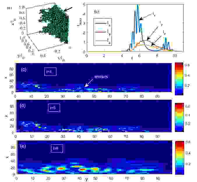
Figure 1: (Color online.) (a) Typical spatial structure of the incipient percolating cluster near the percolation threshold in the cube $l_{0}\times l_{0}\times l_{0}$. (b) The dynamics of lasing (the critical lasing time is $t_{c}=5$), where the field fluxes $I_{xyz}$ in the $xyz$ -directions of the system are displayed; (c) The normalized fields in the central intersection $xy$ of 3D system for various times closely to the critical time at: (c) $t=4<t_{c}$, and (d) $t=5=t_{c}$. In such situation only narrow point-like fields generated by random emitters are observed. For longer time at $t=6>t_{c}$ (e) the field bunches having smooth localized shape and large amplitudes arise already beyond the emitter peaks. Hence the lasing in percolating disordered system will stimulate the localization of emitted field.

We use here the extended 3D percolating model that allows the empty percolating voids to have a small random-valued 3D shift from the reference grid. We use the percolating probability $p=0.4$ that is slightly less of corresponding threshold $0.415$ for such extended model. Fig.1 (a) shows the typical spatial structure of the incipient percolating cluster in the cube $l_{0}\times l_{0}\times l_{0}$ corresponding to the numerical grid with $L\times L\times L$, $L=100$ nodes. Fig.1 (b) displays the dynamics of optical lasing generated by exited emitters in percolating medium with intensities $I_{x,y,z}$ through the sides of 3D sample. The normalized field amplitudes $E_{x}$ in the central intersection ($x,y=L/2$) of 3D percolating system at different times nearly of the initial time of laser generation ($t=4,5,6$) are shown in Fig.1, panels (c), (d), and (e). Fig.1 (c) shows the fields distribution before the lasing starts. In this case the field amplitudes are small, one can observe only narrow point-like fields (indicated by arrow) generated by random emitters in percolating cluster. At larger time $t=5$ (see Fig.1, panel (d)) the laser generation starts that leads to increase of the field amplitudes in the emitter positions, however the radiation field still is small. But for $t=6$ (peak of lasing, see Fig.1, (b), (e)) we observe the appearance of intensive radiating light beyond the emitter peaks.

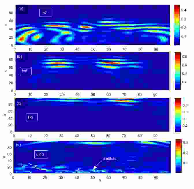
Figure 2: (Color online.) The field distribution for longer times. Panels (a) $t=7$ and (b) $t=8$ show the dynamic states (coupled to emitters) when the light bunches begin to migrate from the random emitter area. (That corresponds to lasing evolution in Fig.1 (b) for the interval $t=7,8$ when in the system after emission the accumulation of energy occurs. Panels (c) $t=9$ and (d) $t=10$ show that for long time the optical bunches reach the output of system, and at $t=10$ (d) the localized light is radiated to surrounding space.

Fig.2 shows the developed field distribution for larger times: $t=7,8,9,10$, when the advanced lasing occurs. From this figure one can determine $t=t_{D}$ as a maximum dwell time such that for $t\leq t_{D}$ the dynamic bunches are still formed in all the nonlinear and disordered part of system from $x=0$ up to $x=L/2$ and for $t>t_{D}$ the fiel bunches are concentrated at $x>L/2$. Figures 2 (a) and (b) show the nonlinear dynamics at $t=7$ and $t=8$ when well-formed field bunches with high amplitude start to leave the random emitter area . This corresponds to field evolution in Fig.1 (b) for $t=7,8$ when the system after emission is in the state of the energy accumulation. Fig.2 (c), (d) show that for longer time the field bunches move to output of system; at $t=9$ they are closely to the output and first front starts to leave the system. Moreover, we observe from Fig.2 (d) that at $t=10$ the bunches have been radiated away the system such that the field tails have quite small amplitude, therefore the points-like emitter fields (close to the input) are seen in this amplitude scale. We observe that for the used parameters the dwell time is $t_{D}\approx 7$.

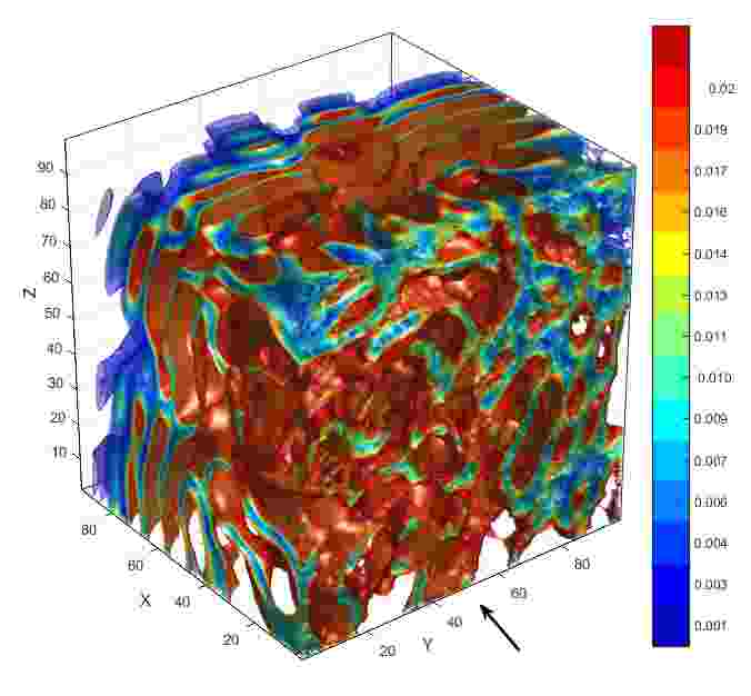
Figure 3: (Color online.) The isosurface of 3D emitted field shown in Fig. 2 (a) for time $t=7$. We observe that the field has indented shape of light structures with bunches and worm-holes due to the fractality of radiated system.

Fig.2 exhibits the fields in central intersection of 3D system. However, since the clusters have nonuniform fractal structure it is more informative to explore the shape of fields in total 3D volume. Fig. 3 displays the isosurface of field in 3D system shown in Fig. 2 (a) for time $t=t_{D}=7$ when the optical fields have already well-established structure. We observe from Fig. 3 that in general field consists of bunches having different amplitudes and shapes. The bunches are separated by 3D worm-holes (with small field) having irregular shapes that emerge due to the non-integer fractal dimension ($D_{H}=2.54$) of percolating clusters.

Localization. In the above the properties of generated field bunches were analyzed in general. In what follows we study the dynamics and structure of localized fields confined in the light bunches. A field (quasi-spherical) bunch will be mentioned as a bounded 3D domain where field Ei in every layer i is a decreasing function $Ei>Ei+1$ $(i\in 0,1,\ldots p-1$) from center to periphery that leads to $E_{0}>E_{1}>\ldots>E_{p}>0$. Such domain (bunch) have two parameters: radius $p$ and the field value in the center $E_{0}=E_{max}$. [More detailed approaches in such 3D localization problem require too large amount of computer resources.]

Figure 4: (Color online.) The positions and shapes of some localized field bunches with highest (normalized) amplitudes in center $E_{max}$ and largest radius $p$ for $t=t_{D}=7$ (see Fig. 2 (a)) situated in different points of 3D system: (a) $E_{max}=0.98$ at $x=14,y=18,z=73,p=5$; (b) $E_{max}=0.96$ at $x=13,y=26,z=18,p=5$; (c) $E_{max}=0.73$ at $x=15,y=41,z=64,p=4$; (d) $E_{max}=0.74$ at $x=15,y=41,z=64,p=4$; (e) $E_{max}=0.5$ at $x=73,y=20,z=32,p=5$ , and (f) $E_{max}=0.55$ at $x=18,y=35,z=21,p=5$. In general case the bunches are situated in random positions due to disordered radiated emitters and the fractality of percolating clusters.

From Fig. 4 one observes for time $t=t_{D}=7$ the structure of some localized field with large amplitudes $E_{max}$ and characteristic radius $p$. The centers of such objects are established in various points of 3D medium. Fig. 4 displays the isosurface of normalized fields for such items. In general the bunches are situated in variety points of 3D system, see Fig. 3 due to disordering positions of radiated emitters and the fractal shape of the percolating clusters. As we observer from Fig. 4 all the bunches have well established localized shape.

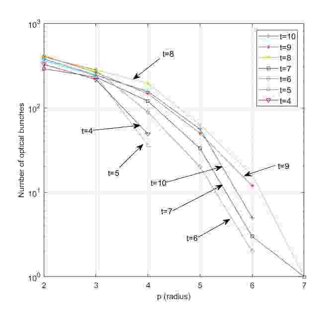
Figure 5: (Color online.) Dependence the number of optical bunches $N$ on the radius $p$ for various times $t=4,5,6,7,8,9,10$. We observe that $N$ with large radius $p$ drastically increments after $t>5$ when the lasing starts. At $t=t_{D}=7$ and $t=8$ it is generated the bunch with maximal characteristic radius $p=7$.

It is interesting to study the dependence of number of bunches at different times $t$ as function of radius $p$. Fig.5 shows such dependence for times $t=4,5,6,7,8,9,10$. We observe from Fig.5 that below the lasing threshold ($t\leq 5$, see Fig. 1 (b)) there are large number of bunches with small radius $p$. Most of them correspond to narrow point-like fields generated in vicinity of random light emitters (see Fig. 1 (c)). However, as one can see from Fig.5, after the lasing starts (since $t>5$) the number of optical bunches with large radius $p$ drastically increments. Besides, Fig. 2 displays that such bunches (wth large $p$) are situated mainly beyond the percolating area. Moreover, as Fig. 2 shows such fields have well-localized shape (Fig. 4), they are not pinned to the static emitters and migrate to the output. That allows indicating such dynamic bunches as 3D zones of optical Anderson localization arisen by the active disordered fractal percolating clusters.

Finally it is especially interesting to study the dependence amount of bunches at different times $t$ as function of radius $p$. Fig.5 shows such dependence for times $t=4,5,6,7,8,9,10$. We observe from Fig.5 that below the lasing threshold ($t\leq 5$, see Fig. 1 (b)) there are a lot of field peaks with small radius $p$. Most of them correspond to narrow point-like fields generated by random light emitters (see Fig. 1 (c)). However, as one can see from Fig.5, after the lasing starts (since $t>5$) the number of optical bunches with large radius $p$ drastically increments. Besides, Fig. 2 displays that such bunches (with large $p$) are situated mainly beyond the percolating area. Moreover, as Fig. 2 shows such fields have well-localized shape (Fig. 4), they longer are not pinned to the static emitters and they migrate to the output of system. That allows indicating such dynamic bunches as 3D zones of optical Anderson localization arisen by the active fractal percolating clusters.

Conclusion. We have shown that dynamic 3D optical Anderson localization can arise in medium with percolating disorder when the percolating clusters are filled by the light nanoemitters in the excited state. In such materials the field emitters in clusters create a fractal radiating system, where the field is not only emitted, but also scattered by the boundaries of clusters. Our 3D simulations have found that in such nonlinear compound the amount of localized field bunches drastically increases after the optical lasing starts. At longer times all the bunches leave nonlinear percolating structure and are radiated from the medium.

References

- (1) F. Riboli, N. Caselli, S. Vignolini, et.al., Nature Materials, Vol. 13 (7), pp. 720-725 (2014).
- (2) K. Vynck, M. Burresi, F. Riboli, D. S. Wiersma, Nature Materials, vol. 11, pp. 1017–1022 (2012).
- (3) P. Sheng, Introduction to Wave Scattering, Localization and Mesoscopic phenomena (Springer, 2010), 2nd ed.,.
- (4) J. Wang and A. Z. Genack, Nature 471, 345 (2011).
- (5) F. Jendrzejewski, A. Bernard, K. Muller, P. Cheinet, et. al., Nature Physics 8, 398–403 (2012).
- (6) M. Segev, Y. Silberberg, D. N. Christodoulides, Nature Photonics 7, 197–204 (2013)
- (7) D. S. Wiersma, Nature Photonics. 7, 3, 188-196 (2013).
- (8) P. W. Anderson, Phys. Rev.,109, 1492 (1958).
- (9) Skipetrov, S.E., Phys. Rev. B. 94, 6, 064202 (2016).
- (10) Sanli Faez, Anatoliy Strybulevych, John H. Page, Ad Lagendijk, and Bart A. van Tiggelen, Phys. Rev. Lett. 103, 155703 (2009).
- (11) G. Burlak, M. Vlasova, P. A. Marquez Aguilar, et.al., Opt. Commun. 282, 2850 (2009).
- (12) G. Burlak and Y. G. Rubo, Phys. Rev. A, 92, 013812, 2015.
- (13) J. Sanghera, W. Kim, G. Villalobos, et.al., Materials 5, 258 (2012).
- (14) A. E. Siegman, Lasers (Mill Valley, California, 1986).
- (15) Xunya Jiang and C. M. Soukoulis, Phys. Rev. Lett. 85, 70 (2000).
- (16) C. Conti and A. Fratalocchi, Nat. Phys. 4, 794 (2008).
- (17) A. Taflove and S. C. Hagness, Computational Electrodynamics: The Finite-Difference Time-Domain Method (Artech House Publishers, 3rd edition, 2005).
- (18) H. Cao, Y. G. Zhao, S. T. Ho, E. W. Seelig, Q. H. Wang, and R. P. H. Chang, Phys. Rev. Lett. 82, 2278 (1999).
- (19) J. Billy, V. Josse, Z. Zuo, et.al. Nature 453, 891-894 (2008)