Topological Interplay between Knots and Entangled Vortex-Membranes

Abstract

In this paper, the Kelvin wave and knot dynamics are studied on three dimensional smoothly deformed entangled vortex-membranes in five dimensional space. Owing to the existence of local Lorentz invariance and diffeomorphism invariance, in continuum limit gravity becomes an emergent phenomenon on 3+1 dimensional zero-lattice (a lattice of projected zeroes): On the one hand, the deformed zero-lattice can be denoted by curved space-time for knots; on the other hand, the knots as topological defect of 3+1 dimensional zero-lattice indicates matter may curve space-time. This work would help researchers to understand the mystery in gravity.

I Introduction

A vortex (point-vortex, vortex-line, vortex-membrane) consists of the rotating motion of fluid around a common centerline. It is defined by the vorticity in the fluid, which measures the rate of local fluid rotation. In three dimensional (3D) superfluid (SF), the quantization of the vorticity manifests itself in the quantized circulation ${\displaystyle\oint}\mathbf{v}\cdot d\mathbf{l}=\frac{h}{m}$ where $h$ is Planck constant and $m$ is atom mass of SF. Vortex-lines can twist around its equilibrium position (common centerline) forming a transverse and circularly polarized wave (Kelvin wave)Thomson1880a ; Donnelly1991a . Because Kelvin waves are relevant to Kolmogorov-like turbulenceS95 ; V00 , a variety of approaches have been used to study this phenomenon. For two vortex-lines, owing to the interaction, the leapfrogging motion has been predicted in classical fluids from the works of Helmholtz and Kelvindys93 ; hic22 ; bor13 ; wac14 ; cap14 ; 1 . Another interesting issue is entanglement between two vortex-lines. In mathematics, vortex-line-entanglement can be characterized by knots with different linking numbers. The study of knotted vortex-lines and their dynamics has attracted scientists from diverse settings, including classical fluid dynamics and superfluid dynamicsKleckner2013 ; Hall2016 .

In the paperkou , the Kelvin wave and knot dynamics in high dimensional vortex-membranes were studied, including the leapfrogging motion and the entanglement between two vortex-membranes. A new theory - knot physics is developed to characterize the entanglement evolution of 3D leapfrogging vortex-membranes in five-dimensional (5D) inviscid incompressible fluid. According to knot physics, it is the 3D quantum Dirac model that describes the knot dynamics of leapfrogging vortex-membranes (we have called it knot-crystal, that is really plane Kelvin-waves with fixed wave-length). The knot physics may give a complete interpretation on quantum mechanics.

In this paper, we will study the Kelvin wave and knot dynamics on 3D deformed knot-crystal, particularly the topological interplay between knots and the lattice of projected zeroes (we call it zero-lattice). Owing to the existence of local Lorentz invariance and diffeomorphism invariance, the gravitational interaction emerges: On the one hand, the deformed zero-lattice can be denoted by curved space-time; on the other hand, the knots deform the zero-lattice that indicates matter may curve space-time (see below discussion).

The paper is organized as below. In Sec. II, we introduce the concept of ”zero-lattice” from projecting a knot-crystal. In addition, to characterize the entangled vortex-membranes, we introduce geometric space and winding space. In Sec. III, we derive the massive Dirac model in the vortex-representation of knot states on geomatric space and that on winding space. In Sec. IV, we consider the deformed knot-crystal as a background and map the problem onto Dirac fermions on a curved space-time. In Sec. V, the gravity in knot physics emerges as a topological interplay between zero-lattice and knots and the knot dynamics on deformed knot-crystal is described by Einstein’s general relativity. Finally, the conclusions are drawn in Sec. VI.

II Knot-crystal and the corresponding zero-lattice

II.1 Knot-crystal

Knot-crystal is a system of two periodically entangled vortex-membranes that is described by a special pure state of Kelvin waves with fixed wave length $\mathbf{Z}_{\mathrm{knot-crystal}}(\vec{x},t)$kou . In emergent quantum mechanics, we consider knot-crystal as a ground state for excited knot states, i.e.,

$$\mathbf{Z}_{\mathrm{knot-crystal}}(\vec{x},t)=\left(\begin{array}[c]{c}\mathrm{z}_{\mathrm{A}}(\vec{x},t)\\ \mathrm{z}_{\mathrm{B}}(\vec{x},t)\end{array}\right)\rightarrow\left|\text{{vacuum}}\right\rangle.$$ (1)

On the one hand, a knot is a piece of knot-crystal and becomes a topological excitation on it; On the other hand, a knot-crystal can be regarded as a composite system with multi-knot, each of which is described by same tensor state.

Because a knot-crystal is a plane Kelvin wave with fixed wave vector $k_{0}$, we can use the tensor representation to characterize knot-crystalskou ,

$$\mathbf{\vec{\Gamma}}_{\mathrm{knot-crystal}}^{I}=(\vec{n}_{\sigma}^{I}\mathbf{\sigma}^{I})\otimes(\vec{n}_{\tau}\mathbf{\tau}+\vec{1}\tau_{0})$$ (2)

where $\vec{1}=\left(\begin{array}[c]{cc}1&0\\ 0&1\end{array}\right)$ and $\mathbf{\sigma}^{I}$, $\mathbf{\tau}^{I}$ are $2\times 2$ Pauli matrices for helical and vortex degrees of freedom, respectively. For example, a particular knot-crystal is called SOC knot-crystal $\mathbf{Z}_{\mathrm{knot-crystal}}(\vec{x})$kou , of which the tensor state is given by

$$\left\langle\mathbf{\sigma}^{X}\otimes\vec{1}\right\rangle =\vec{n}_{\sigma}^{X}=(1,0,0),$$ (3)

$$\left\langle\mathbf{\sigma}^{Y}\otimes\vec{1}\right\rangle =\vec{n}_{\sigma}^{Y}=(0,1,0),$$

$$\left\langle\mathbf{\sigma}^{Z}\otimes\vec{1}\right\rangle =\vec{n}_{\sigma}^{Z}=(0,0,1).$$

For the SOC knot-crystal, along x-direction, the plane Kelvin wave becomes $\mathrm{z}(x)=\sqrt{2}r_{0}\cos(k_{0}\cdot x);$ along y-direction, the plane Kelvin wave becomes $\mathrm{z}(y)=\frac{1}{\sqrt{2}}r_{0}(e^{ik\cdot y}+ie^{-ik\cdot y});$ along z-direction, the plane Kelvin wave becomes $\mathrm{z}(z)=r_{0}e^{ik\cdot z}.$

For a knot-crystal, another important property is generalized spatial translation symmetry that is defined by the translation operation $\mathcal{T}(\Delta x^{I})=e^{i\cdot(\hat{k}_{0}^{I}\cdot\Delta x^{I})\cdot\mathbf{\vec{\Gamma}}_{\mathrm{knot-crystal}}^{I}}$

$$\mathbf{Z}(x^{I},t) \rightarrow\mathcal{T}(\Delta x^{I})\mathbf{Z}(x^{i},t)$$

$$=e^{i\cdot(\hat{k}_{0}^{I}\cdot\Delta x^{i})\cdot\mathbf{\vec{\Gamma}}_{\mathrm{knot-crystal}}^{I}}\mathbf{Z}(x^{i},t).$$ (4)

Here $\hat{k}^{I}$ is $-i\frac{d}{dx^{I}}$ ($I=x,y,z$). For example, for the knot states on 3D SOC knot-crystal, the translation operation along $x^{I}$-direction becomes

$$\mathcal{T}(\Delta x^{I})=e^{i(\hat{k}^{I}\cdot\Delta x^{I})\cdot(\sigma^{I}\otimes\vec{1})}.$$ (5)

II.2 Winding space and geometric space

For a knot-crystal, we can study it properties on a 3D space ($x,y,z$). In the following part, we call the space of ($x,y,z$) geometric space. According to the generalized spatial translation symmetry, each spatial point ($x,y,z$) in geometric space corresponds to a point denoted by three winding angles $(\Phi_{x}(x),\Phi_{y}(y),\Phi_{z}(z))$ where $\Phi_{x^{I}}(x^{I})$ is the winding angle along $x^{I}$-direction. As a result, we may use the winding angles along different directions to denote a given point $\vec{\Phi}(\vec{x})=(\Phi_{x}(x),\Phi_{y}(y),\Phi_{z}(z)).$ We call the space of winding angles $(\Phi_{x}(x),\Phi_{y}(y),\Phi_{z}(z))$ winding space. See the illustration in Fig.1(d).

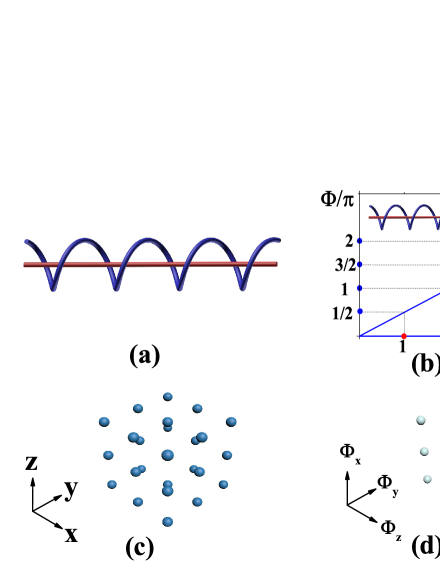
Figure 1: (a) An illustration of a 1D knot-crystal; (b) The relationship between winding angle $\Phi$ and coordinate position $x$. The red dots consist of a 1D zero-lattice in geometric space and the blue dots consist of a zero-lattice in winding space; (c) An illustration of a 3D uniform zero-lattice in geometric space; (d) An illustration of a 3D uniform zero-lattice in winding space.

For a 1D leapfrogging knot-crystal that describes two entangled vortex-lines with leapfrogging motion, the function is given by

$$\mathbf{Z(}\vec{x},t\mathbf{)}=r_{0}\left(\begin{array}[c]{c}\cos(\frac{\omega^{\ast}t}{2})\\ -i\sin(\frac{\omega^{\ast}t}{2})\end{array}\right)e^{i\frac{\pi}{a}x}e^{-i\omega_{0}t+i\omega^{\ast}t/2},$$ (6)

where $\omega^{\ast}$ is angular frequency of leapfrogging motion. For the 1D $\sigma_{z}$-knot-crystal, the coordinate on winding space is $\Phi(x)=\frac{\pi}{a}x.$ Another example is 3D SOC knot-crystal1 , of which the function is given by

$$\mathbf{Z}_{\mathrm{KC}}\mathbf{(}\vec{x},t\mathbf{)} =\left(\begin{array}[c]{c}\mathrm{z}_{\mathrm{KC,A}}(\vec{x},t)\\ \mathrm{z}_{\mathrm{KC,B}}(\vec{x},t)\end{array}\right)=r_{0}\left(\begin{array}[c]{c}\cos(\frac{\omega^{\ast}t}{2})\\ -i\sin(\frac{\omega^{\ast}t}{2})\end{array}\right)e^{-i\omega_{0}t+i\omega^{\ast}t/2}$$ (11)

$$\cdot\sqrt{2}r_{0}\cos(\Phi_{x}(x))\cdot(\frac{1}{\sqrt{2}}r_{0}(e^{i\Phi_{y}(y)}+ie^{-i\Phi_{y}(y)}))e^{i\Phi_{z}(z)},$$ (12)

where the coordinates on winding space are $\Phi_{x}(x)=\frac{\pi}{a}x,$ $\Phi_{y}(y)=\frac{\pi}{a}y,$ $\Phi_{z}(z)=\frac{\pi}{a}z,$ respectively.

In addition, there exists generalized spatial translation symmetry on winding space. On winding space, the translation operation $\mathcal{T}(\Delta\Phi^{I})$ becomes

$$\mathcal{T}(\Delta\Phi^{I})=e^{i\cdot\sum_{I}\Delta\Phi^{I}\cdot\mathbf{\vec{\Gamma}}_{\mathrm{knot-crystal}}^{I}}$$

where $\Delta\Phi^{I}$ denotes the distance on winding space.

II.3 Zero-lattice

Before introduce zero-lattice, we firstly review the projection between two entangled vortex-membranes $\mathrm{z}_{\mathrm{A/B}}(\vec{x},t)=\xi_{\mathrm{A/B}}(\vec{x},t)+i\eta_{\mathrm{A/B}}(\vec{x},t)$ along a given direction $\theta$ in 5D space by

$$\hat{P}_{\theta}\left(\begin{array}[c]{c}\xi_{\mathrm{A/B}}(\vec{x},t)\\ \eta_{\mathrm{A/B}}(\vec{x},t)\end{array}\right)=\left(\begin{array}[c]{c}\xi_{\mathrm{A/B},\theta}(\vec{x},t)\\ \left[\eta_{\mathrm{A/B},\theta}(\vec{x},t)\right]_{0}\end{array}\right)$$ (13)

where $\xi_{\mathrm{A/B},\theta}(\vec{x},t)=\xi_{\mathrm{A/B}}(\vec{x},t)\cos\theta+\eta_{\mathrm{A/B}}(\vec{x},t)\sin\theta$ is variable and $\left[\eta_{\mathrm{A/B},\theta}(\vec{x},t)\right]_{0}=\xi_{\mathrm{A/B}}(\vec{x},t)\sin\theta-\eta_{\mathrm{A/B}}(\vec{x},t)\cos\theta$ is constant. So the projected vortex-membrane is described by the function $\xi_{\mathrm{A/B},\theta}(\vec{x},t).$ For two projected vortex-membranes described by $\xi_{\mathrm{A},\theta}(\vec{x},t)$ and $\xi_{\mathrm{B},\theta}(\vec{x},t),$ a zero is solution of the equation

$$\hat{P}_{\theta}[\mathrm{z}_{\mathrm{A}}(\vec{x},t)] \equiv\xi_{\mathrm{A},\theta}(\vec{x},t)$$ (14)

$$=\hat{P}_{\theta}[\mathrm{z}_{\mathrm{B}}(\vec{x},t)]\equiv\xi_{\mathrm{B},\theta}(\vec{x},t).$$

After projection, the knot-crystal becomes a zero lattice. For example, a 1D leapfrogging knot-crystal is described by

$$\mathbf{Z}_{\mathrm{KC}}\mathbf{(}\vec{x},t\mathbf{)}=r_{0}\left(\begin{array}[c]{c}\cos(\frac{\omega^{\ast}t}{2})\\ -i\sin(\frac{\omega^{\ast}t}{2})\end{array}\right)e^{i\frac{\pi}{a}x}e^{-i\omega_{0}t+i\omega^{\ast}t/2}.$$ (15)

According to the knot-equation $\hat{P}_{\theta}[z_{\mathrm{KC,A}}(x)]=\hat{P}_{\theta}[z_{\mathrm{KC,B}}(x)],$ we have

$$\bar{x}_{0}=a\cdot X+\frac{a}{\pi}\omega_{0}t$$ (16)

where $\theta=-\frac{\pi}{2}$ and $\bar{x}_{0}$ is the position of zero. As a result, we have a periodic distribution of zeroes (knots).

For a 3D leapfrogging SOC knot-crystal described by $\mathbf{Z}_{\mathrm{KC}}\mathbf{(}\vec{x},t\mathbf{)}=\left(\begin{array}[c]{c}\mathrm{z}_{\mathrm{KC,A}}(\vec{x},t)\\ \mathrm{z}_{\mathrm{KC,B}}(\vec{x},t)\end{array}\right),$ we have similar situation – the solution of zeroes doesn’t change when the tensor order changes, i.e., $\left\langle\mathbf{\sigma}\otimes\vec{1}\right\rangle=\vec{n}_{\sigma}=(0,0,1)\rightarrow\vec{n}_{\sigma}=(n_{x},n_{y},n_{x})$ with $\left|\vec{n}_{\sigma}\right|=1$kou . We call the periodic distribution of zeroes to be zero-lattice. See the illustration of a 1D zero-lattice in Fig.1(b) and 3D zero-lattice in Fig.1(c).

Along a given direction $\vec{e}$, after shifting the distance $a,$ the phase angle of vortex-membranes in knot-crystal changes $\pi,$ i.e.,

$$\vec{\Phi}(\vec{x},t)\rightarrow\vec{\Phi}(\vec{x}+a\cdot\vec{e},t)=\vec{\Phi}(\vec{x},t)+\pi.$$ (17)

Thus, on the winding space, we have a corresponding ”zero-lattice” of discrete lattice sites described by the three integer numbers

$$\vec{X}=(X,Y,Z)=\frac{1}{\pi}\vec{\Phi}-\frac{1}{\pi}\vec{\Phi}\operatorname{mod}\pi.$$ (18)

See the illustration of a 1D zero-lattice in Fig.1(b) and 3D zero-lattice in Fig.1(d).

III Dirac model for knot on zero-lattice

III.1 Dirac model on geometric space

III.1.1 Dirac model in sublattice-representation on geometric space

It was known that in emergent quantum mechanics, a 3D SOC knot-crystal becomes multi-knot system, of which the effective theory becomes a Dirac model in quantum field theory. In emergent quantum mechanics, the Hamiltonian for a 3D SOC knot-crystal has two terms – the kinetic term from global winding and the mass term from leapfrogging motion. Based on a representation of projected state, a 3D SOC knot-crystal is reduced into a ”two-sublattice” model with discrete spatial translation symmetry, of which the knot states are described by $\left|\mathrm{L}\right\rangle$ and $\left|\text{{R}}\right\rangle$ (or the Wannier states $c_{\mathrm{L},i}^{\dagger}\left|\text{{vacuum}}\right\rangle$ and $c_{\mathrm{R},j}^{\dagger}\left|\text{{vacuum}}\right\rangle$). We call it the Dirac model in sublattice-representation.

In sublattice-representation on geometric space, the equation of motion of knots is determined by the Schrödinger equation with the Hamiltonian

$$\mathcal{H}_{\mathrm{knot}} =\int(\psi^{\dagger}\mathrm{\hat{H}}_{\mathrm{knot}}\psi)d^{3}x,$$

$$\mathrm{\hat{H}}_{\mathrm{knot}} =-c_{\mathrm{eff}}\vec{\Gamma}\cdot\vec{p}_{\mathrm{knot}}+m_{\mathrm{knot}}c_{\mathrm{eff}}^{2}\Gamma^{5},$$ (19)

where $\psi^{\dagger}(t,\vec{x})$ is an four-component fermion field as $\psi^{\dagger}(t,\vec{x})=\left(\begin{array}[c]{cccc}\psi_{\uparrow L}^{\dagger}(t,\vec{x})&\psi_{\uparrow R}^{\dagger}(t,\vec{x})&\psi_{\downarrow L}^{\dagger}(t,\vec{x})&\psi_{\downarrow R}^{\dagger}(t,\vec{x})\end{array}\right)$. Here, $L,R$ label two chiral-degrees of freedom that denote the two possible sub-lattices, $\uparrow,\downarrow$ label two spin degrees of freedom that denote the two possible winding directions. We have

$$\Gamma^{5}=\vec{1}\otimes\iota_{x}\mathbf{,}$$ (20)

and

$$\Gamma^{1} =\sigma^{x}\otimes\iota_{y},\text{ }$$ (21)

$$\Gamma^{2} =\sigma^{y}\otimes\iota_{y},$$

$$\Gamma^{3} =\sigma^{z}\otimes\iota_{y}.$$

$\vec{p}_{\mathrm{knot}}=\hbar_{\mathrm{knot}}\vec{k}$ is the momentum operator. $m_{\mathrm{knot}}c_{\mathrm{eff}}^{2}=2\hbar_{\mathrm{knot}}\omega^{\ast}$ plays role of the mass of knots and $c_{\mathrm{eff}}=\frac{a\cdot J}{\hbar_{\mathrm{knot}}}=2a\omega_{0}$ play the role of light speed where $a$ is a fixed length that denotes the half pitch of the windings on the knot-crystal.

In addition, the low energy effective Lagrangian of knots on 3D SOC knot-crystal is obtained as

$$\mathcal{L}_{\mathrm{3D}}=\bar{\psi}(i\gamma^{\mu}\hat{\partial}_{\mu}-m_{\mathrm{knot}})\psi$$ (22)

where $\bar{\psi}=\psi^{\dagger}\gamma^{0},$ $\gamma^{\mu}$ are the reduced Gamma matrices,

$$\gamma^{1}=\gamma^{0}\Gamma^{1},\text{ }\gamma^{2}=\gamma^{0}\Gamma^{2},\text{ }\gamma^{3}=\gamma^{0}\Gamma^{3},$$ (23)

and

$$\gamma^{0}=\Gamma^{5},\text{ }\gamma^{5}=i\gamma^{0}\gamma^{1}\gamma^{2}\gamma^{3}.$$ (24)

III.1.2 Dirac model in vortex-representation on geometric space

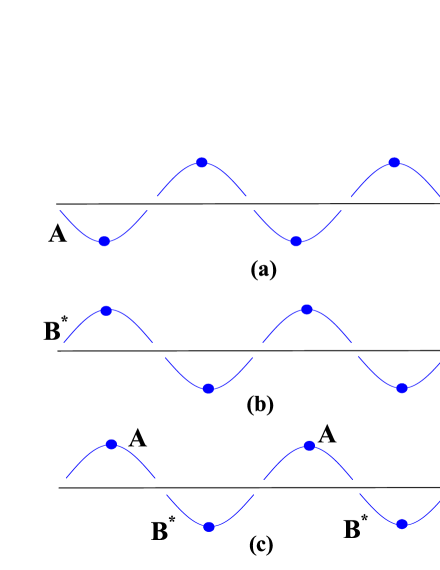
Figure 2: An illustration of knot states in vortex-representation: $\mathrm{A}$ and $\mathrm{B}$ denote two 1D vortex-lines. Here B^∗ denotes conjugate representation of vortex-line-B. The curves with blue dots denote knots on the knot-crystal – the curves with blue dot above the line are denoted by $c_{i}^{\dagger}\left|0\right\rangle$ and the curves with blue dot below the line are denoted by $(c_{i}^{\dagger}\left|0\right\rangle)^{\dagger}$.

In this paper, we derive the effective Dirac model for a knot-crystal based on a representation of vortex degrees of freedom. We call it vortex-representation.

In Ref.kou , it was known that a knot has four degrees of freedom, two spin degrees of freedom $\uparrow$ or $\downarrow$ from the helicity degrees of freedom, the other two vortex degrees of freedom from the vortex degrees of freedom that characterize the vortex-membranes, $\mathrm{A}$ or $\mathrm{B}$. The basis to define the microscopic structure of a knot is given by $\left|\uparrow,\mathrm{A}\right\rangle,$ $\left|\uparrow,\mathrm{B}\right\rangle,$ $\left|\downarrow,\mathrm{A}\right\rangle,$ $\left|\downarrow,\mathrm{B}\right\rangle.$

We define operator of knot states by the region of the phase angle of a knot: for the case of $\phi_{0}\operatorname{mod}(2\pi)\in(-\pi,0],$ we have $c^{\dagger}\left|0\right\rangle$; For the case of $\phi_{0}\operatorname{mod}(2\pi)\in(0,\pi],$ we have $(c^{\dagger}\left|0\right\rangle)^{\dagger}$. As shown in Fig.2, we label the knots by Wannier state $\left|i,\mathrm{A,\uparrow}\right\rangle,$ $\left|i+1,\mathrm{A,\uparrow}\right\rangle^{\ast},$ $\left|i+2,\mathrm{A,\uparrow}\right\rangle$, $\left|i+3,\mathrm{A,\uparrow}\right\rangle^{\ast}$…

To characterize the energy cost from global winding, we use an effective Hamiltonian to describe the coupling between 2-knot states along $x^{I}$-direction on 3D SOC knot-crystal

$$Jc_{\mathrm{A/B}i}^{\dagger}T_{\mathrm{A/B,A/B}}^{I}c_{\mathrm{A/B},i+e^{I}}$$ (25)

with the annihilation operator of knots at the site $i,$ $c_{\mathrm{A/B},i}=\left(\begin{array}[c]{c}c_{\mathrm{A/B,}\uparrow,i}\\ c_{\mathrm{A/B,}\downarrow,i}\end{array}\right)$. $J$ is the coupling constant between two nearest-neighbor knots. According to the generalized translation symmetry, the transfer matrices $T_{\mathrm{A/B,A/B}}^{I}$ along $x^{I}$-direction are defined by

$$T_{\mathrm{A,A}}^{I}=T_{\mathrm{B,B}}^{I}=e^{ia(\hat{k}^{I}\cdot\sigma^{I})}$$ (26)

and

$$T_{\mathrm{A,B}}^{I}=T_{\mathrm{B,A}}^{I}=0.$$ (27)

After considering the spin rotation symmetry and the symmetry of vortex-membrane-A and vortex-membrane-B, the effective Hamiltonian from global winding energy can be described by a familiar formulation

$$\mathcal{H}_{\mathrm{coupling}}=\mathcal{\hat{H}}_{\mathrm{coupling,B}}+\mathcal{\hat{H}}_{\mathrm{coupling,A}}$$ (28)

where

$$\mathcal{\hat{H}}_{\mathrm{coupling,A}}=J{\displaystyle\sum\limits_{i,I}}c_{\mathrm{A,}i}^{\dagger}e^{ia(\hat{k}^{I}\cdot\sigma^{I})}c_{\mathrm{A},i+e^{I}}+h.c.$$ (29)

and

$$\mathcal{\hat{H}}_{\mathrm{coupling,B}}=J{\displaystyle\sum\limits_{i,I}}c_{\mathrm{B,}i}^{\dagger}e^{ia(\hat{k}^{I}\cdot\sigma^{I})}c_{\mathrm{B},i+e^{I}}+h.c.$$ (30)

We then use path-integral formulation to characterize the effective Hamiltonian for a knot-crystal as

$$\int\mathcal{D}\psi^{\dagger}(t,\vec{x})\mathcal{D}\psi(t)e^{i\mathcal{S}/\hbar}$$ (31)

where $\mathcal{S}=\int\mathcal{L}dt$ and $\mathcal{L}=i{\displaystyle\sum\limits_{i}}\psi_{i}^{\dagger}\partial_{t}\psi_{i}-\mathcal{H}_{\mathrm{coupling}}$. To describe the knot states on 3D knot-crystal, we have introduced a four-component fermion field to be

$$\psi(\mathbf{x})=\left(\begin{array}[c]{c}\psi_{\mathrm{A,}\uparrow}(t,\vec{x})\\ \psi_{\mathrm{B,}\uparrow}(t,\vec{x})\\ \psi_{\mathrm{A,}\downarrow}(t,\vec{x})\\ \psi_{\mathrm{B,}\downarrow}(t,\vec{x})\end{array}\right)$$ (32)

where $\mathrm{A},\mathrm{B}$ label vortex degrees of freedom and $\uparrow,\downarrow$ label two spin degrees of freedom that denote the two possible winding directions along a given direction $\vec{e}$.

In continuum limit, we have

$$\mathcal{H}_{\mathrm{coupling}} =\mathcal{\hat{H}}_{\mathrm{coupling,B}}+\mathcal{\hat{H}}_{\mathrm{coupling,A}}$$

$$=2aJ{\displaystyle\sum\limits_{k}}\psi_{\mathrm{A,}k}^{\dagger}[\sigma_{x}\cos k_{x}+\sigma_{y}\cos k_{y}+\sigma_{z}\cos k_{z}]\psi_{\mathrm{A,}k}$$

$$+2aJ{\displaystyle\sum\limits_{k}}\psi_{\mathrm{B,}k}^{\dagger}[\sigma_{x}\cos k_{x}+\sigma_{y}\cos k_{y}+\sigma_{z}\cos k_{z}]\psi_{\mathrm{B,}k}$$ (33)

where the dispersion of knots is

$$E_{\mathrm{A/B,}k}\simeq c_{\mathrm{eff}}[(\vec{k}-\vec{k}_{0})\cdot\vec{\sigma}],$$ (34)

where $\vec{k}_{0}=(\frac{\pi}{2},\frac{\pi}{2},\frac{\pi}{2})$ and $c_{\mathrm{eff}}=2aJ$ is the velocity. In the following part we ignore $\vec{k}_{0}$.

Next, we consider the mass term from leapfrogging motion, of which the angular frequency $\omega^{\ast}$. For leapfrogging motion obtained by1 , the function of the two entangled vortex-membranes at a given point in geometric space is simplified by

$$\left(\begin{array}[c]{c}\mathrm{z}_{\mathrm{A}}(\vec{x}=0,t)\\ \mathrm{z}_{\mathrm{B}}(\vec{x}=0,t)\end{array}\right)=\frac{r_{0}}{2}\left(\begin{array}[c]{c}1+e^{i\omega^{\ast}t}\\ 1-e^{i\omega^{\ast}t}\end{array}\right).$$ (35)

At $t=0$, we have $\left(\begin{array}[c]{c}\mathrm{z}_{\mathrm{A}}(\vec{x},t)\\ \mathrm{z}_{\mathrm{B}}(\vec{x},t)\end{array}\right)=\left(\begin{array}[c]{c}1\\ 0\end{array}\right)$; At $t=\frac{\pi}{\omega^{\ast}}$, we have $\left(\begin{array}[c]{c}\mathrm{z}_{\mathrm{A}}(\vec{x},t)\\ \mathrm{z}_{\mathrm{B}}(\vec{x},t)\end{array}\right)=\left(\begin{array}[c]{c}0\\ 1\end{array}\right).$ The leapfrogging knot-crystal leads to periodic varied knot states, i.e. at $t=0$ we have a knot on vortex-membrane-A that is denoted by $\left|\sigma,\mathrm{A}\right\rangle;$ at $t=\frac{\pi}{\omega^{\ast}}$ we have a knot on vortex-membrane-B denoted by $\left|\sigma,\mathrm{B}\right\rangle$. As a result, the leapfrogging motion becomes a global winding along time direction, $\left|t,\mathrm{A}\right\rangle,$ $\left|t+\frac{\pi}{\omega^{\ast}},\mathrm{B}\right\rangle,$ $\left|t+\frac{2\pi}{\omega^{\ast}},\mathrm{A}\right\rangle$, $\left|t+\frac{3\pi}{\omega^{\ast}},\mathrm{B}\right\rangle,$ … See the illustration of vortex-representation of knot states for knot-crystal in Fig.2(c). After a time period $t=\frac{\pi}{\omega^{\ast}},$ a knot state $\phi_{\mathrm{A}}\operatorname{mod}(2\pi)\in(-\pi,0]$ turns into a knot state $\phi_{\mathrm{B}}\operatorname{mod}(2\pi)\in(-\pi,0].$ Thus, we use the following formulation to characterize the leapfrogging process,

$$\psi_{\mathrm{A}}^{\dagger}\psi_{\mathrm{B}}^{\dagger}.$$ (36)

After considering the energy from the leapfrogging process, a corresponding term is given by

$$2\hbar_{\mathrm{knot}}\omega^{\ast}\psi_{\mathrm{A}}^{\dagger}\psi_{\mathrm{B}}^{\dagger}+h.c.$$ (37)

From the global rotating motion denoted $e^{-i\omega_{0}t},$ the winding states also change periodically. Because the contribution from global rotating motion $e^{-i\omega_{0}t}$ is always canceled by shifting the chemical potential, we don’t consider its effect.

From above equation, in the limit $\left|\vec{k}\right|\rightarrow 0$ we derive low energy effective Hamiltonian as

$$\mathcal{H}_{\mathrm{3D}} \simeq 2aJ{\displaystyle\sum\limits_{k}}\psi_{\mathrm{A,}k}^{\dagger}(\vec{\sigma}\cdot\vec{k})\psi_{\mathrm{A,}k}$$

$$+2aJ{\displaystyle\sum\limits_{k}}\psi_{\mathrm{B,}k}^{\dagger}(\vec{\sigma}\cdot\vec{k})\psi_{\mathrm{B,}k}$$

$$+2\hbar_{\mathrm{knot}}\omega^{\ast}{\displaystyle\sum\nolimits_{k,\sigma}}\psi_{\mathrm{A,\sigma,}k}^{\dagger}\psi_{\mathrm{B,\sigma,}k}^{\dagger}$$ (38)

$$=c_{\mathrm{eff}}\int\Psi^{\dagger}[\tau_{z}\otimes(\vec{\sigma}\cdot\hat{k})]\Psi d^{3}x$$

$$+m_{\mathrm{knot}}c_{\mathrm{eff}}^{2}\int\Psi^{\dagger}(\tau_{x}\otimes\vec{1})\Psi d^{3}x.$$ (39)

where

$$\Psi(\mathbf{x})=\left(\begin{array}[c]{c}\psi_{\mathrm{A,}\uparrow}(t,\vec{x})\\ \psi_{\mathrm{B,}\uparrow}^{\ast}(t,\vec{x})\\ \psi_{\mathrm{A,}\downarrow}(t,\vec{x})\\ \psi_{\mathrm{B,}\downarrow}^{\ast}(t,\vec{x})\end{array}\right).$$ (40)

We then re-write the effective Hamiltonian to be

$$\mathcal{H}_{\mathrm{3D}}=\int(\Psi^{\dagger}\hat{H}_{\mathrm{3D}}\Psi)d^{3}x$$ (41)

and

$$\hat{H}_{\mathrm{3D}}=c_{\mathrm{eff}}\vec{\Gamma}\cdot\vec{p}_{\mathrm{knot}}+m_{\mathrm{knot}}c_{\mathrm{eff}}^{2}\Gamma^{5}$$ (42)

where

$$\Gamma^{5} =\tau^{x}\otimes\vec{1}\mathbf{,}\text{ }\Gamma^{1}=\tau^{z}\otimes\sigma^{x},$$ (43)

$$\Gamma^{2} =\tau^{z}\otimes\sigma^{y},\text{ }\Gamma^{3}=\tau^{z}\otimes\sigma^{z}.$$

$\vec{p}=\hbar_{\mathrm{knot}}\vec{k}$ is the momentum operator. $\Psi^{\dagger}=(\psi_{\mathrm{A},\uparrow}^{\ast},\psi_{\mathrm{B},\uparrow},\psi_{\mathrm{A},\downarrow}^{\ast},\psi_{\mathrm{B},\downarrow})$ is the annihilation operator of four-component fermions. $m_{\mathrm{knot}}c_{\mathrm{eff}}^{2}=2\hbar_{\mathrm{knot}}\omega^{\ast}$ plays role of the mass of knots and $c_{\mathrm{eff}}=\frac{2a\cdot J}{\hbar_{\mathrm{knot}}}$ play the role of light speed where $a$ is a fixed length that denotes the half pitch of the windings on the knot-crystal. In the following parts, we set $\hbar_{\mathrm{knot}}=1$ and $c_{\mathrm{eff}}=1$.

Due to Lorentz invariance (see below discussion), the geometric space becomes geometric space-time, i.e., $(x,y,z)\rightarrow(x,y,z,t)$. Here, we may consider $\vec{\Gamma}$ and $\Gamma^{5}$ to be entanglement matrices along spatial and tempo direction in winding space-time, respectively. A complete set of entanglement matrices $(\vec{\Gamma},$ $\Gamma^{5})$ is called entanglement pattern. The coordinate transformation along x/y/z/t-direction is characterize by $e^{i\vec{\Gamma}\cdot\hat{k}\cdot\vec{x}}$ and $e^{i\Gamma^{5}\cdot\hat{\omega}t}$, respectively. Now, the knot becomes topological defect of 3+1D entanglement – a knot is not only anti-phase changing along arbitrary spatial direction $\vec{e}$ but also becomes anti-phase changing along tempo direction (along tempo direction, a knot switches a knot state $\left|\mathrm{A/B}\right\rangle$ to another knot state $\left|\mathrm{B/A}\right\rangle$).

Finally, the low energy effective Lagrangian of 3D SOC knot-crystal is obtained as

$$\mathcal{L}_{\mathrm{3D}} =i\Psi^{\dagger}\partial_{t}\Psi-\mathcal{H}_{\mathrm{3D}}$$ (44)

$$=\bar{\Psi}(i\gamma^{\mu}\hat{\partial}_{\mu}-m_{\mathrm{knot}})\Psi$$

where $\bar{\Psi}=\Psi^{\dagger}\gamma^{0},$ $\gamma^{\mu}$ are the reduced Gamma matrices,

$$\gamma^{1}=\gamma^{0}\Gamma^{1},\text{ }\gamma^{2}=\gamma^{0}\Gamma^{2},\text{ }\gamma^{3}=\gamma^{0}\Gamma^{3},$$ (45)

and

$$\gamma^{0} =\Gamma^{5}=\tau_{x}\otimes\vec{1},$$ (46)

$$\gamma^{5} =i\gamma^{0}\gamma^{1}\gamma^{2}\gamma^{3}.$$

In addition, we point out that there exists intrinsic relationship between the knot states of sublattice-representation and the knot states of vortex-representation

$$\left(\begin{array}[c]{c}\left|\mathrm{A}\right\rangle\\ \left|\text{{B}}\right\rangle\end{array}\right)=\mathcal{U}\left(\begin{array}[c]{c}\left|\mathrm{L}\right\rangle\\ \left|\text{{R}}\right\rangle\end{array}\right)$$ (47)

where $\mathcal{U}=\exp[i\pi\left(\begin{array}[c]{cc}0&-i\\ i&0\end{array}\right)].$ From the sublattice-representation of knot states, the knot-crystal becomes an object with staggered R/L zeroes along x/y/z spatial directions and time direction; From the vortex-representation of knot states, the knot-crystal becomes an object with global winding along x/y/z spatial directions and time direction. See the illustration of knot states of vortex-representation on a knot-crystal in Fig.2.

III.1.3 Emergent Lorentz-invariance

We discuss the emergent Lorentz-invariance for knot states on a knot-crystal.

Since the Fermi-velocity $c_{\mathrm{eff}}$ only depends on the microscopic parameter $J$ and $a,$ we may regard $c_{\mathrm{eff}}$ to be ”light-velocity” and the invariance of light-velocity becomes an fundamental principle for the knot physics. The Lagrangian for massive Dirac fermions indicates emergent SO(3,1) Lorentz-invariance. The SO(3,1) Lorentz transformations $S_{\mathrm{Lor}}$ is defined by

$$S_{\mathrm{Lor}}\gamma^{\mu}S_{\mathrm{Lor}}^{-1}=\gamma^{\prime\mu}$$ (48)

($\mu=0,1,2,3$) and

$$S_{\mathrm{Lor}}\gamma^{5}S_{\mathrm{Lor}}^{-1}=\gamma^{5}.$$ (49)

For a knot state with a global velocity $\vec{v},$ due to SO(3,1) Lorentz-invariance, we can do Lorentz boosting on $(\vec{x},t)$ by considering the velocity of a knot,

$$t \rightarrow t^{\prime}=\frac{t-\vec{x}\cdot\vec{v}}{\sqrt{1-\vec{v}^{2}}},$$

$$\vec{x} \rightarrow\vec{x}^{\prime}=\frac{\vec{x}-\vec{v}\cdot t}{\sqrt{1-\vec{v}^{2}}}.$$ (50)

We can do non-uniform Lorentz transformation $S_{\mathrm{Lor}}(\vec{x},t)$ on knot states $\Psi(\vec{x},t).$ The inertial reference-frame for quantum states of the knot is defined under Lorentz boost, i.e.,

$$\Psi(\vec{x},t)\rightarrow\Psi^{\prime}(\vec{x}^{\prime},t^{\prime})=S_{\mathrm{Lor}}\cdot\Psi(\vec{x}^{\prime},t^{\prime}).$$ (51)

For a particle-like knot, a uniform wave-function of knot states $\psi(t)$ is

$$\psi(t)=\frac{1}{\sqrt{V}}e^{-i2\omega^{\ast}t}.$$ (52)

Under Lorentz transformation with small velocity $\left|\vec{v}\right|$, this wave-function $\psi(t)$ is transformed into

$$\psi(t) =\frac{1}{\sqrt{V}}e^{-i2\omega^{\ast}t}$$

$$\rightarrow\psi^{\prime}=\frac{1}{\sqrt{V}}e^{-i2\omega^{\ast}t^{\prime}}$$ (53)

$$\simeq\frac{1}{\sqrt{V}}e^{-i2\omega^{\ast}t}\exp(-i(E_{\mathrm{knot}}t-\vec{p}_{\mathrm{knot}}\cdot\vec{x}))$$

where $E_{\mathrm{knot}}\simeq\frac{\vec{p}_{\mathrm{knot}}^{2}}{2m_{\mathrm{knot}}},$ $\vec{p}_{\mathrm{knot}}\simeq\omega\vec{v}$ and $m_{\mathrm{knot}}c^{2}=2\omega^{\ast}.$ As a result, we derive a new distribution of knot-pieces by doing Lorentz transformation, that are described by the plane-wave wave-function $\frac{1}{\sqrt{V}}e^{-i2\omega^{\ast}t}\exp(-i(E_{\mathrm{knot}}t-\vec{p}_{\mathrm{knot}}\cdot\vec{x})).$ The new wave-function $\frac{1}{\sqrt{V}}\exp(-i(E_{\mathrm{knot}}t-\vec{p}_{\mathrm{knot}}\cdot\vec{x}))$ comes from the Lorentz boosting $S_{\mathrm{Lor}}$.

Noninertial system can be obtained by considering non-uniformly velocities, i.e., $\vec{v}\rightarrow\Delta\vec{v}(\vec{x},t).$ According to the linear dispersion for knots, we can do local Lorentz transformation on $(\vec{x},t)$ i.e.,

$$t \rightarrow t^{\prime}(\vec{x},t)=\frac{t-\vec{x}\cdot\Delta\vec{v}}{\sqrt{1-(\Delta\vec{v})^{2}}},$$ (54)

$$\vec{x} \rightarrow\vec{x}^{\prime}(\vec{x},t)=\frac{\vec{x}-\Delta\vec{v}\cdot t}{\sqrt{1-(\Delta\vec{v})^{2}}}.$$

We can also do non-uniform Lorentz transformation $S_{\mathrm{Lor}}(\vec{x},t)$ on knot states $\Psi(\vec{x},t),$ i.e.,

$$\Psi(\vec{x},t) \rightarrow\Psi^{\prime}(\vec{x}^{\prime}(\vec{x},t),t^{\prime}(\vec{x},t))$$ (55)

$$=S_{\mathrm{Lor}}(\vec{x},t)\cdot\Psi(\vec{x},t)$$

where the new wave-functions of all quantum states change following the non-uniform Lorentz transformation $S_{\mathrm{Lor}}(\vec{x},t)$. It is obvious that there exists intrinsic relationship between noninertial system and curved space-time.

III.2 Dirac model on winding space

In this part, we show the effective Dirac model of knot states on winding space.

The coordinate measurement of zero-lattice on winding space is the winding angles, $\vec{\Phi}$. Along a given direction $\vec{e}$, after shifting the distance $a,$ the windng angle changes $\pi.$ The position is determined by two kinds of values: $\vec{X}$ are integer numbers

$$\vec{X}=(X,Y,Z)=\frac{1}{\pi}\vec{\Phi}-\frac{1}{\pi}\vec{\Phi}\operatorname{mod}\pi$$ (56)

and $\vec{\phi}$ denote internal winding angles

$$\vec{\phi}=(\phi_{x},\phi_{y},\phi_{z})=\vec{\Phi}\operatorname{mod}\pi$$ (57)

with $\phi_{x},\phi_{y},\phi_{z}\in(0,\pi]$.

Therefore, on winding space, the effective Hamiltonian turns into

$$\hat{H}_{\mathrm{3D}} =\vec{\Gamma}\cdot\vec{p}_{\mathrm{knot}}+m_{\mathrm{knot}}\Gamma^{5}$$

$$=\vec{\Gamma}\cdot\vec{p}_{X,\mathrm{knot}}+\vec{\Gamma}\cdot\vec{p}_{\phi,\mathrm{knot}}+m_{\mathrm{knot}}\Gamma^{5}$$ (58)

where $\vec{p}_{X}=\frac{1}{a}i\frac{d}{d\vec{X}}$ and $\vec{p}_{\phi}=\frac{1}{a}i\frac{d}{d\vec{\phi}}$. Because of $\phi_{j}\in(0,\pi]$, quantum number of $\vec{p}_{\phi}$ is angular momentum $\vec{L}_{\phi}$ and the energy spectra are $\frac{1}{a}\left|\vec{L}_{\phi}\right|.$ If we focus on the low energy physics $E\ll\frac{1}{a}$ (or $\vec{L}_{\phi}=0$), we may get the low energy effective Hamiltonian as

$$\hat{H}_{\mathrm{3D}}\simeq\vec{\Gamma}\cdot\vec{p}_{X,\mathrm{knot}}+m_{\mathrm{knot}}\Gamma^{5}.$$ (59)

We introduce 3+1D winding space-time by defining four coordinates on winding space, $\Phi=(\vec{\Phi},\Phi_{t})$ where $\Phi_{t}$ is phase changing under time evolution. For a fixed entanglement pattern $(\vec{\Gamma},$ $\Gamma^{5})$, the coordinate transformation along x/y/z/t-direction on winding space-time is given by $e^{i\vec{\Gamma}\cdot\hat{\Phi}}$ and $e^{i\Gamma^{5}\cdot\hat{\Phi}_{t}}$, respectively.

For low energy physics, the position in 3+1D winding space-time is 3+1D zero-lattice of winding space-time labeled by four integer numbers, $\mathbf{X}=(\vec{X},X_{0})$ where

$$\vec{X} =\frac{1}{\pi}\vec{\Phi}-\frac{1}{\pi}\vec{\Phi}\operatorname{mod}\pi,\text{ }$$

$$X_{0} =\frac{1}{\pi}\Phi_{t}-\frac{1}{\pi}\Phi_{t}\operatorname{mod}\pi.$$ (60)

The lattice constant of the winding space-time is always $\pi$ that will never be changed. As a result, the winding space-time becomes an effective quantized space-time. Because of $x_{\mu}=a\cdot X_{\mu}$, the effective action on 3+1D winding space-time becomes

$$\mathcal{S}_{\mathrm{3D}}\simeq(a)^{4}\sum_{X,Y,Z,X_{0}}\mathcal{L}_{\mathrm{3D}}$$ (61)

where

$$\mathcal{L}_{\mathrm{3D}}=\bar{\Psi}[i\frac{1}{a}(\gamma^{\mu})\hat{\partial}_{\mu}-m_{\mathrm{knot}}]\Psi.$$ (62)

IV Deformed zero-lattice as curved space-time

In this section, we discuss the knot dynamics on smoothly deformed knot-crystal (or deformed zero-lattice). We point out that to characterize the entanglement evolution, the corresponding Biot-Savart mechanics for a knot on smoothly deformed zero-lattice is mapped to that in quantum mechanics on a curved space-time.

IV.1 Entanglement transformation

Firstly, based on a uniform 3D knot-crystal (uniform entangled vortex-membranes), we introduce the concept of ”entanglement transformation (ET)”.

Under global entanglement transformation, we have

$$\Psi(\vec{x},t)\rightarrow\Psi^{\prime}(\vec{x},t)=\hat{U}_{\mathrm{ET}}(\vec{x},t)\cdot\Psi(\vec{x},t)$$ (63)

where

$$\hat{U}_{\mathrm{ET}}(\vec{x},t)=e^{i\delta\vec{\Phi}\cdot\vec{\Gamma}}\cdot e^{i\delta\Phi_{t}\cdot\Gamma^{5}}.$$ (64)

Here, $\delta\vec{\Phi}$ and $\delta\Phi_{t}$ are constant winding angles along spatial $\vec{\Phi}$-direction and that along tempo direction on geometric space-time, respectively. The dispersion of the excitation changes under global entanglement transformation.

In general, we may define (local) entanglement transformation, i.e.,

$$\hat{U}_{\mathrm{ET}}(\vec{x},t)=e^{i\delta\vec{\Phi}(\vec{x}.t)\cdot\vec{\Gamma}}\cdot e^{i\delta\Phi_{t}(\vec{x}.t)\cdot\Gamma^{5}}$$ (65)

where $\delta\vec{\Phi}(\vec{x},t)$ and $\delta\Phi_{t}(\vec{x},t)$ are not constant. We call a system with smoothly varied-($\delta\vec{\Phi}(\vec{x},t)$, $\delta\Phi_{t}(\vec{x},t)$) deformed knot-crystal and its projected zero-lattice deformed (3+1D) zero-lattice.

IV.2 Geometric description for deformed zero-lattice – curved space-time

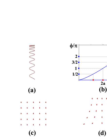
Figure 3: (a) An illustration of deformed knot-crystal; (b) An illustration of smoothly deformed relationship between winding angle $\Phi$ and spatial coordinate $x$. The zero-lattice in winding space is still uniform; while the zero-lattice in geometric space is deformed; (c) An illustration of a uniform 1+1D zero-lattice in geometric space-time; (d) An illustration of a deformed 1+1D zero-lattice in geometric space-time.

For knots on a deformed zero-lattice, there exists an intrinsic correspondence between an entanglement transformation $\hat{U}_{\mathrm{ET}}(\vec{x},t)$ and a local coordinate transformation that becomes a fundamental principle for emergent gravity theory in knot physics.

For zero-lattice, $\hat{U}_{\mathrm{ET}}(\vec{x},t)$ changes the winding degrees of freedom that is denoted by the local coordination transformation, i.e.,

$$\vec{\Phi}(\vec{x},t) \implies\vec{\Phi}^{\prime}(\vec{x},t)=\vec{\Phi}(\vec{x},t)+\delta\vec{\Phi}(\vec{x},t),$$

$$\Phi_{t}(\vec{x},t) \implies\Phi_{t}^{\prime}(\vec{x},t)=\Phi_{t}(\vec{x},t)+\delta\Phi_{t}(\vec{x},t).$$ (66)

These equations also imply a curved space-time: the lattice constants of the 3+1D zero-lattice (the size of a lattice constant with $2\pi$ angle changing) are not fixed to be $2a$, i.e.,

$$2a\rightarrow 2a_{\mathrm{eff}}(\vec{x},t)$$

The distance between two nearest-neighbor ”lattice sites” on the spatial/tempo coordinate changes, i.e.,

$$\Delta\vec{x} =(\vec{x}+\vec{e}_{x})-\vec{x}=\vec{e}_{x},$$ (67)

$$\Delta\vec{x}^{\prime} =(\vec{x}^{\prime}+\vec{e}_{x}^{\prime})-\vec{x}^{\prime}=\vec{e}_{x}^{\prime}(\vec{x},t)$$

and

$$\Delta t =(t+e_{0})-t=e_{0},$$ (68)

$$\Delta t^{\prime} =(t^{\prime}+e_{0}^{\prime})-t^{\prime}=e_{0}^{\prime}(\vec{x},t)$$

where $e_{a}$ $(a=0,1,2,3)$ and $e_{a}^{\prime}(\vec{x},t)$ are the unit-vectors of the original frame and the deformed frame, respectively. See the illustration of a 1+1D deformed zero-lattice on winding space-time with a non-uniform distribution of zeroes in Fig.3(d).

However, for deformed zero-lattice, the information of knots in projected space is invariant: when the lattice-distance of zero-lattice changes $a\rightarrow a_{\mathrm{eff}}(\vec{x},t)$, the size of the knots correspondingly changes $a\rightarrow a_{\mathrm{eff}}(\vec{x},t)$. Therefore, due to the invariance of a knot, the deformation of zero-lattice doesn’t change the formula of the low energy effective model for knots on winding space-time. Because one may smoothly deform the zero-lattice and get the same low energy effective model for knots on winding space-time, there exists diffeomorphism invariance, i.e.,

Knot-invariance on winding space-time

$$\implies\text{Diffeomorphism invariance.}$$ (69)

Therefore, from the view of mathematics, the physics on winding space-time is never changed! The invariance of the effective model for knots on winding space-time indicates the diffeomorphism invariance

$$\mathcal{S}_{\mathrm{zero-lattice}}\equiv(a)^{4}\sum_{X,Y,Z,X_{0}}\bar{\Psi}[i\frac{1}{a}\gamma^{\mu}\hat{\partial}_{\mu}^{X}-m_{\mathrm{knot}}]\Psi.$$ (70)

On the other hand, the condition of very smoothly entanglement transformation guarantees a (local) Lorentz invariance in long wave-length limit. Under local Lorentz invariance, the knot-pieces of a given knot are determined by local Lorentz transformations.

According to the local coordinate transformation, the deformed zero-lattice becomes a curved space-time for the knots. In continuum limit $\Delta k\ll(a)^{-1}$ and $\Delta\omega\ll\omega_{0}$, the diffeomorphism invariance and (local) Lorentz invariance emerge together. E. Witten had made a strong claim about emergent gravity, “whatever we do, we are not going to start with a conventional theory of non-gravitational fields in Minkowski space-time and generate Einstein gravity as an emergent phenomenon.” He pointed out that gravity could be emergent only if the notion on the space-time on which diffeomorphism invariance is simultaneously emergent. For the emergent quantum gravity in knot physics, diffeomorphism invariance and Lorentz invariance are simultaneously emergent. In particular, the diffeomorphism invariance comes from information invariance of knots on winding space-time – when the lattice-distance of zero-lattice changes, the size of the knots correspondingly changes.

To characterize the deformed 3+1D zero-lattice $\left(\vec{x}^{\prime}(\vec{x},t),t^{\prime}(\vec{x},t)\right)$, we introduce a geometric description. In addition to the existence of a set of vierbein fields $e^{a}$, the space metric is defined by $\eta_{ab}e_{\alpha}^{a}e_{\beta}^{b}=g_{\alpha\beta}$ where $\eta$ is the internal space metric tensor. The geometry fields (vierbein fields $e^{a}(\vec{x},t)$ and spin connections $\omega^{ab}(\vec{x},t)$) are determined by the non-uniform local coordinates $\left(\vec{x}^{\prime}(\vec{x},t),t^{\prime}(\vec{x},t)\right)$. Furthermore, one needs to introduce spin connections $\omega^{ab}(\vec{x},t)$ and the Riemann curvature 2-form as

$$R_{b}^{a} =d\omega_{b}^{a}+\omega_{c}^{a}\wedge\omega_{b}^{c}$$ (71)

$$=\frac{1}{2}R_{b\mu\nu}^{a}dx^{\mu}\wedge dx^{\nu},$$

where $R_{b\mu\nu}^{a}\equiv e_{\alpha}^{a}e_{b}^{\beta}R_{\beta\mu\nu}^{\alpha}$ are the components of the usual Riemann tensor projection on the tangent space. The deformation of the zero-lattice is characterized by

$$R^{ab}=d\omega^{ab}+\omega^{ac}\wedge\omega^{cb}.$$ (72)

So the low energy physics for knots on the deformed zero-lattice turns into that for Dirac fermions on curved space-time

$$\mathcal{S}_{\mathrm{curved-ST}}=\int\sqrt{-g}\bar{\Psi}(e_{a}^{\mu}\gamma^{a}(i\hat{\partial}_{\mu}+i\omega_{\mu})-m_{\mathrm{knot}})\Psi\text{ }d^{4}x$$ (73)

where $\omega_{\mu}=(\omega_{\mu}^{0i}\gamma^{0i}/2,\omega_{\mu}^{ij}\gamma^{ij}/2)$ ($i,j=1,2,3$) and $\gamma^{ab}=-\frac{1}{4}[\gamma^{a},\gamma^{b}]$ ($a,b=0,1,2,3$)23 . This model described by $\mathcal{S}_{\mathrm{curved-ST}}$ is invariant under local (non-compact) SO(3,1) Lorentz transformation $S(\vec{x},t)=e^{\theta_{ab}(\vec{x},t)\gamma^{ab}}$ as

$$\Psi(\vec{x},t) \rightarrow\Psi^{\prime}(\vec{x},t)=S(\vec{x},t)\Psi(\vec{x},t),$$

$$\gamma^{\mu} \rightarrow(\gamma^{\mu}(\vec{x},t))^{\prime}=S(\vec{x},t)\gamma^{\mu}(S(\vec{x},t))^{-1},$$

$$\omega_{\mu} \rightarrow\omega_{\mu}^{\prime}(\vec{x},t)=S(\vec{x},t)\omega_{\mu}(\vec{x},t)(S(\vec{x},t))^{-1}$$

$$+S(\vec{x},t)\partial_{\mu}(S(\vec{x},t))^{-1}.$$ (74)

$\gamma^{5}$ is invariant under local SO(3,1) Lorentz symmetry as

$$\gamma^{5} \rightarrow(\gamma^{5})^{\prime}=S(\vec{x},t)\gamma^{5}(S(\vec{x},t))^{-1}$$

$$=\gamma^{5}.$$ (75)

In general, an SO(3,1) Lorentz transformation $S(\vec{x},t)$ is a combination of spin rotation transfromation $\hat{R}(\vec{x},t)=\hat{R}_{\mathrm{spin}}(\vec{x},t)\cdot\hat{R}_{\mathrm{space}}(\vec{x},t)$ and Lorentz boosting $S_{\mathrm{Lor}}(\vec{x},t)$.

In physics, under a Lorentz transformation, a distribution of knot-pieces changes into another distribution of knot-pieces. For this reason, the velocity $c_{\mathrm{eff}}$ and the total number of zeroes $N_{\mathrm{knot}}$ are invariant,

$$c_{\mathrm{eff}}\rightarrow c_{\mathrm{eff}}^{\prime}\equiv c_{\mathrm{eff}}$$ (76)

and

$$N_{\mathrm{knot}}\rightarrow N_{\mathrm{knot}}^{\prime}\equiv N_{\mathrm{knot}}.$$ (77)

IV.3 Gauge description for deformed zero-lattice

IV.3.1 Deformed entanglement matrices and deformed entanglement pattern

The deformation of the zero-lattice leads to deformation of entanglement pattern, i.e.,

$$(\vec{\Gamma},\Gamma^{5})\rightarrow(\vec{\Gamma}^{\prime}(\mathbf{x}),(\Gamma^{5})^{\prime}(\mathbf{x}))$$ (78)

where

$$\vec{\Gamma}^{\prime}(\mathbf{x}) =\hat{U}_{\mathrm{ET}}(\mathbf{x})\vec{\Gamma}\hat{U}_{\mathrm{ET}}(\mathbf{x})^{-1},$$ (79)

$$(\Gamma^{5})^{\prime}(\mathbf{x}) =\hat{U}_{\mathrm{ET}}(\vec{x},t)\Gamma^{5}\hat{U}_{\mathrm{ET}}(\mathbf{x})^{-1}.$$

$\mathbf{x}$ denotes the space-time position of a site of zero-lattice, $(\vec{x},t)$. Each entanglement matrix becomes a unit SO(4) vector-field on each lattice site. The deformed zero-lattice induced by local entanglement transformation $\hat{U}_{\mathrm{ET}}(\mathbf{x})$ is characterized by four SO(4) vector-fields (four entanglement matrices) $(\vec{\Gamma}^{\prime}(\mathbf{x}),(\Gamma^{5})^{\prime}(\mathbf{x}))$. See the illustration of a 2D deformed zero-lattice in Fig.(4)d, in which the arrows denote deformed entanglement matrix $(\Gamma^{5})^{\prime}(\mathbf{x})$.

IV.3.2 Gauge description for deformed tempo entanglement matrix

Firstly, we stduy the unit SO(4) vector-field of deformed tempo entanglement matrix $(\Gamma^{5})^{\prime}(\mathbf{x}).$ To characterize $(\Gamma^{5})^{\prime}(\mathbf{x}),$ the reduced Gamma matrices $\gamma^{\mu}$ is defined as

$$\gamma^{1}=\gamma^{0}\Gamma^{1},\text{ }\gamma^{2}=\gamma^{0}\Gamma^{2},\text{ }\gamma^{3}=\gamma^{0}\Gamma^{3},$$ (80)

and

$$\gamma^{0} =\Gamma^{5}=\tau^{x}\otimes\vec{1},$$ (81)

$$\gamma^{5} =i\gamma^{0}\gamma^{1}\gamma^{2}\gamma^{3}.$$

Under this definition ($\gamma^{0}=\Gamma^{5}$), the effect of deformed zero-lattice from spatial entanglement transformation $e^{i\Gamma^{1}\cdot\Delta\Phi_{x}}$, $e^{i\Gamma^{2}\cdot\Delta\Phi_{y}}$, $e^{i\Gamma^{3}\cdot\Delta\Phi_{z}}$ can be studied due to

$$\Gamma^{5}\rightarrow(\Gamma^{5})^{\prime}(\mathbf{x})=\hat{U}_{\mathrm{ET}}^{x/y/z}(\vec{x},t)\Gamma^{5}\hat{U}_{\mathrm{ET}}^{x/y/z}(\mathbf{x})^{-1}\neq\Gamma^{5}.$$ (82)

However, the effect of deformed zero-lattice from tempo entanglement transformation $e^{i\delta\Phi_{t}\cdot\Gamma^{5}}$ cannot be well defined due to

$$\Gamma^{5}\rightarrow(\Gamma^{5})^{\prime}(\mathbf{x})=\hat{U}_{\mathrm{ET}}^{t}(\vec{x},t)\Gamma^{5}\hat{U}_{\mathrm{ET}}^{t}(\mathbf{x})^{-1}=\Gamma^{5}.$$ (83)

We introduce an SO(4) transformation $\hat{U}(\vec{x},t)$ that is a combination of spin rotation transfromation $\hat{R}(\mathbf{x})$ and spatial entanglement transformation (entanglement transformation along x/y/z-direction) $\hat{U}_{\mathrm{ET}}^{x/y/z}(\mathbf{x})=e^{i\delta\vec{\Phi}(\mathbf{x})\cdot\vec{\Gamma}}$, i.e.,

$$\hat{U}(\mathbf{x})=\hat{R}(\mathbf{x})\oplus\hat{U}_{\mathrm{ET}}^{x/y/z}(\mathbf{x}).$$ (84)

Here, $\oplus$ denotes operation combination. Under a non-uniform SO(4) transformation $\hat{U}(\mathbf{x})$, we have

$$\gamma^{0} \rightarrow\hat{U}(\mathbf{x})\gamma^{0}(\hat{U}(\mathbf{x}))^{-1}$$ (85)

$$=(\gamma^{0}(\mathbf{x}))^{\prime}={\displaystyle\sum\nolimits_{a}}\gamma^{a}n^{a}(\mathbf{x})$$

where $\mathbf{n}=(n^{1},n^{2},n^{3},\phi_{0}^{0})=(\vec{n},\phi_{0}^{0})$ is a unit SO(4) vector-field. For the deformed zero-lattice, according to $(\gamma^{0}(\mathbf{x}))^{\prime}\neq\gamma^{0},$ the entanglement matrix $\Gamma^{5}=\gamma^{0}$ along tempo direction is varied, $\Gamma^{5}\rightarrow(\Gamma^{5})^{\prime}(\mathbf{x})\neq\Gamma^{5}$.

In general, the SO(4) transformation is defined by $\hat{U}(\mathbf{x})=e^{\Phi_{ab}(\mathbf{x})\gamma^{ab}}$ ($\gamma^{ab}=-\frac{1}{4}[\gamma^{a},\gamma^{b}]$). Under the SO(4) transformation, we have

$$\gamma^{\mu} \rightarrow(\gamma^{\mu}(\mathbf{x)})^{\prime}=\hat{U}(\mathbf{x})\gamma^{\mu}(\hat{U}(\mathbf{x}))^{-1},$$

$$A_{\mu} \rightarrow A_{\mu}^{\prime}(\vec{x},t)=\hat{U}(\vec{x},t)A_{\mu}(\mathbf{x})(\hat{U}(\mathbf{x}))^{-1}$$

$$+\hat{U}(\mathbf{x})\partial_{\mu}(\hat{U}(\mathbf{x}))^{-1}.$$ (86)

In particular, $\gamma^{5}$ is invariant under the SO(4) transformation as

$$\gamma^{5} \rightarrow(\gamma^{5})^{\prime}=\hat{U}(\mathbf{x})\gamma^{5}(\hat{U}(\mathbf{x}))^{-1}$$

$$=\gamma^{5}.$$ (87)

The correspondence between index of $\gamma^{a}$ and index of space-time $x^{a}$ is

$$\gamma^{1} \Leftrightarrow x,\text{ }\gamma^{2}\Leftrightarrow y,$$ (88)

$$\gamma^{3} \Leftrightarrow z,\text{ }\gamma^{0}\Leftrightarrow t.$$

We denote this correspondence to be

$$(1,2,3,0)_{\mathrm{ET}}\Leftrightarrow(1,2,3,0)_{\mathrm{ST}}$$ (89)

where $(1,2,3,0)_{\mathrm{ET}}$ denotes the index order of $\gamma^{a}$ and $(1,2,3,0)_{\mathrm{ST}}$ denotes the index order of space-time $x^{a}$.

As a result, we can introduce an auxiliary gauge field $A_{\mu}^{ab}(\mathbf{x})$ and use a gauge description to characterize the deformation of the zero-lattice. The auxiliary gauge field $A_{\mu}^{ab}(\mathbf{x})$ is written into two parts23 : SO(3) parts

$$A^{ij}(\mathbf{x})=\mathrm{tr}(\gamma^{ij}(\hat{U}(\mathbf{x}))d(\hat{U}(\mathbf{x}))^{-1})$$ (90)

and SO(4)/SO(3) parts

$$A^{i0}(\mathbf{x}) =\mathrm{tr}(\gamma^{i0}\hat{U}(\mathbf{x}))d(\hat{U}(\mathbf{x}))^{-1})$$ (91)

$$=\gamma^{0}d(\gamma^{i}(\mathbf{x}))^{\prime}=-\gamma^{i}d\left(\gamma^{0}(\mathbf{x})\right)^{\prime}.$$

The total field strength $\mathcal{F}^{ij}(\mathbf{x})$ of $i,j=1,2,3$ components can be divided into two parts

$$\mathcal{F}^{ij}(\mathbf{x})=F^{ij}+A^{i0}\wedge A^{j0}.$$ (92)

According to pure gauge condition, we have Maurer-Cartan equation,

$$\mathcal{F}^{ij}(\mathbf{x})=F^{ij}+A^{i0}\wedge A^{j0}\equiv 0$$ (93)

or

$$F^{ij} =dA^{ij}+A^{ik}\wedge A^{kj}$$ (94)

$$\equiv-A^{i0}\wedge A^{j0}.$$

Finally, we emphasize the equivalence between $\gamma^{0i}$ and $\Gamma^{i}$, i.e., $\gamma^{0i}\Leftrightarrow\Gamma^{i}.$

IV.3.3 Gauge description for deformed spatial entanglement matrix

Next, we stduy the unit SO(4) vector-field of deformed spatial entanglement matrix $(\Gamma^{i})^{\prime}(\mathbf{x}).$ To characterize $(\Gamma^{i})^{\prime}(\mathbf{x}),$ the reduced Gamma matrices $\gamma^{\mu}$ is defined as

$$\gamma^{1}=\gamma^{0}\Gamma^{j},\text{ }\gamma^{2}=\gamma^{0}\Gamma^{k},\text{ }\gamma^{3}=\gamma^{0}\Gamma^{5},$$ (95)

and

$$\gamma^{0} =\Gamma^{i}=\tau^{z}\otimes\sigma^{i},$$ (96)

$$\gamma^{5} =i\gamma^{0}\gamma^{1}\gamma^{2}\gamma^{3}.$$

Here, $\Gamma^{i}$, $\Gamma^{j}$, and $\Gamma^{k}$ are three orthotropic spatial entanglement matrices. Under this definition ($\gamma^{0}=\Gamma^{i}$), the effect of deformed zero-lattice from partial spatial/tempo entanglement transformation $e^{i\Gamma^{j}\cdot\Delta\Phi_{j}}$, $e^{i\Gamma^{k}\cdot\Delta\Phi_{k}}$, $e^{i\Gamma^{5}\cdot\Delta\Phi_{t}}$ can be studied due to

$$\Gamma^{i}\rightarrow(\Gamma^{i})^{\prime}(\mathbf{x})=\hat{U}_{\mathrm{ET}}^{x_{j}/x_{k}/t}(\vec{x},t)\Gamma^{i}\hat{U}_{\mathrm{ET}}^{x_{j}/x_{k}/t}(\mathbf{x})^{-1}\neq\Gamma^{i}.$$ (97)

However, the effect of deformed zero-lattice from spatial entanglement transformation $e^{i\delta\Phi_{t}\cdot\Gamma^{5}}$ cannot be well defined due to

$$\Gamma^{i}\rightarrow(\Gamma^{i})^{\prime}(\mathbf{x})=\hat{U}_{\mathrm{ET}}^{x_{i}}(\vec{x},t)\Gamma^{i}\hat{U}_{\mathrm{ET}}^{x_{i}}(\mathbf{x})^{-1}=\Gamma^{i}.$$ (98)

We use similar approach to introduce the gauge description. We can also define the reduced Gamma matrices $\tilde{\gamma}^{\mu}$ as

$$\tilde{\gamma}^{1}=\tilde{\gamma}^{0}\Gamma^{2},\text{ }\tilde{\gamma}^{2}=\tilde{\gamma}^{0}\Gamma^{3},\text{ }\tilde{\gamma}^{3}=\tilde{\gamma}^{0}\Gamma^{5},$$ (99)

and

$$\tilde{\gamma}^{0} =\Gamma^{i}=\tau^{z}\otimes\sigma^{x},$$ (100)

$$\tilde{\gamma}^{5} =i\tilde{\gamma}^{0}\tilde{\gamma}^{1}\tilde{\gamma}^{2}\tilde{\gamma}^{3}.$$

The correspondence between index of $\tilde{\gamma}^{a}$ and index of space-time $x^{a}$ is

$$\tilde{\gamma}^{1} \Leftrightarrow y,\text{ }\tilde{\gamma}^{2}\Leftrightarrow z,$$ (101)

$$\tilde{\gamma}^{3} \Leftrightarrow t,\text{ }\tilde{\gamma}^{0}\Leftrightarrow x.$$

We denote this correspondence to be

$$(1,2,3,0)_{\mathrm{ET}}\Leftrightarrow(2,3,0,1)_{\mathrm{ST}}.$$ (102)

Now, the SO(4) transformation $\tilde{U}(\vec{x},t)=e^{\Phi_{ab}(\vec{x},t)\tilde{\gamma}^{ab}}$ ($\tilde{\gamma}^{ab}=-\frac{1}{4}[\tilde{\gamma}^{a},\tilde{\gamma}^{b}]$) is not a combination of spin rotation symmetry and entanglement transformation along x/y/z-direction. However, for the case of $a$ or $b$ to be $0,$ $\tilde{U}(\vec{x},t)=e^{\Phi_{a0}(\vec{x},t)\tilde{\gamma}^{a0}}$ denotes the entanglement transformation along y/z/t-direction. The unit SO(4) vector-field on each lattice site becomes

$$\tilde{U}(\mathbf{x})\tilde{\gamma}^{0}(\tilde{U}(\mathbf{x}))^{-1}=(\tilde{\gamma}^{0}(\mathbf{x}))^{\prime}={\displaystyle\sum\nolimits_{a}}\tilde{\gamma}^{a}\tilde{n}^{a}(\mathbf{x})$$ (103)

where $\mathbf{\tilde{n}}=(\tilde{n}^{1},\tilde{n}^{2},\tilde{n}^{3},\tilde{\phi}_{0}^{0})$ is a unit vector-field. The auxiliary gauge field $\tilde{A}^{ab}(\mathbf{x})$ are defined by

$$\tilde{A}^{ab}(\mathbf{x})=\mathrm{tr}(\tilde{\gamma}^{ij}(\tilde{U}(\mathbf{x}))d(\tilde{U}(\mathbf{x}))^{-1}).$$ (104)

According to pure gauge condition, we also have the following Maurer-Cartan equation,

$$\tilde{F}^{ij}=d\tilde{A}^{ij}+\tilde{A}^{ik}\wedge\tilde{A}^{kj}\equiv-\tilde{A}^{i0}\wedge\tilde{A}^{j0}.$$ (105)

Finally, we emphasize the equivalence between $\tilde{\gamma}^{0i}$ and $\Gamma^{a}$, i.e., $\tilde{\gamma}^{01}\Leftrightarrow\Gamma^{2},$ $\tilde{\gamma}^{02}\Leftrightarrow\Gamma^{3},$ $\tilde{\gamma}^{03}\Leftrightarrow\Gamma^{5}$.

IV.3.4 Hidden SO(4) invariant for gauge description

In addition, there exists a hidden global SO(4) invariant for entanglement matrices along different directions in 3+1D (winding) space-time $(\vec{\Gamma},\Gamma^{5})\rightarrow(\vec{\Gamma}^{\prime},(\Gamma^{5})^{\prime})$. To show the hidden SO(4) invariant, we define the reduced Gamma matrices $\tilde{\gamma}^{\mu}$ as

$$\tilde{\gamma}^{1} =\tilde{\gamma}^{0}\Gamma^{2},\text{ }\tilde{\gamma}^{2}=\tilde{\gamma}^{0}\Gamma^{3},\text{ }\tilde{\gamma}^{3}=\tilde{\gamma}^{0}\Gamma^{5},$$ (106)

$$\tilde{\gamma}^{0} =\alpha\Gamma^{1}+\beta\Gamma^{2}+\gamma\Gamma^{3}+\delta\Gamma^{5},$$

$$\tilde{\gamma}^{5} =i\tilde{\gamma}^{0}\tilde{\gamma}^{1}\tilde{\gamma}^{2}\tilde{\gamma}^{3}$$

with $\alpha^{2}+\beta^{2}+\gamma^{2}+\delta^{2}=1$. Here, $\alpha,$ $\beta,$ $\gamma,$ $\delta$ are constant.

Under this description, we can study the entanglement deformation along orthotropic spatial/tempo directions to $x^{\prime}=\alpha x+\beta y+\gamma z+\delta t$.

IV.4 Relationship between geometric description and gauge description for deformed zero-lattice

Due to the generalized spatial translation symmetry there exists an intrinsic relationship between gauge description for entanglement deformation between two vortex-membranes and geometric description for global coordinate transformation of the same deformed zero-lattice.

On the one hand, to characterize the changes of the positions of zeroes, we must consider a curved space-time by using geometric description, $\mathbf{x}=(\vec{x},t)\rightarrow\mathbf{x}^{\prime}=(\vec{x}^{\prime},t^{\prime})$. On the other hand, we need to consider a varied vector-field

$$(\gamma^{0}(\mathbf{x}))^{\prime} =\hat{U}(\mathbf{x})\gamma^{0}(\hat{U}(\mathbf{x}))^{-1}$$ (107)

$$={\displaystyle\sum\nolimits_{a}}\gamma^{a}n^{a}(\mathbf{x})$$

by using gauge description. There exists intrinsic relationship between the geometry fields $e^{a}(\mathbf{x})$ ($a=1,2,3,0$) and the auxiliary gauge fields $A^{a0}(\mathbf{x})$.

For a non-uniform zero-lattice, we have

$$\vec{\Phi}(\vec{x},t) \implies\vec{\Phi}^{\prime}(\vec{x},t)=\vec{\Phi}(\vec{x},t)+\delta\vec{\Phi}(\vec{x},t),$$

$$\Phi_{t}(\vec{x},t) \implies\Phi_{t}^{\prime}(\vec{x},t)=\Phi_{t}(\vec{x},t)+\delta\Phi_{t}(\vec{x},t).$$ (108)

On deformed zero-lattice, the ”lattice distances” become dynamic vector fields. We define the vierbein fields $e^{a}(\mathbf{x})$ that are supposed to transform homogeneously under the local symmetry, and to behave as ordinary vectors under local entanglement transformation along $x^{a}$-direction,

$$e^{a}(\mathbf{x})=dx^{a}(\mathbf{x})=\frac{a}{\pi}d\Phi^{a}(\mathbf{x}).$$ (109)

For the smoothly deformed vector-fields $n^{i}(\mathbf{x})\ll 1$, within the representation of $\Gamma^{5}=\gamma^{0}$ we have

$$\frac{d\Phi^{i}(\mathbf{x})}{2\pi} =n^{i}(\mathbf{x})=\mathrm{tr}[\gamma^{0}d\gamma^{i}(\mathbf{x})]$$

$$=A^{i0}(\mathbf{x}),\text{ }i=1,2,3.$$ (110)

Thus, the relationship between $e^{i}(\mathbf{x})$ and $A^{i0}(\mathbf{x})$ is obtained as

$$e^{i}(\mathbf{x})\equiv(2a)A^{i0}(\mathbf{x}).$$ (111)

According to this relationship, the changing of entanglement of the vortex-membranes curves the 3D space.

On the other hand, within the representation of $\Gamma^{i}=\tilde{\gamma}^{0}$ we have

$$\frac{d\Phi^{a}(\mathbf{x})}{2\pi} =\tilde{n}^{a}(\mathbf{x})=\mathrm{tr}[\tilde{\gamma}^{0}d\tilde{\gamma}^{a}(\mathbf{x})]$$

$$=\tilde{A}^{i0}(\mathbf{x}),\text{ }i=j,k,0,$$ (112)

and

$$e^{0}(\mathbf{x})=dt(\mathbf{x})=\frac{a}{\pi}d\Phi_{t}(\mathbf{x})=(2a)\tilde{A}^{30}(\mathbf{x}).$$ (113)

According to this relationship, the changing of entanglement of the vortex-membranes curves the 4D space-time.

In addition, we point out that for different representation of reduced Gamma matrix, there exists intrinsic relationships between the gauge fields $A(\mathbf{x})$ and $\tilde{A}(\mathbf{x}).$ After considering these relationships, we have a complete description of the deformed zero-lattice on the geometric space-time,

V Emergent gravity

Gravity is a natural phenomenon by which all objects attract one another including galaxies, stars, human-being and even elementary particles. Hundreds of years ago, Newton discovered the inverse-square law of universal gravitation, $F=\frac{GMm}{r^{2}}$ where $G$ is the Newton constant, $r$ is the distance, and $M$ and $m$ are the masses for two objects. One hundred years ago, the establishment of general relativity by Einstein is a milestone to learn the underlying physics of gravity that provides a unified description of gravity as a geometric property of space-time. From Einstein’s equations $R_{\mu\nu}-\frac{1}{2}Rg_{\mu\nu}=8\pi GT_{\mu\nu},$ the gravitational force is really an effect of curved space-time. Here $R_{\mu\nu}$ is the 2nd rank Ricci tensor, $R$ is the curvature scalar, $g_{\mu\nu}$ is the metric tensor, and $T_{\mu\nu}$ is the energy-momentum tensor of matter.

In this section, we point out that there exists emergent gravity for knots on zero-lattice.

V.1 Knots as topological defects

V.1.1 Knot as SO(4)/SO(3) topological defect in 3+1D space-time

A knot corresponds to an elementary object of a knot-crystal; A knot-crystal can be regarded as composite system of multi-knot. For example, for 1D knot, people divide the knot-crystal into $N$ identical pieces, each of which is just a knot.

From point view of information, each knot corresponds to a zero between two vortex-membranes along the given direction. For a knot, there must exist a zero point, at which $\xi_{\mathrm{A}}(x)$ is equal to $\xi_{\mathrm{B}}(x)$. The position of the zero is determined by a local solution of the zero-equation, $F_{\theta}(x)=0$ or $\xi_{\mathrm{A},\theta}(x)=\xi_{\mathrm{B},\theta}(x).$

From point view of geometry, a knot (an anti-knot) removes (or adds) a projected zero of zero-lattice that corresponds to removes (or adds) half of ”lattice unit” on the zero-lattice according to

$$\Delta x_{i}=\pm a_{\mathrm{eff}}(\vec{x},t)\simeq\pm a.$$ (114)

As a result, a knot looks like a special type of edge dislocation on 3+1D zero-lattice. The zero-lattice is deformed and becomes mismatch with an additional knot.

From point view of entanglement, a knot becomes topological defect of 3+1D winding spacet-time: along $x$-direction, knot is anti-phase changing denoted by $e^{i\Gamma^{1}\cdot\Delta\Phi_{x}}$, $\Delta\Phi_{x}=\pi;$ along $y$-direction, knot is anti-phase changing denoted by $e^{i\Gamma^{2}\cdot\Delta\Phi_{y}}$, $\Delta\Phi_{y}=\pi;$ along $z$-direction, knot is anti-phase changing denoted by $e^{i\Gamma^{3}\cdot\Delta\Phi_{z}}$, $\Delta\Phi_{z}=\pi;$ along $t$-direction, knot is anti-phase changing denoted by $e^{i\Gamma^{5}\cdot\Delta\Phi_{t}},$ $\Delta\Phi_{t}=\pi.$ Fig.4(a) and Fig.4(b) show an illustration a 1D knot.

In mathematics, to generate a knot at $(x_{0},y_{0},z_{0},t_{0})$, we do global topological operation on the knot-crystal, i.e.,

$$e^{i\Gamma^{1}\cdot\Delta\Phi_{x}(\mathbf{x})}\left|0\right\rangle$$ (115)

with $\Delta\Phi_{x}=0,$ $x<x_{0}$ and $\Delta\Phi_{x}=\pi,$ $x\geq x_{0};$

$$e^{i\Gamma^{2}\cdot\Delta\Phi_{y}(\mathbf{x})}\left|0\right\rangle$$ (116)

with $\Delta\Phi_{y}=0,$ $y<y_{0}$ and $\Delta\Phi_{y}=\pi,$ $y\geq y_{0};$

$$e^{i\Gamma^{3}\cdot\Delta\Phi_{z}(\mathbf{x})}\left|0\right\rangle$$ (117)

with $\Delta\Phi_{z}=0,$ $z<z_{0}$ and $\Delta\Phi_{z}=\pi,$ $z\geq x_{0};$

$$e^{i\Gamma^{5}\cdot\Delta\Phi_{t}(\mathbf{x})}\left|0\right\rangle$$ (118)

with $\Delta\Phi_{t}=0,$ $t<t_{0}$ and $\Delta\Phi_{t}=\pi,$ $t\geq t_{0}.$ As a result, due to the rotation symmetry in 3+1D space-time, a knot becomes SO(4)/SO(3) topologcal defect. Along arbitrary direction, the local entanglement matrices around a knot at center are switched on the tangentia sub-space-time.

V.1.2 Knot as SO(3)/SO(2) magnetic monopole in 3D space

To characterize the topological property of a knot on the 3+1D zero-lattice, we use gauge description. We firstly study the tempo entanglement deformation and define $\Gamma^{5}=\gamma_{0}.$ Under this gauge description, we can only study the effect of a knot on three spatial zero-lattice.

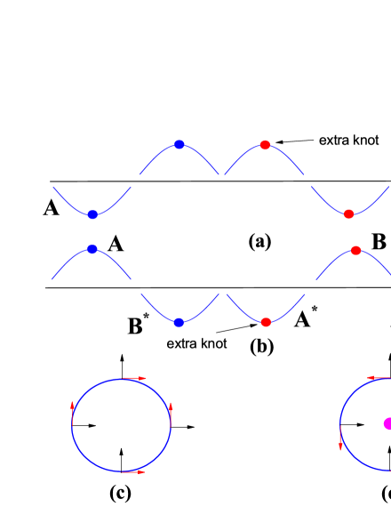
Figure 4: (a) An illustration of the effect of an extra knot on a 1D knot-crystal along spatial direction; (b) An illustration of the effect of an extra knot on a 1D knot-crystal along tempo direction. Here A^∗/B^∗ denotes conjugate representation of vortex-line-A/B; (c) The entanglement pattern for a uniform knot-crystal. The arrows denote the directions of entanglement matrices; (d) The entanglement pattern for a knot-crystal with an extra knot at center. The purple spot denotes the knot. The red arrows that denote local tangential entanglement matrices have vortex-like configuration on 2D projected space.

When there exists a knot, the periodic boundary condition of knot states along arbitrary direction is changed into anti-periodic boundary condition,

$$\Delta\Phi_{x}=\pi,\text{ }\Delta\Phi_{y}=\pi,\text{ }\Delta\Phi_{z}=\pi.$$ (119)

Consequently, along given direction (for example $x$-direction), the local entanglement matrices on the tangential sub-space are switched by $e^{i\Gamma^{1}\cdot\Delta\Phi_{x}}$ ($\Delta\Phi_{x}=\pi$). Along $x$-direction, in the limit of $x\rightarrow-\infty$, we have the local entanglement matrices on the tangential sub-space as $\Gamma^{2}$ and $\Gamma^{3}$; in the limit of $x\rightarrow\infty$, we have the local entanglement matrices on the tangential sub-space as $e^{i\Gamma^{1}\cdot\Delta\Phi_{x}}(\Gamma^{2})e^{-i\Gamma^{1}\cdot\Delta\Phi_{x}}=-\Gamma^{2}$ and $e^{i\Gamma^{1}\cdot\Delta\Phi_{x}}(\Gamma^{3})e^{-i\Gamma^{1}\cdot\Delta\Phi_{x}}=-\Gamma^{3}$.

Because we have similar result along $x^{i}$-direction for the system with an extra knot, the system has generalized spatial rotation symmetry. Due to the generalized spatial rotation symmetry, when moving around the knot, the local tangential entanglement matrices (we may use indices $j$, $k$ to denote the sub space) must rotate synchronously. See the red arrows that denote local tangential entanglement matrices in Fig.4(c) and Fig.4(d). In Fig.4(d), local tangential entanglement matrices induced by an extra (unified) knot shows vortex-like topological configuration in projected 2D space (for example, x-y plane). As a result, local tangential entanglement matrices induced by an extra knot can be exactly mapped onto that of an orientable sphere with fixed chirality.

To characterize the topological property of 3+1D zero-lattice with an extra (unified) knot, we apply gauge description and write down the following constraint

$${\displaystyle\iiint}\rho_{F}dV=\frac{1}{4\pi}{\displaystyle\iint}\epsilon_{jk}\epsilon_{ijk}F_{jk}^{jk}\cdot dS_{i}$$ (120)

where

$$F^{ij} =dA^{ij}+A^{ik}\wedge A^{kj}$$ (121)

$$\equiv-A^{i0}\wedge A^{j0}$$

and $\rho_{F}=\sqrt{-g}\psi^{\dagger}\psi.$ The upper indices of $F_{jk}^{jk}$ label the local entanglement matrices on the tangential sub-space and the lower indices of $F_{jk}^{jk}$ denote the spatial direction. The non-zero Gaussian integrate $\frac{1}{4\pi}{\displaystyle\iint}\epsilon_{jk}\epsilon_{ijk}F_{jk}^{jk}\cdot dS_{i}$ just indicates the local entanglement matrices on the tangential sub-space $A^{i0}\wedge A^{j0}$ to be the local frame of an orientable sphere with fixed chirality.

As a result, the entanglement pattern with an extra 3D knot is topologically deformed and the 3D knot becomes SO(3)/SO(2) magnetic monopole. From the point view of gauge description, a knot traps a ”magnetic charge” of the auxiliary gauge field, i.e.,

$$N_{F}=\int\sqrt{-g}\Psi^{\dagger}\Psi d^{3}x=q_{m}$$ (122)

where $q_{m}=\frac{1}{4\pi}{\displaystyle\iint}\epsilon_{jk}\epsilon_{ijk}F_{jk}^{jk}\cdot dS_{i}$ is the ”magnetic” charge of auxiliary gauge field $A^{jk}$. For single knot $N_{F}=1$, the ”magnetic” charge is $q_{m}=1$.

V.1.3 Knot as SO(3)/SO(2) magnetic monopole in 2+1D space-time

Next, we study the spatial entanglement deformation and define $\Gamma^{i}=\tilde{\gamma}_{0}.$ Under this gauge description, we can only study the effect of a knot on 2D spatial zero-lattice and 1D tempo zero-lattice.

In the 2+1D space-time, a knot also leads to $\pi$-phase changing,

$$\Delta\Phi_{i}=\pi,\text{ }\Delta\Phi_{j}=\pi,\text{ }\Delta\Phi_{t}=\pi.$$ (123)

Due to the spatial-tempo rotation symmetry, the knot also becomes SO(3)/SO(2) magnetic monopole and traps a ”magnetic charge” of the auxiliary gauge field $\tilde{A}^{jk}$, i.e.,

$$N_{F}=\int\sqrt{-g}\Psi^{\dagger}\Psi d^{3}x=\tilde{q}_{m}$$ (124)

where $\tilde{q}_{m}$ is the ”magnetic” charge of auxiliary gauge field $\tilde{A}^{ij}$. Remember that the correspondence between index of $\tilde{\gamma}^{i}$ and index of space-time $x^{i}$ is $\tilde{\gamma}^{1}\Leftrightarrow y,$ $\tilde{\gamma}^{2}\Leftrightarrow z,$ $\tilde{\gamma}^{3}\Leftrightarrow t.$

To characterize the induced magnetic charge, we write down another constraint

$${\displaystyle\iiint}\rho_{F}dV=\frac{1}{4\pi}{\displaystyle\iint}\epsilon_{ij}\epsilon_{ijk}\tilde{F}_{jk}^{ij}\cdot dS_{i}$$ (125)

where

$$\tilde{F}^{ij} =d\tilde{A}^{ij}+\tilde{A}^{ij}\wedge\tilde{A}^{ij}$$ (126)

$$\equiv-\tilde{A}^{i0}\wedge\tilde{A}^{j0}.$$

The upper indices of $\tilde{F}^{ij}=d\tilde{F}^{ij}+\tilde{F}^{ik}\wedge\tilde{F}^{kj}$ denote the local entanglement matrices on the tangential sub-space-time and the lower indices of $\tilde{F}_{jk}^{ij}$ denote the spatial direction. Therefore, according to above equation, the 2+1D zero-lattice is globally deformed by an extra knot.

In general, due to the hidden SO(4) invariant, for other gauge descriptions $\tilde{\gamma}^{0}=\alpha\Gamma^{1}+\beta\Gamma^{2}+\gamma\Gamma^{3}+\delta\Gamma^{5}$, a knot also play the role of SO(3)/SO(2) magnetic monopole and traps a ”magnetic charge” of the corresponding auxiliary gauge field.

V.2 Einstein-Hilbert action as topological mutual BF term for knots

It is known that for a given gauge description, a knot is an SO(3)/SO(2) magnetic monopole and traps a ”magnetic charge” of the corresponding auxiliary gauge field. For a complete basis of entanglement pattern, we must use four orthotropic SO(4) rotors $((\Gamma^{1})^{\prime}(\mathbf{x}),(\Gamma^{2})^{\prime}(\mathbf{x}),(\Gamma^{3})^{\prime}(\mathbf{x}),(\Gamma^{5})^{\prime}(\mathbf{x}))$ and four different gauge descriptions to characterize the deformation of a knot (an SO(4)/SO(3) topological defect) on a 3+1D zero-lattice.

Firstly, we use Lagrangian approach to characterize the deformation of a knot (an SO(3)/SO(2) topological defect) on a 3D spatial zero-lattice, $N_{F}=q_{m}$. The topological constraint in Eq.(120) can be re-written into

$$\frac{i}{4}\text{{tr}}\sqrt{-g}\bar{\Psi}\gamma^{i}(\gamma^{0i}/2)\Psi=\epsilon_{jk}\epsilon_{ijk}\frac{1}{4\pi}\hat{D}_{i}F_{jk}^{jk}$$ (127)

or

$$\frac{i}{4}\text{{tr}}\sqrt{-g}\bar{\Psi}\varpi_{0}^{0i}\gamma^{i}(\gamma^{0i}/2)\Psi=i\epsilon_{0ijk}\epsilon_{0ijk}\varpi_{0}^{0i}\frac{1}{4\pi}\hat{D}_{i}F_{jk}^{jk}$$ (128)

where $\hat{D}_{i}=i\hat{\partial}_{i}+i\omega_{i}$ is covariant derivative in 3+1D space-time. $\varpi^{0i}$ is a field that plays the role of Lagrangian multiplier. The upper index $i$ of $\varpi^{0i}$ denotes the local radial entanglement matrix around a knot, along which the entanglement matrix doesn’t change. Thus, we use the dual field $\varpi^{0i}$ to enforce the topological constraint in Eq.(120). That is, to denote the upper index of $F^{jk}$ that is the local tangential entanglement matrices, we set antisymmetric property of upper index of $\varpi^{0i}$ and that of $F^{jk}$. Because $\varpi^{0i}$ and $\omega^{0i}$ have the same SO(3,1) generator $(\gamma^{0i}/2)$, due to SO(3,1) Lorentz invariance we can do Lorentz transformation and absorb the dual field $\varpi^{0i}$ into $\omega^{0i}$, i.e., $\omega^{0i}\rightarrow(\omega^{0i})^{\prime}=\omega^{0i}+\varpi^{0i}$. As a result, the dual field $\varpi^{0i}$ is replaced by $\omega^{0i}$.

In the path-integral formulation, to enforce such topological constraint, we may add a topological mutual BF term $S_{\mathrm{MBF}}$ in the action that is

$$S_{\mathrm{MBF1}} =-\frac{1}{4\pi}\int\epsilon_{0ijk}\,\epsilon_{0\nu\lambda\kappa}\,R_{0\nu}^{0i}F_{\lambda\kappa}^{jk}\text{ }d^{4}x$$ (129)

$$=-\frac{1}{4\pi}\int\epsilon_{0ijk}\,R^{0i}\wedge F^{jk}$$

where

$$R^{0i}=d\omega^{0i}+\omega^{0j}\wedge\omega^{ji}.$$ (130)

From $F^{jk}\equiv-A^{j0}\wedge A^{k0}$ and $e^{i}\wedge e^{j}=(2a)^{2}A^{j0}\wedge A^{k0}.$ The induced topological mutual BF term $S_{\mathrm{MBF1}}$ is linear in the conventional strength in $R^{0i}$ and $F^{jk}$. This term is becomes

$$S_{\mathrm{MBF1}}=\frac{1}{4\pi(2a)^{2}}\int\epsilon_{0ijk}R^{0i}\wedge e^{j}\wedge e^{k}.$$ (131)

Next, we use Lagrangian approach to characterize the deformation of a knot (an SO(3)/SO(2) topological defect) on 2+1D space-time, $N_{F}=\tilde{q}_{m}$. Using the similar approach, we derive another topological mutual BF term $S_{\mathrm{MBF2}}$ in the action that is

$$S_{\mathrm{MBF2}} =-\frac{1}{4\pi}\int\epsilon_{0ijk}\,\epsilon_{0\nu\lambda\kappa}\,\tilde{R}_{0\nu}^{0i}\tilde{F}_{\lambda\kappa}^{jk}\text{ }d^{4}x$$ (132)

$$=-\frac{1}{4\pi}\int\epsilon_{0ijk}\,\tilde{R}^{0i}\wedge\tilde{F}^{jk}$$

where $\tilde{R}^{0i}=d\tilde{\omega}^{0i}+\tilde{\omega}^{0j}\wedge\tilde{\omega}^{ji}$. From $\tilde{F}^{k0}\equiv-\tilde{A}^{kj}\wedge\tilde{A}^{j0}$ and $\tilde{e}^{i}\wedge\tilde{e}^{j}=(2a)^{2}\tilde{A}^{j0}\wedge\tilde{A}^{k0},$ this term becomes

$$S_{\mathrm{MBF2}}=\frac{1}{4\pi(2a)^{2}}\int\epsilon_{ijk0}\tilde{R}^{0i}\wedge\tilde{e}^{j}\wedge\tilde{e}^{k}.$$ (133)

The upper index of $\tilde{R}^{0i}$ denotes entanglement transformation along given direction in winding space-time. We unify the index order of space-time into $(1,2,3,0)_{\mathrm{ST}}$ and reorganize the upper index. The topological mutual BF term becomes $\frac{1}{4\pi(2a)^{2}}\int\epsilon_{ijk0}R^{ij}\wedge e^{k}\wedge e^{0}.$ In Ref.mm ; mm1 ; mm2 ; mm4 , a topological description of Einstein-Hilbert action is proposed by S. W. MacDowell and F. Mansouri. The topological mutual BF term proposed in this paper is quite different from the MacDowell-Mansouri action.

According to the diffeomorphism invariance of winding space-time, there exists symmetry between the entanglement transformation along different directions. Therefore, with the help of a complete set of definition of reduced Gamma matrices $\gamma^{\mu},$ there exist other topological mutual BF terms $S_{\mathrm{MBF},i}.$ For the total topological mutual BF term $S_{\mathrm{MBF}}={\displaystyle\sum\limits_{i}}S_{\mathrm{MBF},i}$ that characterizes the deformation of a knot (an SO(4)/SO(3) topological defect) on a 3+1D zero-lattice, the upper index of the topological mutual BF term $R^{ij}\wedge e^{k}\wedge e^{l}$ must be symmetric, i.e., $i,j,k,l=1,2,3,0$.

By considering the SO(3,1) Lorentz invariance, the topological mutual BF term $S_{\mathrm{MBF}}$ turns into the Einstein-Hilbert action $S_{\mathrm{EH}}$ as

$$S_{\mathrm{MBF}} =S_{\mathrm{EH}}=\frac{1}{16\pi(a)^{2}}\int\epsilon_{ijkl}R^{ij}\wedge e^{k}\wedge e^{l}$$ (134)

$$=\frac{1}{16\pi G}\int\sqrt{-g}Rd^{4}x$$

where $G$ is the induced Newton constant which is $G=a^{2}.$ The role of the Planck length is played by $l_{p}=a$, that is the ”lattice” constant on the 3+1D zero-lattice.

Finally, from above discussion, we derived an effective theory of knots on deformed zero-lattice in continuum limit as

$$S =\mathcal{S}_{\mathrm{zero-lattice}}+S_{\mathrm{EH}}$$ (135)

$$=\int\sqrt{-g(x)}\bar{\Psi}(e_{a}^{\mu}\gamma^{a}\hat{D}_{\mu}-m_{\mathrm{knot}})\Psi\text{ }d^{4}x$$

$$+\frac{1}{16\pi G}\int\sqrt{-g}R\text{ }d^{4}x$$

where $\hat{D}_{\mu}=i\hat{\partial}_{\mu}+i\omega_{\mu}$. The variation of the action $S$ via the metric $\delta g_{\mu\nu}$ gives the Einstein’s equations

$$R_{\mu\nu}-\frac{1}{2}Rg_{\mu\nu}=8\pi GT_{\mu\nu}.$$ (136)

As a result, in continuum limit a knot-crystal becomes a space-time background like smooth manifold with emergent Lorentz invariance, of which the effective gravity theory turns into topological field theory.

For emergent gravity in knot physics, an important property is topological interplay between zero-lattice and knots. From the Einstein-Hilbert action, we found that the key property is duality between Riemann curvature $R^{ij}$ and strength of auxiliary gauge field $F^{kl}$: the deformation of entanglement pattern leads to the deformation of space-time.

In addition, there exist a natural energy cutoff $\hbar\omega_{0}$ and a natural length cutoff $a$. In high energy limit ($\Delta\omega\sim\omega_{0}$) or in short range limit ($\Delta x\sim a$), without well-defined 3+1D zero-lattice, there doesn’t exist emergent gravity at all.

VI Discussion and conclusion

In this paper, we pointed out that owing to the existence of local Lorentz invariance and diffeomorphism invariance there exists emergent gravity for knots on 3+1D zero-lattice. In knot physics, the emergent gravity theory is really a topological theory of entanglement deformation. For emergent gravity theory in knot physics, a topological interplay between 3+1D zero-lattice and the knots appears: on the one hand, the deformation of the 3+1D zero-lattice leads to the changes of knot-motions that can be denoted by curved space-time; on the other hand, the knots trapping topological defects deform the 3+1D zero-lattice that indicates matter may curve space-time. The Einstein-Hilbert action $S_{\mathrm{EH}}$ becomes a topological mutual BF term $S_{\mathrm{MBF}}$ that exactly reproduces the low energy physics of the general relativity. In table.1, we emphasize the relationship between modern physics and knot physics.

Modern physics	Knot Physics
Matter	Knot: a topological defect of 3+1 D zero-lattice
Motion	Changing of the distribution of knot-pieces
Mass	Angular frequency for leapfrogging motion
Inertial reference system	A knot under Lorentz boosting
Coordinate translation	Entanglement transformation
Space-time	3+1D zero-lattice of projected entangled vortex-membranes
Curved space-time	Deformed 3+1D zero-lattice
Gravity	Topological interplay between 3+1D zero-lattice and knots

Table 1: The relationship between modern physics and knot physics

In addition, this work would help researchers to understand the mystery in gravity. In modern physics, matter and space-time are two different fundamental objects and matter may move in (flat or curved) space-time. In knot physics, the most important physics idea for gravity is the unification of matter and space-time, i.e.,

$$\text{Matter (knots)}\iff\text{Space-time (zero-lattice).}$$ (137)

One can see that matter (knots) and space-time (zero-lattice) together with motion of matter are unified into a simple phenomenon – entangled vortex-membranes and matter (knots) curves space-time (3+1D zero-lattice) via a topological way.

- (1) W. Thomson, Phil. Mag. 10, 155 (1880).
- (2) R.J. Donnelly, Quantized Vortices in Helium II (Cambridge University Press, Cambridge 1991).
- (3) B. V. Svistunov, Phys. Rev. B52, 3647 (1995).
- (4) W. F. Vinen, Phys. Rev. B61, 1410 (2000).
- (5) F. W. Dyson, Part II Phil. Trans. R. Soc. Lond. A 184, 1041 (1893).
- (6) W. M. Hicks, Proc. R. Soc. Lond. A 102, 111 (1922).
- (7) A. V. Borisov, A. A. Kilin and I. S. Mamaev, Regul. Chaotic Dyn. 18, 33 (2013).
- (8) D. H. Wacks, A. W. Baggaley and C. F. Barenghi, Phys. Fluids 26, 027102 (2014).
- (9) R. M. Caplan, J. D. Talley, R. Carretero-González and P. G. Kevrekidis, Phys. Fluids 26, 097101 (2014).
- (10) N. Hietala, R. Hänninen, H. Salman, C. F. Barenghi, arXiv:1603.06403.
- (11) D. Kleckner, and W. T. M. Irvine, Nat. Phys. 9, 253(2013).
- (12) D. S. Hall, M. W. Ray, K. Tiurev, E. Ruokokoski, A. H. Gheorghe, and M. Möttönen, Nat. Phys. 12, 478(2016).
- (13) S. P. Kou, Int. J Mod. Phys. B 31, 1750241 (2017).
- (14) In this paper, we use , and,
- (15) S. W. MacDowell and F. Mansouri, Phys. Rev. Lett. 38, 739 (1977).
- (16) F. Mansouri, Phys. Rev. D 16 (1977) 2456.
- (17) P. Van Nieuwenhuizen, Phys. Rep. 68, 189 (1981).
- (18) A. Chamseddine and P. West, Nuc. Phys. B 129, 39 (1977).