Data Analysis of Massive Gravitational Waves from Gamma Ray Bursts

Abstract

We investigate the detectability of massive mode of polarization of Gravitational Waves (GWs) in $f(R)$ theory of gravity associated with Gamma Ray Bursts (GRBs) sources. We obtain the beam pattern function of Laser Interferometric Gravitational wave Observatory (LIGO) corresponding to the massive polarization of GWs and perform Bayesian analysis to study this polarization. It is found that the massive polarization component with a mass of $10^{-22}eV/c^{2}$ is too weak to be detected at LIGO with its current configuration.

PACS numbers:4.80.Nn, 95.55.Ym 04.30-w

1 Introduction

General Theory of Relativity (GTR) put forward by Einstein helps us to look at the Universe as a dynamic system amenable to mathematical formulations leading to have a standard cosmological model of the Universe. But there are problems with the standard cosmology based on GTR, both at the conceptual and at the cosmological/astrophysical levels[1]. The latest one being the observation that the Universe is now in an accelerating phase. During all these years, attempts are being made to modify or extend Einstein’s theory to find explanations for the drawbacks of GTR. Most of the recent studies are all cosmological, associated with or replacing the constructs like ‘inflation’ , ‘dark matter’  and ‘dark energy’. All these studies fall under the terminology ‘Extended Theories of Gravity (ETG)’  or ‘Alternative Theories of Gravity’ [2]. As a road to achieving modifications of GTR for getting a correct explanation for the current astronomical observations, it is better to consider a toy model as a tool to explain the limitations of GTR and to test whether the resulting ETG form the right path to modifying GTR. $f(R)$ theories of gravity[2] form the simplest class of extended or modified theories of gravity. Recently, massive gravity[3, 4] is receiving great attention, as this model can be used to explain dark energy problem associated with the late accelerating expansion of the Universe.

$f(R)$ theory comes out as a straight forward generalization of Einstein-Hilbert action for gravity and is given by,

$$S=\frac{1}{2\kappa}{\displaystyle\int}d^{4}x\sqrt{-g}f(R),$$ (1)

where $\kappa=8\pi G,$ $G$ is the gravitational constant ($c=1$), $g$ is the determinant of the metric tensor, $R$ is the Ricci scalar and $f(R)$ is the generalization of $R$. $f(R)$ theory of gravity makes a good toy model for two reasons[2]: $a)$ they are sufficiently general to encapsulate some of the basic characteristics of theories of gravity involving higher-order curvature invariants, but at the same time they are simple enough to be easy to handle and $b)$ they are unique among theories of gravity involving higher-order curvature invariants, in the sense that they seem to be the only ones which can avoid the long known and fatal Ostrogradski instability[5].

The existence of Gravitational Waves (GWs) is a natural outcome of GTR[6]. With the path breaking discovery of GWs, supposed to be from binary black hole merger[7], Laser Interferometer Gravitational Wave Observatory (LIGO) serves as the center of attention for future research in Gravitational Wave astronomy. A second detection of GWs from the coalescence of two-stellar mass black holes is also reported[8]. LIGO has got three specialized Michelson interferometers located at two sites $a)$ Hanford, $4$km-long H1 and $2$km long H$2$ detector $b)$ at Livingston, a $4$km long L$1$ detector[9]. Of the different GW sources present, one of the most important classes that still lacks a complete explanation is the Gamma Ray Bursts (GRBs). Studies are going on and new developments are being made in understanding this phenomenon. GRBs are intense flashes of $\gamma$-rays which occur approximately once per day and are isotropically distributed over the sky[10, 11]. Currently favored models of GRB progenitors are grouped into two broad classes by their characteristic duration and spectral hardness: $a)$ short GRB, the progenitors of which are thought to be mergers of neutron star binaries or neutron-star black hole binaries[12, 13] and $b)$ long GRB which are associated with core-collapse supernovae[14]. Both mergers and supernovae scenarios result in the formation of stellar-mass black holes with accretion disk and the emission of GWs are expected in this process. For the reasons mentioned above, GRBs form good sources of gravitational radiation[15, 16].

Strong-field regimes form the best testing ground for the ETG and GRBs provide a good strong-field regime for understanding alternative theories of gravity. In the recent studies on the discovery of GWs[17], it is to be noted that no studies were done aiming at constraining parameters corresponding to any of the alternative theories of gravity due to lack of predictions for what the inspiral-merger-ringdown GW signal would look like in those cases and no investigations were done for measuring the non-transverse[18] components of GWs. All the facts throw motivation for the modelling and parameter estimation of a GW event occurring from GRB that is described by ETG. Testing of GWs in alternative theories of gravity are discussed in general in the literature[18, 19, 20, 21, 22]. However, it is to be noted that the production and detection of GWs on the basis of ETG for GRB sources are not explored much.

The detection of GWs involves the statistical analysis of the observed data. It should tell whether the data contain the signal or not or whether the data supports a certain theoretical model or not with reliability. Statistical analysis can follow one of the two perspectives: 1) Frequentist/Classical analysis 2) Bayesian analysis. In a frequentist analysis, the probabilities are viewed in terms of the frequencies of random repeatable events whereas probabilities in Bayesian analysis provide a quantification of uncertainty[23]. From a Bayesian perspective, we can use the machinery of probability theory to describe the uncertainty in model parameters or in the choice of the model itself[24]. Bayesian analysis can be parametric or non parametric. Non parametric models constitute an approach to model selection and adaptation where sizes of models are allowed to grow with data size whereas in parametric models, a fixed number of parameters are used[25]. A Bayesian formulation of non parametric problem is non trivial since a Bayesian model defines the prior and posterior distribution on a single fixed parameter space, but the dimension of this parameter space in a non parametric approach changes with the sample size[26].

So, inspired by the recent observation of GWs, in this paper we make an attempt to study massive GWs from $f(R)$ theory of gravity, a class of ETG. Also we study the possibilities of detecting massive polarization component of GWs emanating from GRBs from such a theory at LIGO. The paper is organized as follows: In Section $2$, the antenna response functions for the $f(R)$ theory of gravity are found out and the beam pattern is figured for seven random GRB candidates. A Bayesian non parametric approach towards the signal detection of the massive polarization from GRB is studied in Section $3$. In Section $4$ massive GW signal from simulated data is analyzed with the help of Bayes factor and the probable Signal to Noise Ratio is calculated. Section $5$ concludes the paper.

2 Response function of LIGO detectors towards massive gravitational waves

The vacuum field equation of metric $f(R)$ gravity from $(1)$ is given by,

$$f^{\prime}(R)R_{\mu\nu}-\frac{1}{2}f(R)g_{\mu\nu}-(\nabla_{\mu}\nabla_{\nu}-g_{\mu\nu}\square)f^{\prime}(R)=0.$$ (2)

Taking $f(R)$ to be of the specific form, $f(R)=R+\lambda R^{2}$, where $\lambda$ is a constant, the general solutions of this equation are,

$$\bar{h}_{\mu\nu}={\displaystyle\int}A(k)\exp(-i(k.r-\omega t))dk,$$ (3)

and,

$$\bar{h}_{\mu\nu}={\displaystyle\int}A(k)\exp(-i(k.r-\omega_{m}t))dk,$$ (4)

where $\omega\neq\omega_{m}$[27, 28, 29].

In GTR there are only two polarizations for gravitational radiation, $+$ and $\times$. A scalar component of gravitational radiation in Brans-Dicke theory has been proposed and the detection of such a component has also been discussed in Ref. $[30]$. Recently it is shown in Ref. $[31]$ that semi-classical effective field theory also admits massless scalar GW solution in addition to conventional polarization modes of GTR. The paper also discusses astrophysical sources of scalar GWs. The utilization of metric $f(R)$ gravity results in additional polarization sates compared to the usual polarization states, $+$ and $\times$ in GTR.

In $f(R)$ theory, GWs can have a massive scalar mode besides the usual transverse-traceless modes in GTR. Six polarization modes are possible in $f(R)$ theories[32]. A recent study[33] shows that in metric $f(R)$ theory in addition to the $+$ and $\times$, a breathing mode which goes along with the $+$ and $\times$ modes and a longitudinal scalar mode which moves propagating along the direction of propagation of the GWs with a velocity less than the velocity of light exist. But in Palatini formalism $f(R)$ theories possess only the usual transverse-traceless modes as in GTR. GWs in most of the extended theories of gravity possess more than the two usual polarization modes. The detection of GWs is particularly a challenging issue and it may be capable of distinguishing the different modes and may help us to find the correct formulation of gravity. In this paper, we consider, only the case of massive scalar polarization component[34].

The effect of GWs is to produce a transverse shear strain and this fact makes the Michelson interferometer an obvious candidate for a detector. When GWs pass through the detector, then one arm of the detector gets stretched in one direction whereas the other arm gets compressed. The dimensionless detector response function $h$ of an interferometric detector is defined as the difference between the wave induced relative length change of the two interferometer arms and is computed from the formula given as[35],

$$h(t)=\frac{1}{2}\textbf{n}_{1}.[\tilde{H}(t)\textbf{n}_{1}]-\frac{1}{2}\textbf{n}_{2}.[\tilde{H}(t)\textbf{n}_{2}],$$ (5)

where $\textbf{n}_{1}$ and $\textbf{n}_{2}$ are unit vectors parallel to the arms $1$ and $2$ respectively and $\tilde{H}$ is the three-dimensional matrix of the spatial metric perturbation produced by the wave in the proper reference frame of the detector.

Once a detector is built, it will be difficult to move it or even to change it’s orientation and hence the location and orientation of detector will decide how the detector is sensitive to gravitational wave sources and likelihood of its detection. Hence, the matrix $\tilde{H}(t)$ can be written as[36],

$$\tilde{H}(t)=M(t)H(t)M^{T}(t),$$ (6)

where $H(t)$ is the spatial metric perturbation given by[29],

$$\left(\begin{matrix}h_{+}&{h_{\times}}&0\\ {h_{\times}}&-h_{+}&0\\ 0&0&m^{2}h_{s}\\ \end{matrix}\right).$$ (7)

$M$ is the three dimensional orthogonal matrix of transformation from the wave cartesian coordinates to the cartesian coordinates in the proper reference frame of the detector. $m$ is the mass of the additional scalar polarization component of GW. If we follow Ref. $[33]$, $h_{+}$ can be taken as $h_{+}$ + $h^{b}$, where $h^{b}$ is the breathing polarization mode and $-h_{+}=h_{+}-h^{b}$.

From $(5)$, $(6)$ and $(7)$, we can write the response function as,

$$h(t)=F_{+}(t)h_{+}(t)+F_{\times}(t)h_{\times}(t)+F_{s}(t)(m^{2}h_{s}(t))$$ (8)

$$=F_{+}(t)h_{+}(t)+F_{\times}(t)h_{\times}(t)+F_{s}(t)h(t)^{\prime}$$ (9)

where $h(t)^{\prime}=m^{2}h_{s}$ and we have ignored $h^{b}$; $F_{+}(t)$, $F_{\times}(t)$ and $F_{s}(t)$ are called beam pattern functions. The beam pattern function, also called as response function, determines the sensitivity of the detector towards an incoming GW from a source.

In order to express the beam pattern function in terms of right ascension $(\alpha)$ and declination $(\delta)$ of the GW source, we follow Jaranowski et al.[36]. Accordingly, the matrix $M$ can be represented as,

$$M=M_{3}M_{2}M^{T}_{1},$$ (10)

where $M_{1}$ is the matrix of transformation from wave to detector frame coordinates, $M_{2}$ is the matrix of transformation from celestial to cardinal coordinates and $M_{3}$ is the matrix of transformation from cardinal to the detector proper reference frame coordinates.

$$M_{1}=\left(\begin{matrix}A&B&C\\ D&E&F\\ G&H&I\end{matrix}\right),$$ (11)

where,

$$A= \sin\alpha\cos\psi-\cos\alpha\sin\delta\sin\psi,$$

$$B= -\cos\alpha\cos\psi-\sin\alpha\sin\delta\sin\psi,$$

$$C= \cos\delta\sin\psi,$$

$$D= -\sin\alpha\sin\psi-\cos\alpha\sin\delta\cos\psi,$$

$$E= \cos\alpha\sin\psi-\sin\alpha\sin\delta\cos\psi,$$

$$F= \cos\delta\cos\psi,$$

$$G= -\cos\alpha\cos\delta,$$

$$H= -\sin\alpha\cos\delta,$$

$$I= -\sin\delta,$$

$$M_{2}=\left(\begin{matrix}\sin\lambda\cos(\phi+\Omega t)&\sin\lambda\sin(\phi+\Omega t)&-\cos\lambda\\ -\sin(\phi+\Omega t)&\cos(\phi+\Omega t)&0\\ \cos\lambda\cos(\phi+\Omega t)&\cos\lambda\sin(\phi+\Omega t)&\sin\lambda\end{matrix}\right),$$ (12)

and,

$$M_{3}=\left(\begin{matrix}-\sin(\gamma+\zeta/2)&\cos(\gamma+\zeta/2)&0\\ -\cos(\gamma+\zeta/2)&-\sin(\gamma+\zeta/2)&0\\ 0&0&1\\ \end{matrix}\right),$$ (13)

where $\lambda$ is the latitude of the detector s site, $\Omega$ is the rotational frequency of earth in the units $1/(sidereal\quad hours)$ and $\phi$ is a deterministic phase which defines the position of the Earth in its diurnal motion at $t=0$. $\gamma$ determines the orientation of the arms of the detector with respect to local geographical directions, $\zeta$ is the angle between the arms of the interferometer. $\textbf{n}_{1}$ and $\textbf{n}_{2}$ have the coordinates,

$$\textbf{n}_{1}=(1,0,0),\textbf{n}_{2}=(\cos\zeta,\sin\zeta,0).$$ (14)

The beam pattern functions can be found from $(5)$-$(13)$ and are given by,

$$F_{+}=\frac{1}{2}[(S^{2}-T^{2})-(S\cos\zeta+v\sin\zeta)^{2}-\\ (T\cos\zeta+w\sin\zeta)^{2}],\\$$ (15)

$$F_{\times}=\frac{1}{2}\left[2ST\sin^{2}\zeta-\sin 2\zeta(Sw+Tv)^{2}-2vw\sin^{2}\zeta\right],\\$$ (16)

$$\begin{split}F_{s}&=\frac{1}{4}\sin\zeta[2\cos(2(\gamma+\zeta))\sin\alpha[2\cos\delta^{2}\cos(2(\phi+\Omega t))\sin\alpha\sin\lambda+\\ &\cos\lambda\sin{2\delta}[-\cos(\phi+\Omega t)+\sin(\phi+\Omega t)]]+\\ &\sin(2(\gamma+\zeta))[-2\cos\lambda^{2}\sin\delta^{2}+\sin\alpha\sin{2\delta}\sin{2\lambda}[\cos(\phi+\Omega t)+\\ &\sin(\phi+\Omega t)]+\cos{\delta}^{2}\sin{\alpha}^{2}[2\cos(\lambda)^{2}+(-3+\cos(2\lambda))\sin(2(\phi+\Omega t))]]],\\ \end{split}$$ (17)

where,

$$a = \sin\alpha\cos\psi-\cos\alpha\sin\delta\sin\psi,$$

$$b = -\sin\alpha\sin\psi-\cos\alpha\sin\delta\cos\psi,$$

$$c = -\cos\alpha\cos\delta,$$

$$d = -\cos\alpha\cos\psi-\sin\alpha\sin\delta\sin\psi,$$

$$e = \cos\alpha\sin\psi-\sin\alpha\sin\delta\cos\psi,$$

$$f = -\sin\alpha\cos\delta,$$

$$g = \cos\delta\sin\psi,$$

$$h = \cos\delta\cos\psi,$$

$$i = -\sin\delta,$$

$$j = \left[a\sin\lambda\cos(\phi+\Omega t)+d\sin\lambda\sin(\phi+\Omega t)-g\cos\lambda\right],$$

$$k = \left[b\sin\lambda\cos(\phi+\Omega t)+e\sin\lambda\sin(\phi+\Omega t)-h\cos\lambda\right],$$

$$l = \left[c\sin\lambda\cos(\phi+\Omega t)+f\sin\lambda\sin(\phi+\Omega t)-i\cos\lambda\right],$$

$$m = -a\sin(\phi+\Omega t)+d\cos(\phi+\Omega t),$$

$$n = -b\sin(\phi+\Omega t)+e\cos(\phi+\Omega t),$$

$$o = -c\sin(\phi+\Omega t)+f\cos(\phi+\Omega t),$$

$$S = -j\sin(\gamma+\zeta/2)+m\cos(\gamma+\zeta/2),$$

$$T = -k\sin(\gamma+\zeta/2)+n\cos(\gamma+\zeta/2),$$

$$v = -j\cos(\gamma+\zeta/2)-m\sin(\gamma+\zeta/2),$$

$$w = -k\cos(\gamma+\zeta/2)-n\sin(\gamma+\zeta/2),$$

In this paper we are only concerned with the response function of the massive scalar component of the polarizations. The behavior of the response function of this massive component with respect to the azimuth angle can be plotted using (17). As examples we have chosen the GRB instances given in Table $1$.

Table $1$ : GRB instances chosen for the analysis Sl.No. GRB Name RA DEC 1 100206A $3^{h}8^{m}40^{s}$ $13^{0}10^{\prime}$ 2 100213A $23^{h}17^{m}30^{s}$ $42^{0}22^{\prime}$ 3 100216A $10^{h}17^{m}03^{s}$ $35^{0}31^{\prime}$ 4 100225B $23^{h}31^{m}24^{s}$ $15^{0}02^{\prime}$ 5 091223B $15^{h}25^{m}04^{s}$ $54^{0}44^{\prime}$ 6 100410B $21^{h}16^{m}59^{s}$ $37^{0}26^{\prime}$ 7 070201 $0^{h}44^{m}21^{s}$ $42^{0}18^{\prime}$

The sources given in the table corresponding to $Sl.No.1-3$ are short GRBs taken from Table I, $Sl.No.4-6$ are long GRB taken from Table II of Abadie et al.[37] and GRB 070201 is taken from Table $1$ of Abbott et al.[38]

Figure 1: Variation of $F_{s}$ with $\phi$ in the interval $[-\pi,\pi]$ for the sources described in Table $1$ in their order, for the LIGO Hanford (left) and LIGO Livingston (right) respectively.

Fig. $1$ shows the variation of beam pattern function with $\phi$ for the above sources in the range $[-\pi,\pi]$ for the detectors LIGO (Hanford) and LIGO (Livingston). From the figure, it can be seen that for different sources the pattern function vary differently, which means that depending on the location of the detector, the response function changes. Also, the response functions of the two LIGO detectors towards the massive component of polarization of a GW for the same source, are found to be different.

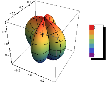
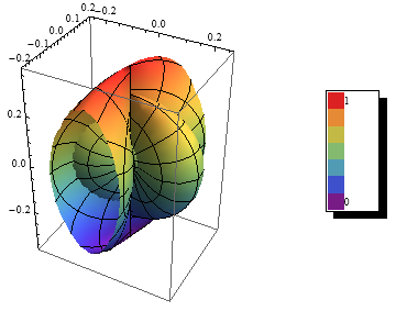
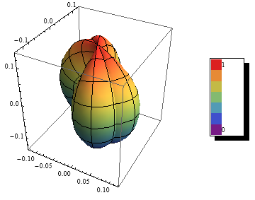
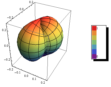
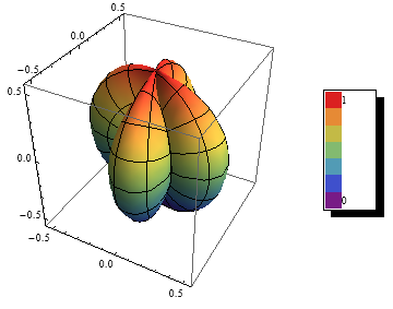
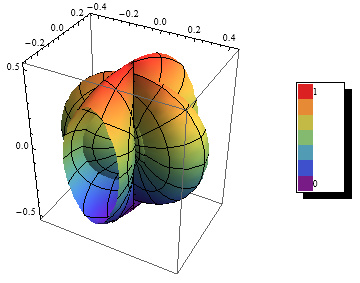
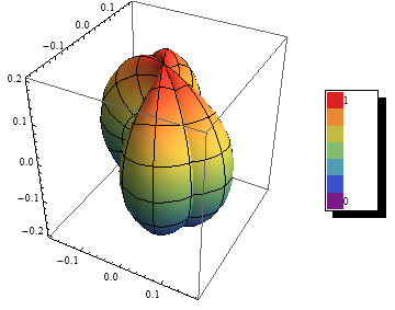
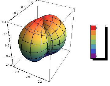
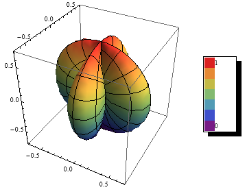
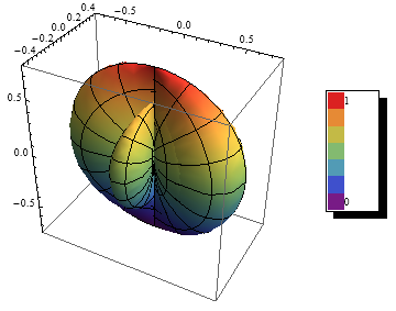
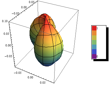
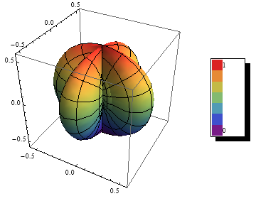
Figure 2: Beam pattern function for the massive wave as a function of $\phi$ and $\psi$ for the sources described in Table $1$ in their order, for the LIGO Hanford (left) and LIGO Livingston (right) respectively.

Fig. $(2)$ shows the beam pattern function behavior with the azimuth angle $\phi$ and the polarization angle $\psi$. The antenna patterns are in agreement with that proposed for massive scalar polarization component[30]. It can be easily inferred from the figure that the beam pattern function behaves in a highly directional manner towards an incoming wave of massive polarization which means that the detector could detect a massive component of GW polarization coming from a source only in a specific direction.

3 A Bayesian approach to signal detection

In this section, the Bayesian method is invoked to analyze the massive scalar polarization of GW signal emanated from a GRB that approaches the LIGO detector. Bayesian data analysis has already been done for the case of Pulsar timing arrays for the ${}^{\prime}+^{\prime}$ and ${}^{\prime}\times^{\prime}$ polarizations of GWs[39]. The study of Bayes factor as a norm for model selection, as to which model describes the data best is also studied in this section.

The Bayesian view is more general in which the probabilities provide a quantification of uncertainty ie., the result of Bayesian analysis is a quantitative measure, stating how far the chosen proposition is true. One advantage of the Bayesian viewpoint is that the inclusion of prior knowledge arises naturally. Bayesian analysis is completely controlled by the Bayesian law of conditional probabilities that include the sum rule and the product rule. The law is given by[40],

$$p(w|D)=\frac{p(D|w)p(w)}{p(D)},$$ (18)

where $D$ is the observed data, $w$ is the parameter that defines the proposition for $D$ and $p(w)$ is the prior probability. It is the probability available before we observe the data. $p(w|D)$ is called the posterior probability because it is the probability obtained after we observe the data. $p(D|w)$ is the likelihood function. It expresses how probable the observed data set is, for different elements of the parameter vector w. $p(D)$ is the normalization constant that makes the posterior distribution a valid one and also ensure that it integrates to $1$. Then, $p(D)$ can be written as,

$$p(D)=\int{p(D|w)p(w)dw}.$$ (19)

Applying the Bayesian approach to the GW signal analysis, we follow Finn and Lommen[39] to analyze the massive GWs from GRBs. Suppose that the observed data is $D$ and let $h$ be the proposed wave that describes the data $D$. The output data that we receive from a detector will be a mixture of the original waveform $h$ and the noise, $n$ of the detector, ie.,

$$D=h(t)+n(t),$$ (20)

where $h(t)$ is given by $(9)$. Here we deal only with the massive scalar mode. Assuming that the wave exhibits only a single mode at a time, the above equation can be written as,

$$D=F_{s}(\theta,\phi)h_{s}+n(t).$$ (21)

In this equation, we have taken $m=1$ for convenience. The noise is assumed to be a zero mean additive Gaussian noise. Then, the Bayesian law given by $(18)$ can be written in the form,

$$p(h|D)=\frac{\Lambda(D|h)p(h)}{p(D)},$$ (22)

where $p(h|D)$ is the posterior probability density, $\Lambda$ is the likelihood function, $p(h)$ is the prior probability density and $p(D)$, the normalization constant. The likelihood function $\Lambda$ can be written as[40]

$$\Lambda(h|D)=N(\textbf{D}-\textbf{F}_{s}\textbf{h}_{s}|\textbf{C}),$$ (23)

where $N$ denotes data drawn independently from a multivariate Gaussian distribution. C is the noise covariance and $N(x|C)$, for a multivariate normal distribution with zero mean random deviate $x$ given covariance C is given by,

$$N(x|C)=\frac{exp{(-\frac{1}{2}x^{T}C^{-1}x)}}{\sqrt{(2\pi)^{\mathcal{N}}det||C||}}$$ (24)

where $\mathcal{N}$ is the number of elements in vector $x$. Assuming that the a priori probability distribution is of Gaussian form, we can write,

$$\begin{split}p(h_{s})&=N(h_{s}|\sigma_{s}I)\\ &=[(2\pi\sigma_{s}^{2})]^{-1/2}exp{(-\frac{1}{2}\frac{h_{s}^{2}}{\sigma_{s}^{2}})},\end{split}$$ (25)

As already stated in Section $1$, the Bayesian non-parametric formulation depends on the dimension of the parameter space. Therefore, dimensionality should be included in the a priori distribution. The Gaussian distribution in higher dimensional space containing many input variables is then given by[39, 41, 42],

$$p(h_{s})=[(2\pi\sigma_{s}^{2})^{\mathcal{N}}]^{-1/2}exp{(-\frac{1}{2}\sum_{k=1}^{\mathcal{N}}\frac{h_{k}^{2}}{\sigma_{s}^{2}})},$$ (26)

where $\sigma_{s}$ is an undetermined constant, $\mathcal{N}$ can be treated as the number of data taken and $I$ denotes an appropriately dimensioned identity matrix. The normalization constant $p(D)$ is the integral of the product of the likelihood function and the a priori probability density over all possible values of $h_{s}$. Exploiting $(19)$, $(23)$, $(24)$ and $(25)$, we can write,

$$\begin{split}p(D)&=\int{\Lambda(h|D)p(h_{s})d^{\mathcal{N}}}h_{s}\\ &=\frac{exp{(-\frac{1}{2}[\textbf{h}(t)^{T}\textbf{C}^{-1}\textbf{h}(t)])}}{\sqrt{(2\pi)^{\mathcal{N}}det||C||}}\\ &\times\frac{exp{(\frac{1}{2}(F_{s}^{T}C^{-1}h(t))^{T}A^{-1}(F_{s}^{T}C^{-1}h(t)))}}{\sqrt{det||A||\sigma_{s}^{2\mathcal{N}}}},\end{split}$$ (27)

where A can be expressed as,

$$A=\sigma_{s}^{-2}I_{s}+F_{s}^{T}C^{-1}F_{s},$$ (28)

and $I_{s}$ is an appropriately dimensioned identity matrix.

Finally, the posterior probability density $p(h|D)$ can be written as,

$$p(h|D)=\sqrt{\frac{det||A||}{(2\pi)^{\mathcal{N}}}}exp{[\frac{1}{2}(h-h_{0})^{T}A(h-h_{0})]},$$ (29)

where $h_{0}$ satisfies,

$$Ah_{0}=F_{s}^{T}C^{-1}h(t).$$ (30)

It can be easily inferred from the above equation that $h_{0}$ is the waveform that maximizes the probability density $p(h_{s}|h(t))$. The amplitude Signal-to-Noise Ratio, $\rho$ associated with $h_{0}$ is given by

$$\rho^{2}=(F_{s}h_{0})^{T}C^{-1}(F_{s}h_{0}).$$ (31)

Finally, the quantity Bayes Factor helps us to decide on whether a signal is present or not. It chooses between different models. For any observations D, the Bayes factor for $M_{1}$ against $M_{0}$ is defined by[43, 44],

$$B_{10} = \frac{m_{1}(\theta)}{m_{0}(\theta)}$$ (32)

$$= \frac{p(D|M_{1})}{p(D|M_{0})},$$ (33)

$\theta$ is some unknown parameter. The probability given in $(33)$ is nothing but the likelihood function. Therefore, employing the form of $(23)$,

$$p(D|M_{1})=\Lambda(D|M_{1},h_{s},\sigma_{s}),$$ (34)

gives the probability density of observations $D$ assuming the GW signal described by parameter $\sigma_{s}$ is present,

$$p(D|M_{0})=\Lambda(D|M_{0}),$$ (35)

gives the probability density of $D$ assuming no signal is present. The Bayes factor can then be written as[39],

$$B_{(D)}=\int{\frac{d^{2}\Omega_{k}}{4\pi}\frac{exp{(-\frac{1}{2}[\textbf{D}^{T}\textbf{C}^{-1}\textbf{D}])}}{\sqrt{det|A|\sigma_{s}^{2dimh_{s}}}}}.$$ (36)

Now, from Bayes theorem, the posterior probability of model $M_{1}$ can be expressed through Bayes factor as[43]

$$p(M_{1}|D) = \frac{p(M_{1})m_{1}(D)}{p(M_{1})m_{1}(D)+p(M_{0})m_{0}(D)}$$ (37)

$$= \frac{p(M_{1})B_{10}}{p(M_{0})+p(M_{1})B_{10}},$$ (38)

where $p(M_{i})$ is the prior probability of model $M_{i}$ for $i=0$. In the absence of any prior knowledge, $p(M_{0})=p(M_{1})=1/2$. Therefore, the model $M_{1}$ is more likely to be chosen if $p(M_{1}|D)>\frac{1}{2}$ or equivalently $B_{10}>1$.

Thus, Bayes factor is always positive. On the average, Bayes factor will always favor the correct model. A Bayes factor large compared to unity favor $M_{1}$ and a Bayes factor small compared to unity favor the model $M_{0}$.

3.1 Methodology

Firstly, in order to check the possibility of detecting massive GW in the LIGO, the simulated data from $(21)$ is used. For that, a simplest adhoc waveform given by a Gaussian distribution is used for $h_{s}$, and can be written as in Abbott et al.[45],

$$h_{s}(t+t_{0})=h_{s,0}(\omega_{m})\cos{(2\pi f_{0}t)}\exp(-\frac{(2\pi f_{0}t)^{2}}{2Q^{2}}),$$ (39)

where $t_{0}$ is the central time, $f_{0}$ is the central frequency, which is taken in the range of $0$ to $200$Hz; $h_{s,0}$ is the amplitude parameter that is characterized by $\omega_{m}$ of $(4)$ and is given as[28, 29],

$$\omega_{m}=\frac{m}{\sqrt{1-v_{g}^{2}}},$$ (40)

where $m$ is the mass corresponding to the additional scalar mode of GW polarization, $v_{g}$ is the velocity of propagation of GW and $Q$ is a dimensionless constant which represents roughly the number of cycles with which the waveform oscillates more than half of the peak amplitude. A standard choice in LIGO burst searches for $Q$ is $8.9$. $t$ will be very short and is taken in the range $0$ to $1$s. $h_{s,0}$ is given by[11],

$$h_{s,0}=\frac{1}{r}\sqrt{\frac{5GE_{GW}}{c^{3}Qf_{0}4.\pi^{3/2}}}$$ (41)

As an example to check whether massive scalar polarization resulting from metric $f(R)$ gravity will be detected, we take the random sample GRB$070201$. In order to simulate the detector output signal, $(41)$ is substituted in $(39)$. This in turn is substituted in $(21)$. For this candidate $E_{GW}=1.14\times 10^{-4}M_{\odot}c^{2}$ and $r=770$Kpc[46]. Taking $F_{s}$ from $(17)$ and noise from the LIGO Scientific Collaboration[47], the simulated waveform for different values of $m$ are shown in Fig. $4$.

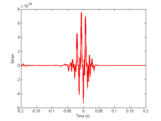
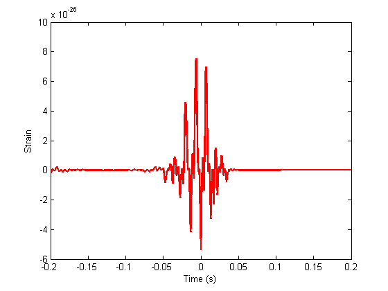
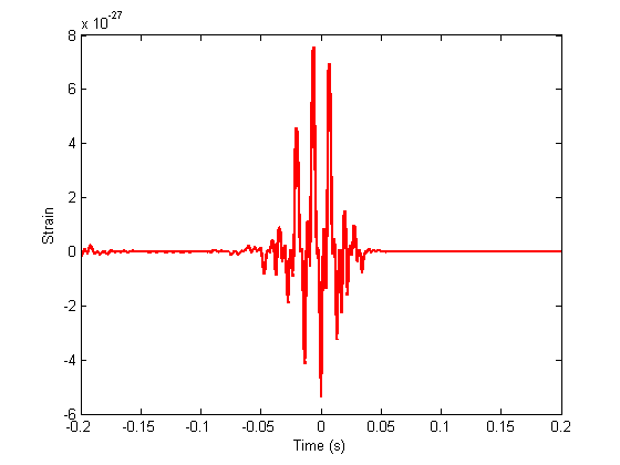
Figure 3: The simulated output signal for GRB070201 for $m=1$, $m=1\times 10^{-21}$,$m=1\times 10^{-22}$ and $m=1\times 10^{-23}eV/c^{2}$ from top left

The data used in this section for Bayesian analysis is taken from this simulated output waveform. Also, the predicted waveform is taken from $(39)$. Even though it is not the wisest choice, it will serve the purpose of the present work. After having the data $D$ and the predicted waveform $h_{s}$, the parameter $\sigma_{s}$ is to be estimated in order to get the most probable waveform and also the Bayes factor. This is done by the optimization of $(27)$ with respect to $\sigma_{s}$. While optimizing, maximization is used since it is more favored[48]. The equation as such is too complicated to optimize and therefore it is simplified by taking the logarithm of $p(D)$. This procedure is fully justified since logarithm is a monotonically increasing function of its argument. So, maximizing $\log{p(D)}$ with respect to $\sigma_{s}$ is equivalent to maximizing $p(D)$. Thus $(27)$ becomes :

$$\begin{split}\log{p(D)}&=\log{[\frac{exp{-\frac{1}{2}[\textbf{h}(t)^{T}\textbf{C}^{-1}\textbf{h}(t)]}}{\sqrt{(2\pi)^{dimx}det||C||}}]}\\ &+\log{[\frac{exp{\frac{1}{2}(F_{s}^{T}C^{-1}h(t))^{T}A^{-1}(F_{s}^{T}C^{-1}h(t))}}{\sqrt{det||A||\sigma_{s}^{2dimh_{s}}}}]}.\end{split}$$ (42)

Since we are maximizing with respect to $\sigma_{s}$, the first term on the right hand side can be suitably omitted as it is independent of $\sigma_{s}$. The second term is optimized. Using the values of matrix A that is got by optimizing, $(30)$ is simultaneously solved for $\textbf{h}_{0}$, the most probable waveform (inferred waveform) for the given data. After getting $\textbf{h}_{0}$, the signal to noise ratio $(\rho)$ can be calculated using $(31)$. Then the Bayes factor can be evaluated using $(36)$.

3.2 Results

The possible bounds on the mass of graviton corresponding to different theories of gravity is discussed in the work of de Rham et al.[49]. Bounds from the direct GW detection limit the graviton mass as[7] $m_{g}<1.2\times 10^{-22}\,eV/c^{2}$. Invoking these bounds, using the method discussed in the previous subsection, the optimization is done by choosing the mass corresponding to the additional scalar mode of GW polarizations as $m=10^{-21},\,10^{-22}$ and $10^{-23}\,eV/c^{2}$. The results are shown in Table $2$.

Table $2$ : Results showing the calculation of log of Bayes factor and SNR for different values of $m$.

$m(eV/c^{2})$ $\sigma_{s}$ $\rho$ $lnB_{D}$ signal $10^{-21}$ $1\times 10^{-11}$ $\sim 0.1360$ $\sim-1.7\times 10^{3}$ weak/Absent $10^{-22}$ $1\times 10^{-11}$ $\sim 0.1360$ $\sim-1.7\times 10^{3}$ weak/Absent $10^{-23}$ $1\times 10^{-11}$ $\sim 0.1360$ $\sim-1.7\times 10^{3}$ weak/Absent

It can be seen that there is not much change in the values of Bayes factor and SNR with the change in the mass of the scalar mode of polarization in the range shown in the table. Comparing the values of the Bayes factor and SNR given in Table $2$ with those in Table $2$ of the Ref. $[39]$, it can be seen that the Bayes factor and SNR values are very low indicating an absence of the signal. Thus it can be concluded that with the given sensitivity and orientation of the LIGO detector, a massive scalar polarization from $f(R)$ theory with a value of mass in the range $m=1\times 10^{-21}$ to $1\times 10^{-23}eV/c^{2}$ is unlikely to be detected. The comparison of most probable waveform with the actual one is shown in Fig. $4$. This null result can be compared with the results obtained in the works of Aasi et al.[50] and Xihao Deng[51] where they predicted null results for GRBs in the case of $+$ and $\times$ polarization with the existing observational set up.

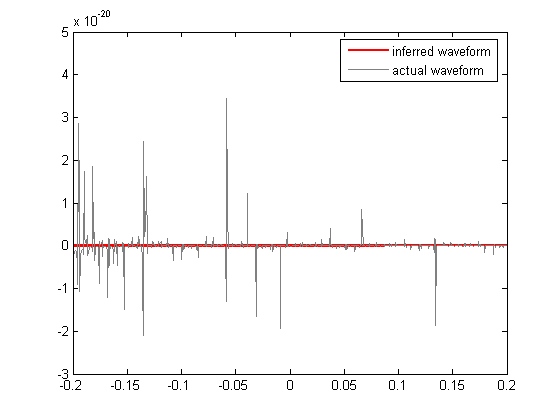
Figure 4: Comparison of the inferred and the actual waveforms for the LIGO detector for $m=1\times 10^{-21}$ on the top and for $m=1\times 10^{-22},\,1\times 10^{-23}$ respectively from left on the bottom row.

4 Conclusion

We have considered the production of massive GWs from a metric $f(R)$ theory of gravity and the beam pattern it produces on an interferometer detector. We have calculated the specific form for the interferometer antenna response function in the detector coordinates for the massive GWs. These are then considered for the cases of LIGO Hanford and Livingston detectors for seven Gamma Ray Burst (GRB) sources. These sources are selected at random. It is found that the beam pattern functions are highly directional. They are sensitive to the direction in which the wave comes. A Bayesian analysis has been done to check the possibility of detecting a massive scalar component of GW polarizations from the source GRB 070201 using simulated data for LIGO, for the values of masses: $m=10^{-21},10^{-22}$ and $10^{-23}eV/c^{2}$. The parameter of the predicted waveform, which is nothing but the rms amplitude of the wave, is determined by optimization method. The Bayes factor and the SNR values are also determined. For all the cases the analysis gave low values of SNR and Bayes factor. Thus with the model discussed in this work for a GRB event and the beam pattern function, the massive polarization is not likely to be detected. The results are prone to change with a different a priori waveform. Even though the results presented in this paper are not conclusive enough, it gives insight in to the study of GWs from alternative theories or extended theories of gravity.

5 Acknowledgements

The authors would like to thank the reviewer for the comments for the improvement of the paper. One of us (PP) would like to thank UGC, New Delhi for financial support through the award of a Junior Research Fellowship (JRF) during the period $2010$-$2013$. PP would also like to acknowledge Govt. College, Chittur for allowing to pursue her research. VCK would like to acknowledge Associateship of IUCAA, Pune.

References

- [1] S. Capozziello and V. Faraoni, Beyond Einstein Gravity (Springer, 2011).
- [2] Thomas P. Sotiriou and V. Faraoni, Rev. Mod. Phys., 82 (2010) 451.
- [3] de Rham C., Gregory Gabadadze and Andrew J. Tolley, Phys. Rev. Lett., 106 (2011) 231101.
- [4] de Rham C., Living Rev. Relativity, 17 (2014) 7.
- [5] R. P. Woodard, Lect. Notes Phys. 720 (2007) 403.
- [6] Enna E. Flanagan and Scott A. Hughes, New. J. Phys., 7 (2005) 204.
- [7] B. P. Abbott et al., Phys. Rev. Lett., 116 (2016) 061102.
- [8] B. P. Abbott et al., Phys. Rev. Lett., 116 (2016) 241103.
- [9] B. P. Abbott et al., Phys. Rev. D, 80 (2009) 102001.
- [10] B. P. Abbott et al., ApJ, 715 (2010) 1438.
- [11] J. Abadie et al., ApJ, 760 (2012) 1.
- [12] D. Eichler, M. Livio, T. Piran, and D. N. Schramm, Nature (London) 340 (1989) 126.
- [13] B. Paczynski, Acta Astronomica, 41 (1991) 257.
- [14] S. E. Woosley, Astrophys. J. 405 (1993) 273.
- [15] Kobayashi S. and Meszaros P., ApJ, 589 (2003) 861.
- [16] Abadie J. et al., Classical and Quantum Gravity, 27 (2010) 173001.
- [17] B. P. Abbott et al., Phys. Rev. Lett., 116 (2016) 221101.
- [18] C. M. Will, Living Rev. Rel., 17 (2014) 4.
- [19] A. Emir Gumrukcuoglu et al., Class. Quantum Grav. 29 (2012) 235026.
- [20] Yunes N. & Siemens X., Living Rev. Relativity, 16, (2013), 9.
- [21] Berti E. et al., Class. Quantum Grav. 32 (2015) 243001.
- [22] Lixin Xu, Phys. Rev. D, 91 (2015) 103520.
- [23] M. Maggiore, Gravitational Waves, Vol. 1 (Oxford, 2008).
- [24] L. S. Finn, Issues in gravitational wave data analysis (1997) arXiv:gr-qc/9709077.
- [25] A. Gelman, J. B. Carlin, H. S. Stern, and D. B. Rubin, Bayesian Data Analysis, 2nd ed., Texts in Statistical Science (Chapman & Hall/CRC, 2004).
- [26] Orbanz Peter and M. Roy Daniel, IEEE Transactions Pattern Analysis and Machine Intelligence, 37 (2015) 437.
- [27] C. Corda, Gen. Relativ Gravit., 40 (2008) 2201.
- [28] S. Capozziello et al., Eur. Phys. J. C, 70 (2010) 341.
- [29] P. Prasia and V. C. Kuriakose, Int. J. Mod. Phys. D, 23 (2014) 1450037.
- [30] M. Maggiore and A. Nicolis, Phys. Rev. D, 62 024004.
- [31] Emil Mottola, Scalar Gravitational Waves in the Effective Theory of Gravity, arXiv:1606.09220 [gr-qc] (2016) LA-UR-16-23649.
- [32] M. E. S. Alves, O. D. Miranda and J. C. N. de Araujo, Phys. Lett. B, 679 (2009) 401.
- [33] H. Rizwana Kausar, Lionel Philippoz and Philippe Jetzer, Phys. Rev. D, 93 (2016) 124071.
- [34] M. E. S. Alves, O. D. Miranda and J. C. N. de Araujo, Class. Quantum Grav., 27 (2010) 145010.
- [35] P. Jaranowski and A. Krolak, Phy. Rev. D, 49 (1994) 1723.
- [36] P. Jaranowski, A. Krolak and B. F. Schutz, Phy. Rev. D, 58 (1998) 063001.
- [37] J. Abadie et al., ApJ, 760 (2012) 12.
- [38] B. P. Abbott et al., ApJ, 715:1438 1452 (2010).
- [39] L. S. Finn and A. N. Lommen, ApJ, 718 (2010) 1400.
- [40] Bishop C. M., Pattern Recognition and Machine Learning (Springer, 2006).
- [41] L. S. Finn, Phys. Rev. D, 79 (2009) 022002.
- [42] Wang Min and Sun Xiaoqian, J. Stat. Plan. Inference, 147 (2014) 95.
- [43] A. F. N. Smith and D. J. Spiegelhalter, J. R. Statist. Soc. B, 42 (1980) 2, 213.
- [44] Wang Min and Sun Xiaoqian, Commun. Stat. Theory, 43 (2014) 5072.
- [45] B. P. Abbott et al., Rep. Prog. Phys., 72 (2009) 076901.
- [46] B. P. Abbott et al., Phys. Rev. D, 77 (2008) 062004.
- [47] LIGO Scientific Collaboration, “LIGO Open Science Center release of S5” (2014) DOI 10.7935/K5WD3XHR.
- [48] J. C. MacKay David, Neural Computation, 4 (1992) 415.
- [49] de Rham C. et al., Graviton Mass Bounds, arXiv:1606.08462 [astro-ph.CO] (2016).
- [50] J. Aasai et al., Phys. Rev. Lett., 113 (2014) 011102.
- [51] Xihao Deng, Phy. Rev. D, 90 (2014) 024020.