Quantum quench of the Sachdev-Ye-Kitaev Model

Abstract

We describe the non-equilibrium quench dynamics of the Sachdev-Ye-Kitaev models of fermions with random all-to-all interactions. These provide tractable models of the dynamics of quantum systems without quasiparticle excitations. The Kadanoff-Baym equations show that the final state is thermal, and their numerical analysis is consistent with a thermalization rate proportional to the absolute temperature of the final state. We also obtain an exact analytic solution of the quench dynamics in the large $q$ limit of a model with $q$ fermion interactions: in this limit, the thermalization of the fermion Green’s function is instantaneous.

I Introduction

The non-equilibrium dynamics of strongly interacting quantum many-particle systems have been the focus of much theoretical work Kamenev (2013). These are usually studied within the Schwinger-Keldysh formalism, which can describe evolution from a generic initial state to a final state which reaches thermal equilibrium at long times. The thermodynamic parameters of the final state (e.g. temperature) are determined by the values of the conjugate conserved quantities (e.g. energy). The Kadanoff-Baym equations obtained from this formalism describe the manner and rate by which this final thermal state is reached.

The Kadanoff-Baym equations are usually too difficult to solve in their full generality. Frequently, a quasiparticle structure has been imposed on the spectral functions, so that the Kadanoff-Baym equations reduce to a quantum Boltzmann equation for the quasiparticle distribution functions. Clearly such an approach cannot be employed for final states of Hamiltonians which describe critical quantum matter without quasiparticle excitations. The most common approach is then to employ an expansion away from a regime where quasiparticles exist, using a small parameter such as the deviation of dimensionality from the critical dimension, or the inverse of the number of field components: the analysis is then still carried out using quasiparticle distribution functions Damle and Sachdev (1997); Sachdev (1998).

In this paper, we will examine the non-equilibrium dynamics towards a final state without quasiparticles. We will not employ a quasiparticle decomposition, and instead provide solutions of the full Kadanoff-Baym equations. We can obtain non-equilibrium solutions for the Sachdev-Ye-Kitaev (SYK) models Sachdev and Ye (1993); Kitaev (2015); Maldacena and Stanford (2016) with all-to-all and random interactions between $q$ Majorana fermions on $N$ sites. These models are solvable realizations of quantum matter without quasiparticles in equilibrium, and here we shall extend their study to non-equilibrium dynamics. We shall present numerical solutions of the Kadanoff-Baym equations for the fermion Green’s function at $q=4$, and in Section IV, an exact analytic solutions in the limit of large $q$ (no quasiparticles are present in this limit). The large $q$ solution relies on a remarkable exact SL(2,C) invariance, and has connections to quantum gravity on AdS₂ with the Schwarzian effective action Sachdev (2010a, b); Almheiri and Polchinski (2015); Kitaev (2015); Maldacena and Stanford (2016); Jensen (2016); Engelsöy et al. (2016) for the equilibrium dynamics, as we will note in Section V.

The equilibrium SYK Hamiltonian we shall study is (using conventions from Ref. Maldacena and Stanford, 2016)

$$H=(i)^{\frac{q}{2}}\sum_{1\leq i_{1}<i_{2}<...<i_{q}\leq N}j_{i_{1}i_{2}...i_{q}}\psi_{i_{1}}\psi_{i_{2}}...\psi_{i_{q}}$$ (1)

where $\psi_{i}$ are Majorana fermions on sites $i=1\ldots N$ obeying

$$\{\psi_{i},\psi_{j}\}=\delta_{ij}\,,$$ (2)

and $j_{i_{1}i_{2}...i_{q}}$ are Gaussian random variables with zero mean and variance

$$\langle j^{2}_{i_{1}...i_{q}}\rangle=\frac{J^{2}(q-1)!}{N^{q-1}}.$$ (3)

Our numerical analysis of the SYK model will be carried out on the case with time-dependent $q=2$ and $q=4$ terms:

$$H(t)=i\sum_{i<j}j_{2,ij}\,f(t)\,\psi_{i}\psi_{j}-\sum_{i<j<k<l}j_{4,ijkl}\,g(t)\,\psi_{i}\psi_{j}\psi_{k}\psi_{l},$$ (4)

where $j_{2,ij}$ and $j_{4,ijkl}$ are random variables as described above, and $f(t)$ and $g(t)$ can be arbitrary functions of time. We will focus on a particular quench protocol in which

$$\mbox{for $t<0$, $f(t)=1$ and $g(t)=1$}\,;$$

$$\mbox{for $t>0$, $f(t)=0$ and $g(t)=1$}\,.$$ (5)

For $t<0$, we have a thermal initial state with both $q=2$ and $q=4$ interactions present. In this case the $q=2$ free fermion terms dominate at low energies, and hence we have Fermi liquid behavior at low temperatures. For $t>0$, we have only the $q=4$ Hamiltonian as in Eq. (1), which describes a non-Fermi liquid even at the lowest energies Sachdev and Ye (1993). Just after the quench at $t=0$, the system is in a non-equilibrium state. We show from the Kadanoff-Baym equations, and verify by our numerical analysis, that the $t\rightarrow\infty$ state is indeed a thermal non-Fermi liquid state at $q=4$, which is at an inverse temperature $\beta_{f}=1/T_{f}$. The value of $\beta_{f}$ is such that the total energy of the system remains the same after the quench at $t=0^{+}$.

We note in passing that an alternative quench protocol in which $f(t)=0$ for all $t$, while $g(t)$ is time dependent (or the complementary case in which $g(t)=0$ for all $t$, while $f(t)$ is time-dependent), does not yield any non-trivial dynamics (this was pointed out to us by J. Maldacena). This case corresponds to an overall rescaling of the Hamiltonian, which does not change any of the wavefunctions of the eigenstates. So an initial state in thermal equilibrium will evolve simply via a time reparameterization which is given in Eq. (54).

We will describe the time evolution of the system for $t\geq 0$ by computing a number of two-point fermion Green’s functions $G(t_{1},t_{2})$. As the system approaches thermal equilibrium, it is useful to characterize this correlator by

$$\mathcal{T}=(t_{1}+t_{2})/2\quad,\quad t=t_{1}-t_{2}\,.$$ (6)

Then we have

$$\lim_{\mathcal{T}\rightarrow\infty}G(t_{1},t_{2})=G_{\beta_{f}}(t)$$ (7)

where $G_{\beta_{f}}$ is the correlator in equilibrium at an inverse temperature $\beta_{f}$. For large $\mathcal{T}$ we will characterize $G(t_{1},t_{2})$ by an effective temperature $\beta_{\rm eff}(\mathcal{T})$ (see below). From our numerical analysis we characterize the late time approach to equilibrium by

$$\beta_{\text{eff}}(\mathcal{T})=\beta_{f}+\alpha\exp\left(-\Gamma\mathcal{T}\right)\,.$$ (8)

This defines a thermalization rate, $\Gamma$. Our complete numerical results for $\Gamma$ appear in Fig. 7, and they are reasonably fit to the behavior

$$\Gamma=C/\beta_{f}\quad,\quad\beta_{f}J_{4}\gg 1\,,$$ (9)

where $C$ is a numerical constant independent of the initial state. Thus, at low final temperatures, the thermalization rate of the non-Fermi liquid state appears proportional to temperature, as is expected for systems without quasiparticle excitations Sachdev (1999).

I.1 Large $q$ limit

Further, we will also consider a model in which the $t<0$ Hamiltonian has a $q$-fermion interaction $\mathcal{J}$, and a $pq$ fermion interaction $\mathcal{J}_{p}$. At $t>0$ we then quench to only a $q$ fermion interaction $\mathcal{J}$. We will show that the non-equilibrium dynamics of this model are exactly solvable in the limit of large $q$ taken at fixed $p$.

The large $q$ Green’s function can be written as Maldacena and Stanford (2016)

$$G^{>}(t_{1},t_{2})=-i\left\langle\psi(t_{1})\psi(t_{2})\right\rangle=-\frac{i}{2}\left[1+\frac{1}{q}g(t_{1},t_{2})+\ldots\right]$$ (10)

where

$$g(t,t)=0\,.$$ (11)

For $t_{1}>0$ or $t_{2}>0$, we find that $g(t_{1},t_{2})$ obeys the two-dimensional Liouville equation

$$\frac{\partial^{2}}{\partial t_{1}\partial t_{2}}g(t_{1},t_{2})=2\mathcal{J}^{2}\,e^{g(t_{1},t_{2})}\,,$$ (12)

where $\mathcal{J}$ is proportional to the final interaction strength (see Eq. (56)). The most general solution of this equation can be written as Tsutsumi (1980)

$$g(t_{1},t_{2})=\ln\left[\frac{-h_{1}^{\prime}(t_{1})h_{2}^{\prime}(t_{2})}{\mathcal{J}^{2}(h_{1}(t_{1})-h_{2}(t_{2}))^{2}}\right]\,,$$ (13)

where $h_{1}(t_{1})$ and $h_{2}(t_{2})$ are arbitrary functions of their arguments. A remarkable and significant feature of this expression for $g(t_{1},t_{2})$ is that it is exactly invariant under SL(2,C) transformations

$$h_{\alpha}(t)\rightarrow\frac{a\,h_{\alpha}(t)+b}{c\,h_{\alpha}(t)+d}\,,$$ (14)

where $\alpha=1,2$ and $a,b,c,d$ are arbitrary complex numbers. We will use the Schwinger-Keldysh analysis to derive ordinary differential equations that are obeyed by $h_{1,2}(t)$ in Section IV. Naturally, these equations will also be invariant under SL(2,C) transformations. We will show that for generic initial conditions in the regime $t_{1}<0$ and $t_{2}<0$, the solutions for $h_{1}(t_{1})$ and $h_{2}(t_{2})$ at $t_{1}>0$ and $t_{2}>0$ can be written as

$$h_{1}(t)=\frac{a\,e^{i\theta}e^{\sigma t}+b}{c\,e^{i\theta}e^{\sigma t}+d}\quad,\quad h_{2}(t)=\frac{a\,e^{-i\theta}e^{\sigma t}+b}{c\,e^{-i\theta}e^{\sigma t}+d}\,.$$ (15)

The complex constants $a,b,c,d$, and the real constants $\sigma$, $\theta$ are determined by the initial conditions in the $t_{1}<0$ and $t_{2}<0$ quadrant of the $t_{1}$-$t_{2}$ plane. Note that we pick a particular SL(2,C) orientation in the $t_{1}\leq 0$, $t_{2}\leq 0$ quadrant, and then there is no further SL(2,C) arbitrariness in the $t_{1}>0$, $t_{2}>0$ quadrant. Inserting Eq. (15) into Eqs. (11,13) at $t_{1}=t_{2}$, we obtain

$$\sigma=2\mathcal{J}\sin(\theta)\,.$$ (16)

For general $t_{1}>0$ and $t_{2}>0$, inserting Eq. (15) into Eq. (13) we obtain

$$g(t_{1},t_{2})=\ln\left[\frac{-\sigma^{2}}{4\mathcal{J}^{2}\sinh^{2}(\sigma(t_{1}-t_{2})/2+i\theta)}\right]\,.$$ (17)

The surprising feature of this result is that it depends only upon $t=t_{1}-t_{2}$, and is independent of $\mathcal{T}=(t_{1}+t_{2})/2$. Indeed Eq. (17) describes a state in thermal equilibrium Parcollet and Georges (1999); Maldacena and Stanford (2016) at an inverse temperature

$$\beta_{f}=\frac{2(\pi-2\theta)}{\sigma}\,.$$ (18)

So the large $q$ limit yields a solution in which the fermion Green’s function thermalizes instantaneously at $t=0^{+}$ at the final temperature given by Eq. (18). This could indicate that the thermalization rate $\Gamma$ diverges as at $q\rightarrow\infty$. Alternatively, as pointed out to us by Aavishkar Patel, the present large $q$ solution could describe a pre-thermal state, and the $1/q^{2}$ corrections in Eq. (10) have a finite thermalization rate; in such a scenario, thermalization is a two-step process, with the first step occuring much faster than the second. But we will not examine the $1/q^{2}$ corrections here to settle this issue.

Note also that in the limit $\beta_{f}\mathcal{J}\gg 1$, we have $\theta\ll 1$ and then

$$\sigma=\frac{2\pi}{\beta_{f}}\,.$$ (19)

Then Eqs. (10) and (17) describe the $1/q$ expansion of the low temperature conformal solution Parcollet and Georges (1999) describing the equilibrium non-Fermi liquid state (see Appendix B). And the value of $\sigma$ in Eq. (19) is the maximal Lyapunov exponent for quantum chaos Maldacena et al. (2016). This chaos exponent appears in the time evolution of $h_{1,2}(t)$. However, in the large $q$ limit, it does not directly control the rapid thermalization rate. We note that recent studies of Fermi surfaces coupled to gauge fields, and of disordered metals, found a relaxation/dephasing rate which was larger than the Lyapunov rate Patel and Sachdev (2017); Patel et al. (2017).

We will begin by setting up the Schwinger-Keldysh formalism for Majorana fermions in the SYK model in Sections II. The numerical solution of the Kadanoff-Baym equations appears in Section III. Finally, the large $q$ limit is described in Section IV.

II Kadanoff-Baym equations from the path integral

We construct the path integral for Majorana fermions from the familiar complex fermion path integral Sedrakyan and Galitski (2011) by expressing the complex fermions $\Psi_{i}$ in terms of two real fermions $\psi_{i}$ and $\chi_{i}$ i.e. $\Psi_{i}=\psi_{i}+i\chi_{i}$. Since $\chi_{i}$ is just a spectator which does not appear in the Hamiltonian, we can disregard its contribution and write down the path integral representation of the partition function as

$$Z=\int\mathcal{D}\psi e^{iS[\psi]}$$ (20)

with the action

$$\begin{split}S[\psi]&=\int_{\mathcal{C}}dt\Bigl{\{}\frac{i}{2}\sum_{i}\psi_{i}\partial_{t}\psi_{i}-i\sum_{i<j}j_{2,ij}f(t)\psi_{i}\psi_{j}+\sum_{i<j<k<l}j_{4,ijkl}g(t)\psi_{i}\psi_{j}\psi_{k}\psi_{l}\Bigr{\}}\,.\end{split}$$ (21)

Here, the Majorana fields $\psi_{i}$ live on the closed time contour $\mathcal{C}$, also known as Schwinger-Keldysh contour. In order to include the disorder, we average the partition function over Gaussian distributed couplings as

$$Z=\int D\psi\int Dj_{2,ij}\int Dj_{4,ijkl}P(j_{4,ijkl})P(j_{2,ij})e^{iS[\psi]}\,,$$ (22)

where the probability distributions are given by

$$\mathcal{P}_{1}(j_{2,ij})=\sqrt{\frac{N}{2J_{2}^{2}\pi}}\operatorname{exp}\Big{(}-\frac{N}{2J_{2}^{2}}\sum_{i<j}j_{2,ij}^{2}\Big{)},$$ (23)

$$\mathcal{P}_{2}(j_{4,ijkl})=\sqrt{\frac{N^{3}}{12J_{4}^{2}\pi}}\operatorname{exp}\Big{(}-\frac{N^{3}}{12J_{4}^{2}}\sum_{i<j<k<l}j^{2}_{4,ijkl}\Big{)}.$$ (24)

This realization of disorder allows us to perform the integrals with respect to $j_{2,ij}$ and $j_{4,ijkl}$. The Gaussian integrals lead to

$$\begin{split}Z=\int D\psi\operatorname{exp}\Bigl{\{}&-\frac{1}{2}\int_{\mathcal{C}}dt_{1}\sum_{i}\psi_{i}\partial_{t_{1}}\psi_{i}-\frac{J_{2}^{2}}{4N}\sum_{i,j}\int_{\mathcal{C}}dt_{1}\int_{\mathcal{C}}dt_{2}f(t_{1})f(t_{2})\psi_{i}(t_{1})\psi_{i}(t_{2})\psi_{j}(t_{1})\psi_{j}(t_{2})\\ &-\frac{3J_{4}^{2}}{4!N^{3}}\sum_{i,j,k,l}\int_{\mathcal{C}}dt_{1}\int_{\mathcal{C}}dt_{2}g(t_{1})g(t_{2})\psi_{i}(t_{1})\psi_{i}(t_{2})\psi_{j}(t_{1})\psi_{j}(t_{2})\psi_{k}(t_{1})\psi_{k}(t_{2})\psi_{l}(t_{1})\psi_{l}(t_{2})\Bigr{\}}.\end{split}$$

We introduce the bilinear $G$, which must fulfill the constraint

$$G(t_{1},t_{2})=-\frac{i}{N}\sum_{i}\psi_{i}(t_{1})\psi_{i}(t_{2})\,.$$ (25)

To implement this constraint, we introduce the Lagrange multiplier $\Sigma$ leading to

$$\begin{split}Z=&\int D\psi\int DG\int D\Sigma\operatorname{exp}\Bigl{\{}-\frac{1}{2}\int_{\mathcal{C}}dt_{1}\sum_{i}\psi_{i}\partial_{t_{1}}\psi_{i}+\frac{J_{2}^{2}N}{4}\int_{\mathcal{C}}dt_{1}\int_{\mathcal{C}}dt_{2}f(t_{1})f(t_{2})G(t_{1},t_{2})^{2}\\ &-\frac{3J_{4}^{2}N}{4!}\int_{\mathcal{C}}dt_{1}\int_{\mathcal{C}}dt_{2}g(t_{1})g(t_{2})G(t_{1},t_{2})^{4}+\frac{i}{2}\int_{\mathcal{C}}dt_{1}\int_{\mathcal{C}}dt_{1}\Sigma(t_{1},t_{2})\bigl{[}G(t_{1},t_{2})+\frac{i}{N}\sum_{i}\psi_{i}(t_{1})\psi_{i}(t_{2})\bigr{]}\Bigr{\}}.\end{split}$$

Rescaling integration variables as $\Sigma\rightarrow iN\Sigma$ and integrating over $\psi$ yields

$$\begin{split}Z=&\int DG\int D\Sigma\operatorname{exp}\Bigl{\{}iS\bigl{[}G,\Sigma\bigr{]}\Bigr{\}}\end{split}$$ (26)

with

$$\begin{split}S\bigl{[}G,\Sigma\bigr{]}=&-\frac{iN}{2}\operatorname{tr}\operatorname{log}\bigl{[}-i(G_{0}^{-1}-\Sigma)\bigr{]}-\frac{iJ_{2}^{2}N}{4}\int_{\mathcal{C}}dt_{1}\int_{\mathcal{C}}dt_{2}f(t_{1})f(t_{2})G(t_{1},t_{2})^{2}\\ &+\frac{3iJ_{4}^{2}N}{4!}\int_{\mathcal{C}}dt_{1}\int_{\mathcal{C}}dt_{2}g(t_{1})g(t_{2})G(t_{1},t_{2})^{4}+\frac{iN}{2}\int_{\mathcal{C}}dt_{1}\int_{\mathcal{C}}dt_{2}\Sigma(t_{1},t_{2})G(t_{1},t_{2})\end{split}$$ (27)

and the free Majorana Green’s function $G_{0}^{-1}(t_{1},t_{2})=i\partial_{t}\delta_{\mathcal{C}}(t_{1},t_{2})$. ​Varying the action with respect to $\Sigma$ and $G$ yields the Dyson equation and the the self-energy, respectively:

$$G_{0}^{-1}(t_{1},t_{2})-G^{-1}(t_{1},t_{2}) =\Sigma(t_{1},t_{2})\,,$$ (28)

$$\Sigma(t_{1},t_{2}) =J_{2}^{2}f(t_{1})f(t_{2})G(t_{1},t_{2})-J_{4}^{2}g(t_{1})g(t_{2})G(t_{1},t_{2})^{3}.$$ (29)

Note that the time arguments are with respect to the full time contour, and the matrix structure of the Keldysh formalism is implicit. We define the following two Green’s functions

$$G^{>}(t_{1},t_{2}) \equiv G(t^{-}_{1},t^{+}_{2})\,,$$ (30a)

$$G^{<}(t_{1},t_{2}) \equiv G(t^{+}_{1},t^{-}_{2})\,$$ (30b)

where $t_{i}^{-}$ lives on the lower contour and $t_{i}^{+}$ lives on the upper contour In the case for Majorana fermions there is only one independent component of the Green’s function, even in non-equilibrium, due to the relation Babadi et al. (2015)

$$G^{>}(t_{1},t_{2})=-G^{<}(t_{2},t_{1}).$$ (31)

The bare greater and lesser Green’s functions are given by

$$G^{>}_{0}(t_{1},t_{2}) =-\frac{i}{2}\,.$$ (32)

We now use $G^{>}$ and $G^{<}$ to obtain the retarded, advanced and Keldysh Green’s functions:

$$G^{R}(t_{1},t_{2}) \equiv\Theta(t_{1}-t_{2})\bigl{[}G^{>}(t_{1},t_{2})-G^{<}(t_{1},t_{2})\bigr{]}\,,$$ (33a)

$$G^{A}(t_{1},t_{2}) \equiv\Theta(t_{2}-t_{1})\bigl{[}G^{<}(t_{1},t_{2})-G^{>}(t_{1},t_{2})\bigr{]}\,,$$ (33b)

$$G^{K}(t_{1},t_{2}) \equiv G^{>}(t_{1},t_{2})+G^{<}(t_{1},t_{2})\,.$$ (33c)

Similarly to the Green’s function we introduce retarded and advanced self-energies

$$\Sigma^{R}(t_{1},t_{2})\equiv \Theta(t_{1}-t_{2})\bigl{[}\Sigma^{>}(t_{1},t_{2})-\Sigma^{<}(t_{1},t_{2})\bigr{]}\,,$$ (34)

$$\Sigma^{A}(t_{1},t_{2})\equiv -\Theta(t_{2}-t_{1})\bigl{[}\Sigma^{>}(t_{1},t_{2})-\Sigma^{<}(t_{1},t_{2})\bigr{]}\,$$ (35)

and for more details on the Schwinger-Keldysh formalism and the saddle point approximation we refer to Refs. Babadi et al., 2015; Kamenev, 2013; Maldacena and Stanford, 2016. In order to obtain the Kadanoff-Baym equations, we rewrite the Schwinger-Dyson equations (28) as

$$\int_{\mathcal{C}}dt_{3}G_{0}^{-1}(t_{1},t_{3})G(t_{3},t_{2})=\delta_{\mathcal{C}}(t_{1},t_{2})+\int_{\mathcal{C}}dt_{3}\Sigma(t_{1},t_{3})G(t_{3},t_{2})\,,$$ (36)

$$\int_{\mathcal{C}}dt_{3}G(t_{1},t_{3})G_{0}^{-1}(t_{3},t_{2})=\delta_{\mathcal{C}}(t_{1},t_{2})+\int_{\mathcal{C}}dt_{3}G(t_{1},t_{3})\Sigma(t_{3},t_{2})\,.$$ (37)

Using the Langreth rules Stefanucci and van Leeuwen (2013)

$$\int_{\mathcal{C}}dt_{3}\Sigma(t^{+}_{1},t_{3})G(t_{3},t^{+}_{2}) =\int_{-\infty}^{\infty}dt_{3}\left\{\Sigma^{R}(t_{1},t_{3})G^{>}(t_{3},t_{2})+\Sigma^{>}(t_{1},t_{2})G^{A}(t_{2},t_{3})\right\}\,,$$ (38)

$$\int_{\mathcal{C}}dt_{3}G(t^{+}_{1},t_{3})\Sigma(t_{3},t^{+}_{2}) =\int_{-\infty}^{\infty}dt_{3}\left\{G^{R}(t_{1},t_{3})\Sigma^{>}(t_{3},t_{2})+G^{>}(t_{1},t_{2})\Sigma^{A}(t_{2},t_{3})\right\}\,,$$ (39)

we obtain the equations of motion for $G^{>}$ from the last equation

$$i\partial_{t_{1}}G^{>}(t_{1},t_{2}) =\int_{-\infty}^{\infty}dt_{3}\Bigl{\{}\Sigma^{R}(t_{1},t_{3})G^{>}(t_{3},t_{2})+\Sigma^{>}(t_{1},t_{3})G^{A}(t_{3},t_{2})\Bigr{\}}\,,$$ (40)

$$-i\partial_{t_{2}}G^{>}(t_{1},t_{2}) =\int_{-\infty}^{\infty}dt_{3}\Bigl{\{}G^{R}(t_{1},t_{3})\Sigma^{>}(t_{3},t_{2})+G^{>}(t_{1},t_{3})\Sigma^{A}(t_{3},t_{2})\Bigr{\}},$$ (41)

where

$$\Sigma^{>}(t_{1},t_{2})=J_{2}^{2}f(t_{1})f(t_{2})G^{>}(t_{1},t_{2})-J_{4}^{2}g(t_{1})g(t_{2})\bigl{(}G^{>}(t_{1},t_{2})\bigr{)}^{3}$$ (42)

and $\Sigma^{R}$ and $\Sigma^{A}$ can be obtained from (34) and  (35). In the following sections we will solve this system of equations numerically and also solve the generalization of this model in the large q-limit.

III Kadanoff-Baym equations: Numerical Study

In the following we study the non-equilibrium dynamics described by the time-dependent Hamiltonian in Eq. (4). The functions $f(t)$ and $g(t)$, which are arbitrary so far, specify the quench protocol. We will use them so switch on(off) or rescale couplings. Hence, all considered quench protocols are of the form

$$f(t) =\alpha_{1}\Theta(-t)+\alpha_{2}\Theta(t)\,,$$

$$g(t) =\gamma_{1}\Theta(-t)+\gamma_{2}\Theta(t)$$ (43)

and will be denoted by $(J_{2,i},J_{4,i})\rightarrow(J_{2,f},J_{4,f})$. Specifically, we choose the following four protocols

• $(J_{2,i},0)\rightarrow(J_{2,f},0)$ quench: The energy scale of the random hopping model gets suddenly rescaled.

• $(0,0)\rightarrow(0,J_{4,f})$ quench: The system is quenched from an uncorrelated state by switching on the interaction of the SYK model.

• $(J_{2,i},0)\rightarrow(0,J_{4,f})$ quench: The system is prepared in the ground state of the random hopping model and then quenched to the SYK Hamiltonian.

• $(J_{2,i},J_{4,f})\rightarrow(0,J_{4})$ quench: Sarting from a ground state with the quadratic and the quartic terms present the quadratic term is switched off.

The Kadanoff-Baym equations for the SYK model in Eqs. (40) and (41) are be solved numerically. Due to the absence of momentum dependence we are able to explore the long time regime after the quench. The quench time appears at $t_{1}=t_{2}=0$. For $t_{1}<0$ and $t_{2}<0$, we are in thermal equilibrium and the time dependence of the Green’s function is determined by the Dyson equation. When quenching the ground state of the random hopping model, we can use the exact solution for $G^{>}$ as an initial condition. In all other cases, we solve the Dyson equation self-consistently. For further details we refer to Appendix C. For $t_{1}>0$ or $t_{2}>0$ we solve Kadanoff-Baym equation. Integrals in the Kadanoff-Baym equation are computed using the trapezoidal rule. After discretizing the integrals the remaining ordinary differential equations are solved using a predictor-corrector scheme, where the corrector is determined self-consistently by iteration. For long times after the quench, the numerical effort is equivalent to a second-order Runge-Kutta scheme because the self-consistency of the predictor-corrector scheme converges very fast. Right after the quench, our approach reduces numerical errors significantly and is thus advantageous.

In order to interpret the long time behavior Green’s functions, we briefly comment on properties of thermal Green’s functions. In thermal equilibrium all Green’s function only depend on $\tau$. Further, the imaginary part of the Fourier transformed retarded Green’s function is given by the spectral function

$$A(\omega)=-2\operatorname{Im}G^{R}(\omega)\,.$$ (44)

In thermal equilibrium the Kubo-Martin-Schwinger (KMS) conditions Kamenev (2013) establishes a connection between $G^{>}(\omega)$ and $G^{<}(\omega)$ which is given by

$$G^{>}(\omega)=-e^{\beta\omega}G^{<}(\omega)\,.$$ (45)

The last relation can be proved by using the Lehmann representation. Employing the definition of $G^{R}$ we can extract the spectral function

$$A(\omega)=G^{>}(\omega)(1+e^{-\beta\omega})$$ (46)

from the Green’s functions $G^{>}$. Similarly the Keldysh component of the fermionic Green’s function is related to the spectral function,

$$\begin{split}iG^{K}(\omega)&=iG^{>}(\omega)+iG^{<}(\omega)=\operatorname{tanh}\bigl{(}\beta\omega/2\bigr{)}A(\omega)\,.\end{split}$$ (47)

Out of equilibrium the Green’s functions depend on $\tau$ and $\mathcal{T}$. However, we can still consider the Fourier transform with respect to $\tau$ given by

$$G^{R}(\mathcal{T},\omega)=\int_{0}^{\infty}d\tau\,e^{-\delta\tau}e^{i\omega\tau}G^{R}(\mathcal{T}+\tau/2,\mathcal{T}-\tau/2),$$ (48)

which is also known as the Wigner transform. From this object we obtain a spectral function out of equilibrium at time $\mathcal{T}$ as

$$A(\mathcal{T},\omega)=-2\operatorname{Im}G^{R}(\mathcal{T},\omega).$$ (49)

Numerically, we determine $G^{>}(t_{1},t_{2})$ and compute the spectral function abd the Keldysh component. In order to investigate thermalization behaviour, we can use a generalization of Eq. (47),

$$\operatorname{tanh}\Bigl{(}\frac{\beta(\mathcal{T})\omega}{2}\Bigr{)}=\frac{iG^{K}(\mathcal{T},\omega)}{A(\mathcal{T},\omega)},$$ (50)

where the quantities on the right hand side are obtained from the Green’s functions via a Wigner transformation. In a thermal state this equality holds with a time-independent effective inverse temperature $\beta$. In a non-thermal state, this relation allows one to quantify the deviation from a thermal state and to determine the timescale of thermalization if the final state is indeed thermal.

III.1 $(J_{2,i},0)\rightarrow(J_{2,f},0)$ quench: Rescaling of the Random-Hopping model

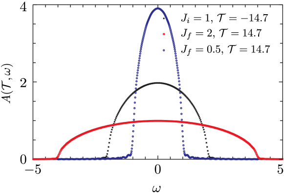
Figure 1: Spectral function of the random hopping model long before ($\mathcal{T}=-14.7$) and after ($\mathcal{T}=14.7$) a parameter quench from $J_{2,i}=1$ to $J_{2,f}=0.5$ and $2.0$.

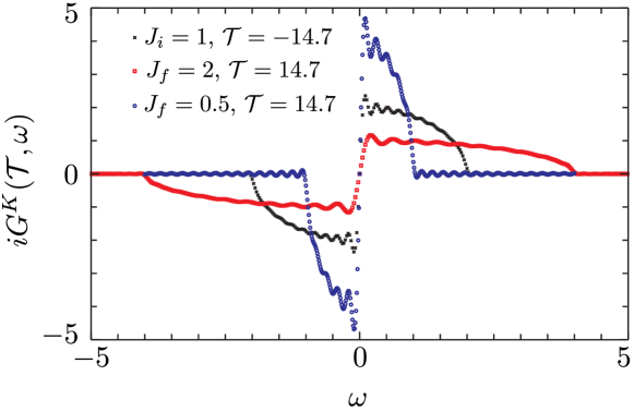
Figure 2: Keldysh component of the Green’s function of the random hopping model long before ($\mathcal{T}=-14.7$) and after ($\mathcal{T}=14.7$) a parameter quench from $J_{2,i}=1$ to $J_{2,f}=0.5$ and $2.0$.

Figure 1 shows the spectral function of the random hopping model long before and long after a parameter quench. These results were obtained from a numerical Fourier transformation of the retarded Green’s function as described by Eq. (48) with a broadening of $\delta=0.025$. In Fig. 2, we show the frequency dependence of the Keldysh component of the fermionic Green’s function for the same quench protocol as in Fig. 1.

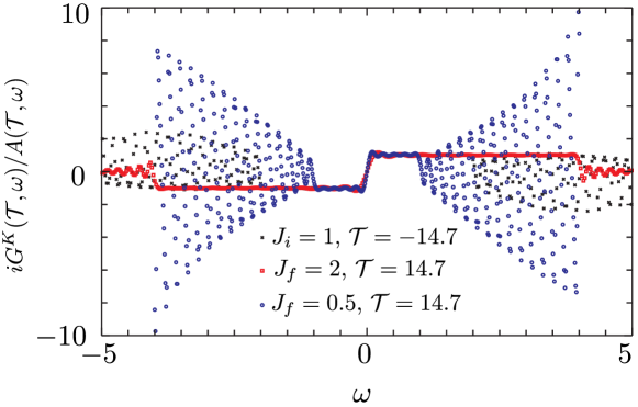
Figure 3: Ratio between the Keldysh component of the Green’s function and the spectral function of the random hopping model long before ($\mathcal{T}=-14.7$) and after ($\mathcal{T}=14.7$) a parameter quench from $J_{2,i}=1$ to $J_{2,f}=0.5$ and $2.0$.

In Fig. 3, we show the ratio between $iG^{K}(\mathcal{T},\omega)$ and $A(\mathcal{T},\omega)$ long before and after the parameter quench. The data is only reliable for frequencies $|\omega|<J_{2,f}$. For these frequencies, $iG^{K}(\mathcal{T},\omega)/A(\mathcal{T},\omega)$ is almost flat – up to numerical artifacts. We can determine the inverse temperature $\beta$ using Eq. (50), and find that $\beta J_{2}$ is roughly constant during the quench. All three results of this $(J_{2,i},0)\rightarrow(J_{2,f},0)$ quench are consistent with a rescaling of energy scales for all quantities. This is expected because the random hopping model has only one energy scale $J_{2}$, and the analog of the reparameterization in Eq. (54) applies here. For analytical expressions of the spectral functions we refer to Appendix A. We further comment, that whenever an energy scale appears to be one, we measure all other physical quantities with respect to this scale.

III.2 $(0,0)\rightarrow(0,J_{4})$ quench: From bare Majoranas to the SYK model

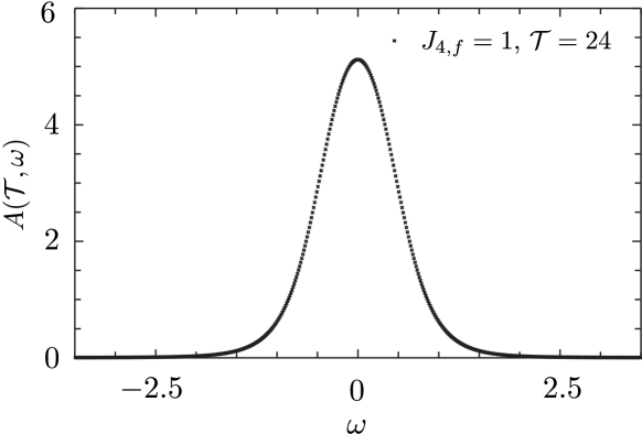
Figure 4: Spectral function of Majorana fermions long after suddenly switching on the quartic interaction of the SYK Hamiltonian, with $J_{4,f}=1$.

In Fig. 4, we show the spectral function long after suddely switching on the quartic interaction in the SYK model, starting from bare, noninteracting Majorana fermions. For an analytical expression of the thermal spectral function we refer to Appendix B. When interpreting results of this quench protocol, it is important to keep in mind that the Hamiltonian before the quench is zero, so that any finite $J_{4,f}$ is an arbitrarily strong perturbation.

In this scenario we find that the energy of the system does not change during the quench. It is zero before and after the quench, i. e. the quench did not pump energy into the system. The Keldysh component of the Green’s function vanishes before and after the quench. This is to be expected for free Majorana fermions and is consistent with the temperature of the system being infinite, i.e. $\beta_{f}=0$ after the quench.

We interpret this as a result of the particle-hole symmetry of the system before the quench when there is only one energy level at $\omega=0$. The quartic interaction broadens this energy level, but does not break the particle-hole symmetry. Thus, the spectral weight of the fermions is distributed over the entire spectrum. Alternatively, one can argue that the Hamiltonian before the quench is zero, so that any added interaction is in fact infinitely strong.

III.3 $(J_{2,i},0)\rightarrow(0,J_{4,f})$: From a quadratic to a quartic model

The quench from the purely quadratic to the purely quartic model decouples the regions $t_{1}(t_{2})<0$ from $t_{1}(t_{2})>0$ as can be seen by inspecting the structure of the Kadanoff-Baym equations and of the self-energy, which reads

$$\Sigma(t_{1},t_{2})=\Theta(-t_{1})\Theta(-t_{2})J_{2}^{2}G(t_{1},t_{2})-\Theta(t_{1})\Theta(t_{2})J_{4}^{2}G(t_{1},t_{2})^{3}$$ (51)

for this quench protocol. Inserting this into the Kadanoff-Baym equations for $t_{1}>0$ and $t_{2}>0$, one can see that all time integrals are restricted to positive times and the initial condition does not matter: Although $G^{>}(t_{1},t_{2})$ shows some time evolution for $t_{1}\gtrless 0$ and $t_{2}\lessgtr 0$ due to integrals involving the region with $t_{1}<0$ and $t_{2}<0$, $G^{>}$ in this region does not influence the time evolution at positive $t_{1}$, $t_{2}$ because $\Sigma(t_{1},t_{2})=0$ when $t_{1}\gtrless 0$ and $t_{2}\lessgtr 0$. Thus, the relevant initial condition for the time evolution of $G^{>}(t_{1},t_{2})$ is $iG^{>}(t_{1}=0,t_{2}=0)=1/2$. Hence propagating $iG^{>}$ forward in time using the self-energy of the quartic model, we obtain the same time evolution at positive times as when starting from bare Majorana fermions.

III.4 $(J_{2,i},J_{4,i})\rightarrow(0,J_{4,f})$ quench: $J_{2}$ + $J_{4}$ model to the SYK model

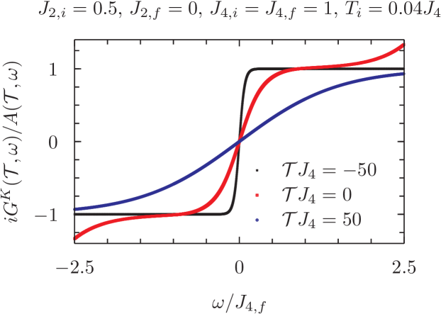
Figure 5: Numerical results of a quench from a $J_{2}$+$J_{4}$ model for $t<0$ to a purely $J_{4}$ model for $t>0$. Fits to this data allow determination of $\beta_{\text{eff}}(\mathcal{T})$.

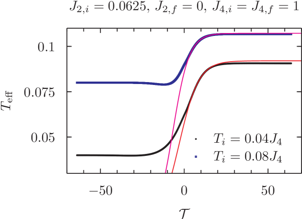
Figure 6: Fits to the values of $\beta_{\text{eff}}(\mathcal{T})=1/T_{\text{eff}}(\mathcal{T})$ from results like to those in Fig. 5 to Eq. (8) allow determination of $\Gamma$ for each quench.

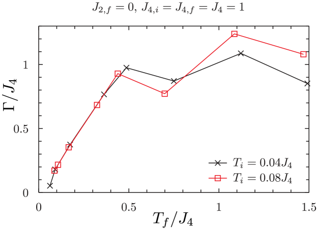
Figure 7: Plots of the values of $\Gamma$ obtained from Fig. 6 as a function of the final temperature of each quench. Note the proportionality of $\Gamma$ to $T_{f}$ at small $T_{f}$.

In this section, we discuss quenches from a Hamiltonian with a quadratic and a quartic term to a Hamiltonian, where the quadratic term is switched off. Particularly, the time scale of thermalization is the main interest. We study the validity of the flucutation-dissipation relation and the behavior of the effective temperature $T_{\text{eff}}(\mathcal{T})=\beta_{\text{eff}}^{-1}(\mathcal{T})$ in order to detect thermalization. The effective temperature can either be obtained from the derivative of $iG^{K}(\mathcal{T},\omega)/A(\mathcal{T},\omega)$ at $\omega=0$ or as fit of $\operatorname{tanh}[\omega/(2T_{\text{eff}})]$ to that function to some frequency interval. As shown in Fig. 5, long after the quench the numerical results for $iG^{K}(\mathcal{T},\omega)/A(\mathcal{T},\omega)$ are well described by $\operatorname{tanh}[\omega/(2T_{\text{eff}})]$, indicating that the system has thermalized. At intermediate times, the low frequency behaviour is still well described by this function. At high frequencies, deviations are visible which could arise due to the fact that $iG^{K}(\mathcal{T},\omega)/A(\mathcal{T},\omega)$ is non-thermal.

In Fig. 6 we show the time-dependence of the effective temperature and a fit of $T_{\text{eff}}^{-1}$ to Eq. (8). After the quench, the effective temperature shows exponential behavior. In Fig. 7 we show the thermalization rate as obtained from such fits. It appears proportional to the final temperature $T_{f}$ at small final temperatures as noted in Eq. (9), and saturates at higher temperatures. It is difficult to determine $\Gamma$ numerically at large $T_{f}/J_{4}$, and this likely leads to the oscillatory behavior present in Fig. 7.

IV Kadanoff-Baym equations: Large $q$ limit

This section will consider a model with a $q$ fermion coupling $J(t)$, and a $pq$ fermion coupling $J_{p}(t)$. For now, we keep the time-dependence of both couplings arbitrary. We will find that the initial state is exactly solvable for $p=2$ and $p=1/2$.

The Kadanoff-Baym equations in Eqs. (40), (41) and (42) for $G^{>}(t_{1},t_{2})$ now become

$$i\frac{\partial}{\partial t_{1}}G^{>}(t_{1},t_{2}) =-i^{q}\int_{-\infty}^{t_{1}}dt_{3}\,J(t_{1})J(t_{3})\left[(G^{>})^{q-1}(t_{1},t_{3})-(G^{<})^{q-1}(t_{1},t_{3})\right]G^{>}(t_{3},t_{2})$$

$$+i^{q}\int_{-\infty}^{t_{2}}dt_{3}\,J(t_{1})J(t_{3})(G^{>})^{q-1}(t_{1},t_{3})\left[G^{>}(t_{3},t_{2})-G^{<}(t_{3},t_{2})\right]$$

$$-i^{pq}\int_{-\infty}^{t_{1}}dt_{3}\,J_{p}(t_{1})J_{p}(t_{3})\left[(G^{>})^{pq-1}(t_{1},t_{3})-(G^{<})^{pq-1}(t_{1},t_{3})\right]G^{>}(t_{3},t_{2})$$

$$+i^{pq}\int_{-\infty}^{t_{2}}dt_{3}\,J_{p}(t_{1})J_{p}(t_{3})(G^{>})^{pq-1}(t_{1},t_{3})\left[G^{>}(t_{3},t_{2})-G^{<}(t_{3},t_{2})\right]\,,$$

$$-i\frac{\partial}{\partial t_{2}}G^{>}(t_{1},t_{2}) =-i^{q}\int_{-\infty}^{t_{1}}dt_{3}\,J(t_{3})J(t_{2})\left[G^{>}(t_{1},t_{3})-G^{<}(t_{1},t_{3})\right](G^{>})^{q-1}(t_{3},t_{2})$$

$$+i^{q}\int_{-\infty}^{t_{2}}dt_{3}\,J(t_{3})J(t_{2})G^{>}(t_{1},t_{3})\left[(G^{>})^{q-1}(t_{3},t_{2})-(G^{<})^{q-1}(t_{3},t_{2})\right]$$

$$-i^{pq}\int_{-\infty}^{t_{1}}dt_{3}\,J_{p}(t_{3})J_{p}(t_{2})\left[G^{>}(t_{1},t_{3})-G^{<}(t_{1},t_{3})\right](G^{>})^{pq-1}(t_{3},t_{2})$$ (52)

$$+i^{pq}\int_{-\infty}^{t_{2}}dt_{3}\,J_{p}(t_{3})J_{p}(t_{2})G^{>}(t_{1},t_{3})\left[(G^{>})^{pq-1}(t_{3},t_{2})-(G^{<})^{pq-1}(t_{3},t_{2})\right]\,.$$

where we have defined

$$J_{p}(t)\equiv J_{p}f(t)\quad,\quad J(t)\equiv Jf(t)\,.$$ (53)

Also, recall that Eq. (31) relates $G^{>}$ to $G^{<}$.

We note a property of the Kadanoff-Baym equations in Eq. (52), connected to a comment in Section I above Eq. (6). If we set $J_{p}(t)=0$, then all dependence of Eq. (52) on $J(t)$ can be scaled away by reparameterizing time via

$$\int^{t}J(t^{\prime})dt^{\prime}\rightarrow t\,.$$ (54)

This implies that correlations remain in thermal equilibrium in the new time co-ordinate. However, when both $J_{p}(t)$ and $J(t)$ are non-zero, such a reparameterization is not sufficient, and there is non-trivial quench dynamics, as was shown by our numerical study in Section III. Below, we will see that the quench dynamics can also be trivial in the limit $q\rightarrow\infty$, even when both $J_{p}(t)$ and $J(t)$ are both non-zero. But this result arises from fairly non-trivial computations which are described below, and in particular from an SL(2,C) symmetry of the parameterization of the equations.

In the large $q$ limit, we assume a solution of the form in Eq. (10). Inserting (10) into (52), we obtain to leading order in $1/q$

$$\frac{\partial}{\partial t_{1}}g(t_{1},t_{2}) = 2\int_{-\infty}^{t_{2}}dt_{3}\,\mathcal{J}(t_{1})\mathcal{J}(t_{3})e^{g(t_{1},t_{3})}-\int_{-\infty}^{t_{1}}dt_{3}\,\mathcal{J}(t_{1})\mathcal{J}(t_{3})\left[e^{g(t_{1},t_{3})}+e^{g(t_{3},t_{1})}\right]$$

$$+ 2\int_{-\infty}^{t_{2}}dt_{3}\,\mathcal{J}_{p}(t_{1})\mathcal{J}_{p}(t_{3})e^{pg(t_{1},t_{3})}-\int_{-\infty}^{t_{1}}dt_{3}\,\mathcal{J}_{p}(t_{1})\mathcal{J}_{p}(t_{3})\left[e^{pg(t_{1},t_{3})}+e^{pg(t_{3},t_{1})}\right]\,,$$

$$\frac{\partial}{\partial t_{2}}g(t_{1},t_{2}) = 2\int_{-\infty}^{t_{1}}dt_{3}\,\mathcal{J}(t_{3})\mathcal{J}(t_{2})e^{g(t_{3},t_{2})}-\int_{-\infty}^{t_{2}}dt_{3}\,\mathcal{J}(t_{3})\mathcal{J}(t_{2})\left[e^{g(t_{3},t_{2})}+e^{g(t_{2},t_{3})}\right]$$

$$+ 2\int_{-\infty}^{t_{1}}dt_{3}\,\mathcal{J}_{p}(t_{3})\mathcal{J}_{p}(t_{2})e^{pg(t_{3},t_{2})}-\int_{-\infty}^{t_{2}}dt_{3}\,\mathcal{J}_{p}(t_{3})\mathcal{J}_{p}(t_{2})\left[e^{pg(t_{3},t_{2})}+e^{pg(t_{2},t_{3})}\right]\,,$$

where

$$\mathcal{J}^{2}(t)=qJ^{2}(t)2^{1-q}\quad,\quad\mathcal{J}_{p}^{2}(t)=qJ_{p}^{2}(t)2^{1-pq}$$ (56)

It is a remarkable fact that these non-linear, partial, integro-differential equations are exactly solvable for our quench protocol and all initial conditions, as we will show in the remainder of this section. The final exact solution appears in Section IV.4, and surprisingly shows that the solution is instantaneously in thermal equilibrium at $t=0^{+}$.

Taking the derivatives of either equation in Eq. (IV) we obtain

$$\frac{\partial^{2}}{\partial t_{1}\partial t_{2}}g(t_{1},t_{2})=2\mathcal{J}(t_{1})\mathcal{J}(t_{2})e^{g(t_{1},t_{2})}+2\mathcal{J}_{p}(t_{1})\mathcal{J}_{p}(t_{2})e^{pg(t_{1},t_{2})}\,.$$ (57)

We will look at the case where $\mathcal{J}_{p}(t)$ is non-zero only for $t<0$, while $\mathcal{J}(t)$ is time independent:

$$\mathcal{J}_{p}(t)=\mathcal{J}_{p}\,\Theta(-t)\quad,\quad\mathcal{J}(t)=\mathcal{J}\,.$$ (58)

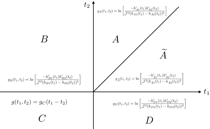
Figure 8: The regions in the $t_{1}$-$t_{2}$ plane.

Then Eq. (57) is the Lorentzian Liouville equation in three of the four quadrants of the $t_{1}$-$t_{2}$ plane (labeled as in Fig. 8), and its most general solution in these quadrants is

$$g_{\alpha}(t_{1},t_{2})=\ln\left[\frac{-h_{\alpha 1}^{\prime}(t_{1})h_{\alpha 2}^{\prime}(t_{2})}{\mathcal{J}^{2}(h_{\alpha 1}(t_{1})-h_{\alpha 2}(t_{2}))^{2}}\right]\quad,\quad\mbox{for $\alpha=A,\widetilde{A},B,D$}\,.$$ (59)

Eq. (59) will also apply for $\alpha=C$ when $\mathcal{J}_{p}=0$. Eq. (11) implies that the functions $h_{A1}(t)$ and $h_{A2}(t)$ obey

$$h_{A1}^{\prime}(t)h_{A2}^{\prime}(t)=-\mathcal{J}^{2}(h_{A1}(t)-h_{A2}(t))^{2}\,,$$ (60)

and similarly

$$h_{\widetilde{A}1}^{\prime}(t)h_{\widetilde{A}2}^{\prime}(t)=-\mathcal{J}^{2}(h_{\widetilde{A}1}(t)-h_{\widetilde{A}2}(t))^{2}\,,$$ (61)

Note that $g_{\alpha}(t_{1},t_{2})$ remains invariant under the SL(2,C) mapping in Eq. (14). Given the symmetries of Eq. (IV) and the thermal initial conditions, we look for solutions which obey

$$g(t_{2},t_{1})=\left[g(t_{1},t_{2})\right]^{\ast}\,.$$ (62)

This property can be related to the causality of the Kadanoff-Baym equations as is explained in Appendix D. We can satisfy Eq. (62) in quadrants A, B, D by the relations

$$h_{\widetilde{A}1}(t) = h_{A2}^{\ast}(t)\,,$$

$$h_{\widetilde{A}2}(t) = h_{A1}^{\ast}(t)\,,$$

$$h_{D1}(t) = h_{B2}^{\ast}(t)\,,$$

$$h_{D2}(t) = h_{B1}^{\ast}(t)\,.$$ (63)

The system is in equilibrium in quadrant C, and so the Green’s function depends only upon time differences. We describe the nature of this equilibrium solution in Appendix E. In the following subsections, we describe the results of inserting the parameterization in Eq. (59) back into Eq. (IV) to obtain ordinary differential equations for $h_{\alpha 1}$ and $h_{\alpha 2}$.

IV.1 Quadrant B

From Eq. (IV), we obtain for $t_{1}<0$ and $t_{2}>0$

$$-\frac{\partial}{\partial t_{1}}g_{B}(t_{1},t_{2}) = -\mathcal{J}^{2}\int_{-\infty}^{\infty}dt^{\prime}\,e^{g_{C}(t^{\prime})}\,\mbox{sgn}(t^{\prime}-t_{1})-2\mathcal{J}^{2}\int_{0}^{t_{2}}dt_{3}\,e^{g_{B}(t_{1},t_{3})}$$

$$~{}~{}~{}~{}~{}-\mathcal{J}_{p}^{2}\int_{-\infty}^{\infty}dt^{\prime}\mbox{sgn}(t^{\prime}-t_{1})e^{pg_{C}(t^{\prime})}\,,$$

$$\frac{\partial}{\partial t_{2}}g_{B}(t_{1},t_{2}) = 2\mathcal{J}^{2}\int_{-\infty}^{t_{1}}dt_{3}\,e^{g_{B}(t_{3},t_{2})}-\mathcal{J}^{2}\int_{-\infty}^{0}dt_{3}\,\left[e^{g_{B}(t_{3},t_{2})}+e^{g_{D}(t_{2},t_{3})}\right]$$ (64)

$$~{}~{}~{}~{}~{}-\mathcal{J}^{2}\int_{0}^{t_{2}}dt_{3}\,\left[e^{g_{A}(t_{3},t_{2})}+e^{g_{\widetilde{A}}(t_{2},t_{3})}\right]\,.$$

Inserting Eq. (59) in Eq. (64) we obtain

$$-\frac{h_{B1}^{\prime\prime}(t_{1})}{h_{B1}^{\prime}(t_{1})} = -\mathcal{J}^{2}\int_{-\infty}^{\infty}dt^{\prime}\,e^{g_{C}(t^{\prime})}\,\mbox{sgn}(t^{\prime}-t_{1})-\frac{2h_{B1}^{\prime}(t_{1})}{h_{B1}(t_{1})-h_{B2}(0)}$$ (65)

$$~{}~{}~{}~{}~{}-\mathcal{J}_{p}^{2}\int_{-\infty}^{\infty}dt^{\prime}\mbox{sgn}(t^{\prime}-t_{1})e^{pg_{C}(t^{\prime})}\,,$$

$$\frac{h_{B2}^{\prime\prime}(t_{2})}{h_{B2}^{\prime}(t_{2})} = -\frac{2h_{B2}^{\prime}(t_{2})}{h_{B1}(-\infty)-h_{B2}(t_{2})}$$

$$-\frac{h_{B2}^{\prime}(t_{2})}{h_{B1}(0)-h_{B2}(t_{2})}+\frac{h_{B2}^{\prime}(t_{2})}{h_{B1}(-\infty)-h_{B2}(t_{2})}-\frac{h_{B2}^{\ast\prime}(t_{2})}{h_{B1}^{\ast}(0)-h_{B2}^{\ast}(t_{2})}+\frac{h_{B2}^{\ast\prime}(t_{2})}{h_{B1}^{\ast}(-\infty)-h_{B2}^{\ast}(t_{2})}$$

$$-\frac{h_{A2}^{\prime}(t_{2})}{h_{A1}(t_{2})-h_{A2}(t_{2})}+\frac{h_{A2}^{\prime}(t_{2})}{h_{A1}(0)-h_{A2}(t_{2})}-\frac{h_{A2}^{\ast\prime}(t_{2})}{h_{A1}^{\ast}(t_{2})-h_{A2}^{\ast}(t_{2})}+\frac{h_{A2}^{\ast\prime}(t_{2})}{h_{A1}^{\ast}(0)-h_{A2}^{\ast}(t_{2})}\,.$$

We also have the compatibility condition at the boundary between regions B and C, which is

$$g_{C}(t_{1})=\ln\left[\frac{-h_{B1}^{\prime}(t_{1})h_{B2}^{\prime}(0)}{\mathcal{J}^{2}(h_{B1}(t_{1})-h_{B2}(0))^{2}}\right]\,;$$ (67)

taking the derivative of this equation we obtain precisely the first equation in Eq. (65) after using Eq. (109). This reassures us that the system of equations are not overdetermined. We can easily integrate Eq. (67) to obtain

$$\frac{h_{B2}^{\prime}(0)}{h_{B1}(t_{1})-h_{B2}(0)}-\frac{h_{B2}^{\prime}(0)}{h_{B1}(-\infty)-h_{B2}(0)}=\mathcal{J}^{2}\int_{-\infty}^{t_{1}}dt\,e^{g_{C}(t)}\,.$$ (68)

IV.2 Region A

Now $t_{2}>t_{1}>0$. From the second Eq. (IV) we obtain

$$\frac{\partial}{\partial t_{2}}g_{A}(t_{1},t_{2}) = 2\mathcal{J}^{2}\int_{-\infty}^{0}dt_{3}\,e^{g_{B}(t_{3},t_{2})}+2\mathcal{J}^{2}\int_{0}^{t_{1}}dt_{3}\,e^{g_{A}(t_{3},t_{2})}-\mathcal{J}^{2}\int_{-\infty}^{0}dt_{3}\,\left[e^{g_{B}(t_{3},t_{2})}+e^{g_{D}(t_{2},t_{3})}\right]$$ (69)

$$~{}~{}~{}~{}~{}-\mathcal{J}^{2}\int_{0}^{t_{2}}dt_{3}\,\left[e^{g_{A}(t_{3},t_{2})}+e^{g_{\widetilde{A}}(t_{2},t_{3})}\right]\,.$$

Inserting Eq. (59) into Eq. (69), we obtain

$$\frac{h_{A2}^{\prime\prime}(t_{2})}{h_{A2}^{\prime}(t_{2})} = \frac{2h_{B2}^{\prime}(t_{2})}{h_{B1}(0)-h_{B2}(t_{2})}-\frac{2h_{B2}^{\prime}(t_{2})}{h_{B1}(-\infty)-h_{B2}(t_{2})}-\frac{2h_{A2}^{\prime}(t_{2})}{h_{A1}(0)-h_{A2}(t_{2})}$$

$$-\frac{h_{B2}^{\prime}(t_{2})}{h_{B1}(0)-h_{B2}(t_{2})}+\frac{h_{B2}^{\prime}(t_{2})}{h_{B1}(-\infty)-h_{B2}(t_{2})}-\frac{h_{B2}^{\ast\prime}(t_{2})}{h_{B1}^{\ast}(0)-h_{B2}^{\ast}(t_{2})}+\frac{h_{B2}^{\ast\prime}(t_{2})}{h_{B1}^{\ast}(-\infty)-h_{B2}^{\ast}(t_{2})}$$

$$-\frac{h_{A2}^{\prime}(t_{2})}{h_{A1}(t_{2})-h_{A2}(t_{2})}+\frac{h_{A2}^{\prime}(t_{2})}{h_{A1}(0)-h_{A2}(t_{2})}-\frac{h_{A2}^{\ast\prime}(t_{2})}{h_{A1}^{\ast}(t_{2})-h_{A2}^{\ast}(t_{2})}+\frac{h_{A2}^{\ast\prime}(t_{2})}{h_{A1}^{\ast}(0)-h_{A2}^{\ast}(t_{2})}\,.$$

From the first Eq. (IV) we obtain

$$-\frac{\partial}{\partial t_{1}}g_{A}(t_{1},t_{2}) = -\mathcal{J}^{2}\int_{-\infty}^{0}dt_{3}\,e^{g_{D}(t_{1},t_{3})}-\mathcal{J}^{2}\int_{0}^{t_{1}}dt_{3}\,e^{g_{\widetilde{A}}(t_{1},t_{3})}-2\mathcal{J}^{2}\int_{t_{1}}^{t_{2}}dt_{3}\,e^{g_{A}(t_{1},t_{3})}$$ (71)

$$~{}+\mathcal{J}^{2}\int_{-\infty}^{0}dt_{3}\,e^{g_{B}(t_{3},t_{1})}+\mathcal{J}^{2}\int_{0}^{t_{1}}dt_{3}\,e^{g_{A}(t_{3},t_{1})}\,.$$

Inserting Eq. (59) into Eq. (71), we obtain

$$-\frac{h_{A1}^{\prime\prime}(t_{1})}{h_{A1}^{\prime}(t_{1})} = \frac{2h_{A1}^{\prime}(t_{1})}{h_{A2}(t_{1})-h_{A1}(t_{1})}$$

$$~{}-\frac{h_{B2}^{\ast\prime}(t_{1})}{h_{B1}^{\ast}(0)-h_{B2}^{\ast}(t_{1})}+\frac{h_{B2}^{\ast\prime}(t_{1})}{h_{B1}^{\ast}(-\infty)-h_{B2}^{\ast}(t_{1})}+\frac{h_{B2}^{\prime}(t_{1})}{h_{B1}(0)-h_{B2}(t_{1})}-\frac{h_{B2}^{\prime}(t_{1})}{h_{B1}(-\infty)-h_{B2}(t_{1})}$$

$$~{}+\frac{h_{A2}^{\prime}(t_{1})}{h_{A1}(t_{1})-h_{A2}(t_{1})}-\frac{h_{A2}^{\prime}(t_{1})}{h_{A1}(0)-h_{A2}(t_{1})}-\frac{h_{A2}^{\ast\prime}(t_{1})}{h_{A1}^{\ast}(t_{1})-h_{A2}^{\ast}(t_{1})}+\frac{h_{A2}^{\ast\prime}(t_{1})}{h_{A1}^{\ast}(0)-h_{A2}^{\ast}(t_{1})}\,.$$

From Eqs. (IV.2) and (IV.2) we obtain

$$\frac{h_{A1}^{\prime\prime}(t)}{h_{A1}^{\prime}(t)}+\frac{h_{A2}^{\prime\prime}(t)}{h_{A2}^{\prime}(t)}=2\left(\frac{h_{A1}^{\prime}(t)-h_{A2}^{\prime}(t)}{h_{A1}(t)-h_{A2}(t)}\right)\,.$$ (73)

This is precisely the logarithmic derivative of the Majorana condition in Eq. (60). The compatibility condition at the boundary of region A and region B is

$$\frac{h_{A1}^{\prime}(0)h_{A2}^{\prime}(t_{2})}{(h_{A1}(0)-h_{A2}(t_{2}))^{2}}=\frac{h_{B1}^{\prime}(0)h_{B2}^{\prime}(t_{2})}{(h_{B1}(0)-h_{B2}(t_{2}))^{2}}\,.$$ (74)

This can be integrated to

$$\frac{h_{A1}^{\prime}(0)}{h_{A2}(t_{2})-h_{A1}(0)}=\frac{h_{B1}^{\prime}(0)}{h_{B2}(t_{2})-h_{B1}(0)}+c_{4}\,,$$ (75)

where $c_{4}$ is a constant of integration.

IV.3 Combined equations

We adopt a simple choice to solve Eq. (75)

$$h_{B2}(t) = h_{A2}(t)\,,$$

$$h_{B1}(0) = h_{A1}(0)\,,$$

$$h_{B1}^{\prime}(0) = h_{A1}^{\prime}(0)\,.$$ (76)

Then we find that Eqs. (IV.1) and (IV.2) are consistent with each other. Collecting all equations, we need to solve

$$-\frac{h_{A1}^{\prime\prime}(t)}{h_{A1}^{\prime}(t)} =-\frac{2h_{A1}^{\prime}(t)}{h_{A1}(t)-h_{A2}(t)}+\frac{h_{A2}^{\ast\prime}(t)}{h_{B1}^{\ast}(-\infty)-h_{A2}^{\ast}(t)}-\frac{h_{A2}^{\prime}(t)}{h_{B1}(-\infty)-h_{A2}(t)}$$

$$+\frac{h_{A2}^{\prime}(t)}{h_{A1}(t)-h_{A2}(t)}-\frac{h_{A2}^{\ast\prime}(t)}{h_{A1}^{\ast}(t)-h_{A2}^{\ast}(t)}\quad,\quad t\geq 0$$ (77)

$$h_{A1}^{\prime}(t)h_{A2}^{\prime}(t) =-\mathcal{J}^{2}(h_{A1}(t)-h_{A2}(t))^{2}\quad,\quad t\geq 0$$ (78)

$$\frac{h_{B2}^{\prime}(0)}{h_{B1}(t)-h_{B2}(0)} =\frac{h_{B2}^{\prime}(0)}{h_{B1}(-\infty)-h_{B2}(0)}+\mathcal{J}^{2}\int_{-\infty}^{t}dt^{\prime}\,e^{g_{C}(t^{\prime})}\quad,\quad t\leq 0$$ (79)

$$h_{A1}(0) =h_{B1}(0)\,,$$ (80)

$$h_{A1}^{\prime}(0) =h_{B1}^{\prime}(0)\,,$$ (81)

$$h_{A2}(0) =h_{B2}(0)\,.$$ (82)

It can be verified that all expressions above are invariant SL(2,C) transformations of the $h_{\alpha 1}$ and $h_{\alpha 2}$ fields. Given the values of $h_{B1}(-\infty)$, $h_{B2}(0)$, $h_{B2}^{\prime}(0)$, and $g_{C}(t)$, Eqs. (79-82) determine the values of $h_{A1}(0)$, $h_{A1}^{\prime}(0)$, and $h_{A2}(0)$. Then Eqs. (77,78) uniquely determine $h_{A1}(t)$ and $h_{A2}(t)$ for all $t\geq 0$. Because of the SL(2,C) invariance, the values chosen for $h_{B1}(-\infty)$, $h_{B2}(0)$, $h_{B2}^{\prime}(0)$ won’t matter for the final result for $g_{A}(t_{1},t_{2})$.

IV.4 Exact solution

A solution of the form in Eq. (123) does not apply to Eqs. (77-82) in region A because it does not have enough free parameters to satisfy the initial conditions. However, we can use the SL(2,C) invariance of Eqs. (77-79) to propose the ansatz similar to that in Eq. (15) (here, we redefine constants by factors of $e^{i\theta}$):

$$h_{A1}(t)=\frac{a\,e^{\sigma t}+c}{c\,e^{\sigma t}+d}\quad,\quad h_{A2}(t)=\frac{a\,e^{-2i\theta}e^{\sigma t}+b}{c\,e^{-2i\theta}e^{\sigma t}+d}\,.$$ (83)

We can now verify that Eq. (83) is an exact solution of Eqs. (77-82). This solution is characterized by 4 complex numbers $a$, $b$, $c$, $d$ and two real numbers $\theta$, $\sigma$. These are uniquely determined from the values of $h_{B1}(-\infty)$, $h_{A1}(0)$, $h_{A1}^{\prime}(0)$, and $h_{A2}(0)$ by the solution of the following 6 equations

$$ad-bc =1\,,$$

$$\sigma =2\mathcal{J}\sin(\theta)\,,$$

$$e^{-4i\theta} =\frac{(b-d\,h_{B1}(-\infty))(a^{\ast}-c^{\ast}\,h_{B1}^{\ast}(-\infty))}{(b^{\ast}-d^{\ast}\,h_{B1}^{\ast}(-\infty))(a-c\,h_{B1}(-\infty))}\,,$$

$$h_{A1}(0) =\frac{a+b}{c+d}\,,$$

$$h_{A2}(0) =\frac{a\,e^{-2i\theta}+b}{c\,e^{-2i\theta}+d}\,,$$

$$h_{A1}^{\prime}(0) =\frac{2\sin(\theta)}{(c+d)^{2}}\,.$$ (84)

It is now easy to verify that $g_{A}$ takes the form in Eq. (17), and so all of quadrant A is also in thermal equilibrium. We also numerically integrated Eqs. (77-82), starting from generic initial conditions, and verified that the numerical solution obeyed the expressions in Eqs. (83) and (84).

The above solution determines the values of $\sigma$ and $\theta$ in the final state, and hence the value of the final temperature via Eq. (18). In general, this will be different from the value of the initial temperature in quadrant C.

Eqs. (83) and (84) also determine the solutions in the other quadrants via expressions specified earlier. The solutions in region $\widetilde{A}$ follow from the conjugacy property in Eq. (63). In quadrant B, we have $h_{B2}(t)=h_{A2}(t)$ in Eq. (76), while $h_{B1}(t)$ was specified in Eq. (68) using the initial state in quadrant C. Note that the solution in quadrant B is not of a thermal form, as $h_{B1}$ and $h_{B2}$ are not simply related as in Eq. (83). The solution in quadrant D follows from that in quadrant B via the conjugacy property in Eq. (63). And, finally, the initial state in quadrant C was described in Appendix E.

V Conclusions

Quantum many-body systems without quasiparticle excitations are expected to locally thermalize in the fastest possible times of order $\hbar/(k_{B}T)$ as $T\rightarrow 0$, where $T$ is the absolute temperature of the final state Sachdev (1999). This excludes e.g. the existence of systems in which the local thermalization rate, $\Gamma\sim T^{p}$ as $T\rightarrow 0$ with $p<1$, and no counterexamples have been found.

In this paper we examined SYK models, which are systems which saturate the more rigorous bounds on the Lyapunov time to reach quantum chaos Maldacena et al. (2016). Our numerical study of the model with a final Hamiltonian with $q=4$ showed that this system does thermalize rapidly, and the thermalization rate is consistent with $\Gamma=CT$ at low $T$ where $C$ is dimensionless constant, as indicated in Eq. (9) and Fig. 7.

We also studied a large $q$ limit of the SYK models, where an exact analytic solution of the non-equilibrium dynamics was possible. Here we found that thermalization of the fermion Green’s function was instantaneous. It will be necessary to study higher order corrections in $1/q$ to understand how this connects to the numerical $q=4$ numerical solution: does the constant $C\rightarrow\infty$ as $q\rightarrow\infty$, or (as pointed to us by Aavishkar Patel) is thermalization at large $q$ a two-step process. In two-step scenario, a very rapid pre-thermalization (which we have computed) is followed by a slower true thermalization of higher order corrections.

Finally, we comment on a remarkable feature of the large $q$ solution given by Eq. (13) and (15): its connection with the Schwarzian. The Schwarzian was proposed as an effective Lagrangian for the low energy limit of the equilibrium theory. Specifically, consider the Euler-Lagrange equation of motion of a Lagrangian, $\mathcal{L}$, which is the Schwarzian of $h(t)$

$$\mathcal{L}[h(t)]=\frac{h^{\prime\prime\prime}(t)}{h^{\prime}(t)}-\frac{3}{2}\left(\frac{h^{\prime\prime}(t)}{h^{\prime}(t)}\right)^{2}\,.$$ (85)

The equation of motion is

$$\left[h^{\prime}(t)\right]^{2}h^{\prime\prime\prime\prime}(t)+3\left[h^{\prime\prime}(t)\right]^{3}-4h^{\prime}(t)h^{\prime\prime}(t)h^{\prime\prime\prime}(t)=0\,.$$ (86)

It can now be verified that the expressions for $h_{1,2}(t)$ in Eq. (15) (and Eq. (83)) both obey Eq. (86). We note, however, that we did not obtain Eq. (15) by the solution of Eq. (86): instead, Eq. (15) was obtained by the solution of the Schwinger-Keldysh equations of the large-$q$ SYK model in Eq. (IV). This connection with the Schwarzian indicates that gravitational models Sachdev (2010a, b); Almheiri and Polchinski (2015); Kitaev (2015); Maldacena and Stanford (2016); Jensen (2016); Engelsöy et al. (2016) of the quantum quench in AdS₂, which map to a Schwarzian boundary theory, exhibit instant thermalization as in the large $q$ limit.

Indeed, the equation of motion of the metric in two-dimensional gravity Almheiri and Polchinski (2015) takes a form identical to that for the two-point fermion correlator in Eq. (12). And studies of black hole formation in AdS₂ from a collapsing shell of matter show that the Hawking temperature of the black hole jumps instantaneously to a new equilibrium value after the passage of the shell Engelsöy et al. (2016); Engelsöy (2017). These features are strikingly similar to those obtained in our large $q$ analysis. There have been studies of quantum quenches in AdS₂, either in the context of quantum impurity problems Erdmenger et al. (2017), or in the context of higher-dimensional black holes which have an AdS₂ factor in the low energy limit Withers (2016); it would be useful to analytically extract the behavior of just AdS₂ by extending such studies.

We thank J. Maldacena of informing us about another work Kourkoulou and Maldacena (2017) which studied aspects of thermalization of SYK models by very different methods, along with connections to gravity on AdS₂.

Appendix A Spectral function and Green’s functions of random hopping model

The random hopping model of Majorana fermions, i. e.the SYK Hamiltonian for $q=2$, can be solved exactly Maldacena and Stanford (2016). We repeat the calculation within our notation in the following. The Matsubara Green’s function follows from the solution of

$$G(i\omega_{n})^{-1}=i\omega_{n}-\Sigma(i\omega_{n})=i\omega_{n}+J_{2}^{2}G(i\omega_{n}).$$ (87)

This can be rewritten as a quadratic equation for $\bigl{(}G(i\omega_{n})\bigr{)}^{-1}$ and matching the branches with the correct high-frequency asymptotics and symmetry yields the propagator

$$G(i\omega_{n})=\frac{2}{i\omega_{n}+i\operatorname{sgn}(\omega_{n})\sqrt{\omega_{n}^{2}+4J_{2}^{2}}}.$$ (88)

Analytically continuing to the real frequency axis from the upper half plane yields the retarded Green’s function,

$$G^{R}(\omega+i\delta)=\frac{2}{\omega+i\delta+i\sqrt{4J_{2}^{2}-(\omega+i\delta)^{2}}},$$ (89)

where $\delta$ can be set to zero due to the presence of the finite imaginary part. Note that we exploited that $\operatorname{sgn}\omega_{n}\rightarrow 1$ in the analytic continuation from the upper half plane. We obtain

$$A(\omega)=-2\operatorname{Im}G^{R}(\omega+i\delta)=\frac{2}{J_{2}}\sqrt{1-\Bigl{(}\frac{\omega}{2J_{2}}\Bigr{)}^{2}}\qquad\text{for }|\omega|<2J_{2},$$ (90)

which is the well-known semicircular density of states due to random hopping.

This yields

$$iG^{>}(t)=\frac{1}{2J_{2}t}\bigl{(}J_{1}(2J_{2}t)-iH_{1}(2J_{2}t)\bigr{)},$$ (91)

where $J_{1}$ and $H_{1}$ are the Bessel function of the first kind (BesselJ in Mathematica) and the Struve function (StruveH in Mathematica), respectively.

Appendix B Spectral Function in the Conformal Limit

In the scaling limit at non-zero temperature the retarded Green’s function is given by the following expression

$$iG^{R}(t)=2b(\cos\pi\Delta)\left(\frac{\pi}{\beta\sinh\frac{\pi t}{\beta}}\right)^{2\Delta}\theta(t)\,,$$ (92)

where $\Delta=1/q$ is the fermion scaling dimension. At $q=4$ we obtain

$$iG^{R}_{c}(t)=\sqrt{2}b\left(\frac{\pi}{\beta\sinh\frac{\pi t}{\beta}}\right)^{\frac{1}{2}}\theta(t)$$ (93)

The Wigner transform of the retarded Green’s functions is given by

$$iG^{R}(\omega) =\sqrt{2}b\int_{0}^{\infty}dte^{i\omega t}\left(\frac{\pi}{\beta\sinh\frac{\pi t}{\beta}}\right)^{\frac{1}{2}}$$

$$=b\left(\frac{\pi}{\beta}\right)^{-\frac{1}{2}}B\left(\frac{1}{2};\frac{1}{4}-\frac{i\beta\omega}{2\pi}\right)\,,$$ (94)

where $b=({4\pi J^{2}_{4}})^{-{1}/{4}}$. The associated spectral function is

$$A(\mathcal{T},\omega)=2b\left(\frac{\pi}{\beta}\right)^{-\frac{1}{2}}\text{Re}\left[B\left(\frac{1}{2};\frac{1}{4}-\frac{i\beta\omega}{2\pi}\right)\right]\,.$$ (95)

Appendix C Details on the Numerical Solution of Kadanoff-Baym equation

The Green’s function is typically determined on two-dimensional grids in $(t,t^{\prime})$ space with $8000\times 8000$ or $12000\times 12000$ points, where the quench happens after half of the points in each direction. When starting from initial states in which only $J_{2}$ is finite, the Green’s function decays algebraically in time. This leads to significant finite size effects in Fourier transforms. In order to reduce the latter, most numerical results were obtained by starting from a thermal state in which $J_{2}$ and $J_{4}$, or only $J_{4}$, are finite. In these cases, the Green’s function decays exponentially as a function of the relative time dependence.

We checked the quality and consistency of the results by monitoring the conservation of energy, the normalization of the spectral function and the real and imaginary part of the retarded propagator are Kramers-Kronig consistent for long times after the quench.

In order to time-evolve the Kadanoff-Baym equations we have to determine $G^{<}(t_{1},t_{2})$ for $t_{1},t_{2}$. When quenching the ground state of the random hopping model, we can use the exact solution for $G^{>}$ as initial condition. When we do not have an analytical expression the Green’s function we solve the Dyson equation self-consistently according to the following scheme:

1. Prepare $iG^{>}$ with an initial guess, for example the propagator of the random hopping model.

2. Computation of retarded self-energy in time domain:

   $$i\Sigma^{R}(t)=\Theta(t)(i\Sigma^{>}(t)+i\Sigma^{>}(-t))$$ (96)

3. Fourier transformation

   $$i\Sigma^{R}(\omega)=\int_{-\infty}^{\infty}dte^{i\omega t}i\Sigma^{R}(t)$$ (97)

4. Dyson equation:

   $$G^{R}(\omega)=\frac{1}{\omega-\Sigma^{R}(\omega)}$$ (98)

5. Determine spectral function

   $$A(\omega)=-2\operatorname{Im}G^{R}(\omega)$$ (99)

6. Determine $iG^{>}(\omega)$ from spectral function,

   $$iG^{>}(\omega)=(1-n_{F}(\omega))A(\omega)$$ (100)

   Note that this is the only step in the self-consistency procedure where the temperature $\beta^{-1}$ enters through the Fermi function $n_{F}$.

7. Fourier transformation to time domain

   $$iG^{>}(t)=\int_{-\infty}^{\infty}\frac{d\omega}{2\pi}e^{-i\omega t}iG^{>}(\omega)$$ (101)

8. Continue with step 2 until convergence is reached.

Appendix D Conjugacy property of $g(t_{1},t_{2})$

In this appendix we illustrate that the causality structure of the Kadanoff-Baym equations eq. (IV) leads to the property

$$[g(t_{1},t_{2})]^{\ast}=g(t_{2},t_{1})$$ (102)

in all four quadrants of Fig. 9. Since the system is thermal in quadrant $C$ the conjugacy property $[g(t_{1},t_{2})]^{\ast}=g(t_{2},t_{1})$ can be read off the thermal solution for $t_{1},t_{2}\leq 0$. Next, we consider the propagation from the line $\left\{(t_{1},t_{2})\in\mathbb{R}^{2}\,|t_{2}=0,t_{1}\leq 0\right\}$ for an infinitesimal time $\Delta t$ in the $t_{2}$ direction to the line $\left\{(t_{1},t_{2})\in\mathbb{R}^{2}\,|t_{2}=\Delta t,t_{1}\leq 0\right\}$. We discretize equation (IV) as follows

$$\frac{1}{\Delta t}\left[g(t_{1},\Delta t)-g(t_{1},0)\right] =2\int_{-\infty}^{t_{1}}dt_{3}\,\mathcal{J}(t_{3})\mathcal{J}(0)e^{g(t_{3},0)}-\int_{-\infty}^{0}dt_{3}\,\mathcal{J}(t_{3})\mathcal{J}(0)\left[e^{g(t_{3},0)}+e^{g(0,t_{3})}\right]$$

$$+2\int_{-\infty}^{t_{1}}dt_{3}\,\mathcal{J}_{p}(t_{3})\mathcal{J}_{p}(0)e^{pg(t_{3},0)}-\int_{-\infty}^{0}dt_{3}\,\mathcal{J}_{p}(t_{3})\mathcal{J}_{p}(0)\left[e^{pg(t_{3},0)}+e^{pg(0,t_{3})}\right]$$ (103)

and solve the resulting equation for $g(t_{1},\Delta t)$. Taking the complex conjugate leads to

$$g(t_{1},\Delta t)^{\ast} =g(t_{1},0)^{\ast}+\Delta t\,\Bigg{\{}2\int_{-\infty}^{t_{1}}dt_{3}\,\mathcal{J}(t_{3})\mathcal{J}(0)e^{g(t_{3},0)^{\ast}}-\int_{-\infty}^{0}dt_{3}\,\mathcal{J}(t_{3})\mathcal{J}(0)\left[e^{g(t_{3},0)^{\ast}}+e^{g(0,t_{3})^{\ast}}\right]$$

$$+2\int_{-\infty}^{t_{1}}dt_{3}\,\mathcal{J}_{p}(t_{3})\mathcal{J}_{p}(0)e^{pg(t_{3},0)^{\ast}}-\int_{-\infty}^{0}dt_{3}\,\mathcal{J}_{p}(t_{3})\mathcal{J}_{p}(0)\left[e^{pg(t_{3},0)^{\ast}}+e^{pg(0,t_{3})^{\ast}}\right]\Bigg{\}}\,.$$ (104)

On the right hand side we are allowed to use the property $g(t_{1},t_{2})^{\ast}=g(t_{2},t_{1})$ since all $g$’s are still living in the $C$ quadrant. We obtain

$$g(t_{1},\Delta t)^{\ast} =g(0,t_{1})+\Delta t\,\Bigg{\{}2\int_{-\infty}^{t_{1}}dt_{3}\,\mathcal{J}(t_{3})\mathcal{J}(0)e^{g(0,t_{3})}-\int_{-\infty}^{0}dt_{3}\,\mathcal{J}(t_{3})\mathcal{J}(0)\left[e^{g(0,t_{3})}+e^{g(t_{3},0)}\right]$$

$$+2\int_{-\infty}^{t_{1}}dt_{3}\,\mathcal{J}_{p}(t_{3})\mathcal{J}_{p}(0)e^{pg(0,t_{3})}-\int_{-\infty}^{0}dt_{3}\,\mathcal{J}_{p}(t_{3})\mathcal{J}_{p}(0)\left[e^{pg(0,t_{3})}+e^{pg(t_{3},0)}\right]\Bigg{\}}\,.$$ (105)

Next we let the system propagate from the line $\left\{(t_{1},t_{2})\in\mathbb{R}^{2}\,|t_{2}\leq 0,t_{1}=0\right\}$ for an infinitesimal time $\Delta t$ in the $t_{1}$ direction to the line $\left\{(t_{1},t_{2})\in\mathbb{R}^{2}\,|t_{1}=\Delta t,t_{2}\leq 0\right\}$. We discretize equation (52) as follows

$$-\frac{1}{\Delta t}\left[g(\Delta t,t_{2})-g(0,t_{2})\right] =\int_{-\infty}^{0}dt_{3}\,\mathcal{J}(0)\mathcal{J}(t_{3})\left[e^{g(0,t_{3})}+e^{g(t_{3},0)}\right]-2\int_{-\infty}^{t_{2}}dt_{3}\,\mathcal{J}(0)\mathcal{J}(t_{3})e^{g(0,t_{3})}$$

$$+\int_{-\infty}^{0}dt_{3}\,\mathcal{J}_{p}(0)\mathcal{J}_{p}(t_{3})\left[e^{pg(0,t_{3})}+e^{pg(t_{3},0)}\right]-2\int_{-\infty}^{t_{2}}dt_{3}\,\mathcal{J}_{p}(0)\mathcal{J}_{p}(t_{3})e^{pg(0,t_{3})}\,$$ (106)

We set $t_{2}=t_{1}$ in the last equation and solve for $g(\Delta t,t_{1})$ leading to

$$g(\Delta t,t_{1}) =g(0,t_{1})-\Delta t\,\Bigg{\{}\int_{-\infty}^{0}dt_{3}\,\mathcal{J}(0)\mathcal{J}(t_{3})\left[e^{g(0,t_{3})}+e^{g(t_{3},0)}\right]-2\int_{-\infty}^{t_{1}}dt_{3}\,\mathcal{J}(0)\mathcal{J}(t_{3})e^{g(0,t_{3})}$$

$$+\int_{-\infty}^{0}dt_{3}\,\mathcal{J}_{p}(0)\mathcal{J}_{p}(t_{3})\left[e^{pg(0,t_{3})}+e^{pg(t_{3},0)}\right]-2\int_{-\infty}^{t_{1}}dt_{3}\,\mathcal{J}_{p}(0)\mathcal{J}_{p}(t_{3})e^{pg(0,t_{3})}\Bigg{\}}\,.$$ (107)

Comparing the right hand side of (104) with (107) we conclude $g(t_{1},\Delta t)^{\ast}=g(\Delta t,t_{1})$. Furthermore, the point $g(\Delta t,\Delta t)$ fulfills the conjugate property trivially. In total we propagated the conjugate property one time slice. Repeating this argument for every time slice of size $\Delta t$, the property will hold in all four quadrants of Fig. 9.

Figure 9: The propagation of the conjugacy property in the $t_{1}$-$t_{2}$ plane.

Appendix E Initial state in the large $q$ limit

In quadrant C in Fig. 8, all Green’s functions are dependent only on time differences, and and then we can write

$$g_{C}(t_{1},t_{2})\equiv g_{C}(t_{1}-t_{2})$$ (108)

and Eq. (IV) as

$$\frac{dg_{C}(t)}{dt}=\mathcal{J}^{2}\int_{-\infty}^{\infty}dt^{\prime}\,e^{g_{C}(t^{\prime})}\,\mbox{sgn}(t^{\prime}-t)+\mathcal{J}_{p}^{2}\int_{-\infty}^{\infty}dt^{\prime}\,e^{pg_{C}(t^{\prime})}\,\mbox{sgn}(t^{\prime}-t)\,.$$ (109)

This implies the second order differential equation (also obtainable from Eq. (57))

$$-\frac{d^{2}g_{C}}{dt^{2}}=2\mathcal{J}^{2}e^{g_{C}}+2\mathcal{J}_{p}^{2}e^{pg_{C}}\,.$$ (110)

Eq. (110) turns out to be exactly solvable at $p=2$ (pointed out to us by Wenbo Fu, following Jian et al. (2017)). We write $g_{C}(t)=\ln(-1/f(t))$ and then Eq. (110) becomes

$$\frac{1}{f}\frac{d^{2}f}{dt^{2}}-\frac{1}{f^{2}}\left(\frac{df}{dt}\right)^{2}=-\frac{2\mathcal{J}^{2}}{f}+\frac{2\mathcal{J}^{2}_{2}}{f^{2}}$$ (111)

The solution of this differential equation yields

$$g_{C}(t)=\ln\left[\frac{-\sigma^{2}}{\sqrt{4\mathcal{J}^{4}+2\mathcal{J}_{2}^{2}\sigma^{2}}\cosh(\sigma t-2i\theta)-2\mathcal{J}^{2}}\right]\,,$$ (112)

with

$$\cos(2\theta)=\frac{2\mathcal{J}^{2}-\sigma^{2}}{\sqrt{4\mathcal{J}^{4}+2\mathcal{J}_{2}^{2}\sigma^{2}}}\,.$$ (113)

By evaluating the Fourier transform of the Green’s function we find $G^{>}(-\omega)=e^{-\beta_{i}\omega}G^{>}(\omega)$, or by analytically continuing to imaginary time, we find that the initial inverse temperature is

$$\beta_{i}=\frac{2(\pi-2\theta)}{\sigma}\,.$$ (114)

We will ultimately be interested in the scaling limit in which $\theta\rightarrow 0$ and $\sigma\ll\mathcal{J},\mathcal{J}_{2}$.

Eq. (110) is also exactly soluble at $p=1/2$ by

$$g_{C}(t)=2\ln\left[\frac{\sigma^{2}/2}{i\sqrt{4\mathcal{J}_{1/2}^{4}+\mathcal{J}^{2}\sigma^{2}}\sinh(\sigma t/2-i\theta)+2\mathcal{J}_{1/2}^{2}}\right]\,,$$ (115)

where now

$$\sin(\theta)=\frac{\sigma^{2}/2-2\mathcal{J}_{1/2}^{2}}{\sqrt{4\mathcal{J}_{1/2}^{4}+\mathcal{J}^{2}\sigma^{2}}}\,.$$ (116)

The value of the inverse initial temperature remains as in Eq. (114).

Note that both solutions in Eqs. (112) and (115) obey

$$g_{C}(-t)=g_{C}^{\ast}(t)$$ (117)

It is also useful to recast the solution in quadrant C for the case $\mathcal{J}_{p}=0$ in the form of Eq. (59). We subdivide quadrant C into two subregions just as in quadrant A. From Eqs. (IV) and (59) we obtain for $t_{2}>t_{1}$

$$\frac{h_{C1}^{\prime\prime}(t_{1})}{h_{C1}^{\prime}(t_{1})} = \frac{2h_{C2}^{\ast\prime}(t_{1})}{h_{C1}^{\ast}(t_{1})-h_{C2}^{\ast}(t_{1})}-\frac{2h_{C2}^{\ast\prime}(t_{1})}{h_{C1}^{\ast}(-\infty)-h_{C2}^{\ast}(t_{1})}-\frac{2h_{C1}^{\prime}(t_{1})}{h_{C2}(t_{1})-h_{C1}(t_{1})}$$

$$-\frac{h_{C2}^{\ast\prime}(t_{1})}{h_{C1}^{\ast}(t_{1})-h_{C2}^{\ast}(t_{1})}+\frac{h_{C2}^{\ast\prime}(t_{1})}{h_{C1}^{\ast}(-\infty)-h_{C2}^{\ast}(t_{1})}-\frac{h_{C2}^{\prime}(t_{1})}{h_{C1}(t_{1})-h_{C2}(t_{1})}+\frac{h_{C2}^{\prime}(t_{1})}{h_{C1}(-\infty)-h_{C2}(t_{1})}$$

$$\frac{h_{C2}^{\prime\prime}(t_{2})}{h_{C2}^{\prime}(t_{2})} = -\frac{2h_{C2}^{\prime}(t_{2})}{h_{C1}(-\infty)-h_{C2}(t_{2})}-\frac{h_{C2}^{\prime}(t_{2})}{h_{C1}(t_{2})-h_{C2}(t_{2})}+\frac{h_{C2}^{\prime}(t_{2})}{h_{C1}(-\infty)-h_{C2}(t_{2})}$$ (118)

$$-\frac{h_{C2}^{\ast\prime}(t_{2})}{h_{C1}^{\ast}(t_{2})-h_{C2}^{\ast}(t_{2})}+\frac{h_{C2}^{\ast\prime}(t_{2})}{h_{C1}^{\ast}(-\infty)-h_{C2}^{\ast}(t_{2})}\,.$$

Adding the equations in Eq. (118), we have

$$\frac{h_{C1}^{\prime\prime}(t)}{h_{C1}^{\prime}(t)}+\frac{h_{C2}^{\prime\prime}(t)}{h_{C2}^{\prime}(t)}=2\left(\frac{h_{C1}^{\prime}(t)-h_{C2}^{\prime}(t)}{h_{C1}(t)-h_{C2}(t)}\right)$$ (119)

which integrates to the expected

$$h_{C1}^{\prime}(t)h_{C2}^{\prime}(t)=-\mathcal{J}^{2}(h_{C1}(t)-h_{C2}(t))^{2}$$ (120)

So the final equations for the thermal equilibrium state are

$$\frac{h_{C1}^{\prime\prime}(t)}{h_{C1}^{\prime}(t)} =\frac{2h_{C1}^{\prime}(t_{1})}{h_{C1}(t)-h_{C2}(t)}-\frac{h_{C2}^{\ast\prime}(t)}{h_{C1}^{\ast}(-\infty)-h_{C2}^{\ast}(t)}+\frac{h_{C2}^{\prime}(t)}{h_{C1}(-\infty)-h_{C2}(t)}$$ (121)

$$-\frac{h_{C2}^{\prime}(t)}{h_{C1}(t)-h_{C2}(t)}+\frac{h_{C2}^{\ast\prime}(t)}{h_{C1}^{\ast}(t)-h_{C2}^{\ast}(t)}$$

$$h_{C1}^{\prime}(t)h_{C2}^{\prime}(t) =-\mathcal{J}^{2}(h_{C1}(t)-h_{C2}(t))^{2}\,.$$ (122)

Unlike Eqs. (77,78), Eqs. (121,122) have to be integrated from $t=-\infty$. One solution of Eqs. (121,122) is

$$h_{C1}(t)=h_{C1}(-\infty)+Ae^{i\theta}e^{\sigma t}\quad\,\quad h_{C2}(t)=h_{C1}(-\infty)+Ae^{-i\theta}e^{\sigma t}$$ (123)

with

$$\sigma=2\mathcal{J}\sin(\theta)\,.$$ (124)

Note that the $g_{C}(t_{1},t_{2})$ obtained from this solution agrees with Eq. (112) at $\mathcal{J}_{2}=0$ and with Eq. (115) at $\mathcal{J}_{1/2}=0$.

References

- Kamenev (2013) A. Kamenev, Field Theory of Non-Equilibrium Systems, 3rd ed. (Cambridge University Press, Cambridge, 2013).
- Damle and Sachdev (1997) K. Damle and S. Sachdev, “Nonzero-temperature transport near quantum critical points,” Phys. Rev. B 56, 8714 (1997), cond-mat/9705206 .
- Sachdev (1998) S. Sachdev, “Nonzero-temperature transport near fractional quantum Hall critical points,” Phys. Rev. B 57, 7157 (1998), cond-mat/9709243 .
- Sachdev and Ye (1993) S. Sachdev and J. Ye, “Gapless spin-fluid ground state in a random quantum Heisenberg magnet,” Phys. Rev. Lett. 70, 3339 (1993), cond-mat/9212030 .
- Kitaev (2015) A. Y. Kitaev, “Talks at KITP, University of California, Santa Barbara,” Entanglement in Strongly-Correlated Quantum Matter (2015).
- Maldacena and Stanford (2016) J. Maldacena and D. Stanford, “Remarks on the Sachdev-Ye-Kitaev model,” Phys. Rev. D 94, 106002 (2016), arXiv:1604.07818 [hep-th] .
- Sachdev (2010a) S. Sachdev, “Holographic metals and the fractionalized Fermi liquid,” Phys. Rev. Lett. 105, 151602 (2010a), arXiv:1006.3794 [hep-th] .
- Sachdev (2010b) S. Sachdev, “Strange metals and the AdS/CFT correspondence,” J. Stat. Mech. 1011, P11022 (2010b), arXiv:1010.0682 [cond-mat.str-el] .
- Almheiri and Polchinski (2015) A. Almheiri and J. Polchinski, “Models of AdS2 backreaction and holography,” JHEP 11, 014 (2015), arXiv:1402.6334 [hep-th] .
- Jensen (2016) K. Jensen, “Chaos and hydrodynamics near AdS2,” Phys. Rev. Lett. 117, 111601 (2016), arXiv:1605.06098 [hep-th] .
- Engelsöy et al. (2016) J. Engelsöy, T. G. Mertens, and H. Verlinde, “An investigation of AdS2 backreaction and holography,” JHEP 07, 139 (2016), arXiv:1606.03438 [hep-th] .
- Sachdev (1999) S. Sachdev, Quantum Phase Transitions, 1st ed. (Cambridge University Press, Cambridge, UK, 1999).
- Tsutsumi (1980) M. Tsutsumi, “On solutions of Liouville’s equation,” Journal of Mathematical Analysis and Applications 76, 116 (1980).
- Parcollet and Georges (1999) O. Parcollet and A. Georges, “Non-Fermi-liquid regime of a doped Mott insulator,” Phys. Rev. B 59, 5341 (1999), cond-mat/9806119 .
- Maldacena et al. (2016) J. Maldacena, S. H. Shenker, and D. Stanford, “A bound on chaos,” Journal of High Energy Physics 2016, 106 (2016), arXiv:1503.01409 [hep-th] .
- Patel and Sachdev (2017) A. A. Patel and S. Sachdev, “Quantum chaos on a critical Fermi surface,” Proc. Nat. Acad. Sci. 114, 1844 (2017), arXiv:1611.00003 [cond-mat.str-el] .
- Patel et al. (2017) A. A. Patel, D. Chowdhury, S. Sachdev, and B. Swingle, “Quantum butterfly effect in weakly interacting diffusive metals,” (2017), arXiv:1703.07353 [cond-mat.str-el] .
- Sedrakyan and Galitski (2011) T. A. Sedrakyan and V. M. Galitski, “Majorana path integral for nonequilibrium dynamics of two-level systems,” Phys. Rev. B 83, 134303 (2011), arXiv:1012.2005 [quant-ph] .
- Babadi et al. (2015) M. Babadi, E. Demler, and M. Knap, “Far-from-equilibrium field theory of many-body quantum spin systems: Prethermalization and relaxation of spin spiral states in three dimensions,” Phys. Rev. X 5, 041005 (2015), arXiv:1504.05956 [cond-mat.quant-gas] .
- Stefanucci and van Leeuwen (2013) G. Stefanucci and R. van Leeuwen, Nonequilibrium Many-Body Theory of Quantum Systems: A Modern Introduction (Cambridge University Press, 2013).
- Engelsöy (2017) J. Engelsöy, “Considerations Regarding AdS2 Backreaction and Holography,” Master Thesis (2017), Department of Theoretical Physics, KTH Royal Institute of Technology, Stockholm.
- Erdmenger et al. (2017) J. Erdmenger, M. Flory, M.-N. Newrzella, M. Strydom, and J. M. S. Wu, “Quantum Quenches in a Holographic Kondo Model,” JHEP 04, 045 (2017), arXiv:1612.06860 [hep-th] .
- Withers (2016) B. Withers, “Nonlinear conductivity and the ringdown of currents in metallic holography,” JHEP 10, 008 (2016), arXiv:1606.03457 [hep-th] .
- Kourkoulou and Maldacena (2017) I. Kourkoulou and J. Maldacena, “Pure states in the SYK model and nearly-AdS2 gravity,” (2017), arXiv:1707.02325 [hep-th] .
- Jian et al. (2017) C.-M. Jian, Z. Bi, and C. Xu, “A model for continuous thermal Metal to Insulator Transition,” (2017), arXiv:1703.07793 [cond-mat.str-el] .