On the numerical rank of radial basis function kernels in high dimensions

Abstract

Low-rank approximations are popular methods to reduce the high computational cost of algorithms involving large-scale kernel matrices. The success of low-rank methods hinges on the matrix rank of the kernel matrix, and in practice, these methods are effective even for high-dimensional datasets. Their practical success motivates our analysis of the function rank, an upper bound of the matrix rank. In this paper, we consider radial basis functions (RBF), approximate the RBF kernel with a low-rank representation that is a finite sum of separate products and provide explicit upper bounds on the function rank and the $L_{\infty}$ error for such approximations. Our three main results are as follows. First, for a fixed precision, the function rank of RBFs, in the worst case, grows polynomially with the data dimension. Second, precise error bounds for the low-rank approximations in the $L_{\infty}$ norm are derived in terms of the function smoothness and the domain diameters. And last, a group pattern in the magnitude of singular values for RBF kernel matrices is observed and analyzed, and is explained by a grouping of the expansion terms in the kernel’s low-rank representation. Empirical results verify the theoretical results.

1 Introduction

Kernel matrices [38, 7, 6] are widely used across fields including machine learning, inverse problems, graph theory and PDEs [39, 29, 20, 22, 21, 34]. The ability to generate data at the scale of millions and even billions has increased rapidly, posing computational challenges to systems involving large-scale matrices. The lack of scalability has made algorithms that accelerate matrix computations particularly important.

There have been algebraic algorithms proposed to reduce the computational burden, mostly based on low-rank approximations of the matrix or certain submatrices [39]. The singular value decomposition (SVD) [18] is optimal but has an undesirable cubic complexity. Many methods [25, 19, 23, 30, 9, 17, 8, 43] have been proposed to accelerate the low-rank constructions with an acceptable loss of accuracy. The success of these low-rank algorithms hinges on a large spectrum gap or a fast decay of the spectrum of the matrix itself or its submatrices. However, to our knowledge, there is no theoretical guarantee that these conditions always hold.

Nonetheless, algebraic low-rank techniques are effective in many cases where the data dimension ranges from moderate to high, motivating us to study the growth rate of matrix ranks in high dimensions. A precise analysis of the matrix rank is nontrivial, and we turn to analyzing its upper bound, that is, the function rank of kernels that will be defined in what follows. The function rank is the number of terms in the minimal separable form of $\mathcal{K}(\mathbf{x},\mathbf{y})$, when $\mathcal{K}$ is approximated by a finite sum of separate products $h_{i}(\mathbf{x})g_{i}(\mathbf{y})$ where $h_{i}$ and $g_{i}$ are real-valued functions. If the function rank does not grow exponentially with the data dimension, neither will the matrix rank.

If, however, we expand the multivariable function $\mathcal{K}(\mathbf{x},\mathbf{y})$ by expanding each variable in turn using $r$ function basis (per dimension), i.e.,

$$\sum_{i_{1},\ldots,i_{d},j_{1},\ldots,j_{d}=1}^{r}g_{1}^{(i_{1})}(x_{1})g_{2}^{(i_{2})}(x_{2})\ldots g_{d}^{(i_{d})}(x_{d})\;h_{1}^{(j_{1})}(y_{1})h_{2}^{(j_{2})}(y_{2})\ldots h_{d}^{(j_{d})}(y_{d})$$

where $g_{k}^{(i_{k})}$ and $h_{k}^{(i_{k})}$, respectively, are the $i_{k}$-th function bases in dimension $k$ for $\mathbf{x}$ and $\mathbf{y}$. Then, the number of terms will be $r^{2d}$, which grows exponentially with the data dimension. The exponential growth is striking in the sense that even for a moderate dimension, a reasonable accuracy would be difficult to achieve. However, in practice, people have observed much lower matrix ranks. A plausible reason is that both the functions and the data of practical interest enjoy some special properties, which should be considered when carrying out the analysis.

The aim of this paper, therefore, is to analytically describe the relationship between the function rank and the properties of the function and the data, including measures of function smoothness, the data dimension, and the domain diameter. Such relation has not been described before. We hope the conclusions of this paper on functions can provide some theoretical foundations for the practical success of low-rank matrix algorithms.

In this paper, we present three main results. First, we show that under common smoothness assumptions and up to some precision, the function rank of RBF kernels grows polynomially with increasing dimension $d$ in the worst case. Second, we provide explicit $L_{\infty}$ error bounds for the low-rank approximations of RBF kernel functions. And last, we explain the observed “decay-plateau” behavior of the singular values of smooth RBF kernel matrices.

1.1 Related Work

There has been extensive interest in kernel properties in a high-dimensional setting.

One line of research focuses on the spectrum of kernel matrices. There is a rich literature on the smallest eigenvalues, mainly concerning matrix conditioning. Several papers [1, 27, 31, 32] provided lower bounds for the smallest (in magnitude) eigenvalues. Some work further studied the eigenvalue distributions. Karoui [11] obtained the spectral distribution in the limit by applying a second-order Taylor expansion to the kernel function. In particular, Karoui considered kernel matrices with the $(i,j)$-th entry $K(\mathbf{x}_{i}^{T}\mathbf{x}_{j}/h^{2})$ and $K(\|\mathbf{x}_{i}-\mathbf{x}_{j}\|_{2}^{2}/h^{2})$, and showed that as data dimension $d\rightarrow\infty$, the spectral property is the same as that of the covariance matrix $\frac{1}{d}XX^{T}$. Wathen [40] described the eigenvalue distribution of RBF kernel matrices more explicitly. Specifically, the authors provided formulas to calculate the number of eigenvalues that decay like $(1/h)^{2k}$ as $h\rightarrow\infty$, for a given $k$. This group pattern in eigenvalues was observed earlier in [14] but with no explanation. The same pattern also occurs in the coefficients of the orthogonal expansion in the RBF-QR method proposed in [12]. There have also been studies focusing on the “flat-limit” situation where $h\rightarrow\infty$ [10, 33, 13].

Another line of research is on developing efficient methods for function expansion and interpolation. The goal is to diminish the exponential dependence on the data dimension introduced by a tensor-product based approach. Barthelmann et al. [2] considered polynomial interpolation on a sparse grid [15]. Sparse grids are based on a high-dimensional multiscale basis and involve only $O(N(\log N)^{d-1})$ degrees of freedom, where $N$ is the number of grid points in one coordinate direction at the boundary. This is in contrast with the $O(N^{d})$ degrees of freedom from tensor-product grids. Barthelmann showed that when $d\rightarrow\infty$, the number of selected points grows as $O(d^{k})$, where $k$ is related to the function smoothness.

Trefethen [37] commented that to ensure a uniform resolution in all directions, the Euclidean degree of a polynomial (defined as $\|{\bm{\alpha}}\|_{2}$ for a multi-index ${\bm{\alpha}}$) may be the most useful. He investigated the complexity of polynomials with degrees defined by 1-, 2- and $\infty-$ norms and concluded that by using the 2-norm we achieve similar accuracy as with the $\infty$-norm, but with $d\,!$ fewer points.

1.2 Main Results

In this paper, we study radial basis functions (RBF). RBFs are functions whose value depends only on the distance to the origin. In our manuscript, for convenience, we will consider the form $\mathcal{K}(\mathbf{x},\mathbf{y})=f(\left\lVert\mathbf{x}-\mathbf{y}\right\rVert_{2}^{2})$. The square inside the argument of $f$ is to ensure that if $f$ is smooth then the RBF function is smooth as well. If we instead use $\mathcal{K}(\mathbf{x},\mathbf{y})=f(\left\lVert\mathbf{x}-\mathbf{y}\right\rVert_{2})$ and pick $f(u)=u$ for example, the kernel $K$ is not differentiable when $\mathbf{x}=\mathbf{y}$.

We define the numerical function rank of a kernel $\mathcal{K}(\mathbf{x},\mathbf{y})$ related to error $\epsilon$, to which we will frequently refer.

$$R_{\epsilon}=\min\Big{\{}r\mid\exists~{}\{h_{i}\}_{i=1}^{r},\{g_{i}\}_{i=1}^{r}\text{, s.t.\ }\forall~{}\mathbf{x},\mathbf{y}\in\mathbb{R}^{d},~{}\Big{|}\mathcal{K}(\mathbf{x},\mathbf{y})-\sum_{i=1}^{r}g_{i}(\mathbf{x})h_{i}(\mathbf{y})\Big{|}\leq\epsilon\Big{\}}$$

where $h_{i}$ and $g_{i}$ are real functions on $\mathbb{R}^{d}$, and the separable form $\sum_{i=1}^{r}g_{i}(\mathbf{x})h_{i}(\mathbf{y})$ will be referred to as a low-rank kernel, or a low-rank representation of rank at most $r$. Note that the rank definition concerns the function rank instead of the matrix rank.

Our two main results are as follows. First, we show that under common smoothness assumptions of RBFs and for a fixed precision, the function rank for RBF kernels is a polynomial function of the data dimension $d$. Specifically, the function rank $R=O(d^{q})$ where $q$ is related to the low-rank approximation error. Furthermore, precise and detailed error bounds will be proved.

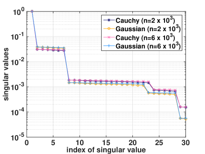
Figure 1: Group patterns in singular values. The singular values are normalized and ordered s.t. $1=\sigma_{1}\geq\sigma_{2}\geq\cdots\geq\sigma_{n}$. The data were randomly generated in dimension 6 with default random seed in MATLAB. The legend shows the data size and the kernel functions: Cauchy ($1/(1+\left\lVert x-y\right\rVert_{2}^{2})$) and Gaussian ($\exp(-\left\lVert x-y\right\rVert_{2}^{2})$).

Second, we observe that the singular values of RBF kernel matrices form groups with plateaus. A pictorial example is in Figure 1. There are 5 groups (plateau) of singular values with a sharp drop in magnitude between groups; the group cardinalities are dependent on the data dimension, but independent of the data size. We explain this phenomenon by applying an appropriate analytic expansion of the function and grouping expansion terms appropriately.

1.3 Organization

This paper is organized as follows. Section 2 presents our theorems concerning the function rank of the approximation of the RBF kernel function, and the $L_{\infty}$ error bound of the approximations. Section 3 provides the theorem proofs. Section 4 shows that for a fixed precision, the polynomial growth rate of the derived rank cannot be improved. Section 5 verifies our theorems experimentally. Finally, in Section 6, we investigate and discuss the group pattern in the singular values of RBF kernel matrices.

2 Main theorems

In this section, we present theorems concerning the function rank and function and data properties. Each theorem approximates the RBF kernels in the $L_{\infty}$ norm with low-rank kernels where the function rank and the error bound are given in explicit formulas. We briefly describe the theorems and then delve into further details.

The first four theorems consider kernels with two types of smoothness assumptions, and for each type, we present the deterministic result and the probabilistic result in two theorems, respectively. The probabilistic results take into account the concentration of measure for large data dimensions. The separable form is obtained by applying a Chebyshev expansion of $f(z)$ followed by a further expansion of $z=\|\mathbf{x}-\mathbf{y}\|_{2}^{2}$.

The key advantage of this approach is that the accuracy of the expansion only depends on $\|\mathbf{x}-\mathbf{y}\|_{2}^{2}$ instead of $(\mathbf{x},\mathbf{y})$, which lies in a $d$-dimensional space. Assume we have expanded $f(z)$ to order $n$ with error $\epsilon$. Then, we substitute $z=\|\mathbf{x}-\mathbf{y}\|_{2}^{2}$, expand the result, and re-arrange the terms to identify the number of distinct separate products of the form $h(\mathbf{x})g(\mathbf{y})$ in the final representation. This number becomes our upper bound on the function rank.

The theorems show that for a fixed precision, the function rank grows polynomially with data dimension $d$, and that the $L_{\infty}$ error for low-rank approximations decreases with decreasing diameter of the domain that contains $\mathbf{x}$ and $\mathbf{y}$.

The last theorem considers kernels with finite smoothness assumptions. The separable form is obtained by applying a Fourier expansion of $f(z)$ followed by a Taylor expansion on each Fourier term. Additional to what the previous theorems suggest, the formulas for the error and the function rank capture subtler relations between different parameters, and the theorem shows that the error decreases when either the diameter of the domain that contains $\mathbf{x}$ or that contains $\mathbf{y}$ decreases. Before presenting our theorems, we introduce some notations.

Notations. Let ${\bf{E}}(\cdot)$ and ${\bf Var}(\cdot)$ denote the expectation and variance, respectively. Let

$$E_{\rho^{2}}=:\Bigl{\{}z=\frac{\rho^{2}e^{\imath\theta}+\rho^{-2}e^{-\imath\theta}}{2}\,\big{|}\,\theta\in[0,2\pi)\Bigr{\}}$$

be the Bernstein ellipse defined on $[-1,1]$ with parameter $\rho^{2}$, an open region bounded by an ellipse. For an arbitrary interval, the ellipse is scaled and shifted and is referred to as the transformed Bernstein ellipse. For instance, given an interval $[a,b]$, let $\phi(x)$ be a linear mapping from $[a,b]$ to $[-1,1]$. And the transformed Bernstein ellipse for $[a,b]$ is defined to be $\phi^{-1}(E_{\rho^{2}})$. In this case, the parameter $\rho^{2}$ still characterizes the shape of the transformed Bernstein ellipse. Therefore, throughout this paper, when we say a transformed Bernstein ellipse with parameter $\rho^{2}$, we refer to the parameter of the Bernstein ellipse defined on [-1, 1]. Let the function domain be $\Omega_{\mathbf{x}}\times\Omega_{\mathbf{y}}\subset\mathbb{R}^{d}\times\mathbb{R}^{d}$, and we refer to $\Omega_{\mathbf{x}}$ as the target domain and $\Omega_{\mathbf{y}}$ as the source domain. We assume the domain is not a manifold, where lower ranks can be expected. Let the sub-domain containing the data of interest be $\widetilde{\Omega}_{\mathbf{x}}\times\widetilde{\Omega}_{\mathbf{y}}\subset\Omega_{\mathbf{x}}\times\Omega_{\mathbf{y}}$.

The following theorems assume the bandwidth parameter $h$ in $\mathcal{K}_{h}(\mathbf{x},\mathbf{y})=f(\|\mathbf{x}-\mathbf{y}\|_{2}^{2}/h^{2})$ to be fixed at 1. A scaled kernel $\mathcal{K}_{h}(\mathbf{x},\mathbf{y})$ will not be considered because it can be handled by rescaling the data points instead. We start with some assumptions on the kernel type, function domain, and probabilistic distribution that will be used in the theorems, and then we present our theorems.

RBF Kernel Assumption.

Consider a function $f$ and kernel function $\mathcal{K}(\mathbf{x},\mathbf{y})=f(\left\lVert\mathbf{x}-\mathbf{y}\right\rVert_{2}^{2})$ with $\mathbf{x}=(x_{1},\ldots,x_{d})$ and $\mathbf{y}=(y_{1},\ldots,y_{d})$. We assume that $x_{i}\in[0,D/\sqrt{d}]$, $y_{i}\in[0,D/\sqrt{d}]$, where $D$ is a constant independent of $d$. And this implies $\|\mathbf{x}-\mathbf{y}\|_{2}^{2}\leq D^{2}$.

Analytic Assumption.

$f$ is analytic in $[0,D^{2}]$, and is analytically continuable to a transformed Bernstein ellipse with parameter $\rho_{D}^{2}>1$, and $|f(x)|\leq C_{D}$ inside the ellipse.

Finite Smoothness Assumption.

$f$ and its derivatives through $f^{(q-1)}$ are absolutely continuous on $[0,D^{2}]$ and the $q$-th derivative has bounded total variation on $[0,D^{2}]$, $V\left(\frac{\,\mathrm{d}^{q}f}{\,\mathrm{d}x^{q}}\right)\leq V_{q}.$

Probability Distribution Assumption.

$x_{i}$ and $y_{i}$ are i.i.d. random variables, with $x_{i}\sqrt{d}\in[0,D]$ and $y_{i}\sqrt{d}\in[0,D]$, and their second moments exist. Let

$$E_{d}=\Big{(}\sum_{i=1}^{d}{\bf E}[(x_{i}-y_{i})^{2}]\Big{)}^{1/2}=\Big{(}2{\bf{E}}[(x_{i}\sqrt{d})^{2}]-2\bigl{(}{\bf{E}}[x_{i}\sqrt{d}]\bigr{)}^{2}\Big{)}^{1/2}$$

and

$$\sigma_{d}^{2}=\sum_{i=1}^{d}{\bf Var}[(x_{i}-y_{i})^{2}]$$

Then, $E_{d}\in\Theta(1)$ with respect to $d$, i.e., the mean distance between pairs of points neither goes to 0 nor $\infty$ with $d$. And $\sigma_{d}^{2}\in\Theta(\frac{1}{d})$ (a concentration of measure).

Theorem 2.1.

Suppose the RBF Kernel Assumption and the Analytic Assumption hold. Then, for $n\geq 0$, the kernel $\mathcal{K}$ can be approximated in the $L_{\infty}$ norm by a low-rank kernel $\widetilde{\mathcal{K}}$ of function rank at most $R(n,d)=\binom{n+d+2}{d+2}$

$$\mathcal{K}(\mathbf{x},\mathbf{y})=\sum_{i=1}^{R}g_{i}(\mathbf{x})h_{i}(\mathbf{y})+\epsilon_{n}=\widetilde{\mathcal{K}}(\mathbf{x},\mathbf{y})+\epsilon_{n}$$ (1)

where $\{g_{i}\}_{i=1}^{R}$ and $\{h_{i}\}_{i=1}^{R}$ are two sequences of $d$-variable polynomials. And the error term $\epsilon_{n}=\epsilon_{n}(D)$ is bounded as

$$|\epsilon_{n}(D)|\leq\frac{2C_{D}\rho_{D}^{-2n}}{\rho_{D}^{2}-1}$$ (2)

Remark. If an approximation with a given maximal rank $r$ is requested, we need to select an $n(r,d)$ such that $\binom{n(r,d)+d+2}{d+2}\leq r$. Then, we obtain an approximation with error $|\epsilon_{n}(D)|\leq\frac{2C_{D}\rho_{D}^{-2n}}{\rho_{D}^{2}-1}$ and function rank at most $\binom{n(r,d)+d+2}{d+2}\leq r$. The low-rank kernel $\widetilde{\mathcal{K}}$ is of order $2n$, which can be revealed from the explicit form of $\widetilde{\mathcal{K}}$ in the proof (see Section 3.2). For the space of $d$-variate polynomials with maximum total degree $2n$, the dimension is $\binom{2n+d}{d}$. In contrast, our upper bound is $\binom{n+d+2}{d+2}$. When $d\geq 4$, our formula becomes favorable for a large range of $k$.

Corollary 2.2.

Under the same assumptions in Theorem 2.1 and with $n$ fixed, the low-rank kernel approximation, for a fixed precision $\epsilon$, is achievable with a rank proportional to $d^{\frac{-\log c_{1}\epsilon}{c_{2}}}$, where $c_{1}$ and $c_{2}$ are positive constants.

The proofs of Theorem 2.1 and Corollary 2.2 can be found in Section 3.1 and Section 3.2, respectively.

Theorem 2.1 suggests that for some precision $\epsilon$, the function rank grows polynomially with increasing data dimension $d$, i.e., $R=O(d^{n})$, where $n$ is determined by the desired precision $\epsilon$, $D,\rho_{D}$ and $C_{D}$. This can be seen from $R=\binom{n+d+2}{d+2}$ with $n$ fixed and $d\rightarrow\infty$.

For a fixed $n$ and for a sub-domain $\widetilde{\Omega}_{\mathbf{x}}\cup\widetilde{\Omega}_{\mathbf{y}}$ with diameter $\tilde{D}<D$, the error bound decreases, namely in the following sense. In this case, the same function $f$ on the sub-domain can be analytically extended to a Bernstein ellipse whose parameter is larger than $\rho_{D}^{2}$, reducing the error bound in Eq. 2. Therefore, when the diameter of the domain that contains our data decreases, we will observe a lower approximation error for low-rank approximations with a fixed function rank, and similarly, we will observe a lower function rank for low-rank approximations with a fixed accuracy.

Along the same line of reasoning, for a fixed kernel on a fixed domain, when the point sets become denser, we should expect the function rank to remain unchanged for a fixed precision. The result for function ranks turns out to be in perfect agreement with the observations in practical situations on matrix ranks, assuming there are sufficiently many points to make the matrix rank visible before reaching a given precision.

We now turn to the case when $d$ is large. Because we have assumed $x_{i}$ and $y_{i}$ to be in $[0,D/\sqrt{d}]$, by concentration of measure, the values of $\|\mathbf{x}-\mathbf{y}\|_{2}^{2}$ will fall into a small-sized subinterval of $[0,D^{2}]$ with high probability. Therefore, we are interested in quantifying this probabilistic error bound.

Theorem 2.3.

Suppose the RBF Kernel Assumption and the Analytic Assumption hold, and points $\mathbf{x}$ and $\mathbf{y}$ are sampled under the probability distribution involving $D$, $\sigma_{d}$ and $E_{d}$ in Probability Distribution Assumption. We define function $\tilde{f}(x-E_{d}^{2})=f(x)$. Then, $\tilde{f}$ is analytic in $[-E_{d}^{2},D^{2}-E_{d}^{2}]$, with the parameter of its transformed Bernstein ellipse to be $\tilde{\rho}_{D}^{2}>1$, and $|\tilde{f}(x)|\leq\tilde{C}_{D}$ inside the ellipse. Defining the same error $\epsilon_{n}$ as in Theorem 2.1

$$\epsilon_{n}(D,\delta)=\mathcal{K}(\mathbf{x},\mathbf{y})-\sum_{i=1}^{R}g_{i}(\mathbf{x})h_{i}(\mathbf{y}),\,\,\text{with }R=\binom{n+d+2}{d+2}$$ (3)

we obtain that for $0<\delta<D$, with probability at least

$$1-2\exp\left(\frac{-\delta^{4}\,d}{2\sigma_{d}^{2}\,d+8D^{2}\delta^{2}/3}\right)$$ (4)

the error can be bounded by

$$|\epsilon_{n}(D,\delta)|\leq\frac{2C_{D}\delta^{2}}{D^{2}(\tilde{\rho}_{D}^{2}-\tilde{\rho}_{D}^{-2})-\delta^{2}}\left(\frac{D^{2}(\tilde{\rho}_{D}^{2}-\tilde{\rho}_{D}^{-2})}{\delta^{2}}\right)^{-n}$$

And with the same probability, the distance of a sampled pair will fall into the following interval

$$\|\mathbf{x}-\mathbf{y}\|_{2}^{2}\in[E_{d}^{2}-\delta^{2},E_{d}^{2}+\delta^{2}]$$

The proof of Theorem 2.3 can be found in Section 3.3.

In Theorem 2.3, as $d\to\infty$, $\delta$ needs to decrease with $d$ to maintain the same probability. If we choose $\delta=\left(\frac{C}{d}\right)^{1/4}$ with $C$ being a very large number, then the probability remains close to 1 because $\sigma_{d}^{2}=\Theta(\frac{1}{d})$. Moreover, we can keep $\epsilon_{n}$ small while reducing $n$, because $\delta\to 0$. This means that for sufficiently large $d$ and for a given error, $n$ goes down as $d$ increases. Asymptotically, $n$ reaches 0, and the function rank reaches 1. On the other hand, for a fixed $n$, the error bound decreases when $d$ increases.

Note that $2\delta^{2}$ is the size of the subinterval where the values of $\left\lVert\mathbf{x}-\mathbf{y}\right\rVert_{2}^{2}$’s fall into with probability given by Eq. 4 and, by concentration of measure, with the same probability, the interval size $2\delta^{2}$ shrinks with increasing $d$. This is consistent with what we have discussed that $\delta$ needs to decrease with $d$ to maintain the same probability.

The analytic assumption in Theorem 2.1 and Theorem 2.3 is very strong because many RBFs are not infinitely differentiable when the domain contains zero. However, most RBFs of practical interest are $q$-times differentiable. In the following theorem, we weaken the analytic assumption to a finite-smoothness assumption and compute the corresponding error bound.

Theorem 2.4.

Suppose the RBF Kernel Assumption and the Finite Smoothness Assumption hold. Then for $n>q$, the kernel $\mathcal{K}$ can be approximated in the $L_{\infty}$ norm by a low-rank kernel $\widetilde{\mathcal{K}}$ of function rank at most $R(n,d)=\binom{n+d+2}{d+2}$

$$\mathcal{K}(\mathbf{x},\mathbf{y})=\sum_{i=1}^{R}g_{i}(\mathbf{x})h_{i}(\mathbf{y})+\epsilon_{n}=\widetilde{\mathcal{K}}(\mathbf{x},\mathbf{y})+\epsilon_{n}$$

where $\{g_{i}\}_{i=1}^{R}$ and $\{h_{i}\}_{i=1}^{R}$ are two sequences of $d$-variable polynomials. And the error term $\epsilon_{n}=\epsilon_{n}(V_{q},D,q)$ is bounded as

$$|\epsilon_{n}(V_{q},D,q)|\leq\frac{2V_{q}D^{2q}}{\pi q[2(n-q)]^{q}}$$ (5)

Remark. We can weaken the assumption of $f^{(q)}$ having bounded total variation to $f^{(q-1)}$ being Lipschitz continuous, and this does not impose assumptions on $f^{(q)}$. With this weaker assumption, we obtain the same error rate $O(n^{-q})$; however, the trade off is the absent of explicit constants in the upper bound Eq. 5.

The proof of Theorem 2.4 can be found in Section 3.4.

Compared to Theorem 2.1, the convergence rate slows down from a nice geometric convergence rate $O(\rho_{D}^{-2n})$ to an algebraic convergence rate $O(n^{-q})$. Each time the function becomes one derivative smoother ($q$ increased by 1), the convergence rate will also become one order faster. The domain diameter $D$ affects the error bound by $D^{2q}$, where $q$ represents the smoothness of the function. For a sub-domain with diameter $\widetilde{D}$, it is straightforward to obtain that the error is bounded by $\frac{2V_{q}\widetilde{D}^{2q}}{\pi q[2(n-q)]^{q}}$, and for a fixed $n$, a decrease in $\widetilde{D}$ will reduce the error.

We also consider the phenomenon of concentration of measure and present the probabilistic result in the following theorem. $x_{i}$ and $y_{i}$ are i.i.d. random variables, with $|x_{i}\sqrt{d}|<D$ and $|y_{i}\sqrt{d}|<D$, and have their second moments exist.

Theorem 2.5.

Suppose the RBF Kernel Assumption and the Finite Smoothness Assumption hold. We further assume $\mathbf{x}$ and $\mathbf{y}$ are sampled under the probability distribution involving $D$, $E_{d}$, and $\sigma_{d}$ in Probability Distribution Assumption. Defining the same $\epsilon_{n}$ as in Theorem 2.4

$$\epsilon_{n}(V_{q},\delta,q)=\mathcal{K}(\mathbf{x},\mathbf{y})-\sum_{i=1}^{R}g_{i}(\mathbf{x})h_{i}(\mathbf{y}),\quad\text{with }R=\binom{n+d+2}{d+2}$$

Then, for $0<\delta<D$, we obtain the following bound

$$|\epsilon_{n}(V_{q},\delta,q)|\leq\frac{2V_{q}\delta^{2q}}{\pi q[2(n-q)]^{q}}$$

with probability at least

$$1-2\exp\left(\frac{-\delta^{4}\,d}{2\sigma_{d}^{2}\,d+8D^{2}\delta^{2}/3}\right)$$

The proof of Theorem 2.5 can be found in Section 3.4.

Up to now, we have only considered a single parameter $D$ that characterizes the domain, to make the error bound more informative as in response to subtler changes of the domain, we also consider the diameters of the target domain $D_{\mathbf{x}}$ and of the source domain $D_{\mathbf{y}}$. The following theorem nicely quantifies the influences of $D_{\mathbf{x}}$ and $D_{\mathbf{y}}$ on the error. Our result theoretically offers critical insights and motivations for many algorithms that take advantage of the low-rank property of sub-matrices, where these sub-matrices usually relate to data clusters of small diameters.

Theorem 2.6.

Suppose the RBF Kernel Assumption hold, and there are $D_{\mathbf{x}}<D$ and $D_{\mathbf{y}}<D$, such that $\|\mathbf{x}_{i}-\mathbf{x}_{j}\|_{2}\leq D_{\mathbf{x}}$ and $\|\mathbf{y}_{i}-\mathbf{y}_{j}\|_{2}\leq D_{\mathbf{y}}$.

Let $f_{p}(x)=\sum_{n}\mathcal{T}\circ f(x+4nD^{2})$ be a $4D^{2}$-periodic extension of $f(x)$, where $\mathcal{T}(\cdot)$ is 1 on $[-D^{2},D^{2}]$ and smoothly decays to 0 outside of the interval. We assume that $f_{p}$ and its derivatives through $f_{p}^{(q-1)}$ are continuous, and the $q$-th derivative is piecewise continuous with the total variation over one period bounded by $V_{q}$.

Then, for $M_{f},M_{t}>0$ with $9M_{f}\leq M_{t}$, the kernel $\mathcal{K}$ can be approximated by a low-rank kernel $\widetilde{\mathcal{K}}$ of rank at most $R(M_{f},M_{t},d)=4M_{f}\binom{M_{t}+d}{d}$

$$\mathcal{K}(\mathbf{x},\mathbf{y})=\sum_{i=1}^{R}g_{i}(\mathbf{x})h_{i}(\mathbf{y})+\epsilon_{M_{f},M_{t}}=\widetilde{\mathcal{K}}(\mathbf{x},\mathbf{y})+\epsilon_{M_{f},M_{t}}$$

And the error $\epsilon_{M_{f},M_{t}}=\epsilon_{M_{f},M_{t}}(D_{\mathbf{x}},D_{\mathbf{y}},q,\rho)$ is bounded by

$$|\epsilon_{M_{f},M_{t}}(D_{\mathbf{x}},D_{\mathbf{y}},q,\rho)|\leq\left\lVert f\right\rVert_{\infty}\left(\frac{D_{\mathbf{x}}D_{\mathbf{y}}}{D^{2}}\right)^{M_{t}+1}+\frac{V_{q}}{\pi q}\left(\frac{2D^{2}}{\pi M_{f}}\right)^{q}$$

The proof of Theorem 2.6 can be found in Section 3.5.

In contrast to the previous theorems where the domain information only enters the error as $D$, in Theorem 2.6, the diameters of the source domain $D_{\mathbf{y}}$ and the target domain $D_{\mathbf{x}}$ also appear in error. The form $\left(\frac{D_{\mathbf{x}}D_{\mathbf{y}}}{D^{2}}\right)^{M_{t}+1}$ suggests that a decrease in $\frac{D_{\mathbf{x}}D_{\mathbf{y}}}{D^{2}}$ will reduce the error, which can be achieved when either the source or the target domain has a smaller diameter. This property has motivated people to approach matrix approximation problems by identifying low-rank blocks in a matrix, which is partially achieved by partitioning the data into clusters of small diameters.

The function rank still remains a polynomial growth and it grows as $R=O(d^{M_{t}})$, when $M_{f}$ and $M_{t}$ are fixed and $d\rightarrow\infty$. $M_{f}$ represents the Fourier expansion order of $f$, and each term in the expansion is further expanded into Taylor terms up to order $M_{t}$. We assumed $M_{t}$ to be the same across all the Fourier terms for simplicity. If we decrease the Taylor order $M_{t}$ with increasing Fourier order to preserve more information of low-order Fourier terms, then a lower error bound can be attained for the same function rank.

Remark. We summarize the assumptions, error bounds and function ranks of the theorems in Table 1, and discuss the similarities and differences in the function rank and the error bound. We refer to Theorem 2.1 and Theorem 2.4 as the Chebyshev approach and Theorem 2.6 as the Fourier-Taylor approach based on their proof techniques. The function rank is determined by the data dimension and the expansion order, and it is a power of the dimension, where the power is the expansion order and is different in the Chebyshev approach and the Fourier-Taylor approach. The error bounds quantify the influences from the expansion order and the domain diameter: a higher expansion order reduces the error bound, so does a smaller domain diameter. The domain diameter occurs as a single parameter $D$ in the Chebyshev approach but as $D_{\mathbf{x}}$, $D_{\mathbf{y}}$ and $D$ in the Fourier-Taylor approach.

From the practical viewpoint, the absence of exponential growth for the function rank agrees with the practical situation where people observe lower matrix ranks for high dimension data. And, the fact that decreasing $D_{\mathbf{x}}$ or $D_{\mathbf{y}}$ reduces the error is also in agreement with practice and moreover, it provides an insight of why point clusterings followed by local interpolations often leads to a more memory efficient approximation.

Table 1: Theorem Summary

Approach Chebyshev expansion + Exact expansion of $\left\lVert\mathbf{x}-\mathbf{y}\right\rVert^{2l}$ Fourier expansion + Taylor expansion of $\exp{(\imath\mathbf{x}^{T}\mathbf{y})}$ Deterministic (analytic) Probabilistic (analytic) Deterministic (finite smoothness) Probabilistic (finite smoothness) Deterministic (finite smoothness) Condition • RBF Kernel Assumption • Analytic Assumption • RBF Kernel Assumption • Analytic Assumption • $\tilde{f}(x-E_{d}^{2})=f(x)$ with parameter of its transformed Bernstein ellipse to be $\tilde{\rho}_{D}^{2}>1$ • Probability Distribution Assumption • RBF Kernel Assumption • Finite Smoothness Assumption • RBF Kernel Assumption • Finite Smoothness Assumption • Probability Distribution Assumption • RBF Kernel Assumption • $f_{p}(x)$ is the $4D^{2}$-periodic extension of $f$ and $\|f(x)-f_{p}(x)\|_{\infty,[-D^{2},D^{2}]}=0$ • The first $q-1$ derivatives of $f_{p}$ are continuous, and the $q$-th derivative on $[-D^{2},D^{2}]$ is piece-wise continuous with bounded total variation $V_{q}$ • $9M_{f}\leq M_{t}$ Error $\dfrac{2C_{D}\rho_{D}^{-2n}}{\rho_{D}^{2}-1}$ $\dfrac{2C_{D}\delta^{2}}{D^{2}\Big{(}\tilde{\rho}_{D}^{2}-\tilde{\rho}_{D}^{-2}\Big{)}-\delta^{2}}\times$
$\left(\dfrac{D^{2}\Big{(}\tilde{\rho}_{D}^{2}-\tilde{\rho}_{D}^{-2}\Big{)}}{\delta^{2}}\right)^{-n}$ with probability at least $Pr(\delta,D,\sigma_{d},d)$ for $0<\delta<D$ $\dfrac{2V_{q}D^{2q}}{\pi q[2(n-q)]^{q}}$ $\dfrac{2V_{q}\delta^{2q}}{\pi q[2(n-q)]^{q}}$ with probability at least $Pr(\delta,D,\sigma_{d},d)$ for $0<\delta<D$ $\left\lVert f\right\rVert_{\infty}\left(\dfrac{D_{\mathbf{x}}D_{\mathbf{y}}}{D^{2}}\right)^{M_{t}+1}+\dfrac{V_{q}}{\pi q}\left(\dfrac{2D^{2}}{\pi M_{f}}\right)^{q}$ Rank $\binom{n+d+2}{d+2}$ $4M_{f}\binom{M_{t}+d}{d}$ Notation $n$: Chebyshev expansion order
$D$: $\left\lVert\mathbf{x}-\mathbf{y}\right\rVert_{2}<D$
$E_{d}^{2}=\sum_{i=1}^{d}{\bf E}[(x_{i}-y_{i})^{2}]$
$\sigma_{d}^{2}=\sum_{i=1}^{d}{\bf Var}[(x_{i}-y_{i})^{2}]$
$Pr(\delta,D,\sigma_{d},d)=1-2\exp\left(\dfrac{-\delta^{4}\,d}{2\sigma_{d}^{2}\,d+8D^{2}\delta^{2}/3}\right)$ $D_{\mathbf{x}}$: $\left\lVert\mathbf{x}_{i}-\mathbf{x}_{j}\right\rVert_{2}<D_{\mathbf{x}}$
$D_{\mathbf{y}}$: $\left\lVert\mathbf{y}_{i}-\mathbf{y}_{j}\right\rVert_{2}<D_{\mathbf{y}}$
$M_{f}$: Fourier expansion order
$M_{t}$: Taylor expansion order

3 Theorem Proofs

In this section, we prove the theorems in Section 2. All the proofs consist of three components: separating $\mathcal{K}(\mathbf{x},\mathbf{y})$ into a finite sum of products of real-valued functions $h_{i}(\mathbf{x})g_{i}(\mathbf{y})$, counting the terms to obtain an upper bound for the function rank, and calculating the error bound. Similar techniques can be found in [26, 33, 40, 44]. We describe the high-level procedure of the separation step; the rest steps should be straightforward.

In the proofs of Theorem 2.1 and Theorem 2.4, the separable form was obtained by first expanding the kernel into polynomials of $z=\left\lVert\mathbf{x}-\mathbf{y}\right\rVert^{2}$ of a certain order to settle the error bound, and then expanding the terms $\left\lVert\mathbf{x}-\mathbf{y}\right\rVert^{2l}$. The key advantage of this approach has been discussed at the beginning of Section 2. We seek approximation theorems in 1D that provide optimal convergence rate and explicit error bounds. Chebyshev theorems (Theorem 8.2 and Theorem 7.2 in [36]) are ideal choices. Analogous results also exist, e.g., the classic Bernstein and Jackson’s approximation theorems (page 257 in [3]), but the downside is that they only provide an error rate rather than an explicit formula, and moreover, they will not improve our results or simplify the proofs.

In the proof of Theorem 2.6, the separable form was obtained by first applying a Fourier expansion on $\mathcal{K}$ to separate the cross term $\exp(\mathbf{x}^{T}\mathbf{y})$, then applying a Taylor expansion on the cross term.

Before stating the detailed proofs, we introduce some notations that will be used.
Notations. For multi-index ${\bm{\alpha}}=[\alpha_{1},\cdots,\alpha_{d}]\in\mathbb{N}^{d}$ and vector $\mathbf{x}=[x_{1},\cdots,x_{d}]\in\mathbb{R}^{d}$, we define $|{{\bm{\alpha}}}|=\alpha_{1}+\alpha_{2}+\cdots+\alpha_{d}$, $\mathbf{x}^{{\bm{\alpha}}}=x_{1}^{\alpha_{1}}x_{2}^{\alpha_{2}}\cdots x_{d}^{\alpha_{d}}$ and the multinomial coefficient with $|{\bm{\alpha}}|=m$ to be $\binom{m}{{\bm{\alpha}}}=\frac{m!}{\alpha_{1}!\alpha_{2}!\cdots\alpha_{d}!}.$

3.1 Proof of Theorem 2.1

We first introduce a lemma on the identity of binomial coefficients.

Lemma 3.1.

For $d\in\mathbb{Z}^{+}$ and $m\in\mathbb{Z}$, the following identity holds:

$$\sum_{k=0}^{m}\binom{k+d}{d}=\binom{m+1+d}{d+1}$$

Proof.

The proof can be done by induction and follows that from Lemma 2.4 in [41]. ∎

Proof.

The proof consists of two components. First, we map the domain of $f$ to $[0,2]$ (for the convenience of the proof) and approximate $f$ with a Chebyshev polynomial, and this settles the error. Second, we further separate terms $\left\lVert\mathbf{x}-\mathbf{y}\right\rVert^{2}$ in the polynomial and count the number of distinct terms to be an upper bound of the function rank.

• Approximation by Chebyshev polynomials. We first linearly map the domain of $f$ to $[0,2]$ and denote the new function as $\tilde{f}$:

  $$\mathcal{K}(\mathbf{x},\mathbf{y})=f(\left\lVert\mathbf{x}-\mathbf{y}\right\rVert_{2}^{2})=\tilde{f}\left(\frac{2}{D^{2}}\left\lVert\mathbf{x}-\mathbf{y}\right\rVert_{2}^{2}\right)=\tilde{f}(z)$$ (6)

  Because $\left\lVert\mathbf{x}-\mathbf{y}\right\rVert^{2}\in[0,D^{2}]$, it follows that $z\in[0,2]$. From our assumptions, $\tilde{f}$ is analytic in $[0,2]$ and is analytically continuable to the open Bernstein ellipse with parameter ${\rho_{D}^{2}}$ (consider a shifted ellipse).

  According to Theorem 8.2 in [36] that follows from [24], for $n\geq 0$, we can approximate $\tilde{f}$ by its Chebyshev truncations $\tilde{f}_{n}$ in the $L_{\infty}$ norm with error

  $$|\epsilon_{n}|\leq\frac{2C_{D}\rho_{D}^{-2n}}{\rho_{D}^{2}-1}$$ (7)

  and

  $$\begin{split}{\tilde{f}}_{n}(z)=\sum_{k=0}^{n}c_{k}T_{k}(z)+\epsilon_{n}\end{split}$$ (8)

  where $c_{k}=\frac{2}{\pi}\bigintsss_{-1}^{1}\frac{{\tilde{f}}(z)T_{k}(z)}{\sqrt{1-z^{2}}}dz$, and $T_{k}(z)$ is the Chebyshev polynomial of the first kind of degree $k$ defined by the relation:

  $$T_{k}(x)=\cos(k\theta),~{}\text{with}~{}x=\cos(\theta).$$ (9)

  Rearranging the terms in Eq. 8 we obtain a polynomial of $z=\left\lVert\mathbf{x}-\mathbf{y}\right\rVert^{2}$:

  $$\mathcal{K}(\mathbf{x},\mathbf{y})={\tilde{f}}\left(\frac{2}{D^{2}}\left\lVert\mathbf{x}-\mathbf{y}\right\rVert_{2}^{2}\right)=\sum_{k=0}^{n}\frac{a_{k}}{D^{2k}}\left\lVert\mathbf{x}-\mathbf{y}\right\rVert^{2k}+\epsilon_{n}$$ (10)

  where $a_{k}$ depends on $c_{k}$ but is independent of $\mathbf{x}$ and $\mathbf{y}$.

• Separable form. We separate each term $\left\lVert\mathbf{x}-\mathbf{y}\right\rVert^{2l}$ in Eq. 10 into a finite sum of separate products:

  $$\begin{split}\|\mathbf{x}-\mathbf{y}\|^{2l}&=\sum_{k=0}^{l}{l\choose k}(-2)^{l-k}\sum_{j=0}^{k}{k\choose j}\left\lVert\mathbf{x}\right\rVert^{2j}\left\lVert\mathbf{y}\right\rVert^{2(k-j)}\left(\sum_{i=1}^{d}x_{i}y_{i}\right)^{l-k}\\ &=\sum_{k=0}^{l}\sum_{j=0}^{k}\sum_{|{\bm{\alpha}}|=l-k}C_{l,k,{\bm{\alpha}}}\left(\left\lVert\mathbf{x}\right\rVert^{2j}\mathbf{x}^{{\bm{\alpha}}}\right)\left(\left\lVert\mathbf{y}\right\rVert^{2(k-j)}\mathbf{y}^{{\bm{\alpha}}}\right)\end{split}$$ (11)

  where $C_{l,k,{\bm{\alpha}}}=(-2)^{l-k}\binom{l}{k}\binom{k}{j}\binom{l-k}{{\bm{\alpha}}}$. Substituting Eq. 11 into Eq. 10, we obtain a separable form of $\mathcal{K}$:

  $$\mathcal{K}(\mathbf{x},\mathbf{y})=\sum_{l=0}^{n}\sum_{k=0}^{l}\sum_{j=0}^{k}\sum_{|{\bm{\alpha}}|=l-k}D_{l,k,{\bm{\alpha}}}\left(\left\lVert\mathbf{x}\right\rVert^{2j}\mathbf{x}^{{\bm{\alpha}}}\right)\left(\left\lVert\mathbf{y}\right\rVert^{2(k-j)}\mathbf{y}^{{\bm{\alpha}}}\right)+\epsilon_{n}$$ (12)

  where $D_{l,k,{\bm{\alpha}}}=\frac{a_{l}}{D^{2l}}(-2)^{l-k}\binom{l}{k}\binom{k}{j}\binom{l-k}{{\bm{\alpha}}}$ is a constant independent of $\mathbf{x}$ and $\mathbf{y}$. Therefore, the function rank of $\mathcal{K}$ can be upper bounded by the total number of separate terms:

  $$\sum_{l=0}^{n}\sum_{k=0}^{l}(k+1)\binom{l-k+d-1}{d-1}=\binom{n+d+2}{d+2}$$

  where the equality follows from the result in Lemma 3.1. To summarize, we have proved that $\mathcal{K}(\mathbf{x},\mathbf{y})$ can be approximated by the separable form in Eq. 12 in the $L_{\infty}$ norm with rank at most

  $$R(n,d)=\binom{n+d+2}{d+2}$$ (13)

  and approximation error

  $$|\epsilon_{n}(D)|\leq\frac{2C_{D}\rho_{D}^{-2n}}{\rho_{D}^{2}-1}$$ (14)

∎

3.2 Proof of Corollary 2.2

Proof.

For a fixed kernel function and fixed $n$, we define two constants $c_{1}=\frac{\rho_{D}^{2}-1}{2C_{D}}$ and $c_{2}=\log\rho_{D}^{2}$. Then, the truncation error $\epsilon$ can be rewritten as

$$\epsilon=\frac{2C_{D}\rho_{D}^{-2n}}{\rho_{D}^{2}-1}=\frac{e^{-nc_{2}}}{c_{1}}$$

and equivalently,

$$n=\frac{-\log c_{1}\epsilon}{c_{2}}$$ (15)

We relate function rank $R$ to error $\epsilon$ and dimension $d$. When $d\geq n+2$, we obtain,

$$\begin{split}R&=\binom{n+d+2}{d+2}\leq\frac{2^{n}d^{n}}{n!}=c_{n}d^{\frac{-\log c_{1}\epsilon}{c_{2}}}\\ \end{split}$$ (16)

where $c_{n}=\frac{2^{n}}{n!}$ is a constant for a fixed $n$. Therefore, an $\epsilon$ error is achievable with the function rank $R$ proportional to $d^{\frac{-\log c_{1}\epsilon}{c_{2}}}$. ∎

3.3 Proof of Theorem 2.3

Proof.

We consider the concentration of measure phenomenon and apply concentration inequalities to obtain a probabilistic error bound. The proof mostly follows the proof of Theorem 2.1, and we will focus on computing the error bound for a smaller domain.

To simplify the proof, we consider a function $\tilde{f}$ that is shifted by $E_{d}^{2}$ such that

$$f(\left\lVert\mathbf{x}-\mathbf{y}\right\rVert_{2}^{2})={\tilde{f}}(\left\lVert\mathbf{x}-\mathbf{y}\right\rVert_{2}^{2}-E_{d}^{2})$$

and we will see later that this shift ensures the inputs for $\tilde{f}$ to fall into an interval that centers around 0 with some probability. $\tilde{f}$ inherits the analyticity of $f$; therefore, it is analytic on $[-E_{d}^{2},D^{2}-E_{d}^{2}]$, and can be analytically extended to a transformed Bernstein Ellipse with parameter $\tilde{\rho}_{D}^{2}$.

Let us denote $z_{i}=(x_{i}-y_{i})^{2}-{\bf E}[(x_{i}-y_{i})^{2}]$ and we will shortly apply concentration inequality to $z_{i}$. With the assumptions that $x_{i}\sqrt{d}$ and $y_{i}\sqrt{d}$ are i.i.d. random variables where $|x_{i}\sqrt{d}|<D$ and $|y_{i}\sqrt{d}|<D$, it follows that the $z_{i}$ are statistically independent with mean zero and are bounded by $\frac{4D^{2}}{d}$. By applying Bernstein’s inequality [4] on the sum of the $z_{i}$, we conclude that for $\delta\geq 0$,

$$P\left(|\left\lVert\mathbf{x}-\mathbf{y}\right\rVert_{2}^{2}-E_{d}^{2}|\leq\delta^{2}\right)\geq 1-2\exp\left(\frac{-\delta^{4}\,d}{2\sigma_{d}^{2}\,d+8D^{2}\delta^{2}/3}\right)$$ (17)

where $E_{d}^{2}=\sum_{i=1}^{d}{\bf E}[(x_{i}-y_{i})^{2}]$ is a constant. In other words, $\left\lVert\mathbf{x}-\mathbf{y}\right\rVert_{2}^{2}\in[E_{d}^{2}-\delta^{2},E_{d}^{2}+\delta^{2}]$ with probability at least

$$1-2\exp\left(\frac{-\delta^{4}\,d}{2\sigma_{d}^{2}\,d+8D^{2}\delta^{2}/3}\right)$$

This also means that with the same probability in Eq. 17, the inputs for $\tilde{f}$ will fall into the interval $[-\delta^{2},\delta^{2}]$.

Therefore, for a probability associated with $\delta$, we can turn to considering $\tilde{f}$ on the domain $[-\delta^{2},\delta^{2}]$. We assume that $\tilde{f}$ is analytically extended to a transformed Bernstein ellipse with parameter $\rho_{\delta}^{2}$, with the value of $\tilde{f}(z)$ inside the ellipse bounded by $C_{\delta}$. Following the same argument in the proof for Theorem 2.1, we obtain that for $\delta>0$ and with probability in Eq. 17, the approximation error for $\mathbf{x}$ and $\mathbf{y}$ sampled from the above distribution is bounded by

$$|\epsilon_{n}|\leq\frac{2C_{\delta}}{\rho_{\delta}^{2}-1}\rho_{\delta}^{-2n}$$ (18)

This sharper bound can be achieved with the same function rank as in Eq. 13 and with the same low-rank representation as in Eq. 12 except for coefficients.

Next, we rewrite the upper bound in Eq. 18 with the parameters $\tilde{\rho}_{D}$, $\tilde{C}_{D}$, and $\delta$. If we linearly map the domain of $\tilde{f}$ from $[-\delta^{2},\delta^{2}]$ to [-1,1], then the Bernstein ellipse with parameter $\tilde{\rho}_{D}^{2}$ will be scaled by $\frac{1}{\delta^{2}}$. We seek the largest $\rho_{\delta}^{2}$ such that the Bernstein ellipse with parameter $\rho_{\delta}^{2}$ will be contained in the transformed Bernstein ellipse with parameter $\tilde{\rho}_{D}^{2}$. In that case, the lengths of their semi-minor axises match and the largest $\rho_{\delta}^{2}$ satisfies

$$\rho_{\delta}^{2}-\rho_{\delta}^{-2}=\frac{D^{2}}{\delta^{2}}\left(\tilde{\rho}_{D}^{2}-\tilde{\rho}_{D}^{-2}\right)$$ (19)

and we obtain $\rho_{\delta}^{2}=\frac{D^{2}}{\delta^{2}}(\tilde{\rho}_{D}^{2}-\tilde{\rho}_{D}^{-2})+\left(\frac{D^{4}}{4\delta^{4}}(\tilde{\rho}_{D}^{2}-\tilde{\rho}_{D}^{-2})^{2}+1\right)^{\frac{1}{2}}$. In the special case where $\delta^{2}=D^{2}$, $\rho_{\delta}^{2}=\tilde{\rho}_{D}^{2}$, we recover the error bound $\frac{2C_{D}}{\tilde{\rho}_{D}^{2}-1}\tilde{\rho}_{D}^{-2n}$. To simplify the bound, we use the relation that $\rho_{\delta}^{2}>\frac{D^{2}}{\delta^{2}}(\tilde{\rho}_{D}^{2}-\tilde{\rho}_{D}^{-2})$. Substituting this into Eq. 18, along with the fact that $C_{\delta}\leq C_{D}$, we obtain

$$|\epsilon_{n}|\leq\frac{2C_{D}\delta^{2}}{D^{2}(\tilde{\rho}_{D}^{2}-\tilde{\rho}_{D}^{-2})-\delta^{2}}\left(\frac{D^{2}(\tilde{\rho}_{D}^{2}-\tilde{\rho}_{D}^{-2})}{\delta^{2}}\right)^{-n}$$ (20)

Therefore, the function rank related to error $\epsilon_{n}$ remains $\binom{n+d+2}{d+2}$, and we have proved our result. ∎

3.4 Proof of Theorem 2.4 and Theorem 2.5

Proof.

The proof follows the same steps as that in Theorem 2.1 and Theorem 2.3; we only need to establish that the error term in the Chebyshev expansion is bounded by $\frac{2D^{2q}V_{q}}{\pi q[(n-q)]^{q}}$. Consider Eq. 6. Because $f^{(q)}$ is piecewise continuous with its total variation on $[0,D^{2}]$ bounded by $V_{q}$, it follows that ${\tilde{f}}^{(q)}$ in Eq. 6 is piecewise continuous on $[0,2]$, with its total variation on $[0,2]$ bounded as follows

$$V\left(\frac{\,\mathrm{d}^{q}{\widetilde{f}}}{\,\mathrm{d}x^{q}}\right)=V\left(\frac{D^{2q}}{2^{q}}\frac{\,\mathrm{d}^{q}f}{\,\mathrm{d}^{q}x^{q}}\right)=\frac{D^{2q}}{2^{q}}V\left(\frac{\,\mathrm{d}^{q}f}{\,\mathrm{d}^{q}x^{q}}\right)\leq\frac{D^{2q}}{2^{q}}V_{q}$$

Therefore, by Theorem 7.2 in [36], for $n>q$, the order-$n$ Chebyshev expansion ${\tilde{f}}_{n}$ approximates $\tilde{f}$ in the $L_{\infty}$ norm with error bounded by

$$|\epsilon_{n}|\leq\frac{2V_{q}({\tilde{f}})}{\pi q(n-q)^{q}}\leq\frac{2D^{2q}V_{q}}{\pi q(2(n-q))^{q}}$$

The rest of the proof is identical to that of Theorem 2.1 for the deterministic result, and identical to that of Theorem 2.3 for the probabilistic result. ∎

3.5 Proof of Theorem 2.6

We first introduce a lemma concerning the function rank of complex functions.

Lemma 3.2.

If a real-valued function $\mathcal{K}$ can be approximated by two sequences of complex-valued functions, i.e.,

$$\left|\mathcal{K}(\mathbf{x},\mathbf{y})-\sum_{i=1}^{R_{c}}\Psi_{i}(\mathbf{x})\Phi_{i}(\mathbf{y})\right|\leq\epsilon,\quad\mathbf{x}\in\Omega_{\mathbf{x}},\mathbf{y}\in\Omega_{\mathbf{y}}$$

where $\{\Psi_{i}(\mathbf{x})\}_{i=1}^{R_{c}}$ and $\{\Phi_{i}(\mathbf{y})\}_{i=1}^{R_{c}}$ are complex-valued functions, then there exist two sequences of real-valued functions, $\{g_{i}(\mathbf{x})\}_{i=1}^{R}$ and $\{h_{i}(\mathbf{y})\}_{i=1}^{R}$, such that for $R=2R_{c}$,

$$\left|\mathcal{K}(\mathbf{x},\mathbf{y})-\sum_{i=1}^{R}g_{i}(\mathbf{x})h_{i}(\mathbf{y})\right|\leq\epsilon,\quad\mathbf{x}\in\Omega_{X},\mathbf{y}\in\Omega_{Y}$$

Proof.

Let $\real{\cdot}$ and $\operatorname{Im}\left(\cdot\right)$ denote the real and imaginary part of a complex value, respectively. For each term, $\Psi_{i}(\mathbf{x})\Phi_{i}(\mathbf{y})$, we rewrite it as

$$\begin{split}\Psi_{i}(\mathbf{x})\Phi_{i}(\mathbf{y})=&\left(\real{\Psi_{i}(\mathbf{x})}\real{\Phi_{i}(\mathbf{y})}-\operatorname{Im}\left(\Psi_{i}(\mathbf{x})\right)\operatorname{Im}\left(\Phi_{i}(\mathbf{y})\right)\right)\\ &+\imath\left(\real{\Psi_{i}(\mathbf{x})}\operatorname{Im}\left(\Phi_{i}(\mathbf{y})\right)+\operatorname{Im}\left(\Psi_{i}(\mathbf{x})\right)\real{\Phi_{i}(\mathbf{y})}\right)\end{split}$$ (21)

We can then construct the sequences of real-valued functions as follows

$$\left\{\begin{aligned} &g_{2i-1}(\mathbf{x})=\real{\Psi_{i}(\mathbf{x})},g_{2i}(\mathbf{x})=-\operatorname{Im}\left(\Psi_{i}(\mathbf{x})\right)\\ &h_{2i-1}(\mathbf{y})=\real{\Phi_{i}(\mathbf{y})},h_{2i}(\mathbf{y})=\operatorname{Im}\left(\Phi_{i}(\mathbf{y})\right)\end{aligned}\right.,\quad i=1,2,\ldots,R_{c}$$ (22)

The approximation error holds for the real-valued approximation:

$$\begin{split}\left|\mathcal{K}(\mathbf{x},\mathbf{y})-\sum_{i=1}^{R}g_{i}(\mathbf{x})h_{i}(\mathbf{y})\right|\leq\left|\mathcal{K}(\mathbf{x},\mathbf{y})-\sum_{i=1}^{R_{c}}\Psi_{i}(\mathbf{x})\Phi_{i}(\mathbf{y})\right|\leq\epsilon\end{split}$$ (23)

∎

We now start the proof for Theorem 2.6.

Proof.

The proof consists of three major parts: derivation of a separable form for $\mathcal{K}(\mathbf{x},\mathbf{y})$, analysis on the truncation error, and estimation of the number of separable terms. The first part is proceeded in three steps: Fourier expansion of the periodic input function, Taylor expansion of each Fourier component, and finalization on the overall separable form.

We denote by $\Omega_{\mathbf{x}}$ the domain of $\mathbf{x}$, and $\Omega_{\mathbf{y}}$ the domain of $\mathbf{y}$, with their centers to be $\mathbf{x}_{c}$ and $\mathbf{y}_{c}$, respectively. To simplify the notations, we use $f(\cdot)$ to represent the periodic function $f_{p}(\cdot)$.

• Fourier expansion. Let the Fourier expansion of $f$ with error term $\epsilon_{F}$ be

  $$f(z)=\sum_{j=-M_{f}}^{M_{f}}a_{j}\exp(\imath\omega jz)+\epsilon_{F}$$ (24)

  where $a_{j}=\frac{1}{4D^{2}}\int_{-2D^{2}}^{2D^{2}}f(z)\exp(-\imath\omega jz)\,\mathrm{d}z$ is the Fourier coefficient and $\omega=\frac{2\pi}{4D^{2}}$ is a constant. Each Fourier coefficient can be bounded by the infinity norm of function $f(z)$, i.e., $|a_{j}|\leq\left\lVert f\right\rVert_{\infty}$. A detailed analysis of the error $\epsilon_{F}$ will be discussed in the second major part of the proof. The fact that $\mathcal{K}(\mathbf{x},\mathbf{y})=f(\left\lVert\mathbf{x}-\mathbf{y}\right\rVert_{2}^{2})$ is a function of $z=\left\lVert\mathbf{x}-\mathbf{y}\right\rVert_{2}^{2}$ naturally requires a separation of $z$ in order to proceed with the separation of $\mathcal{K}(\mathbf{x},\mathbf{y})$. Adopting notations, ${\bm{\rho}}_{\mathbf{x}}=\mathbf{x}-\mathbf{x}_{c}$, ${\bm{\rho}}_{\mathbf{y}}=\mathbf{y}-\mathbf{y}_{c}$ and ${\bm{\rho}}_{c}=\mathbf{x}_{c}-\mathbf{y}_{c}$, we rewrite $z=\left\lVert\mathbf{x}-\mathbf{y}\right\rVert_{2}^{2}=\left\lVert{\bm{\rho}}_{\mathbf{x}}+{\bm{\rho}}_{c}\right\rVert^{2}+\left\lVert{\bm{\rho}}_{\mathbf{y}}\right\rVert^{2}-2{\bm{\rho}}_{\mathbf{y}}^{T}{\bm{\rho}}_{c}-2{\bm{\rho}}_{\mathbf{x}}^{T}{\bm{\rho}}_{\mathbf{y}}$ and, therefore,

  $$\exp(\imath\omega jz)=\underbrace{\exp({\imath\omega j\left\lVert{\bm{\rho}}_{\mathbf{x}}+{\bm{\rho}}_{c}\right\rVert^{2}})}_{\text{function of $\mathbf{x}$ only}}\underbrace{\exp({\imath\omega j(\left\lVert{\bm{\rho}}_{\mathbf{y}}\right\rVert^{2}-2{\bm{\rho}}_{\mathbf{y}}^{T}{\bm{\rho}}_{c})})}_{\text{function of $\mathbf{y}$ only}}\underbrace{\exp({-\imath\omega j2{\bm{\rho}}_{\mathbf{x}}^{T}{\bm{\rho}}_{\mathbf{y}}})}_{\text{function of $\mathbf{x}$ and $\mathbf{y}$}}$$ (25)

• Taylor expansion. The last term in Eq. 25 still involves both $\mathbf{x}$ and $\mathbf{y}$ and needs to be further separated. We apply a Taylor expansion to this term,

  $$\begin{split}\exp\left({-\imath\omega j2{\bm{\rho}}_{\mathbf{x}}^{T}{\bm{\rho}}_{\mathbf{y}}}\right)&=\sum_{k=0}^{M_{t}}\frac{(-\imath\omega j2{\bm{\rho}}_{\mathbf{x}}^{T}{\bm{\rho}}_{\mathbf{y}})^{k}}{k!}+\epsilon_{T}(j)\\ &=\sum_{k=0}^{M_{t}}\frac{(-\imath 2j\omega)^{k}}{k!}\sum_{|{\bm{\alpha}}|=k}\binom{k}{{\bm{\alpha}}}{\bm{\rho}}_{\mathbf{x}}^{{\bm{\alpha}}}{\bm{\rho}}_{\mathbf{y}}^{{\bm{\alpha}}}+\epsilon_{T}(j)\end{split}$$ (26)

  where $M_{t}$ is the order of the Taylor expansion, $\epsilon_{T}(j)$ is the corresponding truncation error, and the last equality adopts the multi-index notation introduced earlier.

• Separable form. Combining Eq. 26, Eq. 25 and Eq. 24, we obtain

  $$\begin{split}f(z)=\sum_{j=-M_{f}}^{M_{f}}\sum_{k=0}^{M_{t}}\sum_{|{\bm{\alpha}}|=k}h_{j,{\bm{\alpha}}}(\mathbf{x})g_{j,{\bm{\alpha}}}(\mathbf{y})+\epsilon\end{split}$$ (27)

  where

  $$\begin{split}h_{j,{\bm{\alpha}}}(\mathbf{x})&=a_{j}\frac{(-\imath 2j\omega)^{k}}{k!}\binom{k}{{\bm{\alpha}}}\exp\left({\imath\omega j\left\lVert{\bm{\rho}}_{\mathbf{x}}+{\bm{\rho}}_{c}\right\rVert^{2}}\right){\bm{\rho}}_{\mathbf{x}}^{{\bm{\alpha}}}\text{ and}\\ g_{j,{\bm{\alpha}}}(\mathbf{y})&=\exp\left({\imath\omega j(\left\lVert{\bm{\rho}}_{\mathbf{y}}\right\rVert^{2}-2{\bm{\rho}}_{\mathbf{y}}^{T}{\bm{\rho}}_{c})}\right){\bm{\rho}}_{\mathbf{y}}^{{\bm{\alpha}}}\end{split}$$ (28)

  are functions of $\mathbf{x}$ only and $\mathbf{y}$ only, respectively, and $\epsilon$ is the overall error

  $$\epsilon=\sum_{j=-M_{f}}^{M_{f}}a_{j}\exp\left({\imath\omega j\left\lVert{\bm{\rho}}_{\mathbf{x}}+{\bm{\rho}}_{c}\right\rVert^{2}}\right)\exp\left({\imath\omega j(\left\lVert{\bm{\rho}}_{\mathbf{y}}\right\rVert^{2}-2{\bm{\rho}}_{\mathbf{y}}^{T}{\bm{\rho}}_{c})}\right)\epsilon_{T}(j)+\epsilon_{F}$$ (29)

  A naïve bound on $\epsilon$ is given as,

  $$|\epsilon|\leq\sum_{j=-M_{f}}^{M_{f}}|a_{j}||\epsilon_{T}(j)|+|\epsilon_{F}|\leq 2M_{f}\left\lVert f\right\rVert_{\infty}\max_{j}\left|\epsilon_{T}(j)\right|+|\epsilon_{F}|$$ (30)

  where the first inequality used the fact that the absolute values of both exponential terms are one.

• Error analysis. According to Eq. 30, the total error consists of two parts, the truncation errors from the Taylor expansion and from the Fourier expansion. We consider first the Taylor expansion errors. Applying the Lagrange remainder form, we bound the Taylor part of the total error as

  $$\begin{split}2M_{f}\left\lVert f\right\rVert_{\infty}\max_{j}\left\lvert\epsilon_{T}(j)\right\rvert&=2M_{f}\left\lVert f\right\rVert_{\infty}\max_{j}\left\lvert\frac{\left(-\imath\omega j2{\bm{\rho}}_{\mathbf{x}}^{T}{\bm{\rho}}_{\mathbf{y}}\right)^{(M_{t}+1)}}{(M_{t}+1)!}\right\rvert\\ &\leq 2M_{f}\left\lVert f\right\rVert_{\infty}\left\lvert\frac{\left(2\omega M_{f}{\bm{\rho}}_{\mathbf{x}}^{T}{\bm{\rho}}_{\mathbf{y}}\right)^{M_{t}+1}}{(M_{t}+1)!}\right\rvert\\ &\leq\frac{2(eM_{f})^{M_{t}+2}}{e^{2}(M_{t}+1)^{M_{t}+1}}\left(\frac{D_{\mathbf{x}}D_{\mathbf{y}}}{D^{2}}\right)^{M_{t}+1}\\ &\leq\left(\frac{D_{\mathbf{x}}D_{\mathbf{y}}}{D^{2}}\right)^{M_{t}+1}\end{split}$$ (31)

  where the second inequality adopts the inequality $e(\frac{n}{e})^{n}\leq n!$ with $e$ being the Euler’s constant, and the third inequality can be verified with our assumption $9M_{f}\leq M_{t}$.

  We then consider the Fourier expansion errors. According to Theorem 2 in [16], the truncation error of the Fourier expansion, $\epsilon_{F}$ can be bounded as follows

  $$|\epsilon_{F}|\leq\frac{V_{q}}{\pi q(\omega M_{f})^{q}}=\frac{V_{q}}{\pi q}\left(\frac{2D^{2}}{\pi M_{f}}\right)^{q}$$ (32)

  where $V_{q}$ is the total variation of the $q$-th derivative of $f(z)$ over one period.

  Therefore, the total error $\epsilon$ in Eq. 27 can be bounded as

  $$|\epsilon|\leq\left\lVert f\right\rVert_{\infty}\left(\frac{D_{\mathbf{x}}D_{\mathbf{y}}}{D^{2}}\right)^{M_{t}+1}+\frac{V_{q}}{\pi q}\left(\frac{2D^{2}}{\pi M_{f}}\right)^{q}$$ (33)

• Rank computation. Equation Eq. 27 is a separable form of $\mathcal{K}(\mathbf{x},\mathbf{y})$ in its complex form with rank at most

  $$R_{c}=2M_{f}\sum_{\ell=0}^{M_{t}}\binom{\ell+d-1}{d-1}=2M_{f}\binom{M_{t}+d}{d}$$ (34)

  where the equality comes from Lemma 3.1. By Lemma 3.2, the kernel function can be approximated by two sequences of real-valued functions $\{g_{i}\}_{i=1}^{R}$ and $\{h_{i}\}_{i=1}^{R}$ with rank at most

  $$R(M_{f},M_{t},d)=2R_{c}\leq 4M_{f}\binom{M_{t}+d}{d}$$ (35)

  Note, when $M_{f}$ and $M_{t}$ are fixed and $d\rightarrow\infty$, the rank grows as $O(d^{M_{t}})$.

∎

4 Optimality of the polynomial growth of the function rank

Corollary 2.2 shows that asymptotically, for a given error $\epsilon$ and dimension $d$, the function rank needed for a low-rank representation to approximate an analytic function with error $\epsilon$ is proportional to $d^{\frac{-\log c_{1}\epsilon}{c_{2}}}$. We will show that up to some constant, this asymptotic rank has achieved the lower bound on the minimal number of interpolation points needed for a linear operator to reach a required accuracy [42].

Wozniakowski stated in [42] that for a given $\epsilon$ and $d$, the minimal number of interpolation points $n=n(\epsilon,d)$, for a linear interpolation operator $L_{n}(f)=\sum_{j=1}^{n}f(x_{j})c_{j}$ to approximate a function $f$ that satisfies $\|f\|_{k}\leq 1$ in the $L_{2}$ norm with precision $\epsilon$, is bounded by

$$n(\epsilon,d)\geq c_{\epsilon}d^{c\log(\epsilon^{-1})}$$ (36)

where $c_{j}\in C([-1,1]^{d})$, and $\|f\|_{k}^{2}:=\sum_{l\in\mathbb{N}_{0}}(1+l^{2})^{k}a_{l}^{2}[f]$ with $a_{l}[f]$ denoting the Fourier coefficient of $f$.

We establish that the function rank in Theorem 2.1 is equivalent to $n(\epsilon,d)$ described above. We start with the assumptions. In Theorem 2.1, the analytic assumption implies that $\|f\|_{k}\leq 1$, and the $L_{\infty}$-norm error suggests the same results hold for $L_{2}$-norm error if we assume the volume of the domain is bounded by 1. We then connect the number of points from a function interpolation to the number of terms from a function expansion by the following formula:

$$\mathcal{K}(\mathbf{x},\mathbf{y})=\sum_{i=1}^{n}\mathcal{K}(\mathbf{x}_{i},\mathbf{y})c_{i}(\mathbf{x})+\epsilon$$ (37)

Therefore, we have established the equivalence of the function rank in Theorem 2.1 and $n(\epsilon,d)$, and we conclude that our function rank reaches the lower bound in Eq. 36 asymptotically.

Related work. Barthelmann [2] considered a polynomial interpolation on a sparse grid, and showed that such interpolation could reach an acceptable accuracy with the number of interpolation points growing polynomially with the data dimension. Specifically, consider a real-valued function $f$ defined on $[-1,1]^{d}$ with its derivative $D^{{\bm{\alpha}}}f$ being continuous for $\|{\bm{\alpha}}\|_{\infty}\leq k$. If we interpolate $f$ using the Smolyak formula [35], then the interpolation error in the 0-norm is bounded by

$$c_{d,k}N^{-k}(\log N)^{(k+1)(d-1)}\|f\|_{k}$$ (38)

where the norms $\|\cdot\|_{0}$ and $\|\cdot\|_{k}$ adopt the same notations as above. The number of interpolation points used (see [28]) is

$$N=N(k+d,d)=\sum_{s=0}^{\min(k,d)}\binom{k}{s}\binom{k+d-s}{k}\leq\binom{2k+1+d}{d}$$ (39)

Consider $N(k+d,d)$. When $k$ is fixed, and $d\rightarrow\infty$, the number of points used in the Smolyak technique roughly behaves as $O(d^{k})$. We use the same argument between the lines of Eq. 37 to connect the number of function interpolation points and the number of function expansion terms, and conclude that the polynomial dependence on $d$ is consistent with our result in Eq. 12.

In the following section, we use the matrix rank to verify our theoretical results on the function rank. We have mentioned in Section 1 that the function rank is an upper bound of the matrix rank. Hence, we would expect the matrix rank related to the max norm to grow polynomially with $d$ as well. The low-rank representation of a kernel function and its approximation error can be related to those of a kernel matrix defined on the same domain in the following way. If a kernel function $\mathcal{K}$ can be approximated by the separable form $\sum_{i=1}^{R}g_{i}(\mathbf{x})h_{i}(\mathbf{y})$ with $L_{\infty}$ error $\epsilon$, then for an $n$ by $n$ kernel matrix $K$ with entries $K_{ij}=\mathcal{K}(\mathbf{x}_{i},\mathbf{y}_{j})$, it is straightforward to construct a low-rank representation $GH^{T}$ of $K$ with rank at most $R$, where $G_{ij}=g_{j}(\mathbf{x}_{i})$ and $H_{ij}=h_{j}(\mathbf{y}_{i})$. And, the matrix approximation error in the Frobenius-, two-, and max- norm is bounded by $\epsilon n$, $\epsilon n$, and $\epsilon$, respectively.

Now that the connections between matrix rank and function rank have been established explicitly, we can move on to the numerical experiments.

5 Numerical experiments

In this section, we experimentally verify two main results from our theorems: the polynomial growth of the numerical function rank with the data dimension, and the influence of the diameters of $\Omega_{\mathbf{x}}$ and $\Omega_{\mathbf{y}}$ on the approximation error. By the arguments before the beginning of this section, we will use the matrix rank to verify the behavior on the function rank. We report the matrix rank for various data distributions due to our worst-case error bounds.

5.1 Experimental settings

We consider first the data distribution in the experiments. Generating data which is representative of the worst case is difficult. On the one hand, sampling randomly from common distributions will cause the empirical variance of the pair-wise distances to decrease with $d$, due to concentration of measure; on the other hand, designing the points to achieve a large empirical variance will require correlations among points and cause them to lie on a manifold. Both methods will yield matrices with lower matrix ranks. Considering that the RBFs are functions of the distances, we seek distributions of points in a unit cube of dimension $d$ such that the pair-wise distances follow a probability distribution whose variance decreases slower with $d$, and the points do not lie approximately on a manifold of the domain.

For a limited number of points that is imposed by the computational limit and for large $d$, a fast decay of the empirical variance is observed for quasi-uniform distributions of points, e.g., using data generated from perturbed grid points or Halton points. The pair-wise distances of Halton points and uniform sampled points fell into a small-sized subinterval of $[0,\sqrt{d}]$ that is away from the endpoint $\sqrt{d}$, reducing the range of observed distances, leading to spurious low-ranks.

We propose a sampling distribution—which we call the endpoint distribution—to encourage the occurrence of large distances that would otherwise not be covered with a high probability. Specifically, for a random variable $X$, $\text{Pr}(X=a)=\text{Pr}(X=b)=p_{d}$, $\text{Pr}(a<X<b)=1-2p_{d}$, $\text{Pr}(X<a)=\text{Pr}(X>b)=0$, where $p_{d}$ was selected by a grid search to yield the largest rank for each $d$. The range of the covered domain is much wider than either using Halton points or uniform sampling.

We consider next the numerical matrix rank that will be reported in the results. The numerical matrix rank associated with tolerance $tol$ is

$$R_{tol}=\min\left\{r\mid\|K-U_{r}S_{r}V_{r}^{T}\|\leq tol\,\|K\|\right\},$$

where $U_{r},S_{r},V_{r}$ are factors from the singular value decomposition (SVD) of the matrix $K$. Depending on the choice of the norm, the value of $R_{tol}$ will vary. Our main focus is on the max norm, which is consistent with the function infinity norm in the theorems. Theoretically, the max error does not decrease monotonically with the matrix rank; however, we found that for the RBF kernel matrices, the max error decreases in general with the matrix rank, except for certain small, short-lived increases.

Throughout our experiments, we fix the number of points at 10,000. The kernel used is the Gaussian kernel $\exp(-\|\mathbf{x}-\mathbf{y}\|_{2}^{2}/h^{2})$ with $h=\sqrt{d}$. The data were generated from the above endpoint distribution with endpoints to be 0 and 1. For each set of dimension and tolerance, we report the mean and standard deviation of the numerical matrix rank out of 5 independent runs.

5.2 Experimental results

Figure 2 shows the numerical matrix rank as a function of data dimension subject to a fixed tolerance on 3 different data overlapping scenarios: source and target data both in $[0,1]^{d}$; source data in $[0,2/3]^{d}$ and target data in $[1/3,1]^{d}$; and source data in $[0,1/2]^{d}$ and target data in $[1/2,1]^{d}$. By design, the ratio between $D_{\mathbf{x}}\,(\text{or}~{}D_{\mathbf{y}})$ of these scenarios is roughly 6 : 4 : 3 and they are shown from top to bottom for each fixed tolerance in Figure 2.

(a) tol = $10^{-1}$

(b) tol = $10^{-2}$

(c) tol = $10^{-3}$

completely overlapped

(d) tol = $10^{-1}$

(e) tol = $10^{-2}$

(f) tol = $10^{-3}$

partially overlapped

(g) tol = $10^{-1}$

(h) tol = $10^{-2}$

(i) tol = $10^{-3}$

not overlapped

Figure 2: Numerical rank vs. data dimension with different sampling methods. The rank was related to the max norm, and the data size was fixed at 10,000. Subplots shared the same legend, where “halton” is Halton set; “unif” is uniform sampling; and “end point” is our proposed sampling. Subplots considered different data scenarios, in which the regions containing the source and target points either completely overlap [$(a)$ to $(c)$], partially overlap [$(d)$ to $(f)$], or do not overlap [$(g)$ to $(i)$].

The plots along each row verify that for a fixed $n$ that represents the polynomial order in the low-rank representation, the function rank grows as $O(d^{n})$ with $d$. In our experiments, we increase $n$ by decreasing the approximation tolerance, according to the relation between order $n$ and error $\epsilon$ in Theorem 2.1. We observe results consistent with the order $O(d^{n})$.

The plots along each column verify that decreasing the domain diameter for either $\Omega_{\mathbf{x}}$ or $\Omega_{\mathbf{y}}$ reduces the error bound. Theorem 2.6 suggests that $D_{\mathbf{x}}$ and $D_{\mathbf{y}}$ influence the error in the form of $\left(\frac{D_{\mathbf{x}}D_{\mathbf{y}}}{D^{2}}\right)^{M_{t}+1}$. That is, to maintain a certain precision, a smaller domain diameter allows $M_{t}$ to be smaller, and consequently allows the rank to be smaller. This relation of domain diameter and error bound is verified by our experimental results when observing from top to bottom.

Figure 3 further reports the matrix rank related to different norms. In particular, the matrix rank related to the Frobenius-norm and the two-norm increases with $d$ in the small-$d$ regime, and in the large-$d$ regime, it decreases. This is an interesting observation. Regretfully, we cannot provide a clear explanation based on our theorems; we will only describe our observation in the paper and leave the theory for future work.

(a) complete overlapped

(b) partial overlapped

(c) not overlapped

Figure 3: Numerical rank vs. data dimension with rank related to different norms. The data size was fixed at 10,000 and the data were sampled from our end point distribution. The legend lists the choice of norms in the rank definition $\min\{r\mid\|K-U_{r}S_{r}V_{r}^{T}\|\leq tol\,\|K\|\}$, where “fro” is Frobenius norm; “two” is two norm; and “max” is max norm. The tolerance was fixed at $10^{-2}$.

To summarize, up to some precision, smooth RBF kernels behave like kernels constructed by summations of products of functions of $\mathbf{x}$ and of $\mathbf{y}$. For a fixed kernel on a fixed domain, the maximal total degree of those products and the dimension altogether determine the observed function rank in practice. And, the dimension influence on the function rank is only a power of the dimension, and the power depends on the accuracy. In addition, this is still the worst-case scenario, attained for large and regular point sets. The real-world data are often more structured and rarely realize the worst-case, and for a fixed kernel and the practical data, the low-rank approximations would have lower function ranks, and hence the corresponding kernel matrices would have lower matrix ranks.

6 Group pattern of singular values

In this section, we reveal and explain a group pattern in the singular values of RBF kernel matrices. Specifically, the singular values form groups by their magnitudes, and the group cardinalities are dependent on the data dimension and independent of the data size.

If we order the singular values from large to small, then the indices where significant decays occur can be described as $\binom{k+d}{d}$. This number is a cumulative sum of the dimensions of the $d$-variate polynomial spaces arising in the terms of the truncated power series kernel $\sum_{|{\bm{\alpha}}|\leq k}c_{{\bm{\alpha}}}\mathbf{x}^{{\bm{\alpha}}}\mathbf{y}^{{\bm{\alpha}}}$ up to order $k$, which is close to our separable form of the kernel in a loose sense.

However, this formula fails to capture those less significant decays. We, therefore, explain the group pattern based on Theorem 2.6 by an appropriate grouping of the number of terms in the function’s separable form. For any RBF, consider the number of separate terms $n(M_{f},M_{j})$ in its separable form:

$$\begin{split}n(M_{f},M_{j})=\sum_{j=0}^{M_{f}}\sum_{k=0}^{M_{j}}n_{k}=\sum_{j=0}^{M_{f}}\sum_{k=0}^{M_{j}}\binom{k+d-1}{k}=\sum_{j=0}^{M_{f}}\binom{M_{j}+d}{d}\end{split}$$ (40)

The two summations correspond to the Fourier expansion of the kernel function, and the Taylor expansion of each Fourier term, respectively. Let $n_{k}$ denote the number of separate terms in $\left({\bm{\rho}}_{\mathbf{x}}^{T}{\bm{\rho}}_{\mathbf{y}}\right)^{k}$ that occurs in the $k$-th order Taylor term. The observed group cardinalities are described by a grouping of the terms in Eq. 40, whose order is governed by the truncation error. One grouping example is

$$\underbrace{n_{0},n_{1},n_{2}}_{\text{1st term of Fourier expansion}}\mid\underbrace{n_{0},n_{1}}_{\text{2nd term of Fourier expansion}}\mid\underbrace{n_{3},n_{4}}_{\text{1st term of Fourier expansion}}$$

The cardinality of the 1st, 2nd and 3rd group is $n_{0}+n_{1}+n_{2}$, $n_{0}+n_{1}$ and $n_{3}+n_{4}$, respectively, and a cumulative sum of which yields the decay indices. The formula given by Eq. 40 generalizes that given by the dimension of the polynomial space. In the special case where only the first-order Fourier term is considered, these two formulas agree, namely the number of the Taylor terms up to order $k$ matches the dimension of the $d$-variate polynomial space of maximum degree $k$.

6.1 Experimental Verification

We experimentally verify the above claim.

Figure 4 shows the ratio of the $i$-th largest singular value to the next smaller one. We are interested in the group cardinality and the singular value decay amount, which altogether determine the matrix rank. The group cardinality is the distance between two adjacent high-ratio indices, and the singular value decay amount is indicated by the magnitudes of the ratio (the spike). These two quantities are independent of the data size, suggesting that for a fixed kernel and a fixed precision, the numerical matrix rank is independent of the data size, assuming the data does not lie in a manifold. Additionally, this also verifies an earlier statement that as the point sets in a fixed domain become denser, the rank and the error remain unchanged.

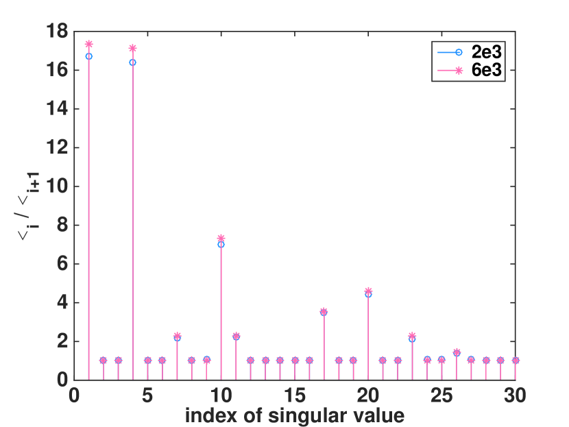
(a) $d=3$, $\exp(-\left\lVert\mathbf{x}-\mathbf{y}\right\rVert_{2}^{2}/h^{2})$

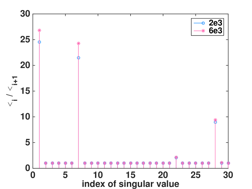
(b) $d=6$, $\exp(-\left\lVert\mathbf{x}-\mathbf{y}\right\rVert_{2}^{2}/h^{2})$

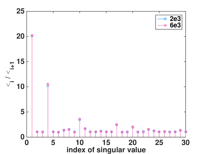
(c) $d=3$, $\frac{1}{1+\left\lVert\mathbf{x}-\mathbf{y}\right\rVert_{2}^{2}/h^{2}}$

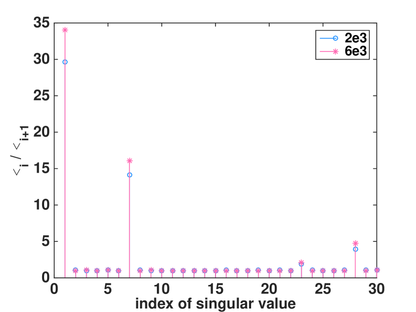
(d) $d=6$, $\frac{1}{1+\left\lVert\mathbf{x}-\mathbf{y}\right\rVert_{2}^{2}/h^{2}}$

Figure 4: Singular value ratio $\sigma_{i}/\sigma_{i+1}$ vs. index $i$. The singular values are ordered such that $\sigma_{1}\geq\sigma_{2}\geq\cdots\geq\sigma_{n}$, and the legend represents the data size (matrix dimension). Subplot (a) and (b) used Gaussian kernel $\exp(-\left\lVert\mathbf{x}-\mathbf{y}\right\rVert_{2}^{2}/h^{2})$ and subplot (c) and (d) used Cauchy kernel $1/(1+\left\lVert\mathbf{x}-\mathbf{y}\right\rVert_{2}^{2}/h^{2})$.

We study the group cardinality in detail. Consider Figure 4(a). We consider first the groups separated by significant decays. The indices with ratios above 4 are as follows with the ratio shown in parenthesis,

$$1~{}(17.3),~{}4~{}(17.1),~{}10~{}(7.3),~{}20~{}(4.5)$$

The indices can be accurately described as the cumulative sum of the number of separate terms in the following Taylor expansion terms from the first-order Fourier term,

$$\underbrace{0th}_{\text{1 term}},~{}\underbrace{1st}_{\text{3 terms}},~{}\underbrace{2nd}_{\text{6 terms}},~{}\underbrace{3rd}_{\text{10 terms}}$$

This term arrangement suggests that the polynomial approximation for the first-order Fourier term contributes to the significant gains in accuracy. We note that the higher-order Fourier terms contribute as well, but with fewer accuracy gains.

We consider next the groups separated by less significant decays. The indices with ratios above 2 are

$$1~{}(17.3),~{}4~{}(17.1),~{}7~{}(2.3),~{}10~{}(7.3),~{}11~{}(2.3),~{}17~{}(3.5),~{}20~{}(4.6)$$

These subtler gains in accuracy may come from the contributions of other higher-order expansion terms. One possible grouping is as follows, with the Fourier order and the Taylor order shown in order in parenthesis,

$$\underbrace{(1,0)}_{\text{1 term}},~{}\underbrace{(2,0),(3,0),(4,0)}_{\text{3 terms}},~{}\underbrace{(1,1)}_{\text{3 terms}},~{}\underbrace{(2,1)}_{\text{3 terms}},~{}\underbrace{(5,0)}_{\text{1 term}},~{}\underbrace{(1,2)}_{\text{6 terms}},~{}\underbrace{(3,1)}_{\text{3 terms}}$$

Applying a cumulative sum of the number of these terms yields the above indices.

Our explanation adopts the idea of the Fourier-Taylor approach instead of the Chebyshev approach. The key reason is that the Fourier approach allows us to group separate terms into finer sets that contribute to subtler error decays. The Chebyshev approach considers $\left\lVert\mathbf{x}-\mathbf{y}\right\rVert^{2l}$ as a unit, which has $\binom{l+d+1}{d+1}$ separate terms; whereas the Fourier approach considers $\left({\bm{\rho}}_{\mathbf{x}}^{T}{\bm{\rho}}_{\mathbf{y}}\right)^{l}$ as a unit, which only involves $\binom{l+d-1}{d-1}$ separate terms.

6.2 Practical Guidance

The group pattern in the singular values offers insights to many phenomena in practice. One example is the threshold matrix ranks in matrix approximations, namely the input matrix rank has to increase beyond some threshold to observe a further decay in the matrix approximation error. In practice, our quantification for the group cardinalities can provide candidate matrix rank inputs for algorithms that take input as a request matrix rank.

We examine the effectiveness of our guidance on two popular RBF kernel matrices with different low-rank algorithms. We expect significant decays in the reconstruction error around matrix rank $R=\binom{n+d}{d}$. For the leverage-score Nyström method, we oversample 30 and 60 columns for $d=6$ and $d=8$, respectively, and report the mean of reconstruction error out of 5 independent runs. Figure 5 shows the reconstruction error as a function of the approximation matrix rank. For all the algorithms, a significant decay in error occurs at rank 1, 7, and 28 for $d=6$, and at rank 1, 9 and 45 for $d=8$, in perfect agreements with our expectation. Note there exist several subtle perturbations, and they may be caused by the data layouts and contributions from other expansion terms.

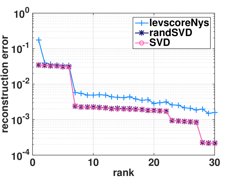
(a) $d=6$, $\exp(-\left\lVert\mathbf{x}-\mathbf{y}\right\rVert_{2}^{2}/h^{2})$

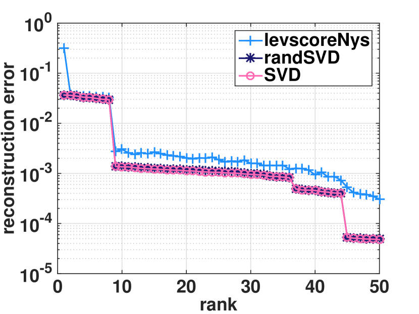
(b) $d=8$, $\exp(-\left\lVert\mathbf{x}-\mathbf{y}\right\rVert_{2}^{2}/h^{2})$

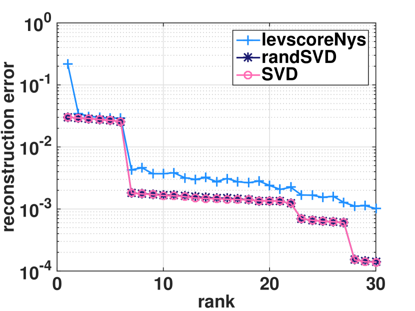
(c) $d=6$, $\frac{1}{1+\left\lVert\mathbf{x}-\mathbf{y}\right\rVert_{2}^{2}/h^{2}}$

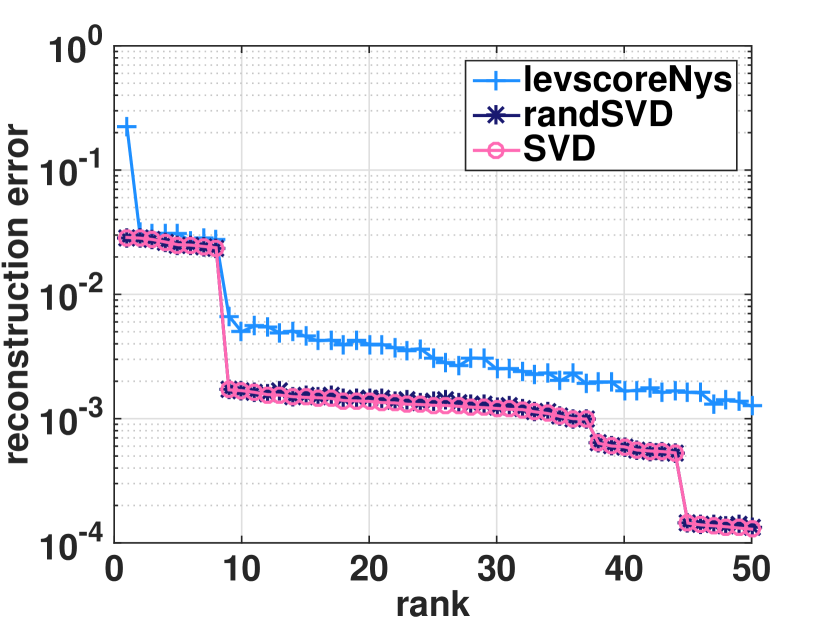
(d) $d=8$, $\frac{1}{1+\left\lVert\mathbf{x}-\mathbf{y}\right\rVert_{2}^{2}/h^{2}}$

Figure 5: Reconstruction error vs. approximation rank. The legend represents low-rank algorithms, “levscoreNys” is the leverage-score Nyström method, “randSVD” is the randomized SVD with iteration parameter to be 2, and “SVD” is the exact SVD. The bandwidth parameter $h$ was set to be the maximum pairwise distance. A significant decay in error occurs at rank = $\binom{n+d}{d}$ ($n=1,2,3$) for all experiments.

7 Conclusions

Motivated by the practical success of low-rank algorithms for RBF kernel matrices with high-dimensional datasets, we study the matrix rank of RBF kernel matrices by analyzing its upper bound, that is, the function rank of RBF kernels. Specifically, we approximate the RBF kernel by a finite sum of separate products, and quantify the upper bounds on the function ranks and the $L_{\infty}$ error for such approximations in their explicit formats. Our three main results are as follows.

First, for a fixed precision, the function rank of an RBF is a power of data dimension $d$ in the worst case, and the power is related to the precision. The exponential growth for multivariate functions from a simple analysis is absent for RBFs.

Second, for a fixed function rank, the approximation error will be reduced when the diameters of either the target domain or the source domain decrease.

Third, we observed group patterns in the magnitude of singular values of RBF kernel matrices. We explained this by our analytic expansion of the kernel function. Specifically, the number of singular values of the same magnitude can be computed by an appropriate grouping of the separate terms in the function’s separable form. Very commonly, the cardinality of the $i$-th group is $\binom{i+d-1}{d-1}$.

References

- [1] K. Ball, N. Sivakumar, and J. D. Ward, On the sensitivity of radial basis interpolation to minimal data separation distance, Constructive Approximation, 8 (1992), pp. 401–426.
- [2] V. Barthelmann, E. Novak, and K. Ritter, High dimensional polynomial interpolation on sparse grids, Adv. Comput. Math., 12 (2000), pp. 273–288.
- [3] P. S. Bernstein, Sur les recherches recentes relatives a la meilleure approximation des fonctions con-tinues par des polynômes, (1912).
- [4] S. Bernstein, Probability theory, moscow-leningrad, 1946.
- [5] J. P. Boyd, A comparison of numerical algorithms for Fourier extension of the first, second, and third kinds, J. Comput. Phys., 178 (2002), pp. 118–160.
- [6] C. Cortes and V. Vapnik, Support-vector networks, Mach. Learn., 20 (1995), pp. 273–297.
- [7] N. Cristianini and J. Shawe-Taylor, An introduction to support vector machines: And other kernel-based learning methods, Cambridge University Press, New York, NY, USA, 2000.
- [8] P. Drineas, M. Magdon-Ismail, M. W. Mahoney, and D. P. Woodruff, Fast approximation of matrix coherence and statistical leverage, J. Mach. Learn. Res., 13 (2012), pp. 3475–3506.
- [9] P. Drineas and M. W. Mahoney, On the Nyström method for approximating a Gram matrix for improved kernel-based learning, J. Mach. Learn. Res., 6 (2005), pp. 2153–2175.
- [10] T. A. Driscoll and B. Fornberg, Interpolation in the limit of increasingly flat radial basis functions, Computers & Mathematics with Applications, 43 (2002), pp. 413–422.
- [11] N. El Karoui, The spectrum of kernel random matrices, Ann. Stat., 38 (2010), pp. 1–50.
- [12] B. Fornberg, E. Larsson, and N. Flyer, Stable computations with Gaussian radial basis functions, SIAM J. Sci. Comput., 33 (2011), pp. 869–892.
- [13] B. Fornberg, G. Wright, and E. Larsson, Some observations regarding interpolants in the limit of flat radial basis functions, Computers & mathematics with applications, 47 (2004), pp. 37–55.
- [14] B. Fornberg and J. Zuev, The Runge phenomenon and spatially variable shape parameters in RBF interpolation, Comput. Math. with Appl., 54 (2007), pp. 379–398.
- [15] T. Gerstner and M. Griebel, Numerical integration using sparse grids, Numer. Algorithms, 18 (1998), pp. 209–232.
- [16] C. R. Giardina and P. M. Chirlian, Bounds on the truncation error of periodic signals, IEEE Trans. Circuit Theory, 19 (1972), pp. 206–207.
- [17] A. Gittens and M. W. Mahoney, Revisiting the Nyström method for improved large-scale machine learning, J. Mach. Learn. Res., 17 (2016), pp. 3977–4041.
- [18] G. H. Golub and C. F. Van Loan, Matrix Computations, The Johns Hopkins University Press, 4th ed., 2013.
- [19] N. Halko, P.-G. Martinsson, and J. A. Tropp, Finding structure with randomness: probabilistic algorithms for constructing approximate matrix decompositions, SIAM Rev., 53 (2011), pp. 217–288.
- [20] T. Hofmann, B. Schölkopf, and A. J. Smola, Kernel methods in machine learning, Ann. Stat., 36 (2008), pp. 1171–1220.
- [21] P. K. Kitanidis, Compressed state Kalman filter for large systems, Adv. Water Resour., 76 (2015), pp. 120–126.
- [22] J. Y. Li, S. Ambikasaran, E. F. Darve, and P. K. Kitanidis, A Kalman filter powered by H2-matrices for quasi-continuous data assimilation problems, Water Resour. Res., 50 (2014), pp. 3734–3749.
- [23] E. Liberty, F. Woolfe, P.-G. Martinsson, V. Rokhlin, and M. Tygert, Randomized algorithms for the low-rank approximation of matrices, Proc. Natl. Acad. Sci. U. S. A., 104 (2007), pp. 20167–72.
- [24] G. Little and J. Reade, Eigenvalues of analytic kernels, SIAM journal on mathematical analysis, 15 (1984), pp. 133–136.
- [25] M. W. Mahoney, Randomized algorithms for matrices and data, Found. Trends® Mach. Learn., 3 (2011), pp. 123–224.
- [26] C. A. Micchelli, Interpolation of scattered data: distance matrices and conditionally positive definite functions, in Approximation theory and spline functions, Springer, 1984, pp. 143–145.
- [27] F. J. Narcowich and J. D. Ward, Norm estimates for the inverses of a general class of scattered-data radial-function interpolation matrices, J. Approx. Theory, 69 (1992), pp. 84–109.
- [28] E. Novak and K. Ritter, Simple cubature formulas with high polynomial exactness, Constr. Approx., 15 (1999), pp. 499–522.
- [29] C. E. Rasmussen and C. K. I. Williams, Gaussian processes for machine learning, The MIT Press, 2005.
- [30] T. Sarlos, Improved approximation algorithms for large matrices via random projections, in Proc. 47th Annu. IEEE Symp. Found. Comput. Sci., IEEE, 2006, pp. 143–152.
- [31] R. Schaback, Lower bounds for norms of inverses of interpolation matrices for radial basis functions, J. Approx. Theory, 79 (1994), pp. 287–306.
- [32] , Error estimates and condition numbers for radial basis function interpolation, Adv. Comput. Math., 3 (1995), pp. 251–264.
- [33] , Limit problems for interpolation by analytic radial basis functions, Journal of Computational and Applied Mathematics, 212 (2008), pp. 127–149.
- [34] B. Schölkopf and A. J. Smola, Learning with kernels: support vector machines, regularization, optimization, and beyond, MIT Press, 2002.
- [35] S. A. Smolyak, Quadrature and interpolation formulas for tensor products of certain classes of functions, in Sov. Math. Dokl., vol. 4, 1963, pp. 240–243.
- [36] L. N. Trefethen, Approximation theory and approximation practice, Society for Industrial and Applied Mathematics, Philadelphia, PA, USA, 2013.
- [37] , Cubature, approximation, and isotropy in the hypercube, SIAM Rev. to Appear, (2016).
- [38] V. N. Vapnik, Statistical learning theory, Wiley, 1998.
- [39] R. Wang, Y. Li, M. W. Mahoney, and E. Darve, Structured block basis factorization for scalable kernel matrix evaluation, tech. rep., 2015.
- [40] A. J. Wathen and S. Zhu, On spectral distribution of kernel matrices related to radial basis functions, Numer. Algorithms, 70 (2015), pp. 709–726.
- [41] H. Wendland, Scattered data approximation, vol. 17, Cambridge university press, 2004.
- [42] H. Woźniakowski, Tractability and strong tractability of linear multivariate problems, J. Complex., 10 (1994), pp. 96–128.
- [43] K. Zhang and J. T. Kwok, Clustered Nyström method for large scale manifold learning and dimension reduction, IEEE Trans. Neural Networks, 21 (2010), pp. 1576–1587.
- [44] B. Zwicknagl, Power series kernels, Constructive Approximation, 29 (2009), pp. 61–84.