Second-Order Moment-Closure for Tighter Epidemic Thresholds

Abstract

In this paper, we study the dynamics of contagious spreading processes taking place in complex contact networks. We specifically present a lower-bound on the decay rate of the number of nodes infected by a susceptible-infected-susceptible (SIS) stochastic spreading process. A precise quantification of this decay rate is crucial for designing efficient strategies to contain epidemic outbreaks. However, existing lower-bounds on the decay rate based on first-order mean-field approximations are often accompanied by a large error resulting in inefficient containment strategies. To overcome this deficiency, we derive a lower-bound based on a second-order moment-closure of the stochastic SIS processes. The proposed second-order bound is theoretically guaranteed to be tighter than existing first-order bounds. We also present various numerical simulations to illustrate how our lower-bound drastically improves the performance of existing first-order lower-bounds in practical scenarios, resulting in more efficient strategies for epidemic containment.

1 Introduction

Understanding the dynamics of spreading processes taking place in complex networks is one of the central questions in the field of network science, with applications in information propagation in social networks [1], epidemiology [2], and cyber-security [3]. Among various quantities characterizing the asymptotic behaviors of spreading processes, the decay rate (see, e.g., [4, 5]) of the spreading size (i.e., the number of nodes affected by the spread) is of fundamental importance. Besides quantifying the impact of contagious spreading processes over networks [6, 7], the decay rate has been used to measure the performance of containment strategies to control epidemic outbreaks [8]. In this direction, the authors in [9] presented an optimization-based approach for distributing a limited amount of resources to efficiently contain spreading processes by maximizing their decay rate towards the disease-free equilibrium. This framework was later extended to the cases where the underlying network in which the spreading process is taking place is uncertain [10], temporal [11, 12], and adaptively changing [13, 14]. Recently, the authors in [15] presented an approach for achieving an optimal resource allocation in order to maximize the decay rate under sparsity constraints.

However, finding the decay rate of a spreading process is, in general, a computationally hard problem. Even for the case of the susceptible-infected-susceptible (SIS) model [2], which is one of the simplest models of spread, the exact decay rate is given in terms of the eigenvalues of a matrix whose size grows exponentially fast with respect to the number of nodes in the networks [4]. In order to avoid this computational difficulty, it is common in the literature [9, 10, 15] to use a lower-bound on the decay rate based on first-order mean-field approximations of the spreading processes. However, this first-order approximation is not necessarily accurate; in other words, its approximation error can be significantly large for several important social and biological networks, as we will demonstrate later in this paper. Therefore, the design of strategies for epidemic containment based on mean-field approximations can result in inefficient control policies.

The aim of this paper is to present a tighter lower-bound on the decay rate of the stochastic SIS process based on a second-order moment closure. Specifically, we show that the decay rate is bounded from below by the maximum real eigenvalue of a Metzler matrix whose size grows quadratically with respect to the number of nodes in the network. In order to derive our lower-bound, we describe the stochastic dynamics of the SIS process using a system of stochastic differential equations with Poisson jumps. This approach allows us to conveniently evaluate the dynamics of the first and the second-order moments of random variables relevant for the spreading processes. Furthermore, we prove theoretically and illustrate numerically that our lower-bound strictly improves the one based on first-order approximations.

We remark that, although improved decay rates for the discrete-time SIS model were presented using second-order analysis in [16], their bounds are applicable only to the special case where the transmission and recovery rates of nodes are homogeneous and, furthermore, satisfy restrictive algebraic conditions in terms of nonnegativity of infinitely many matrices. Likewise, the second-order analysis of the continuous-time SIS model by the authors in [17] uses mean-field approximations and, hence, it is not clear how the analysis relates to the dynamics of the original stochastic SIS process. Moreover, their analysis is valid only when a dominant eigenvalue of a certain matrix (i.e., an eigenvalue having the maximum real part) is real. In contrast with these limitations of the results in the literature, our framework applies to the heterogeneous SIS model without any restrictions, and is supported by rigorous proofs instead of approximations.

This paper is organized as follows. In Section 2, we state the problem studied in this paper. In Section 3, we present our lower-bound on the decay rate, and show that this bound strictly improves the one based on first-order approximations. The effectiveness of our lower-bound is numerically illustrated in Section 4.

1.1 Mathematical preliminaries

We denote the identity and the zero matrices by $I$ and $O$, respectively. For a vector $u$, we denote by $u_{\backslash\{i\}}$ the vector that is obtained after removing the $i$th element from $u$. Likewise, for a matrix $A$, we let $A_{i,\backslash\{j\}}$ denote the row vector that is obtained after removing the $j$th element from the $i$th row of $A$. We say that a square matrix $A$ is irreducible if no similarity transformation by a permutation matrix transforms $A$ into a block upper-triangular matrix. The block-diagonal matrix containing matrices $A_{1}$, $\dotsc$, $A_{n}$ as its diagonal blocks is denoted by $\bigoplus_{i=1}^{n}A_{i}$. If the matrices $A_{1}$, $\dotsc$, $A_{n}$ have the same number of columns, then the matrix obtained by stacking $A_{1}$, $\dotsc$, $A_{n}$ in vertical is denoted by $\operatorname*{col}_{1\leq i\leq n}A_{i}$.

A directed graph is defined as the pair $\mathcal{G}=(\mathcal{V},\mathcal{E})$, where $\mathcal{V}$ is a finite ordered set of nodes and $\mathcal{E}\subset\mathcal{V}\times\mathcal{V}$ is a set of directed edges. By convention, if $(v,v^{\prime})\in\mathcal{E}$, we understand that there is an edge from $v$ pointing towards $v^{\prime}$, in which case $v$ is said to be an in-neighbor of $v^{\prime}$. A directed path from $v$ to $v^{\prime}$ in $\mathcal{G}$ is an ordered set of nodes $(v_{0},\dotsc,v_{\ell})$ such that $v_{0}=v$, $v_{\ell}=v^{\prime}$, and $(v_{{k}},v_{k+1})\in\mathcal{E}$ for $k=0,\dotsc,\ell-1$. We say that $\mathcal{G}$ is strongly connected if there exists a directed path from $v$ to $v^{\prime}$ for all $v,v^{\prime}\in\mathcal{V}$. The adjacency matrix of $\mathcal{G}$ is defined as the square matrix, having the same dimension as the number of the nodes, such that its $(i,j)$th entry equals $1$ if the $j$th node is an in-neighbor of the $i$th node, and equals $0$ otherwise. It is well known that a directed graph is strongly connected if and only if its adjacency matrix is irreducible.

A real matrix $A$ (or a vector as its special case) is said to be nonnegative, denoted by $A\geq 0$, if all the entries of $A$ are nonnegative. Likewise, if all the entries of $A$ are positive, then $A$ is said to be positive. For another matrix $B$ having the same dimensions as $A$, the notation $A\leq B$ implies $B-A\geq 0$. If $A\leq B$ and $A\neq B$, we write $A\lneq B$. For a square matrix $A$, we say that $A$ is Metzler [18] if the off-diagonal entries of $A$ are nonnegative. It is easy to see that $e^{At}\geq 0$ if $A$ is Metzler and $t\geq 0$ (see, e.g., [18]). For a Metzler matrix $A$, the maximum real part of the eigenvalues of $A$ is denoted by $\lambda_{\max}(A)$. In this paper, we use the following basic properties of Metzler matrices:

Lemma 1.

The following statements hold for a Metzler matrix $A$:

1. $\lambda_{\max}(A)$ is an eigenvalue of $A$. Moreover, if $A$ is irreducible, then there exists a positive eigenvector corresponding to the eigenvalue $\lambda_{\max}(A)$.

2. If $A\leq B$, then $\lambda_{\max}(A)\leq\lambda_{\max}(B)$. Furthermore, if $A$ is irreducible and $A\neq B$, then $\lambda_{\max}(A)<\lambda_{\max}(B)$.

3. Assume that $A$ is irreducible. If there exist a positive vector $u$ and a positive constant $\rho$ such that $Au\lneq\rho u$, then $\lambda_{\max}(A)<\rho$.

Proof.

The first claim is part of the Perron-Frobenius theorem for Metzler matrices (see, e.g., [18, Theorems 11 and 17]). The second claim follows from the Perron-Frobenius theory and the monotonicity of the maximum real eigenvalue of nonnegative matrices [19, Section 8.4]. To prove the last statement, let $\epsilon=\rho u-Au$ and define $A^{\prime}=A+\bigoplus(\epsilon_{1}/u_{1},\dotsc,\epsilon_{n}/u_{n})$, where $n$ is the length of the vector $u$. Since $A^{\prime}u=Au+\epsilon=\rho u$, $A^{\prime}$ is irreducible, and $v$ is positive, it follows that $\lambda_{\max}(A^{\prime})=\rho$ from the Perron-Frobenius theorem for irreducible Metzler matrices [18, Theorem 17]. Since $A$ is irreducible and $A\lneq A^{\prime}$, the second statement of the lemma shows that $\lambda_{\max}(A)<\lambda_{\max}(A^{\prime})=\rho$. ∎

2 Problem Statement

We start by giving a brief overview of the SIS model [2]. Let $\mathcal{G}=(\mathcal{V},\mathcal{E})$ be a strongly connected directed graph with nodes $v_{1}$, $\dotsc$, $v_{n}$. In the SIS model, at a given (continuous) time $t\geq 0$, each node can be in one of two possible states: susceptible or infected. When a node $v_{i}$ is infected, it can randomly transition to the susceptible state with an instantaneous rate $\delta_{i}>0$, called the recovery rate of node $v_{i}$. On the other hand, if an in-neighbor of node $v_{i}$ is in the infected state, then the in-neighbor can infect node $v_{i}$ with an instantaneous rate $\beta_{i}$, where $\beta_{i}>0$ is called the infection rate of node $v_{i}$. It is easy to see that the SIS model is a continuous-time Markov process and has a unique absorbing state at which all the nodes are susceptible. Since this absorbing state is reachable from any other state, the SIS model reaches this infection-free absorbing state in a finite time with probability one. The aim of this paper is to study the stability of this infection-free absorbing state, defined as follows:

Definition 2.

Let $\epsilon>0$ and define the probability

$$p_{i}(t)=\operatorname{Pr}(\text{$v_{i}$ is infected at time $t$}).$$

We say that the SIS model is $\epsilon$-exponentially mean stable if there exists a constant $C>0$ such that, for all nodes $v_{i}$ and $t\geq 0$, we have $p_{i}(t)\leq Ce^{-\epsilon t}$ for any set of initially infected nodes at time $t=0$. Then, we define the decay rate of the SIS model as $\rho=\sup\{\epsilon\colon\text{SIS model is $\epsilon$-exponentially stable}\}$.

The notion of the decay rate was studied in, e.g., [4] and [5] for the cases of continuous- and discrete-time problem settings, respectively, and is closely related to other important quantities on spreading processes such as epidemic thresholds [4] and mean-time-to-absorption [7]. Specifically, a basic argument from the theory of Markov processes shows that the SIS model is $\epsilon$-exponentially mean stable for a sufficiently small $\epsilon>0$ (with a possibly large $C$) and, therefore, it always has a positive decay rate. However, exact computation of the decay rate is hard in practice. Even in the homogeneous case, where all nodes share the same infection and recovery rates, the decay rate equals the modulus of the largest real-part of the non-zero eigenvalues of a $2^{n}\times 2^{n}$ matrix representing the infinitesimal generator of the SIS model [4]. An alternative approach for analyzing the decay rate is via upper bounds on the dynamics of the SIS model based on first-order mean-field approximations. An example of such a first-order upper bound is described below. Let us define the vector $p(t)=\operatorname*{col}_{1\leq i\leq n}p_{i}(t)$ containing the infection probabilities of the nodes. Also, let $A$ be the adjacency matrix of $\mathcal{G}$ and define the diagonal matrices $B=\bigoplus(\beta_{1},\dotsc,\beta_{n})$ and $D=\bigoplus(\delta_{1},\dotsc,\delta_{n})$. Then, we can show [9] the inequality $p(t)\leq e^{(BA-D)t}p(0)$, which gives the following lower-bound on the decay rate:

$$\rho\geq\rho_{1}=-\lambda_{\max}(BA-D).$$ (1)

Although this lower-bound is computationally efficient to find, there are several cases in which we can observe a large gap between this bound and the exact decay rate, as illustrated in the following example:

Example 3.

Let us consider the SIS model over a romantic and sexual network in a high school (Jefferson, $n=288$) taken from [20]. For simplicity, we assume a homogeneous transmission rate $\beta_{i}=0.9/\lambda_{\max}(A)$ and a (normalized) recovery rate $\delta_{i}=1$ for all nodes. In order to approximately compute the true decay rate $\rho$, we generate $10,000$ sample paths of the SIS model over the time interval $[0,100]$ starting from the initial state at which all nodes are infected. From this computation, we obtain a decay rate of $\rho\approx 0.454$. On the other hand, the first-order approximation in (1) equals $\rho_{1}=0.1$, whose relative error from $\rho$ is around 78%.

Remark 4.

We can in fact show that the strict inequality $\rho>\rho_{1}$ holds in (1). Let $v_{i}$ be a node having the minimum recovery rate $\delta_{\min}=\min_{1\leq i\leq n}\delta_{i}>0$ among all nodes, and consider the situation where only the node $v_{i}$ is initially infected. Since $p_{i}(t)\geq e^{-\delta_{i}t}$ for every $t\geq 0$, we have

$$\rho\geq\delta_{i}=\delta_{\min}.$$ (2)

Then, let us take an arbitrary positive constant $b<\min_{1\leq i\leq n}\beta_{i}$. Since $\delta_{\min}=-\lambda_{\max}(-D)$ and $-D\leq bA-D$, Lemma 1.2 shows

$$-\delta_{\min}\leq\lambda_{\max}(bA-D).$$ (3)

On the other hand, Since $bA-D$ is irreducible (by the strong connectivity of $\mathcal{G}$) and $bA-D\lneq BA-D$, we also have

$$\lambda_{\max}(bA-D)<\lambda_{\max}(BA-D)=-\rho_{1}$$ (4)

by Lemma 1.2. Inequalities (2)–(4) prove the strict inequality $\rho>\rho_{1}$, as desired.

3 Main Result

As we have demonstrated in Example 3, there may be a large gap between the true decay rate $\rho$ and its first-order approximation $\rho_{1}$ for the SIS model. The aim of this paper is to fill in this gap by providing a better lower-bound on the decay rate. Specifically, the following theorem presents an improved lower-bound on the decay rate and is the main result of this paper:

Theorem 5.

Define the $n^{2}\times n^{2}$ Metzler matrix

$$\mathcal{A}\!=\!\begin{bmatrix}-D&\bigoplus_{i=1}^{n}(\beta_{i}A_{i,\backslash\{i\}})\\ \operatorname*{col}_{1\leq i\leq n}(\delta_{i}V_{i})&\ \ \bigoplus_{i=1}^{n}\left(-\Gamma_{i}+\operatorname*{col}_{j\neq i}\beta_{j}A_{j,\backslash\{i\}}\right)\end{bmatrix},$$

where $V_{i}\in\mathbb{R}^{(n-1)\times n}$ is the matrix satisfying $V_{i}x=x_{\backslash\{i\}}$ for all $x\in\mathbb{R}^{n}$, and $\Gamma_{i}=\bigoplus_{j\neq i}\gamma_{ij}$ for $\gamma_{ij}=\delta_{i}+\delta_{j}+a_{ij}\beta_{i}$. Define $\rho_{2}=-\lambda_{\max}(\mathcal{A})$. Then, we have

$$\rho\geq\rho_{2}>\rho_{1}.$$

In order to prove this theorem, we use a representation of the SIS model as a system of stochastic differential equations with Poisson jumps (see, e.g., [13]). For this purpose, we define the variable $x_{i}(t)$ as $x_{i}(t)=1$ if node $v_{i}$ is infected at time $t$, and $x_{i}(t)=0$ otherwise. Then, we can see that these variables obey the following stochastic differential equations with Poisson jumps:

$$dx_{i}=-x_{i}dN_{\delta_{i}}+\sum_{k=1}^{n}a_{ik}(1-x_{i})x_{k}dN_{\beta_{i}},$$ (5)

where $a_{ik}$ is the $(i,k)$th entry of the adjacency matrix and $N_{\delta_{i}}$ and $N_{\beta_{i}}$ denote stochastically independent Poisson counters [21, Chapter 1] with rates $\delta_{i}$ and $\beta_{i}$, respectively. The rest of this section is devoted to the proof of the theorem. We divide the proof into two parts, namely, the proof of $\rho\geq\rho_{2}$ (Subsection 3.1) and $\rho_{2}>\rho_{1}$ (Subsection 3.2).

3.1 Proof of $\rho\geq\rho_{2}$

From the system (5) of stochastic differential equations, we can easily show [13] that the expectation $p_{i}=E[x_{i}]$ obeys the differential equation

$$\frac{dp_{i}}{dt} =-\delta_{i}E[x_{i}]+\sum_{k=1}^{n}a_{ik}E[(1-x_{i})x_{k}]\beta_{i}$$

$$=-\delta_{i}p_{i}+\beta_{i}\sum_{k\neq i}a_{ik}q_{ik},$$ (6)

where $q_{ij}(t)=E[(1-x_{i}(t))x_{j}(t)]$ is a second-order variable representing the probability that $v_{i}$ is susceptible and $v_{j}$ is infected at time $t$. Since $q_{ii}\equiv 0$ by definition, in the sequel we do not consider the variable of the form $q_{ii}$. We next derive differential equations to characterize the second-order variables $q_{ij}$. Applying Ito’s formula (see, e.g., [21, Chapter 4]) for stochastic differential equations with Poisson jumps to the variable $(1-x_{i})x_{j}$, we can show

$$d((1-x_{i})x_{j}) =x_{i}x_{j}dN_{\delta_{j}}-(1-x_{i})x_{j}\sum_{k=1}^{n}a_{ik}x_{k}dN_{\beta_{i}}$$ (7)

$$\quad-(1-x_{i})x_{j}dN_{\delta_{j}}+(1-x_{i})(1-x_{j})\sum_{k=1}^{n}a_{jk}x_{k}dN_{\beta_{j}}$$

for any distinct pair $(v_{i},v_{j})$ of nodes. To proceed, we define the probabilities $p_{ij}(t)=E[x_{i}(t)x_{j}(t)]$ and $p_{ijk}(t)=E[x_{i}(t)x_{j}(t)x_{k}(t)]$ for nodes $v_{i}$, $v_{j}$, and $v_{k}$. Then, from (7), we can compute the derivative of $q_{ij}$ as

$$\frac{dq_{ij}}{dt} =\delta_{j}E[x_{i}x_{j}]-\beta_{i}\sum_{k=1}^{n}a_{ik}E[(1-x_{i})x_{j}x_{k}]$$

$$\quad-\delta_{j}E[(1\!-\!x_{i})x_{j}]+\beta_{j}\sum_{k=1}^{n}a_{jk}E[(1\!-\!x_{i})(1\!-\!x_{j})x_{k}]$$

$$=\delta_{i}p_{ij}-\beta_{i}a_{ij}(p_{j}-p_{ij})-\delta_{j}q_{ij}+\beta_{j}\sum_{k=1}^{n}a_{jk}(p_{k}-p_{ik})-\epsilon_{ij},$$

where the function $\epsilon_{ij}=\beta_{i}\sum_{k\neq j}a_{ik}(p_{jk}-p_{ijk})+\beta_{j}\sum_{k=1}^{n}a_{jk}(p_{jk}-p_{ijk})$ is nonnegative because $p_{jk}\geq p_{ijk}$ for all nodes $v_{i}$, $v_{j}$, and $v_{k}$. Using the identity $p_{j}-p_{ij}=q_{ij}$ and defining the variable $\gamma_{ij}=\delta_{i}+\delta_{j}+a_{ij}\beta_{i}$, we obtain

$$\frac{dq_{ij}}{dt}=-\gamma_{ij}q_{ij}+\delta_{i}p_{j}+\beta_{j}\sum_{k\neq i}a_{jk}q_{ik}-\epsilon_{ij}.$$ (8)

In order to upper-bound the infection probabilities of the nodes, we define the vector variables $q_{i}=\operatorname*{col}_{j\neq i}q_{ij}$ and $q=\operatorname*{col}_{1\leq i\leq n}q_{i}$ having dimensions $n-1$ and $n(n-1)$, respectively. Then, we can rewrite the differential equation (6) as ${dp_{i}}/{dt}=-\delta_{i}p_{i}+\beta_{i}A_{i,\backslash\{i\}}q_{i}$. Stacking this differential equation in vertical with respect to $i$, we obtain

$$\frac{dp}{dt}=-Dp+\biggl{(}\bigoplus_{1=1}^{n}\beta_{i}A_{i,\backslash\{i\}}\biggr{)}q,$$ (9)

where $D=\bigoplus(\delta_{1},\dotsc,\delta_{n})$. Also, from (8), it follows that ${dq_{ij}}/{dt}=-\gamma_{ij}q_{ij}+\delta_{i}p_{j}+\beta_{j}A_{j,\backslash\{i\}}q_{i}-\epsilon_{ij}$. Stacking this differential equation with respect to $j\in\{1,\dotsc,n\}\backslash\{i\}$, we see that

$$\frac{dq_{i}}{dt}=-\Gamma_{i}q_{i}+\delta_{i}V_{i}p+\left(\operatorname*{col}_{j\neq i}(\beta_{j}A_{j,\backslash\{i\}})\right)q_{i}-\operatorname*{col}_{j\neq i}\epsilon_{ij}.$$

By stacking this differential equation with respect to $i=1,\dotsc,n$, we obtain the following differential equation

$$\frac{dq}{dt}=\left(\operatorname*{col}_{1\leq i\leq n}\delta_{i}V_{i}\right)p+\bigoplus_{i=1}^{n}\left(-\Gamma_{i}+\operatorname*{col}_{j\neq i}\beta_{j}A_{j,\backslash\{i\}}\right)q-\epsilon,$$

where $\epsilon=\operatorname*{col}_{1\leq i\leq n}\operatorname*{col}_{j\neq i}\epsilon_{ij}$ is a vector-valued nonnegative function. This differential equation and (9) show that the variable $r=\operatorname*{col}(p,q)$ satisfies $dr/dt=\mathcal{A}r-\operatorname*{col}(0,\epsilon)$.

We are now at the position to prove the inequality $\rho\geq\rho_{2}$. Since $\mathcal{A}$ is Metzler and $\epsilon(t)$ is entry-wise nonnegative for every $t\geq 0$, we can obtain the upper bound $r(t)=e^{\mathcal{A}t}r(0)-\int_{0}^{t}e^{\mathcal{A}(t-\tau)}\operatorname*{col}(0,\epsilon(\tau))\,d\tau\leq e^{\mathcal{A}t}r(0)$. This inequality clearly implies that the SIS model is $\rho_{2}$-exponentially mean stable. This completes the proof of the inequality.

3.2 Proof of $\rho_{2}>\rho_{1}$

If $\rho_{2}\geq\delta_{\min}$, then we trivially have $\rho_{2}>\rho_{1}$ because we know $\delta_{\min}>\rho_{1}$ from (3) and (4). Let us consider the case of $\rho_{2}<\delta_{\min}$. Let $u$ be a non-zero vector of $\mathcal{A}$ corresponding to the eigenvalue $-\rho_{2}=\lambda_{\max}(\mathcal{A})$, i.e., assume that $\mathcal{A}u=-\rho_{2}u$. We split the matrix $\mathcal{A}$ as $\mathcal{A}=\mathcal{M}-\mathcal{N}$ using the matrices

$$\mathcal{M}=\begin{bmatrix}O&\mathcal{M}_{12}\\ O&\mathcal{M}_{22}\end{bmatrix},\ \mathcal{N}=\begin{bmatrix}D&O\\ \mathcal{N}_{21}&\mathcal{N}_{22}\end{bmatrix},$$

where

$$\begin{gathered}\mathcal{M}_{12}=\bigoplus_{i=1}^{n}\beta_{i}A_{i,\backslash\{i\}},\ \mathcal{M}_{22}=\bigoplus_{i=1}^{n}\left(\operatorname*{col}_{j\neq i}(\beta_{j}A_{j,\backslash\{i\}})-\bigoplus_{j\neq i}a_{ij}\beta_{i}\right),\\ \mathcal{N}_{21}=-\operatorname*{col}_{1\leq i\leq n}\delta_{i}V_{i},\ \mathcal{N}_{22}=\bigoplus_{i=1}^{n}\bigoplus_{j\neq i}(\delta_{i}+\delta_{j}).\end{gathered}$$

Then, we have $\mathcal{M}u=(\mathcal{N}-\rho_{2}I)u$ and, hence, $(\mathcal{N}-\rho_{2}I)^{-1}\mathcal{M}u=u$, where the inversion of $\mathcal{N}-\rho_{2}I$ is allowed by our assumption $\rho_{2}<\delta_{\min}$. Therefore, the matrix $(\mathcal{N}-\rho_{2}I)^{-1}\mathcal{M}$ has an eigenvalue equal to $1$. Since this matrix has the following upper-triangular structure

$$(\mathcal{N}-\rho_{2}I)^{-1}\mathcal{M}=\begin{bmatrix}O&*\\ O&\mathcal{L}\end{bmatrix}$$

for the Metzler matrix $\mathcal{L}$ defined by

$$\mathcal{L}=(\mathcal{N}_{22}-\rho_{2}I)^{-1}(-\mathcal{N}_{21}(D-\rho_{2}I)^{-1}\mathcal{M}_{12}+\mathcal{M}_{22}),$$

it follows that $\mathcal{L}$ has an eigenvalue equal to $1$. This specifically implies that

$$\lambda_{\max}(\mathcal{L})\geq 1.$$ (10)

On the other hand, we can obtain an upper bound on $\lambda_{\max}(\mathcal{L})$ as follows. The irreducible matrix $BA-D$ has a positive eigenvector $v$ corresponding to the eigenvalue $-\rho_{1}$ by Lemma 1.1. Define the positive vector $w=\operatorname*{col}_{1\leq i\leq n}v_{\backslash\{i\}}$. Then, it is easy to see that $\mathcal{M}_{12}w=BAv$ and $\mathcal{M}_{22}w=\operatorname*{col}_{1\leq i\leq n}(BAv)_{\backslash\{i\}}-\operatorname*{col}_{1\leq i\leq n}\operatorname*{col}_{j\neq i}\beta_{j}a_{ij}v_{i}$. Using these equalities and the eigenvalue equation $(BA-D)v=-\rho_{1}v$, we can show that

$$\mathcal{L}w =(\mathcal{N}_{22}-\rho_{2}I)^{-1}\operatorname*{col}_{i}\left(\delta_{i}V_{i}(D-\rho_{2}I)^{-1}(D-\rho_{1}I)v\right)$$

$$\quad+(\mathcal{N}_{22}-\rho_{2}I)^{-1}\operatorname*{col}_{i}((D-\rho_{1}I)v)_{\backslash\{i\}}-\phi$$

$$=\operatorname*{col}_{i}\operatorname*{col}_{j\neq i}\left(\frac{\delta_{j}-\rho_{1}}{\delta_{j}-\rho_{2}}v_{j}\right)-\phi$$

$$\leq\left(\max_{1\leq i\leq n}\frac{\delta_{i}-\rho_{1}}{\delta_{i}-\rho_{2}}\right)w-\phi$$ (11)

for the nonzero and nonnegative vector

$$\phi=\operatorname*{col}_{1\leq i\leq n}\operatorname*{col}_{j\neq i}\frac{a_{ij}(\beta_{i}v_{j}+\beta_{j}v_{i})}{\delta_{i}+\delta_{j}-\rho_{2}}.$$

Since $\mathcal{L}$ is irreducible (for the proof, see Appendix A), the inequality (11) and Lemma 1.3 show $\lambda_{\max}(\mathcal{L})<\max_{1\leq i\leq n}(\delta_{i}-\rho_{1})/(\delta_{i}-\rho_{2})$. Since we have already shown (10), there must exist an $i$ such that $1<(\delta_{i}-\rho_{1})/(\delta_{i}-\rho_{2})$. This inequality is equivalent to $\rho_{2}>\rho_{1}$ because both of $\delta_{i}-\rho_{1}$ and $\delta_{i}-\rho_{2}$ are positive. This completes the proof.

4 Numerical Simulations

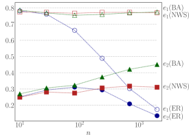
(a) $\beta=0.9/\lambda_{\max}(A)$

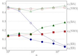
(b) $\beta=0.7/\lambda_{\max}(A)$

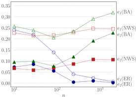
(c) $\beta=0.5/\lambda_{\max}(A)$

Figure 1: Relative approximation errors of the decay rate $\rho$ for ER (circles), BA (triangles), and NWS (squares) graphs. Empty markers: first-order bound $\rho_{1}$, filled markers: second-order bound $\rho_{2}$.

In this section, we illustrate the effectiveness of our results with numerical simulations. The simulations are performed using Python 3.6 on a 4.2 GHz Intel Core i7 processor. In our simulations, we consider the SIS model over several complex networks with a homogeneous transmission rate $\beta_{i}=\beta$ and a recovery rate $\delta_{i}=\delta$ for all nodes. We normalize $\delta=1$ without loss of generality. We first consider the following three random graphs: 1) Erdös-Rényi (ER), 2) Barabási-Albert (BA), and 3) Newman-Watts-Strogatz (NWS) graphs. For each of the networks and various network sizes, we compute the first-order bound $\rho_{1}$, our second-order bound $\rho_{2}$, and an approximation of the true decay rate $\rho$ (by the same procedure used in Example 3). We present the sample averages of the relative errors $e_{1}=(\rho-\rho_{1})/\rho$ and $e_{2}=(\rho-\rho_{2})/\rho$ in Fig. 1 (20 realizations of random graphs for each data point) for $\beta=0.9/\lambda_{\max}(A)$, $0.7/\lambda_{\max}(A)$, and $0.5/\lambda_{\max}(A)$. We can observe that our second-order bound remarkably improves the first-order bound, specifically for the cases of BA and NWS networks.

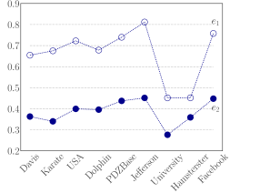
Figure 2: Relative approximation errors of the decay rate $\rho$ for real networks. Empty markers: first-order bound $\rho_{1}$, filled-markers: second-order bound $\rho_{2}$.

We then consider the SIS model over several real-world networks [22]. Specifically, we compute lower-bounds on the decay rates for 1) a bipartite network from participation of women in social events (Davis, $n=32$), 2) a social network of the Zachary’s Karate club (Karate, $n=34$), 3) the connectivity network of states in the USA (USA, $n=49$), 4) a network of bottlenose dolphins (Dolphin, $n=62$), 5) a network of protein-protein interactions (PDZBase, $n=212$), 6) the high-school network described in Example 3 (Jefferson, $n=288$), 7) an email communication network at the University Rovira i Virgili (University, $n=1133$), 8) a friendship network on hamsterster.com (Hamsterster, $n=1858$), and 9) a friendship network in Facebook (Facebook, $n=2888$). We consider the homogeneous case as in the above simulations for random graphs, and use the transmission rate $\beta=0.9/\lambda_{\max}(A)$ and the recovery rate $\delta=1$. We show the relative errors $e_{1}$ and $e_{2}$ in Fig. 2. These simulations confirm that our second-order lower-bound can remarkably improve the first-order bound.

5 Conclusion

In this paper, we have presented an improved lower-bound on the decay rate of the SIS model over complex networks. We have specifically derived a lower-bound on the decay rate in terms of the maximum real eigenvalue of an $n^{2}\times n^{2}$ Metzler matrix, and have shown that our lower-bound improves existing lower-bound based on mean-field approximations of the SIS model. For deriving our lower-bound, we have used a linear upper-bounding model for the first and second-order moments on the SIS model. In our simulations, we have shown that our lower-bound significantly improves on the first order lower-bound, in the cases of both random and realistic networks. This improvement suggests that incorporating second-order moments could allow us to drastically improve the performance of existing strategies for spreading control [8, 9, 10, 11, 15].

Appendix A Irreducibility of $\mathcal{L}$

Since $\mathcal{N}_{22}-\rho_{2}I$ is a diagonal matrix, it is sufficient to show the irreducibility of $\mathcal{L}^{\prime}=(\mathcal{N}_{22}-\rho_{2}I)\mathcal{L}$. We can show that the matrix $\mathcal{L}^{\prime}$ can be represented as the block matrix $[\mathcal{L}^{\prime}_{ij}]_{i,j}$ having the block elements

$$\mathcal{L}^{\prime}_{ij}=\begin{cases}\operatorname*{col}_{j\neq i}\beta_{j}A_{j,\backslash\{i\}}-\bigoplus_{j\neq i}a_{ij}\beta_{i},&\text{if $i=j$, }\\ \dfrac{\delta_{i}\beta_{j}}{\delta_{j}-\rho_{2}}V_{j}(e_{j}\otimes A_{j,\backslash\{j\}}),&\text{otherwise.}\end{cases}$$

Therefore, the irreducibility of $\mathcal{L}^{\prime}$ is equivalent to that of the block matrix $\mathcal{L}^{\prime\prime}=[\mathcal{L}^{\prime\prime}_{ij}]_{i,j}$ having the block elements

$$\mathcal{L}^{\prime\prime}_{ij}=\begin{cases}\operatorname*{col}_{j\neq i}A_{j,\backslash\{i\}},&\text{if $i=j$, }\\ V_{j}(e_{j}\otimes A_{j,\backslash\{j\}}),&\text{otherwise.}\end{cases}$$

To prove the irreducibility of $\mathcal{L}^{\prime\prime}$, we notice that $\mathcal{L}^{\prime\prime}$ equals the adjacency matrix of the directed graph $\mathcal{G}^{\prime\prime}=(\mathcal{V}^{\prime\prime},\mathcal{E}^{\prime\prime})$ having the $n(n-1)$ nodes

$$\{v_{1,2},\dotsc,v_{1,n},v_{2,1},v_{2,3},\dotsc,v_{2,n},\dotsc,v_{n,1},\dotsc,v_{n,n-1}\}$$

and edges $\mathcal{E}^{\prime\prime}=\mathcal{E}^{\prime\prime}_{1}\cup\mathcal{E}^{\prime\prime}_{2}$, where $\mathcal{E}^{\prime\prime}_{1}=\{(v_{i,j},v_{j,k})\colon\text{$(j,k)\in\mathcal{E}$}\}$ and $\mathcal{E}^{\prime\prime}_{2}=\{(v_{i,j},v_{i,k})\colon\text{$(j,k)\in\mathcal{E}$}\}$. Let us show that $\mathcal{G}^{\prime\prime}$ is strongly connected. Take two arbitrary nodes $v_{i_{0},j_{0}}$ and $v_{i_{1},j_{1}}$. Since $\mathcal{G}$ is strongly connected, we can find a directed-path of the form $(v_{i_{0}},v_{k_{1}},\dotsc,v_{k_{\ell_{1}-1}},v_{i_{1}},v_{k_{\ell_{1}}})$ in $\mathcal{G}$. Then, from the definition of $\mathcal{E}^{\prime\prime}_{1}$, we see that the ordered set

$$(v_{i_{0},j_{0}},v_{j_{0},k_{1}},v_{k_{1},k_{2}},\dotsc,v_{k_{\ell-2},k_{\ell-1}},v_{k_{\ell-1},i_{1}},v_{i_{1},k_{\ell}})$$

is a directed path in $(\mathcal{V}^{\prime\prime},\mathcal{E}^{\prime\prime}_{1})$. In order to continue this directed path to $v_{i_{1},j_{1}}$, we take another directed path $(v_{k_{\ell}},v_{k_{\ell+1}},\dotsc,v_{k_{\ell^{\prime}}},v_{j_{1}})$ in $\mathcal{G}$. Then, from the definition of $\mathcal{E}^{\prime\prime}_{2}$, we can see that the ordered set $(v_{i_{1},k_{\ell}},\dotsc,v_{i_{1},k_{\ell^{\prime}}},v_{i_{1},{j_{1}}})$ is a directed path in $(\mathcal{V}^{\prime\prime},\mathcal{E}^{\prime\prime}_{2})$. We have thus shown the existence of a directed path from $v_{i_{0},j_{0}}$ to $v_{i_{1},j_{1}}$ in $\mathcal{G}^{\prime\prime}$. This shows the strong connectivity of $\mathcal{G}^{\prime\prime}$ because $v_{i_{0},j_{0}}$ and $v_{i_{1},j_{1}}$ were taken arbitrarily. This proves the irreducibility of $\mathcal{L}^{\prime\prime}$ and, therefore, the irreducibility of $\mathcal{L}$, as desired.

References

- [1] K. Lerman, R. Ghosh, Information contagion: An empirical study of the spread of news on Digg and Twitter social networks, in: Fourth International AAAI Conference on Weblogs and Social Media, 2010, pp. 90–97.
- [2] C. Nowzari, V. M. Preciado, G. J. Pappas, Analysis and control of epidemics: A survey of spreading processes on complex networks, IEEE Control Systems 36 (1) (2016) 26–46.
- [3] S. Roy, M. Xue, S. K. Das, Security and discoverability of spread dynamics in cyber-physical networks, IEEE Transactions on Parallel and Distributed Systems 23 (9) (2012) 1694–1707.
- [4] P. Van Mieghem, J. Omic, R. Kooij, Virus spread in networks, IEEE/ACM Transactions on Networking 17 (1) (2009) 1–14.
- [5] D. Chakrabarti, Y. Wang, C. Wang, J. Leskovec, C. Faloutsos, Epidemic thresholds in real networks, ACM Transactions on Information and System Security 10 (4).
- [6] A. Lajmanovich, J. A. Yorke, A deterministic model for gonorrhea in a nonhomogeneous population, Mathematical Biosciences 28 (1976) (1976) 221–236.
- [7] A. Ganesh, L. Massoulié, D. Towsley, The effect of network topology on the spread of epidemics, in: 24th Annual Joint Conference of the IEEE Computer and Communications Societies, 2005, pp. 1455–1466.
- [8] Y. Wan, S. Roy, A. Saberi, Designing spatially heterogeneous strategies for control of virus spread, IET Systems Biology 2 (4) (2008) 184–201.
- [9] V. M. Preciado, M. Zargham, C. Enyioha, A. Jadbabaie, G. J. Pappas, Optimal resource allocation for network protection against spreading processes, IEEE Transactions on Control of Network Systems 1 (1) (2014) 99–108.
- [10] S. Han, V. M. Preciado, C. Nowzari, G. J. Pappas, Data-driven network resource allocation for controlling spreading processes, IEEE Transactions on Network Science and Engineering 2 (4) (2015) 127–138.
- [11] M. Ogura, V. M. Preciado, Optimal design of switched networks of positive linear systems via geometric programming, IEEE Transactions on Control of Network Systems 4 (2) (2017) 213–222.
- [12] C. Nowzari, M. Ogura, V. M. Preciado, G. J. Pappas, A general class of spreading processes with non-Markovian dynamics, in: 54th IEEE Conference on Decision and Control, 2015, pp. 5073–5078.
- [13] M. Ogura, V. M. Preciado, Epidemic processes over adaptive state-dependent networks, Physical Review E 93 (2016) 062316.
- [14] M. Ogura, V. M. Preciado, Optimal containment of epidemics in temporal and adaptive networks, in: Temporal Networks Epidemiology, Springer-Verlag, in press, 2017.
- [15] J. Abad Torres, S. Roy, Y. Wan, Sparse Resource Allocation for Linear Network Spread Dynamics, IEEE Transactions on Automatic Control 62 (4) (2017) 1714–1728.
- [16] N. A. Ruhi, C. Thrampoulidis, B. Hassibi, Improved bounds on the epidemic threshold of exact SIS models on complex networks, in: 55th IEEE Conference on Decision and Control, 2016, pp. 3560–3565.
- [17] E. Cator, P. Van Mieghem, Second-order mean-field susceptible-infected-susceptible epidemic threshold, Physical Review E 85 (5) (2012) 056111.
- [18] L. Farina, S. Rinaldi, Positive Linear Systems: Theory and Applications, Wiley-Interscience, 2000.
- [19] R. Horn, C. Johnson, Matrix Analysis, Cambridge University Press, 1990.
- [20] P. S. Bearman, J. Moody, K. Stovel, Chains of affection: the structure of adolescent romantic and sexual networks, American Journal of Sociology 110 (1) (2004) 44–91.
- [21] F. B. Hanson, Applied Stochastic Processes and Control for Jump-Diffusions: Modeling, Analysis and Computation, Society for Industrial and Applied Mathematics, 2007.
- [22] J. Kunegis, KONECT – the Koblenz network collection, in: Proceedings of the 22nd International Conference on World Wide Web, ACM Press, New York, New York, USA, 2013, pp. 1343–1350.