Single particle nonlocality, geometric phases and time-dependent boundary conditions

Abstract

We investigate the issue of single particle nonlocality in a quantum system subjected to time-dependent boundary conditions. We discuss earlier claims according to which the quantum state of a particle remaining localized at the center of an infinite well with moving walls would be specifically modified by the change in boundary conditions due to the wall’s motion. We first prove that the evolution of an initially localized Gaussian state is not affected nonlocally by a linearly moving wall: as long as the quantum state has negligible amplitude near the wall, the boundary motion has no effect. This result is further extended to related confined time-dependent oscillators in which the boundary’s motion is known to give rise to geometric phases: for a Gaussian state remaining localized far from the boundaries, the effect of the geometric phases is washed out and the particle dynamics shows no traces of a nonlocal influence that would be induced by the moving boundaries.

I Introduction

Quantum systems with time-dependent boundary conditions are delicate to handle. Even the simplest system – a particle in a box with infinitely high but moving walls – remains the object of ongoing investigations. From a mathematical standpoint, a consistent and rigorous framework hinges on unifying the infinite number of Hilbert spaces (one for each time $t$), each endowed with its own domain of self-adjointness dias2011 ; martino2013 ; art2015 . Explicit solutions have been found in specific cases, notably for the infinite well with linear expanding or contracting walls doescher , later generalized to a family of confined time-dependent linear oscillators whose frequency is related to the wall’s motion makowski91 . However general methods, such as employing a covariant time derivative pershogin91 in order to track the change in the boundary conditions or implementing a quantum canonical transformation mosta1999 so as to map the time-dependent boundary conditions problem to a fixed boundary problem with another Hamiltonian can at best give perturbartive results. Explicit solutions call for numerical methods glasser2009 ; fojon2010 but these are not well suited to investigate fundamental effects, in particular when controversial effects are discussed.

This work precisely deals with a controversial effect, namely the existence of possible nonlocal effects induced by time-dependent boundary conditions on a quantum state remaining localized far from the boundaries. From a general standpoint, it is known that systems with a cyclic evolution may display geometric phases, a global property often said to be “nonlocal” or “holistic”. However it was initially suggested by Greenberger greenberger , and subsequently mentioned by several authors, eg makowski1992 ; zou2000 ; yao2001 ; wang2008 ; mousavi2012 ; mousavi2014 , that time-dependent boundary conditions could give rise to a genuine form of nonlocality: a particle at rest and localized in the center of the box, remaining far from the moving walls, would be physically displaced by the changing boundary conditions induced by the walls motion. This claim was never shown rigorously to be exact (some arguments were given to support the idea of nonlocality, sometimes in a hand waving fashion), but to the best of our knowledge this claim was not shown to be incorrect either.

In this work we show that the moving walls have no effect on the dynamics of a quantum state placed far from the wall. More precisely we prove that the dynamics of a particle with an initial Gaussian wavefunction (the most widely investigated case) does not depend on the boundary conditions as long as the wavefunction remains negligible at the boundaries. This will first shown to be the case in the infinite well with linearly moving walls, and we will then extend these results to a family of related systems in which the moving boundaries can give rise to geometric phases. The ingredients employed, combining a time-dependent unitary transformation with a property of the Jacobi theta functions, will be described in Sec. 2. Sec. 3 will deal with the infinite potential well with linearly expanding walls, including the periodic case with instantaneous reversal. Sec. 4 will investigate confined time-dependent oscillators with a specific relation between the oscillator frequency and the position of the confining walls; contrary to the infinite potential well, such systems admit cyclic states displaying geometric phases that will be seen to be induced by the wall’s motion. We will nevertheless show that the effect of the geometric phases is washed out when the initial quantum state is localized inside the well. The results obtained will be discussed in Sec. 5.

II Quantum canonical transformation

II.1 Hamiltonian and boundary conditions

The Hamiltonian for a particle of mass $m$ placed in a potential $v(x,t)$ inside a confined well of width $L(t)$ with moving boundaries is given by

$$H =\frac{P^{2}}{2m}+V$$ (1)

$$V(x,t) =\left\{\begin{array}[c]{l}v(x,t)\text{ \ for}\ \ -\frac{L(t)}{2}\leq x\leq\frac{L(t)}{2}\\ +\infty\text{ \ otherwise}\end{array}\right..$$ (4)

The solutions of the Schrödinger equation

$$i\hbar\partial_{t}\psi(x,t)=H\psi(x,t)$$ (5)

must obey the boundary conditions $\psi(\pm L(t)/2)=0$ (if the well is embedded in a larger system more general boundary conditions can be considered facchi ). The even and odd instantaneous eigenstates of $H$,

$$\phi_{n}(x,t)=\sqrt{2/L(t)}\cos\left[\left(2n+1\right)\pi x/L(t)\right]$$ (6)

and

$$\varphi_{n}(x,t)=\sqrt{2/L(t)}\sin\left[\left(2n\right)\pi x/L(t)\right]$$ (7)

verify $H\ket{\phi_{n}}=E_{n}(t)\ket{\phi_{n}}$ and $H\ket{\varphi_{n}}=E_{n}(t)\ket{\varphi_{n}}.$ The instantaneous eigenvalues are $E_{n}(t)=\left(2n+1\right)^{2}\hbar^{2}\pi^{2}/2mL^{2}(t)$ (with $n$ a positive integer) and $E_{n}(t)=\left(2n\right)^{2}\hbar^{2}\pi^{2}/2mL^{2}(t)$ (with $n$ a strictly positive integer) for the even and odd instantaneous eigenstates resp. However the $\phi_{n}$ or $\varphi_{n}$ are not solutions of the Schrödinger equation. Indeed, due to the time-varying boundary conditions, the problem is ill defined, eg the time derivative $\partial_{t}\psi(x,t)$ involves the difference of two vectors with different boundary conditions belonging to different Hilbert spaces martino2013 . Hence neither the difference $\psi(x,t^{\prime})-\psi(x,t)$ nor inner products taken at different times $\left\langle\psi(t^{\prime})\right|\left.\psi(t)\right\rangle$ are defined.

In the following we will restrict our discussion to symmetric boundary conditions as specified by Eq (4) and to initial states of even parity in $x$ (in practice, states initially located at the center of the box), so that only the even states $\phi_{n}(x,t)$ will come into play. The reason for this choice is that the derivations are technically simpler and the discussion more transparent. The extension to initial states with no definite parity and to non-symmetric boundary conditions is given in the Appendix.

II.2 Unitary transformation

To tackle this problem the most straightforward approach is to map the Hamiltonian $H$ of the time-dependent boundary conditions to a new Hamiltonian $\tilde{H}$ of a fixed boundary problem. This is done by employing a time-dependent unitary transformation implementing a “canonical” change of variables mosta1999 . Let

$$\mathcal{M}(t)=\exp\left(\frac{i\xi(t)}{2\hbar}\left(XP+PX\right)\right)$$ (8)

be a unitary operator with a time-dependent real function $\xi(t)$ defining the canonical transformation mosta1999

$$\ket{\tilde{\psi}} =\mathcal{M}(t)\left|\psi\right\rangle$$ (9)

$$\tilde{H}(t) =\mathcal{M}(t)H(t)\mathcal{M}^{\mathcal{\dagger}}(t)+i\hbar\mathcal{M}(t)\partial_{t}\mathcal{M}^{\mathcal{\dagger}}(t)$$ (10)

$$\tilde{A} =\mathcal{M}(t)A\mathcal{M}^{\mathcal{\dagger}}(t)$$ (11)

the latter holding for time-independent observables $A$ such as $X$ or $P$. Note that $\mathcal{M}(t)$ represents a dilation, ie any arbitrary function $f(x)$  transforms as $\mathcal{M}(t)f(x)=e^{\xi(t)/2}f(e^{\xi(t)}x)$. It is therefore natural to choose $\xi(t)$ so that $\exp(\xi(t))=L(t)/L_{0}$ where $L_{0}\equiv L(t=0)$ so as to map the original problem to the initial interval $\left[-L_{0}/2,L_{0}/2\right]$, with

$$\psi\left(x,t\right)=\left\langle x\right|\mathcal{M}^{\mathcal{\dagger}}(t)\ket{\tilde{\psi}}=\sqrt{\frac{L_{0}}{L(t)}}\tilde{\psi}\left(\frac{L_{0}}{L(t)}x,t\right).$$ (12)

$\ket{\tilde{\psi}}$ is the solution of the fixed boundary Hamiltonian (10) whose explicit form is

$$\tilde{H}(t)=\frac{\tilde{P}^{2}}{2m}+V(\tilde{X})-\frac{\partial_{t}L(t)}{2L(t)}\left(XP+PX\right).$$ (13)

Eq. (12) suggests to work with solutions of $\tilde{H}(t)$. This is particularly handy when a set of complete solutions $\ket{\tilde{\psi}_{n}}$ obeying the canonically transformed Schrödinger equation

$$i\hbar\partial_{t}\ket{\tilde{\psi}_{n}}=\tilde{H}\ket{\tilde{\psi}_{n}}$$ (14)

are known: the initial state $\left|\psi(t_{0})\right\rangle$ is mapped to $\ket{\tilde{\psi}(t_{0})},$ which is evolved by expansion over the basis functions $\ket{\tilde{\psi}_{n}}$ before being transformed by the inverse unitary transformation.

III Evolution of a localized state in an infinite potential well

III.1 Moving walls at constant velocity: basis solutions

Let us now consider the infinite potential well corresponding to $v(x,t)=0$ in Eq. (4). We will assume throughout that the walls move at constant velocity $q$, so that the wall’s motion follows

$$L(t)=L_{0}+qt.$$ (15)

$q>0$ ($q<0$) corresponds to linearly expanding (contracting) walls. The linear motion (15) has been indeed the main case studied in the context of nonlocality induced by boundary conditions, due to the existence of a complete basis of exact solutions of the canonically transformed Schrödinger equation (14). These solutions were originally obtained by inspection doescher , or later from a change of variables in the Schrödinger differential equation makowski91 . From these solutions it is straightforward to guess the basis functions $\ket{\tilde{\psi}_{n}}$ of Eq (14) that are found to be given by

$$\tilde{\psi}_{n}(x,t)=\sqrt{\frac{2}{L_{0}}}e^{\frac{imx^{2}L(t)\left[\partial_{t}L(t)\right]}{2\hbar L_{0}^{2}}-i\hbar\pi^{2}(2n+1)^{2}\int_{0}^{t}L(t^{\prime})^{-2}\,dt^{\prime}/2m}\cos\left(\pi(2n+1)x/L_{0}\right)$$ (16)

where $n=0,1,2...$ For the linear motion (15), the integral immediately yields

$$\int_{0}^{t}\frac{1}{L(t^{\prime})^{2}}\,dt^{\prime}=\frac{t}{L_{0}(L_{0}+qt)}.$$ (17)

As mentioned above the $\tilde{\psi}_{n}(x,t)$ are not eigenfunctions of $\tilde{H}$, but they can be employed as a fundamental set of solutions in order to obtain the state $\ket{\tilde{\psi}(t)}$ evolved from an arbitrary initial state $\ket{\tilde{\psi}(t=0)}$ expressed as

$$\ket{\tilde{\psi}(t)}=\sum_{n}\braket{\tilde{\psi_{n}}(t=0)}{\tilde{\psi}(t=0)}\ket{\tilde{\psi_{n}}(t)}.$$ (18)

The solution $\psi(x,t)$ of the original problem with moving boundaries is recovered from $\tilde{\psi}(x,t)$ through Eq. (12). In particular, each solution $\tilde{\psi}_{n}(x,t)$ is mapped into

$$\psi_{n}(x,t)=\sqrt{\frac{2}{L(t)}}e^{\frac{imx^{2}\left[\partial_{t}L(t)\right]}{2\hbar L(t)}-i\hbar\pi^{2}(2n+1)^{2}\int_{0}^{t}L(t^{\prime})^{-2}\,dt^{\prime}/2m}\cos\left(\pi(2n+1)x/L(t)\right).$$ (19)

III.2 Gaussian Evolution

III.2.1 Initial Gaussian

Assume the initial wavefunction is a Gaussian of width $d,$

$$\left\langle x\right|\left.G(t=0)\right\rangle\equiv G(x,0)=\frac{(1-i)e^{-\frac{x^{2}}{4d^{2}}}}{2^{3/4}\pi^{1/4}\sqrt{-id}}$$ (20)

with a maximum at the center of the box ($x=0$) and with negligible amplitude at the box boundaries $x=\pm L_{0}/2$. We will consider in the Appendix the more general case of an initial Gaussian with arbitrary initial average position and momentum, given by Eq. (49). $\left|G(t=0)\right\rangle$ is expanded over the basis states $\ket{\tilde{\psi}_{n}(t=0)}$ as per Eq. (18) where $g_{n}(q)=\braket{\tilde{\psi}_{n}(t=0)}{G(t=0)}$ is readily obtained analytically from

$$g_{n}(q) =\int_{-\infty}^{+\infty}\psi_{n}^{\ast}(x,0)G(x,0)dx$$ (21)

$$=\frac{(1-i)2^{3/4}\pi^{1/4}}{\sqrt{-idl_{0}}\sqrt{\frac{1}{d^{2}}+\frac{2imq}{\hbar l_{0}}}}\exp\left(-\frac{\pi^{2}d^{2}\hbar(2n+1)^{2}}{l_{0}\left(\hbar l_{0}+2id^{2}mq\right)}\right)$$ (22)

The fact that the solutions $\psi_{n}(x,t)$ stretch (in the expanding case) as time increases has been taken as an indication that the initial Gaussian would also stretch provided the expansion is done adiabatically so that the expansion coefficients $g_{n}$ remain unaltered greenberger . Hence the physical state of the particle would be changed nonlocally by the expansion, although no force is acting on it.

We show however that the evolution of the initial Gaussian can be solved exactly in the linear expanding or retracting cases by using Eqs. (12) and (18), displaying no dependence of the time-evolved Gaussian on the walls motion. The periodic case, in which the walls motion reverses and starts contracting at $T/2$ so that $L(T)=L_{0}$ follows by connecting the solutions at $t=T/2$.

III.2.2 Sum in terms of Theta functions

Our approach to this problem involves the use of special functions, the Jacobi Theta functions, and a well-known peculiar property of these functions (the Transformation theorem bellman ). Let us introduce the Jacobi Theta function, $\vartheta_{2}(z,\kappa)$, defined here as

$$\vartheta_{2}(z,\kappa)=2\sum_{n=0}^{\infty}e^{i\pi\kappa\left(n+1/2\right)^{2}}\cos\left[\left(2n+1\right)z\right]$$ (23)

with $\operatorname{Im}(\kappa)>0$. It can be verified that the time evolved solution $\tilde{\psi}(x,t)=\sum_{n}g_{n}(q)\tilde{\psi}_{n}(x,t)$ can be summed to yield a theta function $\vartheta_{2}$, and that further applying Eq. (12) gives the wavefunction evolved from $G(x,0)$ as

$$\psi(x,t)=\frac{(1-i)\left(2\pi\right)^{1/4}e^{\frac{imx^{2}\partial_{t}L(t)}{2hL(t)}}\vartheta_{2}\left(z,\kappa\right)}{\sqrt{-idL_{0}L(t)}\sqrt{\frac{1}{d^{2}}+\frac{2im}{hL_{0}}\partial_{t}L(t)_{t=0}}}$$ (24)

with

$$z=\frac{\pi x}{L(t)};\enskip\kappa=\frac{4\pi\hbar d^{2}}{L_{0}\left(2d^{2}m\partial_{t}L(t)_{t=0}-i\hbar L_{0}\right)}-\frac{2\pi\hbar}{m}\int_{0}^{t}\frac{1}{L(t^{\prime})^{2}}dt^{\prime}$$ (25)

In general $\psi$ as well as $z$ and $\kappa$ depend on $q$, the velocity of the walls motion. We will explicitly denote this functional dependence, ie $z(q),\kappa(q).$ Note that the particular case $q=0$ corresponds to static walls with fixed boundary conditions.

III.2.3 Comparing the static and expanding walls cases

In order to compare the time evolved wavefunction in the static and moving problems, let us compute $\psi(x,t;q=0)/\psi(x,t;q)$ which after some simple manipulations takes the form

$$\frac{\psi(x,t;q=0)}{\psi(x,t;q)}=e^{\frac{iz^{2}(0)}{\pi\kappa(0)}-\frac{iz^{2}(q)}{\pi\kappa(q)}}\left(\frac{\kappa(0)}{\kappa(q)}\right)^{1/2}\frac{\vartheta_{2}\left(z(0),\kappa(0)\right)}{\vartheta_{2}\left(z(q),\kappa(q)\right)}.$$ (26)

We now prove that for the physical values of the parameters corresponding to a localized Gaussian, this expression is unity. The first step is to use the Jacobi transformation bellman

$$\vartheta_{2}\left(z,\kappa\right)=\frac{e^{-iz^{2}/\kappa\pi}}{\left(-i\kappa\right)^{1/2}}\vartheta_{4}\left(\frac{z}{\kappa},-\frac{1}{\kappa}\right)$$ (27)

for both $\vartheta_{2}$ functions of Eq. (26). $\vartheta_{4}$ is the Jacobi Theta function defined by

$$\vartheta_{4}\left(z,\kappa\right)=\sum_{n=-\infty}^{\infty}\left(-1\right)^{n}e^{i\pi\kappa n^{2}}e^{2inz}.$$ (28)

Eq. (26) then becomes

$$\frac{\psi(x,t;q=0)}{\psi(x,t;q)}=\frac{\vartheta_{4}\left(\frac{z(0)}{\kappa(0)},-1/\kappa(0)\right)}{\vartheta_{4}\left(\frac{z(q)}{\kappa(q)},-1/\kappa(q)\right)}.$$ (29)

We then note that

$$\operatorname{Im}\left[-1/\kappa(q)\right]=d^{2}m^{2}L(t)^{2}/\pi\left(4d^{4}m^{2}+h^{2}t^{2}\right).$$ (30)

This is typically a very large quantity, $\operatorname{Im}-1/\kappa(q)\gg 1$. This comes from the fact that the typical spatial extension $\Delta x$ of a Gaussian at time $t$ is deduced from its variance $\left(\Delta x\right)^{2}$. $\Delta x$ needs to be much less than the spatial extension of the well $L(t)$ since by assumption the quantum state remains localized at the center of the box, far from the box boundaries. Recall indeed that for a Gaussian $\left(\Delta x\right)^{2}=d^{2}+(\hbar t)^{2}/(2dm)^{2}$, so for expanding walls the condition $\left(\Delta x\right)(t)\ll L(t)$ can be fulfilled even for large $t$ provided $q$ is sufficiently large. However, since we are comparing here the evolution for an arbitrary value of $q$ with the fixed walls case ($q=0$), the stricter condition for $q=0$

$$\left(\Delta x\right)(t)\ll L_{0}$$ (31)

is the one that needs to hold. This condition will only hold for a limited time interval, given that the initially localized quantum state will spread and necessarily reach the walls. But then of course the question regarding nonlocal effects of the boundaries motion becomes moot, since a local contact with an infinite wall (be it fixed or moving) reflects the wavefunction and modifies its dynamics. This is why the investigation concerning nonlocal effects is only relevant for times such that Eq. (31) holds, although it should be stressed that the time evolved expression for $\psi(x,t)$ that we have derived, given by Eq. (24) remains valid for any $t$.

Now from the definition of $\vartheta_{4}$ we have

$$\vartheta_{4}\left(\frac{z(q)}{\kappa(q)},-\frac{1}{\kappa(q)}\right)=\sum_{n=-\infty}^{\infty}\left(-1\right)^{n}e^{i\left(\pi n^{2}-2nz(q)\right)\left[\operatorname{Re}\left(\frac{-1}{\kappa(q)}\right)\right]}e^{-\left(\pi n^{2}-2nz(q)\right)\left[\operatorname{Im}\left(\frac{-1}{\kappa(q)}\right)\right]}.$$ (32)

The last term of Eq. (32) is negligible except for $n=0$, ie $\exp\left(\pi n^{2}-2nz(q)\right)\left[\operatorname{Im}\left(\frac{1}{\kappa(q)}\right)\right]\simeq 0+\delta_{n,0}$ because $z(q)$ is real, with $\left|z(q)\right|\ll 1/2$ (since the spatial wavefunction is assumed to vanish outside the central part of the well), and $\operatorname{Im}(1/\kappa)<0.$ Therefore Eq. (32) is reduced to the single term $n=0$ yielding $\vartheta_{4}\left(z(q)/\kappa(q),-1/\kappa(q)\right)\simeq 1$. This holds for any value of $q$ and in particular for $q=0$ (fixed walls). Hence, according to Eq. (26), we have

$$\psi(x,t;q)=\psi(x,t;q=0)$$ (33)

meaning that the dynamics of the wavefunction initially localized at the center of the box does not depend on the expanding motion of the walls at the boundaries of the box. In particular the adiabatic condition does not play any particular role, as Eq. (33) holds for any value of the wall velocity $q$. While each individual state $\psi_{n}(x,t)$ does stretch out as time increases, the sum (18) for $\psi(x,t)$ ensures that the interferences cancel the stretching for the localized state. From a physical standpoint no motion is induced superluminally on a localized quantum state by the walls expansion.

III.2.4 Contracting and periodic walls motion

The same results hold for walls contracting linearly (with now $q<0$), provided the wavefunction remains localized far from the walls throughout . The evolution in the periodic case follows by considering successively an expansion with $L(t)=L_{0}+qt$ up to $t=T/2$ followed by a contraction from $t=T/2$ to $T$ with the walls positions determined from

$$L^{c}(t)=L_{0}+q(T-t),$$ (34)

now with $q>0$. The analytic solutions (16) and (19) do not verify the Schrödinger equation during the reversal. Assuming the walls motion is instantaneously reversed at $t=T/2,$ the continuity of the wavefunction imposes to match the expanding and contracting solutions at that time. Note in particular that an expanding basis state $\psi_{n}(x,T/2-\varepsilon)$, where $\varepsilon$ is small, does not evolve into the “reversed” state $\psi_{n}(x,T/2+\varepsilon)$ after the walls motion reversal. Indeed the basis solutions of the Schrödinger equation with the contracting boundary conditions given by Eq. (34) are

$$\psi_{n}^{c}(x,t)=\sqrt{\frac{2}{L_{0}+q(T-t)}}e^{\left(-\frac{i\pi^{2}\hbar(2n+1)^{2}(2t-T)}{2m(2L_{0}+qT)(L_{0}+q\left(T-t\right))}-\frac{imqx^{2}}{2\hbar(L_{0}+q(T-t))}\right)}\cos\left(\frac{\pi(2n+1)x}{L_{0}+q(T-t)}\right),$$ (35)

and obviously $\psi_{n}(x,T/2)\neq\psi_{n}^{c}(x,T/2).$ We have instead a diffusion process, in which a given basis function $\psi_{n}$ of the expanding boundary condition is scattered into several outgoing channels $\psi_{j}^{c}$ of the contracting boundary case. This holds for any nonvanishing value of $q$; to first order, we have

$$\frac{\psi_{n}(x,T/2)}{\psi_{n}^{c}(x,T/2)}=1+iq\frac{mx^{2}}{\hbar L_{0}}+o(q^{2}),$$ (36)

so that even in the adiabatic limit the expanding basis wavefunction cannot be matched to a contracting one, as implicitly assumed in Ref. greenberger .

In order to obtain evolved localized Gaussian in the periodic case, we can proceed as follows. From Eq. (33) (taken for $q\rightarrow\infty$), we know that $\psi(x,T/2;q)$ is a freely evolved Gaussian. We can thus repeat the same steps leading to (24), but starting from the time evolved Gaussian

$$G(x,T/2)=\frac{(1-i)e^{\frac{imx^{2}}{2\left(\hbar T/2-2id^{2}m\right)}}}{\left(2\pi\right)^{1/4}\sqrt{d\left(\frac{\hbar T/2}{d^{2}m}-2i\right)}}$$ (37)

instead of Eq. (20). $G(x,T/2)$ is the expanded over the contracting basis functions $\tilde{\psi}_{n}^{c}(x,t)$ [cf Eq. (35)], the expansion coefficients $g_{n}^{c}(q)$ replacing the former $g_{n}(q)$ introduced above in Eq. (21). The result is

$$g_{n}^{c}(q)=\frac{(1-i)2^{3/4}\pi^{1/4}\exp\left(-\frac{\hbar(2\pi n+\pi)^{2}\left(4d^{2}m+i\hbar T\right)}{2m(2L_{0}+qT)\left(\hbar(L_{0}+qT)-2id^{2}mq\right)}\right)}{\sqrt{2L_{0}+qT}\sqrt{\frac{\hbar T}{dm}-4id}\sqrt{\frac{m\left(\hbar(L_{0}+qT)-2id^{2}mq\right)}{h(2L_{0}+qT)\left(4d^{2}m+i\hbar T\right)}}}.$$ (38)

The final step, as above, is to write the formal infinite sum in terms of the Theta function $\vartheta_{2}$. At $t=T$, when the walls have recovered their initial position $L(T)=L_{0}$, the time evolved Gaussian is given by

$$\psi^{c}(x,T;q)=\frac{(1-i)\left(2\pi\right)^{1/4}e^{-\frac{imqx^{2}}{2\hbar L_{0}}}\vartheta_{2}\left(\frac{\pi x}{L_{0}},\kappa^{c}(q)\right)}{\sqrt{L_{0}\left(\frac{T}{d}-\frac{4idm}{\hbar}\right)}\sqrt{\frac{-2id^{2}mq+\hbar L_{0}+\hbar qT}{4d^{2}m+i\hbar T}}}$$ (39)

where $\kappa^{c}(q)$ (at time $t=T$) is given by

$$\kappa^{c}(q)=-\frac{2\pi\hbar\left(\hbar T-2id^{2}m\right)}{L_{0}m\left(\hbar(L_{0}+qT)-2id^{2}mq\right)}.$$ (40)

We then use the same method that led us from Eq. (26) to Eq. (33) based on the Jacobi transformation theorem to show that $\psi^{c}(x,T;q)=\psi^{c}(x,T;q=0),$ that is the walls motion after a full cycle has no consequence on the dynamics of a localized quantum state of the particle.

IV Effect of geometric phases on a localized state evolution

IV.1 Geometric phases and nonlocality

For the infinite potential well with moving boundaries, the fact that the basis functions are not cyclic states even in the case of periodic motion of the walls (as seen in Sec. III.2.4) precludes the existence of a cyclic non-adiabatic geometric phase aharonov-anandan . However geometric phases book-GP could be relevant to the issue of nonlocality. Indeed, a geometric phase is a global quantity, affecting the quantum state globally even if the effect causing the geometric phase lies in a localized space-time region (we will see an explicit example below). Some authors even ascribe to geometric phases nonlocal properties anandan including in the context of time-dependent boundary conditions wang2008 .

For these reasons it is relevant to see if the results obtained in Sec. III for the infinite potential well could be affected in systems admitting geometric phases. It turns out that there are systems, a family of time-dependent linear oscillators (TDLO) confined by infinitely high moving walls, whose solutions are closely related to the ones of the infinite well with time-dependent boundary conditions, that admit cyclic states that pick up geometric phases. We will see by using a simple scaling property that the geometric phase in this system is caused by the walls motion, but that nevertheless the geometric phases have no consequence on the dynamics of a localized quantum state.

IV.2 Confined time-dependent oscillators: geometric phase and basis states

IV.2.1 Confined TDLO

Let us start again from the Hamiltonian (1) but now take $v(x,t)$ of Eq. (4) to be given by

$$v(x,t)=-\frac{m}{2}\frac{\partial_{t}^{2}L(t)}{L(t)}x^{2}.$$ (41)

This is a TDLO confined in the interval$\ \ -L(t)/2\leq x\leq L(t)/2,$ where as above $L(t)$ represents the size of the box between infinitely high and moving walls. This TDLO is special in that the frequency $\Omega^{2}(t)=-\partial_{t}^{2}L(t)/L(t)$ depends on the walls motion. It is then known makowski1992 ; mousavi2012 , as can be checked directly by inspection, that the functions $\tilde{\psi}_{n}(x,t)$ and $\psi_{n}(x,t)$ defined respectively by Eqs. (16) and (19) still obey the Schrödinger equations $i\hbar\partial_{t}\tilde{\psi}=\tilde{H}\tilde{\psi}$ and $i\hbar\partial_{t}\psi=H\psi$ where the potential between the walls is now given by Eq. (41).

IV.2.2 Cyclic Evolution

Assume a confined TDLO with a real and periodic function $L(t)$ with period $T$ is initially in a state $\psi_{n}(x,t=0)$, given by Eq. (19). After a full cyclic evolution $\psi_{n}(x,T)$ returns to the initial $\psi_{n}(x,0)$ but acquires a total phase $\mu_{n},$ ie

$$\psi_{n}(x,T)=e^{-i\mu_{n}}\psi_{n}(x,0).$$ (42)

Following Aharonov and Anandan aharonov-anandan , $\mu_{n}$ can be parsed into a “dynamical” part $\delta_{n}$ encapsulating the usual phase increment by the instantaneous expectation value of the Hamiltonian and a “geometric” part $\gamma_{n}$ reflecting the curve traced during the evolution in the projective Hilbert space (defined as the space comprising the rays, that is the states giving rise to the same density matrix aharonov-anandan ; book-GP ). $\mu_{n}$ is directly obtained from Eq. (42) [with Eq. (19)] and is seen to be proportional to $\int_{0}^{T}L(t^{\prime})^{-2}\,dt^{\prime}.$ The dynamical phase

$$\delta_{n}=-\hbar^{-1}\int_{0}^{T}\left\langle\psi_{n}(t^{\prime})\right|H\left|\psi_{n}(t^{\prime})\right\rangle dt^{\prime}$$ (43)

is computed through a tedious but straightforward calculation. The nonadiabatic geometric phase $\gamma_{n}$ is then obtained as

$$\gamma_{n}=\mu_{n}-\delta_{n}=\frac{m}{24}\left(1-\frac{6}{(2\pi n+\pi)^{2}}\right)\int_{0}^{T}\left(\partial_{t}L(t)\right)^{2}-L(t)\partial_{t}^{2}L(t)dt.$$ (44)

Note that $\gamma_{n}$ is nonzero for nontrivial choices of $L(t)$.

IV.2.3 Scaling

In order to get a handle on the physical origin of the geometric phase on a state $\psi_{n}$, we use the following scaling property. By rescaling $L(t),$ $\bar{L}(t)=kL(t)$, with $k>1$ one changes the walls position while leaving the dynamics invariant: put $\bar{L}(t)=kL(t)$, with $k>1.$ Then the frequency $\Omega^{2}(t)=-\partial_{t}^{2}L(t)/L(t)$ and therefore the Hamiltonian are not modified, by virtue of Eq. (41). However as is apparent from Eq. (44) the geometric phase scales as $\bar{\gamma}_{n}=k^{2}\gamma_{n}$. Hence increasing the walls motion by a factor $k$ induces a change in the geometric phase on the basis states $\bar{\psi}_{n}(x,T)$ that can be detected at any point $x$ inside the confined oscillator.

This is illustrated in Fig. 1 featuring a TDLO with

$$L(t)=L_{0}\left(\frac{\left(1+q\right)}{\left(1+q\cos\omega t\right)}\right)^{1/2}$$ (45)

and the frequency in Eq. (41) is given by

$$\Omega^{2}(t)=-\partial_{t}^{2}L(t)/L(t)=\frac{q\omega^{2}(q(\cos(2\omega t)-5)-4\cos(\omega t))}{8(q\cos(\omega t)+1)^{2}}.$$ (46)

This particular choice of $L(t)$ for the boundary motions has been previously investigated and is known in the infinite potential well case to lead to chaotic or regular behavior as $L_{0},q$ and $\omega$ are varied glasser2009 . Here instead we are looking at the confined TDLO, ie with the potential given by Eq. (41): Fig. 1 shows the geometric phase $\gamma_{n},$ computed from Eq. (44) for the first basis states $\psi_{n}$ and for different values of $\bar{L}_{0}=kL_{0}$ thus illustrating the dependence of $\gamma_{n}$ on the walls motion.

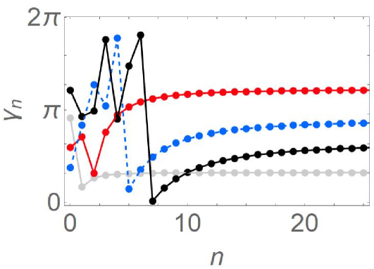
Figure 1: The geometric phase $\gamma_{n}$ [cf Eq. (44)] is given as a function of $n$ for the lowest basis states $\psi_{n}$ ($\gamma_{n}$ is plotted $\operatorname{mod}2\pi$). The system is a time-dependent oscillator with the frequency $\Omega(x,t)$ and the walls motion $L(t)$ given by Eqs. (46) and (45) resp. The black, blue dotted and red curves correspond to $\bar{L}_{0}=1000,800$, and 400 resp. while $\bar{L}_{0}=100$ is shown in light gray. Put differently, the curves correspond to $L_{0}=100$ and the scaling parameter $k=4$, $8$ and 10 ($q=0.1,\omega=1$, units with $\hbar,m,e=1$ are used).

IV.3 Confined time-dependent oscillators: Localized state

IV.3.1 Evolution of Gaussian state

The time-dependent boundary conditions induce geometric phases on the basis states $\psi_{n}$. Although a Gaussian state $G(x,0)$ initially given by Eq. (20) can be expanded at any time in terms of these basis states $\psi_{n}$ this does not imply of course that the evolved wavefunction $\psi(x,t)$ will also pick up a phase after a full cycle.

Actually, since Eqs. (16) and (19) still hold for the confined TDLO with moving walls, we can again write the time-evolved solution $\psi(x,T)$, here after a period $T$ in terms of a Theta function. Formally $\psi(x,t)$ is again given by Eq. (24), the only difference relative to the infinite potential well of Sec. III being that $L(t)$ is a periodic function and not linear in $t$. To assess the relevance of geometric phases, we rescale the walls motion while leaving the Hamiltonian invariant as explained above by putting $\bar{L}(t)=kL(t)$. We have seen that this rescaling modifies the geometric phases. Hence by comparing the rescaled wavefunction $\bar{\psi}(x,T)$ with the original solution $\psi(x,T),$ evolved in both cases from the same initial state $G(x,0),$ we can infer whether the geometric phases modify the quantum state evolution.

Writing $\bar{\psi}(x,T)/\psi(x,T)$ in terms of $\vartheta_{4}$ functions as per Eq. (24), and noting that $\bar{z}=z/k$, $\bar{\kappa}=\kappa/k^{2}$ and $L(T)=L_{0},$ we apply the Jacobi transformation (27) to find given by Eq. (20). From Eq. (25) we see that $\bar{z}=z/k$ and $\bar{\kappa}=\kappa/k^{2}$ so that by using Eq. (24) and the Jacobi transformation (27) we are led to

$$\frac{\bar{\psi}(x,T)}{\psi(x,T)}=\frac{\vartheta_{4}\left(\frac{1}{k}\frac{z}{\kappa},-k^{2}/\kappa\right)}{\vartheta_{4}\left(\frac{z}{\kappa},-1/\kappa\right)}.$$ (47)

The equality on the right handside holds only provided the conditions given above between Eqs. (29) and (33) hold (recall we have $k>1$). Under these circumstances we see, by following exactly the reasoning given above that both $\vartheta_{4}\left(\frac{1}{k}\frac{z}{\kappa},-k^{2}/\kappa\right)\simeq 1$ and $\vartheta_{4}\left(\frac{z}{\kappa},-1/\kappa\right)\simeq 1.$

Eq. (47) proves that while rescaling the walls motion changes the geometric phase of the basis functions according to $\bar{\gamma}_{n}=k^{2}\gamma_{n}$, no such change takes place when the initial state is the Gaussian $G(x,0)$ localized at the center of the confined time-dependent potential. The geometric phases picked up by each basis state over which $G(x,0)$ is expanded vanish by interference. Recall that an arbitrary initial Gaussian placed in a periodic (unconfined) potential is not cyclic unless specific conditions are verified child98 . Eq. (47) does not depend on whether these conditions are met and suggests that the wavefunction in the time-dependent boundary problem follows the same evolution as the one of the unconfined problem with the time-dependent potential: $\psi(x,T)$ can thus pick up a nonadiabatic cyclic geometric phase if the evolution in the unconfined potential leads to such a geometric phase, but there will be no additional effect due to the time-dependent boundaries.

IV.3.2 Approximate solution for an unconfined time-dependent oscillator

Note that as a byproduct of the present treatment, we have obtained an interesting closed form expression for the evolution of an initial Gaussian in an unconfined time-dependent linear oscillator potential for which there is a function $L(t)$ such that the frequency can be put under the form $\Omega^{2}(t)=-\partial_{t}^{2}L(t)/L(t)$. Indeed, Eq. (24) along with the Jacobi transformation (27) and $\vartheta_{4}\left(\frac{z}{\kappa},-1/\kappa\right)\simeq 1$ give the evolved Gaussian $\psi(x,t)$ as

$$\psi(x,t)=\frac{(1-i)\left(2\pi\right)^{1/4}e^{\frac{imx^{2}\partial_{t}L(t)}{2hL(t)}}}{\sqrt{-idL_{0}L(t)}\sqrt{\frac{1}{d^{2}}+\frac{2im}{hL_{0}}\partial_{t}L(t)_{t=0}}}\frac{e^{ix^{2}/\left[4\hbar L(t)^{2}\left(\frac{\tau(t)}{2m}+\frac{d^{2}}{-2d^{2}mL_{0}\partial_{t}L(t)_{t=0}+i\hbar L_{0}^{2}}\right)\right]}}{\sqrt{\frac{4\pi d^{2}\hbar}{L_{0}\left(\hbar L_{0}+2id^{2}m\partial_{t}L(t)_{t=0}\right)}+\frac{2i\pi\hbar\tau(t)}{m}}},$$ (48)

where $\tau(t)\equiv\int_{0}^{t}L^{-2}(t^{\prime})dt^{\prime}$. Contrary to the standard approaches for solving Gaussian problems in TDLOs, that involve nonlinear equations calling for numerical integration child98 ; matzkin2012 , Eq. (48) can be often obtained explicitly analytically, depending on whether the closed form integral of $\tau(t)$ is known (of course the range of application of Eq. (48) is very limited compared to standard methods).

IV.3.3 Example

Let us look at the localized state evolution for the TDLO whose geometric phases in the basis states were shown in Fig. 1. We start with an initial Gaussian state and let it evolve up to $t=T$ for the TDLO confined by infinitely high moving walls on the one hand, and for the same but unconfined TDLO on the other. Fig. 2 shows the real part of the evolved wavefunction in both cases. The curves are identical, illustrating that the walls motion has no influence on the evolution of a localized state. Note that the wavefunction for the unconfined TDLO has been computed by employing an independent and totally different method, based on Gaussian propagation through the solutions of Ermakov systems (see Ref. A2015JPA for details).

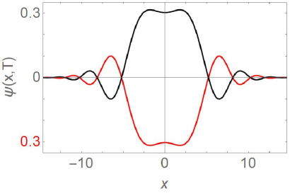
Figure 2: The state $\psi(x,t=T)$ evolved from an initial Gaussian [Eq. (20), here with $d=1$] in a confined oscillator with the time-dependent frequency given by Eq. (46) and the walls moving according to Eq. (45) with $L_{0}=100$ is compared to the state at $t=T$ evolved from the same initial Gaussian in the unconfined case (same Hamiltonian but without confining walls). The black line shows $\operatorname{Re}\psi(x,t)$ at $t=T$ (after one full cycle); the red line (upside-down) shows the evolution for the unconfined TDLO.

V Conclusion

To sum up we have shown that contrary to earlier claims, time-dependent boundary conditions do not induce an effective or explicit form of nonlocality, as happens eg for Bell correlations. This was seen to be the case for the paradigmatic particle in a box with moving walls and also holds for systems in which the moving boundaries induce geometric phases. Although a moving wall changes the boundary conditions, this change modifies the entire quantum state of the system (instantaneously in the non-relativistic framework) only if the state has a non-negligible amplitude in the boundary region. This is clearly not the case for a localized state placed far from the moving walls.

Appendix A Time evolved state in terms of theta functions

We first consider the case of an initial state given by the Gaussian

$$\left\langle x\right|\left.\mathcal{G}(t=0)\right\rangle\equiv\mathcal{G}(x,0)=\frac{e^{-\frac{(x-x_{0})^{2}}{4d^{2}}+\frac{ip_{0}x}{h}}}{\left(2\pi\right)^{1/4}\sqrt{d}}.$$ (49)

Contrary to the initial Gaussian given by Eq. (20), $\mathcal{G}(x,0)$ has its maximum at $x_{0}$ anywhere inside the box (but sufficiently far from the box boundaries, since by assumption the initial state has negligible amplitude at the boundaries), and a mean momentum $p_{0}$. In addition to the even basis functions (16) and (19) derived from the even instantaneous eigenstates $\phi_{n}(x,t)$ given by Eq. (6), we will also need odd basis functions derived in the same way from the odd eigenstates $\varphi_{n}(x,t)$ given by Eq. (7); for example the odd counterpart to $\psi_{n}(x,t)$ defined by Eq. (19) is

$$\zeta_{n}(x,t)=\sqrt{\frac{2}{L(t)}}e^{\frac{imx^{2}\left[\partial_{t}L(t)\right]}{2\hbar L(t)}-i\hbar\pi^{2}(2n)^{2}\int_{0}^{t}L(t^{\prime})^{-2}\,dt^{\prime}/2m}\sin\left(\pi(2n)x/L(t)\right).$$ (50)

The expansion coefficients $g_{n}$ of Eq. (21) now become

$$h_{n}(q) =\int_{-\infty}^{+\infty}\psi_{n}^{\ast}(x,0)\mathcal{G}(x,0)dx$$ (51)

$$=\frac{(1-i)\left(-\pi/2\right)^{1/4}e^{-\frac{x_{0}^{2}}{4d^{2}}}\left(e^{\frac{i\left[2\pi d^{2}\hbar(2n+1)+\left(2d^{2}p_{0}-i\hbar x_{0}\right)L_{0}\right]^{2}}{4d^{2}\hbar L_{0}\left(2d^{2}m\partial_{t}L(t)_{t=0}-i\hbar L_{0}\right)}}+e^{\frac{i\left[2\pi d^{2}\hbar(2n+1)+\left(-2d^{2}p_{0}+i\hbar x_{0}\right)L_{0}\right]^{2}}{4d^{2}\hbar L_{0}\left(2d^{2}m\partial_{t}L(t)_{t=0}-i\hbar L_{0}\right)}}\right)}{\sqrt{dL_{0}}\sqrt{\frac{1}{d^{2}}+\frac{2im\partial_{t}L(t)_{t=0}}{\hbar L_{0}}}}$$ (52)

for the even basis functions and

$$j_{n}(q) =\int_{-\infty}^{+\infty}\zeta_{n}^{\ast}(x,0)\mathcal{G}(x,0)dx$$ (53)

$$=\frac{i\left(2\pi\right)^{1/4}e^{-\frac{x_{0}^{2}}{4d^{2}}}e^{\frac{i\left[2\pi\hbar d^{2}(2n)+\left(-2d^{2}p_{0}+i\hbar x_{0}\right)L_{0}\right]^{2}}{4d^{2}\hbar L_{0}\left(2d^{2}m\partial_{t}L(t)_{t=0}-i\hbar L_{0}\right)}}-e^{{}^{\frac{i\left[2\pi\hbar d^{2}(2n)+\left(2d^{2}p_{0}-i\hbar x_{0}\right)L_{0}\right]^{2}}{4d^{2}\hbar L_{0}\left(2d^{2}m\partial_{t}L(t)_{t=0}-i\hbar L_{0}\right)}}}}{\sqrt{dL_{0}}\sqrt{\frac{1}{d^{2}}+\frac{2im\partial_{t}L(t)_{t=0}}{\hbar L_{0}}}}$$ (54)

for the odd basis functions.

It can be checked, after a tedious but straightforward calculation that the time evolved state $\psi(x,t)=\sum_{n\geqslant 0}h_{n}(q)\psi_{n}(x,t)+\sum_{n>0}j_{n}(q)\zeta_{n}(x,t)$ can be written in terms of 8 Jacobi theta functions, half of them being theta functions of the second type $\vartheta_{2}(z,\kappa)$ introduced above [Eq. (23)], the other half (for the odd part of the sum) being functions $\vartheta_{3}(z,\kappa)$ defined by

$$\vartheta_{3}(z,\kappa)=\sum_{n=-\infty}^{\infty}e^{i\pi\kappa n^{2}}e^{2inz}.$$ (55)

Put

$$A \equiv\exp\left(-\frac{x_{0}^{2}}{4d^{2}}+\frac{i\left(2d^{2}p_{0}-i\hbar x_{0}\right)^{2}L_{0}}{4d^{2}\hbar\left(2d^{2}m\partial_{t}L(t)_{t=0}-i\hbar L_{0}\right)}+\frac{imx^{2}\partial_{t}L(t)_{t=0}}{2\hbar L_{0}}\right)$$ (56)

$$B \equiv\sqrt{dL_{0}L(t)}\sqrt{\frac{1}{d^{2}}+\frac{2im\partial_{t}L(t)_{t=0}}{\hbar L_{0}}}$$ (57)

$$C \equiv\pi\frac{2d^{2}p_{0}-i\hbar x_{0}}{i\hbar L_{0}-2d^{2}m\partial_{t}L(t)_{t=0}}.$$ (58)

Note that $A$ and $C$ depend on $x_{0}$ and $p_{0}$. With $\kappa$ defined by Eq. (25) above, we introduce the functions

$$\theta_{1}(x,t;q) =(1-i)\left(-\pi\right)^{1/4}A\vartheta_{2}(-\frac{\pi x}{L(t)}-C,\kappa)/B$$ (59)

$$\theta_{2}(x,t;q) =(1-i)\left(-\pi\right)^{1/4}A\vartheta_{2}(\frac{\pi x}{L(t)}-C,\kappa)/B$$ (60)

$$\theta_{3}(x,t;q) =(1-i)\left(-\pi\right)^{1/4}A\vartheta_{2}(-\frac{\pi x}{L(t)}+C,\kappa)/B$$ (61)

$$\theta_{4}(x,t;q) =(1-i)\left(-\pi\right)^{1/4}A\vartheta_{2}(\frac{\pi x}{L(t)}+C,\kappa)/B$$ (62)

$$\theta_{5}(x,t;q) =\left(\frac{\pi}{2}\right)^{1/4}A\vartheta_{3}(-\frac{\pi x}{L(t)}-C,\kappa)/B$$ (63)

$$\theta_{6}(x,t;q) =-\left(\frac{\pi}{2}\right)^{1/4}A\vartheta_{3}(\frac{\pi x}{L(t)}-C,\kappa)/B$$ (64)

$$\theta_{7}(x,t;q) =-\left(\frac{\pi}{2}\right)^{1/4}A\vartheta_{3}(-\frac{\pi x}{L(t)}+C,\kappa)/B$$ (65)

$$\theta_{8}(x,t;q) =\left(\frac{\pi}{2}\right)^{1/4}A\vartheta_{3}(\frac{\pi x}{L(t)}+C,\kappa)/B.$$ (66)

Then the time-evolved state $\psi(x,t)$ analogous to the one obtained above [Eq. (24)] but when the initial state is the general Gaussian given by Eq. (49) is given in terms of the functions $\theta_{k}$ as

$$\psi(x,t;q)=\frac{1}{2}\sum_{k=1}^{8}\theta_{k}(x,t;q).$$ (67)

Appendix B Moving walls at constant velocity

Let us assess the effect of walls moving at constant velocity, discussed in Sec. III, on the wavefunction evolving from $\mathcal{G}(x,0)$. For each of the even functions $\theta_{k}$ ($k=1,..,4)$ the transformation (27) leads to the analog of Eq. (29) in the form

$$\frac{\theta_{k}(q=0)}{\theta_{k}(q)}=\frac{\vartheta_{4}\left(\frac{z_{k}(0)}{\kappa(0)},-1/\kappa(0)\right)}{\vartheta_{4}\left(\frac{z_{k}(q)}{\kappa(q)},-1/\kappa(q)\right)},\qquad k=1,..,4$$ (68)

where $z_{k}$ is the relevant argument of the theta function in the expression of $\theta_{k}$ given by Eqs. (59)-(62), that is $z_{k}=\pm\frac{\pi x}{L(t)}\pm C$.  As explained in Sec. III.2.3 in the case of a single theta function, this leads here, under the same assumptions, to $\theta_{k}(x,t;q=0)=\theta_{k}(x,t;q)$, so that the walls motion does not impinge on the evolution of each of these even functions $\theta_{k}$.

For the odd functions $\theta_{k}$ ($k=5,..,8)$ involving $\vartheta_{3},$ we use instead of Eq. (27) the Jacobi transformation bellman

$$\vartheta_{3}\left(z,\kappa\right)=\frac{e^{-iz^{2}/\kappa\pi}}{\left(-i\kappa\right)^{1/2}}\vartheta_{3}\left(\frac{z}{\kappa},-\frac{1}{\kappa}\right).$$ (69)

The result

$$\frac{\theta_{k}(q=0)}{\theta_{k}(q)}=\frac{\vartheta_{3}\left(\frac{z_{k}(0)}{\kappa(0)},-1/\kappa(0)\right)}{\vartheta_{3}\left(\frac{z_{k}(q)}{\kappa(q)},-1/\kappa(q)\right)}=1,\qquad k=5,..,8$$ (70)

is shown to hold by following the same arguments given in Sec. III.2.3, but by using the expansion (55) instead of (28). Thus Eq. (33) above stating that $\psi(x,t;q)=\psi(x,t;q=0)$ also holds when the initial state is the Gaussian (49) and $\psi(x,t;q)$ is given by Eq. (67).

Appendix C A single moving wall

In the main text we have considered the symmetric boundary conditions specified by Eq (4), as this gives a simpler treatment. However in most of the works greenberger ; makowski1992 ; zou2000 ; yao2001 ; wang2008 ; mousavi2012 ; mousavi2014 dealing with the subject of nonlocality induced by time-dependent boundary conditions, the problem of an infinite well with a single moving wall was considered. In that case, the Hamiltonian has the following boundary conditions:

$$H =\frac{P^{2}}{2m}+V$$ (71)

$$V(x,t) =\left\{\begin{array}[c]{l}0\text{ \ for}\ \ 0\leq x\leq L(t)\\ +\infty\text{ \ otherwise}\end{array}\right..$$ (74)

The instantaneous eigenstates of $H$ are similar to the odd functions $\varphi_{n}(x,t)$ introduced in Eq. (7) and the basis functions to the $\zeta_{n}(x,t)$ of Eq. (50); they are obtained by replacing in these expressions $n$ by $n/2,$ yielding

$$f_{n}(x,t)=\sqrt{2/L(t)}\sin\left[n\pi x/L(t)\right]$$ (75)

for the instantaneous eigenstates and

$$F_{n}(x,t)=\sqrt{\frac{2}{L(t)}}e^{\frac{imx^{2}\left[\partial_{t}L(t)\right]}{2\hbar L(t)}-i\hbar\pi^{2}n^{2}\int_{0}^{t}L(t^{\prime})^{-2}\,dt^{\prime}/2m}\sin\left(\pi nx/L(t)\right)$$ (76)

for the basis functions. Therefore, provided we are willing to keep the $-\infty$ bound in Eq. (53), a harmless approximation given the assumptions concerning the initial Gaussian, we can transpose the results obtained in the present Appendix [Eqs. (54), (63)-(66) and (70)] to the case of a single moving wall (note that relative to these expressions, the arguments of $\vartheta_{3}$ are rescaled as $z\rightarrow z/2$ and $\kappa\rightarrow\kappa/4$). Hence the conclusion concerning the non-relevance of the wall’s motion relative to the evolution of a state compactly localized inside the box also holds in this case.

References

- (1) N. C. Dias, A. Posilicano and J. N. Prata 2011, Commun. Pure Appl. Anal. 10 1687.
- (2) S. Di Martino, F. Anza, P. Facchi, A. Kossakowski, G. Marmo, A. Messina, B. Militello and S. Pascazio 2013, J. Phys. A 46 365301.
- (3) E. Knobloch and R. Krechetnikov 2015, Acta Appl. Math. 137 123.
- (4) S. W. Doescher and H. H. Rice 1969, Am. J. Phys. 37 1246
- (5) A.J. Makowski and S.T. Dembinski 1991, Phys. Lett. A 154 217
- (6) P. Pereshogin and P. Pronin 1991, Phys. Lett. A 156 2
- (7) A. Mostafazadeh 1999, J. Phys. A 32 8325
- (8) M.L. Glasser, J. Mateo, J. Negro, and L.M. Nieto 2009, Chaos Solitons Fract. 41 2067.
- (9) O. Fojon, M. Gadella and L. P. Lara 2010, Comput Math Appl 59, 264.
- (10) D. M. Greenberger Physica B 151 (1988) 374
- (11) A. J. Makowski and P. Peplowski 1992, Phys. Lett. A 163 142.
- (12) J. Zou and B. Shao 2000, Int. J. Mod. Phys. B 14 1059.
- (13) Q.K. Yao Qian-Kai, G. W. Ma, X. F. Chen and Y. Yu 2001, Int. J. Theor. Phys. 40 551.
- (14) Z. S. Wang, C. Wu, X. L Feng , L.C. Kwek, C.H. Lai, C.H. Oh and V. Vedral 2008, Phys. Lett. A 372 775
- (15) S. V. Mousavi 2012, EPL 99 30002.
- (16) S. V. Mousavi 2014, Phys. Scr. 89 065003.
- (17) P. Facchi, G. Garnero, G. Marmo and J. Samuel 2016, Ann. Phys. 372 201
- (18) R. Bellman, A brief introduction to Theta functions (Dover: Mineola, NY, 2013).
- (19) Y. Aharonov and J. Anandan 1987, Phys. Rev. Lett. 58 1593.
- (20) A. Bohm, A. Mostafazadeh, H. Koizumi, Q. Niu and J. Zwanziger, The Geometric Phase in Quantum Systems (Springer, Berlin, 2003).
- (21) J. S. Anandan 1988, Ann. Inst. Henri Poincaré 49 271.
- (22) A. Matzkin 2012, Phys. Rev. Lett. 109 150407
- (23) Y. C. Ge and M. S. Child 1997, Phys. Rev. Lett. 78 2507.
- (24) A. Matzkin 2015, J. Phys. A 48 305301