Kernel-based Discretisation for Solving Matrix-Valued PDEs

Abstract

In this paper, we discuss the solution of certain matrix-valued partial differential equations. Such PDEs arise, for example, when constructing a Riemannian contraction metric for a dynamical system given by an autonomous ODE. We develop and analyse a new meshfree discretisation scheme using kernel-based approximation spaces. However, since these approximation spaces have now to be matrix-valued, the kernels we need to use are fourth order tensors. We will review and extend recent results on even more general reproducing kernel Hilbert spaces. We will then apply this general theory to solve a matrix-valued PDE and derive error estimates for the approximate solution. The paper ends with a typical example from dynamical systems.

Keywords. Meshfree Methods, Radial Basis Functions, Autonomous Systems, Contraction Metric.

AMS subject classifications. 65N35, 65N15, 37B25, 37M99

1 Introduction

Kernel-based discretisation methods provide an extremely flexible, general framework to approximate the solution to even rather unconventional problems (see for example [7, 5, 42, 11, 13, 35]). They are meshfree methods, requiring only a discrete data set for discretising the underlying domain. Since the kernel can be chosen problem dependent, it is very easy to construct in particular smooth approximation spaces and high order methods.

Kernel-based methods have extensively been used for solving partial differential equation (see for example [15, 26, 12, 41]). They have been used in the context of dynamical systems for constructing Lyapunov functions ([17, 22]) and they also play a key role in learning theory ([8, 9, 31, 36, 39, 37]) and high-dimensional integration (see for example [10]) and many other areas.

It is the goal of this paper to derive and analyse a new method for reconstructing matrix-valued functions $M:\Omega\subseteq\mathbb{R}^{n}\to\mathbb{R}^{n\times n}$ from a matrix-valued PDE of the form

$$Df^{T}(x)M(x)+M(x)Df(x)+M^{\prime}(x)=-C(x),\qquad x\in\Omega\subseteq\mathbb{R}^{n}.$$ (1.1)

Here, $f$ and $C$ are given functions, defined on a given domain $\Omega\subseteq\mathbb{R}^{n}$. The function $f:\Omega\to\mathbb{R}^{n}$ is a differentiable vector-valued function with derivative matrix $Df:\Omega\to\mathbb{R}^{n\times n}$, $C:\Omega\to\mathbb{R}^{n\times n}$ is a matrix-valued function and $M^{\prime}$ is the so-called orbital derivative, i.e. it is component-wise defined to be $(M^{\prime}(x))_{ij}=\nabla M(x)_{ij}\cdot f(x)$.

Our work is motivated by a typical application of such matrix-valued PDEs from the theory of dynamical systems. To be more precise, when studying autonomous ODEs of the form $\dot{x}=f(x)$, then an exponentially stable equilibrium can be characterised by a Riemannian contraction metric [18]:

Theorem 1.

Let $\emptyset\not=G\subseteq\mathbb{R}^{n}$ be a compact, connected and positively invariant set and $M$ be a Riemannian contraction metric in $G$, i.e.

• $M\in C^{1}(G,\mathbb{R}^{n\times n})$, such that $M({x})$ is symmetric and positive definite for all ${x}\in G$.

• $D{f}({x})^{T}M({x})+M({x})D{f}({x})+M^{\prime}({x})$ is negative definite for all ${x}\in G$.

Then there exists one and only one equilibrium in ${x}_{0}$ in $G$; ${x}_{0}$ is exponentially stable and $G$ is a subset of the basin of attraction $A({x}_{0})$.

The difficulty of this approach is to constructively find such a contraction metric. In [18] a contraction metric is characterised as the solution of a first-order PDE of the form (1.1) for all ${x}\in\Omega=A(x_{0})$, where $C(x)=C\in\mathbb{R}^{n\times n}$ is a given symmetric and positive definite matrix. The construction of $M$ is thus a typical example of a matrix-valued PDE with the additional complication that the solution also has to be symmetric and positive definite.

In the accompanying paper [23], we will prove the theoretical results required in the dynamical system context. In this paper, however, we will concentrate on deriving the numerical framework for discretising even more general PDEs of the form

$$F(M)(x)=-C(x),\qquad x\in\Omega,$$ (1.2)

where $F$ is a rather general differential operator which maps matrix-valued Sobolev functions of order $\sigma$ to matrix-valued Sobolev functions of order $\tau<\sigma$.

The paper is organised as follows. In Section 2 we will review and extend results on general reproducing kernel Hilbert spaces, going far beyond the usual definition. In Section 3 we generalise the theory of optimal recovery to these general reproducing kernel Hilbert spaces. In Section 4 we will become more concrete by restricting ourselves to reproducing kernel Hilbert spaces of matrix-valued functions. In Section 5 we continue this by looking at Sobolev spaces of matrix-valued functions. In Section 6 we will derive error estimates for optimal recovery processes of solutions to (1.2). Section 7 then deals with the application to the above mentioned problem to construct a contraction metric for an autonomous system. The final section gives a numerical example.

2 Reproducing Kernel Hilbert Spaces

Reproducing Kernel Hilbert Spaces have first been introduced to describe real-valued functions $f\colon\Omega\to\mathbb{R}$ on a domain $\Omega\subseteq\mathbb{R}^{d}$ (see for example [2]). They require a kernel $\Phi:\Omega\times\Omega\to\mathbb{R}$ with the reproduction property $f(x)=\langle f,\Phi(\cdot,x)\rangle_{\mathcal{H}}$ for $f\in{\mathcal{H}}$, $x\in\Omega$ where ${\mathcal{H}}$ denotes a Hilbert space of functions $f:\Omega\to\mathbb{R}$. Later, so-called matrix-valued kernels $\Phi\colon\Omega\times\Omega\to\mathbb{R}^{n\times n}$ with the reproduction property $f(x)^{T}\alpha=\langle f,\Phi(\cdot,x)\alpha\rangle_{\mathcal{H}}$, have been introduced to recover vector-valued functions $f\colon\Omega\to\mathbb{R}^{n}$ where ${\mathcal{H}}$ denotes a Hilbert space of functions $\Omega\to\mathbb{R}^{n}$ and $\alpha\in\mathbb{R}^{n}$ is an arbitrary vector (see for example [1, 4, 16, 30, 32, 43]).

We are interested in reproducing kernel Hilbert spaces of matrix-valued functions. We start with a more general introduction, namely functions with values in a general Hilbert space $W$, which in the above examples was $\mathbb{R}$ and $\mathbb{R}^{n}$, respectively, and will later be the space $\mathbb{R}^{n\times n}$ of all real $n\times n$ matrices or the space $\mathbb{S}^{n\times n}$ of all symmetric real $n\times n$ matrices. The notion of such general reproducing kernel Hilbert spaces is not new, see for example [31] and the literature therein.

Let $W$ be a real Hilbert space and denote the linear space of all linear and bounded operators $L:W\to W$ by ${\mathcal{L}}(W)$. For any $L\in{\mathcal{L}}(W)$, we will denote the adjoint operator by $L^{*}\in{\mathcal{L}}(W)$.

Let $\Omega\subseteq\mathbb{R}^{d}$ be a given domain and let ${\mathcal{H}}(\Omega;W)$ be a Hilbert space of $W$-valued functions $f:\Omega\to W$.

Definition 2.

The Hilbert space ${\mathcal{H}}(\Omega;W)$ is called a reproducing kernel Hilbert space if there is a function $\Phi:\Omega\times\Omega\to{\mathcal{L}}(W)$ with

1. $\Phi(\cdot,x)\alpha\in{\mathcal{H}}(\Omega;W)$ for all $x\in\Omega$ and all $\alpha\in W$.

2. $\langle f(x),\alpha\rangle_{W}=\langle f,\Phi(\cdot,x)\alpha\rangle_{{\mathcal{H}}}$ for all $f\in{\mathcal{H}}(\Omega;W)$, all $x\in\Omega$ and all $\alpha\in W$.

The function $\Phi$ is called the reproducing kernel of ${\mathcal{H}}(\Omega;W)$.

Let us have a short look at two typical examples that have been introduced at the beginning of this section.

Example 3.

If we choose $W=\mathbb{R}$ with inner product being just the product, then ${\mathcal{H}}(\Omega;W)$ consists of real-valued functions. Moreover, each element $L$ of ${\mathcal{L}}(\mathbb{R})$ can be represented by $Lw=\ell w$ with $\ell\in\mathbb{R}$ and thus ${\mathcal{L}}(\mathbb{R})$ can be identified with $\mathbb{R}$. Hence, a reproducing kernel in this setting has to satisfy $\Phi(\cdot,x)\alpha\in{\mathcal{H}}(\Omega;W)$ for all $\alpha\in\mathbb{R}$, which is obviously equivalent to $\Phi(\cdot,x)\in{\mathcal{H}}(\Omega;W)$, and the second condition is equivalent to $f(x)=\langle f,\Phi(\cdot,x)\rangle_{\mathcal{H}}$. Hence, this is the classical reproducing kernel used in approximation theory and other areas.

Example 4.

If we choose $W=\mathbb{R}^{n}$ with the standard inner product, then $\Phi$ has to map into the linear mappings from $\mathbb{R}^{n}\to\mathbb{R}^{n}$ and can hence be represented by a matrix. Thus, $\Phi(\cdot,x)\alpha$ represents now a vector-valued function and the second condition in the definition becomes

$$f(x)^{T}\alpha=\langle f,\Phi(\cdot,x)\alpha\rangle_{\mathcal{H}}.$$

This is usually referred to as matrix-valued kernels in the literature.

Before we come to our specific situation, we want to point out a few general results, see also [31].

Lemma 5.

1. The reproducing kernel $\Phi$ of a Hilbert space ${\mathcal{H}}(\Omega;W)$ is uniquely determined.

2. The reproducing kernel satisfies $\Phi(x,y)^{*}=\Phi(y,x)$ for all $x,y\in\Omega$.

3. The reproducing kernel is positive semi-definite, i.e. it satisfies

   $$\sum_{i,j=1}^{N}\left\langle\alpha_{i},\Phi(x_{i},x_{j})\alpha_{j}\right\rangle_{W}\geq 0$$

   for all $x_{1},\ldots,x_{N}\in\Omega$ and all $\alpha_{1},\ldots,\alpha_{N}\in W$.

Proof.

The first property is proven as in the classical reproducing kernel setting by assuming that there are two kernels and showing that they have to be the same using the reproduction property. The second property follows by setting $f=\Phi(\cdot,y)\beta$ in the reproduction formula. This yields

$$\langle\Phi(x,y)\beta,\alpha\rangle_{W} = \langle\Phi(\cdot,y)\beta,\Phi(\cdot,x)\alpha\rangle_{\mathcal{H}}=\langle\Phi(\cdot,x)\alpha,\Phi(\cdot,y)\beta\rangle_{\mathcal{H}}$$

$$= \langle\Phi(y,x)\alpha,\beta\rangle_{W}=\langle\beta,\Phi(y,x)\alpha\rangle_{W}.$$

The third property simply follows from

$$\sum_{i,j=1}^{N}\left\langle\alpha_{i},\Phi(x_{i},x_{j})\alpha_{j}\right\rangle_{W} = \sum_{i,j=1}^{N}\left\langle\Phi(x_{j},x_{i})\alpha_{i},\alpha_{j}\right\rangle_{W}=\sum_{i,j=1}^{N}\langle\Phi(\cdot,x_{i})\alpha_{i},\Phi(\cdot,x_{j})\alpha_{j}\rangle_{\mathcal{H}}$$

$$= \left\|\sum_{i=1}^{N}\Phi(\cdot,x_{i})\alpha_{i}\right\|_{{\mathcal{H}}}^{2}\geq 0.$$

∎

In most cases, the kernel is even positive definite, namely if the functions $\Phi(\cdot,x_{j})\alpha_{j}$ are linearly independent.

Definition 6.

A kernel $\Phi:\Omega\times\Omega\to{\mathcal{L}}(W)$ which satisfies $\Phi(x,y)^{*}=\Phi(y,x)$ for all $x,y\in\Omega$ is called positive definite if for all $N\in\mathbb{N}$, for all $x_{1},\ldots,x_{N}\in\Omega$, pairwise distinct, and for all $\alpha_{1},\ldots,\alpha_{N}\in W$, not all of them zero, we have

$$\sum_{i,j=1}^{N}\left\langle\alpha_{i},\Phi(x_{i},x_{j})\alpha_{j}\right\rangle_{W}>0.$$

As usual in the theory of reproducing kernel Hilbert spaces, it is also possible to start with a kernel and to build its Hilbert space from scratch. This is done as follows. Suppose we have a positive definite kernel $\Phi:\Omega\times\Omega\to{\mathcal{L}}(W)$ as in Definition 6. Then, we can form the space

$${\mathcal{F}}_{\Phi}(\Omega;W)=\mbox{span}\left\{\Phi(\cdot,x)\alpha:x\in\Omega,\alpha\in W\right\}$$

and equip this space with an inner product defined by

$$\langle\Phi(\cdot,x)\alpha,\Phi(\cdot,y)\beta\rangle_{\Phi}:=\langle\Phi(x,y)\beta,\alpha\rangle_{W}.$$

The closure of ${\mathcal{F}}_{\Phi}(\Omega;W)$ with respect to the norm induced by this inner product is then the corresponding Hilbert space ${\mathcal{H}}(\Omega;W)$ for which $\Phi$ is the reproducing kernel.

3 Optimal Recovery

If $\Phi:\Omega\times\Omega\to{\mathcal{L}}(W)$ is a positive definite kernel, then this immediately implies that we can solve the following interpolation problem uniquely.

Theorem 7.

If $x_{1},\ldots,x_{N}$ are pairwise distinct points from $\Omega$ and if $f_{1},\ldots,f_{N}\in W$ are given, then there is exactly one interpolant of the form

$$s_{f}(x)=\sum_{j=1}^{N}\Phi(x,x_{j})\alpha_{j}$$

which satisfies $s_{f}(x_{i})=f_{i}$, $1\leq i\leq N$.

Proof.

Let $W^{N}$ denote the Cartesian product of the Hilbert space $W$. Then, $W^{N}$ becomes a Hilbert space itself if equipped with the inner product

$$\langle\alpha,\beta\rangle_{W^{N}}=\sum_{j=1}^{N}\langle\alpha_{j},\beta_{j}\rangle_{W}.$$

The matrix $A:=(\Phi(x_{i},x_{j}))_{1\leq i,j\leq N}$ defines a linear mapping $A:W^{N}\to W^{N}$, which is self-adjoint because of the second statement in Lemma 5:

$$\langle A\alpha,\beta\rangle_{W^{N}} = \sum_{i=1}^{N}\langle(A\alpha)_{i},\beta_{i}\rangle_{W}=\sum_{i=1}^{N}\sum_{j=1}^{N}\langle\Phi(x_{i},x_{j})\alpha_{j},\beta_{i}\rangle_{W}$$

$$= \sum_{i=1}^{N}\sum_{j=1}^{N}\langle\alpha_{j},\Phi(x_{j},x_{i})\beta_{i}\rangle_{W}=\sum_{j=1}^{N}\langle\alpha_{j},(A\beta)_{j}\rangle_{W}$$

$$= \langle\alpha,A\beta\rangle_{W^{N}}.$$

Thus, the relation $\ker(A^{*})=\operatorname{range}(A)^{\bot}$ shows together with $A=A^{*}$ that $A$ is injective if and only if $A$ is surjective. But injectivity follows directly from the fact that $\Phi$ is positive definite. ∎

Within this general framework, we now want to discuss the more general concept of optimal recovery. Hence, let ${\mathcal{H}}(\Omega;W)$ be our reproducing kernel Hilbert space with reproducing kernel $\Phi:\Omega\times\Omega\to{\mathcal{L}}(W)$. As usual, we denote the dual of ${\mathcal{H}}(\Omega;W)$ by ${\mathcal{H}}(\Omega;W)^{*}$.

Definition 8.

Given $N$ linearly independent functionals $\lambda_{1},\ldots,\lambda_{N}\in{\mathcal{H}}(\Omega;W)^{*}$ and $N$ values $f_{1}=\lambda_{1}(f),\ldots,f_{N}=\lambda_{N}(f)\in\mathbb{R}$ generated by an element $f\in{\mathcal{H}}(\Omega;W)$. The optimal recovery of $f$ based on this information is defined to be the element $s^{*}\in{\mathcal{H}}(\Omega;W)$ which solves

$$\min\left\{\|s\|_{\mathcal{H}}:s\in{\mathcal{H}}(\Omega;W)\mbox{ with }\lambda_{j}(s)=f_{j},1\leq j\leq N\right\}.$$

The solution to this minimisation problem is well-known and follows directly from standard Hilbert space theory; it works in any Hilbert space, not only in reproducing kernel Hilbert spaces. We quote the following result from [42, Theorem 16.1]:

Theorem 9.

Let $H$ be a Hilbert space. Let $\lambda_{1},\ldots,\lambda_{N}\in H^{*}$ be linearly independent linear functionals with Riesz representers $v_{1},\ldots,v_{N}\in H$. Then the element $s^{*}\in H$ which solves

$$\min\{\|s\|_{H}:s\in H\mbox{ with }\lambda_{j}(s)=f_{j},1\leq j\leq N\}$$

is given by

$$s^{*}=\sum_{k=1}^{N}\beta_{k}v_{k},$$

where the coefficients $\beta_{k}\in\mathbb{R}$ are determined by the generalised interpolation conditions $\lambda_{i}(s^{*})=f_{i}$, $1\leq i\leq N$, which lead to the linear system $A_{\Lambda}\beta=f$ with the positive definite matrix $A_{\Lambda}=(a_{ik})$ having entries $a_{ik}=\lambda_{i}(v_{k})=\langle v_{k},v_{i}\rangle_{H}$.

Returning to our specific situation $H={\mathcal{H}}(\Omega;W)$, to apply this theorem, we will need to know the Riesz representers of our functionals $\lambda\in{\mathcal{H}}(\Omega;W)^{*}$. We start with rather specific functionals.

Lemma 10.

Let $\lambda\in{\mathcal{H}}(\Omega;W)^{*}$ be of the form $\lambda(f)=\langle f(x),\alpha\rangle_{W}$, $f\in{\mathcal{H}}(\Omega;W)$ with fixed $x\in\Omega$ and $\alpha\in W$. Then, $\lambda=\lambda_{x,\alpha}$ has the Riesz representer

$$v_{\lambda}=\Phi(\cdot,x)\alpha\in{\mathcal{H}}(\Omega;W).$$

Proof.

This simply follows from applying $\lambda_{x,\alpha}$ to the specific function $f=\Phi(\cdot,y)\beta$ with $y\in\Omega$ and $\beta\in W$. Using the definition of the functional and the reproducing kernel property yields

$$\lambda_{x,\alpha}(\Phi(\cdot,y)\beta)=\langle\Phi(x,y)\beta,\alpha\rangle_{W}=\langle\Phi(\cdot,y)\beta,\Phi(\cdot,x)\alpha\rangle_{{\mathcal{H}}}.$$

However, we also have by the Riesz representation theorem that

$$\lambda_{x,\alpha}(\Phi(\cdot,y)\beta)=\langle\Phi(\cdot,y)\beta,v_{\lambda}\rangle_{{\mathcal{H}}}.$$

Since the functions $\Phi(\cdot,y)\beta$ are dense in ${\mathcal{H}}(\Omega;W)$, this gives $v_{\lambda}=\Phi(\cdot,x)\alpha$. ∎

The result for arbitrary functionals can be reduced to this special case.

Proposition 11.

Assume that $\{\alpha_{j}\}_{j\in J}$ is an orthonormal basis of $W$. Then, the Riesz representer of a functional $\lambda\in{\mathcal{H}}(\Omega;W)^{*}$ is given by

$$v_{\lambda}(x)=\sum_{j\in J}\lambda(\Phi(\cdot,x)\alpha_{j})\alpha_{j},\qquad x\in\Omega.$$

Proof.

Since $v_{\lambda}(x)\in W$ for every $x\in\Omega$ and since $\{\alpha_{j}\}_{j\in J}$ is an orthonormal basis of $W$, we can expand $v_{\lambda}(x)$ within this basis using its Fourier representation

$$v_{\lambda}(x)=\sum_{j\in J}\langle v_{\lambda}(x),\alpha_{j}\rangle_{W}\alpha_{j}.$$

The result then follows immediately from the reproducing kernel property:

$$\langle v_{\lambda}(x),\alpha_{j}\rangle_{W}=\langle v_{\lambda},\Phi(\cdot,x)\alpha_{j}\rangle_{{\mathcal{H}}}=\langle\Phi(\cdot,x)\alpha_{j},v_{\lambda}\rangle_{{\mathcal{H}}}=\lambda(\Phi(\cdot,x)\alpha_{j}).$$

∎

Thus, the optimal recovery problem can be recast as a linear system. From now on, we will write $\lambda^{y}(\Phi(y,x)\alpha)$ to indicate that the functional $\lambda$ acts on the variable $y$ of the kernel.

Corollary 12.

Assume that $\{\alpha_{j}\}_{j\in J}$ is an orthonormal basis of $W$. The solution of the minimisation problem of Theorem 9 is given by

$$s^{*}=\sum_{k=1}^{N}\beta_{k}\sum_{j\in J}\lambda_{k}^{y}(\Phi(y,\cdot)\alpha_{j})\alpha_{j},$$

and the coefficients $\beta_{k}\in\mathbb{R}$ are determined by

$$\sum_{k=1}^{N}\lambda_{i}^{x}\left[\lambda_{k}^{y}\sum_{j\in J}\left(\Phi(y,x)\alpha_{j}\right)\alpha_{j}\right]\beta_{k}=f_{i},\qquad 1\leq i\leq N.$$

Example 13.

Let us again have look at vector-valued functions, i.e. we let $W=\mathbb{R}^{n}$. Then, we can choose the standard basis $(e_{j})_{j=1,\ldots,n}$ of $\mathbb{R}^{n}$ as the orthonormal basis and hence, the optimal recovery is given by

$$s^{*}=\sum_{k=1}^{N}\beta_{k}\sum_{j=1}^{n}\lambda_{k}^{y}(\Phi(y,\cdot)e_{j})e_{j}.$$

Here, $\Phi(x,y)\in\mathbb{R}^{n\times n}$ is a matrix and thus $\Phi(x,y)e_{j}$ gives the $j$th column of this matrix. This shows that the expression $\lambda_{k}^{y}(\Phi(y,\cdot)e_{j})$ means applying $\lambda_{k}$ to the $j$th column (or row since $\Phi$ is symmetric) of $\Phi(y,\cdot)$ with respect to $y$. Hence, we can define $\lambda_{k}^{y}\Phi(y,\cdot)$ simply by applying $\lambda_{k}^{y}$ to each column/row of $\Phi(y,\cdot)$, which altogether results into a vector. Moreover, with this definition, we can simply write

$$\sum_{j=1}^{n}\lambda_{k}^{y}(\Phi(y,\cdot)e_{j})e_{j}=\lambda_{k}^{y}\Phi(y,\cdot)$$

and hence

$$s^{*}=\sum_{k=1}^{N}\beta_{k}\lambda_{k}^{y}\Phi(y,\cdot),$$

which is a vector-valued function. Finally, the coefficients $\beta_{k}$ are simply determined by solving $A\beta=f$ with $A$ having entries $\lambda_{i}^{x}\lambda_{k}^{y}\Phi(y,x)$.

After establishing the general theory, we will in the following sections consider special cases. In particular, we will choose $W$ to be the space $\mathbb{R}^{n\times n}$ of real-valued $n\times n$ matrices or its subspace $\mathbb{S}^{n\times n}$ of symmetric matrices (Section 4). Then we will consider specific RKHS spaces, namely matrix-valued Sobolev spaces $H^{\sigma}(\Omega;\mathbb{S}^{n\times n})$ in Section 5, where the kernel is built from the kernel of the corresponding real-valued Sobolev space. Finally, we will consider functionals of the form $\lambda_{k}^{(i,j)}(M):=e_{i}^{T}F(M)(x_{k})e_{j}$, where $F\colon H^{\sigma}(\Omega;\mathbb{S}^{n\times n})\to H^{\tau}(\Omega;\mathbb{S}^{n\times n})$ is a linear and bounded operator, in particular differential operator, and derive error estimates in Section 6. In Section 7, a specific linear operator $F$ from dynamical systems will be considered.

4 Matrix-Valued Theory

We are now interested in matrix-valued functions, i.e. we set $W=\mathbb{R}^{n\times n}$ or $W=\mathbb{S}^{n\times n}$, the space of all symmetric $n\times n$ matrices. On $W$ we define the following inner product to make it a Hilbert space.

$$\langle\alpha,\beta\rangle_{W} = \sum_{i,j=1}^{n}\alpha_{ij}\beta_{ij},\qquad\alpha=(\alpha_{ij}),\beta=(\beta_{ij}).$$ (4.1)

A kernel $\Phi$ is now a mapping $\Phi:\Omega\times\Omega\to{\mathcal{L}}(\mathbb{R}^{n\times n})$ and can be represented by a tensor of order $4$, i.e. we will write $\Phi=(\Phi_{ijk\ell})$ and define its action on $\alpha\in\mathbb{R}^{n\times n}$ by

$$(\Phi(x,y)\alpha)_{ij} = \sum_{k,\ell=1}^{n}\Phi(x,y)_{ijk\ell}\alpha_{k\ell}.$$ (4.2)

By 2. of Lemma 5, a necessary requirement for the kernel is the adjoint condition $\langle\Phi(x,y)\alpha,\beta\rangle_{W}=\langle\alpha,\Phi(y,x)\beta\rangle_{W}$, which means

$$\sum_{i,j=1}^{n}\sum_{k,\ell=1}^{n}\Phi(x,y)_{ijk\ell}\alpha_{k\ell}\beta_{ij} = \sum_{i,j=1}^{n}\sum_{k,\ell=1}^{n}\Phi(y,x)_{ijk\ell}\alpha_{ij}\beta_{k\ell}$$

$$= \sum_{i,j=1}^{n}\sum_{k,\ell=1}^{n}\Phi(y,x)_{k\ell ij}\alpha_{k\ell}\beta_{ij}.$$

Hence, we require

$$\Phi(x,y)_{ijk\ell}=\Phi(y,x)_{k\ell ij}.$$ (4.3)

This will motivate the choice of a kernel in (5.1) in the next section. The kernel $\Phi$ is positive definite, see Definition 6, if

$$\sum_{\mu,\nu=1}^{N}\langle\alpha^{(\nu)},\Phi(x_{\nu},x_{\mu})\alpha^{(\mu)}\rangle_{W}=\sum_{\mu,\nu=1}^{N}\sum_{i,j=1}^{n}\sum_{k,\ell=1}^{n}\Phi(x_{\nu},x_{\mu})_{ijk\ell}\alpha^{(\nu)}_{ij}\alpha^{(\mu)}_{k\ell}\geq 0$$ (4.4)

and the sum is positive if not all of the $\alpha^{(\nu)}$ are zero. The associated reproducing kernel Hilbert space ${\mathcal{H}}(\Omega;W)={\mathcal{H}}(\Omega;\mathbb{R}^{n\times n})$ consists of matrix-valued functions.

Finally, for a given functional $\lambda\in{\mathcal{H}}(\Omega;\mathbb{R}^{n\times n})^{*}$, we can write its Riesz representer as follows. Let $E_{\mu\nu}\in\mathbb{R}^{n\times n}$ be the matrix with value $1$ at position $(\mu,\nu)$ and value zero everywhere else. Then, $\{E_{\mu\nu}:1\leq\mu,\nu\leq n\}$ is an orthonormal basis of $W=\mathbb{R}^{n\times n}$ and the Riesz representer of $\lambda$ hence becomes by Proposition 11

$$v_{\lambda}(x)=\sum_{\mu,\nu=1}^{n}\lambda(\Phi(\cdot,x)E_{\mu\nu})E_{\mu\nu},\qquad x\in\Omega.$$

In the case of the symmetric matrices, we have a similar result, however, we need to consider a different orthonormal basis, namely $\{E^{s}_{\mu\nu}:1\leq\mu\leq\nu\leq n\}$. We define $E^{s}_{\mu\mu}$ to be the matrix with value 1 at position $(\mu,\mu)$ and value zero everywhere else. For $\mu<\nu$, we define $E^{s}_{\mu\nu}$ to be the matrix with value $1/\sqrt{2}$ at positions $(\mu,\nu)$ and $(\nu,\mu)$ and value zero everywhere else. It is easy to see that $\{E^{s}_{\mu\nu}:1\leq\mu\leq\nu\leq n\}$ is an orthonormal basis of $W=\mathbb{S}^{n\times n}$.

For a given functional $\lambda\in{\mathcal{H}}(\Omega;\mathbb{S}^{n\times n})^{*}$, the Riesz representer of $\lambda$ hence is by Proposition 11

$$v_{\lambda}(x) = \sum_{1\leq\mu\leq\nu\leq n}\lambda(\Phi(\cdot,x)E^{s}_{\mu\nu})E^{s}_{\mu\nu},\qquad x\in\Omega.$$ (4.5)

5 Matrix-Valued Sobolev Spaces

In the following, we will be concerned with specific functionals defined on specific reproducing kernel Hilbert spaces. We start with discussing the spaces.

Throughout this paper, we will assume that $H^{\sigma}(\Omega)$ denotes the Sobolev space of order $\sigma>d/2$, where the weak derivatives are measured in the $L_{2}(\Omega)$-norm. However, $\sigma$ does not necessarily have to be an integer and the space can then be defined, for example, by interpolation. We will always assume that $\sigma>d/2$ such that the Sobolev embedding theorem yields $H^{\sigma}(\Omega)\subseteq C(\Omega)$ which particularly means that $H^{\sigma}(\Omega)$ has a reproducing kernel. The kernel is uniquely determined by the inner product, but different equivalent inner products allow us to choose different kernels. Examples of such kernels comprise of the Sobolev (or Matern) kernels and Wendland’s radial basis functions (see [11, 40, 34]).

We will also assume that $\Omega\subseteq\mathbb{R}^{d}$ is a bounded domain with a boundary which is at least Lipschitz continuous.

Definition 14.

Let $\Omega\subseteq\mathbb{R}^{d}$ and $\sigma>d/2$ be given. Then, the matrix-valued Sobolev space $H^{\sigma}(\Omega;\mathbb{R}^{n\times n})$ consists of all matrix-valued functions $M$ having each component $M_{ij}$ in $H^{\sigma}(\Omega)$. Similarly, the Sobolev space $H^{\sigma}(\Omega;\mathbb{S}^{n\times n})$ consists of all symmetric matrix-valued functions $M$ having each component $M_{ij}$ in $H^{\sigma}(\Omega)$.

$H^{\sigma}(\Omega;\mathbb{R}^{n\times n})$ and $H^{\sigma}(\Omega;\mathbb{S}^{n\times n})$ are Hilbert spaces with inner product given by

$$\langle M,S\rangle_{H^{\sigma}(\Omega;\mathbb{R}^{n\times n})}:=\sum_{i,j=1}^{n}\langle M_{ij},S_{ij}\rangle_{H^{\sigma}(\Omega)};$$

the same inner product can be used for $H^{\sigma}(\Omega;\mathbb{S}^{n\times n})$. They are also reproducing kernel Hilbert spaces.

Lemma 15.

Let $\Omega\subseteq\mathbb{R}^{d}$ and $\sigma>d/2$ be given. Assume that $\phi:\Omega\times\Omega\to\mathbb{R}$ is a reproducing kernel of $H^{\sigma}(\Omega)$. Then, $H^{\sigma}(\Omega;\mathbb{R}^{n\times n})$ and $H^{\sigma}(\Omega;\mathbb{S}^{n\times n})$ are also reproducing kernel Hilbert spaces with reproducing kernel $\Phi$ defined by

$$\Phi(x,y)_{ijk\ell}:=\phi(x,y)\delta_{ik}\delta_{j\ell}$$ (5.1)

for $x,y\in\Omega$ and $1\leq i,j,k,\ell\leq n$.

Proof.

We have to verify the two defining properties of a reproducing kernel, see Definition 2. First of all, we obviously have $\Phi(\cdot,x)\alpha\in H^{\sigma}(\Omega;\mathbb{R}^{n\times n})$ for all $x\in\Omega$ and all $\alpha\in\mathbb{R}^{n\times n}$ since

$$(\Phi(\cdot,x)\alpha)_{ij}=\sum_{k,\ell=1}^{n}\Phi(\cdot,x)_{ijk\ell}\alpha_{k\ell}=\sum_{k,\ell=1}^{n}\phi(\cdot,x)\delta_{ik}\delta_{j\ell}\alpha_{k\ell}=\phi(\cdot,x)\alpha_{ij}$$

and $\phi$ is a reproducing kernel of $H^{\sigma}(\Omega)$. For $H^{\sigma}(\Omega;\mathbb{S}^{n\times n})$, note that $\Phi(\cdot,x)\alpha$ is symmetric if $\alpha$ is symmetric.

Secondly, we have the reproduction property. If once again $\alpha\in\mathbb{R}^{n\times n}$ and $f\in H^{\sigma}(\Omega;\mathbb{R}^{n\times n})$ then the computation just made shows

$$\langle f,\Phi(\cdot,x)\alpha\rangle_{H^{\sigma}(\Omega;\mathbb{R}^{n\times n})} = \sum_{i,j=1}^{n}\langle f_{ij},(\Phi(\cdot,x)\alpha)_{ij}\rangle_{H^{\sigma}(\Omega)}$$

$$= \sum_{i,j=1}^{n}\langle f_{ij},\phi(\cdot,x)\alpha_{ij}\rangle_{H^{\sigma}(\Omega)}$$

$$= \sum_{i,j=1}^{n}\alpha_{ij}f_{ij}(x)=\langle f(x),\alpha\rangle_{\mathbb{R}^{n\times n}},$$

using the reproduction property of $\phi$ in $H^{\sigma}(\Omega)$. The proof for $H^{\sigma}(\Omega;\mathbb{S}^{n\times n})$ is the same. ∎

Corollary 16.

Let the assumptions of Lemma 15 hold with a positive definite kernel $\phi:\Omega\times\Omega\to\mathbb{R}$. Then, also the matrix-valued kernel $\Phi$ is positive definite.

Proof.

The kernel is positive definite in the sense of (4.4), since we have

$$\sum_{\mu,\nu=1}^{N}\sum_{i,j=1}^{n}\sum_{k,\ell=1}^{n}\Phi(x_{\nu},x_{\mu})_{ijk\ell}\alpha^{(\nu)}_{ij}\alpha^{(\mu)}_{k\ell} = \sum_{\mu,\nu=1}^{N}\sum_{i,j=1}^{n}\sum_{k,\ell=1}^{n}\phi(x_{\nu},x_{\mu})\delta_{ik}\delta_{j\ell}\alpha^{(\nu)}_{ij}\alpha^{(\mu)}_{k\ell}$$

$$= \sum_{i,j=1}^{n}\sum_{\mu,\nu=1}^{N}\phi(x_{\nu},x_{\mu})\alpha_{ij}^{(\nu)}\alpha_{ij}^{(\mu)}\geq 0$$

and at least one of the inner sums is positive. ∎

Next, we will discuss the functionals on $H^{\sigma}(\Omega;\mathbb{R}^{n\times n})$ and $H^{\sigma}(\Omega;\mathbb{S}^{n\times n})$ that we are interested in. Note that using a kernel of the form (5.1) together with point evaluations would simply lead to a component-wise treatment. Hence, in this situation, dealing with each component separately would be more efficient.

Here, however, we are interested in the following situation. Suppose $F:H^{\sigma}(\Omega;\mathbb{R}^{n\times n})\to H^{\tau}(\Omega;\mathbb{R}^{n\times n})$ (or $F:H^{\sigma}(\Omega;\mathbb{S}^{n\times n})\to H^{\tau}(\Omega;\mathbb{S}^{n\times n})$) is a linear and bounded map, i.e. there is a constant $C>0$ such that

$$\|F(M)\|_{H^{\tau}(\Omega;\mathbb{R}^{n\times n})}\leq C\|M\|_{H^{\sigma}(\Omega;\mathbb{R}^{n\times n})},\qquad M\in H^{\sigma}(\Omega;\mathbb{R}^{n\times n}).$$

Suppose further that $\tau>d/2$ so that $F(M)\in C(\Omega;\mathbb{R}^{n\times n})$ is continuous. Then, we can define functionals of the form

$$\lambda_{k}^{(i,j)}(M)=e_{i}^{T}F(M)(x_{k})e_{j}$$

for $1\leq i,j\leq n$ (or $1\leq i\leq j\leq n$) and $1\leq k\leq N$, where $X=\{x_{1},\ldots,x_{N}\}$ is a given discrete point set in $\Omega$.

We will specify the mapping $F$ later on but we can derive a general theory using just these assumptions.

6 Error Analysis

In this section we will start with analysing the reconstruction error. Here, we will follow general ideas from scattered data approximation. In particular, we will measure the error in terms of the so-called fill distance or mesh norm

$$h_{X,\Omega}:=\sup_{x\in\Omega}\min_{x_{i}\in X}\|x-x_{i}\|_{2}.$$

This means that we can derive the classical error estimates based upon sampling inequalities also in this case. We will require the following result (see [33]).

Lemma 17.

Let $\Omega\subseteq\mathbb{R}^{d}$ be a bounded domain with Lipschitz continuous boundary. Let $\sigma>d/2$ and let $X=\{x_{1},\ldots,x_{N}\}\subseteq\Omega$. If $f\in H^{\sigma}(\Omega)$ vanishes on $X$, then there is a constant $C>0$ independent of $X$ and $f$ such that

$$\|f\|_{L_{\infty}(\Omega)}\leq Ch_{X,\Omega}^{\sigma-d/2}\|f\|_{H^{\sigma}(\Omega)}.$$

We can now use this result component-wise to derive estimates for the matrix-valued set-up. We will do this immediately for the situation we are interested in, which gives our first main result of this paper.

Theorem 18.

Let $\Omega\subseteq\mathbb{R}^{d}$ be a bounded domain with Lipschitz continuous boundary. Let $\sigma,\tau>d/2$ be given and let $F:H^{\sigma}(\Omega;\mathbb{R}^{n\times n})\to H^{\tau}(\Omega;\mathbb{R}^{n\times n})$ ($F:H^{\sigma}(\Omega;\mathbb{S}^{n\times n})\to H^{\tau}(\Omega;\mathbb{S}^{n\times n})$) be linear and bounded. Finally, let $X=\{x_{1},\ldots,x_{N}\}\subseteq\Omega$ be given and let

$$\lambda_{k}^{(i,j)}(M):=e_{i}^{T}F(M)(x_{k})e_{j},\qquad 1\leq k\leq N,\quad 1\leq i,j\leq n\quad(1\leq i\leq j\leq n).$$

Then each $\lambda_{k}^{(i,j)}$ belongs to the dual of $H^{\sigma}(\Omega;\mathbb{R}^{n\times n})$ ($H^{\sigma}(\Omega;\mathbb{S}^{n\times n})$).

Let us further assume that they are linearly independent. If $S$ denotes the optimal recovery of $M\in H^{\sigma}(\Omega;\mathbb{R}^{n\times n})$ ($H^{\sigma}(\Omega;\mathbb{S}^{n\times n})$) in the sense of Definition 8 using these functionals and a reproducing kernel of $H^{\sigma}(\Omega;\mathbb{R}^{n\times n})$ ($H^{\sigma}(\Omega;\mathbb{S}^{n\times n})$), then

$$\|F(M)-F(S)\|_{L_{\infty}(\Omega;\mathbb{R}^{n\times n})}\leq Ch_{X,\Omega}^{\tau-d/2}\|M\|_{H^{\sigma}(\Omega;\mathbb{R}^{n\times n})},$$

where $\|A\|_{L_{\infty}(\Omega;\mathbb{R}^{n\times n})}=\max_{i,j=1,\ldots,n}\|a_{ij}(x)\|_{L_{\infty}(\Omega)}$.

Proof.

We only consider the case $\mathbb{R}^{n\times n}$ as the proof for $\mathbb{S}^{n\times n}$ is similar. Obviously, the $\lambda_{k}^{(i,j)}$ are linear. Because of our assumptions, $F(M)$ is indeed continuous by the Sobolev embedding theorem, i.e. the functionals are well-defined. Furthermore,

$$|\lambda_{k}^{(i,j)}(M)|\leq C\|F(M)\|_{H^{\tau}(\Omega;\mathbb{R}^{n\times n})}\leq C\|M\|_{H^{\sigma}(\Omega;\mathbb{R}^{n\times n})},\qquad M\in H^{\sigma}(\Omega;\mathbb{R}^{n\times n}),$$

by the Sobolev embedding theorem and by the continuity of $F$. This means that all functionals indeed belong to the dual of $H^{\sigma}(\Omega;\mathbb{R}^{n\times n})$.

For the error estimate we note that the matrix-valued function $F(M)-F(S)\in H^{\tau}(\Omega;\mathbb{R}^{n\times n})$ vanishes on the data set $X$. Hence, we can apply Lemma 17 to each component of $F(M)-F(S)$ yielding

$$\|F(M)-F(S)\|_{L_{\infty}(\Omega;\mathbb{R}^{n\times n})} \leq Ch_{X,\Omega}^{\tau-d/2}\|F(M-S)\|_{H^{\tau}(\Omega;\mathbb{R}^{n\times n})}$$

$$\leq Ch_{X,\Omega}^{\tau-d/2}\|M-S\|_{H^{\sigma}(\Omega;\mathbb{R}^{n\times n})}$$

$$\leq Ch_{X,\Omega}^{\tau-d/2}\|M\|_{H^{\sigma}(\Omega;\mathbb{R}^{n\times n})},$$

using also the continuity of $F$ and the fact that $S$ is the $H^{\sigma}(\Omega;\mathbb{R}^{n\times n})$ optimal recovery of $M$. ∎

To show linear independence, we follow the scalar-valued case [22] and define singular points for a general linear differential operator $F$, mapping matrix-valued functions to matrix-valued functions. We will then apply the rather general result of Theorem 18 to a particular class of operators $F$.

Definition 19.

Let $n,d\in\mathbb{N}$, $\Omega\subseteq\mathbb{R}^{d}$, $\sigma>m+d/2$ and $\tau=\sigma-m$. Let $W=\mathbb{R}^{n\times n}$ or $W=\mathbb{S}^{n\times n}$. Let $F:H^{\sigma}(\Omega;W)\to H^{\tau}(\Omega;W)$ be a differential operator of degree $m$ of the form

$$F(M)(x)=\sum_{|\alpha|\leq m}c_{\alpha}(x)[D^{\alpha}M(x)]$$

where $D^{\alpha}$ is applied component-wise and $c_{\alpha}:\Omega\to{\mathcal{L}}(W)$ is of such a form that $x\mapsto c_{\alpha}(x)[D^{\alpha}M(x)]\in H^{\tau}(\Omega;W)$ for every $M\in H^{\sigma}(\Omega;W)$.

We define $x$ to be a singular point of $F$ if for all $|\alpha|\leq m$ the linear map $c_{\alpha}(x)$ is not invertible.

In the next lemma we will show symmetry properties for $F$, defined on the symmetric matrices, which will later be needed for explicit calculations.

Lemma 20.

Assume that $F:H^{\sigma}(\Omega;\mathbb{S}^{n\times n})\to H^{\tau}(\Omega;\mathbb{S}^{n\times n})$ is a differential operator as in Definition 19, i.e. in particular $c_{\alpha}(x)(M)\in\mathbb{S}^{n\times n}$ for $M\in\mathbb{S}^{n\times n}$. Assume furthermore that the kernel $\Phi(x,y)_{ijk\ell}=\phi(x,y)\delta_{ik}\delta_{j\ell}$ from (5.1) is used. Then

$$F(\Phi(\cdot,x)_{\cdot,\cdot,\mu,\nu})_{ij}=F(\Phi(\cdot,x)_{\cdot,\cdot,\nu,\mu})_{ji}.$$ (6.1)

Proof.

The linear map $c_{\alpha}(x)$ can, similar to (4.2), be described by a tensor of order $4$, i.e.

$$(c_{\alpha}(x)(M))_{ij}=\sum_{k,\ell=1}^{n}c_{\alpha}(x)_{ijk\ell}M_{k\ell}.$$ (6.2)

We show that we can assume

$$c_{\alpha}(x)_{ijk\ell}=c_{\alpha}(x)_{ij\ell k}$$ (6.3)

for all $x\in\Omega$ without loss of generality. Indeed, let $c_{\alpha}$ be given satisfying (6.2) and define $\tilde{c}_{\alpha}$ by

$$\tilde{c}_{\alpha}(x)_{ijk\ell}:=\tilde{c}_{\alpha}(x)_{ij\ell k}:=\frac{1}{2}\left(c_{\alpha}(x)_{ijk\ell}+c_{\alpha}(x)_{ij\ell k}\right).$$

It is clear that $\tilde{c}$ satisfies (6.3) and we also have, using $M\in\mathbb{S}^{n\times n}$,

$$\sum_{k,\ell=1}^{n}\tilde{c}_{\alpha}(x)_{ijk\ell}M_{k\ell} = \sum_{k=1}^{n}\tilde{c}_{\alpha}(x)_{ijkk}M_{kk}+\sum_{1\leq k<\ell\leq n}\tilde{c}_{\alpha}(x)_{ijk\ell}[M_{k\ell}+M_{\ell k}]$$

$$= \sum_{k=1}^{n}c_{\alpha}(x)_{ijkk}M_{kk}+2\sum_{1\leq k<\ell\leq n}\tilde{c}_{\alpha}(x)_{ijk\ell}M_{k\ell}$$

$$= \sum_{k=1}^{n}c_{\alpha}(x)_{ijkk}M_{kk}+\sum_{1\leq k<\ell\leq n}\left(c_{\alpha}(x)_{ijk\ell}+c_{\alpha}(x)_{ij\ell k}\right)M_{k\ell}$$

$$= \sum_{k,\ell=1}^{n}c_{\alpha}(x)_{ijk\ell}M_{k\ell}=(c_{\alpha}(x)(M))_{ij}.$$

For $M\in\mathbb{S}^{n\times n}$ we have $c_{\alpha}(x)(M)\in\mathbb{S}^{n\times n}$ and hence

$$\sum_{k,\ell=1}^{n}c_{\alpha}(x)_{ijk\ell}M_{k\ell} = (c_{\alpha}(x)(M))_{ij}=(c_{\alpha}(x)(M))_{ji}=\sum_{k,\ell=1}^{n}c_{\alpha}(x)_{jik\ell}M_{k\ell}$$

$$= \sum_{k,\ell=1}^{n}c_{\alpha}(x)_{jik\ell}M_{\ell k}=\sum_{k,\ell=1}^{n}c_{\alpha}(x)_{ji\ell k}M_{k\ell}$$

as $M\in\mathbb{S}^{n\times n}$. Choosing $M=E_{\mu\nu}^{s}$ to be a basis “vector” of $\mathbb{S}^{n\times n}$ shows, using (6.3),

$$\sum_{k,\ell=1}^{n}c_{\alpha}(x)_{ijk\ell}(E_{\mu\nu}^{s})_{k\ell} = \frac{1}{\sqrt{2}}\left[c_{\alpha}(x)_{ij\mu\nu}+c_{\alpha}(x)_{ij\nu\mu}\right]=\sqrt{2}c_{\alpha}(x)_{ij\mu\nu},$$

$$\sum_{k,\ell=1}^{n}c_{\alpha}(x)_{ji\ell k}(E_{\mu\nu}^{s})_{k\ell} = \frac{1}{\sqrt{2}}\left[c_{\alpha}(x)_{ji\nu\mu}+c_{\alpha}(x)_{ji\mu\nu}\right]=\sqrt{2}c_{\alpha}(x)_{ji\nu\mu},$$

i.e.

$$c_{\alpha}(x)_{ijk\ell}=c_{\alpha}(x)_{ji\ell k}.$$ (6.4)

For (6.1) note that

$$D^{\alpha}\Phi(\cdot,x)_{i,j,\mu,\nu}=D^{\alpha}\phi(\cdot,x)\delta_{i\mu}\delta_{j\nu}$$

so that

$$F(\Phi(\cdot,x)_{\cdot,\cdot,\mu,\nu})_{ij} = \sum_{|\alpha|\leq m}D^{\alpha}\phi(\cdot,x)\sum_{k,\ell=1}^{n}c_{\alpha}(x)_{ijk\ell}\delta_{k\mu}\delta_{\ell\nu}=\sum_{|\alpha|\leq m}D^{\alpha}\phi(\cdot,x)c_{\alpha}(x)_{ij\mu\nu}$$

$$= \sum_{|\alpha|\leq m}D^{\alpha}\phi(\cdot,x)c_{\alpha}(x)_{ji\nu\mu}=\sum_{|\alpha|\leq m}D^{\alpha}\phi(\cdot,x)\sum_{k,\ell=1}^{n}c_{\alpha}(x)_{jik\ell}\delta_{k\nu}\delta_{\ell\mu}$$

$$= F(\Phi(\cdot,x)_{\cdot,\cdot,\nu,\mu})_{ji},$$

where we have used (6.4). ∎

Proposition 21.

Let $\sigma>m+d/2$ and $F$ be a linear differential operator $F:H^{\sigma}(\Omega;\mathbb{R}^{n\times n})\to H^{\tau}(\Omega;\mathbb{R}^{n\times n})$ ($F:H^{\sigma}(\Omega;\mathbb{S}^{n\times n})\to H^{\tau}(\Omega;\mathbb{S}^{n\times n})$) as in Definition 19. Let $X=\{x_{1},\ldots,x_{N}\}$ be a set of pairwise distinct points which are not singular points of $F$.

Then the functionals

$$\lambda_{k}^{(i,j)}(M):=e_{i}^{T}F(M)(x_{k})e_{j},\qquad 1\leq k\leq N,1\leq i,j\leq n\quad(1\leq i\leq j\leq n).$$

are bounded and linearly independent over $H^{\sigma}(\Omega;\mathbb{R}^{n\times n})$ ($H^{\sigma}(\Omega;\mathbb{S}^{n\times n})$).

Proof.

The boundedness of the functionals is clear from the assumptions.

We will prove the linear independence of the functionals over $H^{\sigma}(\Omega;\mathbb{S}^{n\times n})$. In Theorem 18, we have already seen that the functionals belong to the dual of $H^{\sigma}(\Omega;\mathbb{S}^{n\times n})$.

Now assume that

$$\sum_{k=1}^{N}\sum_{1\leq i\leq j\leq n}d_{k}^{(i,j)}\lambda_{k}^{(i,j)}=0$$

on $H^{\sigma}(\Omega;\mathbb{S}^{n\times n})$ with certain coefficients $d_{k}^{(i,j)}$. We need to show that all $d_{k}^{(i,j)}=0$.

To this end, let $g\in C_{0}^{\infty}(\mathbb{R}^{d};\mathbb{R})$ be a flat bump function, i.e. a nonnegative, compactly supported function with support $B(0,1)$, satisfying $g(x)=1$ on $B(0,1/2)$.

Fix $1\leq\ell\leq N$, as well as $i^{*},j^{*}\in\{1,\ldots,n\}$ with $i^{*}\leq j^{*}$. Since $x_{\ell}$ is no singular point of $F$ there exists a minimal $|\beta|\leq m$ such that $c_{\beta}(x_{\ell})$ is invertible. The function

$$g_{\ell}(x)=\frac{1}{\beta!}(x-x_{\ell})^{\beta}g\left(\frac{x-x_{\ell}}{q_{X}}\right),$$

where $q_{X}$ denotes the separation distance of $X$, then satisfies $D^{\alpha}g_{\ell}(x_{k})=0$ for all $|\alpha|\leq m$ and $x_{k}\not=x_{\ell}$. Moreover, $D^{\alpha}g_{\ell}(x_{\ell})=0$ for $\alpha\not=\beta$ and $D^{\beta}g_{\ell}(x_{\ell})=1$. Hence, defining the matrix valued function $G\in H^{\sigma}(\Omega;\mathbb{S}^{n\times n})$ by $G(x)=g_{\ell}(x)c_{\beta}(x_{\ell})^{-1}E_{i^{*}j^{*}}^{s}$, we have

$$0 = \sum_{k=1}^{N}\sum_{1\leq i\leq j\leq n}d_{k}^{(i,j)}\lambda_{k}^{(i,j)}(G)$$

$$= \sum_{k=1}^{N}\sum_{1\leq i\leq j\leq n}d_{k}^{(i,j)}e_{i}^{T}F(G)(x_{k})e_{j}$$

$$= \sum_{k=1}^{N}\sum_{|\alpha|\leq m}\sum_{1\leq i\leq j\leq n}d_{k}^{(i,j)}e_{i}^{T}c_{\alpha}(x_{k})c_{\beta}(x_{\ell})^{-1}E_{i^{*}j^{*}}^{s}e_{j}\ D^{\alpha}g_{\ell}(x_{k})$$

$$= \sum_{1\leq i\leq j\leq n}d_{\ell}^{(i,j)}e_{i}^{T}c_{\beta}(x_{\ell})c_{\beta}(x_{\ell})^{-1}E_{i^{*}j^{*}}^{s}e_{j}$$

$$= c_{i^{*},j^{*}}d_{\ell}^{(i^{*},j^{*})},$$

where $c_{i^{*},j^{*}}=\frac{1}{\sqrt{2}}$ for $i^{*}\not=j^{*}$ and $c_{i^{*},i^{*}}=1$. Since $\ell,i^{*},j^{*}$ were chosen arbitrarily, this shows the linear independence. ∎

Now we consider a special type of $F$, which will later arise in the application within Dynamical Systems.

Theorem 22.

Let $\Omega\subseteq\mathbb{R}^{d}$ be a bounded domain with Lipschitz continous boundary. Let $\sigma>d/2+1$ and let $V\in H^{\sigma-1}(\Omega;\mathbb{R}^{n\times n})$ and $f\in H^{\sigma-1}(\Omega;\mathbb{R}^{n})$. Define $F:H^{\sigma}(\Omega;\mathbb{S}^{n\times n})\to H^{\sigma-1}(\Omega;\mathbb{S}^{n\times n})$ by

$$F(M)(x):=V(x)^{T}M(x)+M(x)V(x)+M^{\prime}(x),$$

where $(M^{\prime}(x))_{ij}=\nabla M_{ij}(x)\cdot f(x)$.

For each $x_{0}\in\Omega$ with $f(x_{0})=0$ (equilibrium point), we assume that all eigenvalues of $V(x_{0})$ have negative real part (positive real part).

Finally, let $X=\{x_{1},\ldots,x_{N}\}\subseteq\Omega$ be a set of pairwise distinct points and let

$$\lambda_{k}^{(i,j)}(M):=e_{i}^{T}F(M)(x_{k})e_{j},\qquad 1\leq k\leq N,\quad 1\leq i\leq j\leq n.$$

Then, each $\lambda_{k}^{(i,j)}$ belongs to the dual of $H^{\sigma}(\Omega;\mathbb{S}^{n\times n})$ and they are linearly independent. If $S$ denotes the optimal recovery of $M\in H^{\sigma}(\Omega;\mathbb{S}^{n\times n})$ in the sense of Definition 8 using these functionals, then

$$\|F(M)-F(S)\|_{L_{\infty}(\Omega;\mathbb{S}^{n\times n})}\leq Ch_{X,\Omega}^{\sigma-1-n/2}\|M\|_{H^{\sigma}(\Omega;\mathbb{S}^{n\times n})}.$$

Proof.

The operator $F$ is a differential operator of degree 1 as in Definition 19 with

$$c_{0}(x)(M) = V(x)^{T}M+MV(x)$$

$$c_{e_{i}}(x)(M) = f_{i}(x)M$$

We have $x\mapsto c_{\alpha}(x)[D^{\alpha}M(x)]\in H^{\sigma-1}(\Omega;\mathbb{S}^{n\times n})$ for every $M\in H^{\sigma}(\Omega;\mathbb{S}^{n\times n})$. To apply Proposition 21, we have to show that there are no singular points in $\Omega$.

Case 1: If $f(x)\not=0$, then there is an $i^{*}\in\{1,\ldots,n\}$ with $f_{i^{*}}(x)\not=0$ and hence $c_{e_{i^{*}}}(x)$ is invertible with $c_{e_{i^{*}}}(x)^{-1}=\frac{1}{f_{i}(x)}\mbox{id}$.

Case 2: If $f(x)=0$, then by assumption $V(x)$ ($-V(x)$) has eigenvalues with only negative real part. Then the so-called Lyapunov equation

$$V(x)^{T}M+MV(x)=C\qquad(-C)$$

has a unique solution for every $C\in\mathbb{S}^{n\times n}$ , see e.g. [27, Theorem 4.6], i.e. the operator $c_{0}(x)$ is injective and, because it maps the finite-dimensional space $\mathbb{S}^{n\times n}$ into itself, also bijective.

The rest follows from the previous results, in particular Theorem 18 by setting $\tau=\sigma-1$. ∎

7 Contraction metric

In this section we will apply the previous general results to the ODE problem of constructing a contraction metric mentioned in the introduction. Hence, we study the autonomous ODE

$$\dot{{x}} = {f}({x})$$ (7.1)

where ${f}\in C^{1}(\mathbb{R}^{n},\mathbb{R}^{n})$; further assumptions on the smoothness of ${f}$ will be made later. The solution ${x}(t)$ with initial condition ${x}(0)=\xi$ is denoted by ${x}(t)=:S_{t}\xi$ and is assumed to exist for all $t\geq 0$.

We are interested in the existence, uniqueness and exponential stability of an equilibrium, as well as the determination of its basin of attraction. An equilibrium is a point ${x}_{0}\in\mathbb{R}^{n}$ such that $f(x_{0})=0$. Its basin of attraction is defined by $A(x_{0})=\{x\in\mathbb{R}^{n}\mid\lim_{t\to\infty}S_{t}x=x_{0}\}.$

If the equilibrium is known, then Lyapunov functions are one way of analysing the basin of attraction of the equilibrium as well as its basin of attraction, see the recent survey article [21] for constructing such Lyapunov functions. A different way of studying stability and the basin of attraction, which does not require any knowledge about the equilibrium and which is also robust with respect to perturbations of the ODE uses contraction metrics. A Riemannian contraction metric is a matrix-valued function $M\colon\mathbb{R}^{n}\to\mathbb{S}^{n\times n}$, such that $M(x)$ is positive definite for every $x$. It defines a (point-dependent) scalar product on $\mathbb{R}^{n}$ by $\langle v,w\rangle_{M}=v^{T}M(x)w$. For $M$ to be a contraction metric, we require the distance between adjacent solutions to decrease with respect to such a contraction metric. This can be expressed by the negative definiteness of $F(M)(x)=Df^{T}(x)M(x)+M(x)Df(x)+M^{\prime}(x)$, see (7.3) and Theorem 1.

Contraction analysis can be used to study the distance between trajectories, without reference to an attractor, establishing (exponential) attraction of adjacent trajectories, see [28, 24], see also [20, Section 2.10]; it can be generalised to the study of a Finsler-Lyapunov function [14].

If contraction to a trajectory through ${x}$ occurs with respect to all adjacent trajectories, then solutions converge to an equilibrium. If the attractor is, e.g., a periodic orbit, then contraction cannot occur in the direction tangential to the trajectories. Hence, contraction analysis for periodic orbits assumes contraction only to occur in a suitable $(n-1)$-dimensional subspace of the tangent space. Contraction metrics for periodic orbits have been studied by Borg [6] with the Euclidean metric and Stenström [38] with a general Riemannian metric. Further results using a contraction metric to establish existence, uniqueness, stability and information about the basin of attraction of a periodic orbit have been obtained in [25, 29].

Only few converse theorems for contraction metrics have been obtained, establishing the existence of a contraction metric, see [18] for some references. Constructive converse theorems, providing algorithms for the explicit construction of a contraction metric, are given in [3] for the global stability of an equilibrium in polynomial systems, using Linear Matrix Inequalities (LMI) and sums of squares (SOS). An algorithm to construct a continuous piecewise affine (CPA) contraction metric for periodic orbits in time-periodic systems using semi-definite optimization has been proposed in [19].

In [18], the existence of a contraction metric for an equilibrium was shown which satisfies $F(M)=-C$, where $C$ is a given symmetric positive definite matrix. In [23], summarised in the following theorem, we establish existence and uniqueness of solutions of the more general matrix-valued PDE (7.2).

Theorem 23.

Let $f\in C^{\sigma}(\mathbb{R}^{n},\mathbb{R}^{n})$, $\sigma\geq 2$. Let $x_{0}$ be an exponentially stable equilibrium of $\dot{x}=f(x)$ with basin of attraction $A(x_{0})$. Let $C_{i}\in C^{\sigma-1}(A({x}_{0}),\mathbb{S}^{n\times n})$, $i=1,2$, such that $C_{i}({x})$ is a positive definite matrix for all ${x}\in A({x}_{0})$. Then, for $i=1,2$ the matrix equation

$$Df^{T}(x)M_{i}(x)+M_{i}(x)Df(x)+M_{i}^{\prime}(x)=-C_{i}(x)$$ (7.2)

has a unique solution $M_{i}\in C^{\sigma-1}(A(x_{0}),\mathbb{S}^{n\times n})$.

Let $K\subseteq A({x}_{0})$ be a compact set. Then there is a constant $c$, independent of $M_{i}$ and $C_{i}$ such that

$$\|M_{1}-M_{2}\|_{L_{\infty}(K)}\leq c\|C_{1}-C_{2}\|_{L_{\infty}(\overline{\gamma^{+}(K)})}$$

where $\gamma^{+}(K)=\bigcup_{t\geq 0}S_{t}K$.

The theorem shows that if $\|F(M)(x)-F(S)(x)\|\leq\epsilon$ for all $x\in\overline{\gamma^{+}(K)}$, then $\|M(x)-S(x)\|\leq c\epsilon$ for all $x\in K$. In particular, as $M$ is positive definite in $K$, so is $S$, if $\epsilon$ is small enough.

Note that for a positively invariant and compact set $K$ we have $\overline{\gamma^{+}(K)}=K$.

Let $f\in C^{\sigma}(\mathbb{R}^{n},\mathbb{R}^{n})$, $\sigma\geq 2$. In what follows, we will always have $d=n$. Let $x_{0}$ be an exponentially stable equilibrium of $\dot{x}=f(x)$ with basin of attraction $A(x_{0})$.

Then, our strategy for constructing a Riemannian contraction metric is to choose a symmetric and positive definite matrix $C\in\mathbb{S}^{n\times n}$ and to approximate the partial differential equation

$$F(M)(x):=Df^{T}(x)M(x)+M(x)Df(x)+\nabla M(x)\cdot f(x)=-C.$$ (7.3)

using generalised collocation as described in the previous sections. Here we have used the simplified notation $\nabla M(x)\cdot f(x)$ to denote the $n\times n$ matrix with entries $\nabla M_{ij}(x)^{T}f(x)$. This can be summarised as follows. We set $W=\mathbb{S}^{n\times n}$ to be the space of all symmetric $n\times n$ matrices with inner product as in (4.1). Furthermore, we define ${\mathcal{H}}=H^{\sigma}(\Omega;W)$ to be the matrix-valued Sobolev space of Definition 14 with reproducing kernel $\Phi:\Omega\times\Omega\to{\mathcal{L}}(W)$ as in (5.1), where $\Omega\subseteq\mathbb{R}^{n}$ will be chosen appropriately later on. We then define the linear functionals $\lambda_{k}^{(i,j)}:H^{\sigma}(\Omega;W)\to\mathbb{R}$ by

$$\lambda_{k}^{(i,j)}(M) = e_{i}^{T}\left[Df^{T}(x_{k})M(x_{k})+M(x_{k})Df(x_{k})+\nabla M(x_{k})\cdot f(x_{k})\right]e_{j}$$

$$=: e_{i}^{T}F_{k}(M)e_{j}$$

$$= e_{i}^{T}F(M)(x_{k})e_{j}$$

for $x_{k}\in\Omega$, $1\leq k\leq N$ and $1\leq i\leq j\leq n$. Here, $e_{i}$ denotes once again the $i$th unit vector in $\mathbb{R}^{n}$.

Then, we can compute the solution $S$ of the optimal recovery problem as in Definition 8. This gives the following result.

Theorem 24.

Let $\sigma>n/2+1$ and let $\Phi:\Omega\times\Omega\to{\mathcal{L}}(\mathbb{S}^{n\times n})$ be a reproducing kernel of $H^{\sigma}(\Omega;\mathbb{S}^{n\times n})$. Let $X=\{x_{1},\ldots,x_{N}\}\subseteq\Omega$ be pairwise distinct points and let $\lambda_{k}^{(i,j)}\in H^{\sigma}(\Omega;\mathbb{S}^{n\times n})^{*}$, $1\leq k\leq N$ and $1\leq i,j\leq n$ be defined by (7) with $V:=Df$ satisfying the conditions of Theorem 22. Then there is a unique function $S\in H^{\sigma}(\Omega;\mathbb{S}^{n\times n})$ solving

$$\min\left\{\|M\|_{{\mathcal{H}}}:\lambda_{k}^{(i,j)}(M)=-C_{ij},1\leq i\leq j\leq n,1\leq k\leq N\right\},$$

where $C=(C_{ij})_{i,j=1,\ldots,n}$ is a symmetric, positive definite matrix.

It has the form

$$S(x) = \sum_{k=1}^{N}\sum_{1\leq i\leq j\leq n}\gamma_{k}^{(i,j)}\sum_{1\leq\mu\leq\nu\leq n}\lambda_{k}^{(i,j)}(\Phi(\cdot,x)E^{s}_{\mu\nu})E^{s}_{\mu\nu}$$ (7.5)

$$= \sum_{k=1}^{N}\sum_{1\leq i\leq j\leq n}\gamma_{k}^{(i,j)}\bigg{[}\sum_{\mu=1}^{n}F_{k}(\Phi(\cdot,x)_{\cdot,\cdot,\mu,\mu})_{ij}E_{\mu\mu}$$

$$+\frac{1}{2}\sum_{\begin{subarray}{c}\mu,\nu=1\\ \mu\not=\nu\end{subarray}}^{n}[F_{k}(\Phi(\cdot,x)_{\cdot,\cdot,\mu,\nu})_{ij}+F_{k}(\Phi(\cdot,x)_{\cdot,\cdot,\nu,\mu})_{ij}]E_{\mu\nu}\bigg{]},$$

where the coefficients $\gamma_{k}=(\gamma_{k}^{(i,j)})_{1\leq i\leq j\leq n}$ are determined by $\lambda_{\ell}^{(i,j)}(S)=-C_{ij}$ for $1\leq i\leq j\leq n$.

If the kernel $\Phi$ is given by (5.1) then we also have the alternative expression

$$S(x) = \sum_{k=1}^{N}\sum_{i,j=1}^{n}\beta_{k}^{(i,j)}\sum_{\mu,\nu=1}^{n}F_{k}(\Phi(\cdot,x)_{\cdot,\cdot,\mu,\nu})_{ij}E_{\mu\nu}$$ (7.6)

where the symmetric matrices $\beta_{k}\in\mathbb{S}^{n\times n}$ are defined by $\beta_{k}^{(j,i)}=\beta_{k}^{(i,j)}=\frac{1}{2}\gamma_{k}^{(i,j)}$ if $i\not=j$ and $\beta_{k}^{(i,i)}=\gamma_{k}^{(i,i)}$.

Proof.

The first formula follows from Corollary 12 as by (4.5), the Riesz representers are given by

$$v_{\lambda_{k}^{(i,j)}}(x)=\sum_{1\leq\mu\leq\nu\leq n}\lambda_{k}^{(i,j)}(\Phi(\cdot,x)E^{s}_{\mu\nu})E^{s}_{\mu\nu}.$$

By (4.2) we have

$$\left(\Phi(\cdot,x)E^{s}_{\mu\nu}\right)_{ij}=\sum_{k,\ell=1}^{n}\Phi(\cdot,x)_{ijk\ell}(E^{s}_{\mu\nu})_{k\ell}.$$

For $\mu=\nu$ we have

$$\lambda_{k}^{(i,j)}(\Phi(\cdot,x)E^{s}_{\mu\mu})E^{s}_{\mu\mu}=F_{k}(\Phi(\cdot,x)_{\cdot,\cdot,\mu,\mu})_{ij}E_{\mu\mu}.$$

For $\mu<\nu$ we have

$$\lambda_{k}^{(i,j)}(\Phi(\cdot,x)E^{s}_{\mu\nu})E^{s}_{\mu\nu} = \frac{1}{\sqrt{2}}\left(F_{k}(\Phi(\cdot,x)_{\cdot,\cdot,\mu,\nu})_{ij}+F_{k}(\Phi(\cdot,x)_{\cdot,\cdot,\nu,\mu})_{ij}\right)\frac{1}{\sqrt{2}}(E_{\mu\nu}+E_{\nu\mu})$$

$$= \frac{1}{2}\left(F_{k}(\Phi(\cdot,x)_{\cdot,\cdot,\mu,\nu})_{ij}+F_{k}(\Phi(\cdot,x)_{\cdot,\cdot,\nu,\mu})_{ij}\right)(E_{\mu\nu}+E_{\nu\mu}).$$

Hence, we have

$$v_{\lambda_{k}^{(i,j)}}(x) = \sum_{\mu=1}^{n}F_{k}(\Phi(\cdot,x)_{\cdot,\cdot,\mu,\mu})_{ij}E_{\mu\mu}$$

$$\mbox{}+\frac{1}{2}\sum_{\begin{subarray}{c}\mu,\nu=1\\ \mu\not=\nu\end{subarray}}^{n}[F_{k}(\Phi(\cdot,x)_{\cdot,\cdot,\mu,\nu})_{ij}+F_{k}(\Phi(\cdot,x)_{\cdot,\cdot,\nu,\mu})_{ij}]E_{\mu\nu},$$

which shows (7.5). To show (7.6), note that by (6.1) we have

$$F_{k}(\Phi(\cdot,x)_{\cdot,\cdot,\mu,\nu})_{ij}=F_{k}(\Phi(\cdot,x)_{\cdot,\cdot,\nu,\mu})_{ji}.$$ (7.7)

To show (7.6) it suffices to establish

$$\sum_{i,j=1}^{n}\beta_{k}^{(i,j)}\sum_{\mu,\nu=1}^{n}F_{k}(\Phi(\cdot,x)_{\cdot,\cdot,\mu,\nu})_{ij}E_{\mu\nu}=\sum_{\mu=1}^{n}\sum_{1\leq i\leq j\leq n}\gamma_{k}^{(i,j)}F_{k}(\Phi(\cdot,x)_{\cdot,\cdot,\mu,\mu})_{ij}E_{\mu\mu}\\ \mbox{}+\sum_{\begin{subarray}{c}\mu,\nu=1\\ \mu\not=\nu\end{subarray}}^{n}\sum_{1\leq i\leq j\leq n}\gamma_{k}^{(i,j)}\frac{1}{2}\left[F_{k}(\Phi(\cdot,x)_{\cdot,\cdot,\mu,\nu})_{ij}+F_{k}(\Phi(\cdot,x)_{\cdot,\cdot,\nu,\mu})_{ij}\right]E_{\mu\nu}$$

for $1\leq k\leq N$. We compare the expressions on both sides above for each $E_{\mu\nu}$. For $\mu=\nu$ we have to show

$$\sum_{i,j=1}^{n}\beta_{k}^{(i,j)}F_{k}(\Phi(\cdot,x)_{\cdot,\cdot,\mu,\mu})_{ij}=\sum_{1\leq i\leq j\leq n}\gamma_{k}^{(i,j)}F_{k}(\Phi(\cdot,x)_{\cdot,\cdot,\mu,\mu})_{ij}.$$

This is true, since for $i=j$ we have $\gamma_{k}^{(i,i)}=\beta_{k}^{(i,i)}$ and for $i\not=j$ we have $F_{k}(\Phi(\cdot,x)_{\cdot,\cdot,\mu,\mu})_{ij}=F_{k}(\Phi(\cdot,x)_{\cdot,\cdot,\mu,\mu})_{ji}$ by (7.7) and $\frac{1}{2}\gamma_{k}^{(i,j)}=\beta_{k}^{(i,j)}=\beta_{k}^{(j,i)}$.

For $\mu\not=\nu$ we have to show

$$\sum_{i,j=1}^{n}\beta_{k}^{(i,j)}F_{k}(\Phi(\cdot,x)_{\cdot,\cdot,\mu,\nu})_{ij}\\ =\frac{1}{2}\sum_{1\leq i\leq j\leq n}\gamma_{k}^{(i,j)}\left[F_{k}(\Phi(\cdot,x)_{\cdot,\cdot,\mu,\nu})_{ij}+F_{k}(\Phi(\cdot,x)_{\cdot,\cdot,\nu,\mu})_{ij}\right].$$

Again, this is shown using (7.7) since for $i=j$ we have $F_{k}(\Phi(\cdot,x)_{\cdot,\cdot,\mu,\nu})_{ii}=F_{k}(\Phi(\cdot,x)_{\cdot,\cdot,\nu,\mu})_{ii}$ and $\gamma_{k}^{(i,i)}=\beta_{k}^{(i,i)}$ and for $i\not=j$ we have $F_{k}(\Phi(\cdot,x)_{\cdot,\cdot,\mu,\nu})_{ji}=F_{k}(\Phi(\cdot,x)_{\cdot,\cdot,\nu,\mu})_{ij}$ and $\frac{1}{2}\gamma_{k}^{(i,j)}=\beta_{k}^{(i,j)}=\beta_{k}^{(j,i)}$. ∎

The error estimate from Theorem 18, or more precisely from Theorem 22, gives together with Theorem 23 our final result.

Theorem 25.

Let $f\in C^{\lceil\sigma\rceil}(\mathbb{R}^{n};\mathbb{R}^{n})$, $\sigma>n/2+1$. Let $x_{0}$ be an exponentially stable equilibrium of $\dot{x}=f(x)$ with basin of attraction $A(x_{0})$. Let $C\in\mathbb{S}^{n\times n}$ be a positive definite (constant) matrix and let $M\in C^{\sigma}(A(x_{0}),\mathbb{S}^{n\times n})$ be the solution of (7.3) from Theorem 23. Let $K\subseteq\Omega\subseteq A(x_{0})$ be a positively invariant and compact set, where $\Omega$ is open with Lipschitz boundary. Finally, let $S$ be the optimal recovery from Theorem 24. Then, we have the error estimate

$$\|F-S\|_{L_{\infty}(K;\mathbb{S}^{n\times n})}\leq c\|F(M)-F(S)\|_{L_{\infty}(\Omega;\mathbb{S}^{n\times n})}\leq Ch_{X,\Omega}^{\sigma-1-n/2}\|M\|_{H^{\sigma}(\Omega;\mathbb{S}^{n\times n})}.$$

for all $X\subseteq\Omega$ with sufficiently small $h_{X,\Omega}$. In particular, $S$ itself is a contraction metric in $K$ provided $h_{X,\Omega}$ is sufficiently small.

Proof.

The error estimates and the linear independence of the $\lambda_{k}^{(i,j)}$ follow immediately from Theorem 22 with $V(x)=Df(x)\in H^{\sigma-1}(\Omega;\mathbb{R}^{n\times n})$. To see that $S$ itself defines a contraction metric, we have to verify that $S$ is positive definite and $F(S)$ is negative definite. We will do this only for $S$ as the proof for $F(S)$ is almost identical. The main idea here is that the eigenvalues of symmetric matrix depend continuously on the matrix values. To be more precise, since $M(x)$ is positive definite for every $x\in K$ all its eigenvalues $\lambda_{j}(x)$, $1\leq j\leq n$ are positive. If we order them by size, i.e. $0<\lambda_{1}(x)\leq\lambda_{2}(x)\leq\ldots\lambda_{n}(x)$, then we have for $x,y\in K$,

$$|\lambda_{j}(x)-\lambda_{j}(y)|\leq\|M(x)-M(y)\|$$

for any natural matrix norm. Since $M$ is continuous, so is each function $\lambda_{j}$. Since $K$ is compact, there is a $\lambda_{\min}$ such that $\lambda_{j}(x)\geq\lambda_{\min}>0$ for all $1\leq j\leq n$ and all $x\in K$. If we now sort the eigenvalues $\mu_{j}(x)$ of $S(x)$ in the same way, similar arguments as above show

$$|\lambda_{1}(x)-\mu_{1}(x)|\leq\|M(x)-S(x)\|\leq Ch_{X,\Omega}^{\sigma-1-n/2}\|M\|_{H^{\sigma}(\Omega;\mathbb{S}^{n\times n})}$$

Hence, if we choose $h_{X,\Omega}$ so small that the term on the right-hand side becomes less then $\lambda_{\min}/2$, we see that $\mu_{1}(x)\geq\lambda_{\min}/2$ for all $x\in K$, i.e. $S(x)$ is also positive definite for all $x\in K$. ∎

While this result guarantees that $S(x)$ is eventually positive definite for all $x\in K$, it does not provide us with an a priori estimate on how small $h_{X,\Omega}$ actually has to be since we neither know the constant $C>0$ nor the norm of the unknown function $M$. Hence, in applications, we have to verify the positive definiteness differently.

8 Example

As an example we consider the linear system

$$\dot{x}=-x+y,\qquad\dot{y}=x-2y,$$

which was considered in [19] as a time-periodic example. Note that the solution of the matrix equation (7.3) with $C=-I$ is constant and can be easily calculated as

$$M(x)=\left(\begin{array}[]{cc}1&\frac{1}{2}\\[5.69046pt] \frac{1}{2}&\frac{1}{2}\end{array}\right),$$

which allows us to analyse the error to the exact solution. Also note that any set of the form $K_{c}=[-c,c]^{2}$ with $c>0$ is positively invariant. We have used grids of the form $X_{\alpha}=\{(x,y)\in\mathbb{R}^{2}:x,y=-1,\ldots,-2\alpha,-\alpha,0,\alpha,2\alpha,\ldots,1\}$ with $\alpha=1,\frac{1}{2},\frac{1}{2^{2}},\ldots,\frac{1}{2^{5}}$.

As the RBF we have used Wendland’s $C^{8}(\mathbb{R}^{2})$ function

$$\phi(r)=(1-cr)^{10}(2145(cr)^{4}+2250(cr)^{3}+1050(cr)^{2}+250cr+25)_{+}$$

with $c=0.9$ which is a reproducing kernel in $H^{\sigma}(\mathbb{R}^{2})$ with $\sigma=5.5$, see [42].

In each case we have calculated the errors

$$e_{\alpha} = \max_{x\in X_{check}}\|S^{\alpha}(x)-M(x)\|_{\max}=\max_{x\in X_{check}}\max_{i,j=1,2}|S^{\alpha}_{ij}(x)-M_{ij}(x)|$$

$$e^{s}_{\alpha} = \max_{x\in X_{check}}\|F(S^{\alpha})(x)-F(M)(x)\|_{\max},$$

with $X_{check}=\{(x,y)\in\mathbb{R}^{2}:x,y=-1+\frac{1}{2}\alpha_{0},\ldots,-\frac{3}{2}\alpha_{0},-\frac{1}{2}\alpha_{0},\frac{1}{2}\alpha_{0},\frac{3}{2}\alpha_{0},\ldots,1-\frac{1}{2}\alpha_{0}\}$ with $\alpha_{0}=\frac{1}{2^{6}}$. By Theorem 25 we expect the errors to behave like

$$\frac{e_{2\alpha}}{e_{\alpha}}\approx 2^{\sigma-1-n/2}=2^{3.5}.$$

Table 1 shows the above described errors for different $\alpha$ as well as the expected ratios.

$\alpha$	$e_{\alpha}^{s}$	$e_{2\alpha}^{s}/e_{\alpha}^{s}$	$e_{\alpha}$	$e_{2\alpha}/e_{\alpha}$
1/2	2.5724		1.2334
1/4	1.2833	2.0045	0.9169	1.3452
1/8	0.3516	3.6499	0.0124	73.9435
1/16	0.0329	10.6838	5.6040e-4	22.1271
1/32	0.0025	13.1918	1.6311e-5	34.3572
$2^{3.5}$		11.3137		11.3137

Table 1: Errors for various computation grids together with the error behaviour.

Finally, we have fixed the grid to $X=\{(x,y)\in\mathbb{R}^{2}:x,y=-4,-3.8,-3.6,\ldots,0,0.2,\ldots,4\}$ with $N=1681$ points, and as each grid point requires $3$ variables of a symmetric $2\times 2$ matrix, we solve a linear system with a $5043\times 5043$ matrix. We need to check that the constructed matrix-valued function $S(x)$ is positive definite and $F(S)(x)$ is negative definite, where $F(S)=Df(x)^{T}S(x)+S(x)Df(x)+S^{\prime}(x)$. To check that a $2\times 2$ matrix $A$ is positive/negative definite it suffices to check that $\mathop{\mathrm{tr}}\limits(A)$ is positive/negative and $\det(A)$ is positive/$-\det(A)$ is negative. The figures show $\mathop{\mathrm{tr}}\limits F(S)(x)$, $-\det F(S)(x)$, which are negative apart from small areas (Figure 1), as well as $\mathop{\mathrm{tr}}\limits S(x)$, $\det S(x)$ which are positive (Figure 2). Figure 3, left, summarises the results by displaying the grid points and the areas where the above are zero. Figure 3, right, illustrates the metric $S(x)$ by plotting ellipses ${x}+{v}$ around ${x}$ with $({v}-{x})^{T}S({x})({v}-{x})=$const.

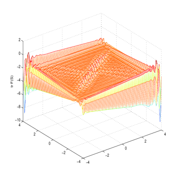
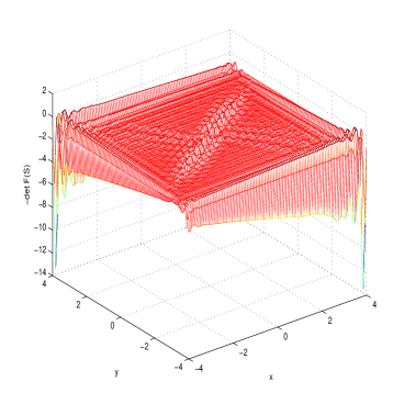
Fig. 1: Left: $\mathop{\mathrm{tr}}\limits F(S)(x,y)$, right: $-\det F(S)(x,y)$. If both functions are negative, then $F(S)(x,y)$ is negative definite.

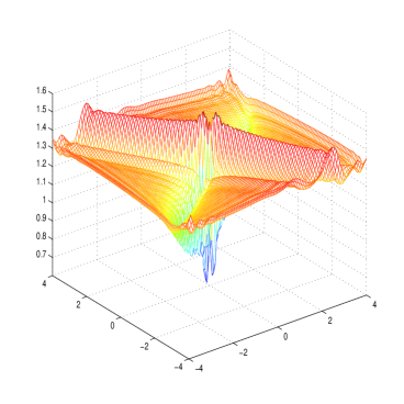
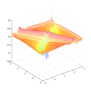
Fig. 2: Left: $\mathop{\mathrm{tr}}\limits S(x,y)$, right: $\det S(x,y)$. If both functions are positive, then $S(x,y)$ is positive definite.

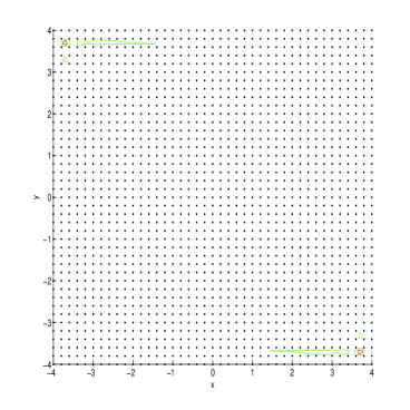
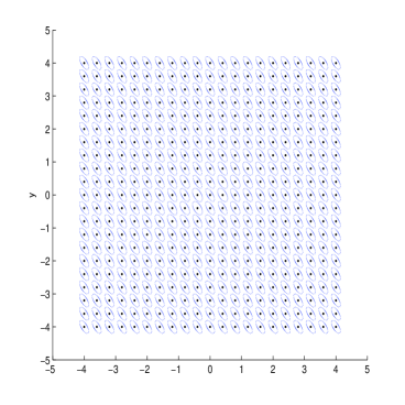
Fig. 3: Left: The points used for the RBF approximation together with the areas where $\mathop{\mathrm{tr}}\limits F(S)(x,y)=0$ (red) and $\det F(S)(x,y)=0$ (green). Right: To illustrate the approximation $S$, around some points ${x}$, we have plotted the curve of equal distance with respect to metric $S({x})$, in particular the set $\{{x}+{v}\mid({v}-{x})^{T}S({x})({v}-{x})={\rm const}\}$.

References

[1]L. Amodei, Reproducing kernels of vector-valued function spaces, in
Surface Fitting and Multiresolution Methods, A. L. Méhaut’e, C. Rabut, and
L. L. Schumaker, eds., Nashville, 1997, Vanderbilt University Press,
pp. 17–26.
[2]N. Aronszajn, Theory of reproducing kernels, Trans. Am. Math. Soc., 68 (1950), pp. 337–404.
[3]E. M. Aylward, P. A. Parrilo, and J.-J. Slotine, Stability and
robustness analysis of nonlinear systems via contraction metrics and SOS
programming, Automatica, 44 (2008), pp. 2163–2170.
[4]M. N. Benbourhim and A. Bouhamidi, Meshless pseudo-polyharmonic
divergence-free and curl-free vector fields approximation, SIAM J. Math. Anal., 42 (2010), pp. 1218–1245.
[5]A. Berlinet and C. Thomas-Agnan, Reproducing Kernel Hilbert Spaces
in Probability and Statistics, Springer, New York, 2004.
[6]G. Borg, A condition for the existence of orbitally stable solutions
of dynamical systems, vol. 153 of Kungl. Tekn. Högsk. Handl., Elander,
1960.
[7]M. D. Buhmann, Radial Basis Functions, Cambridge Monographs on
Applied and Computational Mathematics, Cambridge University Press, Cambridge,
2003.
[8]N. Cristianini and J. Shawe-Taylor, An introduction to support
vector machines and other kernel-based learning methods, Cambridge
University Press, Cambridge, 2000.
[9]F. Cucker and S. Smale, On the mathematical foundation of learning,
Bull. Amer. Math. Soc., 39 (2002), pp. 1–49.
[10]J. Dick, F. Y. Kuo, and I. H. Sloan, High-dimensional integration:
The quasi-Monte Carlo way, in Acta Numerica, A. Iserles, ed., vol. 22,
Cambridge University Press, 2013, pp. 133–288.
[11]G. Fasshauer, Meshfree Approximation Methods with MATLAB, World
Scientific Publishers, Singapore, 2007.
[12]N. Flyer and B. Fornberg, Radial basis functions: Developments and
applications to planetary scale flows, Computers and Fluids, 46 (2011),
pp. 23–32.
[13]B. Fornberg and N. Flyer, Solving PDEs with radial basis
functions, in Acta Numerica, A. Iserles, ed., vol. 24, Cambridge University
Press, 2015, pp. 215–258.
[14]F. Forni and R. Sepulchre, A differential Lyapunov framework for
contraction analysis, IEEE Transactions on Automatic Control, 59 (2014),
pp. 614–628.
[15]C. Franke and R. Schaback, Convergence order estimates of meshless
collocation methods using radial basis functions, Adv. Comput. Math., 8
(1998), pp. 381–399.
[16]E. Fuselier, Sobolev-type approximation rates for divergence-free
and curl-free RBF interpolants, Math. Comput., 77 (2008), pp. 1407–1423.
[17]P. Giesl, Construction of global Lyapunov functions using radial
basis functions, vol. 1904 of Lecture Notes in Mathematics, Springer-Verlag,
Heidelberg, 2007.
[18], Converse theorems on
contraction metrics for an equilibrium, J. Math. Anal. Appl., 424 (2015),
pp. 1380–1403.
[19]P. Giesl and S. Hafstein, Construction of a CPA contraction metric
for periodic orbits using semidefinite optimization, Nonlinear Anal., 86
(2013), pp. 114–134.
[20]P. Giesl and S. Hafstein, Computation and verification of Lyapunov
functions, SIAM J. Appl. Dyn. Syst., 14 (2015), p. 1663–1698.
[21], Review on
computational methods for Lyapunov functions, Discrete and Continuous
Dynamical Systems - Series B (DCDS-B), 20 (2015), pp. 2291 – 2331.
[22]P. Giesl and H. Wendland, Meshless collocation: Error estimates with
application to dynamical systems, SIAM J. Numer. Anal., 45 (2007),
pp. 1723–1741.
[23], Construction of a
contraction metric by meshless collocation.
Preprint Bayreuth/Sussex, 2016.
[24]W. Hahn, Stability of Motion, Springer, Berlin, 1967.
[25]P. Hartman, Ordinary Differential Equations, Wiley, New York, 1964.
[26]E. J. Kansa, Multiquadrics - A scattered data approximation scheme
with applications to computational fluid-dynamics I. Surface
approximations and partial derivative estimates, Comput. Math. Appl., 19
(1990), pp. 127–145.
[27]H. Khalil, Nonlinear systems, Macmillan Publishing Company, New
York, 1992.
[28]N. N. Krasovskii, Problems of the Theory of Stability of Motion,
Mir, Moscow, 1959.
[29]G. A. Leonov, I. M. Burkin, and A. I.Shepelyavyi, Frequency Methods
in Oscillation Theory, vol. 357 of Ser. Math. and its Appl., Kluwer, 1996.
[30]S. Lowitzsch, Approximation and Interpolation Employing
Divergence-Free Radial Basis Functions with Applications, PhD thesis, Texas
A&M University, College Station, USA, 2002.
[31]C. A. Micchelli and M. Pontil, Learning the kernel function via
regularization, J. of Mach. Learning Research, 6 (2005), pp. 1099–1125.
[32]F. J. Narcowich and J. D. Ward, Generalized Hermite interpolation
via matrix-valued conditionally positive definite functions, Math. Comput.,
63 (1994), pp. 661–687.
[33]F. J. Narcowich, J. D. Ward, and H. Wendland, Sobolev bounds on
functions with scattered zeros, with applications to radial basis function
surface fitting, Math. Comput., 74 (2005), pp. 643–763.
[34]R. Schaback, The missing Wendland functions, Adv. Comput. Math., 34 (2011), pp. 67–81.
[35]R. Schaback and H. Wendland, Kernel techniques: From machine
learning to meshless methods, in Acta Numerica, A. Iserles, ed., vol. 15,
Cambridge University Press, 2006, pp. 543–639.
[36]B. Schölkopf and A. J. Smola, Learning with Kernels – Support
Vector Machines, Regularization, Optimization, and Beyond, MIT Press,
Cambridge, Massachusetts, 2002.
[37]I. Steinwart and A. Christmann, Support Vector Machines, Springer,
2008.
[38]B. Stenström, Dynamical systems with a certain local contraction
property, Math. Scand., 11 (1962), pp. 151–155.
[39]V. Vapnik, Statistical Learning Theory, John Wiley and Sons, 1998.
[40]H. Wendland, Piecewise polynomial, positive definite and compactly
supported radial functions of minimal degree, Adv. Comput. Math., 4
(1995), pp. 389–396.
[41], Meshless Galerkin
methods using radial basis functions, Math. Comput., 68 (1999),
pp. 1521–1531.
[42], Scattered Data
Approximation, Cambridge Monographs on Applied and Computational
Mathematics, Cambridge University Press, Cambridge, UK, 2005.
[43], Divergence-free
kernel methods for approximating the Stokes problem, SIAM J. Numer. Anal., 47 (2009), pp. 3158–3179.