Abstract

This paper describes the calculation of the next-to-leading order (NLO) QCD corrections to massive color-octet vector boson pair production at hadron colliders. As a concrete framework, a two-site coloron model with an internal parity is chosen, which can be regarded as an effective low-energy approximation of Kaluza-Klein gluon physics in universal extra dimensions. The renormalization procedure involves several subtleties, which are discussed in detail. The impact of the NLO corrections is relatively modest, amounting to a reduction of 11–14% in the total cross-section, but they significantly reduce the scale dependence of the LO result.

1 Introduction

Massive color-octet vector bosons appear in a number of beyond-the-Standard-Model (BSM) theories, such as universal extra dimensions (UED) [1, 2], topcolor models [3], coloron models [4], and moose models [5]. They may be copiously produced at the Large Hadron Collider (LHC), leading to distinct signatures [6] that are actively searched for [7, 8]. Most of these analyses consider single resonance production of the massive octet vectors, with decays into dijet or top-pair final states.

On the other hand, single production of massive color-octet vector bosons is forbidden or suppressed in UED models with Kaluza-Klein (KK) parity or in moose models with a $\mathbb{Z}_{2}$ exchange symmetry, so that pair production becomes the leading production process. The phenomenology of these particles at the LHC has been studied extensively, see for example Ref. [2, 9]. However, these analyses were based on tree-level predictions for the relevant production cross-sections, which are subject to large uncertainties from QCD radiative corrections.

QCD corrections have been computed for a number of pair production processes of colored BSM particles, including (but not limited to) squark and gluino production in the Minimal Supersymmetric Standard Model (MSSM) [10, 11, 12], leptoquark pair production [13], production of massive vector quarks [14], and pair production of scalar color-octet bosons [15]. The corrections were generically found to be sizeable and important to reduce the large dependence of tree-level results on the renormalization scale. Thus, for a robust prediction of the production of colored BSM particles at hadron colliders, the inclusion of next-to-leading order (NLO) QCD corrections is mandatory.

QCD corrections to production of single vector octets have been studied in Refs. [16, 17]. In this paper, we consider pair production of massive color-octet vector bosons at hadron colliders at NLO precision. For concreteness, the calculation is based on a two-site coloron model with exchange symmetry. This model can be regarded as a low-energy effective theory of minimal UED with one extra dimension (mUED), which includes only the first KK level as dynamic degrees of freedom. In contrast to new colored scalars or fermions, the analysis of colored vector bosons involves several subtleties concerning the gauge fixing and the renormalization procedure. In particular, there is an inherent ambiguity in the definition of the coupling renormalization. This is a reflection of the fact that the two-site model is manifestly non-renormalizable and thus depends on assumptions about the ultra-violet (UV) completion. This issue will be discussed in some detail in the following, before presenting the technical aspects of the calculation and the numerical results.

The paper is organized as follows: In the next section, the two-site coloron model is introduced, including a detailed description of the role of the exchange symmetry, which is reminiscent of KK-parity in mUED. Section 3 discusses the calculation of the NLO corrections to coloron pair production. Special emphasis is placed on the renormalization procedure and the treatment of infra-red (IR) divergencies through phase-space slicing. In section 4, numerical results for the total cross-section and the rapidity distribution are shown, before concluding in section 5. For the reader’s convenience, the Feynman rules of the two-site coloron model are provided in the appendix.

2 The two-site symmetric coloron model

The two-site coloron model is based on an extension of the strong gauge group to the product group $\text{SU(3)}_{1}\times\text{SU(3)}_{2}$, which is broken down to $\text{SU(3)}_{\rm C}$ by a non-linear sigma model. In addition, invariance under the $\mathbb{Z}_{2}$ transformation $\cal P$ is imposed, which interchanges the two SU(3) groups:

$${\cal P}:\quad\text{SU(3)}_{1}\leftrightarrow\text{SU(3)}_{2}.$$ (1)

This exchange symmetry mimics the KK parity of UED. The Lagrangian of the model can be divided into three parts,

$${\cal L}={\cal L}_{\rm gauge}+{\cal L}_{\rm ferm}+{\cal L}_{\rm gf}.$$ (2)

The gauge part is given by

$${\cal L}_{\rm gauge}=-\frac{1}{4}G_{1\mu\nu}G_{1}^{\mu\nu}-\frac{1}{4}G_{2\mu\nu}G_{2}^{\mu\nu}+\frac{f^{2}}{4}\,\text{tr}\{D_{\mu}\Sigma D^{\mu}\Sigma^{\dagger}\}.$$ (3)

Here $G_{i\mu\nu}$ are the field strength tensors of SU(3)_i ($i=1,2$), with gauge couplings $g_{1}=g_{2}\equiv g$. $\Sigma$ denotes the non-linear sigma field

$$\Sigma=\exp(2i\pi^{A}T^{A}/f),$$ (4)

where $A=1,...,8$ is implicitly summed over, $T^{A}$ are the SU(3) generators, $f$ is a constant of mass dimension, and $\pi^{A}$ are the Goldstone fields of the broken SU(3). Its covariant derivative is given by

$$D_{\mu}\Sigma=\partial_{\mu}\Sigma-ig\,G^{A}_{1\mu}T^{A}\Sigma+ig\,\Sigma G^{A}_{2\mu}T^{A}.$$ (5)

Under $\text{SU(3)}_{1}\times\text{SU(3)}_{2}$, the $\Sigma$ field transforms as a bi-fundamental,

$$\Sigma\to U_{1}\,\Sigma\,U_{2}^{\dagger}.$$ (6)

The $\Sigma$ field is responsible for the breaking of $\text{SU(3)}_{1}\times\text{SU(3)}_{2}$ to the vectorial subgroup $\text{SU(3)}_{\rm C}$. The gauge mass eigenstates in the broken phase are

$$G^{A}_{\mu} =\tfrac{1}{\sqrt{2}}(G^{A}_{1\mu}+G^{A}_{2\mu}), C^{A}_{\mu} =\tfrac{1}{\sqrt{2}}(G^{A}_{1\mu}-G^{A}_{2\mu}).$$ (7)

Here $G^{A}_{\mu}$ is the (massless) gluon field of $\text{SU(3)}_{\rm C}$ with coupling strength $g_{\rm s}=g/\sqrt{2}$, whereas $C^{A}_{\mu}$ is the massive coloron field with mass $M=g_{\rm s}f$, which “eats” the Goldstone fields $\pi^{A}$.

Eq. (3) has the same form as for the coloron model in Ref. [16] with the additional constraint that the two gauge groups have equal coupling strength. The latter requirement is a consequence of the $\cal P$ parity, which was not considered in Ref. [16]. Under this parity

$${\cal P}:\quad G_{1\mu}^{A} \leftrightarrow G_{2\mu}^{A}, G_{\mu}^{A} \to G_{\mu}^{A}, C_{\mu}^{A} \to-C_{\mu}^{A}, \Sigma \to\Sigma^{\dagger}.$$ (8)

Since $C^{A}_{\mu}$ is odd under $\cal P$, the massive colorons can only be produced in pairs.

The fermion part of the Lagrangian reads

$${\cal L}_{\rm ferm}={} \bar{q}_{1}i\cancel{D}_{1}q_{1}+\bar{q}_{2}i\cancel{D}_{2}q_{2}+\bar{q}^{\prime}i\cancel{D}_{\rm V}q^{\prime}-Y\bigl{[}\bar{q}_{1}\xi q^{\prime}-\bar{q}_{2}\xi^{\dagger}q^{\prime}+\text{h.c.}\bigr{]}$$

$$+\bar{u}_{1}i\cancel{D}_{1}u_{1}+\bar{u}_{2}i\cancel{D}_{2}u_{2}+\bar{u}^{\prime}i\cancel{D}_{\rm V}u^{\prime}-Y\bigl{[}\bar{u}_{1}\xi u^{\prime}-\bar{u}_{2}\xi^{\dagger}u^{\prime}+\text{h.c.}\bigr{]}$$ (9)

$$+\bar{d}_{1}i\cancel{D}_{1}d_{1}+\bar{d}_{2}i\cancel{D}_{2}d_{2}+\bar{d}^{\prime}i\cancel{D}_{\rm V}d^{\prime}-Y\bigl{[}\bar{d}_{1}\xi d^{\prime}-\bar{d}_{2}\xi^{\dagger}d^{\prime}+\text{h.c.}\bigr{]}.$$

Here $\psi_{1}$, $\psi_{2}$ and $\psi^{\prime}$ are quark fields in the fundamental representation of SU(3)₁, SU(3)₂ and SU(3)_C, respectively ($\psi=q,u,d$). The $\psi=q$ fields are chiral doublets under the weak SU(2)_W group, whereas $\psi=u,d$ are singlets. The relevant quantum numbers and chirality of the quark fields is summarized in Tab. 1.

Field	Chirality	SU(2)W	SU(3)1	SU(3)2	SU(3)C
$q_{1}$	L	2	3	1	–
$q_{2}$	L	2	1	3	–
$q^{\prime}$	R	2	–	–	3
$u_{1}$	R	1	3	1	–
$u_{2}$	R	1	1	3	–
$u^{\prime}$	L	1	–	–	3
$d_{1}$	R	1	3	1	–
$d_{2}$	R	1	1	3	–
$d^{\prime}$	L	1	–	–	3

Table 1: Quantum numbers and chirality of the quark fields in the two-site symmetric coloron model.

Their covariant derivatives read

$$D_{1\mu}\psi_{1} =\partial_{\mu}\psi_{1}-igG^{A}_{1\mu}T^{A}\psi_{1}+...,$$

$$D_{1\mu}\psi_{2} =\partial_{\mu}\psi_{2}-igG^{A}_{2\mu}T^{A}\psi_{2}+..., [\psi=q,u,d]$$

$$D_{\rm V\mu}\psi^{\prime} =\partial_{\mu}\psi^{\prime}-\tfrac{ig}{\sqrt{2}}(G^{A}_{1\mu}+G^{A}_{2\mu})T^{A}\psi^{\prime}+...,$$ (10)

where the dots indicate electroweak interactions, which are ignored in this work. Furthermore, $\xi$ is the “square root” sigma field according to the CCWZ construction [18],

$$\xi=\exp(i\pi^{A}T^{A}/f).$$ (11)

Under $\text{SU(3)}_{1}\times\text{SU(3)}_{2}$, these fields transform as

$$\psi_{1} \to U_{1}\psi_{1}, \psi_{2} \to U_{2}\psi_{2}, \psi^{\prime} \to U_{\rm V}\psi^{\prime}, \xi\to U_{1}\xi U_{\rm V}^{\dagger}=U_{\rm V}\xi U_{2}^{\dagger},$$ (12)

where $U_{\rm V}$ is the transformation matrix of the fundamental representation of the vectorial subgroup SU(3)_C. The effect of $\cal P$ parity on the fermion fields is

$${\cal P}:\quad\psi_{1} \leftrightarrow\psi_{2}, \psi^{\prime} \to-\psi^{\prime}, \xi \to\xi^{\dagger}.$$ (13)

The introduction of the $\psi^{\prime}$ fields is necessary to be able to write down invariant Yukawa terms (with coupling strength $Y$) in eq. (9).

The physical quark mass eigenstates are

$$\psi =\tfrac{1}{\sqrt{2}}(\psi_{1}+\psi_{2}), [\psi=q,u,d]$$

$$\Psi =\tfrac{1}{\sqrt{2}}(\psi_{1}-\psi_{2})P_{L}+\psi^{\prime}P_{R}, [\Psi=Q,U,D]$$ (14)

where $P_{L,R}=\frac{1}{2}(1\pm\gamma_{5})$. Here the $\psi$ fields are massless chiral $\cal P$-even SM-like quark fields, whereas the $\Psi$ fields are $\cal P$-odd fermion fields with a vector-like mass $M_{\Psi}=\sqrt{2}Y$. In general, the Yukawa coupling $Y$ is a free parameter, but for the sake of analogy to UED we impose

$$Y=M/\sqrt{2},\quad\text{i.e.}\quad M_{\Psi}=M.$$ (15)

For the top quark, the SM Higgs Yukawa coupling cannot be ignored. It leads to mixing between the $U_{3}$ and first component of the $Q_{3}$ fields, where the subscript indicates the generation index, see e.g. App. H of Ref. [19]. The mass matrix reads

$$\begin{pmatrix}\overline{Q}_{3}&\overline{U}_{3}\end{pmatrix}\begin{pmatrix}M&m_{t}\\ m_{t}&-M\end{pmatrix}\begin{pmatrix}Q_{3}\\ U_{3}\end{pmatrix},$$ (16)

leading to two degenerate mass eigenstates $T$ and $T^{\prime}$ given by

$$\begin{pmatrix}Q_{3}\\ U_{3}\end{pmatrix}=\begin{pmatrix}\cos\theta_{T}&\gamma_{5}\sin\theta_{T}\\ \sin\theta_{T}&-\gamma_{5}\cos\theta_{T}\end{pmatrix}\begin{pmatrix}T\\ T^{\prime}\end{pmatrix}$$ (17)

with mass and mixing angle

$$M_{T} =\sqrt{M^{2}+m_{t}^{2}}, \tan 2\theta_{T} =\frac{m_{t}}{M}.$$ (18)

The final component of the model is the gauge-fixing and ghost term. For a covariant gauge it can be defined in the following $\cal P$-symmetric form,

$${\cal L}_{\rm gf} =-\tfrac{1}{2}({\cal F}_{1}^{A})^{2}-\tfrac{1}{2}({\cal F}_{2}^{A})^{2}+\sum_{i,j=1}^{2}\bar{u}^{A}_{i}\frac{\delta{\cal F}^{A}_{i}}{\delta\alpha^{B}_{j}}u^{B}_{j},$$ (19)

where

$${\cal F}_{1}^{A} =\frac{1}{\sqrt{\xi}}G^{A}_{1\mu}+\sqrt{\xi}\frac{g}{2}f\,\pi^{A},$$

$${\cal F}_{2}^{A} =\frac{1}{\sqrt{\xi}}G^{A}_{2\mu}-\sqrt{\xi}\frac{g}{2}f\,\pi^{A},$$ (20)

and $\delta\alpha^{A}_{i}$ is the parameter of an infinitesimal SU(3)_i gauge transformation. For the calculation presented in the following sections, the Feynman gauge $\xi=1$ has been employed. In this gauge, the unphysical Goldstone fields $\pi^{A}$ receive a mass $M=g_{\rm s}f=gf/\sqrt{2}$ from eq. (19). The ghost fields mix to form a $\cal P$-even massless gluon ghost $u_{g}=\frac{1}{\sqrt{2}}(u_{1}+u_{2})$ and a $\cal P$-odd coloron ghost $u_{C}=\frac{1}{\sqrt{2}}(u_{1}+u_{2})$ with mass $M$. Thus one obtains

$${\cal L}_{\rm gf}= {}-\frac{1}{2}\Bigl{[}(\partial^{\mu}G_{\mu}^{A})^{2}+(\partial^{\mu}C_{\mu}^{A})^{2}\Bigr{]}-\frac{M^{2}}{2}(\pi^{A})^{2}-M\,\partial^{\mu}C_{\mu}^{A}\,\pi^{A}$$

$$-\bar{u}^{A}_{g}\partial^{2}u^{A}_{g}-\bar{u}^{A}_{C}(\partial^{2}+M^{2})u^{A}_{C}+g_{\rm s}f_{ABC}\,\bar{u}_{g}^{A}\partial^{\mu}(u_{g}^{B}G_{\mu}^{C}+u_{C}^{B}C_{\mu}^{C})$$

$$+g_{\rm s}f_{ABC}\,\bar{u}_{C}^{A}\partial^{\mu}(u_{g}^{B}C_{\mu}^{C}+u_{C}^{B}G_{\mu}^{C})+g_{\rm s}Mf_{ABC}(\bar{u}^{A}_{g}u^{B}_{C}-\bar{u}^{A}_{C}u^{B}_{g})\pi^{C}.$$ (21)

In summary, the two-site symmetric coloron model defined in this way contains several states with mass $M$ in addition to the SM particle content. Besides the coloron vector-boson, heavy vector-like quarks are required to enforce the $\cal P$-parity as an exact symmetry.

This model can be viewed as a low-energy approximation of the 5-dimensional minimal UED model (mUED) with compactification radius $R=M^{-1}$, where only the zero modes and first KK excitations are kept as dynamical degrees of freedom. Note, however, that the coloron model is not identical to a simple truncation of mUED at the $N_{\rm KK}=1$ level, since such a truncated UED model would violate gauge invariance [20], whereas the model presented here respects the full gauge symmetry, albeit non-linearly. In fact, the Feynman rules for the two-site coloron model and the first KK excitation in mUED are mostly identical, but there are a few differences, which are mentioned in appendix A.

In a more general sense, the two-site symmetric coloron model can be regarded as a low-energy description of any model with massive color-octet vector bosons that are odd under some (approximate) parity.

3 NLO corrections to the pair production process

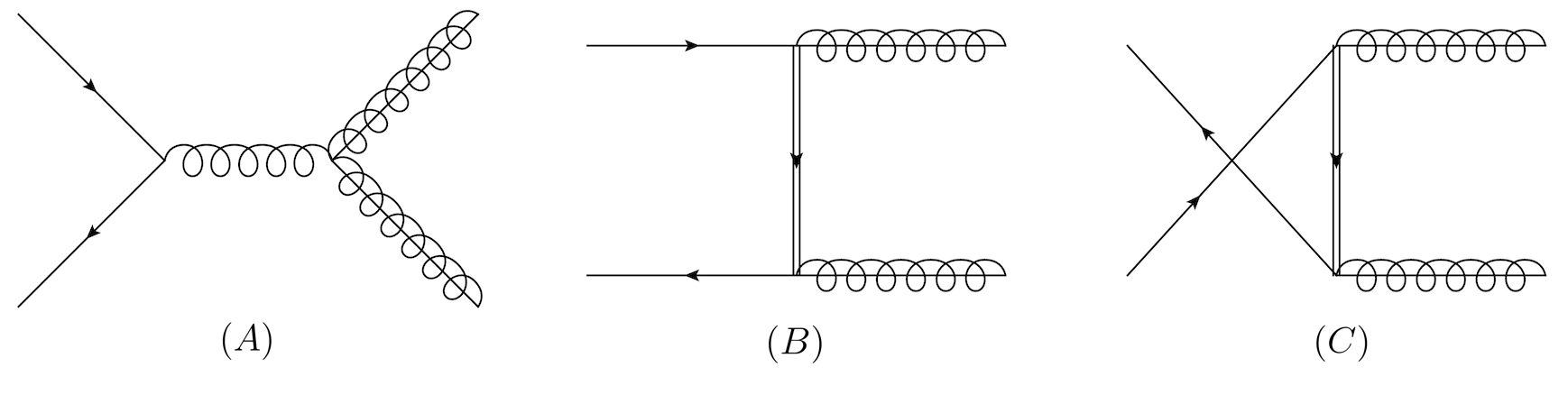
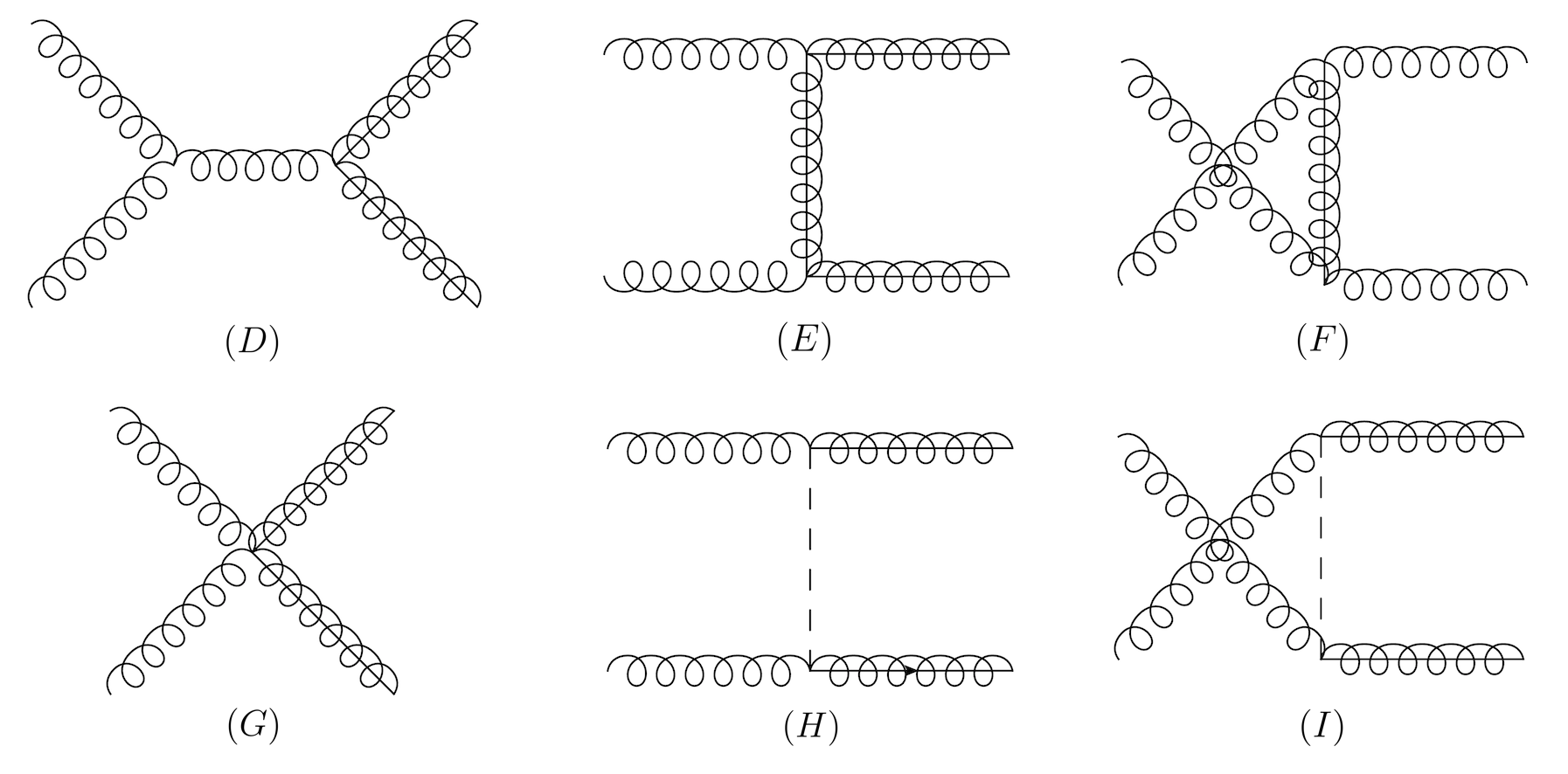
Figure 1: Born-level diagrams contributing to massive color-octet vector-boson pair production. Here the spring–solid lines indicate massive color-octet vector-bosons, while the double lines indicate massive $\cal P$-odd quarks, and the dashed line indicates a $\cal P$-odd Goldstone scalar.

Massive colorons can be pair produced at hadron colliders, such as the LHC. The tree-level process $pp\to CC$ can be divided into two partonic sub-channels, $q\bar{q}\to CC$ and $gg\to CC$, with the relevant diagrams shown in Fig. 1. Note that at leading order this process is identical to of KK gluon pair production in mUED.

At NLO, one needs to consider one-loop corrections to the subprocesses $q\bar{q}\to CC$ and $gg\to CC$, as well as real emission of an extra gluon at tree-level, $q\bar{q}\to CCg$ and $gg\to CCg$. A few sample diagrams are shown in Figs. 2 and 3. Both the loop contributions and real emission contributions are separately IR divergent, but the divergencies cancel in the combined result. Additionally, the quark-gluon induced subprocesses $qg\to CCq$ and $\bar{q}g\to CC\bar{q}$ appear for the first time at NLO.

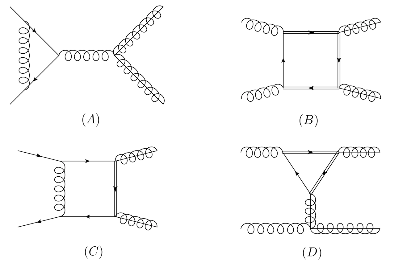
Figure 2: Sample one-loop diagrams contributing to coloron pair production. See Fig. 1 for the definition of the different propagator line types.

Figure 3: Sample real radiation diagrams contributing to coloron pair production. See Fig. 1 for the definition of the different propagator line types.

At NLO, the predictions for coloron pair production become sensitive to assumptions about the UV completion. The renormalization procedure employed here takes a bottom-up approach, assuming that the running couplings are defined at the mass scale $M$ of the colorons. In the next subsection, the renormalization scheme is discussed in more detail.

3.1 Renormalization

In this work, the renormalization is performed by using the on-shell scheme for the wave-function and mass renormalization of the physical states and $\overline{\text{MS}}$ renormalization for the strong coupling constant. However, due to the fact that the two-site coloron model is fundamentally a non-renormalizable theory, there are several subtleties that need to be addressed. These will be discussed in this section, together with a brief summary of the remaining aspects of the renormalization.

For the external states the wave-function renormalization constants

$$\delta Z^{\psi}_{\rm L}=\delta Z^{\psi}_{\rm R}\quad[\psi=q,u,d],\qquad\delta Z^{g},\qquad\delta Z^{C}$$ (22)

are introduced for the left- and right-handed (massless) SM quarks, the gluons, and the massive colorons, respectively. As usual, their values are determines through the residues of the renormalized propagators, leading to

$$\delta Z^{\psi}_{\rm L,R} =-{\Re\rm e}\{\Sigma^{\psi}_{\rm L,R}(0)\}, \delta Z^{g} =-{\Re\rm e}\bigl{\{}\tfrac{\partial}{\partial(p^{2})}\Sigma^{g}(0)\bigr{\}}, \delta Z^{C} =-{\Re\rm e}\bigl{\{}\tfrac{\partial}{\partial(p^{2})}\Sigma^{C}(M^{2})\bigr{\}},$$ (23)

where $\Sigma^{\psi}_{\rm L,R}(p^{2})$, $\Sigma^{g}(p^{2})$ and $\Sigma^{C}(p^{2})$ are the left/right-handed quark self-energies, transverse gluon self-energy and transverse coloron self-energy, respectively.

The masses of the colorons and massive quarks are renormalized according to the on-shell prescriptions

$$\delta M_{C}^{2} ={\Re\rm e}\{\Sigma^{C}(M^{2})\}, \delta M_{\Psi} =\frac{M}{2}{\Re\rm e}\bigl{\{}\Sigma^{\psi}_{\rm L}(M^{2})+\Sigma^{\psi}_{\rm R}(M^{2})+2\Sigma^{\psi}_{\rm S}(M^{2})\bigr{\}}.$$ (24)

The mass parameter in the gauge-fixing term gets renormalized in the same way as the coloron mass. Note that, while we assume that the colorons and massive quarks have the same mass $M$ at tree-level, as in mUED, they are technically independent parameters in the coloron model and thus receive different mass counterterms. In mUED, in fact, the degeneracy of the KK masses is also broken at the one-loop level due to boundary terms [21].

Following the analogy to mUED, therefore, we assume that the mass difference between the coloron mass, $M_{C}$, and the vector-like quark mass, $M_{\Psi}$, is small: $|M_{C}-M_{\Psi}|/M\sim{\cal O}(\alpha_{\rm s})$. Within the contributions to ${\cal O}(\alpha_{\rm s})$ we thus set $M_{C}=M_{\Psi}=M$ but allow the masses to deviate by a small numerical amount in the tree-level contribution, consistent with this power counting.

The strong coupling constant is renormalized in the 5-flavor $\overline{\text{MS}}$ scheme. In this scheme, only the gluons and five light quarks are included in the scale evolution of the $\alpha_{\rm s}$, whereas the scale dependence of the top quark, coloron and heavy vector quark loops is accounted for through explicit logarithms in the finite part of the counterterm. See e.g. Ref. [10] for an application of this scheme in the context of supersymmetry. For the $g\psi\bar{\psi}$, $ggg$, $g\Psi\bar{\Psi}$ and $gCC$ gauge coupling, this leads to

$$g_{\rm s}^{\rm bare}\to g_{\rm s}(\mu)\,\bigl{(}1+\delta Z_{g}\bigr{)}$$ (25)

$$\begin{aligned} \delta Z_{g}=\frac{\alpha_{\rm s}(\mu)}{4\pi}\biggl{[}\!&-\frac{\beta_{0}}{2}\biggl{(}\frac{1}{\epsilon}-\gamma_{\rm E}+\log(4\pi)\biggr{)}\\ &-\frac{1}{3}\log\frac{m_{t}^{2}}{\mu^{2}}+\biggl{(}\frac{21}{4}-\frac{2}{3}n_{q}\biggr{)}\log\frac{M^{2}}{\mu^{2}}-\frac{2}{3}\log\frac{M_{T}^{2}}{\mu^{2}}\biggr{]},\end{aligned}$$ (26)

$$\beta_{0}=\beta_{0}^{\rm L}+\beta_{0}^{\rm H}=\Bigl{(}11-\frac{2}{3}n_{q}\Bigr{)}+\Bigl{(}\frac{21}{2}-\frac{4n_{q}+6}{3}\Bigr{)},$$ (27)

where $n_{q}=5$, and $\mu$ is the renormalization scale, which is taken equal to the regularization scale for simplicity. Furthermore, $\epsilon=(4-d)/2$, where $d$ is the number of dimensions in dimensional regularization.

On the other hand, for the $C\psi\Psi$ and $gC\pi$ couplings (where $\pi$ is a Goldstone boson), one needs different coupling counterterms. This is not entirely surprising, since these couplings are not SU(3)_C gauge interactions, but are instead related to the larger non-linear $\text{SU(3)}_{1}\times\text{SU(3)}_{2}$ symmetry.

To determine the $\mu$-dependence of these couplings, one may assume that all gluon and coloron coupling have the same value at $\mu=M$, and the $C\psi\Psi$ and $gC\pi$ couplings do not effectively run for $\mu<M$. Thus one finds

$$C\psi\Psi: \delta Z^{\prime}_{g}=\frac{\alpha_{\rm s}(\mu)}{4\pi}\biggl{[}-\biggl{(}10-\frac{2}{3}n_{q}\biggr{)}\biggl{(}\frac{1}{\epsilon}-\gamma_{\rm E}+\log(4\pi)\biggr{)}+\frac{\beta_{0}^{\rm L}}{2}\log\frac{M^{2}}{\mu^{2}}\biggr{]},$$ (28)

$$gC\pi: \delta Z^{\prime\prime}_{g}=\frac{\alpha_{\rm s}(\mu)}{4\pi}\biggl{[}-\biggl{(}\frac{21}{4}-\frac{n_{q}}{2}\biggr{)}\biggl{(}\frac{1}{\epsilon}-\gamma_{\rm E}+\log(4\pi)\biggr{)}+\frac{\beta_{0}^{\rm L}}{2}\log\frac{M^{2}}{\mu^{2}}\biggr{]}.$$ (29)

In addition, one needs a counterterm for the vacuum expectation value of the sigma field, $\Sigma$. This counterterm, denoted by the symbol $\delta t$, appears in the renormalization of the Goldstone self-energy:

$$\includegraphics[width=65.04256pt]{counterterm2.png}\;=i\delta_{AB}\frac{\delta t}{M}.$$ (30)

In a Higgs-like theory, this counterterm is usually determined from the requirement that the renormalized tadpole terms of the Higgs field should vanish. For the coloron model, however, the symmetry breaking mechanism is left unspecified, and the radial degrees of freedom of the sigma field (which correspond to the Higgs scalars in a weakly coupled symmetry breaking sector) are assumed to be integrated out. Therefore the tadpole condition cannot be used here.

On the other hand, as explained for example in Ref. [22], the counterterm for the vacuum expectation also appears in the Goldstone self-energy $\Sigma^{\pi}(p^{2})$. Thus one can impose the renormalization condition

$$\delta t=-M\,\Sigma^{\pi}(0),$$ (31)

which in a Higgs-like theory is completely equivalent to the tadpole condition.

3.2 Cancellation of IR divergencies

The real radiation contributions contain divergencies from soft and collinear gluon emission, which cancel against the corresponding singularities in the virtual loop contributions. To carry out this cancellation explicitly, the phase-space slicing method with two cutoffs is employed here [23]. According to this scheme, the phase space integration of the $2\to 3$ real radiation contribution is split into three categories,

$$\sigma_{2\to 3}=\frac{1}{2s}\int d\Gamma_{3}\,|{\cal M}_{3}|^{2}=\frac{1}{2s}\biggl{[}\int_{\rm S}d\Gamma_{3}\,|{\cal M}_{3}|^{2}+\int_{\rm C}d\Gamma_{3}\,|{\cal M}_{3}|^{2}+\int_{\rm H}d\Gamma_{3}\,|{\cal M}_{3}|^{2}\biggr{]}.$$ (32)

Here $d\Gamma_{3}$ is the three-particle phase-space measure, and ${\cal M}_{3}$ is the $2\to 3$ matrix element. On the right-hand side, “S” indicates the soft region, where the gluon energy is restricted to

$$0\leq E_{g}\leq\delta_{\rm s}\frac{\sqrt{\hat{s}}}{2},$$ (33)

where $\hat{s}$ is the partonic center-of-mass energy. For sufficiently small values of $\delta_{\rm s}$, the soft contribution factorizes into the born matrix element and an eikonal factor,

$$\int_{\rm S}d\Gamma_{3}\,|{\cal M}_{3}|^{2} =\int d\Gamma_{2}\,|{\cal M}_{2}|^{2}\times\frac{\alpha_{\rm s}}{2\pi}\,\frac{\Gamma(1-\epsilon)}{\Gamma(1-2\epsilon)}\Bigl{(}\frac{4\pi\mu_{\rm R}^{2}}{s}\Bigr{)}^{\epsilon}\sum_{i,j}\int d\Gamma_{g}\,\frac{-p_{i}\cdot p_{j}}{(p_{i}\cdot p_{g})(p_{j}\cdot p_{g})}\,.$$ (34)

Here $d\Gamma_{2}$ and ${\cal M}_{2}$ are the two-particle phase-space measure and Born matrix element, respectively, while $d\Gamma_{g}$ is the single-particle phase-space measure for the gluon momentum, and the sum $\sum_{i,j}$ runs over all external legs. The eikonal factor can be integrated analytically (see e.g. Refs. [23, 24]).

The label “C” denotes the hard collinear region, defined by

$$\delta_{\rm s}\frac{\sqrt{\hat{s}}}{2}<E_{g}, 1-\cos\theta_{gi}\leq\delta_{\rm c}\frac{\sqrt{\hat{s}}}{E_{g}},$$ (35)

where $\theta_{gi}$ is the angle between the final-state gluon and the incoming parton $i$ ($i=1,2$). For small $\delta_{\rm c}$, the phase space measure and matrix element factorize into the born contribution and the divergent Altarelli-Parisi splitting kernels. In dimensional regularization one thus obtains

$$\int_{\rm C}d\Gamma_{3}\,|{\cal M}_{3}|^{2} =\int d\Gamma_{2}\,|{\cal M}_{2}|^{2}\times\frac{\alpha_{\rm s}}{2\pi}\,\frac{\Gamma(1-\epsilon)}{\Gamma(1-2\epsilon)}\Bigl{(}\frac{4\pi\mu_{\rm R}^{2}}{s}\Bigr{)}^{\epsilon}\Bigl{(}\frac{A_{1}^{\rm c}}{\epsilon}+A_{0}^{\rm c}\Bigr{)},$$ (36)

where $A_{1}^{\rm c}$ and $A_{0}^{\rm c}$ are known numerical constants (see e.g. Refs. [23]). The collinear divergencies in the splitting functions can be absorbed into the renormalization of the parton distribution functions (PDFs) of the incoming partons. The form of eq. (36) presumes that the $\overline{\text{MS}}$ scheme, with the renormalization scale $\mu_{\rm R}$, is used for this purpose.

The soft and collinear contributions are combined with the virtual corrections to arrive at

$$d\sigma =\sum_{i,j}\int dx_{1}dx_{2}\,\Bigl{\{}\bigl{[}f_{i}(x_{1},\mu_{\rm F})f_{j}(x_{2},\mu_{\rm F})+(1\leftrightarrow 2)\bigr{]}\bigl{[}d\hat{\sigma}^{(0)}_{ij}(\hat{s})+d\hat{\sigma}^{(1)}_{ij}(\hat{s};\delta_{\rm s})\bigr{]}$$

$$\qquad+\bigl{[}\tilde{f}_{i}(x_{1},\mu_{\rm F})f_{j}(x_{2},\mu_{\rm F})+\tilde{f}_{j}(x_{1},\mu_{\rm F})f_{i}(x_{2},\mu_{\rm F})+(1\leftrightarrow 2)\bigr{]}d\hat{\sigma}^{(0)}_{ij}(\hat{s})\Bigr{\}}$$ (37)

with

$$\tilde{f}_{i}(x,\mu_{\rm F}) =\sum_{k}\int_{x}^{1-\delta_{\rm s}}\frac{dz}{z}\;f_{k}\Bigl{(}\frac{x}{z},\mu_{\rm F}\Bigr{)}\,\frac{\alpha_{\rm s}}{2\pi}\biggl{[}P_{ik}(z)\,\ln\biggl{(}\frac{\hat{s}}{\mu_{\rm F}^{2}}\,\frac{1-z}{z}\,\delta_{\rm c}\biggr{)}-P^{\prime}_{ik}(z)\Biggr{]}.$$ (38)

Here $f_{i}(x,\mu_{\rm F})$ is the proton PDF for the parton $i$ with the factorization scale $\mu_{\rm F}$; $d\hat{\sigma}^{(0)}_{ij}$ is the differential partonic Born cross-section for the incoming partons $i$ and $j$; $d\hat{\sigma}^{(0)}_{ij}$ is the one-loop corrected partonic cross-section including the soft radiation terms; $P_{ik}(z)$ and $P^{\prime}_{ik}(z)$ are the finite and ${\cal O}(\epsilon)$ pieces of the unregulated splitting kernels (see e.g. Refs. [23]), and $\hat{s}=x_{1}x_{2}s$. Note that the form of eq. (37) changes slightly for the quark-gluon induced subprocesses, which do not receive Born contributions.

The remaining hard radiation region, labeled “H”, is constrained by the conditions $\delta_{\rm s}\frac{\sqrt{\hat{s}}}{2}<E_{g}$ and $1-\cos\theta_{gi}>\delta_{\rm c}\frac{\sqrt{\hat{s}}}{E_{g}}$. It is finite and can be computed with numerical Monte-Carlo integration methods. Both the hard contribution and the result in eq. (37) separately depend on the choices for $\delta_{\rm s}$ and $\delta_{\rm c}$. However, as long as the cutoff parameters are kept sufficiently small, this dependence drops out in the combined total result.

3.3 Notes on the technical implementation

The calculation has been performed using several publicly available computing tools, but additional components were specifically implemented by the authors. The Feynman rules of the coloron model (see Appendix A) have been incorporated into FeynArts 3 [25], which was used for generating the relevant diagrams and amplitudes. The color, Dirac and Lorentz algebra was performed with FeynCalc [26].

To simplify the treatment of tensor loop integrals, the one-loop amplitude was contracted with the Born amplitude and the sum over the spins of external particles carried out before any tensor reduction. As a result, most tensor structures in the numerator of the loop integrand can be canceled against propagator denominators. For the remaining tensor integrals, Passarino-Veltman reduction has been used [27]. One thus arrives at a final result in terms of standard one-loop basis functions. The IR-finite basis integrals have been evaluated numerically using LoopTools 2 [28], whereas the IR-divergent basis integrals were taken from Ref. [29].

For the $q\bar{q}$ channel, two fully independent calculations have been carried out. One is based on dimensional regularization for the UV singularities and gluon and quark mass regulators for the soft and collinear divergencies, respectively. The other calculation has employed dimensional regularization for all types of singularities. Perfect agreement between the two results at the level of differential cross-sections was obtained. For the $gg$ channel, the use of a mass regulator is not suitable. Nevertheless, we have performed many independent checks of partial contributions to the final result.

The numerical integration over the final-state phase space and initial-state PDFs is implemented in the form of a Monte-Carlo generator in Fortran. This implementation is based on Ref. [30] and produces weighted parton-level events.

4 Numerical results

In the following, we present phenomenological results for coloron pair production at the LHC with $\sqrt{s}=14\,\,\mathrm{TeV}$. Throughout this section, the CTEQ6.1M PDF set [31] have been used, as incorporated in the LHAPDF framework [32].

As a first consistency check, the independence of the total NLO cross-section on the soft and collinear slicing cut-offs, $\delta_{\rm s}$ and $\delta_{\rm c}$ is shown in Fig. 4. The figure depicts two separate plots for the dependence on $\delta_{\rm s}$ and $\delta_{\rm c}$, respectively. It can be seen that the combined virtual, soft and collinear contributions ($\sigma_{\rm S+V}$) and the hard real emission contribution ($\sigma_{2\to 3}$) are separately logarithmically dependent on $\delta_{\rm s}$ and $\delta_{\rm c}$, but this dependence cancels in the sum $\sigma_{\rm NLO}=\sigma_{\rm S+V}+\sigma_{2\to 3}$. The remaining power contributions, proportional to $\delta_{\rm s}^{n}$ and $\delta_{\rm c}^{n}$, are negligibly small for all practical purposes if the cut-off parameters are smaller than about $10^{-3}$ and $10^{-4}$, respectively.

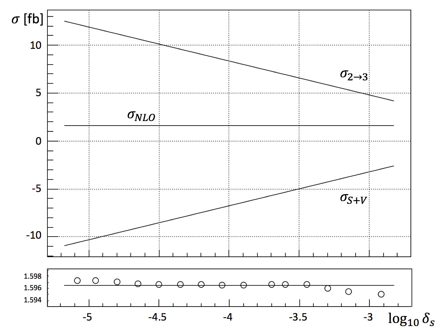
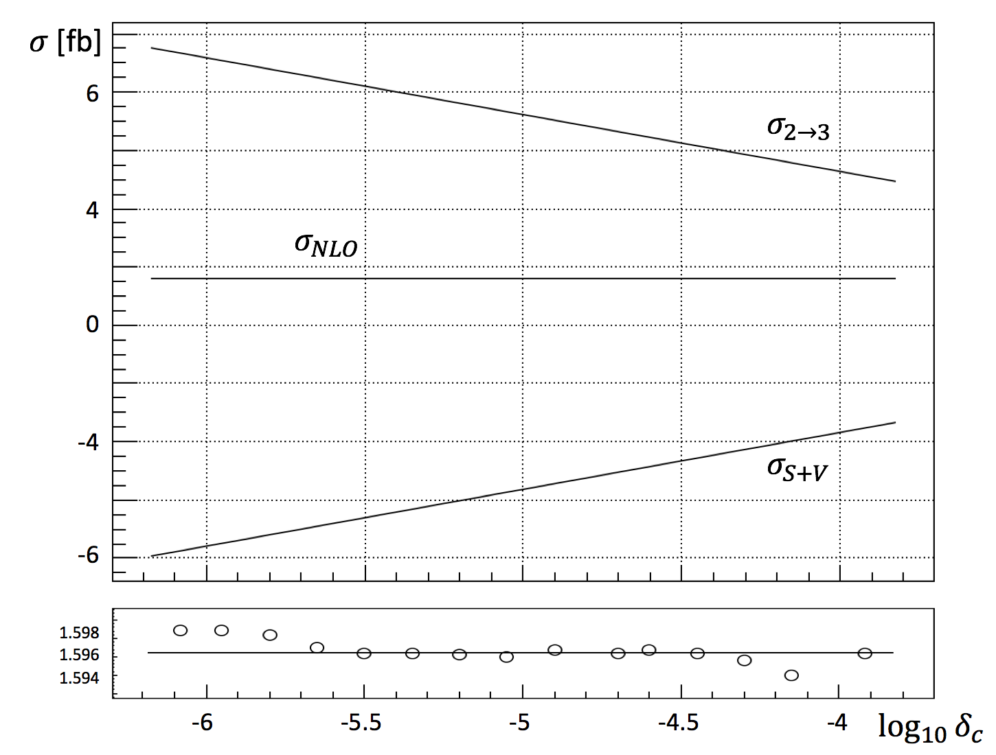
Figure 4: Dependence of the NLO cross-section for the $pp\to CC$ on the soft cut-off $\delta_{\rm s}$ (left) and the collinear cut-off $\delta_{\rm c}$ (right). Both plots are for a $pp$ center-of-mass energy of $\sqrt{s}=14\,\,\mathrm{TeV}$, coloron mass $M=1\,\,\mathrm{TeV}$, and renormalization and factorization scales $\mu=\mu_{\rm F}=M$. Furthermore, in the left (right) panel, the fixed value $\delta_{\rm c}=10^{-5}$ ($\delta_{\rm s}=10^{-3.5}$) has been used.

Note that the plots in Fig. 4 are subject to statistical errors from the Monte-Carlo integration over initial parton momentum fractions and final-state phase space. However, the cancellation of soft and collinear logarithms happens already point-by-point for the fully differential cross-section, after integration over only the one-particle phase-space of the massless final-state parton in $\sigma_{2\to 3}$. Therefore, the accuracy of the cancellation of the $\delta_{\rm s}$ and $\delta_{\rm c}$ dependence is very high, as shown in the lower boxes of the Fig. 4.

The optimal choice of the cut-off parameters needs to strike a balance between two constraints: (i) The non-logarithmic power contributions, proportional to $\delta^{n}_{\rm s,c}$, are minimized by choosing each cut-off parameter as small as possible, whereas (ii) the statistical error for the $2\to 3$ phase-space integration increases if $\delta_{\rm s,c}$ are too small. For the remainder of this section, we use $\delta_{\rm s}=5\times 10^{-4}$ and $\delta_{\rm c}=5\times 10^{-5}$.

In Fig. 5, the LO and NLO total cross-sections are shown as a function of the coloron mass $M$. For this plot, the mass of the $\cal P$-odd quarks has been fixed according to the mUED prediction, i.e. $M_{\Psi}=M-\Delta M$, where $\Delta M$ is the mass splitting due to boundary terms in mUED [21]

$$\Delta M=M\,\frac{11\alpha_{\rm s}}{16\pi}\,\ln\frac{\Lambda^{2}}{\mu^{2}}$$ (39)

Since $\Delta M$ is a one-loop contribution itself, we neglect it inside the ${\cal O}(\alpha_{\rm s})$ corrections to the cross-section and set $M_{\Psi}=M$ there. For the UV cut-off of mUED we choose $\Lambda=20\,M$.

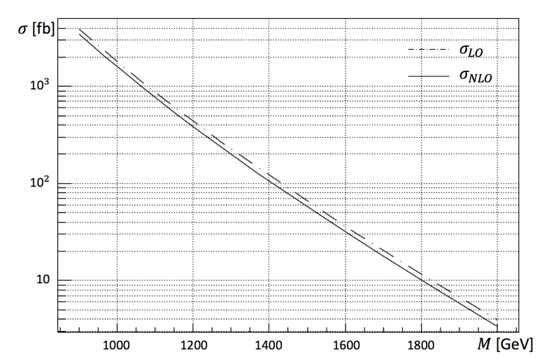
Figure 5: Total LO and NLO coloron pair production cross-sections as function of the coloron mass $M$, for $\sqrt{s}=14\,\,\mathrm{TeV}$ and $\mu=\mu_{\rm F}=M$. The mass splitting between the colorons and $\cal P$-odd quarks has been set to the value predicted by mUED, see text and eq. (39). The lower panel shows the ratio between NLO and LO cross-sections.

In the lower part of the figure, the $K$-factor $\sigma_{\rm NLO}/\sigma_{\rm LO}$ of the NLO and Born cross-sections is shown. As evident from this plot, the $K$-factor depends only mildly on $M$ and amounts to about 0.88. It is interesting to note that the NLO contributions are negative in all three subprocesses, $q\bar{q}\to CC+X$, $gg\to CC+X$, and $qg/\bar{q}g\to CC+X$, the latter of which is only generated by $2\to 3$ real emission diagrams and is turned negative due to the PDF renormalization. While the overall correction is relatively modest, and of a typical magnitude for high-energy QCD processes, it is nevertheless relevant for accurately evaluating current limits and the discovery potential of the LHC for mUED and related models [33].

In addition, the computation of the NLO QCD corrections serves to reduce the theoretical uncertainty from the renormalization and factorization scale dependence. This is demonstrated in Fig. 6, where the two scales have been varied in parallel, $\mu=\mu_{\rm F}$. Considering the range $0.75<\mu/M<1.5$, the LO cross-section changes by about ${}^{+15\%}_{-17\%}$, which is reduced to ${}^{+5\%}_{-8\%}$ for the NLO cross-section. Note that the dominant source of uncertainty stems from the renormalization scale, whereas the factorization scale by itself has a subdominant effect.

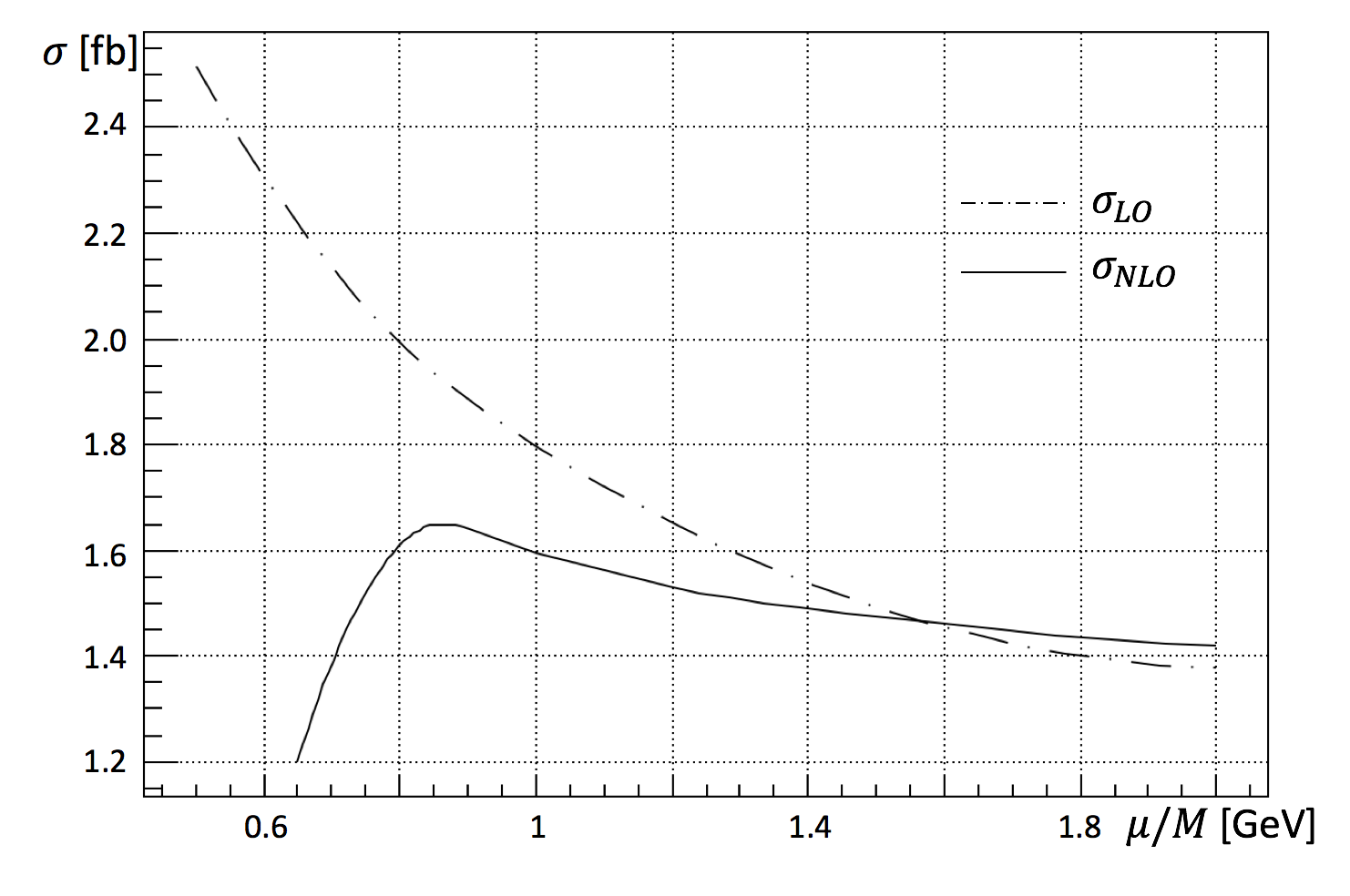
Figure 6: Dependence of the total LO and NLO coloron pair production cross-sections on the combined renormalization and factorization scale $\mu=\mu_{\rm F}$. The plot is based on the $pp$ center-of-mass energy $\sqrt{s}=14\,\,\mathrm{TeV}$, mass $M=1\,\,\mathrm{TeV}$, and mass splitting $M-M_{\Psi}$ as predicted by mUED, see text and eq. (39).

In Fig. 7, we also show how the cross-section changes when the mass splitting $\Delta M=M-M_{\Psi}$ is modified from the mUED prediction. Note that the $gg$ channel does not depend on this parameter at tree-level, and we neglect the mass splitting within the one-loop corrections. Therefore, only the $q\bar{q}$ channel is shown in Fig. 7. We restrict ourselves to the mass ordering $M_{\Psi}<M$, to avoid the situation where the heavy quarks may become resonant in the subprocess $qg\to CCq$, i.e. $qg\to C\Psi$ production with the subsequent decay $\Psi\to Cq$. This would correspond to a different process than than the one studied in this paper and is left for future work. As evident from Fig. 7, the $q\bar{q}\to CC$ subprocess depends very sensitively on $\Delta M$. However, since the $gg$ channel is dominant, the total cross-section varies only by a few percent for reasonable values of the mass splitting.

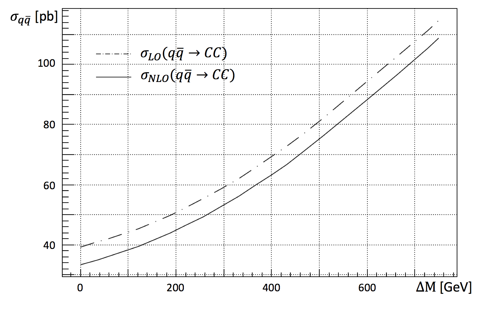
Figure 7: Total LO and NLO coloron pair production cross-sections as function of quark-coloron mass splitting $\Delta M=M-M_{\Psi}$. The other input parameters have been set to $\sqrt{s}=14\,\,\mathrm{TeV}$, mass $M=1\,\,\mathrm{TeV}$, and $\mu=\mu_{\rm F}=M$.

Finally, Fig. 8 displays the impact of the NLO corrections on the differential cross-section in terms of the rapidity $y\equiv\frac{1}{2}\ln\frac{E+p_{\rm L}}{E-p_{\rm L}}$. Here $E$ and $p_{\rm L}$ are the energy and longitudinal momentum of one of the final-state colorons. Since, after summing over colors, we have two identical colorons in the final state, the rapidity distribution is symmetric. As one can see from the figure, the effect of the NLO corrections results in a slight enhancement of the tails of the rapidity distribution relative to the central region. This can be partially understood from a simple kinematic effect, since the recoil against extra radiated partons causes a broadening of the rapidity distribution.

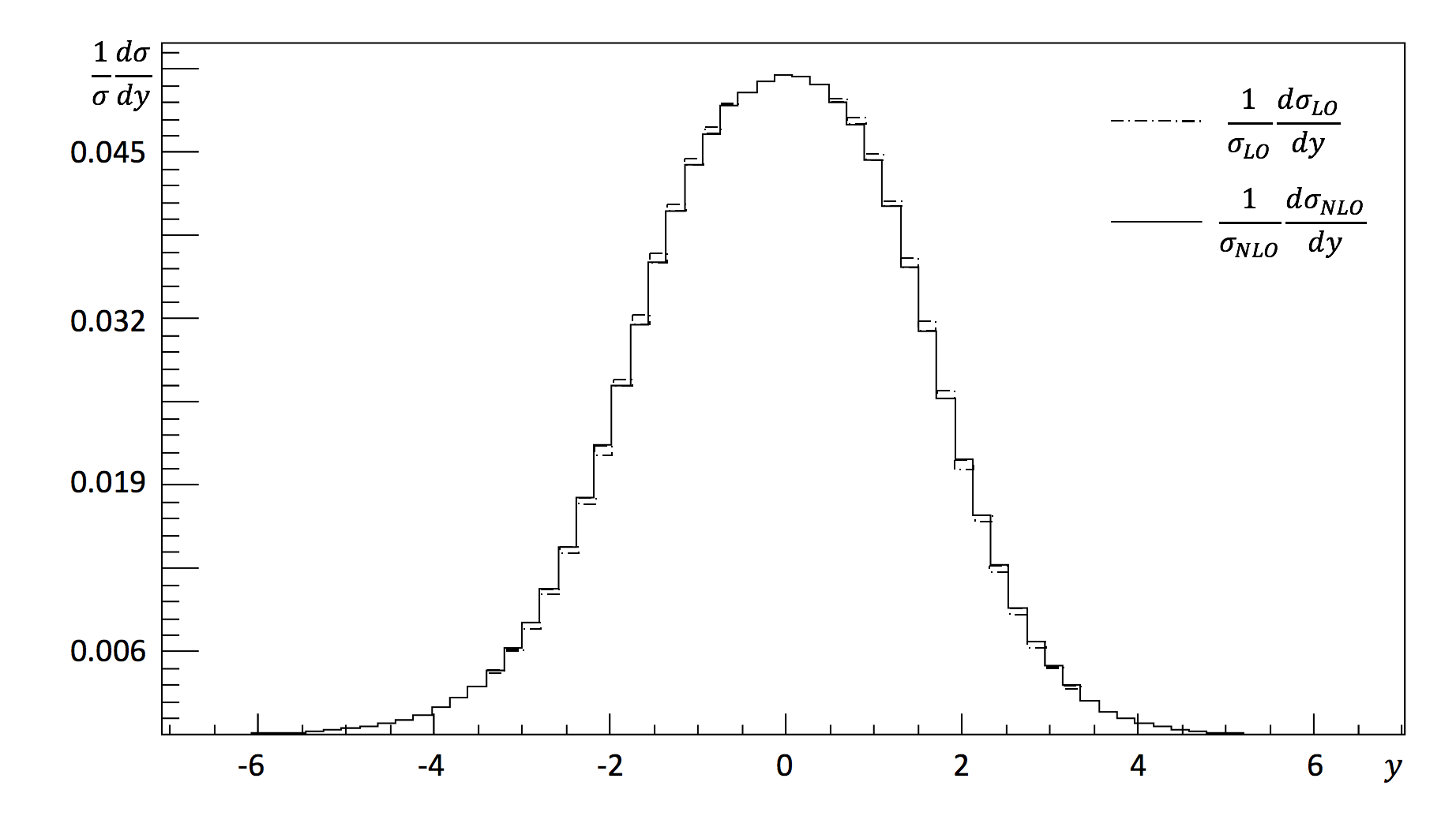
Figure 8: Differential cross-section for coloron pair production in terms of rapidity at LO and NLO accuracy, for $\sqrt{s}=14\,\,\mathrm{TeV}$, mass $M=1\,\,\mathrm{TeV}$, and $\mu=\mu_{\rm F}=M$.

5 Conclusions

The production of colored new physics particles at the LHC may be subject to sizeable QCD corrections. In this article, results for the NLO corrections to the pair production of color-octet vector bosons have been presented. Such new vector bosons appear, for example, in coloron models or models with extra space dimensions. There are characteristic versions of these models where the single production of color-octet vector bosons is forbidden by a parity symmetry, such as an exchange symmetry for coloron models and Kaluza-Klein parity for extra dimensional models. For concreteness, this paper focuses on a two-site coloron model, which is based on two copies of a non-linear sigma model for the gauge sector. In addition, the presence of the exchange symmetry requires the introduction of heavy partners to the SM quarks. This model can serve as a gauge-invariant low-energy effective description of the minimal universal extra dimension (mUED) model.

The renormalization of the two-site coloron model involves several peculiarities that do not occur for models with colored particles of spin less than one. For instance, the couplings of the SM gluon and the massive coloron are identical at tree-level, but they receive different counterterms at higher orders. In addition, the broken gauge symmetry of the massive vector boson requires the introduction of a counterterm for the symmetry-breaking vacuum expectation value. This may be surprising at first glance, given that the symmetry-breaking mechanism is not specified in the non-linear sigma model, but in fact this counterterm can be uniquely determined from the Goldstone self-energy.

The calculation of the NLO corrections presented in this paper is based on a largely automated computer implementation, using publicly available packages supplemented by in-house routines. For the combination of virtual loop corrections and real radiation contributions, the phase-space slicing method has been employed. Several checks of the results have been performed.

It is found that for the standard choice of the renormalization scale, $\mu=M$, where $M$ is the coloron mass, the NLO correction has a relatively modest impact on the coloron pair production cross-section. The total NLO cross-section is 11–14% smaller than the LO result for values of $M$ between 1 and 2 TeV. At the same time, the dependence of the cross-section on the renormalization scale is significantly reduced, by a factor of 2–3. By studying the rapidity distribution it is furthermore observed that the NLO contribution cannot be characterized by a simple global K-factor, but instead the K-factor is slightly smaller in the central rapidity region and slightly larger for large absolute values of rapidity.

Appendix A Feynman rules of the two-site coloron model

This appendix lists the tree-level Feynman rules of the two-site symmetric coloron model. The following notation is used:

$i,j,...$	color indices in the fundamental representation
$A,B,...$	color indices in the adjoint representation
$p_{X}$	incoming momentum of the particle with color index $X$
$\psi$	generic SM quark
$\Psi$	generic $\cal P$-odd quark
$Q$	SU(2)-doublet $\cal P$-odd quark
$U$	SU(2)-singlet $\cal P$-odd quark
$T,T^{\prime}$	$\cal P$-odd top partners, see eq. (17)
$\theta_{T}$	mixing angle defined in eq. (18)
$P_{L,R}=\frac{1}{2}(1\pm\gamma_{5})$
$\eta^{\mu\nu}$	metric tensor, $(\eta^{\mu\nu})=\text{diag}(1,-1,-1,-1)$
Line styles:
single solid	SM quark
double solid	$\cal P$-odd quark
spring	gluon
spring–solid	coloron
dashed	$\cal P$-odd Goldstone scalar
dotted	ghost

A.1 Feynman rules involving quarks except for the top quark

$$-ig_{\rm s}\gamma^{\mu}T^{A}_{ij}$$ (40)

$$-ig_{\rm s}\gamma^{\mu}T^{A}_{ij}$$ (41)

$$-ig_{\rm s}\gamma^{\mu}P_{L}T^{A}_{ij}$$ (42)

$$ig_{\rm s}\gamma^{\mu}P_{R}T^{A}_{ij}$$ (43)

$$-g_{\rm s}P_{R}T^{a}_{ij}$$ (44)

$$g_{\rm s}P_{L}T^{a}_{ij}$$ (45)

A.2 Vertices involving the top quark

$$-ig_{\rm s}\gamma^{\mu}\left[\sin{\theta_{T}}P_{R}+\cos{\theta_{T}}P_{L}\right]T^{a}_{ij}$$ (46)

$$ig_{\rm s}\gamma^{\mu}\left[\sin{\theta_{T}}P_{L}+\cos{\theta_{T}}P_{R}\right]T^{a}_{ij}$$ (47)

$$g_{\rm s}\left[\sin{\theta_{T}}P_{L}-\cos{\theta_{T}}P_{R}\right]T^{a}_{ij}$$ (48)

$$-g_{\rm s}\left[\sin{\theta_{T}}P_{R}-\cos{\theta_{T}}P_{L}\right]T^{a}_{ij}$$ (49)

A.3 Three-point boson vertices

$$g_{\rm s}\left[\left(p_{B}-p_{A}\right)^{\rho}\eta^{\mu\nu}+\left(p_{A}-p_{C}\right)^{\nu}\eta^{\mu\rho}+\left(p_{C}-p_{B}\right)^{\mu}\eta^{\nu\rho}\right]f^{ABC}$$

$$g_{\rm s}\left[\left(p_{B}-p_{A}\right)^{\rho}\eta^{\mu\nu}+\left(p_{A}-p_{C}\right)^{\nu}\eta^{\mu\rho}+\left(p_{C}-p_{B}\right)^{\mu}\eta^{\nu\rho}\right]f^{ABC}$$

$$-ig_{\rm s}M\eta^{\mu\nu}f^{ABC}$$ (52)

$$g_{\rm s}\left(p_{B}-p_{C}\right)^{\mu}f^{ABC}$$ (53)

A.4 Feynman rules involving ghosts

$$-g_{\rm s}p_{B}^{\mu}f^{ABC}$$ (54)

$$-g_{\rm s}p_{B}^{\mu}f^{ABC}$$ (55)

$$-g_{\rm s}p_{B}^{\mu}f^{ABC}$$ (56)

$$-ig_{\rm s}Mf^{ABC}$$ (57)

A.5 Four-point boson vertices

$$-ig_{\rm s}^{2}\bigl{[} \eta^{\mu\nu}\eta^{\rho\sigma}\bigl{(}f^{ACE}f^{BDE}-f^{ADE}f^{CBE}\bigr{)}$$

$$+ \eta^{\mu\rho}\eta^{\nu\sigma}\bigl{(}f^{ADE}f^{CBE}-f^{ABE}f^{DCE}\bigr{)}$$

$$+ \eta^{\mu\sigma}\eta^{\nu\rho}\bigl{(}f^{ABE}f^{DCE}-f^{ACE}f^{BDE}\bigr{)}\bigr{]}$$ (58)

$$-ig_{\rm s}^{2}\bigl{[} \eta^{\mu\nu}\eta^{\rho\sigma}\bigl{(}f^{ACE}f^{BDE}-f^{ADE}f^{CBE}\bigr{)}$$

$$+ \eta^{\mu\rho}\eta^{\nu\sigma}\bigl{(}f^{ADE}f^{CBE}-f^{ABE}f^{DCE}\bigr{)}$$

$$+ \eta^{\mu\sigma}\eta^{\nu\rho}\bigl{(}f^{ABE}f^{DCE}-f^{ACE}f^{BDE}\bigr{)}\bigr{]}$$ (59)

$$-ig_{\rm s}^{2}\bigl{[} \eta^{\mu\nu}\eta^{\rho\sigma}\bigl{(}f^{ACE}f^{BDE}-f^{ADE}f^{CBE}\bigr{)}$$

$$+ \eta^{\mu\rho}\eta^{\nu\sigma}\bigl{(}f^{ADE}f^{CBE}-f^{ABE}f^{DCE}\bigr{)}$$

$$+ \eta^{\mu\sigma}\eta^{\nu\rho}\bigl{(}f^{ABE}f^{DCE}-f^{ACE}f^{BDE}\bigr{)}\bigr{]}$$ (60)

$$ig_{\rm s}^{2}\eta^{\mu\nu}\left(f^{ACE}f^{BDE}+f^{BCE}f^{ADE}\right)$$ (61)

$$ig_{\rm s}^{2}\eta^{\mu\nu}\left(f^{ACE}f^{BDE}+f^{BCE}f^{ADE}\right)$$ (62)

Note that the Feynman rules in this appendix agree with those for KK-level–1 gluons and quarks in mUED, with the exception of (60), which has an additional factor $\frac{3}{2}$ in mUED.

References

- [1] T. Appelquist, H. C. Cheng and B. A. Dobrescu, Phys. Rev. D 64, 035002 (2001) [hep-ph/0012100].
- [2] D. Hooper and S. Profumo, Phys. Rept. 453, 29 (2007) [hep-ph/0701197].
- [3] C. T. Hill, Phys. Lett. B 266, 419 (1991).
- [4] C. T. Hill and S. J. Parke, Phys. Rev. D 49, 4454 (1994) [hep-ph/9312324]; R. S. Chivukula, A. G. Cohen and E. H. Simmons, Phys. Lett. B 380, 92 (1996) [hep-ph/9603311].
- [5] L. Randall, Nucl. Phys. B 403, 122 (1993) [hep-ph/9210231]; G. Burdman and N. J. Evans, Phys. Rev. D 59, 115005 (1999) [hep-ph/9811357].
- [6] E. H. Simmons, Phys. Rev. D 55, 1678 (1997) [hep-ph/9608269]; A. Atre, R. S. Chivukula, P. Ittisamai, E. H. Simmons and J. H. Yu, Phys. Rev. D 86, 054003 (2012) [arXiv:1206.1661 [hep-ph]]; R. Sekhar Chivukula, P. Ittisamai and E. H. Simmons, Phys. Rev. D 91, no. 5, 055021 (2015) [arXiv:1406.2003 [hep-ph]].
- [7] G. Aad et al. [ATLAS Collaboration], JHEP 1508, 148 (2015) [arXiv:1505.07018 [hep-ex]]; G. Aad et al. [ATLAS Collaboration], Phys. Lett. B 754, 302 (2016) [arXiv:1512.01530 [hep-ex]]; M. Aaboud et al. [ATLAS Collaboration], Phys. Lett. B 759, 229 (2016) [arXiv:1603.08791 [hep-ex]].
- [8] V. Khachatryan et al. [CMS Collaboration], Phys. Rev. D 93, no. 1, 012001 (2016) [arXiv:1506.03062 [hep-ex]]; A. M. Sirunyan et al. [CMS Collaboration], arXiv:1611.03568 [hep-ex].
- [9] T. G. Rizzo, Phys. Rev. D 64, 095010 (2001) [hep-ph/0106336]; C. Macesanu, C. D. McMullen and S. Nandi, Phys. Rev. D 66, 015009 (2002) [hep-ph/0201300]; H. C. Cheng, K. T. Matchev and M. Schmaltz, Phys. Rev. D 66, 056006 (2002) [hep-ph/0205314]; A. Datta, K. Kong and K. T. Matchev, Phys. Rev. D 72, 096006 (2005), Erratum: Phys. Rev. D 72, 119901 (2005) [hep-ph/0509246]; J. M. Smillie and B. R. Webber, JHEP 0510, 069 (2005) [hep-ph/0507170]; J. A. R. Cembranos, J. L. Feng and L. E. Strigari, Phys. Rev. D 75, 036004 (2007) [hep-ph/0612157].
- [10] W. Beenakker, R. Höpker, M. Spira and P. M. Zerwas, Nucl. Phys. B 492, 51 (1997) [hep-ph/9610490].
- [11] W. Beenakker, M. Krämer, T. Plehn, M. Spira and P. M. Zerwas, Nucl. Phys. B 515, 3 (1998) [hep-ph/9710451].
- [12] W. Beenakker, C. Borschensky, M. Krämer, A. Kulesza, E. Laenen, V. Theeuwes and S. Thewes, JHEP 1412, 023 (2014) [arXiv:1404.3134 [hep-ph]]; W. Beenakker, C. Borschensky, R. Heger, M. Krämer, A. Kulesza and E. Laenen, JHEP 1605, 153 (2016) [arXiv:1601.02954 [hep-ph]].
- [13] M. Krämer, T. Plehn, M. Spira and P. M. Zerwas, Phys. Rev. Lett. 79, 341 (1997) [hep-ph/9704322].
- [14] M. Cacciari, M. Czakon, M. Mangano, A. Mitov and P. Nason, Phys. Lett. B 710, 612 (2012) [arXiv:1111.5869 [hep-ph]].
- [15] D. Gonçalves-Netto, D. López-Val, K. Mawatari, T. Plehn and I. Wigmore, Phys. Rev. D 85, 114024 (2012) [arXiv:1203.6358 [hep-ph]].
- [16] R. S. Chivukula, A. Farzinnia, E. H. Simmons and R. Foadi, Phys. Rev. D 85, 054005 (2012) [arXiv:1111.7261 [hep-ph]].
- [17] R. S. Chivukula, A. Farzinnia, J. Ren and E. H. Simmons, Phys. Rev. D 87, no. 9, 094011 (2013) [arXiv:1303.1120 [hep-ph]].
- [18] S. R. Coleman, J. Wess and B. Zumino, Phys. Rev. 177, 2239 (1969); C. G. Callan, S. R. Coleman, J. Wess and B. Zumino, Phys. Rev. 177, 2247 (1969).
- [19] A. Datta, K. Kong and K. Matchev, “Minimal Universal Extra Dimensions in CalcHEP/CompHEP,” http://home.fnal.gov/~kckong/mued/mued.pdf.
- [20] A. Mück, A. Pilaftsis and R. Rückl, Phys. Rev. D 65, 085037 (2002) [hep-ph/0110391].
- [21] H. Georgi, A. K. Grant and G. Hailu, Phys. Lett. B 506, 207 (2001) [hep-ph/0012379]; H. C. Cheng, K. T. Matchev and M. Schmaltz, Phys. Rev. D 66, 036005 (2002) [hep-ph/0204342].
- [22] V. Ilisie, “Concepts in Quantum Field Theory: A Practitioner’s Toolkit,” Springer, Switzerland (2016), chapter 9.3.
- [23] B. W. Harris and J. F. Owens, Phys. Rev. D 65, 094032 (2002) [hep-ph/0102128].
- [24] W. Beenakker, H. Kuijf, W. L. van Neerven and J. Smith, Phys. Rev. D 40, 54 (1989).
- [25] T. Hahn, Comput. Phys. Commun. 140, 418 (2001) [hep-ph/0012260].
- [26] V. Shtabovenko, R. Mertig and F. Orellana, Comput. Phys. Commun. 207, 432 (2016) [arXiv:1601.01167 [hep-ph]].
- [27] G. Passarino and M. J. G. Veltman, Nucl. Phys. B 160, 151 (1979).
- [28] T. Hahn, PoS ACAT 2010, 078 (2010) [arXiv:1006.2231 [hep-ph]].
- [29] R. K. Ellis and G. Zanderighi, JHEP 0802, 002 (2008) [arXiv:0712.1851 [hep-ph]].
- [30] A. Buckley, J. Ferrando, S. Lloyd, K. Nordström, B. Page, M. Rüfenacht, M. Schönherr and G. Watt, Eur. Phys. J. C 75, 132 (2015) [arXiv:1412.7420 [hep-ph]].
- [31] D. Stump, J. Huston, J. Pumplin, W. K. Tung, H. L. Lai, S. Kuhlmann and J. F. Owens, JHEP 0310, 046 (2003) [hep-ph/0303013].
-
[32]
M. R. Whalley, D. Bourilkov and R. C. Group,
hep-ph/0508110;
http://lhapdf.hepforge.org. - [33] G. Aad et al. [ATLAS Collaboration], JHEP 1504, 116 (2015) [arXiv:1501.03555 [hep-ex]]; N. Deutschmann, T. Flacke and J. S. Kim, Phys. Lett. B 771, 515 (2017) [arXiv:1702.00410 [hep-ph]]; J. Beuria, A. Datta, D. Debnath and K. T. Matchev, arXiv:1702.00413 [hep-ph].