Towards simulating and quantifying the light-cone EoR 21-cm signal

Abstract

The light-cone (LC) effect causes the Epoch of Reionization (EoR) 21-cm signal $T_{\rm b}(\hat{\bm{n}},\nu)$ to evolve significantly along the line of sight (LoS) direction $\nu$. In the first part of this paper we present a method to properly incorporate the LC effect in simulations of the EoR 21-cm signal that include peculiar velocities. Subsequently, we discuss how to quantify the second order statistics of the EoR 21-cm signal in the presence of the LC effect. We demonstrate that the 3D power spectrum $P({\bm{k}})$ fails to quantify the entire information because it assumes the signal to be ergodic and periodic, whereas the LC effect breaks these conditions along the LoS. Considering a LC simulation centered at redshift $8$ where the mean neutral fraction drops from $0.65$ to $0.35$ across the box, we find that $P({\bm{k}})$ misses out $\sim 40\%$ of the information at the two ends of the $17.41\,{\rm MHz}$ simulation bandwidth. The multi-frequency angular power spectrum (MAPS) ${\mathcal{C}}_{\ell}(\nu_{1},\nu_{2})$ quantifies the statistical properties of $T_{\rm b}(\hat{\bm{n}},\nu)$ without assuming the signal to be ergodic and periodic along the LoS. We expect this to quantify the entire statistical information of the EoR 21-cm signal. We apply MAPS to our LC simulation and present preliminary results for the EoR 21-cm signal.

1 Introduction

Observation of the redshifted 21-cm signal from neutral hydrogen (H i), one of the most promising tools to probe the epoch of reionization (EoR), is currently a frontier of modern astrophysics and cosmology. There is a tremendous effort, all over the globe, to detect the EoR 21-cm signal either statistically or around bright individual objects using ongoing and upcoming radio interferometric experiments e.g. GMRT (Ghosh et al., 2012; Paciga et al., 2013), LOFAR (van Haarlem et al., 2013; Yatawatta et al., 2013), MWA (Bowman et al., 2013; Tingay et al., 2013; Dillon et al., 2014), PAPER (Parsons et al., 2014; Ali et al., 2015; Jacobs et al., 2015), SKA (Mellema et al., 2013; Koopmans et al., 2015) and HERA (Furlanetto et al., 2009).

One of the major advantages of the redshifted H i 21-cm signal is that it allows one to map the large scale structure of the universe in 3D with the third axis being the cosmic time (or redshift). However, the mean as well as the statistical properties of H i 21-cm signal change with redshift. This effect, known as the ‘light-cone’ (LC) effect, has a significant impact on the observable quantities such as on H i 21-cm brightness temperature maps, power spectrum, etc. It is thus important to correctly include this effect to predict the signal and to also interpret the observations.

The issue was first considered in Barkana & Loeb (2006) who analytically modelled the anisotropies in the two-point correlation function arising due to the LC effect. A similar approach was later followed in Zawada et al. (2014) which used large scale numerical simulations and studied, in more details, the LC anisotropies in the two point correlation function. Datta et al. (2012) first investigated the impact of the LC effect on the spherically averaged H i power spectrum which is one of the primary observables for all the ongoing and upcoming radio interferometric telescopes mentioned earlier. They find that the effect mainly ‘averages out’ in the spherically averaged power spectrum and they report a change of up to $\sim 50\%$ at the large scales corresponding to a frequency bandwidth of $\sim 8\,{\rm MHz}$. Subsequently, ${\rm Gpc}$ size simulations have been used to investigate various other issues such as quantifying the LC induced anisotropies in the power spectrum and determining the optimal bandwidth for analyzing the observed signal in order to avoid complexities arising from the LC effect (La Plante et al., 2014; Datta et al., 2014). In a recent work Ghara et al. 2015 have considered the H i 21-cm signal from the cosmic dawn which includes fluctuations in the spin temperature. They find that the LC effect has a dramatic signature on the cosmic dawn H i power spectrum.

The redshift space distortion due to peculiar velocities is an important effect that modifies the redshifted 21-cm signal (Bharadwaj & Ali, 2004) along the line of sight (LoS). While there has been considerable work on including this effect in simulations of the EoR 21-cm signal (Mao et al., 2012; Majumdar et al., 2013; Jensen et al., 2013), the issue of how to properly include the LC effect in the presence of peculiar velocities has not been addressed earlier.

The issue of how to analyze the statistics of the EoR 21-cm signal in the presence of the LC effect is also important. Note that the signal in the different Fourier modes is uncorrelated only for a statistically homogeneous or ergodic signal, and in this case the second order statistics is completely quantified by the 3D power spectrum $P({\bm{k}})$. However, the LC effect breaks statistical homogeneity and makes the signal non-ergodic along the LoS. In this case the signal in the different Fourier modes along the LoS is correlated. This implies that $P({\bm{k}})$ does not retain the entire information of the 21-cm signal. Trott (2016) has argued that the spherically averaged H i 21-cm power spectrum gives a biased estimate of the EoR 21-cm signal and has proposed the use of the wavelet transform to obtain an improved estimate in comparison to the standard Fourier transform.

In this work we address two issues. First, how to properly incorporate the LC effect in simulations of the EoR 21-cm signal in the presence of peculiar velocities. Second, how to properly quantify the statistical properties of the EoR 21-cm signal. To this end we consider the multi-frequency angular power spectrum (MAPS, Datta et al. 2007) which doesn’t assume the signal to be ergodic along the LoS and retains the full information of the 21-cm signal.

Throughout this paper, we have used the Planck+WP best fit values of cosmological parameters $\Omega_{\rm m0}=0.3183$, $\Omega_{\rm\Lambda 0}=0.6817$, $\Omega_{\rm b0}h^{2}=0.022032$, $h=0.6704$, $\sigma_{8}=0.8347$, and $n_{\rm s}=0.9619$ (Planck Collaboration et al., 2014).

2 Simulating the light-cone effect

The redshifted EoR H i 21-cm signal is the quantity of interest here. The Hydrogen distribution evolves dramatically across the EoR. Starting from the early stages of EoR when the mean mass weighted Hydrogen neutral fraction $\bar{x}_{\rm\text{H\,{i}}}$ is close to $1$, the Hydrogen distribution evolves rapidly to a situation where it is nearly completely ionized with $\bar{x}_{\rm\text{H\,{i}}}\sim 0$ at the end of reionization. The issue here is ‘How to incorporate the light-cone (LC) effect in simulations of the EoR 21-cm signal?’.

The light-cone (LC) effect refers to the fact that our view of the Universe is restricted to the backward light cone which imposes the relation

$$r=c(\eta_{0}-\eta)\,,$$ (1)

between the comoving distance $r$ as measured from our position and the conformal time $\eta$, the suffix ‘$0$’ here refers to the present epoch. We consider a simulation that span the comoving distance range $r_{\rm n}$ (nearest) to $r_{\rm f}$ (farthest). The LC effect implies that our view at $r_{\rm f}$ is restricted to an early epoch $\eta_{\rm f}$ (eq. 1) when the universe is largely neutral whereas at $r_{\rm n}$ it is restricted to a later epoch $\eta_{\rm n}$ when the universe is nearly completely reionized. At each distance in the range $r_{\rm n}\leq r\leq r_{\rm f}$, we view a different stage of the cosmological evolution $\eta_{\rm f}\leq\eta\leq\eta_{\rm n}$ and consequently $\bar{x}_{\rm\text{H\,{i}}}$ evolves along the radial direction of the simulation volume. It is particularly important to account for this evolution when simulating the EoR 21-cm signal.

For our purpose we have simulated snapshots of the H i distribution (so called coeval cubes) at 25 different epochs $\eta_{\rm i}$ that span the relevant range $\eta_{\rm f}\leq\eta_{\rm i}\leq\eta_{\rm n}$ at non-uniform intervals $\Delta\eta_{\rm i}$ which were chosen so that $\bar{x}_{\rm\text{H\,{i}}}$ varies by approximately an equal amount in each interval. The H i distribution in our simulations is represented by particles whose H i masses vary with position depending on the local Hydrogen neutral fraction. Each snapshot provides the positions, peculiar velocities and H i masses of these particles. Each epoch $\eta_{\rm i}$ corresponds to a different radial distance $r_{\rm i}$ in the simulation volume (eq. 1). To construct the LC simulation we have sliced the simulation volume at these $r_{\rm i}$, and for each slice we have filled the region $r_{\rm i}$ to $r_{\rm i+1}$ with the H i particles from the corresponding region in the snapshot at the epoch $\eta_{\rm i}$ (Fig. 1).

\psfrag{etai-1}[c][c][1][0]{$\eta_{\rm i-1}$~{}~{}}\psfrag{etai}[c][c][1][0]{$\eta_{\rm i}$~{}~{}~{}}\psfrag{Coeval}[c][c][1][0]{\large Coeval\,}\psfrag{ri-1 ri}[c][c][1][0]{~{}$r_{\rm i-1}\,r_{\rm i}$}\psfrag{ri ri+1}[c][c][1][0]{~{}~{}$r_{\rm i}\,r_{\rm i+1}$}\psfrag{Light-cone}[c][c][1][0]{\large Light-cone}\psfrag{etai-1 eti}[c][c][1][0]{$\eta_{\rm i-1}\,\eta_{\rm i}$~{}~{}}\psfrag{ri-1 ri ri+1}[c][c][1][0]{~{}$r_{\rm i-1}\,r_{\rm i}\,r_{\rm i+1}$}\includegraphics[width=177.78578pt]{figs/lightcone_new.eps}

Figure 1: This schematically shows how we sliced the coeval simulations and stitched the slices to form the LC simulation. The top panels represent our coeval simulations (at $\eta_{\rm i-1}$ and $\eta_{\rm i}$ respectively) and the bottom panel represents the LC simulation. Note that the spherical coordinate system has origin at a distant observer located on the left.

Observations will yield brightness temperature fluctuations $\delta{T_{\rm b}}(\hat{\bm{n}},\nu)$ which are measured as a function of the observing frequency $\nu$ and direction $\hat{\bm{n}}$, here $\hat{\bm{n}}$ is the unit vector in the direction of observation. For the 21-cm signal originating from the point $\hat{\bm{n}}\,r$, the cosmological expansion and the radial component of the H i peculiar velocity $\hat{\bm{n}}\cdot\bm{v}(\hat{\bm{n}}r,\eta)$ together determine the frequency $\nu$ at which the signal observed, and we have

$$\nu=a(\eta)[1-\hat{\bm{n}}\cdot\bm{v}(\hat{\bm{n}}r,\eta)/c]\times\nu_{\rm e}\,,$$ (2)

where $\nu_{\rm e}=1,420\,{\rm MHz}$. For a fixed direction $\hat{\bm{n}}$, we can view eqs. (1) and (2) together as a map $r\rightarrow\nu$ from comoving distance $r$ to frequency $\nu$. Considering the different shells within the LC simulation (Fig. 1), we can assign a frequency $\nu_{\rm i}=a(\eta_{\rm i})\nu_{\rm e}$ to the boundary $r_{\rm i}$ of each of these shells. We now consider a simulation particle labelled $m$ located at the position ${\bm{r}}_{\rm m}=r_{\rm m}\hat{\bm{n}}_{\rm m}$ within the $i$-th shell $(r_{\rm i}\leq r_{\rm m}<r_{\rm i+1})$. We use eq. (2) to assign the frequency

$$\nu_{\rm m}=\nu_{\rm i}\left[1-\frac{a_{\rm i}H_{\rm i}(r_{\rm m}-r_{\rm i})+\hat{\bm{n}}_{\rm m}\cdot\bm{v}_{\rm m}}{c}\right]$$ (3)

to the redshifted 21-cm signal from the H i associated with this particle. Here scale factor $a_{\rm i}\equiv a(\eta_{\rm i})$ and Hubble parameter $H_{\rm i}\equiv H(\eta_{\rm i})$ respectively. We use eq. (3) to map the H i distribution within the LC simulation from ${\bm{r}}=r\hat{\bm{n}}$ to $\nu$ and $\hat{\bm{n}}$ which are the variables relevant for observations of the 21-cm brightness temperature.

Assuming that the spin temperature is much greater than the background CMB temperature i.e. $T_{\rm s}\gg T_{\gamma}$, the H i 21-cm brightness temperature (eq. 4 and A5 of Bharadwaj & Ali 2005) can be expressed as

$$T_{\rm b}(\hat{\bm{n}},\nu)=\bar{T}_{0}\,\frac{\rho_{\text{H\,{i}}}}{\bar{\rho}_{\rm H}}\,\left(\frac{H_{0}\nu_{\rm e}}{c}\right)\,\bigg{|}\frac{\partial r}{\partial\nu}\bigg{|}\,,$$ (4)

where

$$\bar{T}_{0}=4.0{\rm mK}\,\left(\frac{\Omega_{\rm b}h^{2}}{0.02}\right)\left(\frac{0.7}{h}\right)\,,$$ (5)

${\rho_{\text{H\,{i}}}}/{\bar{\rho}_{\rm H}}$ is the ratio of the neutral hydrogen to the mean hydrogen density, and here it is convenient to use the respective comoving densities. Eqs. (1) and (2) together imply a map from $r$ to $\nu$, and ${\partial r}/{\partial\nu}$ refers to the derivative of this map.

We note that the comoving H i density can be obtained by assigning the H i mass in the particles to an uniform rectangular grid in comoving space

$$\rho_{\text{H\,{i}}}=(\Delta r)^{-3}\sum_{m}[M_{\text{H\,{i}}}]_{\rm m}$$ (6)

where $(\Delta r)^{3}$ is the volume of each grid cell. Here we use an uniform grid in solid angle $(\Delta\Omega)$ and frequency $(\Delta\nu)$ to define a modified density $\rho^{\prime}_{\text{H\,{i}}}$ calculated using

$$\rho^{\prime}_{\text{H\,{i}}}=(\Delta\Omega\,\Delta\nu)^{-1}\left(\frac{H_{0}\nu_{\rm e}}{c}\right)\sum_{m}\frac{[M_{\text{H\,{i}}}]_{\rm m}}{r_{\rm n}^{2}}\,.$$ (7)

Comparing eqs. (6) and (7) we see that we can write the brightness temperature (eq. 4) in terms of $\rho^{\prime}_{\text{H\,{i}}}$ as

$$T_{\rm b}(\hat{\bm{n}},\nu)=\bar{T}_{0}\,\frac{\rho^{\prime}_{\text{H\,{i}}}}{\bar{\rho}_{\rm H}}\,.$$ (8)

We have used eq. (8) to calculate the redshifted 21-cm brightness temperature distribution ${T_{\rm b}}(\hat{\bm{n}}r)$ from the H i distribution in the LC simulation.

2.1 Generating the coeval cubes

We have simulated the coeval ionization cubes with a co-moving length $L=300.16~{}{\rm Mpc}$ on each side using semi-numerical simulations which involve three main steps. First, we use a particle mesh $N$-body code to generate the dark matter distribution. We have run simulations with $4288^{3}$ grids of spacing $0.07\,{\rm Mpc}$ and a mass resolution of $1.09\times 10^{8}\,M_{\sun}$. In the next step, we use the Friends-of-Friends (FoF) algorithm to identify collapsed halos in the dark matter distribution. We have used a fixed linking length of $0.2$ times the mean inter-particle distance and also set the criterion that a halo should have at least $10$ dark matter particles. The third and final step generates the ionization map using the parameters $\{N_{\rm ion},\,M_{\rm halo,min},\,R_{\rm mfp}\}=\{23.21,\,1.09\times 10^{9}~{}M_{\sun},\,20~{}{\rm Mpc}\}$ (same as Mondal et al. 2017, 2016; Mondal et al. 2015) based on the excursion set formalism of Furlanetto et al. (2004). Our semi-numerical simulations closely follow the homogeneous recombination scheme of Choudhury et al. (2009). The H i distribution in our simulations is represented by particles whose H i masses were calculated from the neutral Hydrogen fraction $x_{\rm\text{H\,{i}}}$ interpolated from its eight nearest neighbouring grid points. Each coeval cube provides the positions, peculiar velocities and H i masses of these particles.

\psfrag{xh1}[c][c][1][0]{\large$\bar{x}_{\rm\text{H\,{i}}}$}\psfrag{z}[c][c][1][0]{\large Redshift}\psfrag{r}[c][c][1][0]{\large$r-r_{\rm c}~{}$Mpc}\psfrag{10}[c][c][1][0]{\large$10$}\includegraphics[width=195.12767pt]{figs/z_xh1.eps}

Figure 2: This shows the reionization history as a function of co-moving distance ($r-r_{\rm c}$) that we have obtained from our semi-numerical simulations. We have generated the coeval cubes at different $r_{\rm i}$ that span the shaded region. The redshift values corresponding to different co-moving distances are shown on the top $x$-axis.

We have used the semi-numerical simulations to generate the reionization history, which is shown in Fig. 2. We have generated the coeval cubes at different co-moving distance $r_{\rm i}$ that span the range $r_{\rm n}=9001.45~{}{\rm Mpc}$ (nearest) to $r_{\rm f}=9301.61~{}{\rm Mpc}$ (farthest), which correspond to the redshifts $7.51$ and $8.53$ respectively. The change in the mass-averaged H i fraction $\bar{x}_{\rm\text{H\,{i}}}$ over the aforesaid $r$ range, according to our reionization history (Fig. 2), is $\Delta\bar{x}_{\rm\text{H\,{i}}}\approx 0.65-0.35=0.30$. We have chosen $25$ different $r_{\rm i}$ so that $\bar{x}_{\rm\text{H\,{i}}}$ varies by approximately an equal amount in each interval. Using these coeval H i cubes, we have generated our light-cone (LC) box following the formalism presented in Section 2. The LC box is centered at redshift $8$ which correspond to the co-moving distance $r_{\rm c}=9151.53~{}{\rm Mpc}$, frequency $\nu_{\rm c}=157.78\,{\rm MHz}$ and $\bar{x}_{\rm\text{H\,{i}}}\approx 0.51$.

2.2 Flat-sky approximation

The observed sky is spherical and the slices simulated at fixed values of $r_{\rm i}$ are, in general, curved as shown in Fig. 1. However, the angular extent $\theta_{\rm max}=L/(2r_{\rm f})$ of our simulation box is $\approx 1^{\circ}$ for which it is adequate to adopt the flat-sky approximation whereby the simulation slices are flat as shown in Fig. 3. We use a Cartesian coordinate system with the origin located at the distant observer, the $z$ axis is aligned along the LoS through the centre of the box, and the $x$ and $y$ axes are in the plane of the sky – perpendicular to the $z$-axis. Under the flat-sky approximation, the unit vector $\hat{\bm{n}}$ along any arbitrary direction can be decomposed as $\hat{\bm{n}}=\hat{\bm{k}}+{\bm{\theta}}$ where $\hat{\bm{k}}$ is the unit vector along the $z$-axis and ${\bm{\theta}}$ is a 2D vector in the plane of the sky. The curvature of the sky introduces terms of order $\theta^{2}$ and higher which we have ignored here in the flat-sky approximation. We have, however, retained terms of order $\theta$ ensuring that the resulting errors are of order $<1\%$. In particular we use the approximations $r=\sqrt{z^{2}+x^{2}+y^{2}}\approx z$, ${\bm{\theta}}\approx[(x/z){\hat{\bm{i}}}+(y/z){\hat{\bm{j}}}]$ and $\hat{\bm{n}}_{\rm m}\cdot\bm{v}_{\rm m}\approx[v_{\rm z}]_{\rm m}+(x/z)\,[v_{\rm x}]_{\rm m}+(y/z)\,[v_{\rm y}]_{\rm m}$.

\psfrag{nm}[c][c][1][0]{$\hat{\bm{n}}_{\rm m}$}\psfrag{rm}[c][c][1][0]{$r_{\rm m}$}\psfrag{theta}[c][c][1][0]{~{}$\theta_{\rm m}$}\psfrag{z}[c][c][1][0]{$z$}\psfrag{o}[c][c][1][0]{~{}~{}o}\psfrag{ri ri+1}[c][c][1][0]{~{}~{}~{}~{}$r_{\rm i}\,\,~{}~{}~{}~{}r_{\rm i+1}$}\includegraphics[width=195.12767pt]{figs/flat_sky.eps}

Figure 3: This shows the $m$-th particle within $i$-th LC slice at $r_{\rm m}$ in the flat-sky approximation.

We use eq. (3) to map the positions of the H i particles to frequency space. The final LC simulation extends from $\nu_{\rm f}$ to $\nu_{\rm n}$ in frequency, and we note that the inclusion of peculiar velocities causes some of the particles to have frequency values beyond the box boundaries. This causes a depletion in the particle density near the box boundaries. We have estimated the frequency interval that is affected by this particle depletion, and we have excluded slices of this size from both the nearest and farthest sides of the LC box. Finally, we have interpolated the H i distribution from the particles to a 3D rectangular grid in $({\bm{\theta}},\,\nu)$. The bottom panel of Fig. 4 shows a section through the simulated 3D LC 21-cm brightness temperature map. The smaller frequencies on the right side of the LC simulation correspond to the earlier stages of the evolution as compared to the larger frequencies shown on the left side. For comparison, the top panel of Fig. 4 shows the same section through a coeval simulation at the central redshift $8$. The different frequencies in the coeval simulation all correspond to the same stage of the evolution. We see that it is possible to identify the same ionized regions in both the LC and coeval simulations. We see that at the right side (early stage) the ionized regions appear smaller in the LC simulation as compared to the coeval case, whereas the ionized regions appear larger in the LC simulation at the left side (later stage). The fact that each frequency corresponds to a different stage of the evolution is clearly evident if we compare the two panels of Fig. 4. We note that the brightness temperature fluctuations $\delta{T_{\rm b}}({\bm{\theta}},\nu)=T_{\rm b}({\bm{\theta}},\nu)-\bar{T}_{\rm b}(\nu)$ in the coeval simulations are, by construction, statistically homogeneous along the LoS direction $\nu$. The cosmological evolution seen in the LC simulation, however, breaks the statistical homogeneity along the LoS direction $\nu$. The fluctuations $\delta{T_{\rm b}}({\bm{\theta}},\nu)$ continue to be statistically homogeneous along ${\bm{\theta}}$ in both the coeval and LC simulations.

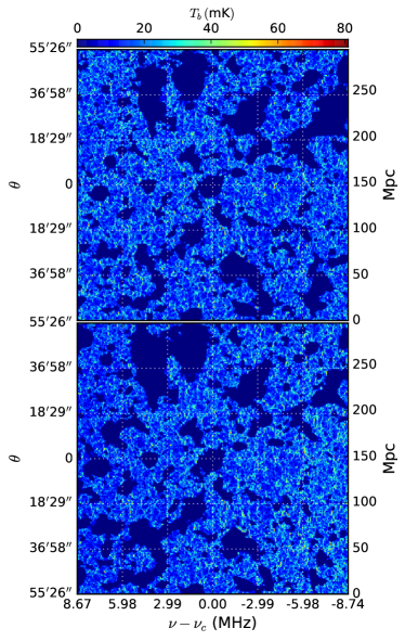
Figure 4: This shows ${T_{\rm b}}({\bm{\theta}},\nu)$ on a section through the 3D 21-cm brightness temperature maps for the LC (bottom) and coeval (top) simulations. The right vertical axis and the overlaid grid shows the corresponding comoving coordinates calculated using eq. (9).

3 Statistical analysis

The issue here is “How to quantify the statistics of $\delta{T_{\rm b}}({\bm{\theta}},\,\nu)$?”. We consider two statistical quantities namely the spherically averaged three dimensional (3D) power spectrum and the multi-frequency angular power spectrum (MAPS) which are discussed in the two subsequent sub-sections.

3.1 The power spectrum

Several authors (see Section 1) have used the 3D power spectrum $P({\bm{k}})$ to quantify the simulated EoR 21-cm signal in the presence of the LC effect. The first step here is to map the EoR 21-cm brightness temperature fluctuations to spatial comoving coordinates $\delta T_{\rm b}({\bm{\theta}},\nu)\rightarrow\delta T_{\rm b}(x,y,z)$ within the simulation volume $V$. The fact that $r$ varies with $\nu$ along the LoS and the two have a non-linear relation results in a spatial grid of non-uniform spacing which poses a problem for evaluating the Fourier transform needed to compute $P({\bm{k}})$. We have avoided this complication by using

$$(x,\,y,\,z)=(r_{\rm c}\,\theta_{\rm x},\,r_{\rm c}\,\theta_{\rm y},\,z_{\rm c}+r^{\prime}_{\rm c}\,(\nu-\nu_{\rm c})\,)$$ (9)

where $r_{\rm c}$ and $r^{\prime}_{\rm c}=\frac{d\,r}{d\,\nu}\big{|}_{r_{\rm c}}$ are both evaluated at the central redshift of $8$. This approximation results in a rectangular spatial grid of uniform spacing where we directly use FFT to estimate $\tilde{T}_{\rm b}({\bm{k}})$ which is the 3D Fourier transform of $\delta T_{\rm b}(x,y,z)$. This approximation introduces an error which is less than $\sim 2\%$ in grid positions.

The 3D H i 21-cm power spectrum can be calculated using

$$P({\bm{k}})=V^{-1}\big{\langle}\tilde{T}_{\rm b}({\bm{k}})\,\tilde{T}_{\rm b}(-{\bm{k}})\big{\rangle}\,.$$ (10)

Fig. 5 shows the dimensionless spherically averaged H i 21-cm power spectra $\Delta^{2}_{\rm b}(k)=k^{3}P(k)/2\pi^{2}$ as a function of $k$ for the LC and coeval simulations, both centred at redshift $8$. We see that the LC effect introduces a very significant enhancement at large scales and the two power spectra differ by factors of $\sim 4$ and $2$ at $k\sim 0.03\,{\rm Mpc}^{-1}$ and $0.05\,{\rm Mpc}^{-1}$ respectively. We note that these large scale modes are affected by the sample variance due to the finite size of simulation cubes used and actual value might change to some extent. Although the simulation methodology and the parameters used here are quite different, this result is consistent and qualitatively similar to those obtained earlier (Datta et al., 2012; La Plante et al., 2014; Datta et al., 2014).

\psfrag{pk}[c][c][1][0]{\large${\Delta^{2}_{\rm b}}\,\,{\rm mK^{2}}$}\psfrag{diff}[c][c][1][0]{${\delta\Delta^{2}_{\rm b}}/\Delta^{2}_{\rm b}$}\psfrag{k}[c][c][1][0]{\large$k\,~{}{\rm Mpc}^{-1}$}\psfrag{RS}[c][c][1][0]{\large Coeval~{}~{}~{}~{}}\psfrag{LC+RS}[c][c][1][0]{\large~{}~{}~{}~{}~{}LC}\includegraphics[width=195.12767pt,angle={0}]{figs/pk.eps}

Figure 5: This (top panel) shows the dimensionless spherically averaged H i 21-cm power spectrum $\Delta^{2}_{\rm b}(k)$. The bottom panel shows the relative difference ${\delta\Delta^{2}_{\rm b}}/\Delta^{2}_{\rm b}=\frac{[\Delta^{2}_{\rm b}]_{\rm LC}-[\Delta^{2}_{\rm b}]_{\rm Coeval}}{[\Delta^{2}_{\rm b}]_{\rm Coeval}}$.

It is important to note that the EoR 21-cm signal $\delta T_{\rm b}({\bm{\theta}},\nu)$ evolves significantly along the LoS direction $\nu$ due to the LC effect (Fig. 4). While the 3D Fourier modes and 3D power spectrum $P({\bm{k}})$ are optimal if the signal is statistically homogeneous, the 3D Fourier modes which are used to calculate $P({\bm{k}})$ are not the optimal basis set when the statistical properties of the signal evolve within the simulation volume. Additionally, the Fourier transform imposes periodicity on the signal, an assumption that cannot be justified along the LoS once the LC effect is included. These effects imply that the 3D power spectrum fails to fully quantify the entire signal. These effects can also introduce artefacts in the 3D power spectrum estimation (Trott, 2016).

3.2 The multi-frequency angular power spectrum

Here we decompose the brightness temperature fluctuations $\delta T_{\rm b}(\hat{\bm{n}},\,\nu)$ in terms of spherical harmonics $Y_{\ell}^{\rm m}(\hat{\bm{n}})$ using

$$\delta T_{\rm b}(\hat{\bm{n}},\,\nu)=\sum_{\ell,m}a_{\ell{\rm m}}(\nu)\,Y_{\ell}^{\rm m}(\hat{\bm{n}})$$ (11)

and define the multi-frequency angular power spectrum (hereafter MAPS, Datta et al. 2007) as

$${\mathcal{C}}_{\ell}(\nu_{1},\nu_{2})=\big{\langle}a_{\ell{\rm m}}(\nu_{1})\,a^{*}_{\ell{\rm m}}(\nu_{2})\big{\rangle}\,.$$ (12)

This incorporates the assumption that the EoR 21-cm signal is statistically homogeneous and isotropic with respect to different directions in the sky, however the signal is not assumed to be statistically homogeneous along the LoS direction $\nu$. We expect ${\mathcal{C}}_{\ell}(\nu_{1},\nu_{2})$ to entirely quantify the second order statistics of the EoR 21-cm signal.

In the present work it suffices to adopt the flat sky approximation where we decompose the ${\bm{\theta}}$ dependence of $\delta T_{\rm b}({\bm{\theta}},\nu)$ into 2D Fourier modes $\tilde{T}_{\rm b2}({\bm{U}},\nu)$. Here ${\bm{U}}$ is the Fourier conjugate of ${\bm{\theta}}$, and we define the MAPS using

$${\mathcal{C}}_{\ell}(\nu_{1},\,\nu_{2})={\mathcal{C}}_{2\pi{\rm U}}(\nu_{1},\,\nu_{2})=\Omega^{-1}\,\big{\langle}\tilde{T}_{\rm b2}({\bm{U}},\,\nu_{1})\,\tilde{T}_{\rm b2}(-{\bm{U}},\,\nu_{2})\big{\rangle}\,$$ (13)

where $\Omega$ is the solid angle subtended by the simulation at the observer.

\psfrag{cl}[c][c][1][0]{$\ell(\ell+1)\,{\mathcal{C}}_{\ell}(\nu_{1},\nu_{2})/(2\pi)~{}{\rm mK}^{2}$}\psfrag{nu1}[c][c][1][0]{$\nu_{1}-\nu_{\rm c}$~{}MHz}\psfrag{nu2}[c][c][1][0]{$\nu_{2}-\nu_{\rm c}$~{}MHz}\includegraphics[width=429.28616pt,angle={0}]{figs/cl_nu12.eps}

Figure 6: This shows the multi-frequency angular power spectrum $\ell(\ell+1)\,{\mathcal{C}}_{\ell}(\nu_{1},\nu_{2})/(2\pi)$ at $\ell=1468,\,4486,\,13728$ and $42018$ (left to right panels) for the LC simulation.

\psfrag{cl}[c][c][1][0]{\large$\ell(\ell+1){\mathcal{C}}_{\ell}^{\rm EP}(\Delta\nu)/(2\pi)~{}{\rm mK}^{2}$}\psfrag{deltanu}[c][c][1][0]{$\Delta\nu$~{}{MHz}}\psfrag{l=1468}[c][c][1][0]{$\ell=1468$}\psfrag{4486}[c][c][1][0]{~{}~{}\,$4486$}\psfrag{13728}[c][c][1][0]{~{}~{}\,$13728$}\psfrag{42018}[c][c][1][0]{~{}~{}\,$42018$}\includegraphics[width=195.12767pt,angle={0}]{figs/cl_deltanu.eps}

Figure 7: This shows $\ell(\ell+1)\,{\mathcal{C}}_{\ell}^{\rm EP}(\Delta\nu)/2\pi$ as a function of $\Delta\nu$ for the LC simulation for the four different $\ell$ bins considered in Figure 6. The $\Delta\nu$ values have been shown for only half the bandwidth as the signal is periodic.

The $\ell$ range $\ell_{\rm min}=2\pi/\theta_{\rm max}=195$ to $\ell_{\rm max}=2\pi/\theta_{\rm min}=52178$ corresponding to our LC simulation was divided in 10 equally spaced logarithmic bins, and we have computed the average ${\mathcal{C}}_{\ell}(\nu_{1},\nu_{2})$ for each of these bins. Fig. 6 shows $\ell(\ell+1)\,{\mathcal{C}}_{\ell}(\nu_{1}-\nu_{c},\,\nu_{2}-\nu_{c})/2\pi$ estimated from our LC simulation at $\ell=1468,\,4486,\,13728$ and $42018$, where $\nu_{c}=157.78\,{\rm MHz}$ corresponding to the central redshift $z=8$ of the LC simulations. We see that the signal peaks along the diagonal elements $\nu_{1}=\nu_{2}$ of ${\mathcal{C}}_{\ell}(\nu_{1},\nu_{2})$ and falls rapidly away from the diagonal i.e. as the frequency separation $\Delta\nu=\,\,\mid\nu_{1}-\nu_{2}\mid$ is increased. It is more clear in Fig. 7 where we see that MAPS falls by atleast an order of magnitude beyond $\Delta\nu=0.5\,{\rm MHz}$ for $\ell=4486$. It oscillates close to zero with both positive and negative ${\mathcal{C}}_{\ell}$ values for even larger $\Delta\nu$. The behaviour is similar for the other multipoles. The value of ${\mathcal{C}}_{\ell}(\nu_{1},\nu_{2})$ also falls off more rapidly away from the diagonal as the value of $\ell$ is increased. We do not discuss these features in any further detail here, and plan to present this in future work.

\psfrag{cl}[c][c][1][0]{\large$\ell(\ell+1){\mathcal{C}}_{\ell}(\nu,\nu)/(2\pi)\,~{}\rm mK^{2}$\hskip 82.51282pt}\psfrag{nu}[c][c][1][0]{$\nu-\nu_{\rm c}$\,~{}MHz}\psfrag{EP}[c][c][1][0]{\large EP}\psfrag{LC}[c][c][1][0]{\large LC}\psfrag{l=1468}[c][c][1][0]{$\ell=1468$}\psfrag{l=4486}[c][c][1][0]{$\ell=4486$}\psfrag{l=13728}[c][c][1][0]{$\ell=13728$}\psfrag{l=42018}[c][c][1][0]{$\ell=42018$}\includegraphics[width=195.12767pt,angle={0}]{figs/cl_lcEP.eps}

Figure 8: This shows $\ell(\ell+1)\,{\mathcal{C}}_{\ell}(\nu,\nu)/2\pi$ as a function of $\nu$ for the LC simulation at the four different $\ell$ bins considered in Fig. 6. The values of $\ell(\ell+1)\,{\mathcal{C}}_{\ell}^{{\rm EP}}(\nu,\nu)/2\pi$ (horizontal straight line) have been shown for comparison.

\psfrag{delta-cl}[c][c][1][0]{$\delta{\mathcal{C}}_{\ell}/{\mathcal{C}}_{\ell}$}\psfrag{nu}[c][c][1][0]{$\nu-\nu_{\rm c}$\,~{}MHz}\psfrag{RS}[c][c][1][0]{\large Coeval~{}~{}~{}~{}}\psfrag{LC+RS}[c][c][1][0]{\large~{}~{}~{}~{}~{}LC}\psfrag{l=1468}[c][c][1][0]{$\ell=1468$}\psfrag{l=4486}[c][c][1][0]{$\ell=4486$}\psfrag{l=13728}[c][c][1][0]{$\ell=13728$}\psfrag{l=42018}[c][c][1][0]{$\ell=42018$}\includegraphics[width=433.62pt,angle={0}]{figs/delta_cl.eps}

Figure 9: The dimensionless $\delta{\mathcal{C}}_{\ell}/{\mathcal{C}}_{\ell}$ for the $\ell$ values shown in the figure. We also show straight line fits to $\delta{\mathcal{C}}_{\ell}/{\mathcal{C}}_{\ell}$ estimated from the LC simulation. We have used $10$ statistically independent realizations of the coeval simulation to estimate the mean $\delta{\mathcal{C}}_{\ell}/{\mathcal{C}}_{\ell}$ which is close to zero, and the $1-\sigma$ fluctuations which have been shown by the shaded regions.

We now consider the relation between $P({\bm{k}})$ and ${\mathcal{C}}_{\ell}(\nu_{1},\nu_{2})$. As mentioned earlier, $P({\bm{k}})$ assumes that the signal is ergodic (E) and periodic (P) along the LoS direction. We define ${\mathcal{C}}_{\ell}^{{\rm EP}}(\nu_{1},\nu_{2})$ which is the ergodic and periodic component of ${\mathcal{C}}_{\ell}(\nu_{1},\nu_{2})$. We estimate ${\mathcal{C}}_{\ell}^{{\rm EP}}(\nu_{1},\nu_{2})$ from the measured ${\mathcal{C}}_{\ell}(\nu_{1},\nu_{2})$ by imposing the conditions ${\mathcal{C}}_{\ell}^{{\rm EP}}(\nu_{1},\nu_{2})={\mathcal{C}}_{\ell}^{{\rm EP}}(\Delta\nu)$ (ergodic) and ${\mathcal{C}}_{\ell}^{{\rm EP}}(\Delta\nu)={\mathcal{C}}_{\ell}^{{\rm EP}}(B-\Delta\nu)$ (periodic) where $B$ is the frequency bandwidth of the simulation. In the flat sky approximation, $P({\bm{k}})$ is the Fourier transform of ${\mathcal{C}}_{\ell}^{{\rm EP}}(\Delta\nu)$, and we have (Datta et al., 2007)

$$P(k_{\perp},\,k_{\parallel})=r_{\rm c}^{2}\,r^{\prime}_{\rm c}\int d(\Delta\nu)\,e^{-ik_{\parallel}r^{\prime}_{\rm c}\Delta\nu}\,{\mathcal{C}}_{\ell}^{\rm EP}(\Delta\nu)$$ (14)

where $k_{\parallel}$ and $k_{\perp}=\ell/r_{\rm c}$ are the components of ${\bm{k}}$ respectively parallel and perpendicular to the LoS. A brief derivation of eq. (14) is presented in the Appendix A. Fig. 7 shows ${\mathcal{C}}_{\ell}^{{\rm EP}}(\Delta\nu)$ estimated from our LC simulation. It is essentially an average of the quantity $\ell(\ell+1)\,{\mathcal{C}}_{\ell}(\nu_{1},\nu_{2})/2\pi$ over all possible combination of $\nu_{1}$, $\nu_{2}$ shown in Fig. 6 for a given frequency separation $\Delta\nu=\nu_{1}-\nu_{2}$. We also impose the periodicity condition i.e, ${\mathcal{C}}_{\ell}(\Delta\nu)={\mathcal{C}}_{\ell}(B-\Delta\nu)$ while calculating ${\mathcal{C}}_{\ell}^{{\rm EP}}(\Delta\nu)$. We see that the signal decorrelates rapidly as $\Delta\nu$ increases, and the decorrelation is more rapid at larger $\ell$ values consistent with the behaviour seen in Fig. 6. This can be understood from eq. A5 which shows that ${\mathcal{C}}_{\ell}^{\rm EP}(\Delta\nu)$ is a Fourier transform of the H i power power spectrum $P(k_{\perp},k_{\parallel})$ along the the $k_{\parallel}$ axis, where $k_{\perp}=2\pi\ell/r_{c}$. $P(k_{\perp},k_{\parallel})$ effectively remains flat up to modes $k_{\parallel}\lesssim k_{\perp}$ when plotted as a function of $k_{\parallel}$. For large values of $\ell$, the spread of this flatness along $k_{\parallel}$ gets higher. This results in a steeper Fourier transform for larger $\ell$ i.e, faster decorrelation of ${\mathcal{C}}_{\ell}^{\rm EP}(\Delta\nu)$. We have estimated ${\mathcal{C}}_{\ell}^{{\rm EP}}(\Delta\nu)$ from our LC simulation, and used this in eq. (14) to calculate $P({\bm{k}})$. Fig. 10 presents a comparison of $P(k)$ calculated using eq. (14) with that obtained directly from the 3D Fourier transform (Fig. 5), we find that the two agree to an accuracy better than $1\%$. We also note that the quantity $\ell(\ell+1)\,{\mathcal{C}}_{\ell}(\Delta\nu)/2\pi$, which represents the power of fluctuations at scale $\ell$, first increases and then decreases with $\ell$ when $\Delta\nu$ is very small. This ‘peak’ in the MAPS corresponds to the characteristic scale of ionized regions (see Datta et al. 2007 for details).

The MAPS ${\mathcal{C}}_{\ell}(\nu_{1},\nu_{2})$ quantifies the entire second order statistics of the EoR 21-cm signal even in the presence of the LC effect. In comparison to this, the 3D power spectrum $P({\bm{k}})$ only quantifies a part of this information, namely the part contained in ${\mathcal{C}}_{\ell}^{{\rm EP}}(\Delta\nu)$. The difference $\delta{\mathcal{C}}_{\ell}(\nu_{1},\nu_{2})={\mathcal{C}}_{\ell}(\nu_{1},\nu_{2})-{\mathcal{C}}_{\ell}^{{\rm EP}}(\nu_{1},\nu_{2})$ provides an estimate of the information that is missed out by the 3D power spectrum $P({\bm{k}})$. Here we focus on the diagonal elements $\nu_{1}=\nu_{2}$ where the MAPS signal peaks (Fig. 6). Fig. 8 shows how the diagonal element $\ell(\ell+1){\mathcal{C}}_{\ell}(\nu,\nu)/2\pi$ varies with $\nu$. We see that $\ell(\ell+1){\mathcal{C}}_{\ell}(\nu,\nu)/2\pi$ increases with decreasing $\nu$ which corresponds to increasing neutral fraction along the LoS direction. For comparison we also show $\ell(\ell+1){\mathcal{C}}_{\ell}^{{\rm EP}}(\nu,\nu)/2\pi$ which does not vary with $\nu$. Fig. 9 shows how $\delta{\mathcal{C}}_{\ell}/{\mathcal{C}}_{\ell}^{\rm EP}$ varies with $\nu$ for different values of $\ell$, note that the denominator here does not vary with $\nu_{1}$ for the diagonal terms. For comparison we also show the results for the coeval simulation centered at redshift $8$. The coeval simulation is ergodic and has periodic boundary conditions along the LoS, and we expect $P({\bm{k}})$ to work perfectly well in this case. We see that $\delta{\mathcal{C}}_{\ell}/{\mathcal{C}}_{\ell}$ estimated from the coeval simulations exhibits random fluctuations around zero, and is roughly consistent with zero. We interpret these random fluctuations as arising due to cosmic variance. The magnitude of these fluctuation become smaller as we go to larger $\ell$. We can explain this by noting that the number of independent $\ell$ modes in each bin increases with $\ell$ for the logarithmic binning adopted here. In contrast to the coeval simulation, we find that $\delta{\mathcal{C}}_{\ell}/{\mathcal{C}}_{\ell}^{\rm EP}$ shows a systematic variation with $\nu_{\rm i}$ in the LC simulation. This variation is particularly pronounced at large $\ell$ where the value of $\delta{\mathcal{C}}_{\ell}/{\mathcal{C}}_{\ell}^{\rm EP}$ varies systematically from $\sim-0.4$ to $\sim 0.4$ with decreasing frequency across the bandwidth of our simulation. This clearly indicates that the 3D power spectrum misses out $\sim 40\%$ of the information at the two ends of our $17.41\,{\rm MHz}$ band.

We note that the smallest $\ell$ bin shown in Fig. 9 shows a different behaviour compared to the larger $\ell$ bins. However it is important to note that the smaller $\ell$ bins also have a larger cosmic variance.

4 Discussion and Conclusions

We first present a method to properly incorporate the LC effect in simulations of the EoR 21-cm signal in the presence of peculiar velocities. The method is implemented using a suite of coeval simulations which we have sliced and stitched together along the LoS direction to construct the LC simulation. Our simulation box, centered at redshift $8$, subtends $\sim 17.41\,{\rm MHz}$ along the LoS and $\bar{x}_{\rm\text{H\,{i}}}$ drops from $0.65$ to $0.35$ across the box due to the LC effect. The statistical properties of the 21-cm signal also evolve significantly in the LoS direction.

The 3D H i 21-cm power spectrum $P({\bm{k}})$ assumes the signal to be ergodic and periodic. The LC effect breaks both these properties along the LoS direction, and as a consequence $P({\bm{k}})$ fails to quantify the entire second order statistics. Here we consider the multi-frequency angular power spectrum (MAPS) ${\mathcal{C}}_{\ell}(\nu_{1},\nu_{2})$ which does not assume the signal to be ergodic and periodic along the LoS. We expect MAPS to quantify the entire second order statistics of the EoR 21-cm signal.

We show that it is possible to entirely recover $P({\bm{k}})$ from ${\mathcal{C}}_{\ell}^{\rm EP}(\nu_{1},\nu_{2})$ which is the ergodic and periodic component of ${\mathcal{C}}_{\ell}(\nu_{1},\nu_{2})$, and $P({\bm{k}})$ misses out the information contained in $\delta{\mathcal{C}}_{\ell}={\mathcal{C}}_{\ell}-{\mathcal{C}}_{\ell}^{\rm EP}$. Considering the diagonal elements $(\nu_{1}=\nu_{2})$ of ${\mathcal{C}}_{\ell}(\nu_{1},\nu_{2})$, we use the ratio $\delta{\mathcal{C}}_{\ell}/{\mathcal{C}}_{\ell}^{\rm EP}$ to quantify the non-ergodicity introduced by the LC effect. At small angular scales $\ell\sim 4\times 10^{3}-4\times 10^{4}$ we find that $\delta{\mathcal{C}}_{\ell}/{\mathcal{C}}_{\ell}^{\rm EP}$ shows a systematic increase from $\sim-0.4$ to $\sim 0.4$ from the largest to the smallest frequency which respectively correspond to the nearest and furthest ends of the box along the LoS. This result correlates very well with the fact that mean neutral fraction increases along the LoS, and we expect ${\mathcal{C}}_{\ell}(\nu_{1},\nu_{2})$ to increase as we move from the nearest to the furthest end of the box. The cosmic variance dominates at large angular scales $\ell\lesssim 10^{3}$, and we possibly need larger simulations to address this range.

Our work indicates that $P({\bm{k}})$ fails to quantify the entire 21-cm signal, and we find that it misses out $30\%-40\%$ of the information at the two end of the $17.41\,{\rm MHz}$ frequency band of our simulation due to the LC effect. In contrast, we expect MAPS ${\mathcal{C}}_{\ell}(\nu_{1},\nu_{2})$ to quantify the entire second order statistics of the EoR 21-cm signal. MAPS is also directly related to the correlations between the visibilities that are measured in radio-interferometric observation and it is, in principle, relatively straightforward to estimate this from observation (Ali et al., 2008; Ghosh et al., 2011). In future work we plan to present more detailed predictions for the expected EoR 21-cm signal in terms of MAPS.

Appendix A Comparison of power spectra

Assuming the 21-cm signal $\delta{T_{\rm b}}({\bm{r}})$ to be ergodic and periodic in the volume $V$, we decompose this into 3D Fourier modes as

$$\delta{T_{\rm b}}({\bm{r}})=V^{-1}\sum_{{\bm{k}}}\,{\rm e}^{-i{\bm{k}}\cdot{\bm{r}}}\,\tilde{T}_{\rm b}({\bm{k}})\,.$$ (15)

Using eq. (9), this can be also written as

$$\delta{T_{\rm b}}({\bm{r}})=V^{-1}\sum_{{\bm{k}}}\,{\rm e}^{-ir_{\rm c}{\bm{k}}_{\perp}\cdot{\bm{\theta}}}~{}{\rm e}^{-ik_{\parallel}[z_{\rm c}+r^{\prime}_{\rm c}\,(\nu-\nu_{\rm c})]}\,\tilde{T}_{\rm b}({\bm{k}}_{\perp},k_{\parallel})\,.$$ (16)

The same signal can also be decomposed into 2D Fourier modes as

$$\delta T_{\rm b}({\bm{\theta}},\nu)=\Omega^{-1}\sum_{{\bm{U}}}{\rm e}^{-2\pi i{\bm{U}}\cdot{\bm{\theta}}}\,\tilde{T}_{\rm b2}({\bm{U}},\nu)\,.$$ (17)

Comparing eq. (16) and eq. (17), we can identify ${\bm{k}}_{\perp}=2\pi{\bm{U}}/r_{\rm c}$ and

$$\tilde{T}_{\rm b2}({\bm{U}},\nu)=\Omega V^{-1}\,\sum_{k_{\parallel}}{\rm e}^{-ik_{\parallel}[z_{\rm c}+r^{\prime}_{\rm c}\,(\nu-\nu_{\rm c})]}\,\tilde{T}_{\rm b}({\bm{k}}_{\perp},k_{\parallel})\,.$$ (18)

We use this in eq. (13) to calculate ${\mathcal{C}}_{\ell}^{\rm EP}(\Delta\nu)\equiv{\mathcal{C}}_{\ell}^{\rm EP}(\nu,\nu+\Delta\nu)$ with $\ell=2\pi\mid{\bm{U}}\mid$. This gives

$${\mathcal{C}}_{\ell}^{\rm EP}(\Delta\nu)=(r_{\rm c}^{2}r^{\prime}_{\rm c}B)^{-1}\sum_{k_{\parallel}}{\rm e}^{ik_{\parallel}r^{\prime}_{\rm c}\Delta\nu}~{}P(k_{\perp},k_{\parallel})\,,$$ (19)

where we have used the fact that $V=r_{\rm c}^{2}r^{\prime}_{\rm c}\Omega\,B$, and

$$\big{\langle}\tilde{T}_{\rm b}({\bm{k}})\tilde{T}_{\rm b}({\bm{k}}^{\prime})\big{\rangle}=\delta_{{\bm{k}},{\bm{k}}^{\prime}}\,V\,P({\bm{k}})$$ (20)

which holds when the signal is ergodic. Here $\delta_{{\bm{k}},{\bm{k}}^{\prime}}$ is the Kronecker delta. We obtain eq. (14) which allows us to calculate $P(k_{\perp},\,k_{\parallel})$ in terms of ${\mathcal{C}}_{\ell}^{\rm EP}(\Delta\nu)$ by inverting the Fourier relation in eq. (19).

\psfrag{pk}[c][c][1][0]{\large${\Delta^{2}_{\rm b}}\,~{}{\rm mK^{2}}$}\psfrag{diff}[c][c][1][0]{$100\times{\delta\Delta^{2}_{\rm b}}/\Delta^{2}_{\rm b}$}\psfrag{k}[c][c][1][0]{\large$k\,~{}{\rm Mpc}^{-1}$}\psfrag{0.5*3D}[c][c][1][0]{\large$0.5\times 3$D~{}~{}}\psfrag{EP}[c][c][1][0]{\large~{}EP}\includegraphics[width=195.12767pt,angle={0}]{figs/pk_2d_1d.eps}

Figure 10: This shows the dimensionless spherically averaged H i 21-cm power spectrum $\Delta^{2}_{\rm b}(k)$ estimated using two different methods for the LC simulation. . The bottom panel shows the relative difference ${\delta\Delta^{2}_{\rm b}}/\Delta^{2}_{\rm b}=\frac{[\Delta^{2}_{\rm b}]_{\rm EP}-[\Delta^{2}_{\rm b}]_{\rm 3D}}{[\Delta^{2}_{\rm b}]_{\rm 3D}}$.

Fig. 10 shows a comparison of the dimensionless spherically averaged H i 21-cm power spectrum $\Delta^{2}_{\rm b}(k)$ calculated directly using the 3D Fourier modes (eq. 10) and the same quantity calculated from ${\mathcal{C}}_{\ell}^{\rm EP}(\Delta\nu)$ using eq. (14). We see that the two methods give results which agree to a high level of accuracy, the differences being less than $1\%$.

References

- Ali et al. (2008) Ali S. S., Bharadwaj S., Chengalur J. N., 2008, MNRAS, 385, 2166
- Ali et al. (2015) Ali Z. S., et al., 2015, ApJ, 809, 61
- Barkana & Loeb (2006) Barkana R., Loeb A., 2006, MNRAS, 372, L43
- Bharadwaj & Ali (2004) Bharadwaj S., Ali S. S., 2004, MNRAS, 352, 142
- Bharadwaj & Ali (2005) Bharadwaj S., Ali S. S., 2005, MNRAS, 356, 1519
- Bowman et al. (2013) Bowman J. D., et al., 2013, Publ. Astron. Soc. Australia, 30, 31
- Choudhury et al. (2009) Choudhury T. R., Haehnelt M. G., Regan J., 2009, MNRAS, 394, 960
- Datta et al. (2007) Datta K. K., Choudhury T. R., Bharadwaj S., 2007, MNRAS, 378, 119
- Datta et al. (2012) Datta K. K., Mellema G., Mao Y., Iliev I. T., Shapiro P. R., Ahn K., 2012, MNRAS, 424, 1877
- Datta et al. (2014) Datta K. K., Jensen H., Majumdar S., Mellema G., Iliev I. T., Mao Y., Shapiro P. R., Ahn K., 2014, MNRAS, 442, 1491
- Dillon et al. (2014) Dillon J. S., et al., 2014, Phys. Rev. D, 89, 023002
- Furlanetto et al. (2004) Furlanetto S. R., Zaldarriaga M., Hernquist L., 2004, ApJ, 613, 16
- Furlanetto et al. (2009) Furlanetto S. R., et al., 2009, in astro2010: The Astronomy and Astrophysics Decadal Survey. Cosmology from the highly-redshifted 21 cm line, Science White Papers. p. no. 82 (arXiv:0902.3259)
- Ghara et al. (2015) Ghara R., Datta K. K., Choudhury T. R., 2015, MNRAS, 453, 3143
- Ghosh et al. (2011) Ghosh A., Bharadwaj S., Ali S. S., Chengalur J. N., 2011, MNRAS, 418, 2584
- Ghosh et al. (2012) Ghosh A., Prasad J., Bharadwaj S., Ali S. S., Chengalur J. N., 2012, MNRAS, 426, 3295
- Jacobs et al. (2015) Jacobs D. C., et al., 2015, ApJ, 801, 51
- Jensen et al. (2013) Jensen H., et al., 2013, MNRAS, 435, 460
- Koopmans et al. (2015) Koopmans L., et al., 2015, Advancing Astrophysics with the Square Kilometre Array (AASKA14), p. 1
- La Plante et al. (2014) La Plante P., Battaglia N., Natarajan A., Peterson J. B., Trac H., Cen R., Loeb A., 2014, ApJ, 789, 31
- Majumdar et al. (2013) Majumdar S., Bharadwaj S., Choudhury T. R., 2013, MNRAS, 434, 1978
- Mao et al. (2012) Mao Y., Shapiro P. R., Mellema G., Iliev I. T., Koda J., Ahn K., 2012, MNRAS, 422, 926
- Mellema et al. (2013) Mellema G., et al., 2013, Experimental Astronomy, 36, 235
- Mondal et al. (2015) Mondal R., Bharadwaj S., Majumdar S., Bera A., Acharyya A., 2015, MNRAS, 449, L41
- Mondal et al. (2016) Mondal R., Bharadwaj S., Majumdar S., 2016, MNRAS, 456, 1936
- Mondal et al. (2017) Mondal R., Bharadwaj S., Majumdar S., 2017, MNRAS, 464, 2992
- Paciga et al. (2013) Paciga G., et al., 2013, MNRAS, 433, 639
- Parsons et al. (2014) Parsons A. R., et al., 2014, ApJ, 788, 106
- Planck Collaboration et al. (2014) Planck Collaboration et al., 2014, A&A, 571, A16
- Tingay et al. (2013) Tingay S. J., et al., 2013, Publ. Astron. Soc. Australia, 30, 7
- Trott (2016) Trott C. M., 2016, MNRAS, 461, 126
- Yatawatta et al. (2013) Yatawatta S., et al., 2013, A&A, 550, A136
- Zawada et al. (2014) Zawada K., Semelin B., Vonlanthen P., Baek S., Revaz Y., 2014, MNRAS, 439, 1615
- van Haarlem et al. (2013) van Haarlem M. P., et al., 2013, A&A, 556, A2