Deep LOFAR observations of the merging galaxy cluster CIZA J2242.8+5301

Abstract

Previous studies have shown that CIZA J2242.8+5301 (the ’Sausage’ cluster, $z=0.192$) is a massive merging galaxy cluster that hosts a radio halo and multiple relics. In this paper we present deep, high fidelity, low-frequency images made with the LOw-Frequency Array (LOFAR) between 115.5 and 179 MHz. These images, with a noise of $140\,\mbox{$\mu$Jy/beam}$ and a resolution of $\theta_{\text{beam}}=7.3\arcsec\times 5.3\arcsec$, are an order of magnitude more sensitive and five times higher resolution than previous low-frequency images of this cluster. We combined the LOFAR data with the existing GMRT (153, 323, 608 MHz) and WSRT (1.2, 1.4, 1.7, 2.3 GHz) data to study the spectral properties of the radio emission from the cluster. Assuming diffusive shock acceleration (DSA), we found Mach numbers of $\mathcal{M}_{n}=2.7{}_{-0.3}^{+0.6}$ and $\mathcal{M}_{s}=1.9_{-0.2}^{+0.3}$ for the northern and southern shocks. The derived Mach number for the northern shock requires an acceleration efficiency of several percent to accelerate electrons from the thermal pool, which is challenging for DSA. Using the radio data, we characterised the eastern relic as a shock wave propagating outwards with a Mach number of $\mathcal{M}_{e}=2.4_{-0.3}^{+0.5}$, which is in agreement with $\mathcal{M}_{e}^{X}=2.5{}_{-0.2}^{+0.6}$ that we derived from Suzaku data. The eastern shock is likely to be associated with the major cluster merger. The radio halo was measured with a flux of $346\pm 64\,\text{mJy}$ at $145\,\text{MHz}$. Across the halo, we observed a spectral index that remains approximately constant ($\alpha^{\text{145 MHz-2.3 GHz}}_{\text{across $\sim$1 Mpc}^{2}}=-1.01\pm 0.10$) after the steepening in the post-shock region of the northern relic. This suggests a generation of post-shock turbulence that re-energies aged electrons.

1 Introduction

Diffuse Mpc-scale synchrotron emission has been observed in a number of galaxy clusters, revealing the prevalence of non-thermal components in the intra-cluster medium (ICM). This diffuse radio emission is not obviously associated with compact radio sources (e.g. galaxies) and is classified as two groups: radio halos and relics (e.g. see a review by Feretti et al. 2012). Radio halos often have a regular shape, approximately follow the distribution of the X-ray emission, and are apparently unpolarised. Radio relics often have an elongated morphology, are found in the cluster outskirts, and are strongly polarised at high frequencies. In the framework of hierarchical structure formation, galaxy clusters grow through a sequence of mergers of smaller objects (galaxies and sub-clusters). During merging events most of the gravitational energy is converted into thermal energy of the ICM, but a small fraction of it goes into non-thermal energy that includes relativistic electrons and large-scale magnetic fields. Energetic merging events leave observable imprints in the ICM such as giant shock waves, turbulence, and bulk motions whose signatures are observable with radio and X-ray telescopes (e.g. Brunetti & Jones 2014; Bruggen et al. 2012).

The (re-)acceleration mechanisms of relativistic electrons are still disputed for both radio halos and radio relics. There are two prominent models that have been proposed to explain the mechanisms in radio halos. (i) The re-acceleration model asserts that electrons are accelerated by turbulence that is introduced by cluster mergers (e.g. Brunetti et al. 2001; Petrosian 2001). (ii) The secondary acceleration model proposes that the relativistic electrons/positrons are the secondary products of hadronic collisions between relativistic protons and thermal ions present in the ICM (e.g. Dennison 1980; Blasi & Colafrancesco 1999; Dolag & Ensslin 2000). The former model is thought to generate radio emission that is observable for approximately 1 Gyr after major merging events (Brunetti et al. 2009; Miniati 2015). In the latter model the radio emission is sustained over the lifetime of a cluster due to the long lifetime of relativistic protons in the ICM leading to the continuous injection of secondary particles. The secondary model also predicts the existence of $\gamma-$rays as one of the products of the decay chain associated with hadronic collisions. But despite numerous studies with the Fermi Gamma-ray Space Telescope (e.g. Jeltema & Profumo 2011; Brunetti et al. 2012; Zandanel & Ando 2014; Ackermann et al. 2016), no firm detection of the $\gamma-$rays from the ICM has been challenging this scenario. Still secondary electrons may contribute to the observed emission, for instance a hybrid model where turbulence re-accelerates both primary particles and their secondaries has also been proposed to explain radio halos (Brunetti et al. 2004; Brunetti & Lazarian 2011; Pinzke et al. 2016); in this case the expected $\gamma-$ray emission is weaker than that expected in purely secondary models.

Radio relics are generally thought to trace shock waves in the cluster outskirts that are propagating away from the cluster after a merging event (e.g. Enßlin et al. 1998; Roettiger et al. 1999). It is also thought that some radio relics might be generated by shocks associated with in-falling matter from cosmic filaments (e.g. Enßlin et al. 1998, 2001; Brown & Rudnick 2011). Particle acceleration at shocks can be described by the diffusive shock acceleration (DSA) model (e.g. Bell & R. 1978; Drury 1983; Blandford & Eichler 1987). However shocks in galaxy clusters are weak (Mach $\lesssim 5$) and in some cases the plausibility of the acceleration of thermal particles in the ICM by DSA is challenged by the observed spectra of radio relics and by the efficiencies that would be required to explain observations (e.g. see Brunetti & Jones 2014 for review, Akamatsu et al. 2015; Vazza et al. 2015; van Weeren et al. 2016b; Botteon et al. 2016). However, these problems can be mitigated if the shock re-accelerates fossil electrons that have already been accelerated prior to the merging event (e.g. Markevitch et al. 2005; Kang & Ryu 2011; Kang et al. 2012). Obvious candidate sources of fossil electrons are radio galaxies on the outskirts of the relic cluster. Observationally, this re-acceleration mechanism was proposed to explain the radio emission in a few clusters such as Abell 3411-3412 (van Weeren et al. 2013, 2017), PLCKG287.0 +32.9 (Bonafede et al. 2014) and the Bullet cluster 1E 0657−55.8 (Shimwell et al. 2015).

The galaxy cluster CIZA J2242.8+5301

CIZA J2242.8+5301 (hereafter CIZA2242, $z=0.192$) is a massive galaxy cluster that hosts an excellent example of large-scale particle acceleration. CIZA2242 was originally discovered in the ROSAT All-Sky Survey and was identified as a galaxy cluster undergoing a major merger event by Kocevski et al. (2007). The cluster has since been characterised across a broad range of electromagnetic wavelengths including X-ray, optical and radio, and its properties have been interpreted with the help of simulations.

XMM-Newton X-ray observations (Ogrean et al. 2013) confirmed the merging state of the cluster and characterised its disturbed morphology and elongation in the north-south direction. Suzaku observations (Akamatsu & Kawahara 2013; Akamatsu et al. 2015) detected an ICM temperature jump, indicating the presence of merger shocks in the north and south of the cluster. The Mach numbers of these shocks were estimated as $\mathcal{M}_{n}=2.7_{-0.4}^{+0.7}$ and $\mathcal{M}_{s}=1.7_{-0.3}^{+0.4}$, respectively. Chandra observations (Ogrean et al. 2014a) revealed additional discontinuities in the X-ray surface brightness in multiple locations in the cluster outskirts (see Fig. 8 in Ogrean et al. 2014a). In the optical band, a comprehensive redshift analysis to study the geometry and dynamics of the merging cluster Dawson et al. (2015) found that CIZA2242 consists of two sub-clusters that are at similar redshift but have virtually no difference in the line-of-sight velocity ($69\pm 190\,\mbox{km\,$s^{-1}$}$) and are separated by a projected distance of $1.3_{-0.10}^{+0.13}\,\mbox{Mpc}$.

Radio observations with the GMRT (at 608 MHz) and WSRT (at 1.2, 1.4, 1.7, and 2.3 GHz) reported two opposite radio relics located at the outskirts ($1.5\,\mbox{Mpc}$ from the cluster centre, van Weeren et al. 2010). The northern relic has an arc-like morphology, a size of $2\,\mbox{Mpc}\times 55\,\mbox{kpc}$, spectral index gradients from $-0.6$ to $-2.0$ across the width of the relic and a high degree of polarisation ($50-60\%$, VLA $4.9\,\text{GHz}$ data). The relics have been interpreted as tracing shock waves propagating outward after a major cluster merger. The injection spectral index of $-0.6\pm 0.05$ of the northern relic, that was calculated from the radio observations, corresponds to a Mach number of $4.6_{-0.9}^{+1.3}$ and is higher than the values derived from X-ray studies (e.g. $\mathcal{M}_{n}^{X}=2.54_{-0.43}^{+0.64}$ in Ogrean et al. 2014a). The magnetic field strength was estimated to be within $5-7\,\mbox{$\mu$G}$ to satisfy the conditions of the spectral ageing, the relic geometry and the ICM temperature. Faint emission connecting the two relics was detected in the WSRT 1.4 GHz map and was interpreted as a radio halo by van Weeren et al. (2010) but was not characterised in detail. Stroe et al. (2013) performed further studies of CIZA2242 using GMRT 153 and 323 MHz data, in combination with the existing data. Integrated spectra for the relics were reported, and by using standard DSA/re-acceleration theory, Stroe et al. (2013) estimated Mach numbers of $\mathcal{M}_{n}=4.58\pm 1.09$ for the northern radio relic (from the injection index of $-0.6\pm 0.05$ which they obtained from colour-colour plots) and $\mathcal{M}_{s}=2.81\pm 0.19$ for the southern radio relic (derived from the integrated spectral index of $-1.29\pm 0.04$ using DSA model). Stroe et al. (2013) found variations in the radio surface brightness on scales of 100 kpc along the length of the northern relic and linked them with the variations in ICM density and temperature (Hoeft et al. 2011). Additionally Stroe et al. (2013) reported relics on the eastern side of the cluster and characterised 5 tailed radio galaxies spread throughout the ICM.

Despite CIZA2242 being an exceptionally well-studied cluster, several questions remain unanswered, such as (i) the discrepancy between the radio and X-ray derived Mach numbers for the northern and southern relics; (ii) the connection between the radio halo and the northern and southern relics; (iii) the spectral properties of the radio halo, southern and eastern relics; (iv) the nature of the eastern relics. In this paper we present LOFAR (van Haarlem et al. 2013) observations of CIZA2242 using the High Band Antenna (HBA). With its excellent surface brightness sensitivity coupled with high resolution, LOFAR is well-suited to study objects that host both compact and very diffuse emission, such as CIZA2242. The high density of core stations is essential for the detection of diffuse emission from CIZA2242 which has emission on scales of up to $17^{\prime}$. In this paper we offer new insights into the above questions by exploiting our high spatial resolution, deep LOFAR data in combination with the published GMRT, WSRT, Chandra and Suzaku data (van Weeren et al. 2010; Stroe et al. 2013; Ogrean et al. 2014a; Akamatsu et al. 2015).

Hereafter we assume a flat cosmology with $\Omega_{M}=0.3$, $\Omega_{\Lambda}=0.7$, and $H_{0}=70$ km s^-1 Mpc^-1. In this cosmology, an angular distance of $1^{\prime}$ corresponds to a physical size of 192 kpc at $z=0.192$. In this paper, we use the convention of $S\propto\nu^{\alpha}$ for radio synchrotron spectrum, where $S$ is the flux density at frequency $\nu$ and $\alpha$ is the spectral index.

2 Observations and data reduction

2.1 LOFAR HBA data

CIZA2242 was observed with LOFAR during the day for 9.6 hours (8:10 AM to 17:50 PM) on February 21, 2015. The frequency coverage for the target observation was between 115.5 MHz and 179.0 MHz. The calibrator source 3C 196 was observed for 10 minutes after the target observation. Both observations used 14 remote and 46 (split) core stations (see van Haarlem et al. 2013 for a description of the stations), the baseline length range is from 42 m to 120 km. A summary of the observations is given in Table 1.

Table 1: LOFAR HBA observation parameters

Observation IDs	L260393 (CIZA2242), L260397 (3C 196)
Pointing centres	22:42:53.00, +53.01.05.01 (CIZA2242),
	08:13:36.07, +48.13.02.58 (3C 196)
Integration time	1 s
Observation date	February 21, 2015
Total on-source time	9.6 hr (CIZA2242),
	10 min (3C 196)
Correlations	XX, XY, YX, YY
Frequency range	115.5-179.0 MHz (CIZA2242)
	109.7-189.9 MHz (3C 196)
Total bandwidth	63.5 MHz (CIZA2242,
	usable 56.6 MHz)
Total number of
sub-band (SB)	325 (CIZA2242, usable 290 SBs)
Bandwidth per SB	195.3125 kHz
Channels per SB	64
Number of stations	60 (46 split core + 14 remote)

To create high spatial resolution, sensitive images with good fidelity direction-independent calibration and direction-dependent calibration were performed. The direction-independent calibration of the target field aims to (i) remove the contamination caused by radio frequency interference (RFI) and the bright sources (e.g. Cassiopeia A, Cygnus A) located in the side lobes, (ii) to correct the clock offset between stations and (iii) to calibrate the XX-YY phase of the antennas. For the direction dependent part, we used the recently developed facet calibration scheme that is described in van Weeren et al. (2016a).

Throughout the data reduction process, we used BLACKBOARD SELFCAL (BBS, Pandey et al. 2009) for calibrating data, LOFAR Default PreProcessing Pipeline (DPPP) for editing data (flag, average, concatenate), and w-Stacking Clean (WSClean, Offringa et al. 2014), Common Astronomy Software Applications (CASA, McMullin et al. 2007) and AWIMAGER (Tasse et al. 2013) for imaging.

2.1.1 Direction-independent calibration

• Removal of RFI

The data of CIZA2242 and 3C 196 were flagged to remove RFI contamination with the automatic flagger AOFLAGGER (Offringa et al. 2012). The auto-correlation and the noisy channels at the edge of each subband (first and last two channels) were also removed with DPPP by the Radio Observatory. The edge channels were removed to avoid calibration difficulties caused by the steep curved bandpass at the edge of subbands.

• Removal of of distant contaminating sources

As with other low-frequency observations, the data were contaminated by emission from strong radio sources dozens of degrees away from the target. This contamination is predominately from several A-team sources: Cassiopeia A (CasA), Cygnus A (CygA), Taurus A (TauA), Hercules A (HerA), Virgo A (VirA), and Jupiter. To remove this contamination, we applied two different techniques depending on the angular separation of the contaminating source and CIZA2242. Our efforts focused on the four high-elevation sources: CasA (12.8 kJy at 152 MHz), CygA (10.5 kJy at 152 MHz), TauA (1.43 kJy at 152 MHz), and HerA (0.835 kJy at 74 MHz) which are approximately $8\degree$, $30\degree$, $79\degree$, and $85\degree$ away from CIZA2242 location, respectively (Baars et al. 1977; Gizani et al. 2005). The closest source, CasA, was subtracted from the CIZA2242 data using ’demixing’, a technique developed by van der Tol et al. (2007), whereas the other A-team sources were removed based on the amplitude of their simulated visibilities. The former technique solves for direction-dependent gain solutions towards CasA using an input sky model, and subtracts the contribution of CasA from the data using these gain solutions and the input sky model. The sky model we used for CasA was from a high-resolution ($\sim 10\arcsec$) image and contains more than $16,000$ components with an integrated flux of 30.77 kJy (at 69 MHz, R. van Weeren, priv. comm.). The latter technique simulates visibilities of the A-team sources (CygA, TauA, and HerA) by performing inverse Fourier transforms of their sky models with the station beam applied in BBS and then flags the target data if the simulated visibility amplitudes are larger than a chosen threshold of 5 Jy.

• Amplitude calibration, initial clock-offset and XX-YY phase-offset corrections

Following the procedure that is described in van Weeren et al. (2010), we assumed the flux scale, clock offset and XX-YY phase offset are direction and time independent and can be corrected in the target field if they are derived from a calibrator observation. In this study, 3C 196 was used as a calibrator. First, the XX and YY complex gains were solved for each antenna every 4 s and 1.5259 kHz using a sky model of 3C 196 (V. N. Pandey, priv. comm.). The 3C 196 sky model contains 4 compact Gaussians with a total flux of $83.1\,\text{Jy}$, which is consistent with the Scaife & Heald (2012) flux scale. In this calibration, the Rotation Angle $\beta$ was derived to account for the differential Faraday Rotation effects from the parallel hand amplitudes. The LOFAR station beam was also used during the solve step to separate the beam effects from the complex gain solutions.

For LOFAR, while the core stations use a single clock, the remote stations have separate ones. The clocks are synchronised, but there are still small offsets. These offsets are up to hundreds of nano-seconds. We applied a clock-TEC separation technique to estimate the clock offsets (see van Weeren et al. 2016a for details). The XX-YY phase offsets for each station were calculated by taking the difference of the medians of the XX and YY phase gain solutions taken over the whole 10-minutes observation of 3C 196.

Finally the XX-YY phase offset, the initial clock offset, and the amplitude gains were transferred to the target data. Since the calibrator, 3C 196, is $\sim 74\degree$ away from the target field, it has different ionospheric conditions and we did not transfer the TEC solutions to the target.

• Initial phase calibration and the subtraction of all sources in the target field

The target data sets of single subbands were concatenated to blocks of 2-MHz bandwidth to increase S/N ratio in the calibration steps. The blocks were phase calibrated against a wide-field sky model which was extracted from a GMRT 153 MHz image (radius of $\sim 2\degree$ and at $\sim 25\arcsec$ resolution, Stroe et al. 2013). Phase solutions for each 2-MHz block were obtained every 8 s, which is fast enough to trace typical ionospheric changes. Note that as we already had a good model of the target field, to reduce processing time we did not perform self-calibration of the field as has been done in other studies that also use the facet calibration scheme (e.g. van Weeren et al. 2016b).

After phase calibration, and to prepare for facet calibration, we subtracted all sources from the field. To do this, we made medium resolution ($\sim 30\arcsec$) images of the CIZA2242 field for each $2\,\text{MHz}$ block with WSClean (Briggs weighting, $\textrm{robust}=0$). The size of these images is set to $10\degree\times 10\degree$ so that it covers the main LOFAR beam. The CLEAN components, together with the direction independent gain solutions in the previous step, were used to subtract sources from the data. Afterwards, to better subtract low-surface brightness emission and remove sources further than $10\degree$ away from the location of CIZA2242, we followed the same steps as above. But the data, which were already source subtracted, were imaged at lower resolution ($2\arcmin$) over a wide-field area ($20\degree\times 20\degree$) that encompassed the second sidelobe of the LOFAR beam. The low-resolution sky models were subtracted from the medium-resolution subtracted data using the direction-independent gain solutions. The target data sets, which we hereafter refer to as “blank” field datasets, now contain just noise and residuals from the imperfect source subtraction.

2.1.2 Direction-dependent calibration

In principle, we could directly calibrate the antenna gains and correct for the ionospheric distortion in the direction of CIZA2242 by calibrating off a nearby bright source. However, the imperfections in the source subtraction that used direction-independent calibration solutions result in non-negligible residuals in the “blank” field images, especially in regions around bright sources. For this reason, we exploited facet calibration (van Weeren et al. 2016a) to progressively improve the source subtraction in the “blank” data sets, and consequentially, gradually reduce the noise in the “blank” field datasets as the subtraction improves. Below we briefly outline the direction dependent calibration procedure.

The CIZA2242 field was divided into 15 facets covering an area of $\sim 3\degree$ in radius. Each facet has its own calibrator consisting of one or more sources that have a total apparent flux in excess of 0.5 Jy (without primary beam correction). The number of facets here is close to that used in another cluster study by Shimwell et al. (2016) (13 facets), but far less than that in Williams et al. (2016) (33 facets) and van Weeren et al. (2016b) (70 facets). In this study we used few facets to reduce the computational time and because we only require high quality images of the cluster region which has radius of $8\arcmin$, whereas Williams et al. (2016) targeted a $19\>\textrm{deg}^{2}$ wide-field image.

The procedure to calibrate each facet was as follows: Firstly, in the direction of each facet calibrator we performed a self-calibration loop to determine a single TEC and phase solution every $8-16\,\text{s}$ per station per $8\,\text{MHz}$ bandwidth, and a single gain solution every 4-16 mins per station per $2\,\text{MHz}$ bandwidth. Secondly, Stokes I images of the entire facet region to which the direction-dependent calibration solutions were applied were made using WSClean. These full-bandwidth (56.6 MHz) images typically had a noise level of $\sim 150\,\text{$\mu$Jy/beam}$ and the CLEAN components derived from the imaging form a significantly improved frequency dependent sky model for the region (in comparison to the direction independent sky model). Thirdly, the facet sky models were subtracted from the individual 2-MHz bandwidth data sets using the gains and TEC solutions in the direction of the facet calibrator that were derived during the self-calibration loop. This subtraction was significantly improved over the direction independent subtraction. This procedure was repeated to successfully calibrate and accurately subtract the sources in 11 facets, including the cluster facet, which was done last. Four of the facets failed as their facet centre is either far away ($2.0\degree-2.7\degree$) from the pointing centre or they had low flux calibrators which prevented us from obtaining stable calibration solutions. These failed facets had very little effect on the quality of the final cluster image as the subtraction of these facet sources using the low and medium resolution sky models with the direction-independent calibration solutions was almost sufficient to remove the artefacts across the cluster region.

2.2 GMRT, WSRT radio, Suzaku and Chandra X-ray data

In this paper, we used the GMRT 153, 323, 608 MHz and WSRT 1.2, 1.4, 1.7, 2.3 GHz data sets that were originally published by van Weeren et al. (2010) and Stroe et al. (2013). For details on the data reduction procedure, see Stroe et al. (2013). To study the X-ray emission from CIZA2242 we used observations from the Suzaku and Chandra X-ray satellites. We refer to Akamatsu et al. (2015) and Ogrean et al. (2014a) for the data reduction procedure.

2.3 Imaging and flux scale of radio intensity images

To make the final total intensity image of CIZA2242, we ran the CLEAN task in CASA on the full-bandwidth (56.6 MHz) data that was calibrated in the direction of the target. The imaging was done with multiscale-multifrequency (MS-MFS) CLEAN, multiple Taylor terms ($\text{nterms}=2$) and W-projection options to take into account of the complex structure, the frequency dependence of the wide-bandwidth data sets and the non-coplanar effects (e.g. see Cornwell et al. 2005; Cornwell 2008; Rau & Cornwell 2011). The multi-scale sizes used were 0, 3, 7, 25, 60, and 150 times the pixel size, which is approximately a fifth of the synthesised beam; the zero scale is for modelling point sources. The multi-scale CLEAN in CASA has been tested and shown to recover low-level diffuse emission properly, significantly minimise the clean “bowl”, recover flux closer to that of single-dish observations and leave more uniform residuals than classical single-scale CLEAN (Rich et al. 2008). Several images were made using Briggs weighting with different robust parameters to enhance diffuse emission at different scales (see Table 2). During imaging we also applied an inner uv cut of $0.2\>k\lambda$ to filter out the (possible) emission on scales larger than $17\arcmin$ ($\sim 3.2\,\textrm{Mpc}$), which is approximately the physical size of the cluster. The final image was corrected for the primary beam attenuation (less than $0.5\%$ at the cluster outskirts) by dividing out the real average beam model that was produced using AWIMAGER (Tasse et al. 2013).

The amplitude calibration was performed using the primary calibrator 3C 196 (see Subsec. 2.1.1). To check our LOFAR flux scale, we compared the integrated fluxes of the diffuse emission of the northern relic and two bright point-like sources (source 1, $\sim 1\,\text{Jy}$, at RA=22:41:33, Dec=+53.11.06; source 2, $\sim 0.1\,\text{Jy}$, at RA=22:432:37, Dec=+53.09.16) in our LOFAR image with the values that are predicted from spectral fitting of the GMRT 153, 323, 608 MHz and WSRT 1.2, 1.4, 1.7, 2.3 GHz data (Stroe et al. 2013). For this comparison, we used identical imaging parameters for the LOFAR, GMRT and WSRT data sets (see the parameters for the $16\arcsec\times 18\arcsec$ images in Table 2). The predicted fluxes were found to be $S_{n}=1593\pm 611\,\text{mJy}$, $S_{1}=1081\pm 124\,\text{mJy}$ and $S_{2}=119\pm 3\,\text{mJy}$ for the northern relic, source 1 and 2, respectively. The values that were measured within $3\sigma_{\text{noise}}$ regions of our LOFAR image were $S_{n}=1637\pm 37\,\text{mJy}$, $S_{1}=1036\pm 1\,\text{mJy}$ and $S_{2}=92\pm 1\,\text{mJy}$ and are in good agreement with the spectral fitting predicted values. This LOFAR flux for the northern relic was only $3\%$ higher than the predicted value, and the fluxes for source 1 and 2 were $4\%$ and $22\%$ lower than the predicted values. Despite of this agreement of the LOFAR, GMRT and WSRT fluxes, throughout this paper, unless otherwise stated, we used a flux scale error of $10\%$ for all LOFAR, GMRT, WSRT images when estimating the spectra of diffuse emission. Similar values have been widely used in literature (e.g. Shimwell et al. 2016; van Weeren et al. 2016b).

2.4 Spectral index maps

Table 2: Imaging parameters

Resolution	$7.3\arcsec\times 5.3\arcsec$	$6.5\arcsec\times 6.5\arcsec^{a}$	$12\arcsec\times 12\arcsec^{a}$	$16\arcsec\times 18\arcsec^{a}$	$35\arcsec\times 35\arcsec^{a}$
(Fig.)	(1)	(5b)	(15)	(8b)	(4, 12b)
Mode	MFS	MFS	MFS	MFS	MFS
Weighting	Briggs	Uniform	Briggs	Uniform	Briggs
Robust	$-0.25$	N/A	$0.25$	N/A	$0.5$
uv-range (k$\lambda$)	$\geqslant 0.2$	$0.2-50^{c}$	$\geqslant 0.2$	$0.2-50^{c}$	$0.2-50^{c}$
Multi-scales	$[0,3,7,60,150]$	$[0,3,7,60,150]$	$[0,3,7,60,150]$	$[0,3,7,60,150]$	$[0,3,7,60,150]$
Grid mode	wide-field	wide-field	wide-field	wide-field	wide-field
W-projection	$128^{d}$	$384^{d}$, $128^{e}$	$128^{d}$	$384^{d}$, $128^{e}$, $256^{f}$	$384^{d}$, $128^{e}$, $256^{f}$
N-terms	$2^{d}$	$2^{d}$, $1^{e}$	$2^{d}$	$2^{d}$, $1^{e,f}$	$2^{d}$, $1^{e,f}$
Image RMS	$140^{d}$	$200^{d}$,	$210^{d}$	$312^{d}$,	$430^{d}$,
($\mu$Jy/beam)		$37^{e_{3}}$		$1358^{e_{1}}$, $414^{e_{2}}$, $64^{e_{3}}$,	$2000^{e_{1}}$, $495^{e_{2}}$, $177^{e_{3}}$,
				$70^{f_{1}}$, $31^{f_{2}}$, $38^{f_{3}}$, $43^{f_{4}}$	$99^{f_{1}}$, $71^{f_{2}}$, $73^{f_{3}}$, $70^{f_{4}}$

^a: smoothed, ^b: spectral index map, ^c: $\text{uv}_{\text{max}}=50\,\text{k$\lambda$}$ only used for LOFAR data, ^d: LOFAR, ^e: GMRT (${}^{e_{1}}$, ${}^{e_{2}}$ and ${}^{e_{3}}$ are for 153, 323 and 608 MHz, respectively), ^f: WSRT (${}^{f_{1}}$, ${}^{f_{2}}$, ${}^{f_{3}}$ and ${}^{f_{4}}$ are for 1.2, 1.4, 1.7 and 2.3 GHz, respectively)

Our high-fidelity LOFAR images have allowed us to map the spectral index distribution with improved resolution. In previous works (van Weeren et al. 2010; Stroe et al. 2013), CIZA2242 was studied with the GMRT and WSRT at seven frequencies from 153 MHz to 2.3 GHz. Our LOFAR 145 MHz data was combined with these published data sets to study spectral characteristics of the cluster. However, these observations were performed with different interferometers each of which has a different uv-coverage, and this results in a bias in the detectable emission and the spectra. To minimise the difference, we (re-)imaged all data sets with the same weighting scheme of visibilities and selected only data with a common inner uv-cut of $0.2\,\text{k$\lambda$}$. To make the spectral index maps all images were made using MS-MFS CLEAN ($\text{multiscale}=[0,3,7,25,60,150]\times\text{pixel sizes}$ and $\text{nterms}=1\,\text{and}\,2$ for GMRT/WSRT and LOFAR images, respectively). Only those pixels with values $\geqslant 3\sigma_{\text{noise}}$ in each of the individual images were used for the spectral index calculation. We note that this $\geqslant 3\sigma_{\text{noise}}$ cut-off introduces a selection bias for steep spectrum sources. For example, the sources that were observed with LOFAR at $\geqslant 3\sigma_{\text{noise}}$ but were not detected ($<3\sigma_{\text{noise}}$) with the GMRT/WSRT observations were not included in the spectral index maps. To reveal spectral properties of different spatial scales, we made spectral index maps at $6.5\arcsec$ , $18\arcsec\times 16\arcsec$ and $35\arcsec$ resolution (see Table 2 for a summary of the imaging parameters).

The $6.5\arcsec$-resolution spectral index map was made with the LOFAR 145 MHz and GMRT 608 MHz data sets. The imaging used uniform weighting for both data sets. In addition a common uv-range was used ($0.2\,k\lambda$ to $50\,k\lambda$) and a uvtaper of $6.0\arcsec$ was applied to reduce the sidelobes and help with CLEAN convergence. Here, the $50\,\text{k$\lambda$}$ is the maximum uv distance of the GMRT data set. The native images reach resolution of $\sim 6\arcsec$ ($5.5\arcsec\times 5.3\arcsec$ for the LOFAR 145 MHz, $5.7\arcsec\times 5.4\arcsec$ for the GMRT 608 MHz), which were then convolved with a 2D Gaussian kernel to a common resolution of $6.5\arcsec$, aligned with respect to the LOFAR image, and regrided to a common pixelisation. To align the images, we fitted compact sources with 2D Gaussian functions to find their locations which were used to estimate the average displacements between the GMRT/WSRT and LOFAR images. The GMRT/WSRT images were then shifted along the RA and DEC axes. The final images were combined to make spectral index maps according to

$$\alpha_{\text{pixel}}=\frac{\ln\frac{S_{1}}{S_{2}}}{\ln\frac{\nu_{1}}{\nu_{2}}},$$ (1)

where $S_{1}$ and $S_{2}$ are the pixel values of the LOFAR and GMRT maps at the frequency $\nu_{1}=145\>\textrm{MHz}$ and $\nu_{2}=608\,\text{MHz}$, respectively. We estimated the spectral index error on each pixel, $\Delta\alpha_{\text{pixel}}$, taking into account the image noise $\sigma_{\text{noise}}$ and the flux scale error of $f_{\text{err}}=10\%$

$$\Delta\alpha_{\text{pixel}}=\frac{1}{\ln\frac{\nu_{1}}{\nu_{2}}}\sqrt{\left(\frac{\Delta S_{1}}{S_{1}}\right)^{2}+\left(\frac{\Delta S_{2}}{S_{2}}\right)^{2}},$$ (2)

where $\Delta S_{i}=\sqrt{\left(\sigma_{\text{noise}}^{i}\right)^{2}+\left(f_{\text{err}}\times S_{i}\right)^{2}}$ are the total errors of $S_{i}$. The spectral index error for a region that covers more than one pixel and has constant spectral indices is calculated as follows

$$\Delta\alpha_{\text{region}}=\frac{\sqrt{\sum_{1}^{N_{\text{beams}}}\left(\overline{\Delta\alpha_{\text{pixels}}}\right)^{2}}}{N_{\text{beams}}},$$ (3)

where $\overline{\Delta\alpha_{\text{pixels}}}$ is an average of all $\Delta\alpha_{\text{pixels}}$ in the region of area of $N_{\text{beams}}$ beam sizes.

The $18\arcsec\times 16\arcsec$-resolution map was made with the LOFAR 145 MHz, GMRT 153, 323, 608 MHz, and the WSRT 1.2, 1.4, 1.7, 2.3 GHz data sets. The imaging was done with similar settings as used for the $6.5\arcsec$-resolution map (uniform weighting, $\text{uv}_{\text{min}}=0.2\,\mbox{k$\lambda$}$, $\text{uv}_{\text{max}}=50\,\text{k$\lambda$}$). Here a $\text{uvtaper}=6\arcsec$ is only applied to the LOFAR and GMRT 608 MHz data sets to improve the CLEAN convergence. All eight images were then smoothed to a common resolution of $18\arcsec\times 16\arcsec$, aligned with respect to the LOFAR image, and regrided. To obtain the eight-frequency spectral index map, we fitted a power-law function to each pixel of the eight images using a weighted least-squares technique. The fitting was done only on pixels that have a signal of $\geqslant 3\sigma_{\text{noise}}$ in least four observations. To take into account the uncertainties of the individual maps, the pixels are weighted by the inverse-square of their total pixel errors ($1/\Delta S_{i}^{2}$) which includes the individual image noise $\sigma_{\text{noise}}$ and an error of $10\%$ in the flux scale (Eq. 2).

The $35\arcsec$-resolution map was made in a similar manner to the $18\arcsec\times 16\arcsec$-resolution spectral index map ($\text{uv}_{\text{min}}=0.2\,\text{k}\lambda$, MS-MFS, W-projection). However, instead of using uniform weighting, Briggs weighting ($\text{robust}=0.5$) was used to increase S/N ratio of the diffuse emission associated with CIZA2242. The outer taper used for each image was set to obtain a spatial resolution of nearly $30\arcsec$. The images were then convolved with a 2D Gaussian kernel to give images with a common resolution of $35\arcsec$, aligned with respect to the LOFAR image, and regrided to have the same pixel size. The $35\arcsec$ spectral index and corresponding error maps between 145 MHz and 2.3 GHz were made following the procedure that was used for the $18\arcsec\times 16\arcsec$-resolution maps, except that the minimum number of detections ($\geqslant 2\sigma_{\text{noise}}$) was limited to three, rather than four, images.

3 Results

In Fig. 1, we present our deep, high-resolution ($7.3\arcsec\times 5.3\arcsec$) LOFAR 145 MHz image of CIZA2242. The RMS noise reaches $140\,\textrm{$\mu$Jy/beam}$, making this image one of the deepest, high-resolution, low-frequency ($<200\,\mbox{MHz}$) radio images of a galaxy cluster. The labelling convention of Stroe et al. (2013) is adopted and is presented in Fig. 2. In Fig. 3, we show a low-resolution ($35\arcsec$) LOFAR image. The low-resolution contours are plotted over a Chandra X-ray image (smoothed to $6\arcsec$ resolution using a Gaussian kernel, Ogrean et al. 2014a) in Fig. 4. In Fig. 5, we show our high-resolution ($6.5\arcsec$) spectral index map from 145 to 608 MHz.

Figure 1: LOFAR total intensity high-resolution ($7.3\arcsec\times 5.3\arcsec$, bottom left corner) map of CIZA2242 and its contours levelled at $[-3,3,\,6,\,12,\,24,\,48,\,96,\,192,\,384]\times\sigma_{\text{noise}}$, $\sigma_{\text{noise}}=140\,\textrm{$\mu$Jy/beam}$. The negative contours are black dashed lines.

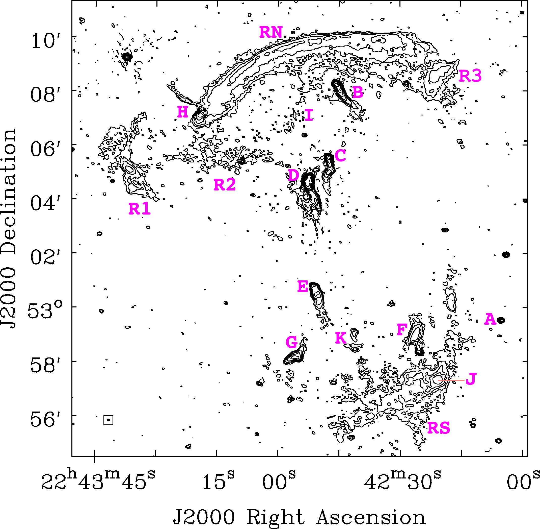
Figure 2: Source labels are adapted from Stroe et al. 2013. We label the patchy emission west of RN as R3. The contours are identical to those in Fig. 1.

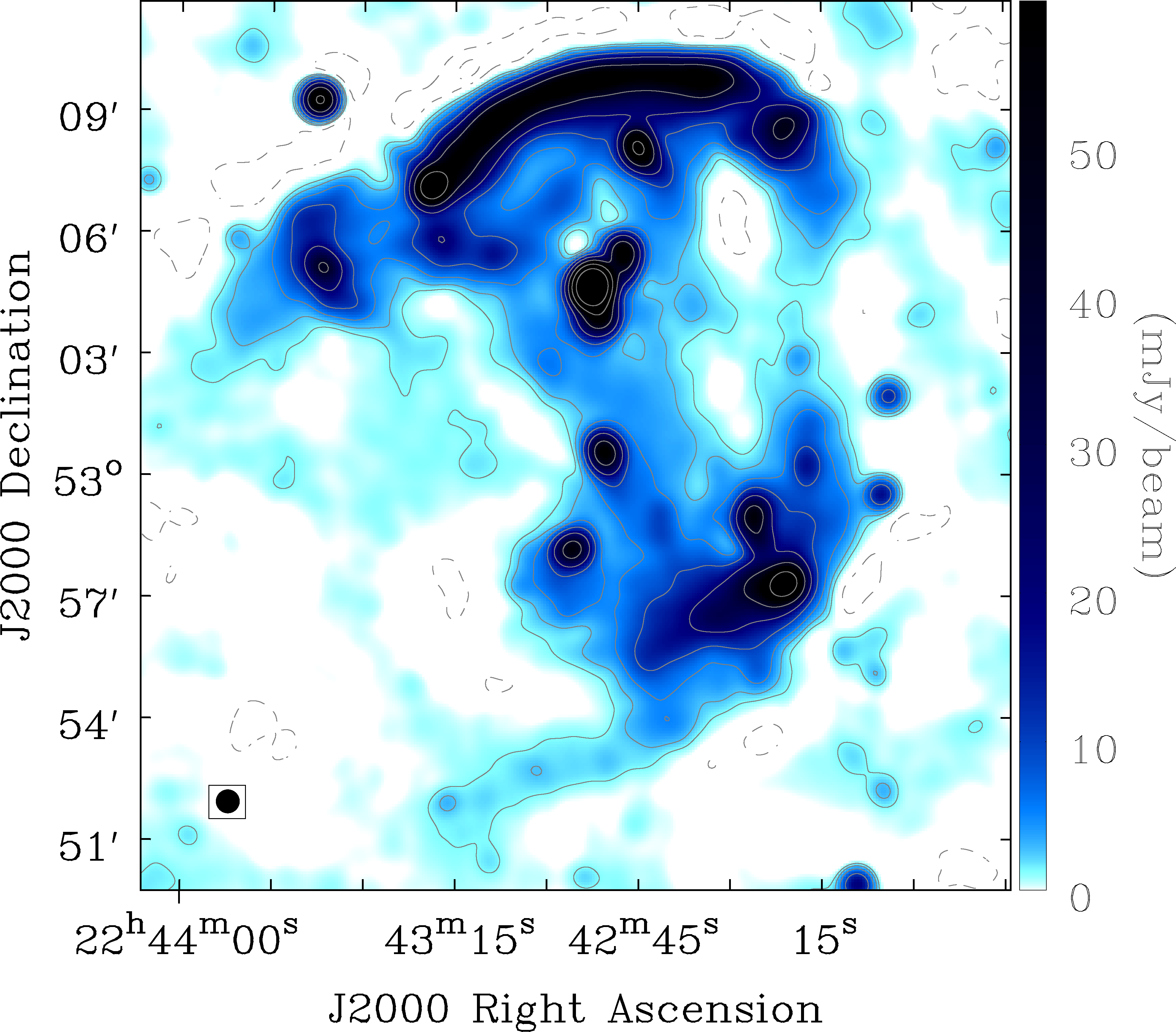
Figure 3: LOFAR total intensity low-resolution ($35\arcsec$, bottom left corner) image of CIZA2242. The radio contour levels are at $[-6,\,-3,\,3,\,6,\,12,\,24,\,48,\,96,\,192,\,384]\times\sigma_{\text{noise}}$ ($\sigma_{\text{noise}}=430\,\textrm{$\mu$Jy/beam}$). The negative contours are dashed lines.

Figure 4: LOFAR low-resolution ($35\arcsec$, bottom left corner) contours of CIZA2242 on top of Chandra X-ray image in the $0.5-7.0\,\text{keV}$ band (being smoothed to $6\arcsec$ resolution, Ogrean et al. 2014a). The radio contour levels are identical to those in Fig. 3 The blue dashed elliptical region is approximately the halo emission region. The green dotted region is over the source I.

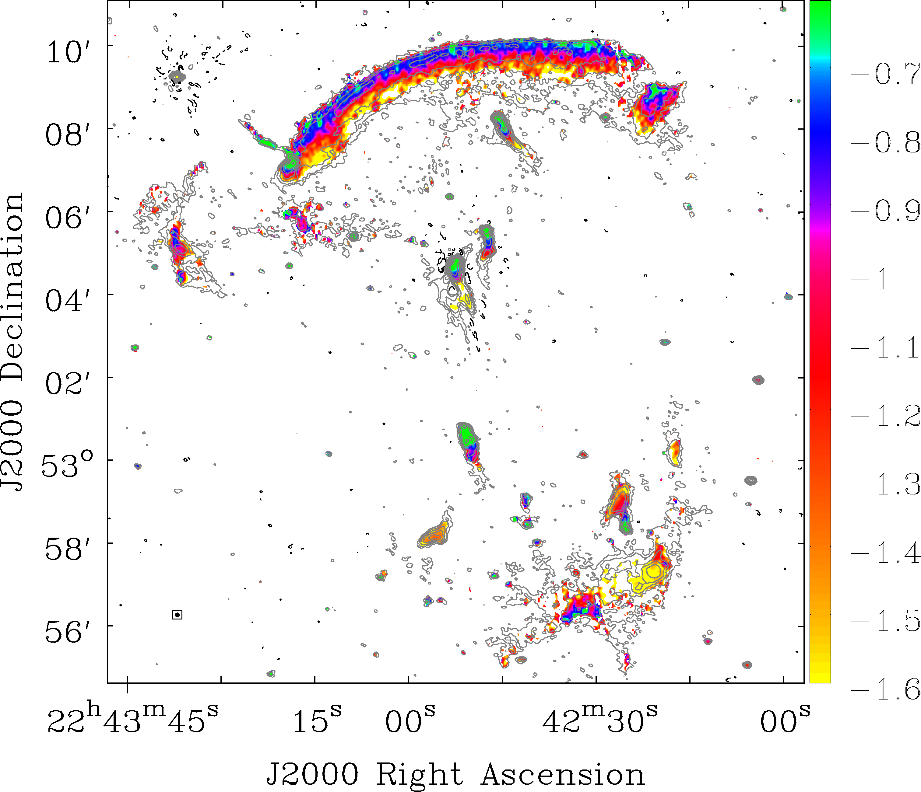
Figure 5: A $6.5\arcsec-$resolution spectral index map of CIZA2242 from 145 to 608 MHz. The LOFAR contours are identical to those in Fig. 1. The corresponding error map is shown in Fig. 16.

3.1 Northern relic

The northern relic (RN) is nicely mapped out in our LOFAR image (Fig. 1). Its morphology shows a familiar arc-like feature with a projected linear size of $1.9\,\mbox{Mpc}\times 230\,\mbox{kpc}$ (measured at $3\sigma_{\text{noise}}$ contours). The length of RN increases to $2.1\,\text{Mpc}$ when measured in the $35\arcsec$ map (Fig. 3). Its surface brightness has a sharp edge on the northern side and a more gradual decline on the southern side with additional diffuse emission north of source B. The integrated flux of RN (including the patchy emission in the west, source R3 in Fig. 2) is measured to be $1548.2\pm 4.6\,\mbox{mJy}$ within the $\geqslant 3\,\sigma_{\text{noise}}$ region. The flux increases by $4.6\%$ and $8.3\%$ for the $\geqslant 2\sigma_{\text{noise}}$ and $\geqslant 1\sigma_{\text{noise}}$ regions, respectively. The spectral index map between 145 and 608 MHz (Fig. 5) shows a clear steepening from the north towards the cluster centre, ranging roughly from $-0.80$ to $-1.40$. In Fig. 6, we plot the integrated fluxes of RN between 145 MHz and 2.3 GHz which were calculated within the LOFAR $\geqslant 3\sigma_{\text{noise}}$ region. The spectral index obtained from a weighted least-squares fitting of a power-law function to the RN fluxes at eight frequencies is $-1.11\pm 0.04$, which is consistent with the previous values of $-1.08\pm 0.05$ (van Weeren et al., 2010) and $-1.06\pm 0.04$ (Stroe et al., 2013).

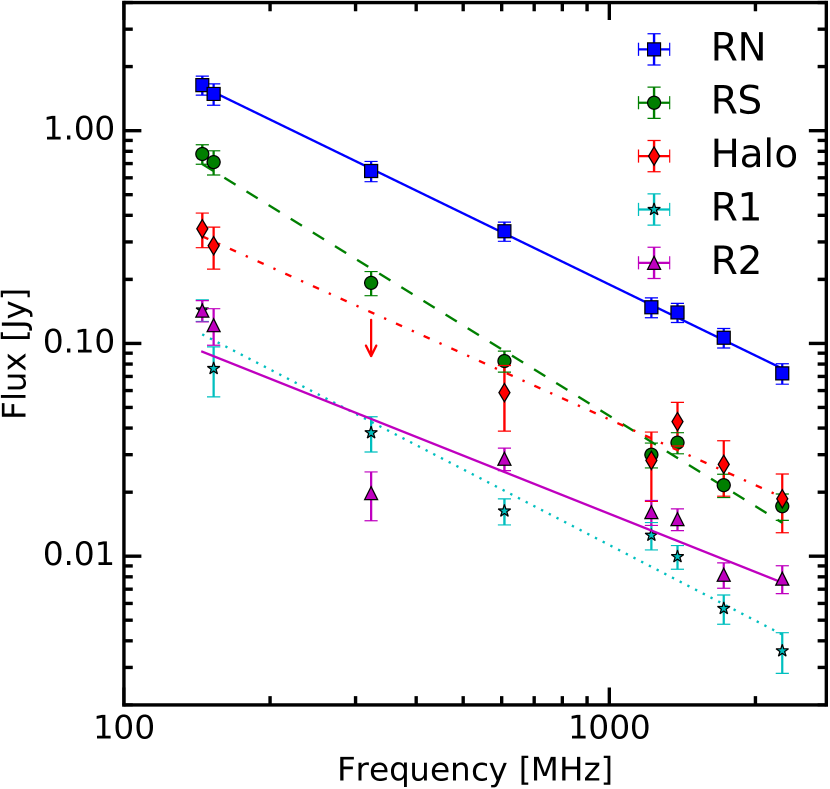
Figure 6: Integrated radio spectra of RN, RS, the halo, R1 and R2 from 145 MHz to 2.3 GHz including the LOFAR data points at the lowest frequency 145 MHz. The red downwards pointing arrow is the upper limit derived from the GMRT 323 MHz observations. The substantial scatter around the lines of best fit for the halo, R1 and R2 (e.g. compared with RN and RS) could be caused by the low signal to noise of the detections and the difficulty in precisely imaging large faint diffuse sources. Given the comparatively high surface brightness sensitivity of LOFAR, it is possible that the spectral indices for these sources is artificially steepened. The weighted best-fit integrated spectral indices are listed in Table 3. The integrated fluxes for the relics and halo are given in Table 5.

Towards the western side of RN, the main relic connects with source R3 via a faint bridge (a $3\sigma_{\text{noise}}$ detection). Towards the eastern side, RN is attached to source H, which is much brighter than other regions of the relic (the peak brightness is $30\,\mbox{mJy/beam}$, compared with a typical brightness $4.5\,\mbox{mJy/beam}$ in RN). The northern emission associated with source H has the expected morphology for an AGN.

In the post-shock central region of RN, an excess of emission was detected at a significance of up to $6\sigma_{\text{noise}}$ in front of source B. This emission has an arc-like shape with a projected linear size of $\sim 135\,\text{kpc}\times 500\,\mbox{kpc}$ within the $3\sigma_{\text{noise}}$ contours (Fig. 1). Interestingly, this feature was not detected in the post-shock eastern region of RN, where no tailed AGN are observed. The excess emission is more visible in the surface brightness profiles along the width of RN for the central and eastern regions in Fig. 7. Since the excess emission is located in front of source B and has a shock-like morphology, we speculate that this excess emission could be a bow shock generated by an interaction between the tailed AGN (source B) and the downstream relativistic electrons. We will present further analysis of this speculation in an upcoming paper.

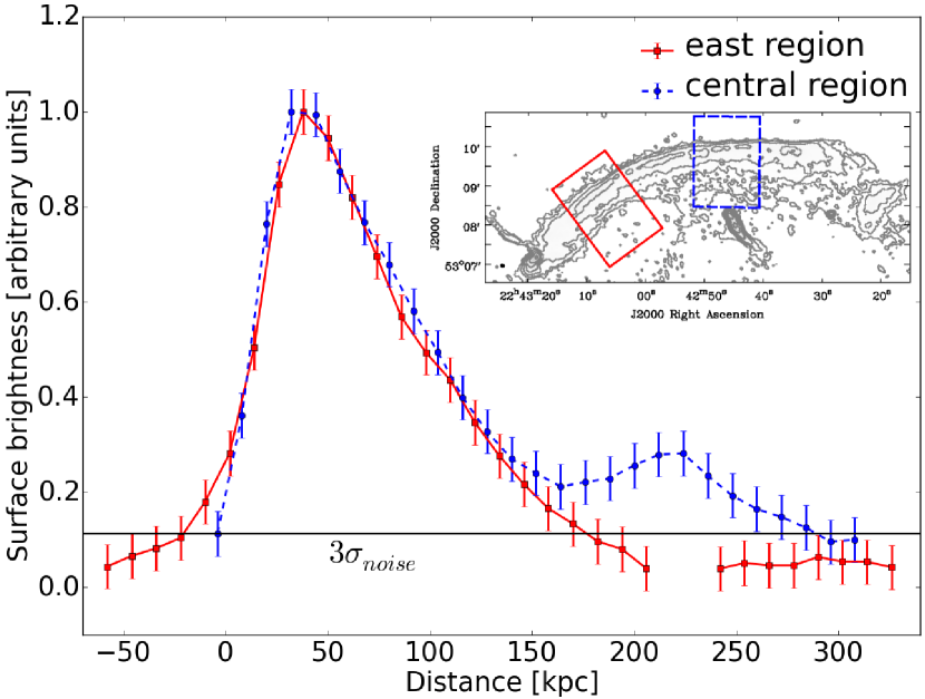
Figure 7: Surface brightness profiles (normalised) along the width of RN (in north-south direction) for the central (blue dashed) and east (red solid) regions (overlaid image). The data ($\geqslant 1\sigma_{\text{noise}}$) is averaged within $4\arcsec$ along the profile.

3.2 Southern relic

The southern relic (RS) is detected in our LOFAR map in Fig. 1 with a peak signal to noise of $\sim 20$. The distance between the outer edges of RN and RS is measured to be $2.8\,\text{Mpc}$ or $3.2\,\text{Mpc}$ in the $6.5\arcsec$ or $35\arcsec$ maps, respectively. The width of RS is wider in the central region with a size of $\sim 270\,\text{kpc}$ within the $\geqslant 3\sigma_{\text{noise}}$ region (Fig. 1). Within this central area the region labelled J covers $\sim 200\,\text{kpc}$ in radius and has substantially higher (threefold) surface brightness than the rest of the relic but no obvious counterpart in the optical data (see Fig. A.1. in Stroe et al. 2013).

The emission in the region of RS includes newly detected faint diffuse emission in the south-east region (Fig. 4 or Fig. 20). The size of RS in projection covers a maximum linear distance of $\sim 1.4\,\text{Mpc}$ as measured within the $3\sigma_{\text{noise}}$ contours in the $6.5\arcsec$ map. But its length when measured in the $35\arcsec$ map in Fig. 4 significantly increases to $\sim 2\,\text{Mpc}$ or $\sim 3\,\text{Mpc}$ when excluding or including the south-east emission. Within this new south-east region of emission, there are four optical sources which correspond to peaks in the radio emission as shown in Fig. 20. This faint emission could be the result of a collection of compact sources or it could be an in-falling filament at the cluster redshift. Unfortunately, we were unable to constrain the redshifts for the optical sources with the existing optical data. Additionally, faint diffuse emission is observed to extend south-westwards from the central region of RS (Fig. 1).

The zoom-in spectral index map of RS (eight frequencies from 145 MHz to 2.3 GHz) that is shown in Fig. 8 shows steepening towards the cluster centre. The spectral index drops approximately from $-0.85$ to $-1.40$ in the south-east region and from $-1.35$ to $-1.70$ in the north-west region. Similar trends are seen in the $145-608\,\text{MHz}$ spectral index map in Fig. 5. The north-west region of RS (Fig. 8) is dominated by diffuse emission in region J which has a very steep mean spectral index of $-2.0$. The region of flat spectrum in the south-east part (Fig. 8, left) has an L shape appearance and a steep spectrum of mean value of $-0.93\pm 0.10$. The west region of RS (Fig. 8, left) has an arc-like shape with an average spectral index of $-1.30\pm 0.04$ (excluding region J). We estimated the integrated spectral index for RS (within the LOFAR $\geqslant 3\sigma_{\text{noise}}$ region, including region J) to be $-1.41\pm 0.05$ (Fig. 6), which is steeper than the value of $-1.29\pm 0.04$ that was reported in Stroe et al. (2013).

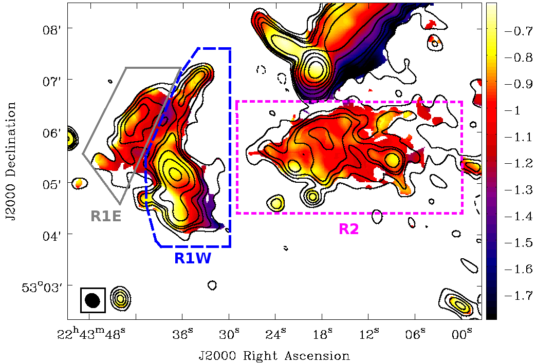
Figure 8: Zoom-in mid-resolution ($18\arcsec\times 16\arcsec$) spectral index maps of RS (left) and the eastern relics (right) from 145 MHz to 2.3 GHz (eight frequencies). The overlaid WSRT 1.4 GHz contours at the same resolution are levelled at $[3,6,9,12,24,48,96,192,384,768]\times\sigma_{\text{noise}}$($\sigma_{\text{noise}}=31.2\,\text{$\mu$Jy/beam}$).

3.3 Eastern relics

East of the cluster centre, slightly south, from RN (Fig. 1) are the relics R1 and R2, which were previously identified in Stroe et al. (2013). R1 consists of a thin narrow region. It is $\sim 630\,\mbox{kpc}$ long and oriented in the north-south direction. R1 has a bright region in the middle and patchy emission in the north-east. In Fig. 8 we show the eight-frequency spectral index distribution ($18\arcsec\times 16\arcsec$) of the eastern relics. Based on morphology and spectral index, we divided R1 into two regions: R1E in the north-east and R1W in the north-west (see Fig. 8). R1W has an arc-like morphology and shows spectral index steepening from approximately $-0.70$ to $-1.40$ towards the centre. The spectral index of R1E drops from approximately $-0.75$ to $-1.20$ in the same direction.

R2 has a physical size of $670\,\mbox{kpc}\times 270\,\mbox{kpc}$ with the major axis in the west-east direction (Fig. 8, right). Its spectral index between 145 MHz and 2.3 GHz remains approximately constant across its structure with a mean of $-0.95\pm 0.08$.

The integrated fluxes over the $\geqslant 3\sigma_{\text{noise}}$ region in the LOFAR $18\arcsec\times 16\arcsec$ image after masking out the compact sources were estimated to be $143.5\pm 8.3\text{\,mJy}$ and $142.5\pm 8.1\,\text{mJy}$ for R1 and R2, respectively. The integrated spectral indices between $145\,\text{MHz}$ and $2.3\,\text{GHz}$ are $-1.18\pm 0.06$ for R1 and $-0.91\pm 0.06$ for R2.

3.4 Radio halo

The halo was discovered by van Weeren et al. (2010) with WSRT observations at 1.4 GHz. Part of the emission was also seen in the GMRT 153 MHz image that was presented in Stroe et al. (2013). However, its flux and spectral properties have not been well studied. With our deep LOFAR image, we are able to characterise the radio halo as the large number of short baselines give LOFAR excellent sensitivity to cluster-scale emission. In Fig. 3, we show a low-resolution ($35\arcsec$) image of CIZA2242. The image shows diffuse emission connecting RN and RS with a significance up to $9\sigma_{\text{noise}}$ ($\sigma_{\text{noise}}=430\,\textrm{$\mu$Jy/beam}$). The emission covers an area of $1.8\,\text{Mpc}\times 830\,\text{kpc}$ with its major axis elongated in the north-south direction broadly following the Chandra X-ray emission that was mapped by Ogrean et al. (2014a).

The $145\,\text{MHz}$ flux of the radio halo was estimated from the LOFAR data in an elliptical region that was selected to cover the Chandra X-ray emission (Fig. 4). However, this region also hosts radio galaxies (i.e. source B, C, D, E, F, G, K) and diffuse emission from source I. We attempted to remove these contaminating sources from the halo flux estimation in two steps. In the first step, models of the radio galaxies were subtracted from the uv data. To obtain the radio galaxy models we created a LOFAR image using parameters that are similar to those used for the high-resolution ($6.5\arcsec$) image, except the inner uv cut was set to $0.4\,\text{k$\lambda$}$ instead of $0.2\,\text{k$\lambda$}$ (see Table 2 for the imaging parameters). Here the inner uv cut was used to filter out the large-scale emission from the halo to leave only the radio galaxies. The CLEAN components of these radio galaxies were subtracted from the uv data which were then imaged and smoothed to obtain a $35\arcsec$ image. The radio halo flux $S_{1}$ in the $\geqslant 3\sigma_{\text{noise}}$ elliptical region (blue dashed in Fig. 4), with source I masked, was measured from this $35\arcsec$ image. In the second step, the radio halo flux $S_{2}$ in the source I region (green dotted in Fig. 4) was estimated by extrapolating the halo flux $S_{1}$ using a scaling factor proportional to ratio of the areas (i.e. $\nicefrac{{\text{Area}_{S_{2}}}}{{\text{Area}_{S_{1}}}}=0.085$). We did not subtract source I from the uv data due to it having large-scale diffuse emission which is difficult to disentangle from the halo emission. Finally, the total halo flux ($S_{h}=S_{1}+S_{2}$) was estimated to be $S_{h}^{\text{145\,MHz}}=346\pm 64\,\text{mJy}$. Where we calculated the total error following Cassano et al. (2013) and took into account the flux scale uncertainty (i.e. $10\%$), image noise over the halo area and source subtraction uncertainty (i.e. $5\%$ of the total flux of the subtracted radio galaxies); additionally, we added an estimate of the uncertainty associated with the extrapolation of the halo flux in the source I region (i.e. assuming $10\%$). The source subtraction error of $5\%$ was estimated from the ratio of the post source subtraction residuals to the pre source subtraction flux of a nearby compact source (i.e. at RA=22:432:37, Dec=+53.09.16). Another uncertainty in the integrated flux is the area used for the integration. To assess the dependence on this we estimated the integrated radio flux within regions bounded by $\geqslant 2\sigma_{\text{noise}}$ and $\geqslant 1\sigma_{\text{noise}}$ within the elliptical region. We found the total halo flux at $145\,\text{MHz}$ remained approximately stable ($S_{h}^{145\,\text{MHz}}=362\pm 65\,\text{mJy}$ for $\geqslant 2\sigma_{\text{noise}}$ or $S_{h}^{145\,\text{MHz}}=371\pm 66\,\text{mJy}$ for $\geqslant 1\sigma_{\text{noise}}$).

Following a similar procedure we estimated the halo flux in the GMRT/WSRT data sets within the same region used for the LOFAR data. Unfortunately, due to the depth of the GMRT/WSRT observations, the halo emission was only partly detected in the GMRT 153, 608 MHz and WSRT 1.2, 1.4, 1.7, 2.3 GHz maps and undetected in the GMRT 323 MHz map. This may induce systematics in the spectral index estimate that deserve sensitive observations at higher frequencies in the future. In this paper we attempt our best following the approaches adopted in previous papers (e.g. van Weeren et al., 2016b; Stroe et al., 2013). First we used a common uv range (i.e. $0.2-50\,\text{k}\lambda$) and Briggs weighting (robust=0.5) when making the $35\arcsec$ images (see Subsec. 2.4). We also added an absolute flux scale uncertainty of $10\%$ to mitigate the impact on our conclusions due to possible missing flux in some observations. Due to the large uncertainties that are propagated in the above procedure (i.e. flux scale, image noise, source subtraction and extrapolation), we only created source subtracted low-resolution ($35\arcsec$) images. From these we estimated the inverse-variance weighted integrated spectrum which is plotted in Fig. 6. Using the combination of LOFAR, GMRT and WSRT data sets, the integrated spectral index from $145\,\text{MHz}$ to $2.3\,\text{GHz}$ of the radio halo was estimated to be $-1.03\pm 0.09$ and was found to remain approximately constant for different $\sigma_{\text{noise}}$ cuts on the area of integration (i.e. $1-3\sigma_{\text{noise}}$).

Table 3: Integrated spectral indices between 145 MHz and 2.3 GHz.

Source	$\alpha_{\text{int}}^{a}$	$\alpha_{\text{int}}^{b}$
RN	$-1.11\pm 0.04$	$-1.06\pm 0.04$
RS	$-1.41\pm 0.05$	$-1.29\pm 0.04$
R1	$-1.18\pm 0.06^{c}$	$-0.74\pm 0.07$
R2	$-0.91\pm 0.06$	$-0.90\pm 0.06$
Halo	$-1.03\pm 0.09^{d}$	N/A

^a: a flux scale uncertainty of $10\%$; ^b: Stroe et al. 2013; ^c: compact source was masked; ^d: compact source subtraction error of 5% and an uncertainty of 10% from the extrapolation of the halo emission in the source I region were added.

3.5 Tailed radio galaxies

Our LOFAR maps show that there are at least six tailed radio galaxies in CIZA2242 (i.e. source B, C, D, E, F, G in Fig. 1), a remarkably large number for any cluster. We mentioned in Sec. 1 that direct acceleration of thermal electrons by merger shocks is unable to explain the observed spectra and the efficiencies of electron acceleration for a number of relics (e.g. Akamatsu et al. 2015; Vazza et al. 2015; van Weeren et al. 2016b; Botteon et al. 2016). These problems could be solved with shock re-acceleration of fossil relativistic electrons. Tailed radio galaxies (e.g. Miley et al. 1972) are obvious reservoirs of such electrons, after activity in their nuclei has ceased or become weak. Indeed, some radio tails, such as 3C 129 (e.g. Lane et al. 2002) have Mpc-scale lengths and morphologies that bear striking resemblance to those of relics. Recent studies show evidence for particle re-acceleration of fossil electrons from radio galaxies in the radio relics of PLCKG287.0+32.9 (Bonafede et al. 2014) and Abell 3411-3412 (van Weeren et al. 2017). In the case of CIZA2242 there are bright radio galaxies located at the eastern extremity of RN (i.e. source H) and at the brightest central region of RS (i.e. source J). Whilst it remains unclear whether these radio galaxies are related to RN a scenario where fossil plasma could contribute to the emission in RN was previously discussed in Shimwell et al. (2015).

The combined systematic study of relics and tailed radio galaxies with radio sky surveys (e.g. Norris et al. 2017; Rottgering et al. 2011; Shimwell et al. 2017) may shed light on the role of tailed radio galaxies in the formation of radio relics, in particular in the case that radio relics originate from re-acceleration of fossil relativistic electrons and rather than from the acceleration of thermal plasma.

4 Discussion

CIZA2242 is one of the best studied merging clusters. In the radio band Stroe et al. (2013) carried out a detailed study of the cluster sources with GMRT/WSRT at frequencies ranging from 153 MHz to 2.3 GHz. Our LOFAR observations have produced higher-sensitivity, deeper images than the existing images at equivalent frequencies. In this section, we only discuss the new results obtained using the LOFAR images. We discuss below the discrepancy in the Mach numbers of RN and RS that were derived from X-ray and radio data, the characteristics of the post shock emission in RN, the eastern relic R1, and the radio halo.

4.1 Radio spectrum derived Mach numbers

The underlying particle-acceleration physics of shock waves closely relates to the shock Mach number and the observed spectra (e.g. Blandford & Eichler 1987; Donnert et al. 2016; Kang & Ryu 2016):

$$\mathcal{M}=\sqrt{\frac{2\alpha_{\text{inj}}-3}{2\alpha_{\text{inj}}+1}},$$ (4)

where the injection spectral index $\alpha_{\text{inj}}$ is related to the power-law energy distribution of relativistic electrons ($dN(p)/dp\propto p^{-\delta_{\text{inj}}}$, where $dN(p)$ is the electron number within momentum range $p$ and $p+dp$) via the relation $\alpha_{\text{inj}}=-(\delta_{\text{inj}}-1)/2$. For a simple planar shock model (Ginzburg & Syrovatskii, 1969) the injection index $\alpha_{\text{inj}}$ is flatter than the volume-integrated spectral index $\alpha_{\text{int}}$,

$$\alpha_{\text{inj}}=\alpha_{\text{int}}+0.5.$$ (5)

However, recent DSA test-particle simulations by Kang (2015a, b) indicate that this approximation (Eq. 5) breaks down for spherically expanding shock waves, due to shock compression and the injection electron flux gradually decreasing as the shock speed reduces in time. In the following Subsec. 4.1.1 and 4.1.2 we will estimate Mach numbers for the northern and southern shocks using the injection spectral indices that are measured from integrated spectra and resolved spectral index maps.

4.1.1 Mach numbers from integrated spectra

Using LOFAR data, together with existing radio data (van Weeren et al. 2010; Stroe et al. 2013), we measured volume-integrated spectral indices of $\alpha_{\text{int}}^{n}=-1.11\pm 0.04$ for RN and of $\alpha_{\text{int}}^{s}=-1.41\pm 0.05$ for RS. From that we derived injection indices of $\alpha_{\text{inj}}^{n}=-0.61\pm 0.04$ and $\alpha_{\text{inj}}^{s}=-0.91\pm 0.05$ (Eq. 5) and Mach numbers of $\mathcal{M}_{n}=4.4_{-0.6}^{+1.1}$ and $\mathcal{M}_{s}=2.4\pm 0.1$. For $\mathcal{M}_{n}$ our result is consistent with the findings of Stroe et al. (2013) ($4.58\pm{1.09}$, using colour-colour plots) and van Weeren et al. (2010) ($4.6_{-0.9}^{+1.3}$, using a $0.68-2.3\,\text{GHz}$ spectral index map). However, $\mathcal{M}_{s}$ is significantly smaller than that estimated in Stroe et al. (2013) ($2.80\pm 0.19$). Furthermore, there remains a discrepancy between the Mach numbers obtained from the integrated spectral index and those derived from X-ray data or spectral age modelling of radio data (Stroe et al. 2014; Akamatsu et al. 2015) (see Table 4).

4.1.2 Mach numbers from spectral index maps

An alternative way to obtain the injection index is to measure it directly from the shock front region in high resolution spectral index maps. Unfortunately , the precise thickness of the region in which the relativistic electrons are (re-)accelerated by the shock is unknown. However, given that the bulk velocity is approximately $905\,\text{km/s}$ in the downstream region (Stroe et al. 2014), the travel time for the electrons to cross a distance equivalent to the beam size of $6.5\arcsec$ ($22.5\,\text{Myrs}$) is $4-10$ times shorter than their estimated lifetime of $90-220\,\text{Myrs}$ (assuming the relativistic electrons are in the magnetic field $\sim\text{$\mu$G}$ and observed at the frequencies $150-610\,\text{MHz}$, see e.g. Donnert et al. 2016). Therefore, the shock (re-)accelerated relativistic electrons are not likely to lose a significant amount of their energy along the distance corresponding to the synthesized beam size; and the injection spectral index can be approximated from measurements at the shock front.

From the $6.5\arcsec$-resolution spectral index map in Fig. 5, we found $\alpha_{\text{inj}}^{n}=-0.81\pm 0.11$ within the shock front regions in Fig. 9. This injection index corresponds to $\mathcal{M}_{n}=2.7{}_{-0.3}^{+0.6}$, which is consistent with the X-ray and spectral age modelling derived Mach numbers (e.g. $2.90_{-0.13}^{+0.10}$ in Stroe et al. 2014 and $2.7_{-0.4}^{+0.7}$ in Akamatsu et al. 2015). A low Mach number like this may also be expected from structure formation simulations which typically have $2\apprle\mathcal{M}\apprle 4$ for internal shocks (Ryu et al. 2003; Pfrommer et al. 2006; Vazza et al. 2009). For RS, since the shock front location is detected furtherest from the cluster centre in the $35\arcsec$-resolution image (Fig. 12), we estimated the injection index from the lower-resolution map (see Fig. 9). We obtained an average value of the injection index of $\alpha_{\text{inj}}^{s}=-1.23\pm 0.22$ for RS. This is equivalent to a shock with Mach number of $\mathcal{M}_{s}=1.9_{-0.2}^{+0.3}$. Similarly to RN, the Mach number for RS that is measured directly at the shock front location in our resolved spectral index maps is in agreement with those measured with X-ray data whereas the Mach number derived from the integrated spectral index is $\sim 2\sigma$ higher. (e.g. $\mathcal{M}_{s}^{X}=1.7_{-0.3}^{+0.4}$ in Akamatsu et al. 2015, see table 4). It is noticed in Fig. 9 that the spectral indices along the shock front of RS have large variations from a minimum of $-1.53\pm 0.08$ (at $1.04\,\text{Mpc}$) to a maximum of $-0.91\pm 0.11$ (at $345\,\text{kpc}$), whereas the spectral indices at the shock front in RN remain approximately constant. Additionally, the spectral indices in the eastern side of RS (mean value of $\bar{\alpha}=-1.04\pm 0.12$) are flatter than those in the western side ($\bar{\alpha}=-1.43\pm 0.08$). This could imply that the southern shock propagated with different Mach numbers in different areas and that the shock travelled with a higher Mach number in the east. Another possibility is that due to the complex morphology of RS the regions, where the spectral indices were extracted, can host electron populations of different spectra along the line of sight.

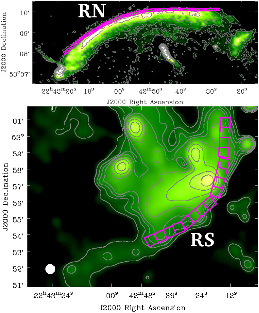
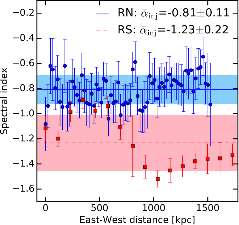
Figure 9: Spectral index profiles (right) for the flat spectrum regions of RN (top left) and RS (bottom left). The RN and RS profiles were extracted from the 145-608 MHz spectral index map (Fig. 5) and the 145 MHz - 2.3 GHz spectral index maps (Fig. 12, eight frequencies). The weighted means for RN ($\bar{\alpha}_{\text{inj}}^{n}=-0.81\pm 0.11$) and RS ($\bar{\alpha}_{\text{inj}}^{s}=-1.23\pm 0.22$) are plotted as horizontal lines (solid blue for RN and dashed red for RS). The errors of the weighted means are shown by the filled regions of the same colour.

4.1.3 Measurement uncertainty

The estimation of the injection indices from the volume-integrated and spatially-resolved spectra both have pros and cons. Firstly, while the accuracy of the former method does not depend on the spatial resolution of the observations nor the orientation of the merger axis, it may be affected by other sources, since the radio-integrated fluxes are calculated within the large volume. This argument was invoked to explain Mach number discrepancies in several other cases (e.g. Ogrean et al. 2014b; Trasatti et al. 2015; Itahana et al. 2015). It is also very likely a contributing factor in the measurements of RS where contaminating radio sources are present. Similarly, for RN the integrated fluxes might be also contaminated in this case by additional compression in the post-shock region that we discussed in Subsec. 3.1. To quantify this possible contamination, we estimated the integrated spectrum of RN masking out the affected compression region (Subsec. 3.1). We obtained $\alpha_{\text{int}}^{n}=-1.08\pm 0.04$ and $\mathcal{M}_{n}=5.1_{-0.9}^{+2.0}$ which is a higher Mach number than we obtained prior to removing the potentially contaminated region. Therefore, this potential contamination cannot explain the Mach number discrepancy. Secondly, as mentioned earlier, the $\alpha_{\text{inj}}-\alpha_{\text{int}}$ relation (Eq. 5) does not hold for spherically expanding shock waves such as RN and RS (Kang 2015a, b). Therefore, the volume-integrated spectra will not necessarily characterise the large-scale spherical shocks. This reason was used to explain the discrepancy of the radio and X-ray derived Mach numbers in the Toothbrush cluster (van Weeren et al. 2016b). Thirdly, the discrepancy might also come from micro-physics of the dynamics of relativistic particles, including diffusion across magnetic filaments, re-acceleration due to the interaction of CRs with magnetic field perturbations, adiabatic expansion and changes of the magnetic field strength in the downstream region (e.g. Donnert et al. 2016).

The injection indices that are directly estimated from spatially resolved spectral index maps might be less susceptible to contamination from embedded sources. However, for such measurements to be accurate it requires (i) the merger axis to be on/close to the plane of the sky to avoid the mixture of electron populations of different velocities along the line of sight, (ii) highly-resolved spectral index maps to minimise the convolution effect caused by the synthesised beam as this would artificially bias the injection indices, and (iii) precise alignment among the radio maps. In the case of CIZA2242, hydrodynamical binary-merger simulations by van Weeren et al. (2011) suggested that the merger axis is likely to be close to the plane of the sky (less than $10\degree$), and this was supported by Kang et al. (2012) who performed DSA simulations. Moreover, the surface brightness along the width of the eastern side of RN (Fig. 7, red curve) drops to $10\%$ of the peak value at a distance of $\sim 130\,\text{kpc}$ from the peak which is consistent with the simulated profiles with a small viewing angle in van Weeren et al. (2011). This implies that RN satisfies (i). However, due to the complex morphology of RS, the southern shock might be observed at a larger angle than the northern shock. To assess the impact of (ii), we calculated the injection indices at various spatial resolutions for RN. We made spectral index maps between $145$ and $608\,\text{MHz}$ at resolutions $6.5\arcsec,\,15\arcsec,\,30\arcsec$ and $45\arcsec$. The injection indices were measured at the shock-front and the sizes of the square regions used to extract the injection index are approximately equal to the beam size of the maps (see Fig. 9). We found that although the apparent injection locations are slightly shifted to the North for the lower-resolution maps, the values of the injection indices are weakly affected by the spatial resolution (see Fig. 10). Assuming a linear relation between $\alpha_{\text{inj}}$ and resolution $\theta$, we found $\alpha_{\text{inj}}^{n}=(-0.81\pm 0.10)+(-0.63\pm 2.78)\times 10^{-3}\theta[\text{arcsec}]$, which is consistent with the value of $\alpha_{\text{inj}}^{n}=-0.81\pm 0.11$ that we found in the $6.5\arcsec$-resolution map (Fig. 9). To account for (iii), we aligned the radio images when making spectral index maps using the procedure described in Subsec. 2.4. The GMRT $608\,\text{MHz}$ image was shifted a distance of $0.20\arcsec$ and $0.01\arcsec$ in RA and Dec axes, respectively. We found a small increase of $1\%$ in the Mach number when aligning the images.

A potential further complication is that X-ray derived Mach numbers also suffer from several systematic errors. As discussed in Akamatsu et al. (2017) (see Sect.4.3 of their paper), there are three main systematics, which prevents proper Mach number estimation from X-ray observations: (i) the projection effect, (ii) inhomogeneities in the ICM, and (iii) ion-electron non-equilibrium situation after the shock heating. In case of CIZA2242, the first point was already discussed above. Related to point (ii), van Weeren et al. (2011) revealed that it is less likely to be a large clumping factor because of the smooth shape of the relic. The third point would lead to the underestimation of the Mach numbers from X-ray observations. However, it is difficult to investigate this systematic without better spectra than those from the current X-ray spectrometer. The upcoming Athena satellite can shed new light on this point.

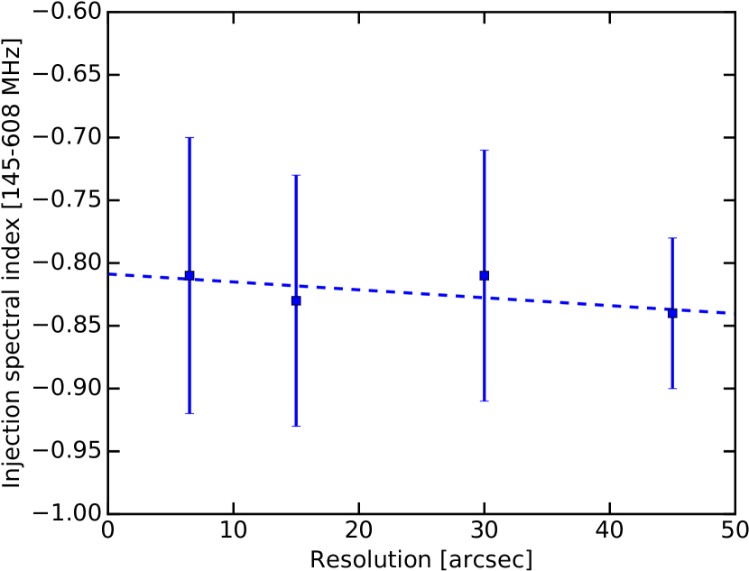
Figure 10: Injection spectral indices between 145 and 608 MHz of RN as measured at various spatial resolutions ($\alpha_{\text{inj}}=-0.81\pm 0.63\times 10^{-3}\theta_{[\text{arcsec}]}$). The regions where the indices were extracted are similar to those in Fig. 9.

Table 4: Spectral indices and Mach numbers for the shock waves.

Source	$\alpha_{\text{inj}}$	$\alpha_{\text{int}}$	$\mathcal{M}_{\textrm{inj}}$	$\mathcal{M}_{\textrm{int}}^{e}$	$\mathcal{M}^{X}$	$\mathcal{M}_{\textrm{ref}}$
RN	$-0.81\pm 0.11$	$-1.11\pm 0.04$	$2.7_{-0.3}^{+0.6}$	$4.4_{-0.6}^{+1.1}$	$2.7_{-0.4}^{+0.7}$ a	$4.6_{-0.9}^{+1.3}$ b, $4.58_{-1.09}^{+1.09}$ c, $2.90_{-0.13}^{+0.10}$ d
RS	$-1.23\pm 0.22$	$-1.41\pm 0.05$	$1.9_{-0.2}^{+0.3}$	$2.4_{-0.1}^{+0.1}$	$1.7_{-0.3}^{+0.4}$ a	$2.80_{-0.19}^{+0.19}$ c
R1	$-0.91\pm 0.14$	$-1.18\pm 0.06$	$2.4_{-0.3}^{+0.5}$	$3.5_{-0.4}^{+0.7}$	$2.5_{-0.2}^{+0.6}$	N/A

^a: Akamatsu et al. (2015), ^b: van Weeren et al. (2010), ^c: Stroe et al. (2013), ^d: Stroe et al. (2014), ^e: using Eq. 4 and 5.

4.2 Particle acceleration efficiency

The northern relic is known as one of the most luminous radio relics so far. But the low Mach number of $\mathcal{M}_{n}=2.7_{-0.3}^{+0.6}$ for RN (Subsec. 4.1) leads us to a question of acceleration efficiency that is required to explain such a luminous relic via shock acceleration of thermal electrons. The acceleration efficiency was defined as the fraction of the kinetic energy flux available at the shock that is converted into the supra-thermal and relativistic electrons (van Weeren et al. 2016b),

$$\eta_{e}=\frac{\epsilon_{e,\,\text{down}}v_{\text{down}}}{\Delta F_{\text{KE}}},$$ (6)

where $\epsilon_{e,\,\text{down}}$ and $v_{\text{down}}$ are the energy density and the velocity of the downstream accelerated electrons, respectively; $\Delta F_{\text{KE}}=0.5\rho_{\text{up}}v_{s,\,\text{up}}^{3}\left(1-\frac{1}{C^{2}}\right)$ is the kinetic energy available at the shock; here $\rho_{\text{up}}$ and $v_{s,\,\text{up}}$ are the upstream density and the shock speed, respectively; $C=\nicefrac{{\mathcal{M}^{2}(\gamma+1)}}{{[2+(\gamma-1)\mathcal{M}^{2}]}}$, here $\gamma$ is the adiabatic index of the gas and $\mathcal{M}$ is the shock Mach number. Following formula in Botteon et al. (2016), in Fig. 11 we report the efficiency of particle acceleration by the northern shock as a function of the magnetic field for the Mach number of $\mathcal{M}_{n}=2.7_{-0.3}^{+0.6}$ ($\alpha_{\text{inj}}=-0.81\pm 0.11$). We plotted the $1\sigma$ curves where $\mathcal{M}_{n}=2.4$ ($\alpha_{\text{inj}}=-0.92$, upper dashed) and $\mathcal{M}_{n}=3.3$ ($\alpha_{\text{inj}}=-0.70$, lower dashed), corresponding to the $1\sigma$ lower and upper boundaries, respectively. The magnetic field range ($\lesssim 20\,\text{$\mu$G}$) was selected to cover the values, $5-7\,\text{$\mu$G}$, in van Weeren et al. (2010). The relatively high efficiency of electron acceleration that should be postulated to explain the relic challenges the case of a shock with $\mathcal{M}_{n}<2.7$. In this case a population of pre-existing relativistic electrons in the upstream region of the shock should be assumed. However, in the DSA framework, it is still possible to accelerate electrons to relativistic energies directly from thermal pools in the case of $\mathcal{M}_{n}>2.7$. Future works will provide more constraints on this point.

Figure 11: Particle acceleration efficiency as a function of magnetic field for the northern relic. The solid curve is estimated for the Mach number of $\mathcal{M}_{n}=2.7$ ($\alpha_{\text{inj}}=-0.81$). The dashed curves are the $1\sigma$ uncertainties; the upper and lower dashed curves are for the $\mathcal{M}_{n}=2.4$ ($\alpha_{\text{inj}}=-0.92$) and $\mathcal{M}_{n}=3.3$ ($\alpha_{\text{inj}}=-0.70$) limits, respectively.

4.3 The radio halo

4.3.1 The spatial spectral variations

In Fig. 3 we show our LOFAR detection of the large-scale diffuse emission that connects RN and RS. This was previously reported in the WSRT 1.4 GHz observations and was interpreted as a radio halo by van Weeren et al. (2010). However, its physical characteristics, such as its flux and spectral index, have not been studied. With our deep LOFAR image (Fig. 3), we estimated the halo size within the $3\sigma_{\text{noise}}$ region to be $1.8\,\text{Mpc}\times 830\,\mbox{kpc}$ and the integrated flux to be $S_{h}=346\pm 64\,\textrm{mJy}$ (see Subsec. 3.4). The halo size in the north-south direction was measured between the northern and southern relic inner edges. The halo maintains its surface brightness, even in the regions that are least contaminated by the tailed AGNs, such as the regions east of source D or west of source E. The presence of the halo with elongated morphology connecting the north and south relics suggests a connection between the shock waves that are responsible for RN and RS. A comparable example of the morphological connection between radio relic and halo was observed in RX J0603.3+4214 where a giant radio relic at the northern edge of the cluster is connected to an elongated uniform brightness radio halo in the cluster centre (van Weeren et al. 2016b).

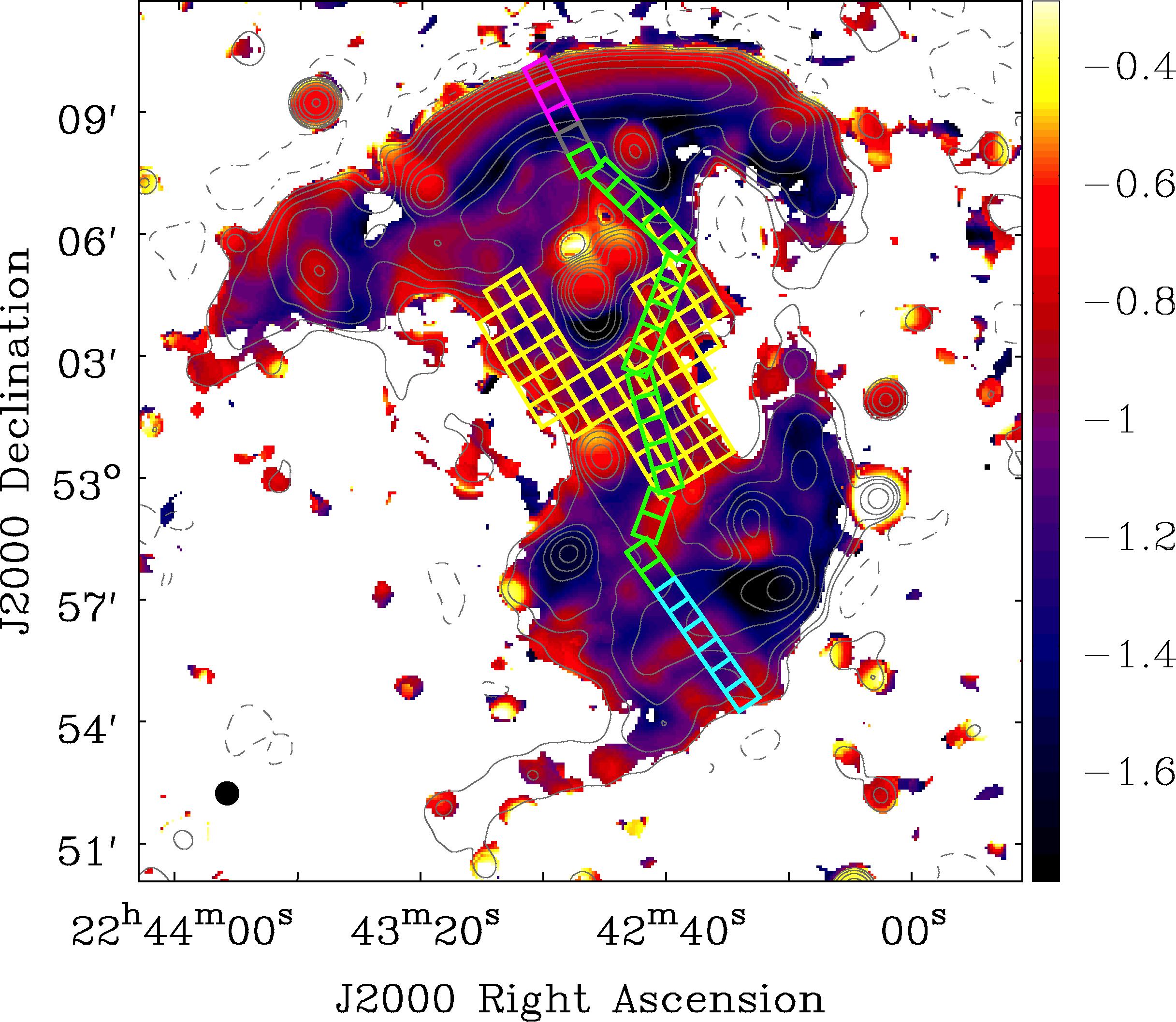
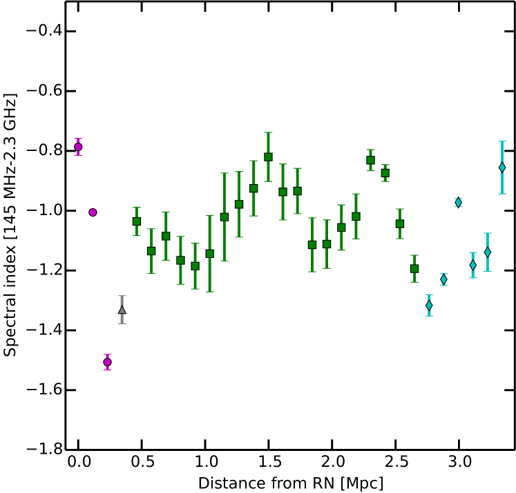
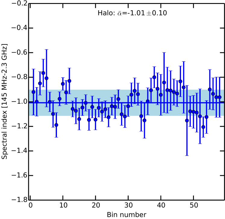
Figure 12: Left: A $35\arcsec$-resolution spectral index map between 145 MHz and 2.3 GHz (eight frequencies) including the regions where spectral indices were extracted. The square regions have a width of is $36\arcsec$ ($115\,\text{kpc}$). In the analysis of the spectral index variations, we did not take into account an absolute flux scale uncertainty of 10% as done for the $6.5\arcsec$ and $18\arcsec\times 16\arcsec$ maps in Fig. 5 and 8, respectively. Middle: Spectral index profile for the square (magenta, gray, green, cyan) regions in the left image. Right: The spectral indices in the square yellow regions over the selected radio halo area where the contamination from radio galaxies is minimised. The inverse-invariance weighted mean of the spectral indices for the halo regions (yellow squares ) is $-1.01\pm 0.10$.

We examined a spectral index profile (see Fig. 12, middle) across the north and south relics and the radio halo. We found that the spectral index steepens from $-0.79\pm 0.09$ at the northern shock front location to $-1.51\pm 0.08$ in the post-shock region ($230\,\text{kpc}$). It then flattens over a distance of $115\,\text{kpc}$ and remains approximately constant with a mean of $-1.03\pm 0.12$ over a distance of $2.5\,\mbox{Mpc}$. This mean spectral index of the halo is $-1.01\pm 0.10$ when measured in a $\sim\text{1 Mpc}^{2}$ region (i.e. yellow squares in Fig. 12, left) and is consistent with the integrated spectral index of $-1.03\pm 0.09$ that was estimated in Subsec. 3.4. Similarly, the spectral index profile across RS in the south-north direction (i.e. right-left direction in Fig. 12, middle) steepens from $-0.86\pm 0.08$ at the southern shock front to $-1.32\pm 0.05$ over a distance of $575\,\text{kpc}$ from the southern shock front (cyan diamonds at $\sim 2.7\,\text{Mpc}$ in Fig. 12, middle). After this steepening, the spectral indices flatten to $-0.83\pm 0.05$ over a distance of $460\,\text{kpc}$ (i.e. $2.2-2.7\,\text{Mpc}$ in Fig. 12, middle). However, it is possible that the spectral indices across RS and in the southern halo region are strongly effected by contaminating sources (i.e. K, J). Moreover, the spectral index variations in this area are at similar levels to those seen across the halo and therefore cannot be associated with the southern shock with certainty.

The spectral re-flattening of the emission downstream from the northern relic and into the northern part of the halo suggests particles have undergone re-acceleration. It is currently thought that giant radio halos trace turbulent regions in which particles are re-accelerated (see Brunetti & Jones 2014 for review). The fact that in several cases X-ray shocks coincide with edges of radio halos is suggestive of the possibility that these shocks can be sources of turbulence downstream (e.g. Markevitch 2010; Shimwell et al. 2014). More specifically shocks may inject compressive turbulence in the ICM and compressive turbulence is in fact used to model turbulent re-acceleration of electrons in radio halos in several papers (e.g. Brunetti & Lazarian 2007). In the case of CIZA2242 the electrons might be accelerated (or re-accelerated) at the northern shock front and lose energy downstream via radiative losses. However on longer times the shock-generated turbulence might decay to smaller scales and re-accelerate electrons inducing a flattening of the synchrotron spectrum. A similar scenario was invoked to explain the spatial behaviour of the spectral index in the post-shock region of RX J0603.3+4214 and the hole in the radio halo of Abell 2034 (van Weeren et al. 2016b and Shimwell et al. 2016). In RX J0603.3+4214, van Weeren et al. (2016b) also observed spectral steepening in the post-shock region from $-0.8$ at the shock front edge to $-2$ at the boundary of the relic and halo, which was followed by an approximately constant spectral index of $-1.06\pm 0.06$ across the Mpc-scale halo region. This suggests that in these, and potentially other clusters, we may be observing similar particle (re-)acceleration and ageing scenario.

The spectral indices over the large region of the radio halo, where the contaminating sources (i.e. B, C, D, E, F, G, K, I) are masked, are plotted in Fig. 12 (right). Following Cassano et al. (2013), we estimated the raw scatter (see Eq. 5 in Cassano et al. 2013) from the inverse-variance weighted mean to be $0.10$. From the weighted mean of the spectral index errors of $0.10$ unit that propagates from the image noise, the intrinsic scatter of $\sqrt{0.10^{2}-0.09^{2}}=0.04$ was obtained. The intrinsic scatter is smaller than the typical spectral index errors of $\Delta\alpha\thickapprox 0.13$ in the halo region (yellow squares in Fig. 12, left); hence, the measurements of the spectral indices in the halo region are close to the detection limit of our data. More precise spectral index measurements would therefore be required to study the physics of turbulence in the halo.

4.3.2 A comparison with radio-thermal correlations

Galaxy clusters statistically branch into two populations (Brunetti et al. 2007; Brunetti et al. 2009; Rossetti et al. 2011; Cassano et al. 2013; Cuciti et al. 2015; Yuan et al. 2015): dynamically disturbed systems host radio halos whose luminosity correlates with the X-ray luminosity and mass of the hosting systems, whereas in general relaxed systems do not host Mpc-scale halos at the sensitivity level of available observations. To examine whether or not the radio halo of CIZA2242 follows the relationship between radio luminosity and X-ray luminosity and mass of the hosting cluster, in Fig. 13 we plot the radio power $P_{1.4\,\text{GHz}}$ versus the X-ray luminosity $L_{500}$ in the $0.1-2.4\,\text{keV}$ energy band for a number of clusters that are given in Cassano et al. (2013); $L_{500}$ is the luminosity within the radius $R_{500}$ where the ICM matter density is 500 times the critical density of the Universe at redshift $z$. The radio power at 1.4 GHz for the CIZA2242 halo was estimated by extrapolating our measurements to be $P_{1.4\,\text{GHz}}=(3.5\pm 1.0)\times 10^{24}\,\text{W\,H}\text{z}^{-1}$ at the cluster redshift $z=0.192$ using the LOFAR 145 MHz integrated flux of $346\pm 64\,\text{mJy}$ and the integrated spectral index of $-1.03\pm 0.09$. Using the Chandra data (Ogrean et al. 2014a), we measured the X-ray luminosity of $L_{500}=(7.7\pm 0.1)\times 10^{44}\,\text{erg\,$\text{s}^{-1}$}$ for the $0.1-2.4\,\text{keV}$ energy band within a radius of $R_{500}=1.2\,\text{Mpc}$ at $z=0.192$. Fig. 13 shows that the CIZA2242 data point closely follows the $P_{1.4\,GHz}-L_{500}$ correlation (i.e. $P_{1.4\,\text{GHz}}[10^{24}\,\text{W\,H$z^{-1}$}]=10^{-1.52\pm 0.20}L_{500}{}^{2.11\pm 0.20}[10^{44}\,\text{erg\,$\text{s}^{-1}$}]$; BCES bisector best fit in Cassano et al. 2013).

Despite RN being amongst the most prominent radio relics known, the radio halo of CIZA2242 seems typical, with moderate radio power and X-ray luminosity in comparison with other radio halos (Fig. 13). Magneto-hydrodynamic simulations of re-acceleration of relativistic electrons via post-shock generated turbulence by Donnert et al. (2013) predict that the integrated spectrum of the halos is flatter in their early phase ($\lesssim 1\,\text{Gyr}$) and becomes steeper after $\sim 1.2\,\text{Gyrs}$ of core passage. With our current data, the radio halo of CIZA2242 has a relatively flat spectral index of $-1.03\pm 0.09$ and is among the flatter spectrum halos known (e.g. Feretti et al. 2012), implying that it has recently formed (e.g. also see our discussion in Subsec. 4.3.1). The early phase of the halo is further supported by binary cluster merger simulations by van Weeren et al. (2011) which suggested that the cluster is $1\,\text{Gyr}$ after core passage.

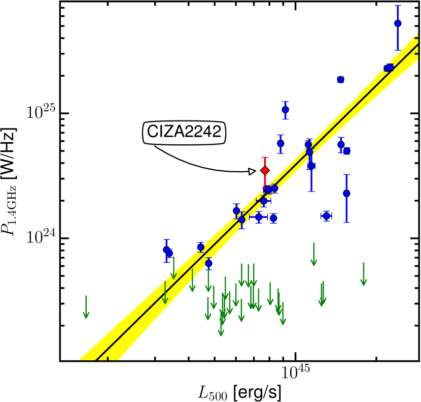
Figure 13: The scaling relation of the radio power $P_{1.4\,\text{GHz}}$ and X-ray luminosity $L_{500}$ for radio halos including CIZA2242 (red diamond). The list of the halos and the BCES bisector best fit $P_{1.4\,\text{GHz}}[10^{24}\,\text{W\,H$z^{-1}$}]=10^{-1.52\pm 0.21}\times L_{500}^{2.11\pm 0.20}[10^{44}\,\text{erg}\,\text{s}^{-1}]$ (without CIZA2242) were given in Cassano et al. (2013). The shadowed area is the $95\%$ confidence regions of the best-fit relation.

4.4 A newly detected eastern shock wave?

The steepening features in the spectral index of R1, reported in Subsec. 3.3, are likely due to the energy loses of relativistic electrons (e.g. synchrotron, IC emission). Additionally, the intensity maps (Fig. 1, 8 and 14, left) show emission with a sharp edge on the eastern side and a more gradual decline towards the western edge. These features are among the typical properties of radio emission associated with a shock wave. We speculate that R1E and R1W trace a complex shock wave that is propagating away from the cluster centre and that this shock (re-)energises two clouds of relic or aged electrons. In this scenario, the spectral steepening is more visible for R1E which implies that the shock wave is more on the plane of the sky in this region.. A $12\arcsec$ resolution map in Fig. 15 shows a bridge of low surface brightness (a $3\sigma_{\text{noise}}$ detection) that connects R1, R2, I, and RN. This suggests the origin of the eastern shock may be closely related to the cluster major merger. On our $18\arcsec\times 16\arcsec$ resolution map (Fig. 8, right) we measured the injection indices of $-0.89\pm 0.08$ for R1E and $-0.92\pm 0.12$ for R1W, the average of these injection indices is $-0.91\pm 0.14$ which is equivalent to a Mach number of $2.4_{-0.3}^{+0.5}$. Our estimation of the integrated spectral index of R1, within the LOFAR $>3\sigma_{\text{noise}}$ region, masking out the compact source in the central of R1W, is $-1.18\pm 0.06$. This is equivalent to a shock Mach number of $3.5_{-0.4}^{+0.7}$. Similarly to RN and RS, this Mach number is higher than the value that was calculated from the high resolution spectral index map.

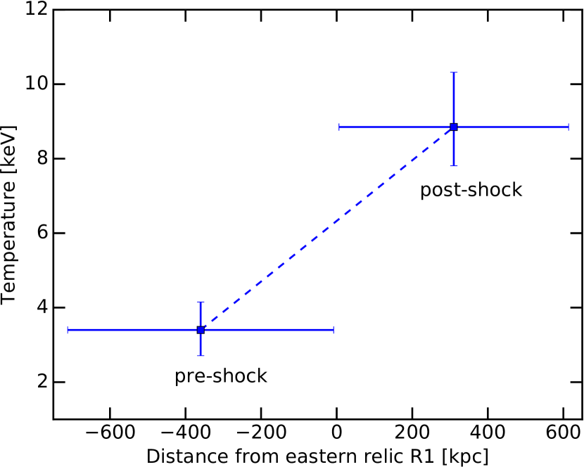
Figure 14: Left: Suzaku X-ray image for the north-east region of CIZA2242 overlaid with the WSRT 1.4 GHz contours (the first contour is $3\sigma_{\text{noise}}$, $\sigma_{\text{noise}}=30\,\mbox{$\mu$Jy/beam}$, beam size of $14\arcsec\times 11\arcsec$, and the next ones are spaced by 2.) The green rectangles are the pre- and post-shock regions of R1 within which the X-ray temperatures were extracted. Right: X-ray temperature for the corresponding regions in the left image.

To search for imprints of a shock in the X-ray data, we re-analysed the Suzaku data (Akamatsu et al. 2015) in the pre- and post-shock regions of R1 (see Fig. 14). We found an average temperature jump from $kT_{\text{pre}}=3.5{}_{-0.5}^{+0.8}\,\mbox{keV}$ to $kT_{\text{post}}=9.6{}_{-1.1}^{+1.5}\,\mbox{keV}$ from the pre- to post-shock region. This temperature jump of $6.1\,\text{keV}$ across the eastern relic is 2.4 times higher than a temperature decrease of $\sim 2.5\,\text{keV}$ over the eastern, slightly south region (i.e. centred at RA=22:43:24, DEC=+52.57.00) that is at a similar radial distance as the eastern relic but is devoid of radio emission (see Fig. 6 and 7 in Akamatsu et al. 2015). Therefore, the high temperature jump ($6.1\,\text{keV}$) is likely associated with the eastern relic. This X-ray temperature jump corresponds to a Mach number of $2.5_{-0.2}^{+0.6}$, which is consistent with our radio derived Mach numbers. The X-ray detection of a shock wave could be confirmed by measuring the discontinuity of the X-ray surface brightness profile. However, the existing Chandra and XMM-Newton data (Ogrean et al. 2013; Ogrean et al. 2014a; Akamatsu et al. 2015) do not have sufficient spatial coverage to detect the surface brightness discontinuity at the location of the eastern relic; and the Suzaku data has a limited spatial resolution of $2\arcmin$ which is insufficient for the surface brightness analysis. Our collection of radio and X-ray measurements provides compelling evidence that R1 is tracing another shock front in CIZA2242 that is propagating eastwards.

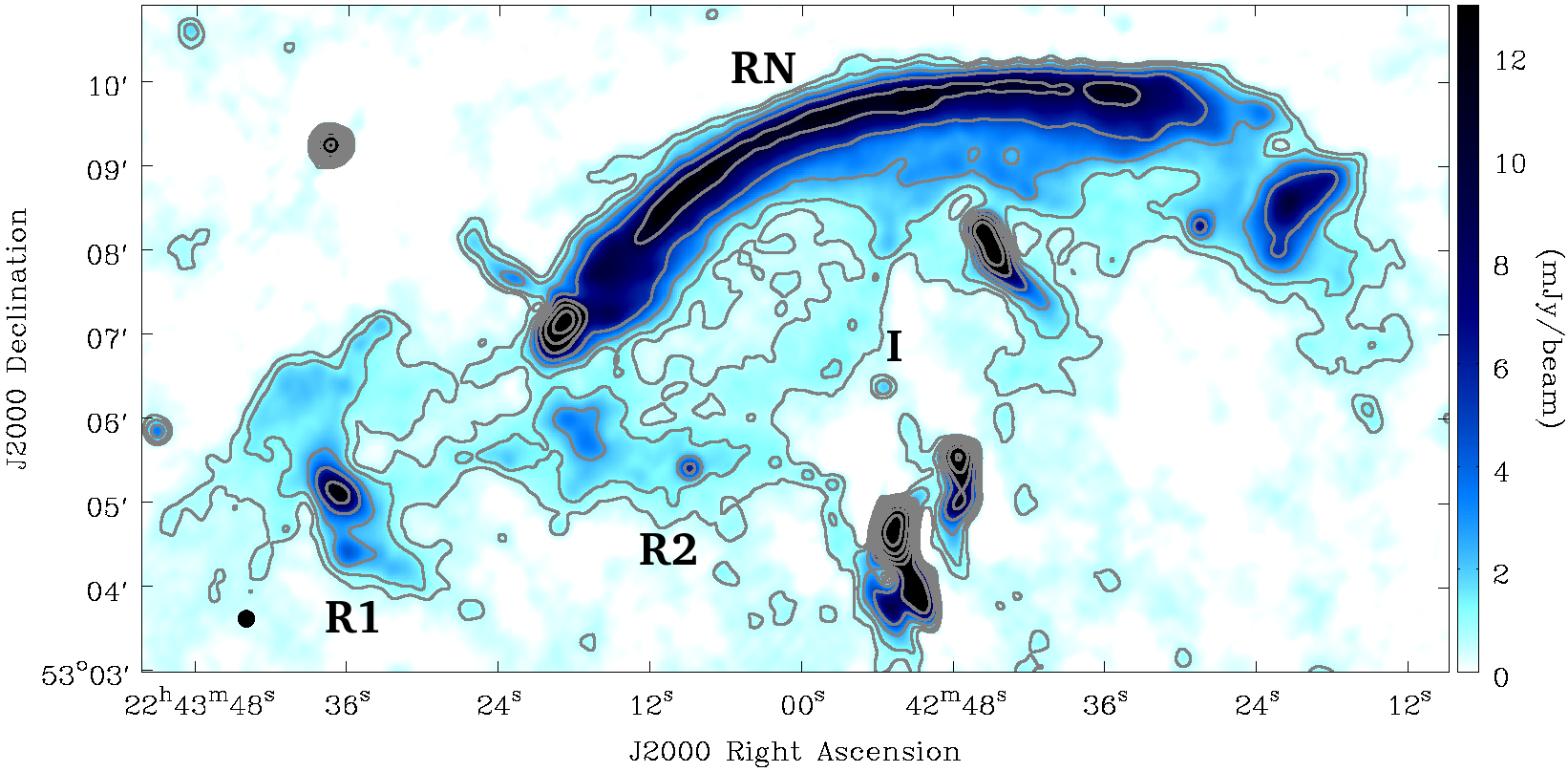
Figure 15: A zoom-in northern region of the LOFAR intensity image at $12\arcsec$ resolution. The first contour is at $3\sigma_{\text{noise}}$ ($\sigma_{\text{noise}}=210\,\text{$\mu$Jy/beam}$); the next ones is spaced by 2.

5 Conclusions

We have presented deep, high-fidelity LOFAR 145MHz images of CIZA2242, which have a resolution of $\sim 5\arcsec$ and a sensitivity of $140\,\text{$\mu$Jy/beam}$. The LOFAR data, in combination with the existing GMRT, WSRT, Suzaku and Chandra data were used to create spectral index maps of CIZA2242 at resolutions of $6.5\arcsec$, $18\arcsec\times 16\arcsec$ and $35\arcsec$. Below we summarise our main results.

• To investigate the long-standing discrepancy between X-ray and radio derived Mach numbers, we have measured injection spectral indices of $-0.81\pm 0.11$ and $-1.23\pm 0.22$ for the northern and southern relics, respectively. These correspond to Mach numbers of $\mathcal{M}_{n}=2.7_{-0.3}^{+0.6}$ and $\mathcal{M}_{s}=1.9_{-0.2}^{+0.3}$, and are in agreement with the Mach numbers derived from X-ray data (e.g. $\mathcal{M}_{n}=2.7_{-0.4}^{+0.7}$ and $\mathcal{M}_{s}=1.7_{-0.3}^{+0.4}$ in Akamatsu et al. 2015) and spectral age modelling study of the radio emission (e.g. $\mathcal{M}_{n}=2.9_{-0.13}^{+0.10}$ in Stroe et al. 2014).

• We have confirmed the existence of a radio halo and constrained its integrated flux ($346\pm 64\,\text{mJy}$) and its integrated spectral index ($-1.03\pm 0.09$, between 145 MHz and 2.3 GHz). We measured the radio halo power $P_{1.4\,\text{GHz}}=(3.5\pm 1.0)\times 10^{24}\,\text{W\,H}\text{z}^{-1}$ and the X-ray luminosity $L_{500}=(7.7\pm 0.1)\times 10^{44}\text{erg}\,\text{s}^{-1}$, which is close to the value expected from the $P_{1.4\,\text{GHz}}$-$L_{500}$ correlation. We have discussed a possible connection between the northern and southern relics and the halo, and have speculated that the formation of the halo may be driven by turbulence generated by the passing shock waves.

• In the radio source R1, in the north eastern region of the cluster, we found spectral steepening towards the cluster centre. A temperature jump from $3.5_{-0.5}^{+0.8}\,\text{keV}$ to $9.6_{-1.1}^{+1.5}\,\text{keV}$ was also detected at the location of the eastern relic R1 by re-analysing the existing Suzaku X-ray data. We suggest that R1 is an eastern relic that traces a shock wave that is propagating eastwards and (re-)energises the ICM electrons. We estimated an injection spectral index of $-0.91\pm 0.14$ and a Mach number of $\mathcal{M}_{e}=2.4_{-0.3}^{+0.5}$, which is consistent with our re-analysis of the Suzaku data from which we derived $\mathcal{M}_{e}^{X}=2.5_{-0.2}^{+0.6}$.

Appendix A Integrated fluxes for the radio relics and halo

Table 5 shows the integrated fluxes for the radio relics and halo in CIZA2242 that are plotted in Fig. 6. Note that the integrated fluxes for RN were reported in Stroe et al. (2015a); here we present the integrated fluxes from the images that were made with different CLEANing parameters (see Table 2).

Table 5: Integrated fluxes for the radio relics and halo in CIZA2242 in Fig. 6. The integrated fluxes for the relics were measured from the $18\arcsec\times 16\arcsec$ images, and the halo fluxes were estimated from the $35\arcsec$ images (see Table 2 for imaging parameters). The flux measurement errors for the relics were added absolute flux scale uncertainties of $10\%$ of the integrated fluxes. The flux error estimation for the radio halo was described in Subsec. 3.4.

Freq.	RN	RS	Halo	R1	R2
(MHz)	(mJy)	(mJy)	(mJy)	(mJy)	(mJy)
$145$	$1637\pm 168$	$777\pm 82$	$346\pm 64$	$144\pm 17$	$143\pm 16$
$153$	$1488\pm 171$	$711\pm 93$	$288\pm 64$	$76\pm 20$	$122\pm 24$
$323$	$646\pm 71$	$193\pm 25$	–a	$38\pm 7$	$20\pm 5$
$608$	$337\pm 35$	$83\pm 9$	$59\pm 20$	$16\pm 2$	$29\pm 3$
$1221$	$148\pm 16$	$30\pm 4$	$28\pm 10$	$13\pm 2$	$16\pm 2$
$1382$	$140\pm 14$	$34\pm 4$	$43\pm 10$	$10\pm 1$	$15\pm 2$
$1714$	$106\pm 11$	$22\pm 3$	$27\pm 8$	$6\pm 1$	$8\pm 1$
$2272$	$72\pm 8$	$17\pm 2$	$19\pm 6$	$4\pm 1$	$8\pm 1$

^a: a flux of 135 mJy was measured in the LOFAR $\geqslant 3\sigma_{\text{noise}}$ region of the GMRT 323 MHz $35\arcsec$ map. However, most of the flux comes from the residuals of the subtracted compact sources. We excluded the halo flux at the 323 MHz in the integrated spectral index estimation.

Appendix B Spectral index error maps

In Fig. 16-18, we show the error maps for the corresponding spectral index maps in Fig. 5, 8 and 12. The error estimation takes into account the individual image noise and a flux scale error of $10\%$, which is formulated in Eq. 2.

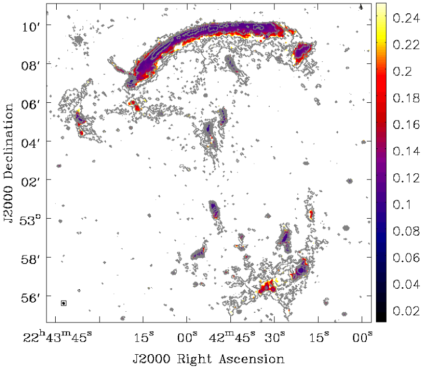
Figure 16: The corresponding spectral index error map for Fig. 5.

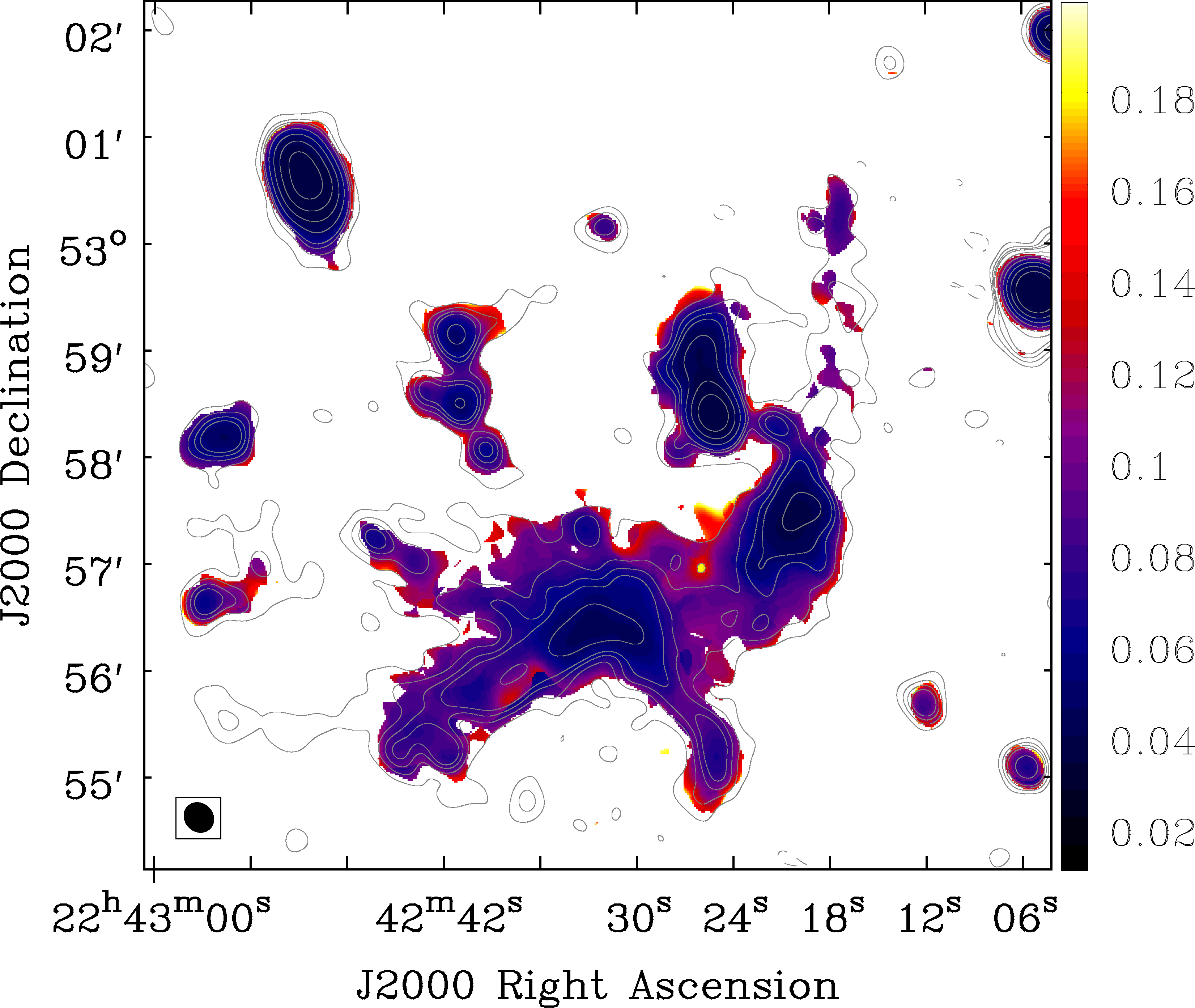
Figure 17: The corresponding spectral index error map for Fig. 8 (left).

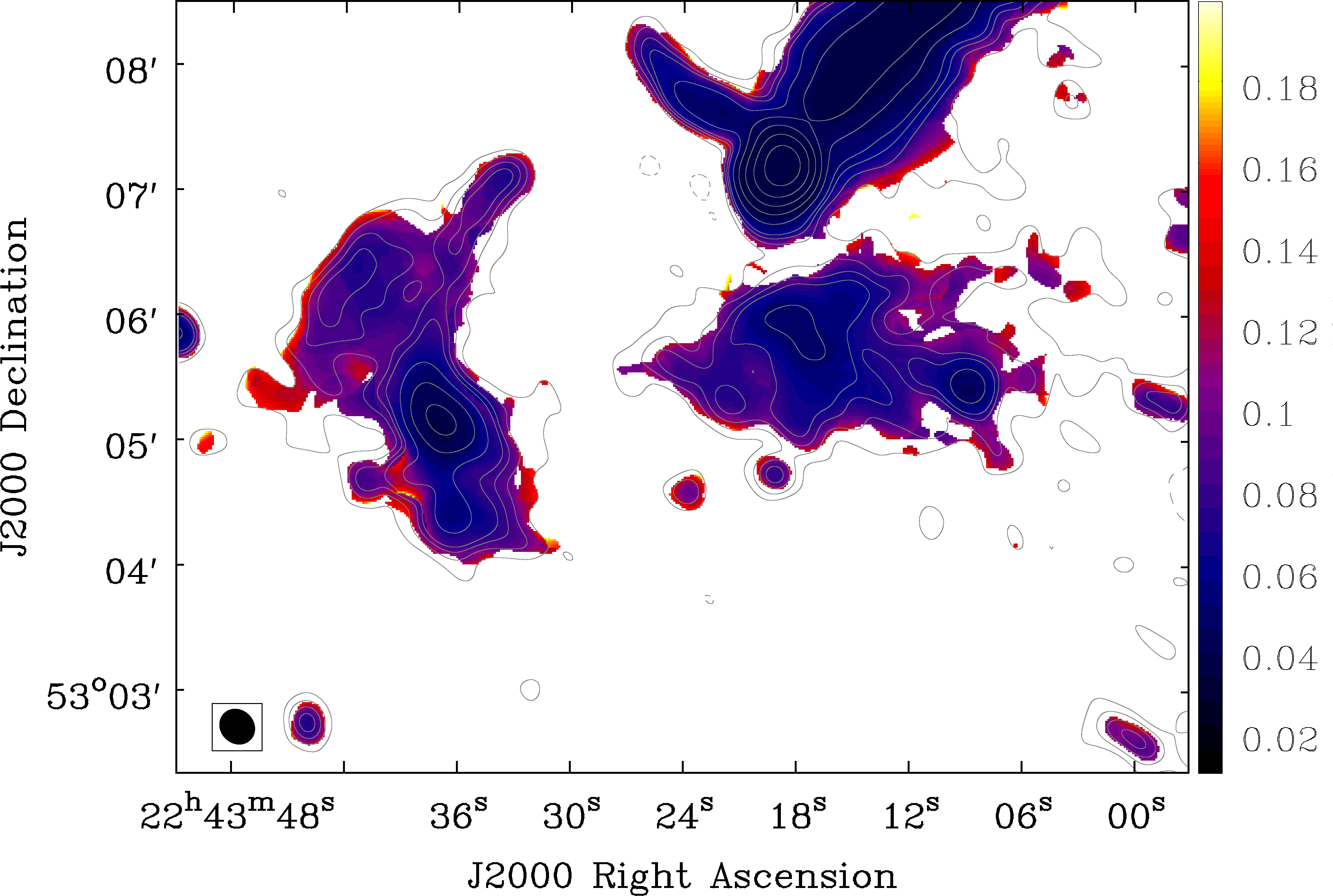
Figure 18: The corresponding spectral index error map for Fig. 8 (right).

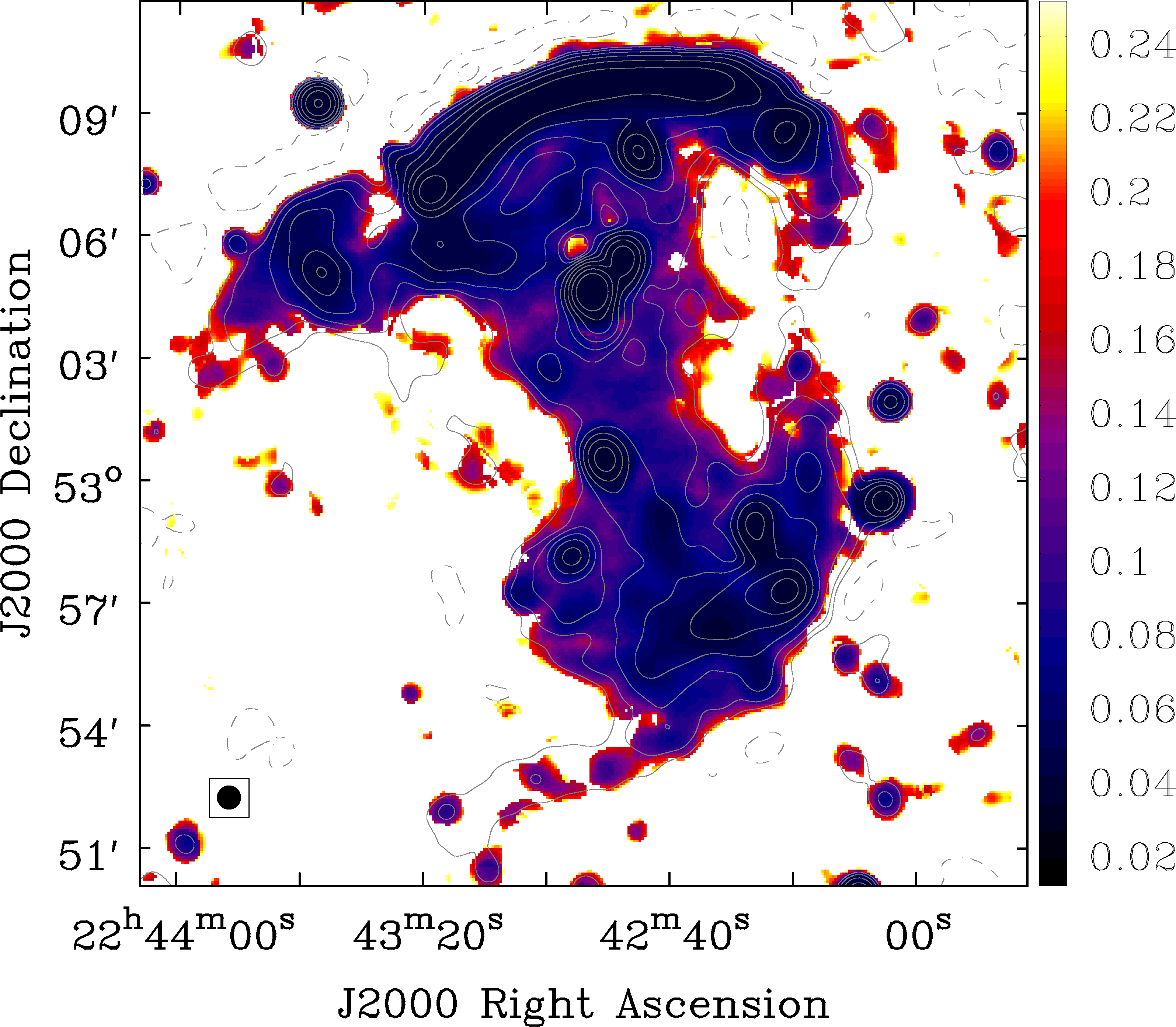
Figure 19: The corresponding spectral index error map for Fig. 12 (left).

Appendix C Eastern region of RS

A zoom-in optical image of the eastern region of RS is presented in Fig. 20.

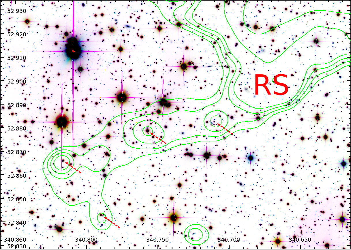
Figure 20: Optical image (Subaru g and i bands and CFHT r band, Stroe et al. 2015b; Jee et al. 2015) in the eastern side of RS. Four optical counterparts (red arrows) are detected at the locations of the radio emission peaks. The $35\arcsec$-resolution radio emission contours are levelled at $[3,\,4,\,5,\,6,\,12,\,24]\times\sigma_{\text{noise}}$.

References

- Ackermann et al. (2016) Ackermann M., et al., 2016, ApJ, 819, 149
- Akamatsu & Kawahara (2013) Akamatsu H., Kawahara H., 2013, PASJ, 65, 16
- Akamatsu et al. (2015) Akamatsu H., et al., 2015, A&A, 87, 1
- Akamatsu et al. (2017) Akamatsu H., et al., 2017, A&A, 600, A100
- Baars et al. (1977) Baars J. W. M., Genzel R., Pauliny-Toth I. I. K., Witzel A., 1977, A&A, 61, 99
- Bell & R. (1978) Bell A. R., R. A., 1978, MNRAS, 182, 147
- Blandford & Eichler (1987) Blandford R., Eichler D., 1987, Phys. Rep., 154, 1
- Blasi & Colafrancesco (1999) Blasi P., Colafrancesco S., 1999, Astropart. Phys., 12, 169
- Bonafede et al. (2014) Bonafede A., et al., 2014, ApJ, 785, 1
- Botteon et al. (2016) Botteon A., Gastaldello F., Brunetti G., Kale R., 2016, MNRAS, 000, 1
- Brown & Rudnick (2011) Brown S., Rudnick L., 2011, MNRAS, 412, 2
- Bruggen et al. (2012) Bruggen M., Bykov A., Ryu D., Rottgering H., Brüggen M., Bykov A., Ryu D., Röttgering H., 2012, Space Sci. Rev., 166, 187
- Brunetti & Jones (2014) Brunetti G., Jones T. W., 2014, Int. J. Mod. Phys. D, 23, 1430007
- Brunetti & Lazarian (2007) Brunetti G., Lazarian A., 2007, MNRAS, 378, 245
- Brunetti & Lazarian (2011) Brunetti G., Lazarian A., 2011, MNRAS, 412, 817
- Brunetti et al. (2001) Brunetti G., Setti G., Feretti L., Giovannini G., 2001, MNRAS, 320, 365
- Brunetti et al. (2004) Brunetti G., Blasi P., Cassano R., Gabici S., 2004, MNRAS, 350, 1174
- Brunetti et al. (2007) Brunetti G., Venturi T., Dallacasa D., Cassano R., Dolag K., Giacintucci S., Setti G., 2007, ApJ, 670, L5
- Brunetti et al. (2009) Brunetti G., Cassano R., Dolag K., Setti G., 2009, A&A, 669, 661
- Brunetti et al. (2012) Brunetti G., Blasi P., Reimer O., Rudnick L., Bonafede A., Brown S., 2012, MNRAS, 426, 956
- Cassano et al. (2013) Cassano R., et al., 2013, ApJ, 777, 141
- Cornwell (2008) Cornwell T. J., 2008, IEEE J. Sel. Top. Signal Process., 2, 793
- Cornwell et al. (2005) Cornwell T., Golap K., Bhatnagar S., 2005, in Shopbell P., Britton M., Ebert R., eds, Astronomical Society of the Pacific Conference Series Vol. 347, Astron. Data Anal. Softw. Syst. XIV. p. 86
- Cuciti et al. (2015) Cuciti V., Cassano R., Brunetti G., Dallacasa D., Kale R., Ettori S., Venturi T., 2015, A&A, 580, A97
- Dawson et al. (2015) Dawson W. a., et al., 2015, ApJ, 805, 143
- Dennison (1980) Dennison B., 1980, ApJ, 239, L93
- Dolag & Ensslin (2000) Dolag K., Ensslin T. A., 2000, A&A, 362, 151
- Donnert et al. (2013) Donnert J., Dolag K., Brunetti G., Cassano R., 2013, MNRAS, 429, 3564
- Donnert et al. (2016) Donnert J. M. F., Stroe A., Brunetti G., Hoang D., Roettgering H., 2016, MNRAS, 462, 2014
- Drury (1983) Drury L. O., 1983, Reports Prog. Phys., 46, 973
- Enßlin et al. (1998) Enßlin T. A., Biermann P. L., Klein U., Kohle S., 1998, A&A, 409, 395
- Enßlin et al. (2001) Enßlin T. A. T., Gopal-Krishna Gopal K., 2001, A&A, 366, 26
- Feretti et al. (2012) Feretti L., Giovannini G., Govoni F., Murgia M., 2012, Astron. Astrophys. Rev., 20, 54
- Ginzburg & Syrovatskii (1969) Ginzburg V., Syrovatskii S., 1969, The origin of cosmic rays
- Gizani et al. (2005) Gizani N. A. B., Cohen A., Kassim N. E., 2005, MNRAS, 358, 1061
- Hoeft et al. (2011) Hoeft M., et al., 2011, J. Astrophys. Astron., 32, 509
- Itahana et al. (2015) Itahana M., Takizawa M., Akamatsu H., Ohashi T., Ishisaki Y., Kawahara H., van Weeren R. J., 2015, Publ. Astron. Soc. Japan, 67, 113
- Jee et al. (2015) Jee M. J., et al., 2015, ApJ, 802, 46
- Jeltema & Profumo (2011) Jeltema T. E., Profumo S., 2011, ApJ, 728, 53
- Kang (2015a) Kang H., 2015a, J. Korean Astron. Soc., 48, 9
- Kang (2015b) Kang H., 2015b, J. Korean Astron. Soc., 48, 155
- Kang & Ryu (2011) Kang H., Ryu D., 2011, ApJ, 734, 18
- Kang & Ryu (2016) Kang H., Ryu D., 2016, ApJ, 823, 13
- Kang et al. (2012) Kang H., Ryu D., Jones T. W., 2012, Astrophys. J., 756, 97
- Kocevski et al. (2007) Kocevski D. D., Ebeling H., Mullis C. R., Tully R. B., 2007, ApJ, 662, 224
- Lane et al. (2002) Lane W. M., Kassim N. E., Ensslin T. A., Harris D. E., Perley R. A., 2002, ApJ, 123, 2985
- Markevitch (2010) Markevitch M., 2010, Twelfth Marcel Grossmann Meet. Gen. Relativ., p. 14
- Markevitch et al. (2005) Markevitch M., Govoni F., Brunetti G., Jerius D., 2005, ApJ, 627, 733
- McMullin et al. (2007) McMullin J., Waters B., Schiebel D., Young W., Golap K., 2007, in Shaw R., Hill F., Bell D., eds, Astronomical Society of the Pacific Conference Series Vol. 376, Astron. Data Anal. Softw. Syst. XVI. p. 127
- Miley et al. (1972) Miley G., Perola G., van der Kruit P., van der Laan H., 1972, Nature, 237, 269
- Miniati (2015) Miniati F., 2015, ApJ, 800, 60
- Norris et al. (2017) Norris R. P., et al., 2017, Publ. Astron. Soc. Aust., 28, 215
- Offringa et al. (2012) Offringa A. R., van de Gronde J. J., Roerdink J. B. T. M., 2012, A&A, 539, A95
- Offringa et al. (2014) Offringa A. R., et al., 2014, MNRAS, 444, 606
- Ogrean et al. (2013) Ogrean G. a., Bruggen M., Rottgering H., Simionescu A., Croston J. H., van Weeren R., Hoeft M., 2013, MNRAS, 429, 2617
- Ogrean et al. (2014a) Ogrean G. a., et al., 2014a, MNRAS, 440, 3416
- Ogrean et al. (2014b) Ogrean G. A., et al., 2014b, MNRAS, 443, 2463
- Pandey et al. (2009) Pandey V. N., Zwieten J. E. V., Bruyn A. G. D., Nijboer R., 2009, "The Low-Frequency Radio Universe", ASP Conf. Ser., 407, 384
- Petrosian (2001) Petrosian V., 2001, ApJ, 557, 560
- Pfrommer et al. (2006) Pfrommer C., Springel V., Ensslin T. A., Jubelgas M., 2006, MNRAS, 367, 113
- Pinzke et al. (2016) Pinzke A., Oh S. P., Pfrommer C., 2016, arXiv, pp 1–6
- Rau & Cornwell (2011) Rau U., Cornwell T. J., 2011, A&A, 532, A71
- Rich et al. (2008) Rich J. W., de Blok W. J. G., Cornwell T. J., Brinks E., Walter F., Bagetakos I., Kennicutt R. C., 2008, ApJ, 136, 2897
- Roettiger et al. (1999) Roettiger K., Burns J. O., Stone J. M., 1999, ApJ, 518, 603
- Rossetti et al. (2011) Rossetti M., Eckert D., Cavalleri B. M., Molendi S., Gastaldello F., Ghizzardi S., 2011, A&A, 532, A123
- Rottgering et al. (2011) Rottgering H., et al., 2011, J. Astrophys. Astron., 32, 557
- Ryu et al. (2003) Ryu D., Kang H., Hallman E., Jones T., 2003, ApJ, 593, 599
- Scaife & Heald (2012) Scaife A. M. M., Heald G. H., 2012, Mon. Not. R. Astron. Soc. Lett., 423, 30
- Shimwell et al. (2014) Shimwell T. W., Brown S., Feain I. J., Feretti L., Gaensler B. M., Lage C., 2014, MNRAS, 440, 2901
- Shimwell et al. (2015) Shimwell T. W., Markevitch M., Brown S., Feretti L., Gaensler B. M., Johnston-Hollitt M., Lage C., Srinivasan R., 2015, MNRAS, 449, 1486
- Shimwell et al. (2016) Shimwell T. W., et al., 2016, MNRAS, 459, 277
- Shimwell et al. (2017) Shimwell T. W., et al., 2017, A&A, 598, A104
- Stroe et al. (2013) Stroe a., van Weeren R. J., Intema H. T., Röttgering H. J. A., Brüggen M., Hoeft M., J V. W. R., 2013, A&A, 555, A110
- Stroe et al. (2014) Stroe A., Harwood J. J., Hardcastle M. J., Röttgering H. J. A., 2014, MNRAS, 445, 1213
- Stroe et al. (2015a) Stroe A., et al., 2015a, MNRAS, 000, 2402
- Stroe et al. (2015b) Stroe A., et al., 2015b, MNRAS, 450, 646
- Tasse et al. (2013) Tasse C., van der Tol S., van Zwieten J., van Diepen G., Bhatnagar S., 2013, A&A, 553, 13
- Trasatti et al. (2015) Trasatti M., Akamatsu H., Lovisari L., Klein U., Bonafede A., Bruggen M., Dallacasa D., Clarke T., 2015, A&A, 575, A45
- Vazza et al. (2009) Vazza F., Brunetti G., Kritsuk A., Wagner R., Gheller C., Norman M., 2009, A&A, 504, 33
- Vazza et al. (2015) Vazza F., Eckert D., Brüggen M., Huber B., Bruggen M., Huber B., 2015, MNRAS, 451, 2198
- Williams et al. (2016) Williams W. L., et al., 2016, MNRAS, 460, 2385
- Yuan et al. (2015) Yuan Z. S., et al., 2015, ApJ, 813, 77
- Zandanel & Ando (2014) Zandanel F., Ando S., 2014, MNRAS, 440, 663
- van Haarlem et al. (2013) van Haarlem M. P., et al., 2013, A&A, 2, 1
- van Weeren et al. (2010) van Weeren R. J., Rottgering H. J. A., Bruggen M., Hoeft M., Röttgering H. J. A., Brüggen M., Hoeft M., 2010, Science (80-. )., 330, 347
- van Weeren et al. (2011) van Weeren R. J., Brüggen M., Röttgering H. J. A., Hoeft M., 2011, MNRAS, 418, 230
- van Weeren et al. (2013) van Weeren R. J., et al., 2013, ApJ, 769, 101
- van Weeren et al. (2016a) van Weeren R. J., et al., 2016a, ApJS, 223, 2
- van Weeren et al. (2016b) van Weeren R. J., et al., 2016b, ApJ, 818, 204
- van Weeren et al. (2017) van Weeren R. J., et al., 2017, Nat. Astron., 1, 0005
- van der Tol et al. (2007) van der Tol S., Jeffs B., van der Veen A.-J., 2007, IEEE Trans. Signal Process., 55, 4497