The role of quantum coherence in dimer and trimer excitation energy transfer

Abstract

Recent progress in resource theory of quantum coherence has resulted in measures to quantify coherence in quantum systems. Especially, the $l_{1}$-norm and relative entropy of coherence have been shown to be proper quantifiers of coherence and have been used to investigate coherence properties in different operational tasks. Since long-lasting quantum coherence has been experimentally confirmed in a number of photosynthetic complexes, it has been debated if and how coherence is connected to the known efficiency of population transfer in such systems. In this study, we investigate quantitatively the relationship between coherence, as quantified by $l_{1}$-norm and relative entropy of coherence, and efficiency, as quantified by fidelity, for population transfer between end-sites in a network of two-level quantum systems. In particular, we use the coherence averaged over the duration of the population transfer in order to carry out a quantitative comparision between coherence and fidelity. Our results show that although coherence is a necessary requirement for population transfer, there is no unique relation between coherence and the efficiency of the transfer process.

1 Introduction

The idea of using and quantifying coherence as a resource was first introduced by Åberg [1]. Later, Baumgratz et al. [2] further developed the resource theory and framework for quantification of quantum coherence. Their approach is directly analogous to entanglement theory; the resource states correspond to entangled states while the free (incoherent) states correspond to separable states in entanglement theory. Incoherent operations are those which map the set of free states back to itself, similar to the preservation of separable states under local operations and classical communication (LOCC) in entanglement theory.

Quantification of quantum coherence, which makes it possible to distinguish different quantum states in terms of their ability to function as a coherence resource, is introduced as a set of conditions for a functional $C$ mapping quantum states into non-negative real numbers. Any functional $C$ satisfying these conditions are classified as a proper coherence measure. Two measures are the $l_{1}$-norm of coherence and the relative entropy of coherence (REOC) [2]. Following [1, 2], a number of works studying different aspects of quantum coherence as a resource have been published [3, 4, 5, 6, 7, 8, 9, 10, 11] and several new coherence measures have been proposed [5, 7, 8, 9, 12]. The progress in the field has been reviewed recently [13]. Since quantum coherence is a basis-dependent property, measures require a choice of a particular basis with respect to which we define the free states and incoherent operations. In what way we choose our preferred basis depends on what kind of task we are studying.

There are different processes where quantum coherence has been shown to enhance the outcome in some aspect, i.e., function as a resource. Examples can be found in quantum thermodynamics [14, 15, 16, 17, 18] and photocells [19, 20]. A mechanism for which the importance of quantum coherence has been widely discussed and studied over the last years is excitation energy transfer (EET) in photosynthetic complexes. Such molecular aggregates typically consist of a number of coupled chromophores (light absorbing molecules) in a protein scaffold, where a quantum-mechanical excitation, initially located on one chromophore, is transferred to a special chromophore in the network. This special chromophore is connected to a reaction center, where the excitation is captured and converted to chemical energy. Since photosynthetic complexes are known to convert light into chemical energy in a very efficient manner [21], the discovery of long-lived quantum coherence in the Fenna-Mattews-Olson complex [22] started speculations on whether the observed coherence could explain the very efficient EET. The initial idea was that quantum coherence would allow the complex to perform a quantum computation, analogous to Grover search [23], to find the most efficient pathway from the initially excited chromophore to the chromophore in contact with the reaction centre.

Today, it is known that quantum coherence on its own is not enough to produce high quantum efficiency in such molecular aggregates. Instead, quantum coherence together with the coupling and dynamics of the environment of the system facilitates an efficient EET. Possible mechanisms behind such environment-assisted quantum transport have been suggested by including environmental effects in different ways [24, 25, 26, 27, 28, 29, 30]. Nevertheless, the existence of quantum coherence during EET in such systems seems to be an experimentally established fact [22, 31, 32, 33]. It is hence of interest to study the effect of coherence on EET in a quantitative manner. A first step is to study a quantum system consisting of a network of sites with no environmental interaction and relate the amount of coherence, by making use of certain coherence measures, to the efficiency of a population transfer between sites.

Interest in efficient population transfer and its relation to quantum coherence is not limited to EET in molecular aggregates; the same idea applies for every quantum system where an efficient quantum state transfer between sites in a network is required. Examples of physical scenarios that can be described in the same manner are electron transport in a network of quantum dots [34], photons in an optical network [35], and spin chains [36, 37].

In this study, we investigate quantitatively the role of quantum coherence, as measured by $l_{1}$-norm of coherence and REOC, for efficient population transfer between the end-sites in a network of either two sites (dimer) or three sites (trimer). These systems can be thought of as the primitive units of tunneling between sites and interference between different pathways, respectively, which are two main physical mechanisms in population transfer. Specifically, we investigate under which conditions, in terms of the parameter space of the Hamiltonian of the systems, maximal efficiency and maximal coherence are found, and whether these maximizing parameter choices coincide.

The present study can be useful in a general context where quantum coherence as a resource for different tasks is investigated, but especially it can reveal features if and how quantum coherence can be used to optimize population transfer in a network of sites, as well as how the Hamiltonian of such a system would look like. This can in turn provide useful information on how to construct quantum networks like artificial photosynthetic complexes in the most efficient manner. For instance, in [38, 39] a new technique, where chromophores can be placed one-by-one with great precision, has been developed. It is hence already possible to create man-made networks of chromophores in the lab.

The outline of the paper is as follows. The system of interacting sites is introduced in the next section. Section 3 contains a description of the different quantifiers of efficiency and coherence that are used in this work. The dimer and trimer cases are analyzed numerically and analytically in sections 4 and 5, respectively. The long-term behavior of the coherence is studied in section 6. The paper ends with the conclusions.

2 System

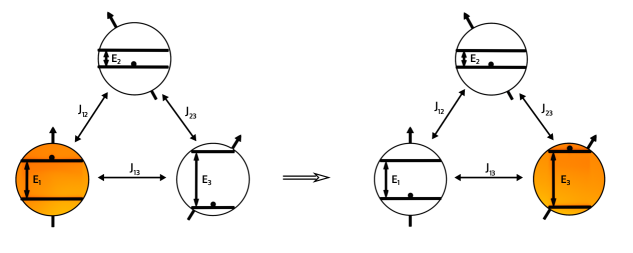
Figure 1: Schematical picture of a three-site (trimer) system. The excitation energy of site $i$ is denoted $E_{i}$ and the coupling between sites $i$ and $j$ is denoted $J_{ij}$. The arrows symbolize the dipole moments in the case where the sites are occupied by localized chromophores. The alignment and distance between these dipole moments determine the inter-site couplings.

The system considered in this study is a network of $N$ localized sites, which are coupled together by their mutual interaction. Each site can be modeled as a two-level quantum system consisting of a ground state $|\mathbf{g}\rangle$ and an excited state $|\mathbf{e}\rangle$. A possible realization could be a molecular aggregate of chromophores, each localized at a site of the network and with $|\mathbf{g}\rangle$ and $|\mathbf{e}\rangle$ being the ground and excited singlet states, respectively. Population of $|\mathbf{e}\rangle$ on site $i$ is denoted $|i\rangle$; hence, $|i\rangle=|\mathbf{g}_{1}\ldots\mathbf{e}_{i}\ldots\mathbf{g}_{N}\rangle$. The inter-site couplings in the case of chromophores are given by the electrostatic dipole-dipole interaction. The coupling strength of a given site pair depends on the alignment of the two dipole moments, as well as their distance to each other. The system in the case of three sites ($N=3$) is illustrated in figure 1.

A tight-binding Hamiltonian can be used to model the time evolution of the system [40]. It reads

$$\hat{H}^{(N)}=\sum_{i}^{N}E_{i}|i\rangle\langle i|+\sum_{i\neq j}^{N}J_{ij}|i\rangle\langle j|,$$ (1)

where $E_{i}$ is the excitation energy of site $|i\rangle$, i.e., the (photon) energy required to excite site $i$ from $\mathbf{g}$ to $\mathbf{e}$, and $J_{ij}$ is the inter-site coupling between $i$ and $j$.

With the help of $\hat{H}^{(N)}$, we wish to transfer an initial excitation localized on site $1$ to site $N$, i.e., $|1\rangle\mapsto e^{-i\hat{H}^{(N)}t}|1\rangle=|N\rangle$ (we put $\hbar=1$ from now on) for some time $t=\tau$. This type of initial condition would in the case of a molecular aggregate correspond to a localized excitation at site $|1\rangle$ prepared by an appropriately tailored laser pulse. We refer to the process as population transfer and we are making the restriction to only one excitation at the time in the network, which reduces the $2^{N}$-dimensional Hilbert space of the system to the $N$-dimensional single-excitation subspace. We also restrict our study to include only real-valued coupling parameters.

3 Quantifying efficiency and coherence

In population transfer there are two natural bases to consider; the site basis, with respect to which the population transfer is described, and the exciton basis, i.e., the Hamiltonian eigenbasis. The delocalization of the evolving quantum state over different sites will be governed by the Hamiltonian parameters and the relation between the coherence in the site and exciton bases is hence of interest. Thus, in this study we focus on these two bases when we are relating efficiency and coherence to each other.

3.1 Quantifying efficiency

Our task is to transfer an initially site-localized state $|\psi(0)\rangle=|1\rangle$ into a site-localized target state $|\psi_{\rm{target}}\rangle=|N\rangle$, by means of the tight-binding Hamiltonian in equation (1). To quantify the efficiency of this process, we use the pure state fidelity [41], which takes the form

$$F=\left|\langle\psi_{\rm{target}}|\hat{U}(t,0)|\psi(0)\rangle\right|=|\langle N|\hat{U}(t,0)|1\rangle|$$ (2)

with $\hat{U}(t,0)=e^{-i\hat{H}^{(N)}t}$. Perfect population transfer corresponds to the case where $F=1$.

3.2 Quantifying coherence

As mentioned in the introduction, the $l_{1}$-norm and the relative entropy of coherence (REOC) satisfy the conditions for being quantifiers of coherence [2]. These two measures have turned out to be the most frequently used when analyzing coherence in different processes (see, e.g., [17, 42]). In this study, we use both $l_{1}$-norm and REOC, in order to cover both geometric and entropic aspects of coherence.

We start by introducing the free pure states as the members of an orthonormal basis $\psi=\{|\psi_{i}\rangle\}$ spanning the Hilbert space of the system. This defines the free states $\hat{\sigma}$ as those that diagonalizes in $\{|\psi_{i}\rangle\}$, i.e., $\hat{\sigma}=\sum_{i}\sigma_{ii}|\psi_{i}\rangle\langle\psi_{i}|$. The idea is to use the concept of free states to quantify the amount of coherence relative $\psi$ in a given density operator $\hat{\rho}$.

Our first measure is the $l_{1}$-norm of coherence, which is induced by the $l_{1}$-matrix norm [43] as follows. Consider the difference $\langle\psi_{i}|\hat{\rho}|\psi_{j}\rangle-\sigma_{ij}\equiv\rho_{ij}^{\psi}-\sigma_{ii}\delta_{ij}$. The corresponding $l_{1}$-matrix norm reads

$$D_{l_{1}}^{\psi}(\hat{\rho},\hat{\sigma})=\sum_{i,j}\left|\rho_{ij}^{\psi}-\sigma_{ii}\delta_{ij}\right|.$$ (3)

The $l_{1}$-norm of coherence $C_{l_{1}}^{\psi}(\hat{\rho})$ of $\hat{\rho}$ with respect to the free basis is given by minimizing $D_{l_{1}}^{\psi}(\hat{\rho},\hat{\sigma})$ over the set of free states. This minimum is obtained for $\hat{\sigma}=\hat{\rho}_{{\rm{diag}}}^{\psi}=\sum_{i}\rho_{ii}^{\psi}|\psi_{i}\rangle\langle\psi_{i}|$, yielding

$$C_{l_{1}}^{\psi}(\hat{\rho})=\sum_{i\neq j}\left|\rho_{ij}^{\psi}\right|=2\sum_{i<j}\left|\rho_{ij}^{\psi}\right|.$$ (4)

Note that the $l_{1}$-norm is bounded by [44]

$$C_{l_{1}}^{\psi}(\hat{\rho})\leq d-1$$ (5)

where $d$ is the dimension of the system. The upper bound is reached for the maximally coherent state (MCS) [45]

$$|{\rm{MCS}}\rangle=\frac{1}{\sqrt{d}}\sum_{i=1}^{d}|\psi_{i}\rangle.$$ (6)

Our second measure is REOC, which is defined by minimizing the relative entropy

$$S(\hat{\rho}\parallel\hat{\sigma})={\rm{Tr}}\left[\hat{\rho}\log_{2}\hat{\rho}\right]-{\rm{Tr}}\left[\hat{\rho}\log_{2}\hat{\sigma}\right]$$ (7)

over the set of free states $\hat{\sigma}$. This minimum can be found by using the identity

$$S(\hat{\rho}\parallel\hat{\sigma})=S(\hat{\rho}_{{\rm{diag}}}^{\psi})-S(\hat{\rho})+S(\hat{\rho}_{{\rm{diag}}}^{\psi}\parallel\hat{\sigma})$$ (8)

with $S(\cdot)$ the von Neumann entropy. Since the lower bound of Klein’s inequality $S(\hat{\rho}_{{\rm{diag}}}^{\psi}\parallel\hat{\sigma})\geq 0$ is obtained if and only if $\hat{\sigma}=\hat{\rho}_{{\rm{diag}}}^{\psi}$, we obtain REOC of $\hat{\rho}$

$$C_{{\rm{REOC}}}^{\psi}(\hat{\rho})=S(\hat{\rho}_{{\rm{diag}}}^{\psi})-S(\hat{\rho}).$$ (9)

For pure states, $S(\hat{\rho})$ vanishes and REOC reduces to

$$C_{{\rm{REOC}}}^{\psi}(\hat{\rho})=S(\hat{\rho}_{{\rm{diag}}}^{\psi}).$$ (10)

REOC is bounded by

$$C_{\rm{REOC}}^{\psi}(\hat{\rho})\leq\log_{2}d$$ (11)

with equality for the maximally coherent state in equation (6).

While $C_{l_{1}}^{\psi}$ and $C_{{\rm{REOC}}}^{\psi}$ are generally time-dependent with respect to the site basis ($\psi=s$) in our system, they are constant in time in the exciton basis ($\psi=e$). The latter can be seen by noting that an initial state $\hat{\rho}(0)=\sum_{i,j}\rho_{ij}^{e}|e_{i}\rangle\langle e_{j}|$, $\{|e_{i}\rangle\}$ being the exciton basis of the time-independent Hamiltonian in equation (1), evolves into $\hat{\rho}(t)=\sum_{i,j}\rho_{ij}^{e}e^{-i\mathcal{E}_{i}t}|e_{i}\rangle\langle e_{j}|e^{i\mathcal{E}_{j}t}$, where $\{\mathcal{E}_{i}\}$ are the exciton energies. Thus, in the exciton basis

$$C_{l_{1}}^{e}(\hat{\rho}(t)) = 2\sum_{i<j}\left|e^{-i\mathcal{E}_{i}t}\rho_{ij}^{e}e^{i\mathcal{E}_{j}t}\right|=2\sum_{i<j}\left|\rho_{ij}^{e}\right|=C_{l_{1}}(\hat{\rho}(0))$$ (12)

for $l_{1}$-norm; the time independence of REOC follows immediately from that $\hat{\rho}_{\rm{diag}}^{e}$ is time-independent.

3.3 Global and local coherence

When $\hat{\rho}$ is representing the full state of the system, $C^{s}(\hat{\rho})$ measures the global coherence of the network of sites. In the $N\geq 3$ case, we can also have local coherence for the subsystem pairs $(i,j)$. These subsystem pairs are described by the reduced states

$$\hat{\rho}_{ij}\doteq\left(\begin{array}[]{cccc}1-(\rho_{ii}^{s}+\rho_{jj}^{s})&0&0&0\\ 0&\rho_{jj}^{s}&\rho_{ij}^{s}&0\\ 0&\rho_{ji}^{s}&\rho_{ii}^{s}&0\\ 0&0&0&0\end{array}\right)$$ (17)

expressed in the product bases $\left\{|\mathbf{g}_{i}\mathbf{g}_{j}\rangle,|\mathbf{g}_{i}\mathbf{e}_{j}\rangle,|\mathbf{e}_{i}\mathbf{g}_{j}\rangle,|\mathbf{e}_{i}\mathbf{e}_{j}\rangle\right\}$.

With respect to the product basis, the local coherence of the pair $(i,j)$ as measured by the $l_{1}$-norm is $C_{l_{1}}^{ij}(\hat{\rho})=2\left|\rho_{ij}^{s}\right|$. This coincides with entanglement as measured by concurrence [46], which is a consequence of the restriction to single-excitation subspace of the full Hilbert space of our $N$-site system. It is hence also possible to relate efficiency to entanglement between sites [47].

3.4 Comparing efficiency and coherence

We wish to develop the quantification of coherence a bit further and specifically, we ask; how much coherence has there been on average in the system during population transfer? We are hence interested in the time-averaged coherence (denoted as TAC in the figures), defined as

$$\overline{C}^{\psi}(t;\hat{\rho})=\frac{1}{t}\int_{0}^{t}C^{\psi}(\hat{\rho}(t^{\prime}))dt^{\prime},$$ (18)

where $C^{\psi}(\hat{\rho}(t))$ is either $C_{l_{1}}^{\psi}(\hat{\rho}(t))$ or $C_{{\rm{REOC}}}^{\psi}(\hat{\rho}(t))$. We refer to $C^{\psi}(\hat{\rho}(t))$ as time-local coherence (denoted as TLC in the figures).

In the following, we optimize $F$, $C^{\psi}$, and $\overline{C}^{\psi}$ numerically and analytically (whenever possible) for a dimer (section 4) and a trimer (section 5) by varying over the parameter space of the tight-binding Hamiltonian in equation (1). The coherence quantities are computed both in the site basis and the exciton basis as well as for both types of coherence measures ($l_{1}$-norm and REOC). We compare the optimal Hamiltonian parameters and time for $F$ to the optimal Hamiltonian parameters and time for $\overline{C}^{\psi}(t;\hat{\rho})$ to see whether they coincide or not, in order to analyze the role of coherence for population transfer.

4 Dimer case

We first consider population transfer from site $1$ to site $2$ in a dimer ($N=2$). This process can be understood as tunneling through an energy barrier defined by the difference in site energies, and driven by the inter-site coupling. In this sense, the dimer enables us to examine efficiency and coherence associated with the tunneling mechanism alone.

The tight-binding dimer Hamiltonian takes the form

$$\hat{H}^{(2)}=\omega\big{[}\cos\theta(|1\rangle\langle 1|-|2\rangle\langle 2|)+\sin\theta(|1\rangle\langle 2|+|2\rangle\langle 1|)\big{]},$$ (19)

where $\omega=\sqrt{E^{2}+J_{12}^{2}}$ and $\tan\theta=J_{12}/E$, $E$ being related to the site excitation energies as $E=\left(E_{1}-E_{2}\right)/2$. The time evolution

$$|1\rangle\mapsto\hat{U}(t,0)|1\rangle = \big{(}\cos\omega t-i\cos\theta\sin\omega t\big{)}|1\rangle-i\sin\theta\sin\omega t|2\rangle$$ (20)

is characterized by the single frequency $\omega$. Note that the energy gap of the two exciton states is $2\omega$. Without loss of generality, we assume $E,J_{12}\geq 0$ and $0\leq\theta\leq\frac{\pi}{2}$ (thus, $\sin\theta\geq 0$ and $\cos\theta\geq 0$) in the following.

The optimization of time-averaged coherence is performed numerically. The Hamiltonian parameters and time are varied over $-0.500\leq E_{i}\leq 0.500$, $-0.500\leq J_{12}\leq 0.500$ and $0\leq t\leq 10$ in steps of $\Delta E_{i}=0.01,\Delta J_{12}=0.01$, and $\Delta t=0.001$, respectively. We limit the study to maximum occurring in the given time interval - there might be Hamiltonian parameter sets for which maximum are obtained at $t>10$.

4.1 Population transfer efficiency

The fidelity is given by

$$F(\theta,t)=\big{|}\langle 2|\hat{U}(t,0)|1\rangle\big{|}=\sin\theta\left|\sin\omega t\right|,$$ (21)

which is a periodic function in time with period (revival time) $T=\pi/\omega$. The fidelity reaches its maximum

$$F_{\max}(\theta)=\max_{t}F(\theta,t)=\sin\theta$$ (22)

at $t=\pi/(2\omega)=\tau$, being half the revival time. Thus, the speed of the transfer process is inversely proportional to the energy gap $2\omega$. Perfect population transfer, i.e., $F=1$, occurs for $\theta=\pi/2$, which holds whenever $E=0$ and $J_{12}\neq 0$.

4.2 Coherence

The $l_{1}$-norm and REOC are directly related for pure dimer states $\hat{\rho}=|\phi\rangle\langle\phi|$. To see this, we express $|\phi\rangle$ in terms of an arbitrary free basis $\psi=\{|\psi_{1}\rangle,|\psi_{2}\rangle\}$ as $|\phi\rangle=c_{1}|\psi_{1}\rangle+c_{2}|\psi_{2}\rangle$, yielding

$$C_{l_{1}}^{\psi}(\hat{\rho})=2\left|c_{1}c_{2}\right|=2\left|c_{2}\right|\sqrt{1-\left|c_{2}\right|^{2}}$$ (23)

and

$$C_{\rm{REOC}}^{\psi}(\hat{\rho})=-\left|c_{1}\right|^{2}\log_{2}\left|c_{1}\right|^{2}-\left|c_{2}\right|^{2}\log_{2}\left|c_{2}\right|^{2}=h\left(\left|c_{2}\right|^{2}\right),$$ (24)

where $h(x)=-(1-x)\log_{2}(1-x)-x\log_{2}x$ is the binary Shannon entropy and we have used that $\left|c_{1}\right|^{2}+\left|c_{2}\right|^{2}=1$. By inverting equation (23) and inserting into equation (24), we find

$$C_{\rm{REOC}}^{\psi}(\hat{\rho})=h\left(\frac{1+\sqrt{1-\left[C_{l_{1}}^{\psi}(\hat{\rho})\right]^{2}}}{2}\right),$$ (25)

which establishes a general relation between the two coherence measures in the dimer case. We further note that $C^{\psi}\leq 1$ with equality for $|\phi\rangle=|\rm{MCS}\rangle=\frac{1}{\sqrt{2}}\left(|\psi_{1}\rangle+|\psi_{2}\rangle\right)$.

4.3 Comparing population transfer efficiency and coherence

Site basis

The time-local $l_{1}$-norm and REOC in the site basis are given by

$$C_{l_{1}}^{s}(\theta,t) = 2\sqrt{1-\sin^{2}\theta\sin^{2}\omega t}\sin\theta|\sin\omega t|$$ (26)

$$= 2F(\theta,t)\sqrt{1-\left[F(\theta,t)\right]^{2}}$$

and

$$C_{{\rm{REOC}}}^{s}(\theta,t) = h(\sin^{2}\theta\sin^{2}\omega t)=h\left(\left[F(\theta,t)\right]^{2}\right),$$ (27)

where we have used the expression for the fidelity in equation (21). We see that $C_{l_{1}}^{s}(\theta,t)$ and $C_{{\rm{REOC}}}^{s}(\theta,t)$ take their maximal value at $F(\theta,t)=\sin\theta$ for $\sin\theta\leq\frac{1}{\sqrt{2}}$ and at $F(\theta,t)=\frac{1}{\sqrt{2}}$ for $\sin\theta\geq\frac{1}{\sqrt{2}}$, where the former occurs at the time of maximal population transfer $t=\pi/(2\omega)$ and the latter at

$$t=\frac{1}{\omega}\arcsin\left[\frac{1}{\sqrt{2}\sin\theta}\right].$$ (28)

Explicitly, these maximal coherence values are

$$\max_{t}C_{l_{1}}^{s}(\theta,t) = \left\{\begin{array}[]{cc}\sin 2\theta,&0\leq\theta\leq\frac{\pi}{4},\\ 1,&\frac{\pi}{4}\leq\theta\leq\frac{\pi}{2},\end{array}\right.$$ (31)

$$\max_{t}C_{\rm{REOC}}^{s}(\theta,t) = \left\{\begin{array}[]{cc}h\left(\sin^{2}\theta\right),&0\leq\theta\leq\frac{\pi}{4},\\ 1,&\frac{\pi}{4}\leq\theta\leq\frac{\pi}{2}.\end{array}\right.$$ (34)

We note that while maximal efficiency and maximal coherence occur simultaneously for $0\leq\theta\leq\frac{\pi}{4}$, maximal coherence precedes maximal population transfer for $\frac{\pi}{4}<\theta\leq\frac{\pi}{2}$, as is evident from equation (28). Furthermore, when the efficiency increases, an increasingly larger part of the coherence is localized in time before the transfer has been completed. This indicates that time-local coherence plays a role for the population transfer in the dimer system.

. .

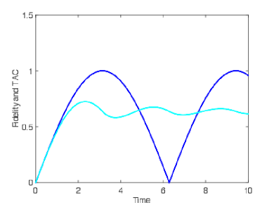
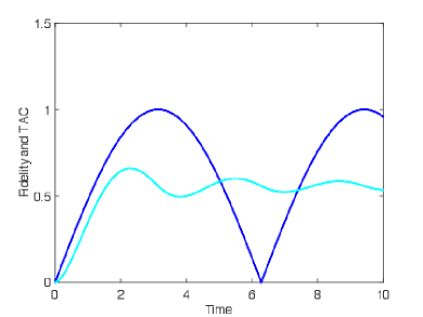
Figure 2: Efficiency and time-averaged coherence for a Hamiltonian that optimizes $F(\theta,\tau)$ in a dimer. The left panel shows $F(\theta,t)$ (blue) and $\overline{C}_{l_{1}}^{s}(\theta,t)$ (cyan). The right panel shows $F(\theta,t)$ (blue) and $\overline{C}_{\rm{REOC}}^{s}(\theta,t)$ (cyan).

. .

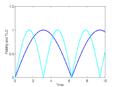
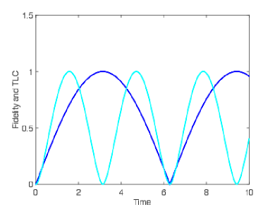
Figure 3: Efficiency and time-local coherence for a Hamiltonian that optimizes $F(\theta,\tau)$ in a dimer. The left panel shows $F(\theta,t)$ (blue) and $C_{l_{1}}^{s}(\theta,t)$ (cyan). The right panel shows $F(\theta,t)$ (blue) and $C_{\rm{REOC}}^{s}(\theta,t)$ (cyan).

The relationship between $F(\theta,t)$ and $\overline{C}^{s}(\theta,t)$ and between $F(\theta,t)$ and $C^{s}(\theta,t)$ for perfect population transfer $\theta=\pi/2$, i.e., $E=0$, can be seen in figures 2 and 3, respectively. The results are shown for $J_{12}=\frac{1}{2}$ for which $\tau=\pi$. A closer inspection reveals that $\overline{C}^{s}(\theta,t)$ in figure 2 oscillates roughly around the time-averaged coherence $\overline{C}^{s}(\theta,\tau)$. The amplitude of these oscillations decreases, suggesting the existence of a long-time asymptotic value, as will be discussed in detail in section 6 below. The time-local coherence in figure 3 maximize at precisely half the transfer time, in accordance with equation (28); on the other hand, they vanish when the perfect transfer is completed. In terms of correlation between the two sites, efficiency is improved when entanglement is built up in a symmetric fashion to its maximum at exactly half the population transfer time and then drops to zero when the population returns to site $1$.

The relationship between $F(\theta,t)$ and $\overline{C}^{s}(\theta,t)$ and between $F(\theta,t)$ and $C^{s}(\theta,t)$ for parameters optimizing the time-averaged coherence $\overline{C}^{s}(\theta,t)$, can be seen in figures 4 ($l_{1}$-norm) and 5 (REOC). The Hamiltonian parameters, shown in table 1, differ slightly whether the optimization is for time-averaged $l_{1}$-norm or REOC. As can be seen, perfect population transfer can never occur for these parameter sets, i.e., maximal time-averaged coherence does not imply maximal efficiency in the population transfer. We further note that $F(\theta,t)$ and $\overline{C}^{s}(\theta,t)$ do not maximize simultaneously and that $C^{s}(\theta,t)$ is nonzero at maximal transfer for these two parameter sets. Thus, the efficiency and time-averaged coherence order the Hamiltonians differently with respect to their ability to transfer population between sites.

. .

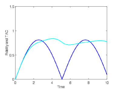
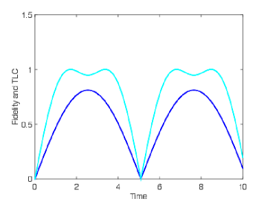
Figure 4: Efficiency and coherence for a Hamiltonian that optimizes $\overline{C}_{l_{1}}^{s}(\theta,t)$ in a dimer. The left panel shows $F(\theta,t)$ (blue) and $\overline{C}_{l_{1}}^{s}(\theta,t)$ (cyan). The right panel shows $F(\theta,t)$ (blue) and $C_{l_{1}}^{s}(\theta,t)$ (cyan).

. .

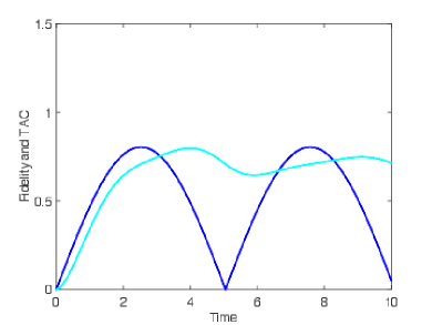
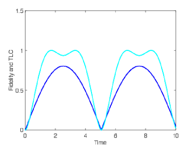
Figure 5: Efficiency and coherence for a Hamiltonian that optimizes $\overline{C}_{\rm{REOC}}^{s}(\theta,t)$ in a dimer. The left panel shows $F(\theta,t)$ (blue) and $\overline{C}_{\rm{REOC}}^{s}(\theta,t)$ (cyan). The right panel shows $F(\theta,t)$ (blue) and $C_{\rm{REOC}}^{s}(\theta,t)$ (cyan).

	$E$	$J_{12}$
$l_{1}$-norm	0.36	0.50
REOC	0.37	0.50

Table 1: Hamiltonian parameters optimizing $\overline{C}^{s}$ in a dimer. These parameter values correspond to $F_{\max}(\theta)\approx 0.81$ and $0.80$ for optimal $l_{1}$-norm and REOC, respectively.

Exciton basis

The exciton states read

$$|e_{+}\rangle = \cos\frac{\theta}{2}|1\rangle+\sin\frac{\theta}{2}|2\rangle,$$

$$|e_{-}\rangle = -\sin\frac{\theta}{2}|1\rangle+\cos\frac{\theta}{2}|2\rangle$$ (35)

with exciton energies $\mathcal{E}_{\pm}=\pm\omega$. We find the $l_{1}$-norm measure of coherence and REOC to be

$$C_{l_{1}}^{e}(\theta)=\sin\theta=F_{\max}(\theta)$$ (36)

and

$$C_{{\rm{REOC}}}^{e}(\theta)=h\left(\frac{1+\sqrt{1-\sin^{2}\theta}}{2}\right)=h\left(\frac{1+\sqrt{1-\left[F_{\max}(\theta)\right]^{2}}}{2}\right),$$ (37)

respectively, where we have used the expression for the fidelity maximum in equation (22). Since coherence is time-independent in the exciton basis, there is apparently no distinction between the time-local and time-averaged coherence in this basis.

The key observation is that $C_{l_{1}}^{e}(\theta)$ and $C_{{\rm{REOC}}}^{e}(\theta)$ are strictly monotonically increasing functions of the fidelity maximum. This implies that coherence with respect to the exciton basis increases with the population transfer efficiency and becomes maximal for perfect population transfer. Thus, population transfer efficiency is in one-to-one correspondence with coherence in the exciton basis in the case of a dimer system.

5 Trimer case

We next present our results for the case of population transfer from site $1$ to site $3$ in a trimer. This process can take place via two distinct pathways, either $1\rightarrow 3$ directly or $1\rightarrow 2\rightarrow 3$. In this sense, the trimer is the smallest system that can capture constructive and destructive interference between different pathways in a site network.

The tight-binding trimer Hamiltonian reads

$$\hat{H}^{(3)} = E_{1}|1\rangle\langle 1|+E_{2}|2\rangle\langle 2|+E_{3}|3\rangle\langle 3|$$ (38)

$$+(J_{12}|1\rangle\langle 2|+J_{23}|2\rangle\langle 3|+J_{13}|1\rangle\langle 3|+{\rm{h.c.}}).$$

Optimization of population transfer efficiency and time-averaged coherence is performed numerically. The Hamiltonian parameters and time are varied over $-0.500\leq E_{i}\leq 0.500$, $-0.500\leq J_{ij}\leq 0.500$ and $0\leq t\leq 10$ in steps of $\Delta E_{i}=0.1,\Delta J_{ij}=0.1$, and $\Delta t=0.01$, respectively. The larger step size in the trimer compared to the dimer is due to computational limitations.

It turns out again that optimal efficiency in the population transfer is not obtained for parameter values that optimize the time-averaged coherence. In the trimer, unlike in the dimer, the sign of the relative site energies and inter-site couplings matters; two parameter sets only differing in the signs of these parameters have (in general) different maxima for fidelity and time-averaged coherence. By using the bounds in equations (5) and (11), we find

$$C_{l_{1}}^{\psi}(\hat{\rho})\leq 2$$ (39)

and

$$C_{\rm{REOC}}^{\psi}(\hat{\rho})\leq\log_{2}3\approx 1.59$$ (40)

with equality for the maximally coherent state $|\rm{MCS}\rangle=\frac{1}{\sqrt{3}}\sum_{i=1}^{3}|\psi_{i}\rangle$.

5.1 Efficiency and coherence for perfect population transfer

To put the Hamiltonian on convenient form, we note that the local energy term $\sum_{i=1}^{3}E_{i}|i\rangle\langle i|$ in equation (38) can be rewritten as

$$\sum_{i=1}^{3}E_{i}|i\rangle\langle i| \sim \frac{E_{1}-E_{3}}{2}\Big{(}|1\rangle\langle 1|-|3\rangle\langle 3|\Big{)}+\left(E_{2}-\frac{E_{1}+E_{3}}{2}\right)|2\rangle\langle 2|$$ (41)

$$= E_{13}\Big{(}|1\rangle\langle 1|-|3\rangle\langle 3|\Big{)}+\widetilde{E}|2\rangle\langle 2|,$$

where we have ignored a trivial zero-point energy term and defined $E_{13}=(E_{1}-E_{3})/2$ and $\widetilde{E}=E_{2}-(E_{1}+E_{3})/2$. The results from the numerical calculations show that a necessary, but not sufficient condition for perfect population transfer between sites $1$ and $3$ is $E_{13}=0$ and $\left|J_{12}\right|=\left|J_{23}\right|$, the latter being consistent with Lemma 2 of [37] for an open spin chain. By combining these observations and equation (41), we may put $J_{12}=\sigma J_{23}$ with the ‘parity’ $\sigma=\pm 1$ in terms of which the trimer Hamiltonian takes the form

$$\hat{H}^{(3)} = \widetilde{E}|2\rangle\langle 2|+J_{23}\Big{(}|1\rangle\langle 2|+|2\rangle\langle 1|\Big{)}$$ (42)

$$+\sigma J_{23}\Big{(}|2\rangle\langle 3|+|3\rangle\langle 2|\Big{)}+J_{13}\Big{(}|1\rangle\langle 3|+|3\rangle\langle 1|\Big{)}$$

when it allows for perfect population transfer. Here, $J_{12}=\sigma J_{23}$ with the ‘parity’ $\sigma=\pm 1$. By inspection, we find an exciton state

$$|e_{d}\rangle=\frac{1}{\sqrt{2}}\big{(}|1\rangle-\sigma|3\rangle\big{)}$$ (43)

with corresponding exciton energy $\mathcal{E}_{d}=-\sigma J_{13}$. Note that $|e_{d}\rangle$ is a ‘dark’ eigenstate in the sense that it does not contain the state $|2\rangle$. In order to find the remaining two exciton states and energies, we eliminate $|e_{d}\rangle$ and find the $2\times 2$ block

$$H_{2\times 2}^{(3)}=\widetilde{E}|2\rangle\langle 2|+\sigma J_{13}|b\rangle\langle b|+\sqrt{2}J_{23}\Big{(}|2\rangle\langle b|+|b\rangle\langle 2|\Big{)}$$ (44)

with $|b\rangle=\frac{1}{\sqrt{2}}\big{(}|1\rangle+\sigma|3\rangle\big{)}$. This can be diagonalized by standard methods, yielding the exciton energies

$$\mathcal{E}_{\pm}=\frac{\widetilde{E}+\sigma J_{13}}{2}\pm\frac{1}{2}\sqrt{(\widetilde{E}-\sigma J_{13})^{2}+8J_{23}^{2}}$$ (45)

and corresponding exciton states

$$|e_{+}\rangle = \cos\frac{\vartheta}{2}|2\rangle+\sin\frac{\vartheta}{2}|b\rangle,$$

$$|e_{-}\rangle = -\sin\frac{\vartheta}{2}|2\rangle+\cos\frac{\vartheta}{2}|b\rangle,$$ (46)

where

$$\tan\vartheta=\frac{2\sqrt{2}J_{23}}{\widetilde{E}-\sigma J_{13}}.$$ (47)

We note that the exciton states and energies depend nontrivially on the parity $\sigma$. Thus, the two parity cases must be treated separately in the following analysis.

The time evolution operator associated with the Hamiltonian in equation (42) takes the form

$$\hat{U}(t,0) = e^{-i\mathcal{E}_{d}t}|e_{d}\rangle\langle e_{d}|+e^{-i\mathcal{E}_{+}t}|e_{+}\rangle\langle e_{+}|$$ (48)

$$+e^{-i\mathcal{E}_{-}t}|e_{-}\rangle\langle e_{-}|.$$

We find the fidelity of the population transfer $1\rightarrow 3$:

$$F(\vec{h},t) = |\langle 3|\hat{U}(t,0)|1\rangle|$$ (49)

$$= \frac{1}{2}\left|1-e^{-i\left(\mathcal{E}_{+}-\mathcal{E}_{d}\right)t}\sin^{2}\frac{\vartheta}{2}-e^{-i\left(\mathcal{E}_{-}-\mathcal{E}_{d}\right)t}\cos^{2}\frac{\vartheta}{2}\right|$$

$$= \frac{1}{2}\left|1-e^{-i\omega_{+}t}\sin^{2}\frac{\vartheta}{2}-e^{-i\omega_{-}t}\cos^{2}\frac{\vartheta}{2}\right|,$$

where $\vec{h}$ denote the set of relevant Hamiltonian parameters and we have identified two fundamental frequencies

$$\omega_{\pm} = \mathcal{E}_{\pm}-\mathcal{E}_{d}=\frac{\widetilde{E}+3\sigma J_{13}}{2}\pm\frac{1}{2}\sqrt{(\widetilde{E}-\sigma J_{13})^{2}+8J_{23}^{2}}.$$ (50)

Perfect population transfer occurs provided there exists a ‘perfect transfer time’ $\tau$ satisfying

$$\omega_{\pm}\tau=(2n_{\pm}+1)\pi,$$ (51)

where $n_{\pm}$ are arbitrary integers. We thus end up with the following necessary and sufficient condition: perfect population transfer occurs if and only if there exist integers $n_{\pm}$ such that

$$\frac{\omega_{+}}{\omega_{-}}=\frac{2n_{+}+1}{2n_{-}+1}.$$ (52)

Let us consider the two special cases $\omega_{+}=\pm\omega_{-}$. By using equation (50), we see that the $\omega_{+}=\omega_{-}$ case corresponds $\widetilde{E}=\sigma J_{13}$ and $J_{23}=0$. Here, the Hamiltonian takes the form

$$\hat{H}^{(3)}=J_{13}\Big{(}\sigma|2\rangle\langle 2|+|1\rangle\langle 3|+|3\rangle\langle 1|\Big{)}$$ (53)

and the smallest positive perfect transfer time is

$$\tau=\frac{\pi}{2|J_{13}|}.$$ (54)

Similarly, the $\omega_{+}=-\omega_{-}$ case corresponds $\widetilde{E}+3\sigma J_{13}=0$ and $J_{23}$ arbitrary. The corresponding Hamiltonian reads

$$\hat{H}^{(3)} = -3\sigma J_{13}|2\rangle\langle 2|+J_{23}\Big{(}|1\rangle\langle 2|+|2\rangle\langle 1|\Big{)}$$ (55)

$$+\sigma J_{23}\Big{(}|2\rangle\langle 3|+|3\rangle\langle 2|\Big{)}+J_{13}\Big{(}|1\rangle\langle 3|+|3\rangle\langle 1|\Big{)},$$

which contains for $J_{13}=0$ a resonant $\Lambda$ system [48] with real-valued and equal inter-site couplings. The smallest positive transfer time now reads

$$\tau=\frac{\pi}{\sqrt{4J_{13}^{2}+2J_{23}^{2}}}.$$ (56)

Coherence in the site basis

The $l_{1}$-norm in the site basis is determined by the off-diagonal elements

$$\left|\rho_{ij}^{s}(t)\right| = \left|\langle i|\hat{U}(t,0)|1\rangle\langle 1|U^{\dagger}(t,0)|j\rangle\right|$$ (57)

$$\equiv f_{i}(t)f_{j}(t),$$

where $f_{i}(t)=\left|\langle i|\hat{U}(t,0)|1\rangle\right|$ and we have used that $\langle 1|U^{\dagger}(t,0)|j\rangle=\langle j|\hat{U}(t,0)|1\rangle^{\ast}$. Physically, $[f_{1}(t)]^{2}$ is the survival probability of the initial state; $f_{2}(t)$ ($f_{3}(t)$) is the fidelity of the $1\rightarrow 2$ ($1\rightarrow 3$) population transfer. We find the $l_{1}$-norm

$$C_{l_{1}}^{s}(\vec{h},t)=2\big{[}f_{1}(t)f_{2}(t)+f_{1}(t)f_{3}(t)+f_{2}(t)f_{3}(t)\big{]}.$$ (58)

Similarly, REOC is determined by the incoherent density operator

$$\hat{\rho}_{\rm{diag}}^{s}(t)=\sum_{i=1}^{3}\left[f_{i}(t)\right]^{2}|i\rangle\langle i|.$$ (59)

Explictly,

$$C_{\rm{REOC}}^{s}(\vec{h},t)=-\sum_{i=1}^{2}\left[f_{i}(t)\right]^{2}\log_{2}\left[f_{i}(t)\right]^{2}.$$ (60)

We see that the $l_{1}$-norm and REOC in the trimer are determined by the same three functions $f_{1}(t),f_{2}(t)$, and $f_{3}(t)$.

For $E_{13}=0$ and $|J_{12}|=|J_{23}|$ we have that $f_{3}(t)=F(\vec{h},t)$ given by equation (49). The remaining two functions read

$$f_{1}(t) = \frac{1}{2}\left|1+e^{-i\omega_{+}t}\sin^{2}\frac{\vartheta}{2}+e^{-i\omega_{-}t}\cos^{2}\frac{\vartheta}{2}\right|,$$

$$f_{2}(t) = \frac{1}{\sqrt{2}}\left|\sin\vartheta\sin\left[\frac{\left(\omega_{+}-\omega_{-}\right)t}{2}\right]\right|.$$ (61)

Exciton basis

Since the coherence in the exciton basis are time-independent, all information is contained in the initial state $|1\rangle$ expressed in terms of the exciton states. Explicitly, we find

$$|1\rangle=\frac{1}{\sqrt{2}}\left(|e_{d}\rangle+\sin\frac{\vartheta}{2}|e_{+}\rangle+\cos\frac{\vartheta}{2}|e_{-}\rangle\right).$$ (62)

The $l_{1}$-norm is given by the off-diagonal elements, which read

$$\left|\rho_{d+}^{e}\right| = \frac{1}{2}r,$$

$$\left|\rho_{+-}^{e}\right| = \frac{1}{2}\sqrt{1-r^{2}},$$

$$\left|\rho_{d-}^{e}\right| = \frac{1}{2}r\sqrt{1-r^{2}},$$ (63)

where we have defined $r=\left|\sin(\vartheta/2)\right|$. We obtain the $l_{1}$-norm

$$C_{l_{1}}^{e}=r+\sqrt{1-r^{2}}+r\sqrt{1-r^{2}}\leq\frac{1}{2}+\sqrt{2}\approx 1.9142$$ (64)

with equality for $r=\frac{1}{\sqrt{2}}$. This is slightly less than the $l_{1}$-norm of the maximally coherent state.

REOC is determined by the diagonal elements of $|1\rangle\langle 1|$ in the exciton basis, which are

$$\rho_{dd}^{e} = \frac{1}{2},$$

$$\rho_{++}^{e} = \frac{r^{2}}{2},$$

$$\rho_{--}^{e} = \frac{1-r^{2}}{2}.$$ (65)

We obtain

$$C_{{\rm{REOC}}}^{e} = -\frac{1}{2}\log_{2}\frac{1}{2}-\frac{r^{2}}{2}\log_{2}\frac{r^{2}}{2}$$ (66)

$$-\frac{1-r^{2}}{2}\log_{2}\frac{1-r^{2}}{2}$$

$$= 1-\frac{r^{2}}{2}\log_{2}r^{2}-\frac{1-r^{2}}{2}\log_{2}(1-r^{2})$$

$$= 1+\frac{1}{2}h\left(r^{2}\right)\leq\frac{3}{2}$$

with equality again for $r=\frac{1}{\sqrt{2}}$.

The maximal value is slightly less than that of the maximally coherent trimer state in the exciton basis. The condition $r=\frac{1}{\sqrt{2}}$ can be expressed in terms of the original Hamiltonian parameters as

$$\widetilde{E}-\sigma J_{13}=0,\ J_{23}\neq 0.$$ (67)

Thus, given the restriction to perfect population transfer, the coherence in the exciton basis can take their maximal value even for nonzero energy barrier, due to constructive interference between the two pathways opened up by the nonzero couplings between the three sites. This should be compared with the dimer case, where maximal coherence in the exciton basis occurs only when the energy barrier vanishes.

5.2 Efficiency and coherence for optimized coherence

Site basis

In the trimer case, the Hamiltonian parameter values that optimize $\overline{C}^{s}(\vec{h},t)$ are roughly the same for $l_{1}$-norm and REOC. When only the absolute value (not the sign) of the parameters are considered, there are two sets of parameters. They are shown in tables 2 and 3. Note that $E_{13}\neq 0$ for both sets, which means that perfect population transfer cannot occur for these parameter values.

$E_{1}-E_{3}$	$E_{2}-E_{3}$	$J_{12}$	$J_{23}$	$J_{13}$
$0.2$	$-0.8$	$-0.5$	$-0.1$	$-0.5$
$0.2$	$-0.8$	$0.5$	$0.1$	$-0.5$
$0.2$	$-0.8$	$0.5$	$-0.1$	$0.5$
$0.2$	$-0.8$	-$0.5$	$0.1$	$0.5$

Table 2: Set 1 of Hamiltonian parameters (value and sign) for optimizing $\overline{C}^{s}(\vec{h},t)$ in a trimer. Note that the remaining eight sign combinations do not optimize $\overline{C}^{s}(\vec{h},t)$.

$E_{1}-E_{3}$	$E_{2}-E_{3}$	$J_{12}$	$J_{23}$	$J_{13}$
$1.0$	$0.8$	$-0.5$	$-0.1$	$-0.5$
$1.0$	$0.8$	$0.5$	$0.1$	$-0.5$
$1.0$	$0.8$	$0.5$	$-0.1$	$0.5$
$1.0$	$0.8$	$-0.5$	$0.1$	$0.5$

Table 3: Set 2 of Hamiltonian parameters (value and sign) for the two sets optimizing $\overline{C}^{s}(\vec{h},t)$ in a trimer. Note that the remaining eight sign combinations do not optimize $\overline{C}^{s}(\vec{h},t)$.

	Set $1$	Set $2$
$\overline{C}_{l_{1}}^{12}$	$0.54$	$0.66$
$\overline{C}_{l_{1}}^{23}$	$0.56$	$0.56$
$\overline{C}_{l_{1}}^{13}$	$0.66$	$0.54$

Table 4: Local coherence $\overline{C}_{l_{1}}^{12}(\vec{h},t)$ , $\overline{C}_{l_{1}}^{23}(\vec{h},t)$ and $\overline{C}_{l_{1}}^{13}(\vec{h},t)$ for the two sets of parameters optimizing $\overline{C}^{s}(\vec{h},t)$ in a trimer.

. .

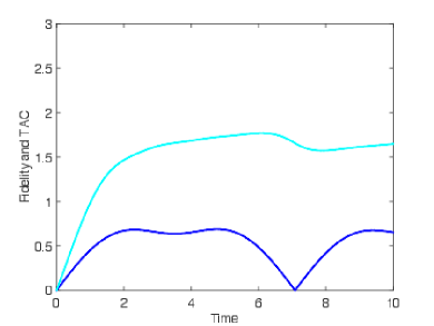
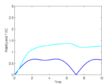
Figure 6: Efficiency and time-averaged coherence for a Hamiltonian that optimizes $\overline{C}^{s}(\vec{h},t)$ in a trimer. The left panel shows $F(\vec{h},t)$ (blue) and $\overline{C}_{l_{1}}^{s}(\vec{h},t)$ (cyan). The right panel shows $F(\vec{h},t)$ (blue) and $\overline{C}_{\rm{REOC}}^{s}(\vec{h},t)$ (cyan).

. .

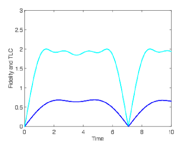
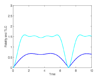
Figure 7: Efficiency and time-local coherence for a Hamiltonian that optimizes $\overline{C}^{s}(\vec{h},t)$ in a trimer. The left panel shows $F(\vec{h},t)$ (blue) and $C_{l_{1}}^{s}(\vec{h},t)$ (cyan). The right panel shows $F(\vec{h},t)$ (blue) and $C_{\rm{REOC}}^{s}(\vec{h},t)$ (cyan).

. .

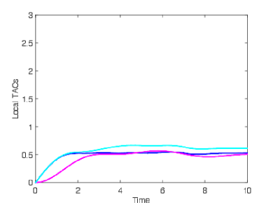
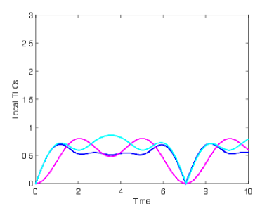
Figure 8: Local coherences for a Hamiltonian that optimizes $\overline{C}^{s}(\vec{h},t)$ in a trimer. The left panel shows $\overline{C}_{l_{1}}^{12}(\vec{h},t)$ (blue), $\overline{C}_{l_{1}}^{23}(\vec{h},t)$ (magneta) and $\overline{C}_{l_{1}}^{13}(\vec{h},t)$ (cyan). The right panel shows $C_{l_{1}}^{12}(\vec{h},t)$ (blue), $C_{l_{1}}^{23}(\vec{h},t)$ (magneta) and $C_{l_{1}}^{13}(\vec{h},t)$ (cyan).

The two sets of parameters optimizing $\overline{C}^{s}(\vec{h},t)$ differ from each other. All of them have the same maximal value for $\overline{C}^{s}(\vec{h},t)$ and $C^{s}(\vec{h},t)$, but $F_{\max}$ is higher in set 1 ($F_{\max}=0.69$) than in set 2 ($F_{\max}=0.60$). Also, the maximal local time-averaged coherence differs between the two sets, see table 4. As can be seen, $\overline{C}_{l_{1}}^{12}(\vec{h},t)$ and $\overline{C}_{l_{1}}^{13}(\vec{h},t)$ are interchanged between the two sets.

In figures 6 and 7, $\overline{C}^{s}(\vec{h},t)$ and $C^{s}(\vec{h},t)$, respectively, and $F(\vec{h},t)$ for the Hamiltonian parameters in set 1 can be seen. Note that all parameter settings in the set give the same time-dependence. Again, maximum of $\overline{C}^{s}(\vec{h},t)$ and maximum of $F(\vec{h},t)$ do not coincide in time, but $C^{s}(\vec{h},t)$ and $F(\vec{h},t)$ are zero simultaneously. Note that the upper bounds $C_{l_{1}}^{s}=2$ and $C_{{\rm{REOC}}}^{s}=\log_{2}3\approx 1.58$ are reached in this parameter set.

Local coherence as a function of time for the $l_{1}$-norm (which coincides with concurrence) are shown in figure 8. It can be seen that even though for this set, $\overline{C}_{l_{1}}^{13}(\vec{h},t)$ reaches a larger value than $\overline{C}_{l_{1}}^{12}(\vec{h},t)$ and $\overline{C}_{l_{1}}^{23}(\vec{h},t)$, $C_{l_{1}}^{13}(\vec{h},t)$ and $C_{l_{1}}^{12}(\vec{h},t)$ have local minima at the time for maximum of $F(\vec{h},t)$ while $C_{l_{1}}^{23}(\vec{h},t)$ has a maximum. Table 4 also reveals that $\overline{C}_{l_{1}}^{23}(\vec{h},t)$ has the same maximal value in both parameter sets.

Exciton basis

Optimization of $\overline{C}^{e}(\vec{h})$ yields infinitely many Hamiltonian parameter sets, but none of them coincides with the parameter sets of optimal $F(\vec{h},\tau)$ or optimal $\overline{C}^{s}(\vec{h},t)$. Whether there exists a basis where the $l_{1}$-norm coincides with fidelity, as in the dimer case, remains an open question.

6 Long-term behavior of time-averaged coherence

In section 4, it can be seen in the figures that the time-averaged coherence in the site basis seem to converge to a specific limit over long times. In this section we discuss this behaviour and extend the time frame of calculations of time-averaged coherence.

The evolution of the dimer state is $\pi/\omega$-periodic in $t$ and time-inversion symmetric within each period. It thus follows that

$$\int_{0}^{n\frac{\pi}{\omega}}C^{s}(\hat{\rho}(t^{\prime}))dt^{\prime}=2n\int_{0}^{\frac{\pi}{2\omega}}C^{s}(\hat{\rho}(t^{\prime}))dt^{\prime},$$ (68)

which implies

$$\overline{C}^{s}\left(n\frac{\pi}{\omega}+\delta t;\hat{\rho}\right)=\frac{1}{n\frac{\pi}{\omega}+\delta t}\int_{0}^{n\frac{\pi}{\omega}+\delta t}C^{s}(\hat{\rho}(t^{\prime}))dt^{\prime}$$

$$=\frac{1}{n\frac{\pi}{\omega}+\delta t}\left(2n\int_{0}^{\frac{\pi}{2\omega}}C^{s}(\hat{\rho}(t^{\prime}))dt^{\prime}+\int_{0}^{\delta t}C^{s}(\hat{\rho}(t^{\prime}))dt^{\prime}\right).$$ (69)

By assuming $0\leq\delta t\leq\frac{\pi}{\omega}$, we find

$$\lim_{n\rightarrow\infty}\overline{C}^{s}\left(n\frac{\pi}{\omega}+\delta t;\hat{\rho}\right)=\frac{2\omega}{\pi}\int_{0}^{\frac{\pi}{2\omega}}C^{s}(\hat{\rho}(t^{\prime}))dt^{\prime}=\overline{C}^{s}\left(\tau;\hat{\rho}\right),$$ (70)

which entails that the long-term behavior is determined by the time-averaged coherence over one transfer period. It is therefore sufficient to examine the time-averaged $l_{1}$-norm and REOC at $t=\pi/(2\omega)=\tau$.

The time-averaged $l_{1}$-norm measure of coherence over one transfer period in the site basis reads

$$\overline{C}_{l_{1}}^{s}(t;\hat{\rho})\equiv\overline{C}_{l_{1}}^{s}(\theta,t)=\frac{2}{t}\int_{0}^{t}\sqrt{\cos^{2}\theta+\sin^{2}\theta\cos^{2}\omega t^{\prime}}\sin\theta|\sin\omega t^{\prime}|dt^{\prime}.$$ (71)

We evaluate $\overline{C}_{l_{1}}^{s}(\theta,t)$ at $t=\pi/(2\omega)=\tau$ by making the variable substitution $t^{\prime}\mapsto x=\sin\theta\cos\omega t^{\prime}$, yielding

$$\overline{C}_{l_{1}}^{s}\left(\theta,\tau\right)=\frac{4}{\pi}\int_{0}^{\sin\theta}\sqrt{\cos^{2}\theta+x^{2}}dx$$

$$=\frac{2}{\pi}\left[\sin\theta+\cos^{2}\theta\ln\left(\frac{1+\sin\theta}{\cos\theta}\right)\right]$$

$$=\frac{2}{\pi}\left[F_{\max}(\theta)+\left(1-\left[F_{\max}(\theta)\right]^{2}\right)\ln\left(\frac{1+F_{\max}(\theta)}{\sqrt{1-\left[F_{\max}(\theta)\right]^{2}}}\right)\right].$$

We thus find

$$\overline{C}_{l_{1}}^{s}\left(\theta,\tau\right)=\frac{2}{\pi}$$ (73)

in the case of perfect population transfer $F_{\max}=1$, and

$$\overline{C}_{l_{1}}^{s}\left(\theta,\tau\right)\approx\frac{2}{\pi}1.12$$ (74)

corresponding to $F_{\max}(\tau)\approx 0.83$ (the slight difference between this value and the one corresponding to table 1 shows that the asymptotic value differs from the optimal value of the time-averaged coherence), when $\overline{C}_{l_{1}}^{s}(\theta,\tau)$ is maximal.

Similarly, the time-averaged REOC for perfect population transfer tends asymptotically to

$$\overline{C}_{\rm{REOC}}^{s}\left(\theta,\tau\right)=\frac{2\omega}{\pi}\int_{0}^{\frac{\pi}{2\omega}}h\left(\left[F(\theta,t^{\prime})\right]^{2}\right)dt^{\prime}.$$ (75)

Since there is no simple analytic solution to this integral, we resort only to numerical solutions in this case.

. .

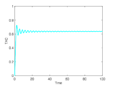
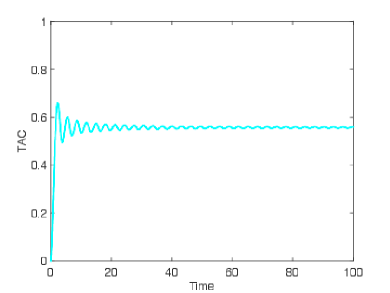
Figure 9: Long time behaviour of time-averaged coherence for a Hamiltonian that optimizes $F(\theta,\tau)$ in a dimer. The left panel shows $\overline{C}_{l_{1}}^{s}(\theta,t)$ and the right panel shows $\overline{C}_{\rm{REOC}}^{s}(\theta,t)$ .

. .

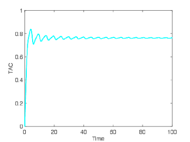
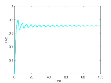
Figure 10: Long time behaviour of time-averaged coherence for a Hamiltonian that optimizes $\overline{C}^{s}(\theta,t)$ in a dimer. The left panel shows $\overline{C}_{l_{1}}^{s}(\theta,t)$ and the right panel shows $\overline{C}_{\rm{REOC}}^{s}(\theta,t)$.

Simulation of the long-term behaviour of $\overline{C}_{l_{1}}^{s}(\theta,t)$ and $\overline{C}_{{\rm{REOC}}}^{s}(\theta,t)$ for the parameter values that optimize $F(\theta,\tau)$ and $\overline{C}^{s}(\theta,t)$ are shown in figures 9 and 10, respectively. The trend towards an asymptotic value is clearly visible in each case.

. .

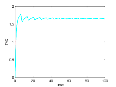
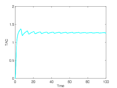
Figure 11: Long time behaviour of time-averaged coherence for a Hamiltonian that optimizes $\overline{C}^{s}(\vec{h},t)$ in a trimer. The left panel shows $\overline{C}_{l_{1}}^{s}(\vec{h},t)$ and the right panel shows $\overline{C}_{\rm{REOC}}^{s}(\vec{h},t)$.

The long-term behaviour of $\overline{C}_{l_{1}}^{s}(\vec{h},t)$ and $\overline{C}_{{\rm{REOC}}}^{s}(\vec{h},t)$ for parameter values optimizing $\overline{C}^{s}(\vec{h},t)$ in the trimer is shown in figure 11. We note a trend towards an asymptotic value also in the trimer case.

7 Conclusions

In this study we have numerically investigated the relation between efficient population transfer and coherence - in different bases and quantified by different coherence measures - in a dimer and trimer system undergoing Schrödinger evolution. Optimization has been performed over a parameter space defined by the site energies and inter-site couplings of a tight-binding Hamiltonian. A possible realization of such a system could be a molecular aggregate of chromophores occupying the sites and being described as two-level systems.

We have found several relations between the efficiency and coherence measures used to study the population transfer process. We summarize these findings as follows:

• The maximum of the time-local coherence and the population transfer in the dimer case occur simultaneously for a maximal transfer efficiency below a certain threshold value. Above this value the coherence maximum precedes the fidelity maximum. For perfect population transfer, the coherence becomes maximal at precisely halfway before and vanishes at the completion of the transfer. Thus, efficient population transfer is characterized by a time-local coherence fully localized before the transfer has been completed.

• It has been shown that in neither the dimer nor the trimer do the parameter values of maximal time-averaged coherence in the site basis coincide with the parameter values corresponding to perfect population transfer between the end-sites. In other words, the efficiency and time-averaged coherence order the Hamiltonians differently with respect to their ability to transfer population.

• In the dimer, the population transfer efficiency is in one-to-one correspondence with coherence in the exciton basis. Thus, perfect population transfer coincides with the upper bounds of the coherence. In this sense, coherence in the exciton basis is directly linked to the efficiency of the population transfer. In the trimer system, the time-averaged coherence in the exciton basis is about $95\%$ of its upper bound at perfect population transfer; thus, the one-to-one correspondence between efficiency and coherence seems to be restricted to the dimer case.

• Optimal efficiency and time-averaged coherence in the site basis do not in general coincide in time. Hence, maximal efficiency and maximal time-averaged coherence are not obtained simultaneously in a system without environmental interactions. This result indicates that coherence in the site basis on its own plays no immediate role for efficient population transfer.

The present analysis can be extended to more sites and environmental effects. This would make it possible to examine the potential impact of quantum coherence on the efficiency of population transport in various systems, such as EET in photosynthetic complexes, under realistic systems. The possibility of a multitude of pathways in such systems would lead to a rich interplay between tunneling and interference effects that can be analyzed and understood by quantifying the coherence during the time evolution.

The related problem of transferring quantum states in spin networks to communicate quantum information between quantum registers has attracted considerable attention in the past [36, 37]. It would be of interest to examine the role of coherence in such processes, in particular to study the optimization of coherence in relation to the state transfer fidelity.

References

References

- [1] Åberg J 2006 Quantifying superposition arXiv:quant-ph/0612146
- [2] Baumgratz T, Cramer M and Plenio M P 2014 Quantifying coherence Phys. Rev. Lett. 113 140401
- [3] Singh U, Bera M N, Misra A, and Pati A K 2015 Erasing quantum coherence: an operational approach arXiv:1506.08186
- [4] Singh U, Bera M N, Dhar H S, and Pati A K 2015 Maximally coherent mixed states: Complementarity between maximal coherence and mixedness Phys. Rev. A 91 052115
- [5] Girolami D 2014 Observable measure of quantum coherence in finite dimensional systems Phys. Rev. Lett. 113 170401
- [6] Winter A and Yang D 2016 Operational resource theory of coherence Phys. Rev. Lett. 116 120404
- [7] Napoli C, Bromley T R, Cianciaruso M, Piani M, Johnston N, and Adesso G 2016 Robustness of coherence: An operational and observable measure of quantum coherence Phys. Rev. Lett. 116 150502
- [8] Rana S, Parashar P, and Lewenstein M 2016 Trace-distance measure of coherence Phys. Rev. A 93 012110
- [9] Streltsov A, Singh U, Dhar H S, Bera M N, and Adesso G 2015 Measuring quantum coherence with entanglement Phys. Rev. Lett. 115 020403
- [10] Chitambar E, Streltsov A, Rana S, Bera M N, Adesso G, and Lewenstein M 2016 Assisted distillation of quantum coherence Phys. Rev. Lett. 116 070402
- [11] Chitambar E and Hsieh M-H 2016 Relating the resource theories of entanglement and quantum coherence Phys. Rev. Lett. 117 020402
- [12] Shao L-H, Xi Z, Fan H, and Li Y 2015 Fidelity and trace-norm distances for quantifying coherence Phys. Rev. A 91 042120
- [13] Streltsov A, Adesso G, and Plenio M B 2016 Quantum coherence as a resource arXiv:1609.02439
- [14] Lostaglio M, Jennings D, and Rudolph T 2015 Description of quantum coherence in thermodynamic processes requires constraints beyond free energy Nat. Commun. 6 6383
- [15] Kim O, Deb P, and Beige A 2015 Cavity-mediated collective laser-cooling of an atomic gas inside an asymmetric trap arxiv:1506.02910
- [16] Korzekwa K, Lostaglio M, Oppenheim J, and Jennings D 2016 The exctraction of work from quantum coherence New. J. Phys. 18 023045
- [17] Misra A, Singh U, Bhattacharya S, and Pati A K 2016 Energy cost of creating quantum coherence Phys. Rev. A 93 052335
- [18] Chen H-B, Chiu P-Y, and Chen Y-N 2016 Vibration-induced coherence enhancement of the performance of a biological quantum heat engine Phys. Rev. A 94 052101
- [19] Creatore C, Parker M A, Emmott S, and Chin A W 2013 Efficient biologically inspired photocell enhanced by delocalized quantum states Phys. Rev. Lett. 111 253601
- [20] Zhang Y, Oh S, Alharbi F H, Engel G, and Kais S 2015 Delocalized quantum states enhance photocell efficiency Phys. Chem. Chem. Phys. 17 5743
- [21] Chain R K and Arnon D I 1977 Quantum efficiency of photosynthetic energy conversion Proc. Natl. Acad. Sci. 74 3377
- [22] Engel G S, Calhoun T R, Read E L, Ahn T-K, Mancal T, Cheng Y-C, Blankenship R E, and Fleming G R 2007 Evidence for wavelike energy transfer through quantum coherence in photosynthetic systems Nature 446 782
- [23] Grover L K 1997 Quantum mechanics helps in searching for a needle in a haystack Phys. Rev. Lett. 79 325
- [24] Plenio M B and Huelga S F 2008 Dephasing-assisted transport: quantum networks and biomolecules New J. Phys. 10 113019
- [25] Mohseni M, Rebentrost P, Lloyd S, and Aspuru-Guzik A 2008 Environment-assisted quantum walks in photosynthetic energy transfer J. Chem. Phys. 129 174106
- [26] Caruso F, Chin A W, Datta A, Huelga S F, and Plenio M B 2009 Highly efficient energy excitation transfer in light-harvesting complexes: The fundamental role of noise-assisted transport J. Chem. Phys. 131 105106
- [27] Chin A W, Datta A, Caruso F, Huelga S F, and Plenio M B 2010 Noise-assisted energy transfer in quantum networks and light-harvesting complexes New J. Phys. 12 065002
- [28] Wu J, Liu F, Shen Y, Cao J, and Silbey R J 2010 Efficient energy transfer in light-harvesting systems I: optimal temperature, reorganization energy and spatial-temporal correlations New. J. Phys. 12 105012
- [29] Irish E K, Gómez-Bombarelli R, and Lovett B W 2014 Vibration-assisted-resonance in photosynthetic exctitation-energy transfer Phys. Rev. A 90 012510
- [30] Rebentrost P, Mohseni M, and Aspuru-Guzik A 2009 Role of quantum coherence and environmental fluctuations in chromophoric energy transport J. Phys. Chem. 113 9942
- [31] Hayes D, Panitchayangkoon G, Fransted K A, Caram J R, Wen J, Freed K F, and Engel G S 2010 Dynamics of electronic dephasing in the Fenna-Matthews-Olson complex New. J. Phys. 12 065042
- [32] Panitchayangkoon G, Hayes D, Fransted K A, Caram J R, Harel E, Wen J, Blankenship R E, and Engel G S 2010 Long-lived quantum coherence in photosynthetic complexes at physiological temperature Proc. Natl. Acad. Sci. 107 12766
- [33] Panitchayangkoon G, Voronine D V, Abramavicius D, Caram J R, Lewis N H, Mukamel S, and Engel G S 2011 Direct evidence of quantum transport in photosynthetic light-harvesting complexes Proc. Natl. Acad. Sci. 108 20908
- [34] Greentree A D, Cole J H, Hamilton A R, and Hollenberg L C L 2004 Coherent electronic transfer in quantum dot systems using adiabatic passage Phys. Rev. B 70 235317
- [35] Schreiber A, Cassemiro K N, Potocek V, Gabris A, Mosley P J, Andersson E, Jex I, and Silberhom C 2010 Photons walking the line: A quantum walk with adjustable coin operations Phys. Rev. Lett. 104 050502
- [36] Bose S 2007 Quantum communication through spin chain dynamics: an introductory overview Contemp. Phys. 48 13
- [37] Kay A 2010 A review of perfect state transfer and its application as a constructive tool Int. J. Quantum Inf. 8 641
- [38] Hemmig E A, Creatore C, Wünsch B, Hecker L, Mair P, Parker M A, Emmott S, Tinnefeld P, Keyser U F, and Chin A W 2016 Programming light-harvesting efficiency using DNA origami Nano Lett. 16 2369
- [39] Woller J G, Hannestad J K, and Albinsson B 2013 Self-assembled nanoscale DNA-porphyrin complex for artificial light harvesting J. Am. Chem. Soc. 135 2759
- [40] Renger T, May V, and Kühn O 2001 Ultrafast excitation energy transfer dynamics in photosynthetic pigment-protein complexes Phys. Rep. 343 137
- [41] Nielsen M A and Chuang I L 2010 Quantum Computation and Quantum Information (Cambridge, UK: Cambridge University Press)
- [42] Lostaglio M, Korzekwa K, Jennings D, and Rudolph T 2015 Quantum Coherence, Time-Translation Symmetry, and Thermodynamics Phys. Rev. X 5 021001
- [43] Horn R A and Johnson C R 1991 Matrix Analysis (Cambridge, UK: Cambridge University Press)
- [44] Cheng S and Hall M J W 2015 Complementarity relations for quantum coherence Phys. Rev. A 92 042101
- [45] Bai Z and Du S 2015 Maximally coherent states Quantum Inf. Comput. 15 1355
- [46] Wootters W K 1998 Entanglement of formation of an arbitrary state of two qubits Phys. Rev. Lett. 80 2245
- [47] Sarovar M, Ishizaki A, Fleming G R, and Whaley K B 2010 Quantum entanglement in photosynthetic light-harvesting complexes Nat. Phys. 6 462
- [48] Hu X-M and Peng J-S 2000 Quantum interference from spontaneous decay in systems: realization in the dressed-state picture J. Phys. B: At. Mol. Phys. 33 921