Clock Monte Carlo methods

Abstract

We propose the clock Monte Carlo technique for sampling each successive chain step in constant time. It is built on a recently proposed factorized transition filter and its core features include its O(1) computational complexity and its generality. We elaborate how it leads to the clock factorized Metropolis (clock FMet) method, and discuss its application in other update schemes. By grouping interaction terms into boxes of tunable sizes, we further formulate a variant of the clock FMet algorithm, with the limiting case of a single box reducing to the standard Metropolis method. A theoretical analysis shows that an overall acceleration of ${\rm O}(N^{\kappa})$ ($0\!\leq\!\kappa\!\leq\!1$) can be achieved compared to the Metropolis method, where $N$ is the system size and the $\kappa$ value depends on the nature of the energy extensivity. As a systematic test, we simulate long-range O$(n)$ spin models in a wide parameter regime: for $n\!=\!1,2,3$, with disordered algebraically decaying or oscillatory Ruderman-Kittel-Kasuya-Yosida-type interactions and with and without external fields, and in spatial dimensions from $d\!=\!1,2,3$ to mean-field. The O(1) computational complexity is demonstrated, and the expected acceleration is confirmed. Its flexibility and its independence from the interaction range guarantee that the clock method would find decisive applications in systems with many interaction terms.

Markov-chain Monte Carlo methods (MCMC) are powerful tools in many branches of science and engineering Ceperley_1995 ; Frenkel_1996 ; Landau_2000 ; Opplestrup_2006 ; Rogers_2006 ; Robert_2001 ; Liu_2001 ; Glasserman_2004 . For instance, MCMC plays a crucial role in the recent success of AlphaGo AlphaGo , and appears as a keystone of the potential next deep learning revolution Neal_1996 ; Ghahramani_2015 . To estimate high-dimensional integrals, MCMC generates a chain of random configurations, called samples. The stationary distribution is typically a Boltzmann distribution and the successive moves depend on the induced energy changes. Despite a now long history, the most successful and influential MCMC algorithm remains the founding Metropolis algorithm Metropolis_1953 for its generality and ease of use, ranked as one of the top 10 algorithms in the 20th century Dongarra_2000 .

The Metropolis algorithm has, however, two major limitations. First, nearby samples can be highly correlated and, around the phase transition, the simulation efficiency drops quickly as the system size $N$ increases. Second, an attempted move requires calculating the induced total energy change, leading to expensive computational complexities of up to O$(N)$ for systems with long-range interactions. This issue is also very acute in machine learning, where likelihood evaluations Bardenet_2015 scale with the number of data points.

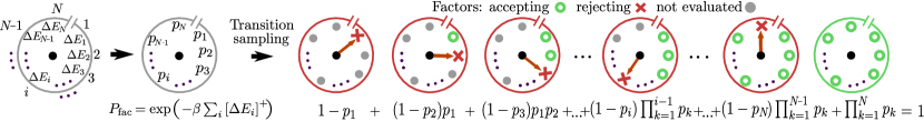
Figure 1: Sketch of the clock sampling technique. The inhomogeneous Bernoulli process described by Eq. (2) can be decomposed into $N\!+\!1$ clocks, where the $i$th clock ($i\!\leq\!N$) alarms of the first occurrence of a rejection event at time $i$ and the $(N\!+\!1)$th clock, with no alarm, represents an acceptance event. Such a process can be sampled within O(1) computational complexity.

Enormous efforts have been devoted to circumventing the two limitations. Various efficient update schemes have been designed, including the celebrated cluster and worm algorithms Swendsen_1987 ; Wolff_1989 ; Prokofev_2001 , and the event-chain (EC) irreversible method Bernard_2009 ; Michel_2014 . Several techniques are also available in reducing the computational complexity for specific algorithms and systems. An “early-rejection” scheme was mentioned in the textbook Frenkel_1996 , which is nevertheless of O$(N)$ complexity. Making use of the particular feature that each bond is treated independently in the cluster-update scheme Edwards_1988 , Luijten and Blöte Luijten_1995 applied an efficient sampling procedure to place occupied bonds, instead of visiting each bond sequentially and throwing a random number to decide its status. The Luijten-Blöte cluster algorithm has O(1) complexity Luijten_1995 ; Fukui_2008 ; Flores_2017 , and has been generalized to quantum systems Deng_2002 . Recently, an EC algorithm was proposed for long-range soft-sphere systems Kapfer_2016 .

In this Rapid Communication, we propose a general “clock” MC method, which has a constant-time sampling and can be applied to various update schemes. The core ingredient is the factorized Metropolis filter proposed in Ref. Michel_2014 . In particular, an algorithm of O(1) computational complexity is formulated in the framework of the local and most general update scheme, which we call the clock factorized Metropolis (FMet) algorithm. By grouping the interaction terms into boxes of tunable sizes, we further obtain a variant of the clock FMet algorithm for efficiency optimization. The limiting case of a single box recovers the Metropolis method, directly illustrating the generality of the clock FMet algorithm. We also discuss how the clock technique acts as a common ground for existing exact complexity reduction methods and present in particular its implementation in the EC update scheme.

While gaining an O$(N)$ speeding-up in computational effort, the clock FMet algorithm can suffer from a lower acceptance probability than the Metropolis method. The overall acceleration comes from the compromise of these two effects. We provide a systematic performance analysis by classifying the system into three types of strict, marginal and sub-extensivities, and show that an overall acceleration can be achieved up to O($N$) for the strict extensivity and O($N^{\kappa}$) (1$>\!\kappa\!\geq$0) for the other two. As other exact complexity reduction methods belong to the algorithmic clock class, this analysis also applies to these techniques. Finally, we extensively simulate long-range O$(n)$-spin models in a wide parameter regime: for $n\!=\!1,2,3$, with disordered algebraically decaying or oscillatory Ruderman-Kittel-Kasuya-Yosida (RKKY)-type interactions, with and without external fields and in spatial dimensions from $d\!=\!1,2,3$ to mean-field. The O(1) computational complexity is demonstrated, and the expected acceleration is confirmed. These achievements are based on the complementary combination of the factorized Metropolis filter, O(1) sampling procedures and the grouping trick.

Clock FMet algorithm. Consider a system described by a collection of states $\mathcal{S}$ with Boltzmann weights $\pi(\mathcal{S})\propto\exp(-\beta E(\mathcal{S}))$, with $\beta=1/k_{\rm b}T$ the inverse temperature. The energy $E(\mathcal{S})=\sum_{i}E_{i}(\mathcal{S})$ is the sum of all interaction terms that are pairwise or more generally in many-body groups. At each step, the Metropolis algorithm attempts to update a state $\mathcal{S}$ into another $\mathcal{S}^{\prime}$ with acceptance probability

$$P_{\rm Met}=\min\left(1,\frac{\pi(\mathcal{S}^{\prime})}{\pi(\mathcal{S})}\right)=\exp(-\beta\left[\Delta E_{\rm tot}\right]^{+})$$ (1)

with $[x]^{+}=\max(0,x)$. Evaluating the induced energy change $\Delta E_{\rm tot}\!\equiv\!\sum_{i}\Delta E_{i}$ requires a costly computation of all the involved interactions. Therefore, we focus now on the factorized Metropolis filter Michel_2014

$$P_{\rm fac}=\prod_{i}p_{i}(\mathcal{S}\to\mathcal{S}^{\prime})=\prod_{i}\exp(-\beta\left[\Delta E_{i}\right]^{+})\;,$$ (2)

which also satisfies the detailed-balance condition $\pi(\mathcal{S})p(\mathcal{S}\!\!\to\!\mathcal{S}^{\prime})=\pi(\mathcal{S}^{\prime})p(\mathcal{S}^{\prime}\!\!\to\!\mathcal{S})$. Hereinafter we omit the dependence on $\mathcal{S}\!\!\to\!\mathcal{S}^{\prime}$ except in case it hinders the clarity. The factorized filter is a key component of the recent EC methods, as it allows one to extract interesting system symmetries. On a more general level, the factorization of transition rates can also play an important physical role in dynamical studies Hucht_2009 . A crucial feature of Eq. (2) is the consensus rule: As the transition probability $P_{\rm fac}$ is a product of independent factors $p_{i}$, an attempted move is accepted only if all the factors give permission (Fig. 1). This leads to a lower acceptance probability in Eq. (2) than in Eq. (1). However, we show here how it plays a key role in designing the clock technique that dramatically reduces the computational complexity from O$(N)$ to O(1), greatly improving the overall performance.

Without loss of generality, we illustrate the clock FMet method in the example of a long-range O$(n)$ model of $N\!+\!1$ spins, with the Hamiltonian

$$\mathcal{H}=-c(N)\sum_{i<j}J_{ij}\boldsymbol{S}_{i}\cdot\boldsymbol{S}_{j}\;,\hskip 14.22636pt(|\boldsymbol{S}|=1)$$ (3)

with $\boldsymbol{S}$ unit vectors in $\mathbb{R}^{n}$. For $n\!=\!1,2,3$, one has the Ising, XY and Heisenberg models, respectively. The coupling strength $J_{ij}$ depends on distance $r_{ij}$, and can be ferromagnetic ($J_{ij}\!>\!0$), anti-ferromagnetic ($J_{ij}\!<\!0$), or disordered. There are in total $N(N\!+\!1)/2$ interaction terms. The normalization constant $c(N)$, scaling typically in $1/N^{\alpha}$ ($1\!\geq\!\alpha\!\geq\!0$), is to ensure the energy extensivity, which, e.g., is $1/N$ for a mean-field ferromagnet but $1/\sqrt{N}$ for the Sherrington-Kirkpatrick model Sherrington_1975 ; Kirkpatrick_1978 . An attempted move is to flip or rotate a randomly-chosen spin $\boldsymbol{S}_{j}$. This leads to an energy change $-c(N)\sum_{i\neq j}J_{ij}(\boldsymbol{S}^{\prime}_{j}-\boldsymbol{S}_{j})\cdot\boldsymbol{S}_{i}$, which requests an O$(N)$ computation in the Metropolis algorithm.

A straightforward implementation of Eq. (2) is as follows. One orders the factor terms from $i\!=\!1$, sequentially samples the rejection of each factor $i$ with probability $1-p_{i}$, and stops at the first-rejecting factor $i_{\rm rej}$; if no rejection is sampled until factor $N$, the move is accepted. This is analogous to an inhomogeneous Bernoulli process of rate $p_{i}$, as illustrated in Fig. 1, where the $i$th clock, with probability $P_{\text{rej}}(i)\!=\!(1-p_{i})\prod_{k=1}^{i-1}p_{k}$, represents the event for the $i$th factor to be first-rejecting. Instead of sequentially sampling each factor, one can also evaluate cumulative probability $F_{k}\!=\!\sum_{k^{\prime}=1}^{k}P_{\text{rej}}(k^{\prime})$ and directly obtain the $i_{\rm rej}\!=\!i$ value by solving $F_{i-1}\!<\!\nu\!\leq\!F_{i}$ with a single random number $\nu\!\in\!(0,1]$. Nevertheless, the individual probabilities $p_{k}$ depend a priori on a local configuration $(\boldsymbol{S}_{i},\boldsymbol{S}_{j})$, and each move still requires an average number $\mathcal{C}\!\sim\!{\rm O}(N)$ of $p_{k}$-evaluations.

To avoid these costly evaluations, we introduce a bound Bernoulli process with a configuration-independent probability $\widehat{p_{i}}$, so that $1-\widehat{p_{i}}\geq 1-p_{i}(\mathcal{S}\!\!\!\to\!\!\mathcal{S}^{\prime})$, as done in Ref. Luijten_1995 . An actual rejection at a factor $i$ corresponds to a bound rejection once resampled with relative probability

$$p_{i,{\rm rel}}=(1-p_{i})/(1-\widehat{p_{i}})\;.$$ (4)

At each factor $i$, three events are possible: (${\rm A}_{1}$) bound acceptance with $p_{i}^{{\rm A}_{1}}\!=\!\hat{p}_{i}$, ($\rm A_{2}$) bound rejection and resampling rejection with $p_{i}^{{\rm A}_{2}}\!=\!(1-\hat{p}_{i})(1-p_{i,{\rm rel}})$, and (R) bound rejection and resampling acceptance with $p_{i}^{{\rm R}}\!=\!(1-\hat{p}_{i})p_{i,{\rm rel}}$. Sampling the $i$th clock, i.e. the first-rejection at factor $i$, is then replaced by sampling a random path of events (${\rm A}_{1}$) or (${\rm A}_{2}$) for $k\!\leq\!i\!-\!1$ and a first event (R) at $i$, as described by

$$P_{\text{rej}}(i)=p_{i}^{{\rm R}}\prod_{k=1}^{i-1}(p_{k}^{{\rm A}_{1}}+p_{k}^{{\rm A}_{2}})\;.$$ (5)

As the bound $\hat{p}_{i}$’s are configuration-independent, the bound cumulative probabilities $\widehat{F}_{i}$ can be analytically calculated or tabulated. Initializing $i_{\widehat{\rm rej}}\!=\!0$, the next bound rejection $i_{\widehat{\rm rej}}$ is updated to $i$ by solving,

$$\widehat{F}_{i-1}<\nu(1-\widehat{F}_{i_{\widehat{\rm rej}}})\!+\!\widehat{F}_{i_{\widehat{\rm rej}}}\leq\widehat{F}_{i}\;,$$ (6)

and the resampling is then applied. This is done within an O$(1)$ complexity. If no actual rejection occurs, i.e. event (${\rm A}_{2}$), the procedure is repeated until an event (R) (actual rejection) is sampled or until $\nu(1-\widehat{F}_{i_{\widehat{\rm rej}}})\!+\!\widehat{F}_{i_{\widehat{\rm rej}}}>\widehat{F}_{N}$ (actual acceptance). The overall complexity $\mathcal{C}$ identifies now with the average number of attempted bound rejections $\!\sim\!{\rm O}(\ln P_{B}/\ln P_{\rm Fac})\!\sim\!{\rm O}(1)$ if the bound consensus probability $P_{B}\!=\!\prod\widehat{p}_{i}$ scales with $N$ as $P_{\rm Fac}$. For a homogeneous case $\widehat{p}_{i}\!\equiv\!\widehat{p}$, Eq. (6) reduces to $i=i_{\widehat{\rm rej}}\!+\!\left\lfloor 1\!+\!\ln(\nu)/\ln(\widehat{p})\right\rfloor$, which can be easily adapted to inhomogeneous bound probabilities by ordering the factors increasingly with $\widehat{p}_{i}$ and by replacing $\widehat{p}$ by $\widehat{p}_{i_{\widehat{\rm rej}}+1}$ Shanthikumar_1985 . Alternatively, one can directly generate the whole list of bound rejection events by the Walker method Walker_1977 ; Marsaglia_2004 or its Fukui-Todo extension Fukui_2008 , and then sequentially apply the resampling.

Algorithm 1 summarizes a clock FMet method for a long-range spin system. For Hamiltonian (3), $\widehat{p}_{k}$ can be taken as a function of distance $r_{ij}$ as $\widehat{p}(r_{ij})\!=\!\exp(-2\beta c(N)|J_{ij}|)$.

Draw a random spin $j$ and a random move $\boldsymbol{S}_{j}\!\!\to\!\boldsymbol{S}_{j}^{\prime}$

$i_{\widehat{\rm rej}}\leftarrow 0$ $\triangleright$ Sample bound rejections starting from $i_{\widehat{\rm rej}}$

while True do

     $i_{\widehat{\rm rej}}\leftarrow i$ $\triangleright$ Next bound rejection $i$ given by Eq. (6)

     if $i_{\widehat{\rm rej}}\!>\!N$ then

         $\boldsymbol{S}_{j}\leftarrow\boldsymbol{S}^{\prime}_{j}$ $\triangleright$ Move accepted

         Break

     else$\triangleright$ Decide whether it is an actual rejection

         $p_{i_{\widehat{\rm rej}},{\rm rel}}\leftarrow$ Eq.(4)

         if $\text{ran}(0,1)\leq p_{i_{\widehat{\rm rej}},{\rm rel}}$ then

              Break$\triangleright$ Move rejected               

Algorithm 1 Clock factorized Metropolis (Clock FMet)

The clock method can be applied to any transition probability expressed as a product of independent factors, as the one proposed in Hucht_2009 for instance. However, the factorized Metropolis filter, in addition to a maximal acceptance rate factorwise, presents the following advantage. As each factor in Eq. (2) can contain an arbitrary number of interactions, we introduce a variant of clock FMet algorithm in which the interactions are grouped into “boxes” b of tunable sizes $B_{b}$, as

$$P^{\text{Box}}_{\rm fac}\!=\!\prod_{b}\exp\left(-\beta\left[\sum_{i=1}^{B_{b}}\Delta E_{b_{i}}\right]^{+}\right).$$ (7)

It leads to new optimization possibilities (e.g. how to group the interaction terms). If all the interactions are in a single box, one recovers the standard Metropolis method.

The clock technique has two important ingredients: the consensus rule and the resampling. Both the ingredients are general: They do not depend either on any specific configurations, or on factor ordering, or on energy functions, or on update schemes. For systems in a continuous volume, as soft spheres, one can introduce a grid Kapfer_2016 to which the clock technique is applied.

Generalization to other update schemes. We illustrate the generality of the clock method by discussing its application in the EC method for the O($n$) spin model with $n\!\geq\!2$. Michel_2015 ; Nishikawa_2015 . With an auxiliary lifting variable $j$ that specifies the moving spin, the EC method proposes to rotate infinitesimally its angle as $\phi_{j}\!\!\to\!\phi_{j}\!+\!{\rm d}\phi$. Such a move is rejected by at most one spin $i$, owing to a continuous derivation of Eq. (2). This yields $p_{i}\to 1-\lambda_{i}{\rm d}\phi$ and $P_{\text{rej}}(i)\to\lambda_{i}{\rm d}\phi$. For each factor $i$, the rejection event, with distance $\delta_{i}\phi$, is thus ruled by a Poisson process (PP) of rate $\lambda_{i}$, continuous derivation of the standard Bernoulli process. The spin $j$ is then rotated by the minimum distance $\delta\phi=\min(\delta_{i}\phi)$, and the associated factor becomes the moving spin, i.e. $j\!\!\to\!i_{\rm min}$. For long-range interactions, evaluating $\delta_{i}\phi$ for all the factors becomes costly.

To derive the clock method, we introduce a bound Poisson process of total rate $\bar{\lambda}=\sum\bar{\lambda}_{i}\;(\bar{\lambda}_{i}\geq\lambda_{i})$, evaluate a random bound rotation $\delta\widehat{\phi}\!=\!-\ln\nu/\bar{\lambda}$, sample the rejecting bound factor $i_{\widehat{\rm min}}=i$ with probability $\bar{\lambda}_{i}/\bar{\lambda}$, and resample it as an actual lift $j$ to $i$ according to $\lambda_{i}/\bar{\lambda}_{i}$ (Eq. (4)). This comes down to the thinning method Lewis_1979 , already applied for soft-sphere systems Kapfer_2016 and for logistic regression in machine learning Bouchard_2016 .

We also note that the cluster methods Swendsen_1987 ; Wolff_1989 factorize each interaction term independently as in Eq. (2). The resampling procedures in the extended cluster algorithms for long-range interactions and for quantum spin systems Luijten_1995 ; Fukui_2008 ; Flores_2017 ; Deng_2002 can be understood as specific cases of the clock method.

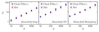
Figure 2: Integrated autocorrelation time $\tau_{E}$ of the energy for the ferromagnetic mean-field $O(n)$ model expressed in units of system sweeps. The values for the clock FMet algorithm are normalized by $\gamma$ (Eq. (8)).

Performance analysis. We expect and numerically confirm in Fig. 2 that the standard Metropolis and the clock FMet algorithms have the same physical dynamics. The overall acceleration $\mathcal{A}$ in the latter comes then from the speeding-up in the complexity $\mathcal{C}$, corrected by the slowing-down $\gamma$ due to a lower acceptance in the factorized filter (2), leading to $\mathcal{A}\!\sim\!$ O$(N/\mathcal{C}\gamma)$. Both effects can be characterized by the scaling of $\sum_{i}\max|\Delta E_{i}|$ and $\sum_{i}|\Delta E_{i}|$, as $\gamma=P_{\rm Met}/P_{\rm Fac}$ can be written as

$$\ln\gamma\!=\!\frac{\beta}{2}\left(\sum_{i}|\Delta E_{i}|-|\sum_{i}\Delta E_{i}|\right)\;,$$ (8)

and as $\mathcal{C}\!\sim\!\ln P_{B}/\ln P_{\rm Fac}\!\sim\!\sum_{i}\max|\Delta E_{i}|/\sum_{i}|\Delta E_{i}|$. Depending on the nature of the energy extensivity and phase of the system, the sum $\sum_{i}|\Delta E_{i}|$ may diverge as size $N\!\!\to\!\infty$, while the sum $|\sum_{i}\Delta E_{i}|$ converges to a constant. This normally occurs in disordered systems with slowly decaying interactions, in which the “satisfied” and “unsatisfied” interaction terms compensate each other. The divergence of $\gamma$ can be controlled by introducing enough compensation through boxes. For a constant size $B$, it increases the complexity to O($B|\ln P_{B}|$), but leads to an acceleration $\sim\!{\rm O}(N/(B|\ln P_{B}|)$). By definition, $B\!\propto\!N$ would ensure a maximal energy compensation but an O(1) acceleration.

We classify the system into the three types of strict, marginal and sub- extensivities, for which $\sum_{i}\max|\Delta E_{i}|$ respectively scales as O(1), O($\ln N$) and O($N^{\alpha}$) ($1\!\geq\!\alpha\!>\!0$). We demonstrate that the clock FMet method of tunable constant box sizes $B$ might achieve an overall acceleration

• $\mathcal{A}\!\sim\!$ O$(N)$ for strict extensivity, directly from $\gamma\!\sim\!$ O(1) and $\mathcal{C}\!\sim\!{\rm O}(1)$.

• $\mathcal{A}\!\sim$O$(N^{\kappa})$ (0$\leq\!\kappa\!<$1) for sub-extensivity. Depending on the phase, $\ln\gamma$ may diverge, up to $N^{\alpha}$. For the spin glass of algebraically decaying interaction as $1/r^{\sigma}$ ($\sigma\!<\!1$), we find that a box size $B\propto N/N^{\omega}$, with a fine-tuning exponent $0\!\leq\!\omega\!<\!1$, gives a sufficient compensation and an O$(N^{\kappa}$) ($\kappa\!\sim\![\omega-\alpha]^{+}$) acceleration.

• ${\rm O}(N/(\ln N)^{2})\!\leq\!\mathcal{A}_{\rm margin}\!\leq\!{\rm O}(N/\ln N)$ for marginal extensivity. We observe that setting $B$ up to $\ln N$ can be necessary to control $\gamma$.

For frustrated systems, irrespective of which class they belong to, efficient cluster algorithms are normally unavailable due to the huge cluster sizes. Given the substantial acceleration for all the three classes of strict, marginal, and sub-extensivities, the application of the clock FMet method is very promising.

Simulations. We simulate three typical systems in statistical physics, including long-range Ising spin glass, the disordered O$(n)$ model with random external fields, and the O$(n)$ model with RKKY-type interactions. We record the number of energy evaluations $\mathcal{C}$ for each MC step, which for the Metropolis method is simply $\mathcal{C}\!=\!N$. We measure the integrated correlation times $\tau$ for magnetic susceptibility $\chi$ in the units of energy evaluations, and compute the overall acceleration $\mathcal{A}$ as the inverse ratio $\mathcal{A}\!=\!\tau_{\rm other}/\tau_{\rm FMet}$, where $\tau_{\rm other}$ is for the Metropolis or the Luijten-Blöte (LB) cluster method. For the Metropolis method, it comes down to $\mathcal{A}\!=\!N/(\gamma\mathcal{C})$.

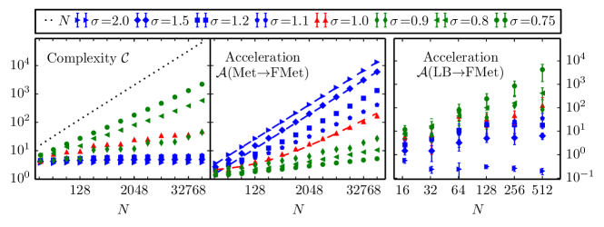
Figure 3: Complexity $\mathcal{C}$ (left) and acceleration $\mathcal{A}$ for the clock FMet algorithm for the 1D ($\beta\!=\!1$) long-range Ising spin glass, compared to the Metropolis algorithm (middle) and the LB algorithm (right). The dashed blue and red lines respectively represent fits to $aN$ and $aN/(\log N)^{2}+b$.

Long-range Ising spin glass. We consider a periodic one-dimensional (1D) spin glass defined by Eq. (3). The interactions decay algebraically as $J_{ij}=s_{ij}/r_{ij}^{\sigma}$ ($\sigma\!>\!0$), with $s_{ij}=\pm 1$ from a bimodal distribution. The normalization $c(N)$ is given by $c(N)^{-2}\!=\!\sum_{j>1}\left\langle J_{1j}^{2}\right\rangle$. This system, with a tunable exponent $\sigma$, is particularly useful in revealing the crossover behavior from the low-dimensional to the mean-field spin glass Kotliar_1983 ; Bray_1986 ; Beyer_2012 . For simplicity, the simulation is made at the mean-field critical temperature $\beta=1$ Sherrington_1975 . Depending on the value of $\sigma$, we recover the three extensivity regimes, i.e. strict ($\sigma\!>\!1$), marginal ($\sigma\!=1$) and sub-extensivities ($\sigma\!<\!1$). We group the interaction terms following respective $r_{ij}$ values and set the box size as $B=2\;(\sigma\!>\!1)$, $\ln N\;(\sigma\!=\!1)$, and $N^{2(1-\sigma)}\;(\sigma\!<\!1)$. The results are shown in Fig. 3. For $\sigma\!>\!1$, the computational complexity $\mathcal{C}$ converges to a constant, and a dramatic overall acceleration $\mathcal{A}\!\sim\!{\rm O}(N)$ is achieved. For $\sigma\!=\!1$, we have $\mathcal{C}\!\sim\!\ln N^{2}$ and a significant acceleration $\mathcal{A}$ converging to $N/(\ln N)^{2}$. For $\sigma\!<\!1$, both $\mathcal{C}$ and $\mathcal{A}$ increase sub-linearly as $N$. The acceleration $\mathcal{A}$ drops as $\sigma$ becomes smaller. Nevertheless, given the simplicity of the clock FMet method, the gained improvement is still significant. We also compare its performances with the LB algorithm, which confirm the superiority of the local Clock FMet for disordered systems. These results are fully consistent with the performance analysis.

RKKY-type interactions. We then consider the 2D and 3D Heisenberg models with oscillatory Ruderman-Kittel-Kasuya-Yosida (RKKY) interactions $J_{ij}\!=\!J_{0}(\cos(2k_{\rm F}r_{ij})/r_{ij}^{d})\exp(-r_{ij}/\lambda)$, where $d$ is the spatial dimension, $k_{\rm F}$ is the Fermi vector ($k_{\rm F}\!\approx\!4.91$ for the spin-glass system $Cu$Mn), and $\lambda$ is the characteristic length in the damping term Bray_1986 ; Matasubara_1992 ; Priour_2005 ; Priour_2006 ; Szalowski_2008 ; Kirkpatrick_2016 . Due to their approximate description of real materials, rich behaviors, and important roles in bridging the experimental study of glassy materials and the spin-glass theory of short-range interactions Bray_1986 ; Matasubara_1992 , these systems are under extensive studies. For simplicity, we set $J_{0}\!=\!1$ and $k_{\rm F}\!=\!\pi$, and take $\lambda\!=\!3$ for 3D and $\lambda\!=\!\infty$ for 2D, so that the system is in the class of strict (3D) and marginal (2D) extensivities. The simulations are at $\beta(2D)\!=\!1$ and $\beta(3D)\!=\!0.693$, close to the critical temperature $\beta_{c}\!=\!0.693\,003(2)$ for the 3D pure Heisenberg model Deng_2005 . Box sizes are set to 1 and the achieved acceleration is again $\mathcal{A}\!\sim$ O$(N)$ for the strict extensivity, and $\mathcal{A}\!\sim$ O$(N/\ln N)$ for the marginal extensivity, as illustrated in Fig. 4.

Disordered random-field model. Finally, we study a disordered mean-field O$(n)$ model in a random external field. The interactions are partly disordered, i.e. $J_{ij}\!=\!1$ for 90% of interactions while the remaining $J_{ij}$ are drawn from a normal distribution with $\langle J_{ij}\rangle\!=\!0$ and $\langle J_{ij}^{2}\rangle\!=\!1$. A quenched random field is applied to each lattice site as $-\boldsymbol{h_{i}}\!\cdot\!\boldsymbol{S_{i}}$, where $\boldsymbol{h_{i}}$ is drawn from an $n-$dimensional normal distribution. The normalization is $c(N)\!=\!1/N$, and the system belongs to the class of strict extensivity. Random-field models have applications in a wide range of physics Larkin_1970 ; Efros_1975 ; Kirkpatrick_1994 ; Sethna_1993 ; Rosinberg_2008 , including the pinning of vortices in superconductors, Coulomb glass, the metal-insulator transition, and hysteresis and avalanche physics. In general spatial dimensions, the thermodynamic properties and phase transitions are still debated Krzakala_2010 ; Leuzzi_2013 . We perform simulations at the mean-field critical temperature $\beta=n$, with box sizes set to 1. The results are shown in Fig. 5. The clock FMet method clearly displays an O$(N)$ acceleration over the Metropolis algorithm for all the Ising, XY and Heisenberg models. It also exhibits some superiority ($\mathcal{A}\sim 50$ for large system sizes) compared to the LB cluster algorithm that already implements the clock technique and has an O(1) computational complexity. The central-limit theorem tells that, as temperature is lowered and/or the strength of the external fields is increased, the acceptance rate exponentially drops for clusters of large sizes in the LB algorithm, and thus this superiority would become more pronounced.

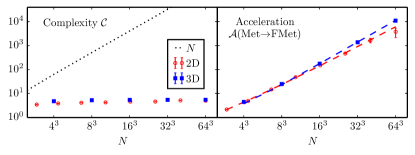
Figure 4: Complexity $\mathcal{C}$ (left) and acceleration $\mathcal{A}$ (right) for the 2D ($\beta\!=\!1$, red circle) and 3D ($\beta\!=\!0.693$, blue square) RKKY Heisenberg spin systems, comparing the clock FMet method to the Metropolis algorithm. The dashed red and blue lines respectively represent fits to $aN$ and $aN/\log N+b$.

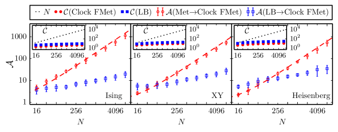
Figure 5: Acceleration $\mathcal{A}$ for the disordered mean-field O$(n)$ model in random fields at $\beta\!=\!n$ (complexity $\mathcal{C}$ in insets). The clock FMet method exhibits important acceleration $\mathcal{A}$, compared to both the Metropolis (red circles) and the LB cluster algorithm (blue squares). The dashed red line represents a fit to $aN+b$.

Conclusion. We introduce a general clock technique with O(1) computational complexity for each Monte Carlo step, and discuss its implementations in various update schemes, regrouping most existing complexity reduction techniques into a single algorithmic class. An important application is the clock FMet algorithm. This is made possible owing to the following three flexible features of the factorized filter (2). First, the consensus rule in Eq. (2) allows for the decision of the fate of a proposed move by an O(1) sampling procedure. Second, the equal generality of Eqs. (1) and (2) allows for a similar application range. Third, the factorization range flexibility given by the grouping trick in Eq. (7) allows for a semi-continuation from the Metropolis Eq. (1) to the factorized filter Eq. (2) and a control over the frustration present in the considered system.

The clock FMet algorithm and its variant with tunable box sizes can lead to significant or even dramatic acceleration $\mathcal{A}$. Depending on the system, theoretical analysis gives $\mathcal{A}$ up to O($N$), O($N/\ln N$) and O($N^{\kappa}$) ($1\!>\!\kappa\!\geq\!0$) for respectively strict, marginal and sub-extensivities. Moreover, as the Metropolis method can be understood as a limiting case of the clock FMet, the latter cannot be worse. This is confirmed by simulations of long-range O$(n)$ models in a wide parameter range. Since these systems are under active studies and the simulations rely heavily on the Metropolis method, the clock FMet algorithm is readily available to explore their rich physics. From its simplicity and ease of use, we conclude that the clock technique is a serious candidate for tackling Monte Carlo scaling in all scientific fields.

References

- (1) D. M. Ceperley, Reviews of Modern Physics 67, 2:279-355 (1995).
- (2) D. Frenkel and B. Smit, Understanding Molecular Simulation - From Algorithms to Applications., Academic Press, San Diego (1996).
- (3) D. P. Landau and K. Binder, A Guide to Monte Carlo Simulations in Statistical Physics, Cambridge University Press, Cambridge (2000).
- (4) T. Opplestrup, V. V. Bulatov, G. H. Gilmer, M. H. Kalos, and B. Sadigh, Phy. Rev. Lett. 97, 230602 (2006).
- (5) D. W. O. Rogers, Phys. Med. Biol 51, R287 (2006).
- (6) C. P. Robert and G. Casella, Monte Carlo Statistical Methods, Springer Texts in Statistics, Springer (1999).
- (7) J. S. Liu, Monte Carlo Strategies in Scientific Computing, Springer Series in Statistics, Springer (2001).
- (8) P. Glasserman, Monte Carlo Methods in Financial Engineering, Springer-Verlag, New York (2004).
- (9) D. Silver, A. Huang, C. J. Maddison, A. Guez, L. Sifre, G. Van Den Driessche, J. Schrittwieser, I. Antonoglou, V. Panneershelvam, M. Lanctot and others, Nature 529, 7587, 484-489 (2016).
- (10) R. M. Neal, Bayesian Learning for Neural Networks, Springer (1996).
- (11) Z. Ghahramani, Nature 521, 7553, 452-459 (2015).
- (12) N. Metropolis, A. W. Rosenbluth, M. N. Rosenbluth, A. H. Teller and E. Teller, J. Chem. Phys. 21, 1087 (1953).
- (13) J. Dongarra and S. Sullivan, Comput. Sci. Eng. 2, 1, 22-23 (2000).
- (14) R. Bardenet, A. Doucet and C. Holmes, JMLR, 18, 1 (2017).
- (15) R. H. Swendsen and J. S. Wang, Phys. Rev. Lett. 58, 86 (1987).
- (16) U. Wolff, Phys. Rev. Lett. 62, 361 (1989).
- (17) N. Prokof’ev and B. Svistunov, Phys. Rev. Lett. 87, 160601 (2001).
- (18) E. P. Bernard, W. Krauth and D. B. Wilson, Phys. Rev. E 80, 056704 (2009).
- (19) M. Michel, S. C. Kapfer and W. Krauth, J. Chem. Phys. 140, 054116 (2014).
- (20) R.G. Edwards and A.D. Sokal, Phys. Rev. D 38, 2009 (1988).
- (21) E. Luijten and H. W. J. Blöte, Int. J. Mod. Phys. C 06, 359 (1995).
- (22) K. Fukui and S. Todo, Journal of Computational Physics 228, 7:2629 - 2642 (2008).
- (23) E. Flores-Sola, M. Weigel, R. Kenna and B. Berche, Eur. Phys. J. Special Topics 226, 581-594 (2017).
- (24) Y. Deng and H. W. J. Blöte, Phys. Rev. Lett. 88, 190602 (2002).
- (25) S. C. Kapfer and W. Krauth, Physical Review E 94, 031302(R) (2016).
- (26) A. Hucht, Phys. Rev. E 80, 061138 (2009).
- (27) D. Sherrington and S. Kirkpatick, Phys. Rev. Lett. 35, 26:1792-1796 (1975).
- (28) S. Kirkpatrick and D. Sherrington, Phys. Rev. B 17, 4384 (1978).
- (29) J.G. Shanthikumar, European Journal of Operational Research 21, 387 (1985).
- (30) A. J. Walker, ACM Trans. Math. Softw. 3, 253 (1977).
- (31) G. Marsaglia, W. W. Tsang and J. Wang, Journal of Statistical Software 11, 1 (2004).
- (32) M. Michel, J. Mayer and W. Krauth, EPL 112, 20003 (2015).
- (33) Y. Nishikawa, M. Michel, W. Krauth and K. Hukushima, Phys. Rev. E 92, 063306 (2015).
- (34) P. A. W. Lewis and G. S. Shedler, Naval Research Logistics 26, 403-413 (1979).
- (35) A. Bouchard-Côté, S. J. Vollmer and A. Doucet, J. Am. Stat. Assoc. 113, 855 (2018).
- (36) G. Kotliar, P. W. Anderson and D. L. Stein, Phys. Rev. B 27, 602(R) (1983).
- (37) A. J. Bray, M. A. Moore and A. P. Young, Phys. Rev. Lett 56, 2641 (1986).
- (38) F. Beyer, M. Weigel and M. A. Moore, Phys. Rev. B 86, 014431 (2012).
- (39) F. Matsubara and M. Iguchi, Phys. Rev. Lett. 68, 3781 (1992).
- (40) D. J. Priour, Jr., E.H. Hwang, and S. Das Sarma, Phys. Rev. Lett. 95, 037201 (2005).
- (41) D. J. Priour, Jr. and S. Das Sarma, Phys. Rev. Lett. 97, 127201 (2006).
- (42) K. Szalowski and T. Balcerzak, Phys. Rev. B 77, 115204 (2008).
- (43) K. Kirkpatrick and T. Nawaz, J. Stat. Phys. 165, 1114 (2016).
- (44) Y. Deng, H. W. J. Blöte and M. P. Nightingale, Phys. Rev. E 72, 016128 (2005).
- (45) A. I. Larkin, Zh. Eksp. Teor. Fiz. 58, 1466 (1970) [Sov. Phys. JETP 31, 784 (1970)].
- (46) A.L. Efros and B.I Shklovskii, J. Phys. C 8, L49 (1975).
- (47) T. R. Kirkpatrick and D. Belitz, Phys. Rev. Lett. 73, 862 (1994).
- (48) J. P. Sethna, K. Dahmen, S. Kartha, J. A. Krumhansl, B. W. Roberts and J. D. Shore ,Phys. Rev. Lett 70, 3347 (1993).
- (49) M. L. Rosinberg, G. Tarjus and F. J. Perez-Reche, J. Stat. Mech., P03003 (2009).
- (50) F. Krzakala, F. Ricci-Tersenghi and L. Zdeborova, Phys. Rev. Lett 104, 207208 (2010).
- (51) L. Leuzzi and G. Parisi, Phys. Rev. B 88, 224204 (2013).