Arrival times of Cox process with independent increments
with application to prediction problems

Abstract.

Properties of arrival times are studied for a Cox process with independent (and stationary) increments. Under a reasonable setting the directing random measure is shown to take over independent (and stationary) increments of the process, from which the sets of arrival times and their numbers in disjoint intervals are proved to be independent (and stationary). Moreover, we derive the exact joint distribution of these quantities with Gamma random measure, whereas for a general random measure the method of calculation is presented. Based on the derived properties we consider prediction problems for the shot noise process with Cox process arrival times which trigger additive processes off. We obtain a numerically tractable expression for the predictor which works reasonably in view of numerical experiments.

1. Preliminaries

In this paper we consider a Cox process $N:=(N(t))_{t\geq 0}$ directed by random measure $\eta:=(\eta(t))_{t\geq 0}$ such that $\eta$ is a non-decreasing càdlàg process with $\eta(0)=0\ a.s.$ (cf. [7, p.44]). In particular we investigate distributional properties of arrival times $0<T_{1}\leq T_{2}\leq\cdots$ of $N(t)$. As an application we consider prediction problems for a shot noise-type process

(1.1) $$M(u)=\sum_{j=1}^{N(u)}L_{j}(u-T_{j})\,,\quad u\geq 0\,,$$

where $(L_{j}),\,j=1,2,\ldots$ are independent identically distributed (iid) processes with $L_{j}(u)=0\ a.s.$ for $u\leq 0$ such that $(L_{j})$ are independent of $(N,\,\eta)$.

Early on, properties related with arrival times of Poisson processes have been intensively studied and now we can find comprehensive theories in textbooks e.g. [9, 7, 5, 18]. Among them the order statistics property is one of the most important properties, which characterizes the Poisson process and which is satisfied only with the mixed Poisson process. See e.g. [9, Theorem 9.1, Corollary 9.2] or [17], both of which treat general (non-diffuse) mean measures. However, although the Cox process is a direct generalization of the mixed Poisson process, few attempts have been made to arrival times of the Cox process. One reason is that we have to treat random intensities which yield not a little complexity in the analysis.

In this paper we derive properties for arrival times of Cox process $N$ assuming independent (and stationary) increments for $N$. More precisely, let $0=t_{0}<t_{1}<\cdots<t_{k}<\infty$ and we show that sets of points $(T_{\ell})\in(t_{j-1},t_{j}]$ of $N$ and their numbers $N(t_{j-1},t_{j}]:=N(t_{j})-N(t_{j-1})$ in disjoint intervals $(t_{j-1},t_{j}],\,j=1,\ldots,k$ are mutually independent. The result is based on the secondary result that the directing random measure $\eta$ should succeed to independent (and stationary) increments from $N$ under reasonable assumptions. We also investigate joint distributions of points $(T_{\ell})\in(t_{j-1},t_{j}]$ and the number $N(t_{j-1},t_{j}]$ based on derived independent (and stationary) increments for $\eta$. An explicit expression for these quantities is obtained when $\eta$ is given by a gamma process, while for general random measure a method of the calculation is obtained.

As an application we consider a prediction problem of the model (1.1) given the past information assuming that $\eta$ is an additive or a Lévy process. Make a good use of the obtained results about arrival times, we present numerically reasonable expressions for predictors. In view of the numerical experiments examined, the method seems to work reasonably.

From old times up to the present, shot noise processes have been providing attractive stochastic models for describing both natural and social phenomena (see the survey [3]). In fact, recent applications are found in e.g. managing the workload of large computer networks [6, 19], financial modeling [11, 12, 28] and modeling delay in claim settlement of non-life insurance [18]. Although there have been some researches on prediction of the processes e.g. [13], the active studies of the topic started fairly recently (see Section 3).

Finally we make two remarks. First our motivation is to construct structure-based predictors, which is more than just applying ready-made linear predictions (see introduction of [15]). For this aim properties of arrival times are crucial, and independent increments assumption is our starting point. Although derived properties here are more restrictive than those of mixed Poisson (see [16]), they still keep the core tool (order statistics-type property) to compute predictors. It would be our challenging future work to investigate arrival times in a more general setting, where we could not resort to this nice property anymore. In our recognition the independent increments would be the best possible to exploit the property.

Second Cox processes with $\eta$ to be an additive process or subordinator are regarded as random time changes of Lévy processes and these Cox processes are known to have independent (and stationary) increments (see [1, 2, 27]). Therefore we obtain a kind of reverse result, i.e. assuming independent (and stationary) increments of the time changed non-negative additive or Lévy processes, we show that the underlying process should be a subordinator.

Throughout, we assume that processes $\eta$ and $L$ are additive processes. An additive process $V:=(V(u))_{u\geq 0}$ has independent increments with càdlàg path starting at $V(0)=0$ a.s. and is stochastically continuous. The distribution of the process $V$ is completely determined by the system of generating triplet $\{(A_{u},\rho_{u},\gamma_{u}):u\geq 0\}$ via characteristic function. See [27, Remark 9.9] for more details. We will restrict ourselves to processes having only a pure jump part (see [27, Theorem 19.3]), namely we consider $V$ such that

(1.2) $$E[e^{ixV(u)}]=\exp\Big{\{}\int_{(0,u]\times\mathbb{R}}(e^{ixv}-1)\,\rho(d(w,v))\Big{\}},$$

where a measure $\rho$ on $(0,\infty)\times\mathbb{R}$ satisfies $\rho((0,\cdot]\times\{0\})=0$, $\rho(\{u\}\times\mathbb{R})=0$ and

(1.3) $$\int_{(0,u]\times\mathbb{R}}(|w|\wedge 1)\,\rho(d(w,v))<\infty,\qquad\mathrm{for}\ u\geq 0.$$

In this case the generating triplet is $(0,\rho_{u},0)$ with $\rho_{u}(B):=\rho((0,u]\times B)$ for any Borel set $B\in\mathcal{B}(\mathbb{R})$.

Among additive processes we frequently focus on Lévy processes which additionally have stationary increments property, so that the system of generating triplet of $V$ is given by $\{u(A,\rho,\gamma):u\geq 0\}$ (see [27, Corollary 8.3]). Particularly we are interested in the class of subordinators (cf. [27, Theorem 30.1]) of which Laplace transform (LP for short) is

(1.4) $${\mathbb{E}}[e^{-xV(1)}]=\exp\big{\{}-\gamma x+\int_{(0,\infty)}(e^{-xv}-1)\nu(dv)\big{\}},\quad x\geq 0$$

with $\gamma\geq 0$ and

$$\int_{(0,\infty)}(1\wedge s)\nu(ds)<\infty.$$

Note that subordinators could be random measures on $[0,\infty)$, since we can construct the Lebesgue-Stieltjes measure pathwisely from a.s. non-decreasing càdlàg process.

Throughout we use the following notations: ${\mathbb{Z}}_{+}:=\{0,1,2,\ldots\},\,\mathbb{R}_{+}:=[0,\infty)$. Moreover let $\mathbb{C}$ be the field of complex numbers and $\mathbb{C}^{n}:=\{(z_{1},\ldots,z_{n}):z_{v}\in\mathbb{C}\,\mathrm{for}\,1\leq v\leq n\}$. As usual write $X\sim\cdot$ if r.v. $X$ follows the distribution after the tilde.

2. Main result

In this section we characterize properties of the directing random measure $\eta$ from those of the Cox process $N$, namely, under some reasonable setting we specify the class of directing measures $\eta$, which is shown to be that of non-negative additive or Lévy processes. In addition we show an order statistics-type property for the Cox processes driven by additive or Lévy processes. Based on those main results the method of calculating the joint distribution of arrival times and their number is presented. Moreover, the exact joint distribution is obtained when $\eta$ is a gamma process random measure.

Notice that Cox process of this type can be regarded as the time-changed Lévy process by a subordinator which we call subordination (see [27, Definition 30.2]). In our case the original Lévy process is given by a homogeneous Poisson. In the literature of subordination, part of our results are known. We will state the detailed relation with past results after Remark 2.3.

We are starting to see the order statistics-type property (Theorem 2.1 and Corollary 2.2).

Theorem 2.1.

Let $N$ be a Cox process directed by a non-decreasing càdlàg process $\eta$ with $\eta(0)=0$, which is stochastically continuous. Denote arrival times of $N$ by $0\leq T_{1}\leq T_{2}\leq\cdots$. Let $0=t_{0}<t_{1}<t_{2}<\cdots<t_{k}\leq t,\,k\in\mathbb{N},\,t>0$. We further denote finer points in the intervals $(t_{j-1},t_{j}],\,j=1,2,\ldots,k$ by $t_{j-1}<t_{j1}\leq\cdots\leq t_{j\ell_{j}}\leq t_{j},\,\ell_{j}\in{\mathbb{Z}}_{+}$ and write $s_{k}=\sum_{j=1}^{k}\ell_{j}$. Then
$($i$)$ for any $k\in\mathbb{N},\,\ell_{j}\in{\mathbb{Z}}_{+},\,j\leq k$,

(2.5) $${\mathbb{P}}\big{(}\cap_{j=1}^{k}N(t_{j-1},t_{j}]=\ell_{j}\big{)}=\prod_{j=1}^{k}{\mathbb{P}}\big{(}N(t_{j-1},t_{j}]=\ell_{j}\big{)}$$

holds if and only if $\eta$ is an additive process, and in this case,

$${\mathbb{P}}\big{(}\cap^{k}_{j=1}\{T_{s_{j-1}+1}\leq t_{j1},\ldots,T_{s_{j}}\leq t_{j\ell_{j}},\,N(t_{j-1},t_{j}]=\ell_{j}\}\big{)}$$

(2.6) $$=\prod_{j=1}^{k}{\mathbb{P}}\big{(}T_{s_{j-1}+1}\leq t_{j1},\ldots,T_{s_{j}}\leq t_{j\ell_{j}},\,N(t_{j-1},t_{j}]=\ell_{j}\big{)}.$$

$($ii$)$ the left-hand side of (2.5) is equal to

(2.7) $$\prod_{j=1}^{k}{\mathbb{P}}\big{(}N(0,t_{j}-t_{j-1}]=\ell_{j}\big{)}$$

if and only if $\eta$ is a subordinator, and in this case the left-hand side of (2.6) is equal to

(2.8) $$\prod_{j=1}^{k}{\mathbb{P}}(T_{1}\leq t_{j1}-t_{j-1},\ldots,T_{\ell_{j}}\leq t_{j\ell_{j}}-t_{j-1},N(0,t_{j}-t_{j-1}]=\ell_{j}).$$

Proof.

(i) ‘if part’ Given $\eta$ the joint conditional distribution of $(N(t_{j-1},t_{j}])_{j\leq k}$ has

(2.9) $${\mathbb{P}}\big{(}\cap_{j=1}^{k}N(t_{j-1},t_{j}]=\ell_{j}\mid\eta\big{)}=\prod_{j=1}^{k}\frac{\eta(t_{j-1},t_{j}]^{\ell_{j}}}{\ell_{j}!}e^{-\eta(t_{j-1},t_{j}]}.$$

Since $\eta$ has independent increments by taking expectation with respect to $\eta$ we obtain (2.5).
‘only if part’ For the proof, we consider the LP of $(\eta(t_{j-1},t_{j}])_{j\leq k}$ and show

(2.10) $${\mathbb{E}}\prod_{j=1}^{k}e^{-\alpha_{j}\eta(t_{j-1},t_{j}]}=\prod_{j=1}^{k}{\mathbb{E}}e^{-\alpha_{j}\eta(t_{j-1},t_{j}]},\quad\alpha_{j}\geq 0,\,j=1,\ldots,k.$$

Since (2.5) implies that for any $\ell_{j}\in{\mathbb{Z}}_{+},\,j=1,\ldots,k$

(2.11) $${\mathbb{E}}\prod_{j=1}^{k}\frac{\eta(t_{j-1},t_{j}]^{\ell_{j}}}{\ell_{j}!}e^{-\eta(t_{j-1},t_{j}]}=\prod_{j=1}^{k}{\mathbb{E}}\frac{\eta(t_{j-1},t_{j}]^{\ell_{j}}}{\ell_{j}!}e^{-\eta(t_{j-1},t_{j}]},$$

using the expansion

$$\prod_{j=1}^{k}e^{-\alpha_{j}\eta(t_{j-1},t_{j}]}=\prod_{j=1}^{k}\sum_{\ell_{j}=0}^{\infty}\frac{(1-\alpha_{j})^{\ell_{j}}}{\ell_{j}!}\eta(t_{j-1},t_{j}]^{\ell_{j}}e^{-\eta(t_{j-1},t_{j}]}\quad a.s.,$$

it seems that we may apply Fubuni’s theorem and could easily obtain (2.10). Here the expansion is possible by càdlàg assumption on $\eta$. However, Fubini’s theorem could be applicable only when $|1-\alpha_{j}|<1,\,j=1,\ldots,k$, since we need to exchange expectation and the infinite sums. Therefore, (2.10) holds only on some subset of $\mathbb{R}_{+}^{k}$.

To overcome this difficulty, we extend the domain of the LP, $(\alpha_{1},\ldots,\alpha_{k})\in\mathbb{R}_{+}^{k}$ to $k$-dimensional complex plane with positive axes denoted by $\mathbb{C}^{k}_{++}:=\{{\bf w}\in\mathbb{C}^{k}\mid\mathrm{Re}\,w_{j}>0,j=1,\ldots,k\}$ and apply the identity theorem in several complex variables.

In what follows, we show

(2.12) $$L_{1}({\bf w}):={\mathbb{E}}\prod_{j=1}^{k}e^{-w_{j}\eta(t_{j-1},t_{j}]}=\prod_{j=1}^{k}{\mathbb{E}}e^{-w_{j}\eta(t_{j-1},t_{j}]}=L_{2}({\bf w})$$

on the whole ${\bf w}\in\mathbb{C}_{++}^{k}$. Then continuity of $L_{i}$ on exes and at the origin, (2.12) holds on all ${\bf w}\in\mathbb{R}_{+}^{k}$. Due to the identity theorem, e.g. [8, Theorem 4.1, Ch.1], it suffices to show that

• (C1) : $g_{1},\,g_{2}$ are holomorphic in $\mathbb{C}^{k}_{++}$.

• (C2) : There is a nonempty region (an open set) $B\subset\mathbb{C}^{k}_{++}$ such that (2.12) holds on $B$.

Condition (C2) is easy if we take $B=\{{\bf w}\in\mathbb{C}_{++}^{k}\mid|w_{j}-1|<1,j=1,\ldots,k\}$. Indeed, twice applications of Fubini’s theorem yield

$$L_{1}({\bf w}) ={\mathbb{E}}\prod_{j=1}^{k}\sum_{\ell_{j}=0}^{\infty}\frac{(1-w_{j})^{\ell_{j}}\,\eta(t_{j-1},t_{j}]^{\ell_{j}}}{\ell_{j}!}e^{-\eta(t_{j-1},t_{j}]}$$

$$=\sum_{\ell_{1},\ldots,\ell_{k}\geq 0}{\mathbb{E}}\prod_{j=1}^{k}\frac{(1-w_{j})^{\ell_{j}}\,\eta(t_{j-1},t_{j}]^{\ell_{j}}}{\ell_{j}!}e^{-\eta(t_{j-1},t_{j}]}$$

$$=\sum_{\ell_{1},\ldots,\ell_{k}\geq 0}\prod_{j=1}^{k}{\mathbb{E}}\frac{(1-w_{j})^{\ell_{j}}\,\eta(t_{j-1},t_{j}]^{\ell_{j}}}{\ell_{j}!}e^{-\eta(t_{j-1},t_{j}]}$$

$$=\prod_{j=1}^{k}\Big{(}{\mathbb{E}}\sum_{\ell_{j}=0}^{\infty}\frac{(1-w_{j})^{\ell_{j}}\,\eta(t_{j-1},t_{j}]^{\ell_{j}}}{\ell_{j}!}e^{-\eta(t_{j-1},t_{j}]}\Big{)}=L_{2}({\bf w})$$

on the region $B\in\mathbb{C}_{++}^{k}$.

For Condition (C2), it suffices to show that both $L_{1}$ and $L_{2}$ are complex differentiable on $\mathbb{C}^{k}_{++}$ which is equivalent to “holomorphic”, e.g. [8, Theorem 3.8, Ch.1]. Thus, we check that $L_{1}$ and $L_{2}$ satisfy the Cauchy-Riemann differential equation in each component, cf. [8, Theorem 6.2, Ch.1], which are $\partial L_{l}/\partial\overline{w}_{j}=0,\,l=1,2,\,j=1,\ldots,k$ on $w_{j}$. Since we have the existence of

$${\mathbb{E}}\sum_{j=1}^{k}\eta(t_{j-1},t_{j}]\prod_{j=1}^{k}e^{-w_{j}\eta(t_{j-1},t_{j}]}$$

for any ${\bf w}\in\mathbb{C}_{++}^{k}$, we could exchange the order of derivative and expectation and obtain

$$\frac{\partial L_{1}}{\partial\overline{w}_{j}}={\mathbb{E}}\frac{\partial\prod_{l=1}^{k}e^{-w_{l}\eta(t_{l-1},t_{l}]}}{\partial\overline{w}_{j}}=0.$$

Here we use the relation $\mathrm{Re}\,L_{1}=(L_{1}+\overline{L}_{1})/2$ and $\mathrm{Im}\,L_{1}=-i(L_{1}-\overline{L}_{1})/2$. The proof of $\partial L_{2}/\partial\overline{w}_{j}=0$ on $\mathbb{C}_{++}^{k}$ is similar.

Next we show (2.6). We omit the case $\ell_{k}=0$ for some $k$, since the proof is easier, and we always assume $\ell_{j}\geq 1$ for all $j$. By the order statistics property of Poisson (e.g. [7, Theorem 6.6] or [9, Corollary 9.2]) given $\{N(t)=n,\,\eta(0,u],\,0<u\leq t\}$, the conditional distribution of $(T_{1},\ldots,T_{n})$ is by those of the order statistics of iid samples with common distribution $\eta(dx)/\eta(t),\,0<x\leq t\,a.s.$ Moreover, given $\{N(s)=m,\,N(s,s+t]=n-m,\,\eta(u),\,0<u\leq s+t\}$, $(T_{1},\ldots,T_{m})$ on $(0,s]$ and $(T_{m+1},\ldots,T_{n})$ on $(s,s+t],\,s,t>0$ are independent and respectively have distributions of the order statistics with common distributions $\eta(dx)/\eta(s)$ and $\eta(dy)/\eta(s,s+t]$, $0<x\leq s<y\leq s+t$ a.s. Hence due to the distribution function (d.f. for short) of order statistics under discontinuous d.f. (see Proof of Theorem 1.5.6. [23]), we have

(2.13) $${\mathbb{P}}\big{(}T_{1}\leq t_{11},\ldots,T_{s_{k}}\leq t_{k\ell_{k}},\,\cap_{j=1}^{k}\{N(t_{j-1},t_{j}]=\ell_{j}\}\mid\eta(u),\,0<u\leq t\big{)}$$

$$=\prod_{j=1}^{k}{\mathbb{E}}\big{[}{\bf 1}_{\times_{i=1}^{\ell_{j}}(t_{j-1},t_{ji}]}(T_{s_{j-1}+1}^{\prime},\ldots,T_{s_{j}}^{\prime})\,\ell_{j}!\,{\bf 1}_{\{H_{j}(U_{s_{j-1}+1},T_{s_{j-1}+1}^{\prime})<\cdots<H_{j}(U_{s_{j}},T_{s_{j}}^{\prime})\}}\mid\eta\big{]}$$

$$\qquad\times\frac{\eta(t_{j-1},t_{j}]^{\ell_{j}}}{\ell_{j}!}e^{-\eta(t_{j-1},t_{j}]}$$

$$=\prod_{j=1}^{k}{\mathbb{P}}\big{(}T_{s_{j-1}+1}^{\prime}\leq t_{j1},\ldots,T_{s_{j}}^{\prime}\leq t_{j\ell_{j}},\,N(t_{j-1},t_{j}]=\ell_{j}\mid\eta(u),\,t_{j-1}<u\leq t_{j}\big{)},$$

where

$$H_{j}(x,y)=\frac{\eta(t_{j-1},y)}{\eta(t_{j-1},t_{j}]}+x\frac{\eta(\{y\})}{\eta(t_{j-1},t_{j}]},\quad t_{j-1}<y\leq t_{j}$$

and conditionally iid r.v.’s $(T_{s_{j-1}+1}^{\prime},\ldots,T_{s_{j}}^{\prime})$ possess the common d.f. $\eta(dx)/\eta(t_{j-1},t_{j}],\,t_{j-1}<x\leq t_{j}$, and $(U_{j})_{j=1,2,\ldots}$ are iid uniform $U(0,1)$ r.v.’s independent of everything. Here $\eta(t_{j-1},y)$ means $\eta(y-)-\eta(t_{j-1})$ with $\eta(y-):=\lim_{x\uparrow y}\eta(x)$. We notice that in the last line, each $j$ term of the product is included in the $\sigma$-field by $\{\eta(u),\,t_{j-1}<u\leq t_{j}\}$, and they are independent in $j$. Hence taking expectation with $\eta$ in both sides of (2.13), we obtain (2.6).

(ii) ‘if part’ Given $\eta$, the joint distribution of increments $(N(t_{j-1},t_{j}])_{j\leq k}$, i.e. (2.9) is distributionally equal to

$$\prod_{j=1}^{k}\frac{\eta_{j}(0,t_{j}-t_{j-1}]^{\ell_{j}}}{\ell_{j}!}e^{-\eta_{j}(0,t_{j}-t_{j-1}]}=\prod_{j=1}^{k}{\mathbb{P}}\big{(}N_{j}(0,t_{j}-t_{j-1}]=\ell_{j}\mid\eta_{j}\big{)},$$

where $(\eta_{j})$ are iid copies of $\eta$ and $(N_{j})$ are iid Cox processes with random measures $(\eta_{j})$ respectively, so that finite dimensional distributions of $N_{j}$ coincide with those of $N$. The result is implied by taking expectation with respect to $\eta$ and $(\eta_{j})$.
‘only if part’ Assume (2.7) and proceed as in the case $(i)$. Then by the stationary increments property of $N$, the relation (2.11) is replaced with

$${\mathbb{E}}\prod_{j=1}^{k}\frac{\eta(t_{j-1},t_{j}]^{\ell_{j}}}{\ell_{j}!}e^{-\eta(t_{j-1},t_{j}]}=\prod_{j=1}^{k}{\mathbb{E}}\frac{\eta(0,t_{j}-t_{j-1}]^{\ell_{j}}}{\ell_{j}!}e^{-\eta(0,t_{j}-t_{j-1}]},$$

so that we can obtain

$${\mathbb{E}}\prod_{j=1}^{k}e^{-\alpha_{j}\eta(t_{j-1},t_{j}]}=\prod_{j=1}^{k}{\mathbb{E}}e^{-\alpha_{j}\eta(0,t_{j}-t_{j-1}]}$$

for $k\in\mathbb{N}$. Comparing this with the last term in (2.10), we prove the stationary increments property of $\eta$.

Next we show (2.8). Since $\eta$ is a subordinator,

$$\big{(}H_{j}(x,y),\,\eta(t_{j-1},t_{j}]\big{)}_{j\leq k}\stackrel{{\scriptstyle d}}{{=}}\big{(}\widetilde{H}_{j}(x,y),\,\eta_{j}(0,t_{j}-t_{j-1}]\big{)}_{j\leq k},\quad t_{j-1}<y\leq t_{j},$$

where $(\eta_{j})$ is a sequence of iid copies of $\eta$ and

$$\widetilde{H}_{j}(x,y)=\frac{\eta_{j}(0,y-t_{j-1}]}{\eta_{j}(0,t_{j}-t_{j-1}]}+x\frac{\eta_{j}(\{y-t_{j-1}\})}{\eta_{j}(0,t_{j}-t_{j-1}]}.$$

Hence (2.13) is distributionally equal to

$$\prod_{j=1}^{k}{\mathbb{E}}\big{[}{\bf 1}_{\times_{i=1}^{\ell_{j}}(0,t_{ji}-t_{j-1}]}(\widetilde{T}_{s_{j-1}+1},\ldots,\widetilde{T}_{s_{j}})\,\ell_{j}!\,{\bf 1}_{\{\widetilde{H}_{j}(U_{s_{j-1}+1},\widetilde{T}_{s_{j-1}+1})<\cdots<\widetilde{H}_{j}(U_{s_{j}},\widetilde{T}_{s_{j}})\}}\mid\eta_{j}\big{]}$$

$$\quad\times\frac{\eta_{j}(0,t_{j}-t_{j-1}]^{\ell_{j}}}{\ell_{j}!}e^{-\eta_{j}(0,t_{j}-t_{j-1}]},$$

where given $(\eta_{j})$, r.v.’s $(\widetilde{T}_{s_{j-1}+1},\ldots,\widetilde{T}_{s_{j}})$ are conditionally iid and possess the common d.f. $\eta_{j}(dx)/\eta_{j}(0,t_{j}-t_{j-1}]$, namely they constitute points of $N_{j}(0,t_{j}-t_{j-1}]$. Hence we may write (2.13) as

$${\mathbb{P}}\big{(}T_{1}\leq t_{11},\ldots,T_{s_{k}}\leq t_{k\ell_{k}},\,\cap_{j=1}^{k}\{N(t_{j-1},t_{j}]=\ell_{j}\}\mid\eta\big{)}$$

$$=\prod_{j=1}^{k}{\mathbb{P}}(\widetilde{T}_{s_{j-1}+1}\leq t_{j1}-t_{j-1},\ldots,\widetilde{T}_{s_{j}}\leq t_{j\ell_{j}}-t_{j-1},\,N_{j}(0,t_{j}-t_{j-1}]=\ell_{j}\mid\eta_{j}).$$

Now taking expectation of both sides, we obtain (2.8). ∎

The following results are immediate consequence from Theorem 2.1.

Corollary 2.2.

Suppose the same notations and conditions of Theorem 2.1 until the line before the item $(i)$. Then
$(i)$ Assume (2.5) or equivalently that $\eta$ is an additive process, then conditional joint distribution of points in disjoint intervals given the numbers are mutually independent, i.e.

(2.14) $${\mathbb{P}}\big{(}\cap_{j=1}^{k}\{T_{s_{j-1}+1}\leq t_{j1},\ldots,T_{s_{j}}\leq t_{j\ell_{j}}\}\mid\cap_{j=1}^{k}\{N(t_{j-1},t_{j}]=\ell_{j}\}\big{)}$$

$$=\prod_{j=1}^{k}{\mathbb{P}}\big{(}T_{s_{j-1}+1}\leq t_{j1},\ldots,T_{s_{j}}\leq t_{j\ell_{j}}\mid N(t_{j-1},t_{j}]=\ell_{j}\big{)}.$$

$(ii)$ Assume (2.8) or equivalently that $\eta$ is a subordinator, then conditional on numbers of points in disjoint intervals, points in each intervals further satisfy stationarity in a sense that

(2.15) $${\mathbb{P}}\big{(}\cap_{j=1}^{k}\{T_{s_{j-1}+1}\leq t_{j1},\ldots,T_{s_{j}}\leq t_{j\ell_{j}}\}\mid\cap_{j=1}^{k}N(t_{j-1},t_{j}]=\ell_{j}\big{)}$$

$$=\prod_{j=1}^{k}{\mathbb{P}}\big{(}T_{1}\leq t_{j1}-t_{j-1},\ldots,T_{\ell_{j}}\leq t_{j\ell_{j}}-t_{j-1}\mid N(0,t_{j}-t_{j-1}]=\ell_{j}\big{)}.$$

Remark 2.3.

$(i)$ One may suspect that conclusions in Theorem 2.1 still hold even when the condition (2.5) $($resp. (2.7)$)$ is replaced by (2.14) $($resp. (2.15)$)$. However, there exists a counterexample by a mixed Poisson process whose random measure satisfies (2.14) $($resp. (2.15)$)$ and conditions of Theorem 2.1 other than (2.5) $($resp. (2.7)$)$, in the meanwhile, the process does not have independent increments $($cf. [16, Appendix A]$)$. In other words, we can construct Cox processes without independent (and stationary) increments which satisfy (2.14) $($and (2.15)$)$.
$(ii)$ In Theorem 2.1 (2.5) $($resp. (2.7)$)$ is implied by (2.6) $($resp. (2.8)$)$ which we see by putting $t_{jk}=t_{j}$ for all $k\in\ell_{j}$. Therefore, the three conditions, (2.5), (2.6) and the additivity of $\eta$, are equivalent. Similarly the three conditions, (2.7), (2.8) and the subordinator assumption on $\eta$, are equivalent.

Before going to the distribution of $((T_{j})_{j:T_{j}\leq t},N(t))$, we give a more general result of Theorem 2.1, the proof of which gives an alternative proof for the theorem, namely we derive the corresponding result for the time changed Lévy processes: Cox processes are obtained by selecting the standard Poisson for the original Lévy process. Note that the time changed Lévy processes by the subordinators are shown to be Lévy processes again (see e.g. [27, Theorem 30.1] and [2, Section 4]). We show a kind of reverse relation which seems to be new.

Theorem 2.4.

Let $\eta$ be non-decreasing càdlàg process with $\eta(0)=0$, which is stochastically continuous, and let $L$ be a subordinator whose LP is given in (1.4). Then the time changed Lévy process $N(t):=L(\eta(t))$ has
$(i)$ independent increments if and only if $\eta$ has independent increments.
$(ii)$ stationary independent increments if and only if $\eta$ is a subordinator.

Proof.

Since the proof for $L$ with drift terms is similar and easier, throughout we assume that $L$ has no drift. Let $0=t_{0}<t_{1}<t_{2}<\cdots<t_{n}\leq t$ for $t>0$.
$(i)$ The independent increments property of $N$ follows easily from that of $\eta$ and therefore we show the reverse. Since $N$ has independent increments, we have for $u_{k}\geq 0,\,k=1,\ldots,n$,

(2.16) $${\mathbb{E}}\prod_{k=1}^{n}e^{\eta(t_{k-1},t_{k}]\int_{\mathbb{R}_{+}}(e^{-u_{k}x}-1)\nu(dx)} ={\mathbb{E}}\prod_{k=1}^{n}e^{-u_{k}N(t_{k-1},t_{k}]}$$

$$=\prod_{k=1}^{n}{\mathbb{E}}e^{-u_{k}N(t_{k-1},t_{k}]}$$

$$=\prod_{k=1}^{n}{\mathbb{E}}e^{\eta(t_{k-1},t_{k}]\int_{\mathbb{R}_{+}}(e^{-u_{k}x}-1)\nu(dx)},$$

where we consider the conditional distribution of $N$ given $\eta$. Formally putting $-w_{k}=f(u_{k})=\int_{\mathbb{R}_{+}}(e^{-u_{k}x}-1)\nu(dx)$ in (2.16), we have

(2.17) $$g_{1}({\bf w}):={\mathbb{E}}\prod_{k=1}^{n}e^{-w_{k}\eta(t_{k-1},t_{k}]}=\prod_{k=1}^{n}{\mathbb{E}}e^{-w_{k}\eta(t_{k-1},t_{k}]}=:g_{2}({\bf w}),\quad{\bf w}=(w_{1},w_{2},\ldots,w_{n}).$$

Since $g_{1}$ is the joint LP of $(\eta(t_{k-1},t_{k}])_{k\leq n}$ and $g_{2}$ is the product of those for $\eta(t_{k-1},t_{k}],\,k=1,\ldots,n$, if we show (2.17) for all ${\bf w}\in\mathbb{R}^{n}_{+}$ the desired independence follows. We rigorously show this by applying the identity theorem in several complex variables.

We prepare, as the domain of ${\bf w}$, $n$-dimensional complex plane with positive axis denoted by $\mathbb{C}^{n}_{++}:=\{{\bf w}\in\mathbb{C}^{n}\mid\mathrm{Re}\,w_{k}>0,k=1,\ldots,n\}$ and show that

• (C1) : $g_{1},\,g_{2}$ are holomorphic in $\mathbb{C}^{n}_{++}$.

• (C2) : There is a nonempty region (an open set) $B\subset\mathbb{C}^{n}_{++}$ such that (2.17) holds on $B$.

Then, due to the identity theorem e.g. [8, Theorem 4.1, Ch.1], we conclude that $g_{1}=g_{2}$ for all ${\bf w}\in\mathbb{C}^{n}_{++}$. Thus by the continuity of $g_{i}$ on exes and at the origin, (2.17) holds for all ${\bf w}\in\mathbb{R}^{n}_{+}$.

First we check (C1). Since

$${\mathbb{E}}\sum_{j=1}^{n}\eta(t_{j-1},\eta_{j}]\prod_{k=1}^{n}e^{-w_{k}\eta(t_{k-1},t_{k}]}$$

exists for any ${\bf w}\in{\mathbb{C}}^{n}_{++}$, we apply the dominated convergence for changing order of derivative and expectation, and obtain

$$\frac{\partial g_{1}}{\partial\overline{w}_{j}}={\mathbb{E}}\frac{\partial\prod_{k=1}^{n}e^{-w_{k}\eta(t_{k-1},t_{k}]}}{\partial\overline{w}_{j}}=0,$$

where the partial derivative is done with respect to complex conjugate $\overline{w}_{j}$ of $w_{j}$. Similarly we obtain $\partial g_{2}/\partial\overline{w}_{j}=0$ on ${\mathbb{C}}^{n}_{++}$. Thus holomorphicity follows from e.g. [8, Theorems 3.8 and 6.2, Ch.1].

Condition (C2) is technical since (2.17) holds only on a subset in $\mathbb{R}^{n}_{+}$ but we need to extend the domain to ${\mathbb{C}}^{n}_{++}$. Notice that in (2.16) we could replace $u_{k}$ with $u_{k}-iv_{k},\,v_{k}\in\mathbb{R}$, so that (2.16) holds with

$$w_{k}=\int_{\mathbb{R}_{+}}(e^{-(u_{k}-iv_{k})x}-1)\nu(dx)=:f(u_{k},v_{k}),\,k=1,\ldots,n.$$

We study the function $f$ and further write

$$f(u,v)=\int_{\mathbb{R}_{+}}(e^{-ux}\cos vx-1)\nu(dx)+i\int_{\mathbb{R}_{+}}e^{-ux}\sin vx\nu(dx)=:f_{1}(u,v)+if_{2}(u,v),\quad u\geq 0,\,v\in\mathbb{R}$$

and apply the inverse function theorem to $f$ in order to show that the range of $f$ could be open in ${\mathbb{C}}_{++}$. The Jacobian of $f$ is calculated as

$$J_{f}(u,v)=\left|\begin{array}[]{cc}\frac{\partial f_{1}}{\partial u}&\frac{\partial f_{1}}{\partial v}\vspace{2mm}\\ \frac{\partial f_{2}}{\partial u}&\frac{\partial f_{2}}{\partial v}\end{array}\right|=-\big{(}\int_{\mathbb{R}_{+}}e^{-ux}x\cos(vx)\nu(dx)\big{)}^{2}-\big{(}\int_{\mathbb{R}_{+}}e^{-ux}x\sin(vx)\nu(dx)\big{)}^{2},$$

where derivatives under the integral with $\nu$ are assured by (1.4). Since the right-hand side approaches $-|\int e^{-ux}x\nu(dx)|^{2}$ as $v\to 0$, which is not zero, there exists a point $(u_{0},v_{0})\in{\mathbb{C}}_{++}$ such that $J_{f}(u_{0},v_{0})\neq 0$. Now by the inverse mapping theorem, $f$ maps a neighborhood of $(u_{0},v_{0})$ to some neighborhood of $f(u_{0},v_{0})$ bijectively, so that we may take the neighborhood as an open set in ${\mathbb{C}}_{++}$. Since the $n$th product of open sets in ${\mathbb{C}}_{++}$ constitute an open set in ${\mathbb{C}}_{++}^{n}$, (C2) is satisfied.

The proof of $(ii)$ is quite similar to the case $(i)$ and we omit it. ∎

Remark 2.5.

Theorem 2.1 is a special case of Theorem 2.4 where $L$ is Poisson. Theorem 2.4 covers other famous point processes e.g. compound Cox processes. An interesting future topic is to extend the subordinator $L$ to more general Lévy processes.

Next we investigate distribution of $((T_{j})_{j:T_{j}\leq t},N(t))$, which in view of (2.13) seems to be intractable. Our strategy is to recall the equivalence between a mixed Poisson process and mixed sample process on a finite interval (see e.g. [7, Theorem 6.6] or [9, Corollary 9.2], see also [17]), namely given the number the points of a mixed Poisson process can be regarded as iid non-ordered ones which are indeed those of the corresponding mixed sample process. In our case under conditioning on $\eta$, we could regard arrival times of a Cox process as conditionally iid r.v.’s given $N$, so that given $\eta$, the joint distribution of the arrival times and number is available. Then we remove conditioning on $\eta$ by taking expectation. A similar technique is found in the exact mixed Poisson case (see [16, Lemma 1.2.1.1]).

In what follows denote the iid non-ordered points and number of the process by $((T_{j}^{\prime})_{j:T_{j}^{\prime}\leq t},N(t))$ for fixed $t>0$ and we obtain an analytic expression of the joint distribution.

Proposition 2.6.

Let $N$ be a Cox process directed by non-decreasing additive process $\eta$. Then for non-ordered points $(T^{\prime}_{j})$ of $N(t),\,t>0$, the joint distribution of $((T_{j}^{\prime})_{j:T_{j}^{\prime}\leq t},N(t))$ is

(2.18) $${\mathbb{P}}(T_{1}^{\prime}\leq t_{1},\ldots,T_{n}^{\prime}\leq t_{n},\,N(t)=n)=\frac{1}{n!}{\mathbb{E}}\prod_{j=1}^{n}\eta(t_{j})e^{-\eta(t)},\quad t_{j}\in(0,t].$$

Since $(T_{j}^{\prime})$ are iid non-ordered, without loss of generality we let $0<t_{1}\leq t_{2}\leq\cdots\leq t_{n}\leq t$. Then (2.18) has an expression

$$\sum_{\begin{subarray}{c}0\leq k_{j}\leq n+1-j-\sum_{i>j}^{n}k_{i},\\ k_{1}+\cdots+k_{n}=n\end{subarray}}\prod_{j=1}^{n}\frac{(n+1-j-\sum_{i>j}^{n}k_{i})!}{k_{j}!(n+1-j-\sum_{i=j}^{n}k_{i})!}\,{\mathbb{E}}\eta(t_{j-1},t_{j}]^{k_{j}}e^{-\eta(t_{j-1},t_{j}]}\cdot{\mathbb{E}}e^{-\eta(t_{n},t]},$$

when $t_{i}\neq t_{j}$ for $i\neq j$ and when $t_{j-1}=t_{j}$ for some $j$ we let $k_{j}=0$ and $0^{0}=1$ in the above.

Proof.

The expression (2.18) is immediate from the conditional argument. For the second expression we write (2.18) as

$$\eta(0,t_{1}](\eta(0,t_{1}]+\eta(t_{1},t_{2}])\cdots(\eta(0,t_{1}]+\cdots+\eta(t_{n-1},t_{n}])e^{-\eta(t)},$$

and expand this to write by the polynomials of $\eta(t_{j-1},t_{j}]^{k_{j}}e^{-\eta(t_{j-1},t_{j}]}$ and $e^{-\eta(t_{n},t]}$ with $j=1,\ldots,n$ where $k_{j}\leq n+1-j,\,k_{j}\in{\mathbb{Z}}_{+}$ are powers of $\eta(t_{j-1},t_{j}]$. When $t_{j-1}=t_{j}$ the increment $\eta(t_{j-1},t_{j}]$ disappears and hence $k_{j}$ should be $0$. ∎

To calculate the expression in Proposition 2.6 we observe that

$${\mathbb{E}}\eta(t_{j-1},t_{j}]^{\ell}e^{-u\eta(t_{j-1},t_{j}]}=(-1)^{\ell}\phi_{j}^{(\ell)}(u),$$

where $\phi_{j}(u)={\mathbb{E}}e^{-u\eta(t_{j-1},t_{j}]}$ and $\phi_{j}^{(\ell)}(u),\,\ell=1,2,\ldots$ are derivatives of order $\ell$ at $u$. Usually derivatives of $\phi_{j}(u)$ are complicated. However, we can use the following recursive formulas.

Lemma 2.7.

Let

$$\phi_{j}(u)={\mathbb{E}}e^{-u\eta(t_{j-1},t_{j}]}=e^{\int_{(t_{j-1},t_{j}]\times\mathbb{R}_{+}}(e^{-uy}-1)\rho(d(x,y))},$$

then we have

$$\phi_{j}^{(\ell)}(u)=\sum_{i=1}^{\ell}(-1)^{i-1}\binom{\ell-1}{i-1}\int_{(t_{j-1},t_{j}]\times\mathbb{R}_{+}}y^{i}e^{-uy}\rho(d(x,y))\cdot\phi_{j}^{(\ell-i)}(u).$$

Proof.

We just apply the Leibniz rule to

$$\phi_{j}^{\prime}(u)=(-1)\int_{(t_{j-1},t_{j}]\times\mathbb{R}_{+}}ye^{-uy}\rho(d(x,y))\cdot\phi_{j}(u),$$

where $\rho$ is the measure given in (1.2). ∎

Proposition 2.8.

Let $N$ be a Cox process directed by a Gamma process $\eta$ with parameters $\gamma,\,\lambda>0$ such that $\eta(t)\sim\Gamma(\gamma t,\lambda)$ for fixed $t>0$. Without loss of generality we assume $0<t_{1}\leq t_{2}\leq\cdots\leq t_{n}\leq t$. Then

$${\mathbb{P}}(T_{1}^{\prime}\leq t_{1},T_{2}^{\prime}\leq t_{2},\ldots,T_{n}^{\prime}\leq t_{n},N(t)=n) =\prod_{k=1}^{n}\left(\frac{\gamma t_{k}+k-1}{\gamma t_{k+1}+k-1}\right)\cdot\frac{1}{n!}{\mathbb{E}}\eta(t)^{n}e^{-\eta(t)}$$

(2.19) $$=\prod_{k=1}^{n}\left(\frac{\gamma t_{k}+k-1}{\gamma t_{k+1}+k-1}\right)\cdot\frac{1}{n!}\frac{\Gamma(\gamma t+n)}{\Gamma(\gamma t)}\frac{\lambda^{\alpha}}{(1+\lambda)^{\alpha}}.$$

From (2.19), it is immediate to see

$${\mathbb{P}}(T_{1}^{\prime}\leq t_{1},\ldots,T_{n}^{\prime}\leq t_{n}\mid N(t)=n)=\prod_{k=1}^{n}\left(\frac{\gamma t_{k}+k-1}{\gamma t_{k+1}+k-1}\right).$$

Proof.

By conditioning on $\eta$, we have

$${\mathbb{P}}(T_{1}^{\prime}\leq t_{1},\ldots,T_{n}^{\prime}\leq t_{n},N(t)=n\mid\eta(u),0<u\leq t)$$

$$=\eta(0,t_{1}]\cdot\eta(0,t_{2}]\cdots\eta(0,t_{n}]\cdot\frac{1}{n!}e^{-\eta(t)}$$

(2.20) $$=\frac{\eta(0,t_{1}]}{\eta(0,t_{2}]}\cdot\left(\frac{\eta(0,t_{2}]}{\eta(0,t_{3}]}\right)^{2}\cdot\left(\frac{\eta(0,t_{3}]}{\eta(0,t_{4}]}\right)^{3}\cdots\left(\frac{\eta(0,t_{n}]}{\eta(t)}\right)^{n}\cdot\frac{\eta(t)^{n}}{n!}e^{-\eta(t)}.$$

For our purpose it suffices to show that

$$\frac{\eta(0,t_{1}]}{\eta(0,t_{2}]},\,\frac{\eta(0,t_{2}]}{\eta(0,t_{3}]},\,\cdots,\frac{\eta(0,t_{n}]}{\eta(t)},\,\eta(t)$$

are totally independent, and

$$\frac{\eta(0,t_{k}]}{\eta(0,t_{k+1}]}\sim\mathrm{Beta}(\gamma t_{k},\gamma(t_{k+1}-t_{k})),\quad 1\leq k\leq n,\quad t_{n+1}:=t.$$

The latter result follows from the property of Gamma r.v.’s. For the former result, we use the induction and assume the relation:

(2.21) $$``\frac{\eta(0,t_{1}]}{\eta(0,t_{2}]},\cdots,\frac{\eta(0,t_{\ell}]}{\eta(0,t_{\ell+1}]},\,\eta(0,t_{\ell+1}]\quad\text{are totally independent''}$$

holds for $\ell=k-1$ and show that it holds also for $\ell=k$. Due to the property of Gamma r.v.’s

$$\frac{\eta(0,t_{k}]}{\eta(0,t_{k+1}]}\quad\text{and}\quad\eta(0,t_{k+1}]\quad\text{are independent for all}\ \ell\leq n,$$

and the induction hypothesis with $\ell=1$ holds obviously. Since $\eta$ is a Lévy process $\eta(s,t]$ is independent of the filtration $\mathcal{F}_{s}$ for all $0\leq s<t<\infty$. Then

(2.22) $$\frac{\eta(0,t_{1}]}{\eta(0,t_{2}]},\cdots,\frac{\eta(0,t_{k-1}]}{\eta(0,t_{k}]},\,\eta(0,t_{k}],\,\eta(t_{k},t_{k+1}]\quad\text{are totally independent}.$$

Since a random set $(\eta(0,t_{k}]/\eta(0,t_{k+1}],\,\eta(0,t_{k+1}])$ in (2.21) is included in $\sigma$-field by $\{\eta(0,t_{k}],\,\eta(t_{k},t_{k+1}]\}$, it is independent of $\eta(0,t_{k-1}]/\eta(0,t_{k}]$ by (2.22) together with e.g. [4, Theorem 3.3.2]. Now keeping (2.22) in mind, we apply the relation between pairwise and total independence ([9, Lemma 3.8]) from the right-hand side of (2.21) with $\ell=k$. This yields the desired total independence for $\ell=k$. ∎

3. Prediction in Cox cluster processes

As an application we consider a prediction problem of the model (1.1) given the past information, assuming that $\eta$ is a non-decreasing additive process and $L$ an additive process. Such prediction problems are studied lately e.g. in [13, 15, 25, 26, 16, 14] (see also references therein) motivated by a non-life insurance application. In the model (1.1), $T_{j}$ may describe the arrival of a claim in an insurance portfolio and $L_{j}(t-T_{j})_{t\geq T_{j}}$ is the corresponding payment process from the insurer to the insured starting at time $T_{j}$. This interpretation of the process has been propagated by Norberg [20] (cf. [21]). However, note that the shot noise process (1.1) has a variety of applications: finance, hydrology, computer networks, queuing theory, etc. and our method here is also applicable in other contexts.

For notational convenience with regards $L$, we define kinds of mean value functions,

$$\mu(s,t]={\mathbb{E}}L(s,t]\quad\text{and}\quad\sigma^{2}(s,t]:={\mathbb{E}}L^{2}(s,t]-\mu^{2}(s,t],\quad t>s\geq 0.$$

We also write $\mu(t):={\mathbb{E}}L(0,t]$ and $\sigma^{2}(t):={\mathbb{E}}L^{2}(0,t]-\mu^{2}(t)$. Throughout we assume that stochastic integrals with $\eta$,

$$\int_{(0,t]}\mu(t-u)\vee\mu^{2}(t-u)\eta(du)\quad\mathrm{and}\quad\int_{(0,t]}\sigma^{2}(t-u)\eta(du),$$

exist in the sense of definition in [22, p.11]. Here we do not pursue the detailed integrability condition by $\eta$, which you could find in [22, Theorem 2.7], since our main purpose is an application of the previous results.

Basic property the model (1.1) is as follows. These moments are calculated by using the characteristic function of the stochastic integral with $\eta$ (cf. [22, Proposition 2.6]).

Proposition 3.1.

Assume the model (1.1) with $\eta$ a non-decreasing additive process. Then for $s,t>0$

$${\mathbb{E}}M(t) ={\mathbb{E}}\int_{(0,t]}\mu(t-u)\eta(du)=\int_{(0,t]\times\mathbb{R}_{+}}\mu(t-u)x\rho(d(u,x)),$$

$$\mathrm{Cov}(M(s)M(s+t)) ={\mathbb{E}}\int_{(0,s]}(\mu^{2}+\sigma^{2})(s-u)\eta(du)+{\mathbb{E}}\int_{(0,s]\times(0,s]}\mu(s-u)\mu(s+t-v)\eta(du)\eta(dv)$$

$$\quad-{\mathbb{E}}M(s){\mathbb{E}}M(s+t)$$

$$=\int_{(0,s]}\sigma^{2}(s-u)x\rho(d(u,x))+\int_{(0,s]\times\mathbb{R}_{+}}\mu(s-u)\mu(s+t-u)(x^{2}+x)\rho(d(u,x)).$$

Notice that from the covariance function, we know that $M$ does not have independent increments. The next result gives expressions of the predictor and its conditional mean squared error.

Theorem 3.2.

Let $N$ be a Cox process directed by a non-decreasing additive process $\eta$, and $\mathcal{G}_{s}$ denote the $\sigma$-field by $\{N(s),\,(T_{j})_{j:T_{j}\leq s},\,(L_{j}(t-T_{j}))_{j:T_{j}\leq s}\}$. Then the process $M$ by (1.1) satisfies

(3.23) $${\mathbb{E}}[M(s,s+t]\mid\mathcal{G}_{s}] =\sum_{j=1}^{N(s)}\mu(s-T_{j},s+t-T_{j}]+{\mathbb{E}}\int_{(s,s+t]}\mu(s+t-x)\eta(dx),$$

$$=\sum_{j=1}^{N(s)}\mu(s-T_{j},s+t-T_{j}]+\int_{(s,s+t]\times\mathbb{R}_{+}}\mu(s+t-u)x\rho(d(u,x)),$$

(3.24) $$\mathrm{Var}(M(s,s+t]\mid\mathcal{G}_{s}) =\sum_{j=1}^{N(s)}\mu(s-T_{j},s+t-T_{j}]+\mathrm{Var}\big{(}\int_{(s,s+t]}\mu(s+t-x)\eta(dx)\big{)}$$

$$\quad+{\mathbb{E}}\int_{(s,s+t]}(\mu^{2}+\sigma^{2})(s+t-x)\eta(dx)$$

$$=\sum_{j=1}^{N(s)}\mu(s-T_{j},s+t-T_{j}]+\int_{(s,s+t]\times\mathbb{R}_{+}}\mu^{2}(s+t-u)x^{2}\rho(d(u,x))$$

$$+\int_{(s,s+t]\times\mathbb{R}_{+}}(\mu^{2}+\sigma^{2})(s+t-u)\rho(d(u,x)),$$

where $\mu$ and $\sigma^{2}$ are respectively mean and variance functions of $L$ and $\mu^{2}(s+t-x):=(\mu(s+t-x))^{2}$.

Proof.

Let $\mathcal{H}_{s+t}$ be the $\sigma$-field by $(T_{j})_{j:T_{j}\leq s+t},N(s),N(s+t)$ and $(L_{j}(t-T_{j}))_{j:T_{j}\leq s+t}$, so that $\mathcal{G}_{s}\subset\mathcal{H}_{s+t}$. Write

$$M(s,s+t]=\sum_{j=1}^{N(s)}L_{j}(s-T_{j},s+t-T_{j}]+\sum_{j=N(s)+1}^{N(s+t)}L_{j}(s+t-T_{j})$$

and take conditional expectation on $\mathcal{G}_{s}$,

$${\mathbb{E}}[\sum_{j=1}^{N(s)}L_{j}(s-T_{j},s+t-T_{j}]\mid\mathcal{G}_{s}]+{\mathbb{E}}\,{\mathbb{E}}[\sum_{j=N(s)+1}^{N(s+t)}L_{j}(s+t-T_{j})\mid\mathcal{H}_{s}]\mid\mathcal{G}_{s}]$$

$$=\sum_{j=1}^{N(s)}\mu(s-T_{j},s+t-T_{j}]+{\mathbb{E}}[\sum_{j=N(s)+1}^{N(s+t)}\mu(s+t-T_{j})],$$

where we use the repeated expectation [10, Theorem 6.1 (vii)] argument together with Theorem 2.1. In the last expression, notice that the sequence $(T_{j})_{N(s)+1\leq j\leq N(s+t)}$ is symmetric and given $N$ and $\eta$, we could regard it as an iid sequence such that $T_{j}\sim\eta(dx)/\eta(s,s+t],\,s<x\leq s+t\,a.s.$ Hence a conditional argument gives the first part of (3.23). The second expression of (3.23) is obtained by differentiating LP of the stochastic integral with $\eta$ (cf. [22, Proposition 2.6]).

For the expression (3.24), we write

$$(M(s,s+t])^{2} =\big{(}\sum_{j=1}^{N(s)}L_{j}(s-T_{j},s+t-T_{j})\big{)}^{2}+2\sum_{j=1}^{N(s)}L_{j}(s-T_{j},s+t-T_{j}]\sum_{j=N(s)+1}^{N(s+t)}L_{j}(s+t-T_{j})$$

$$+\big{(}\sum_{j=N(s)+1}^{N(s+t)}L_{j}(s+t-T_{j})\big{)}^{2}=:\mathrm{I}+2\mathrm{II}+\mathrm{III}$$

and take conditional expectations for these quantities, where the repeated expectation argument together with Theorem 2.1 are again used. Then we obtain

$${\mathbb{E}}[\mathrm{I}\mid\mathcal{G}_{s}] =\sum_{j=1}^{N(s)}(\mu^{2}+\sigma^{2})(s-T_{j},s+t-T_{j}]+\sum_{j\neq k,\,j,k=N(s)+1}^{N(s)}\mu(s-T_{j},s+t-T_{j}]\mu(s-T_{k},s+t-T_{k}],$$

$${\mathbb{E}}[\mathrm{II}\mid\mathcal{G}_{s}] =\sum_{j=1}^{N(s)}\mu(s-T_{j},s+t-T_{j}]{\mathbb{E}}[\sum_{j=N(s)+1}^{N(s+t)}\mu(s+t-T_{j})],$$

$${\mathbb{E}}[\mathrm{III}\mid\mathcal{G}_{s}] ={\mathbb{E}}[\sum_{j=N(s)+1}^{N(s+t)}(\mu^{2}+\sigma^{2})(s+t-T_{j})]+{\mathbb{E}}[\sum_{j\neq k,\,j,k=N(s)+1}^{N(s+t)}\mu(s+t-T_{j})\mu(s+t-T_{k})],$$

so that

$$\mathrm{Var}(M(s,s+t]\mid\mathcal{G}_{s}) ={\mathbb{E}}[\mathrm{I}+2\mathrm{II}+\mathrm{III}\mid\mathcal{G}_{s}]-\big{(}E[M(s,s+t]\mid\mathcal{G}_{s}]\big{)}^{2}$$

$$=\sum_{j=1}^{N(s)}\sigma^{2}(s-T_{j},s+t-T_{j})+{\mathbb{E}}[\sum_{j=N(s)+1}^{N(s+t)}(\mu^{2}+\sigma^{2})(s+t-T_{j})]$$

$$\quad+{\mathbb{E}}[\sum_{j\neq k,\,j,k=N(s)+1}^{N(s+t)}\mu(s+t-T_{j})\mu(s+t-T_{k})]-\big{(}{\mathbb{E}}[\sum_{j=N(s)+1}^{N(s+t)}\mu(s+t-T_{j})]\big{)}^{2}.$$

Now since the conditional order statistic property of $(T_{j})$ yields

$${\mathbb{E}}[\sum_{j=N(s)+1}^{N(s+t)}(\mu^{2}+\sigma^{2})(s+t-T_{j})] ={\mathbb{E}}[\int_{(s,s+t]}(\mu^{2}+\sigma^{2})(s+t-u)\eta(du)],$$

$${\mathbb{E}}[\sum_{j\neq k,\,j,k=N(s)+1}^{N(s+t)}\mu(s+t-T_{j})] ={\mathbb{E}}[\big{(}\int_{(s,s+t]}\mu(s+t-u)\eta(du)\big{)}^{2}],$$

we obtain (3.24). The second expression is obtained again by $LP$ of the stochastic integrals with $\eta$. ∎

By taking expectation of (3.24), we could evaluate the squared error of the prediction.

Corollary 3.3.

Under the assumption of Theorem 3.2, the unconditional squared error of the prediction is

$$E\big{(} M(s,s+t]-E[M(s,s+t]\mid\mathcal{G}_{s}]\big{)}^{2}$$

$$\quad={\mathbb{E}}\int_{(0,s]}\sigma^{2}(s-u,s+t-u]\eta(du)+{\mathbb{E}}\int_{(s,s+t]}(\mu^{2}+\sigma^{2})(s+t-u)\eta(du)$$

$$\qquad+\mathrm{Var}\big{(}\int_{(s,s+t]}\mu(s+t-u)\eta(du)\big{)}$$

$$\quad=\int_{(0,s+t]\times\mathbb{R}_{+}}\sigma^{2}(s-u,s+t-u]x\rho(d(u,x))$$

$$\qquad+\int_{(s,s+t]\times\mathbb{R}_{+}}\{(\mu^{2}+\sigma^{2})(s+t-u)x+\mu^{2}(s+t-u)x^{2}\}\rho(d(u,x)).$$

The proof is obvious from that of Theorem 3.2 and we omit it.

4. Numerical example

We consider a numerical example for the model (1.1) and examine the prediction procedure in the previous section. For the underling random measure $\eta$ of $N$, we suppose a homogeneous Poisson process with parameter $10$ so that it is a subordinator, and for a generic process $L$ of $(L_{j})$ we assume the non-homogeneous Poisson with directing measure $\mu(0,t]:=5(1-e^{-t})$ which is proportional to d.f. of the exponential r.v. In Figure 1 (left), we illustrate the process $M$ by (1.1) for the interval $t\in[0,5]$. Dots of $\square$ are arrival times of Cox process $N$ where multiple jumps are allowed since the mean measure $\eta$ is from Poisson so that it has atoms. Plots by $\bullet$ are points by processes $(L_{j})$ triggered by arrival times $(T_{j})$. The set of points $\bullet$ from each $L_{j}$ is written in the same horizontal axis as that of $T_{j}$. For points $\bullet$ at $y=0$ imply that no arrival points from corresponding $L_{j}$ are observed in $[0,5]$.

From the results of the previous section, predictor is explicitly obtained,

$${\mathbb{E}}[M(s,t]\mid\mathcal{G}_{s}]=5\sum_{j=1}^{N(s)}e^{-(s-T_{j})}(1-e^{-(t-s-T_{j})})+10(t-s-1+e^{-(t-s)}).$$

In Figure 1 (right), the total number of $M(t),\,t\in(0,5]$ is plotted by dots $\bullet$. Other dots are predictions of $M$ on $(s,5]$ given the information $\mathcal{G}_{s}$ before $s$. One could see that the more previous information $\mathcal{G}_{s}$ we use, the better predictions we have. This is possible since $M$ does not succeed to independent increments of $N$ or $L$ any more. In view of Figure 1, our procedure seems to work reasonably.

Notice that Norberg in [21] studied ${\mathbb{E}}[M(t,t+s]|\mathcal{F}_{t}]$ with $\mathcal{F}_{t}$ to be the full history when $N$ is a simple Poisson, and obtained their explicit expressions. However, when $N$ is a Cox process Norberg suggested the inhomogeneous linear prediction method. Here we show that even when $N$ is a Cox process we could obtain explicit expressions for predictors with the full past information. For other prediction method with conditional expectations we refer to [13], of which settings are different from ours.

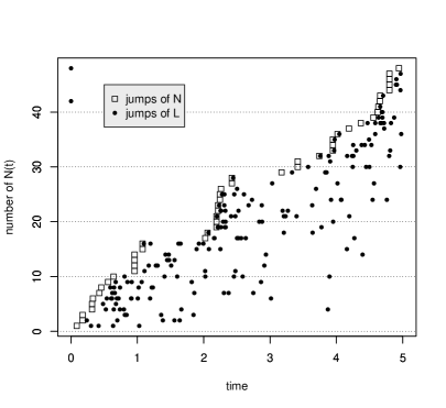
Figure 1. Left: we present the model $M(t),\,t\in[0,5]$ of (1.1) with $L$ to be a non-homogeneous Poisson, where processes $N$ and $(L_{j})$ are plotted separately. Dots by $\square$ denote jumps $(T_{j})$ of $N$ and dots by $\bullet$ on the same $y$-coordinate as that of $T_{j}$ are the corresponding jumps by $L(t-T_{j})$. The dots $\bullet$ on the $y$-axis suggest that no jumps by the stream $L(t-T_{j})$ are observed for these $j$’s on $[0,5]$. Right: we examine the predictors of $M(t),\,t\in[0,5]$ for different intervals. Dots $\bullet$ imply the real observation of $M(t),\,t\in[0,5]$, while sequences of dots $\square\sim+$ respectively denote predictors ${\mathbb{E}}[M(s,5]\mid\mathcal{G}_{s}],\,s=1,2,\ldots,4$.

References

- [1] Barndorff-Nielsen, O. E. and Shiryaev, A. (2010) Change of Time and Change of Measure. Vol. 13. World Scientific Publishing, Singapore.
- [2] Bochner, S. (2005) Harmonic Analysis and the Theory of Probability. Dover Publications, New York.
- [3] Bondesson, L. (2006), Shot-Noise Processes and Distributions. Encyclopedia of Statistical Sciences, John Wiley & Sons, Inc.
- [4] Chung, K.L. (2001) A Course in Probability Theory. 3rd ed. Academic Press, London.
- [5] Embrechts, P., Klüppelberg, C. and Mikosch, T. (1997) Modelling Extremal Events for Insurance and Finance. Springer, Berlin.
- [6] Faÿ, G., González-Arévalo, B., Mikosch, T. and Samorodnitsky, G. (2006) Modeling teletraffic arrivals by a Poisson cluster process. Queueing Syst. 54, 121–140.
- [7] Grandell, J. (1997) Mixed Poisson Processes. Chapman and Hall/CRC, London.
- [8] Grauert, H. and Fritzsche, K. (1976) Several Complex Variables. Springer, New York.
- [9] Kallenberg, O. (1983) Random Measures. 3rd ed. Academic Press, London.
- [10] Kallenberg, O. (2002) Foundations of Modern Probability. 2nd ed. Springer, New York.
- [11] Klüppelberg, C. and Kühn, C. (2004) Fractional Brownian motion as a weak limit of Poisson shot noise processes—with applications to finance. Stochastic Process. Appl. 113, 333–351.
- [12] Klüppelberg, C. and Matsui, M. (2015) Generalized fractional Lévy processes with fractional Brownian motion limit. Adv. in Appl. Probab. 47, 1108–1131.
- [13] Lund, R.B., Butler, R.W. and Paige, R.L. (1999) Prediction of shot noise. J. Appl. Probab. 36, 374–388.
- [14] Matsui, M. (2017) Prediction of components in random sums. Methodol. Comput. Appl. Probab. 19, 573–587.
- [15] Matsui, M. and Mikosch, T. (2010) Prediction in a Poisson cluster model. J. Appl. Probab. 47, 350–366.
- [16] Matsui, M. and Rolski, T. (2016) Prediction in a mixed Poisson cluster model. Stoch. Models. 32, 460–480.
- [17] Matthes, K., Kerstan, J. and Mecke, J. (1978) Infinitely Divisible Point Processes. Wiley, New York.
- [18] Mikosch, T. (2009) Non-Life Insurance Mathematics. An Introduction with the Poisson Process. 2nd ed. Springer, Heidelberg.
- [19] Mikosch, T. and Samorodnitsky, G. (2007) Scaling limits for cumulative input processes. Math. Oper. Res. 32, 890–918.
- [20] Norberg, R. (1993) Prediction of outstanding liabilities in non-life insurance. Astin Bull. 23, 95–115.
- [21] Norberg, R. (1999) Prediction of outstanding liabilities II. Model variations and extensions. Astin Bull. 29, 5–25.
- [22] Rajput, B. S. and Rosinski, J. (1989). Spectral representations of infinitely divisible processes. Probab. Theory Related Fields 82, 451–487.
- [23] Reiss, R.-D. (1989) Approximate Distributions of Order Statistics. Springer, New York.
- [24] Rolski, T., Schmidli, H., Schmidt, V. and Teugels, J. (1999) Stochastic Processes for Insurance and Finance, Wiley, West Sussex.
- [25] Rolski, T. and Tomanek, A. (2011) Asymptotics of conditional moments of the summand in Poisson compounds. J. Appl. Probab. 48A, 65–76.
- [26] Rolski, T. and Tomanek, A. (2014) A continuous-time model for claims reserving. Applicationes Mathematicae 41, 277–300.
- [27] Sato, K. (1999) Lévy Processes and Infinitely Divisible Distributions. Cambridge University Press, Cambridge.
- [28] Schmidt, T. (2017) Shot-Noise Processes in Finance. Forthcoming in From Statistics to Mathematical Finance the Festschrift in honor of Winfried Stute, Springer.