Prospects for Measuring Planetary Spin and Frame-Dragging
in Spacecraft Timing Signals

Abstract

Satellite tracking involves sending electromagnetic signals to Earth. Both the orbit of the spacecraft and the electromagnetic signals themselves are affected by the curvature of spacetime. The arrival time of the pulses is compared to the ticks of local clocks to reconstruct the orbital path of the satellite to high accuracy, and to implicitly measure general relativistic effects. In particular, Schwarzschild space curvature (static) and frame-dragging (stationary) due to the planet’s spin affect the satellite’s orbit. The dominant relativistic effect on the path of the signal photons is Shapiro delay due to static space curvature. We compute these effects for some current and proposed space missions, using a Hamiltonian formulation in four dimensions. For highly eccentric orbits, such as in the Juno mission and in the Cassini Grand Finale, the relativistic effects have a kick-like nature, which could be advantageous for detecting them if their signatures are properly modeled as functions of time. Frame-dragging appears, in principle, measurable by Juno and Cassini, though not by Galileo $5$ and $6$. Practical measurement would require disentangling frame-dragging from the Newtonian “foreground” such as the gravitational quadrupole which has an impact on both the spacecraft’s orbit and the signal propagation. The foreground problem remains to be solved.

I Introduction

General relativity (GR) describes gravitation as a consequence of a curved four dimensional spacetime Iorio (2015); Debono and Smoot (2016). In most astrophysical systems, however, dynamics are dominated by Newtonian physics and GR only provides very small perturbations. Near a mass $M$, the relativistic perturbations on an orbiting or passing body depend mostly on the pericenter distance, which we call $p$, in units of the gravitational radius $GM/c^{2}$. Newtonian effects are of order $O(p^{-1/2})$. The largest relativistic perturbation is time dilation, and is of $O(p^{-1})$. Space curvature, referring to space-space terms in the metric tensor, enters dynamics at $O(p^{-3/2})$. At $O(p^{-2})$ mixed space-time metric terms enter the dynamics; these correspond to frame-dragging effects, in which a spinning mass drags spacetime in its vicinity and thereby affects the orbit and orientation of objects in its gravitational field. Gravitational radiation corresponds to dynamical effects of $O(p^{-3})$. In post-Newtonian notation, X PN (e.g. $1$ PN, $2$ PN, …) corresponds to $O(p^{-{\rm X}-1/2})$. In the Solar System, $p$ is very large in gravitational terms: $\sim 10^{8}$ or more. In close binary systems $p$ can be much less. In binary pulsars the combination of comparatively low $p\sim 10^{5}$ with the long-term stability of pulsar timing enables the measurement of relativistic effects down to gravitational radiationTaylor (1994); Kramer et al. (2006).

All the same effects are, in principle, present for artificial Earth satellites, but since $p\sim 10^{9}$, they are much weaker. Nonetheless, until now the frame-dragging effect of the Earth’s spin has been detected in two different ways: (1) the LAGEOS and LARES satellites used laser ranging to measure orbital perturbations from frame-dragging Ciufolini and Pavlis (2004); Ciufolini et al. (2016) (some aspects are still controversial Iorio et al. (2011); Renzetti (2013, 2015); Iorio (2017)); (2) Gravity Probe B measured the effects of frame-dragging on the orientation of onboard gyroscopes Everitt et al. (2011). GPS satellites are well known to be sensitive to time dilation Ashby (2003) and upcoming missions will put even more precise clocks in orbit. In the Atomic Clock Ensemble in Space (ACES) mission Cacciapuoti and Salomon (2011), two atomic clocks will be brought to the ISS in order to perform such experiments. However, the ISS is not the optimal place to probe GR and a dedicated satellite on a highly eccentric orbit would be desirable. Its proximity to Earth and high velocity at pericenter would boost relativistic effects and therefore improve the measurements. Several such satellites equipped with an onboard atomic clock and a microwave or optical link on very eccentric orbits, such as STE-QUEST, have been discussed and studied Altschul, B. et al. (2015). Such missions would not only be very interesting to probe gravity but also have a plethora of applications, e.g., in geophysics Bondarescu et al. (2012, 2015).

Missions like Juno and Cassini present new possibilities for measuring relativistic effects around the giant planets in our Solar System. The basic idea goes back to the early days of general relativity, when Lense and Thirring Lense and Thirring (1918) showed that the orbital plane of a satellite precesses about the spin axis of the planet —that is what we now call frame-dragging— and identified the expected precession of Amalthea’s orbit by $1^{\prime}\,53^{\prime\prime}$ per century as the most interesting case. Recent work has drawn attention to the corresponding precession in the case of Juno Helled et al. (2011); Iorio (2013, 2010) and other systems Iorio (2011, 2012); Iorio, L. (2005).

The classical Lense-Thirring precession is an orbit-averaged effect. This comes with the problem that the very small precession due to relativity is masked by much larger non-relativistic precession, making it very hard to identify the relativistic contribution. For example, most of Mercury’s observed precession is due to Newtonian planetary perturbations, the relativistic contribution being only about $7\%$ of the total Park et al. (2017). It is better to have something with a specific time dependence that can be filtered out.

Here, we extend the work of Angelil et al. for terrestrial satellites Angélil et al. (2014) and the Galactic center Kannan and Saha (2009); Preto and Saha (2009); Angélil and Saha (2010); Angélil et al. (2010); Angélil and Saha (2011, 2014); Zhang and Iorio (2017) and apply it to other planets in the Solar System. Since the orbits are dominated by Newtonian physics, and relativity only contributes very small perturbations, their investigation is numerically challenging. In earlier work Angélil et al. (2014) the orbits were therefore simulated with smaller semi-major axes compared to the real orbit and then, by knowing how the individual effects scale, the redshift curves were obtained by correctly scaling up. Here, we use an arbitrary precision code instead.

We look at an idealized model where a spacecraft sends electromagnetic signals to a ground station. Comparing the relativistic $4$-momentum of the emitted photon to that of the one received at the station allows determining a redshift $z$ (see Eq. (3)). Equivalently, one can consider an orbiting clock which sends out signals corresponding to the ticks of the clock Angélil and Saha (2010); Angélil et al. (2014). Then, the redshift arises when two photons emitted by the spacecraft at an interval of proper time $\Delta\tau$ travel through curved spacetime hitting the observer with a difference in the arrival time $\Delta t=\Delta\tau(1+z)$. In both cases, a one-way signal transfer is considered. Typically, satellite communication systems allow two-way signal transfer. For a comparison of distant ground clocks like done with ACES, this leads to a first order cancellation of the position errors of the clocks Duchayne, L. et al. (2009).

To estimate the relativistic effects, we solve for the trajectory of

1. the satellite in a curved spacetime, and

2. the photons (or propagating ticks from the frequency standard) as they propagate to the receiving station

in a given gravitational field. Both the satellite and the photons follow geodesics of the metric and can be obtained by integrating the relativistic Hamiltonian, expanded in velocity orders. The redshift depends on both the classical Doppler shift as well as a number of relativistic effects. Both trajectories are generated numerically via a simulation code that handles multiple scales through variable precision. The effects are modulated by the varying gravitational field.

The paper proceeds as follows: Sec. II describes the approximations we make for the spacetime outside a planet. It presents the Hamiltonian system that is being solved numerically with the higher order relativistic effects, and their respective scalings with orbital size. We then compute the magnitude of the spin parameter, of Schwarzschild precession and frame-dragging effects for the planets in our Solar System, and report them relative to the effects around Earth for orbits of similar proportionality. Sec. IV A and B apply this formalism to the Juno and Cassini Missions. Sec. IV C discusses the Galileo 5 and 6 satellites and other proposed Earth-bound missions. In particular, it discusses the importance of eccentricity in detecting relativistic effects.

Conclusions and potential future directions are presented in Sec. V.

II General Relativistic effects

Calculating relativistic effects fundamentally involves two things: the metric and the geodesic equations. The well-known epigram by J.A. Wheeler states Spacetime tells matter how to move, matter tells spacetime how to curve. The metric is known explicitly in terms of the masses, including mass multipoles, and spin rates. The geodesic equation, in general, requires a numerical solution. However, in special or approximate cases analytical solutions also exist Klioner and Kopeikin (1992); Ashby and Bertotti (2010); Hees et al. (2014); Crosta et al. (2015); D’Orazio and Saha (2010).

We wish to understand how different terms in the metric, in particular the spin part, affect the observable redshift signal. To do this, we will numerically integrate the geodesic equations with different metric terms turned on and off and compare the resulting redshift signal curves.

In Sec. II.1 we briefly introduce the Hamiltonian formalism and the formula for calculating the redshift. This is followed by Sec. II.2, which discusses the expansion of both the orbital as well as the signal Hamiltonian. In Sec. II.3 we discuss the spin parameter and in II.4 we discuss the cumulative changes of the Keplerian elements due to orbital relativistic effects. Finally, in Sec. II.5 we investigate how the sizes of the relativistic signals scale for the different planets in the Solar System.

II.1 Basic formulation

We work with the geodesic equations in four dimensions, in Hamiltonian form. The independent variable is not time, but the affine parameter, which is just the proper time in arbitrary units. Although the formalism seems complex, it actually tends to lead to simpler equations Angélil and Saha (2010); Angélil et al. (2014) than other formulations.

For any spacetime metric, the geodesic equations may be expressed in Hamiltonian form as

$$\frac{dx^{\mu}}{d\lambda}=\frac{\partial H}{\partial p_{\mu}}\qquad\frac{dp_{\mu}}{d\lambda}=-\frac{\partial H}{\partial x^{\mu}}$$ (1)

where

$$H={\textstyle\frac{1}{2}}g^{\mu\nu}(x^{\alpha})p_{\mu}p_{\nu}$$ (2)

with $x^{\mu}=(t,r^{i})$ being the four-dimensional coordinates, $p_{\mu}=(p_{t},p_{i})$ being the canonical momenta, and $\lambda$ being the affine parameter.

The satellite at position $\vec{r}=(r^{i})$ orbiting with 4-velocity $u^{\mu}_{\text{emit}}$ emits a photon with 4-momentum $p_{\mu}^{\text{emit}}$ which arrives at an observer (having velocity $u^{\nu}_{\text{obs}}$) with momentum $p_{\nu}^{\text{obs}}$. The redshift is then given by

$$z=\frac{p_{\mu}^{\text{emit}}u^{\mu}_{\text{emit}}}{p_{\nu}^{\text{obs}}u^{\nu}_{\text{obs}}}-1.$$ (3)

For a distant observer at rest, the redshift for orbital effects reduces to

$$z=\frac{1}{c}u^{t}_{\text{emit}}-\frac{1}{c}u^{\text{LOS}}_{\text{emit}}-1,$$ (4)

where $u^{\text{LOS}}_{\text{emit}}$ is the satellite’s velocity along the line of sight.

II.2 The expanded Hamiltonian

In this subsection we use geometrized units. That is, $\vec{r}$ is measured in units of $GM/c^{2}$ where $M$ is the planetary mass, while $t$ is measured in units of $GM/c^{3}$. The momentum is dimensionless. Since the orbits considered are close to Keplerian, the order-of-magnitude relations

$$|\vec{p}|\sim\frac{v}{c},\qquad r\sim\left(\frac{v}{c}\right)^{-2}$$ (5)

will hold, where $v$ is the orbital speed. The time-momentum $p_{t}$ is constant and its value only affects internal units of a calculation. It is convenient to set $p_{t}=-1$.

As usual in post-Newtonian celestial mechanics, we order contributions in powers of $v/c$. These correspond to different physical effects. Moreover, the ordering in powers of $v/c$ is different for the spacecraft orbit and the light signals. Accordingly, we consider two Hamiltonians, as follows.

$$H^{\text{orbit}} =H^{\text{equiv-prin}}+H^{\text{Schwarzschild}}+H^{\text{spin}}$$ (6)

$$H^{\text{signal}} =H^{\text{Minkowski}}+H^{\text{Shapiro}}$$

Since there is only one spacetime, $H^{\text{orbit}}$ and $H^{\text{signal}}$ are just different approximations to the same underlying Hamiltonian.

The orbit of the satellite is dominated by

$$H^{\text{equiv-prin}}=-\frac{p_{t}^{2}}{2}+\left(-p_{t}^{2}\,U(\vec{r}\,)+\frac{{\vec{p}\,}^{2}}{2}\right)$$ (7)

where $U(\vec{r})$ is minus the Newtonian gravitational potential, to leading order $1/r$ but also including multipole moments $J_{n}$ as well as the tidal potential due to the Sun and other planets. The first term on the right is of order unity, while the bracketed part is of order $v^{2}/c^{2}$. This Hamiltonian leads to a Newtonian orbit and redshift contribution of order $v/c$, together with a time dilation effect of order $v^{2}/c^{2}$. Gravitational time dilation is a basic consequence of the geometric description of spacetime, i.e., the principle of equivalence. Indeed, equation (7) is the simplest Hamiltonian consistent with the equivalence principle that gives the correct Newtonian limit. Moving clocks tick slower than stationary ones. So do clocks in a gravitational field. For an orbiting clock, both effects are equal to leading order. The ground station will have its own time dilation too, of course, and the difference is what matters. Time dilation causes the localization of a satellite to be off by kilometers, which has already been taken into account by the early phases of GPS. While this relativistic effect is well established, the Galileo satellites will measure it to unprecedented precision.

Since higher order relativistic effects cause small changes in the redshift, they can be studied perturbatively. We investigate each effect individually by adding it to $H^{\text{equiv-prin}}$, and computing the cumulative redshift. The redshift perturbation is obtained by subtracting the redshift when the effect is artificially turned off.

The next contribution to $H^{\text{orbit}}$ is

$$H^{\text{Schwarzschild}}=-\frac{p_{t}^{2}}{r^{2}}-\frac{{\vec{p}\,}^{2}}{r}$$ (8)

which introduces the effect of space curvature in the Schwarzschild spacetime. It is easy to verify from equation (5) that the Hamiltonian terms are of order $s\,v^{4}/c^{4}$, and they contribute to redshift at order $s\,v^{3}/c^{3}$, where $s$ is the spin parameter. Note that the $s$ is larger for planets ($\sim 10^{2}-10^{3}$) than for more compact systems like black holes ($s\sim 1$) and thus the spin terms are significantly larger than what one would expect from just looking at velocity order.

The leading-order frame-dragging effect arises when adding the term

$$H^{\text{spin}}=-\frac{2p_{t}}{r^{3}}\,\vec{p}\cdot(\vec{s}\times\vec{r}).$$ (9)

This term is of order $s\,v^{5}/c^{5}$ and contributes a redshift effect of order $s\,v^{4}/c^{4}$. Frame-dragging is due to the rotation of the central mass, which spins with $\vec{s}$, and depends linearly on the spin parameter $s=|\vec{s}|$. At next higher order, the dominant term is a spin-squared term, i.e., it is proportional to $s^{2}$ Angélil et al. (2014). This effect has never been measured before. But since $s$ is quite large for planets (see Table 1), probing this effect should be within the scope of future satellite missions.

The leading multipole contribution comes from $J_{2}$ in the Newtonian Hamiltonian (7) and scales as $1/r^{3}$. Therefore, it has a different $r$-dependence as the relativistic effects discussed here. The relativistic effect with the same $r$-scaling would be the spin-squared effect.

The main contribution to the redshift comes from the velocity along the line of sight. Therefore, in order to measure a certain relativistic effect, it is desirable to have an orbit-observer-configuration where the relativistic effect has a significant contribution to the line of sight velocity. For first order spin, the leading contribution is given by

$$\Delta z_{\text{spin}}=-\frac{2}{r^{2}}\vec{s}\cdot(\hat{r}\times\hat{b}),$$ (10)

where $\hat{b}$ is the unit vector pointing from the satellite towards the observer. Interestingly, the spin related redshift contribution has no explicit dependence on the satellite’s velocity.

The signal photons travel to leading order on a straight line. The leading relativistic effect, leading to a slight bending, is Shapiro delay. This part is best analyzed after transforming to a Solar System frame. The signal Hamiltonian is given by the sum of

$$H^{\text{Minkowski}}=-\frac{p_{t}^{2}}{2}+\frac{{\vec{p}\,}^{2}}{2}$$ (11)

and

$$H^{\text{Shapiro}}=-U({\vec{p}}\,)\left(p_{t}^{2}+{\vec{p}\,}^{2}\right)\,.$$ (12)

At the next order of expansion, further Shapiro-like terms as well as spin terms appear. However, they are expected to be too small to be measured. The effect of frame-dragging on light signals was calculated, e.g., by Kopeikin (1997); Wex and Kopeikin (1999).

II.3 The spin parameter

The dimensionless spin parameter of a celestial body is given by

$$s=\frac{c}{GM^{2}}\int\rho(\vec{x})\,\omega(\vec{x})\,r_{\perp}^{2}\,d^{3}\vec{x}\,.$$ (13)

For solid-body rotation ($\omega=2\pi/P$, where $P$ is the spin period) the above expression reduces to

$$s=2\pi\times\hbox{MoI}\times\frac{c}{gP}$$ (14)

where

$$\hbox{MoI}=\frac{1}{MR^{2}}\int\rho(\vec{x})\,r_{\perp}^{2}\,d^{3}\vec{x}$$ (15)

is the dimensionless moment of inertia and $g=GM/R^{2}$ is the surface gravity, where $R$ is the average radius of the body. For realistic density and $\omega$ profiles

$$s\sim\frac{c}{gP}$$ (16)

is still a useful rough estimate. It may be convenient to remember it as the number of days needed to reach the speed of light from an acceleration of one $g$.

For yet another interpretation of the spin parameter, let us consider two speeds: the surface speed of a spinning planet $v_{s}\sim R/P$ and the launching speed needed to send something into orbit from the surface $v_{l}^{2}\sim gR$. In terms of these speeds, the approximate formula (16) becomes

$$s\sim\frac{cv_{s}}{v_{l}^{2}}\raise 2.15277pt\hbox{.}$$ (17)

The maximal-spinning situation $v_{s}\approx v_{l}$ corresponds to a planet spinning so fast that it almost breaks up under centrifugal forces. In this limit $s\sim c/v_{l}$. Recalling the orders in $H^{\text{spin}}$ in equation (9), we can see that that Hamiltonian term would be of order $v^{4}/c^{4}$ and the corresponding redshift effect would be of order $v^{3}/c^{3}$. That is, for a low-orbiting spacecraft above a maximally-spinning planet, relativistic spin effects will be comparable in size to space-curvature effects.

II.4 Keplerian elements

A Keplerian orbit is described by the Keplerian elements $a,e,\Omega,I$ and $\omega$. While $a$ and $e$ describe the size and the eccentricity of the ellipse, the three angles describe its orientation with respect to some reference plane.

For a relativistic orbit this is not true anymore, as the relativistic effects induce deviations from Keplerian motion. In principle, however, it is still possible to determine the instantaneous Keplerian elements at each point along the orbit: These correspond to a Keplerian orbit having exactly the same velocity as the relativistic one at a given position.

It is well-known that space curvature leads to a precession of the pericenter

$$\Delta\omega_{\text{SS}}=\frac{GM}{c^{2}}\frac{6\pi}{a(1-e^{2})}$$ (18)

for one orbit.

However, $\omega$ is not shifted evenly along the orbit, in fact, there is almost no shift during most of the orbit, but around pericenter there is a kick-like shift. Similarly, there is a precession of the pericenter due to frame-dragging Lense and Thirring (1918); Mashhoon et al. (1984)

$$\Delta\omega_{\text{Spin1}}=-s\frac{12\pi\sqrt{GM}\cos I}{\left[a(1-e^{2})\right]^{3/2}}$$ (19)

per orbit and also there is a precession of the longitude of the ascending node

$$\Delta\Omega_{\text{Spin1}}=s\frac{4\pi\sqrt{GM}}{\left[a(1-e^{2})\right]^{3/2}}$$ (20)

per orbit. Fig. 1 shows the precession of the longitude of the ascending node together with the actual shift for a typical Juno orbit.

Measuring time-averaged precessions is not actually a useful strategy, because the slightest use of spacecraft engines changes all the Keplerian elements. But similarly to the Keplerian elements, relativistic effects affect the observed redshift in a kick-like manner at pericenter. Therefore, relativistic effects influence a single pericenter passage and when the instrument is accurate enough, they can be probed as a function of time vs. waiting for their build up over many orbits.

II.5 Scaling of relativistic effects

The size of the effects scale with the size of the orbit Angélil and Saha (2010). For Schwarzschild space curvature and first order spin, the respective scaling laws for the residual redshifts are $\Delta z^{\text{SS}}\sim(r_{G}/r)^{3/2}$ and $\Delta z^{\text{Spin1}}\sim s(r_{G}/r)^{2}$ where $r_{G}=GM/c^{2}$ is the gravitational radius. Writing distances in terms of planetary radii $r=\alpha R$, we obtain

$$\frac{\Delta z_{1}}{\Delta z_{2}}=\left(\frac{s_{1}}{s_{2}}\right)^{m}\left(\frac{r_{G}^{1}}{r_{G}^{2}}\frac{r_{2}}{r_{1}}\right)^{n}=\left(\frac{s_{1}}{s_{2}}\right)^{m}\left(\frac{U_{1}}{U_{2}}\frac{\alpha_{2}}{\alpha_{1}}\right)^{n},$$ (21)

where $U_{i}=GM_{i}/(R_{i}c^{2})$ is the gravitational potential at the surface of planet $i$ and $m=0,1$ and $n=3/2,2$ for Schwarzschild curvature and first order spin effect, respectively. For similar orbits around different planets, i.e., $\alpha_{1}=\alpha_{2}$ with the same eccentricity and identical Keplerian angles, this reduces to $\Delta z_{1}/\Delta z_{2}=(s_{1}/s_{2})^{m}(U_{1}/U_{2})^{n}$. Thus, the higher the compactness $M/R$ of a planet, the higher the relativistic effect. For frame-dragging effects, the spin parameter has also to be taken into account.

Using the expression above, we can compare the sizes of relativistic effects of orbits around the planets, the Moon and the Sun to terrestrial orbits. The ratio between the signals for similar orbits is given in Table 1.

III Planetary parameters

The planetary parameters relevant for calculating relativistic effects are summarised in Table 1. The Moon and the Sun are also included for comparison.

The values of the gravitational potential $U$ at the surface are ordered as one might expect. Jupiter with $2\times 10^{-8}$ has the highest, while for the Earth the value is 30 times smaller.

The values of the spin parameter may be surprising. Black holes must have $s<1$ as is well known, but planets can have $s\gg 1$. Mars has the highest $s\sim 2090$, while Venus has the lowest $s\sim 3$, but most planets have an $s$ with a value that is typically in the hundreds. Incidentally, the Sun’s spin parameter will be small: The Sun has a much larger $g$ than any planet, and it spins differentially, roughly once a month; as a result, the Sun has a much smaller $s$ than the Earth. The uncertainty in $s$ depends on the uncertainties in the MoI and in the spin period.

Although neither the density profile nor internal differential rotation can be measured directly, internal structure models provide MoI values for the gas giants, and these are thought to be accurate to a few percent Helled (2011); Helled et al. (2011); Nettelmann et al. (2015). The Radau-Darwin approximation Zharkov and Trubitsyn (1980) relates the MoI to the gravitational quadrupole $J_{2}$ and the ratio of centrifugal to gravitational acceleration at the equator. In future it may become possible to measure planetary MOI from precession Maistre et al. (2016). At present, the estimated MoI is $\sim 0.265$ for Jupiter Helled et al. (2011) and $\sim 0.220$ for Saturn Guillot and Gautier (2007); Helled (2011). Evidently, Saturn is more centrally condensed than Jupiter.

The rotation period remains somewhat uncertain for all the giant planets other than Jupiter Helled et al. (2010, 2009, 2015). Saturn’s internal rotation period is unknown to within $\sim 10$ minutes. It has been acknowledged that the rotation period is unknown since Cassini ’s Saturn kilometric radiation (SKR) measured a rotation period of 10h 47m 6s Gurnett et al. (2007), longer by about eight minutes than the radio period of 10h 39m 22.4s measured by Voyager Ingersoll and Pollard (1982). In addition, during Cassini ’s orbit around Saturn the radio period was found to be changing with time. It then became clear that SKR measurements do not represent the rotation period of Saturn’s deep interior. Due to the alignment of the magnetic pole with the rotation axis, Saturn’s rotation period cannot be obtained from magnetic field measurements Sterenborg and Bloxham (2010). Theoretical efforts to infer the rotation period Anderson and Schubert (2007); Read et al. (2009); Helled et al. (2015) indicate further sources of uncertainty. Saturn’s rotation period is thought to be between $\sim$ 10h 32m and $\sim$ 10h 47m. For Uranus and Neptune, the uncertainty could be as large as 4% and 8%, respectively Helled et al. (2010).

A further complexity arises from the fact that the giant planets could have non-body rotations (e.g., differential rotation on cylinders/spheres) and/or deep winds. However, in that case, the deviation from a mean solid-body rotation period is expected to be small. Future space missions to Uranus and/or Neptune, performing accurate measurements of their gravitational fields, could be used to determine the spin parameter of these planets.

Object	$U\equiv GM/(c^{2}R)$	$g\equiv GM/R^{2}$ $[m/s^{2}]$	MoI	$s$	spin period [days]	$\frac{\Delta z_{\text{SS,Obj}}}{\Delta z_{\text{SS,Earth}}}$	$\frac{\Delta z_{\text{Spin,Obj}}}{\Delta z_{\text{Spin,Earth}}}$
Mercury	$1.00\times 10^{-10}$	3.7	$0.35$	$35.2$	58.65	$5.5\times 10^{-2}$	$9.9\times 10^{-4}$
Venus	$5.98\times 10^{-10}$	8.9	$0.33$	$3.3$	243.02	$8.0\times 10^{-1}$	$3.3\times 10^{-3}$
Earth	$6.95\times 10^{-10}$	9.8	$0.3308$	$738.3$	1.00	$1.0$	$1.0$
Moon	$3.12\times 10^{-11}$	1.6	$0.394$	$194.8$	27.32	$9.5\times 10^{-3}$	$5.3\times 10^{-4}$
Mars	$1.40\times 10^{-10}$	3.7	$0.366$	$2093.5$	1.02	$9.1\times 10^{-2}$	$1.2\times 10^{-1}$
Jupiter	$2.02\times 10^{-8}$	25.9	$0.265$	$564.0$	0.41	$1.6\times 10^{2}$	$6.4\times 10^{2}$
Saturn	$7.00\times 10^{-9}$	10.4	$0.220$	$988.0$	0.44–0.45	$3.2\times 10^{1}$	$1.4\times 10^{2}$
Uranus	$2.52\times 10^{-9}$	8.9	$0.225$	$770.1$	0.67–0.76	$6.9$	$1.4\times 10^{1}$
Neptune	$3.06\times 10^{-9}$	11.1	0.236	691	0.63–0.71	$9.2$	$1.8\times 10^{1}$
Sun	$2.12\times 10^{-6}$	273.7	$0.07$	$0.2$	25.05	$1.7\times 10^{5}$	$2.8\times 10^{3}$

Table 1: Gravitational and spin parameters for the planets and the Moon. For the gravitational potential $U$ and acceleration $g$, values at the surface are given; values from orbit will be somewhat smaller. MoI values for the giant planets are derived using interior models that reproduce the gravitational fields of the planets Helled et al. (2015). All other quantities are derived using parameters provided by NASA [http://nssdc.gsfc.nasa.gov/planetary/factsheet]. The two columns on the right give the ratio between the redshift signals of orbits around the respective object and the signals for a similar orbit around Earth.

IV Relativistic effects for Current and Planned Missions

We now determine the effects of relativity on the redshift signal for different orbits around different planets. In Sec. IV.1 we consider a typical orbit of the Juno spacecraft around Jupiter, followed by a typical Cassini orbit around Saturn in Sec. IV.2. Finally, in Sec. IV.3, we discuss terrestrial orbits.

IV.1 Jupiter orbit

On July 4, 2016, the Juno mission arrived at Jupiter and started orbiting the planet. It is equipped to perform high precision measurements (operating at X-band and Ka-band) of its gravitational field. The $53$-days orbits are polar with perijove being at $\sim 1.09$ Jupiter radii and apojove at $\sim 120$ Jupiter radii. Such orbits provide ideal conditions for gravitational field measurements, and allow the spacecraft to avoid most of the Jovian radiation field. After more than four years of measurementes and $\sim 32$ orbits around Jupiter, Juno is planned to make one last orbit and then perform the deorbiting maneuver (see e.g., Matousek (2007)).

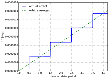
Figure 1: Change of the longitude of the ascending node $\Omega$ for a typical Juno orbit due to spin. The solid line shows the actual change of $\Omega$, while the dashed line represents the averaged change given by Eq. (20).

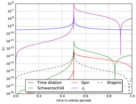
Figure 2: Higher order relativistic effects for the Juno orbiter. The plot shows the magnitude of the redshift signal due to the different relativistic effects. The parameters chosen correspond to a typical science orbit. The curves change slightly for other orbits, however, the order of magnitude of the effects is the same. Also the Newtonian effect due to $J_{2}$ is shown.

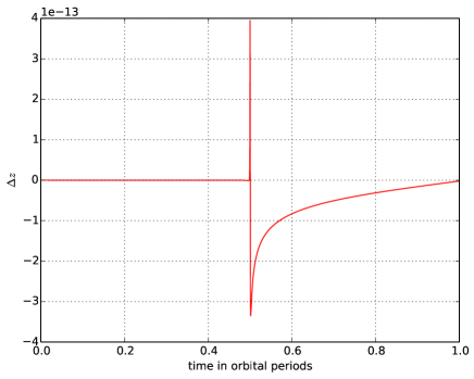
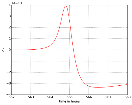
Figure 3: Upper: contribution to the redshift from frame-dragging by Jupiter’s spin, for the same orbit as in Fig. 2. The signal peaks at the orbit pericenter passage. Lower: zoom into pericenter passage.

We compute the leading-order relativistic effects on the orbit of the Juno mission. They measure the precession of the orbit due to the curvature of the spacetime and contain a part that accumulates as well as a transient part, which has never been measured. The effect that occurs due to the Schwarzschild term in the Hamiltonian produces a Mercury-like precession (solid red curve), while the other is referred to as frame-dragging due to the spin of Jupiter. Measuring the latter directly constrains the spin parameter of the planet, which is proportional to its moment of inertial and angular momentum. It thus reveals important information about the planet’s internal density structure that is not necessarily identical to that contained in the gravitational moments.

The Juno orbiter has already entered a highly elliptical polar orbit around Jupiter. It is measuring deviations in the velocity of the spacecraft $\sim 10\mu m$/sec $(\tau/60$ sec $)^{-1/2}$. This corresponds to a sensitivity to redshift change of $\Delta z\sim 3\times 10^{-14}$.

At each pericenter passage of Juno, both the instantaneous Keplerian elements and the orientation to the observer change. Therefore, in order to discuss relativistic effects on the basis of the Juno mission, we consider a typical orbit with average values $a=60\times R_{\text{Jupiter}}$, $e=0.981$, $\Omega=253^{\circ}$, $I=93.3^{\circ}$, $\omega=170^{\circ}$ and observer position $\theta_{\text{obs}}=92.9^{\circ}$ (polar angle), $\phi_{\text{obs}}=15.0^{\circ}$ (azimuthal angle). Fig. 2 shows the characteristic redshift curves for the different effects for such a Juno orbit. For all science orbits, the sizes of the effects, in particular of the spin effect, are similar.

Fig. 3 shows the part in the redshift due to the presence of Jupiter’s spin over one orbit. After pericenter passage, the relativistic and the non-relativistic orbit are out of sync and a comparison does not make sense anymore. The lower panel of the figure zooms into the peak around pericenter, revealing that the interesting time span is of order $\sim 1$ hour. This is the phase that needs to be observed in order to seek the characteristic imprint of frame-dragging in the redshift data.

Over any one orbit, only one component of the spin vector contributes at leading order, namely the spin component along $\hat{r}_{\rm peri}\times\hat{b}$ (see Eq. 10). To be sensitive to all components of the spin, orbits with different orientations of $\hat{r}_{\rm peri}\times\hat{b}$ are needed. Fig. 4 shows the polar and azimuthal angles of this vector for all the Juno science orbits. The orientations are varied, and hence Juno is sensitive to all three components of the spin vector.

The frame-dragging effect will, moreover, be a pathfinder to measuring yet weaker effects. The spin terms depend on the spin profile inside the planet. Measuring the spin profile would therefore play a role in constraining planet properties and formation models. Future deep-space missions could enable tests of general relativity around other planets in the Solar System whose composition and internal structure are unknown.

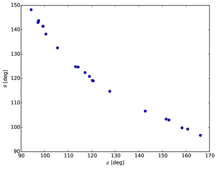
Figure 4: Orientation of the vector $\hat{r}_{\rm peri}\times\hat{b}$ for Juno science orbits. Here $\hat{b}$ is the line of sight to Juno, and $\theta,\phi$ in the Figure are with respect to to Jupiter’s axis. The timing signal is sensitive to the planetary spin projected along these various directions.

IV.2 Saturn orbit

The Cassini mission is planned to finish its exploration of the Saturnian system with proximal orbits around Saturn that will provide accurate measurements of the gravitational field of the planet. The Cassini spacecraft is planned to execute $22$ highly inclined ($63.4$ degree) orbits with a periapsis of $\sim 1.02$ Saturn radii Edgington and Spilker (2016). These proximal orbits, known as Cassini Grand Finale, operating at X-band, are also ideal for gravity measurements. They are expected to provide range rate accuracies of $\sim 12\mu{\rm m/sec}$ at 1000 second integration times, being about four times noisier than Juno.

Both the Juno and the Cassini spacecrafts will terminate their operations by descending into the atmospheres of Jupiter and Saturn, respectively, and will disintegrate and burn up in order to fulfill the requirements of NASA’s Planetary Protection Guidelines.

Cassini has a sensitivity that is about $\Delta z\sim 10^{-13}$. Relativistic effects peak around the pericenter with the frame-dragging effect of maximum amplitude $\sim 10^{-13}$ and the Schwarzschild curvature term of $\sim 10^{-11}$. Ideally, the goal would be to resolve both the Schwarzschild and frame-dragging parts of the precession as a function of time. If they could be modeled effectively, they would less likely be drowned by Newtonian noise than a cumulative effect.

Fig. 5 shows the corresponding curves for a typical Cassini orbit. For Cassini, we chose the values $a=10\times R_{\text{Saturn}}$, $e=0.9$, $\Omega=175^{\circ}$, $I=62^{\circ}$, $\omega=187^{\circ}$, $\theta_{\text{obs}}=63.3^{\circ}$ and $\phi_{\text{obs}}=-5^{\circ}$.

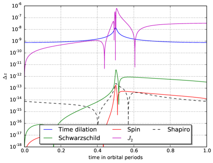
Figure 5: Higher order relativistic effects for Cassini.

IV.3 Earth orbit

Next we discuss satellites in Earth orbit. To illustrate the importance of eccentricity, Fig. 6 shows the redshift curve for a typical terrestrial satellite with a low eccentricity ($e=0.1561,a=27^{\prime}977\text{km}$) as for the Galileo $5$ & $6$ satellites and a high eccentricity ($e=0.779,a=32^{\prime}090\text{km}$) orbit, while leaving all other Keplerian elements as well as the observer’s position constant. However, the actual curve depends highly on the orientation of the orbit and the position of the observer and must be computed individually for each orbit-observer-configuration. Also, that the visibility of the satellite around pericenter might not be provided needs to be taken into account. For the Galileo satellites, the curve would be significantly flatter - without a clear peak around pericenter due to the low eccentricity. The only relativistic effect besides time dilation that is within the measurability range is the Schwarzschild space curvature effect. It is expected that it will improve the currently best measurement given by Gravity Probe A Delva et al. (2015).

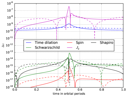
Figure 6: Redshift curves of terrestrial satellites. The dashed curves give the results for an orbit with the semi-major axis and eccentricity corresponding to the ones of the Galileo $5$ & $6$ satellites. The solid lines give the results for a typical satellite with high eccentricity while all the other Keplerian elements and the observer’s position were left the same.

V Conclusions

A spinning body causes spacetime to rotate around it, thus making nearby angular momentum vectors precess. This had already been considered theoretically in the early days of general relativity Lense and Thirring (1918). Only in recent years, however, has the effect entered the experimental realm Ciufolini and Pavlis (2004); Ciufolini et al. (2016); Everitt et al. (2011).

Frame-dragging is usually thought of as a steady precession. For highly eccentric orbits, however, this is far from the case. While having a minor impact along most of the orbit, frame-dragging kicks in around pericenter. This can be seen in Fig. 1 which shows the change of the longitude of ascending node due to spin for some example orbits of the Juno spacecraft. An analogous situation applies to the S stars in orbit around the Galactic-center black hole Angélil and Saha (2014). We suggest that these pericenter-kicks could provide a distinctive signature in timing signals obtained from spacecraft tracking.

The frame-dragging contribution to the redshift of spacecraft signals is

$$\Delta z_{\text{spin}}=-2\left(\frac{GM}{c^{2}r}\right)^{2}\vec{s}\cdot(\hat{r}\times\hat{b})$$ (22)

(given in geometrized units as in Eq. 10) where $\hat{b}$ is the line of sight to the spacecraft, and $\vec{s}$ is the dimensionless spin vector. Substituting the approximation expression (16) for the spin parameter, and assuming that the spacecraft has a low pericenter, so that $r_{\text{peri}}$ is of the same order as the planetary radius, gives

$$\Delta z_{\text{spin}}\sim\frac{GM}{c^{3}P}$$ (23)

where $P$ is the spin period. Jupiter has $GM/c^{3}\sim 5\,\rm nanosec$ and $P\sim 10\rm\,hr$, indicating $\Delta z_{\text{spin}}\sim 10^{-13}$. Furthermore, as Fig. 3 shows, the frame-dragging signal is concentrated over a duration of two hours around the pericenter.

In this paper we have modeled the effects of the curvature of the spacetime on both the orbit of a spacecraft and on the electromagnetic signals it sends to Earth. The aim is to quantify how the different relativistic effects influence the observable redshift signal. Geodesic equations are written in four dimensions in Hamiltonian form. Orbit equations for a spacecraft are a straightforward initial-value problem, while the equations for light signals traveling between the spacecraft and the observer form a boundary-value problem. Both sets of equations are solved numerically, using extended-precision floating point arithmetic, to compute redshift signals. Different metric terms are turned on and off to compare the signatures of each effect on the signal. We particularly focus on the spin terms, for which there are good predictions for the planets in our solar system. The eccentricity of the orbit can also increase the size of the terms by at least an order of magnitude.

Figures 2, 5 and 6 show example orbits of Juno, Cassini, and the eccentric Galileo spacecraft respectively. They also show the effect of the quadrupole $J_{2}$, which is orders of magnitude larger than the spin effect, but has a different time dependence. For the eccentric Galileo satellites, relativistic time dilation reaches $\sim 10^{-9}$ and is expected to be accurately measured; the leading order effects of a Schwarzschild spacetime are $\sim 10^{-13}$ and will be challenging; spin effects are two orders of magnitude smaller and hence unlikely to be measured. For both Juno and Cassini, spin effects reach $\sim 10^{-13}$ which is well above timing uncertainties.

Measurability centers on whether the frame-dragging signal can be disentangled from the much larger quadrupole and other “foreground” effects Finocchiaro et al. (2011); Tommei et al. (2015); Serra et al. (2016). The specific and known time-dependence of the frame-dragging signal offers some hope of doing so, but the question remains open.

References

- Iorio (2015) L. Iorio, Universe 1, 38 (2015).
- Debono and Smoot (2016) I. Debono and G. F. Smoot, Universe 2, 23 (2016), arXiv:1609.09781 [gr-qc] .
- Taylor (1994) J. H. Taylor, Rev. Mod. Phys. 66, 711 (1994).
- Kramer et al. (2006) M. Kramer, I. H. Stairs, R. N. Manchester, M. A. McLaughlin, A. G. Lyne, R. D. Ferdman, M. Burgay, D. R. Lorimer, A. Possenti, N. D’Amico, J. M. Sarkissian, G. B. Hobbs, J. E. Reynolds, P. C. C. Freire, and F. Camilo, Science 314, 97 (2006).
- Ciufolini and Pavlis (2004) I. Ciufolini and E. Pavlis, Nature 431, 958 (2004).
- Ciufolini et al. (2016) I. Ciufolini, A. Paolozzi, E. C. Pavlis, R. Koenig, J. Ries, V. Gurzadyan, R. Matzner, R. Penrose, G. Sindoni, C. Paris, H. Khachatryan, and S. Mirzoyan, European Physical Journal C 76, 120 (2016), arXiv:1603.09674 [gr-qc] .
- Iorio et al. (2011) L. Iorio, H. I. Lichtenegger, M. L. Ruggiero, and C. Corda, Astrophysics and Space Science 331, 351 (2011).
- Renzetti (2013) G. Renzetti, Open Physics 11, 531 (2013).
- Renzetti (2015) G. Renzetti, Acta Astronautica 113, 164 (2015).
- Iorio (2017) L. Iorio, The European Physical Journal C 77, 73 (2017).
- Everitt et al. (2011) C. F. Everitt, D. DeBra, B. Parkinson, J. Turneaure, J. Conklin, M. Heifetz, G. Keiser, A. Silbergleit, T. Holmes, J. Kolodziejczak, et al., Physical Review Letters 106, 221101 (2011).
- Ashby (2003) N. Ashby, Living Reviews in Relativity 6, 1 (2003).
- Cacciapuoti and Salomon (2011) L. Cacciapuoti and C. Salomon, in Journal of Physics: Conference Series, Vol. 327 (IOP Publishing, 2011) p. 012049.
- Altschul, B. et al. (2015) Altschul, B. et al., Advances in Space Research 55, 501 (2015).
- Bondarescu et al. (2012) R. Bondarescu, M. Bondarescu, G. Hetényi, L. Boschi, P. Jetzer, and J. Balakrishna, Geophysical Journal International 191, 78 (2012).
- Bondarescu et al. (2015) R. Bondarescu, A. Schärer, A. Lundgren, G. Hetényi, N. Houlié, P. Jetzer, and M. Bondarescu, Geophys. J. Int. 202, 1770 (2015).
- Lense and Thirring (1918) J. Lense and H. Thirring, Physikalische Zeitschrift 19 (1918).
- Helled et al. (2011) R. Helled, J. D. Anderson, G. Schubert, and D. J. Stevenson, Icarus 216, 440 (2011).
- Iorio (2013) L. Iorio, Classical and Quantum Gravity 30, 195011 (2013).
- Iorio (2010) L. Iorio, New Astronomy 15, 554 (2010).
- Iorio (2011) L. Iorio, Phys. Rev. D 84, 124001 (2011), arXiv:1107.2916 [gr-qc] .
- Iorio (2012) L. Iorio, General Relativity and Gravitation 44, 719 (2012), arXiv:1012.5622 [gr-qc] .
- Iorio, L. (2005) Iorio, L., A&A 431, 385 (2005).
- Park et al. (2017) R. S. Park, W. M. Folkner, A. S. Konopliv, J. G. Williams, D. E. Smith, and M. T. Zuber, The Astronomical Journal 153, 121 (2017).
- Angélil et al. (2014) R. Angélil, P. Saha, R. Bondarescu, P. Jetzer, A. Schärer, and A. Lundgren, Phys. Rev. D 89, 064067 (2014).
- Kannan and Saha (2009) R. Kannan and P. Saha, The Astrophysical Journal 690, 1553 (2009).
- Preto and Saha (2009) M. Preto and P. Saha, APJ 703, 1743 (2009), arXiv:0906.2226 [astro-ph.GA] .
- Angélil and Saha (2010) R. Angélil and P. Saha, The Astrophysical Journal 711, 157 (2010).
- Angélil et al. (2010) R. Angélil, P. Saha, and D. Merritt, The Astrophysical Journal 720, 1303 (2010).
- Angélil and Saha (2011) R. Angélil and P. Saha, APJL 734, L19 (2011), arXiv:1105.0918 .
- Angélil and Saha (2014) R. Angélil and P. Saha, MNRAS 444, 3780 (2014), arXiv:1408.0283 .
- Zhang and Iorio (2017) F. Zhang and L. Iorio, Astrophys. J. 834, 198 (2017), arXiv:1610.09781 .
- Duchayne, L. et al. (2009) Duchayne, L., Mercier, F., and Wolf, P., A&A 504, 653 (2009).
- Klioner and Kopeikin (1992) S. Klioner and S. Kopeikin, The Astronomical Journal 104, 897 (1992).
- Ashby and Bertotti (2010) N. Ashby and B. Bertotti, Classical and Quantum Gravity 27, 145013 (2010).
- Hees et al. (2014) A. Hees, S. Bertone, and C. Le Poncin-Lafitte, Phys. Rev. D 90, 084020 (2014).
- Crosta et al. (2015) M. Crosta, A. Vecchiato, F. de Felice, and M. G. Lattanzi, Classical and Quantum Gravity 32, 165008 (2015).
- D’Orazio and Saha (2010) D. J. D’Orazio and P. Saha, MNRAS 406, 2787 (2010), arXiv:1003.5659 [astro-ph.GA] .
- Kopeikin (1997) S. M. Kopeikin, J. Math. Phys. 38, 2587 (1997).
- Wex and Kopeikin (1999) N. Wex and S. M. Kopeikin, The Astrophysical Journal 514, 388 (1999).
- Mashhoon et al. (1984) B. Mashhoon, F. W. Hehl, and D. S. Theiss, General Relativity and Gravitation 16, 711 (1984).
- Helled (2011) R. Helled, The Astrophysical Journal Letters 735, L16 (2011).
- Nettelmann et al. (2015) N. Nettelmann, J. Fortney, K. Moore, and C. Mankovich, Monthly Notices of the Royal Astronomical Society 447, 3422 (2015).
- Zharkov and Trubitsyn (1980) V. N. Zharkov and V. P. Trubitsyn, Moscow, Izdatel’stvo Nauka, 1980. 448 p. In Russian. 1 (1980).
- Maistre et al. (2016) S. L. Maistre, W. Folkner, R. Jacobson, and D. Serra, Planetary and Space Science 126, 78 (2016).
- Guillot and Gautier (2007) T. Guillot and D. Gautier, “Treatise on geophysics, planets and moons, vol. 10,” (2007), arXiv:0912.2019 .
- Helled et al. (2010) R. Helled, J. D. Anderson, and G. Schubert, Icarus 210, 446 (2010).
- Helled et al. (2009) R. Helled, G. Schubert, and J. D. Anderson, Planetary and Space Science 57, 1467 (2009).
- Helled et al. (2015) R. Helled, E. Galanti, and Y. Kaspi, Nature 520, 202 (2015).
- Gurnett et al. (2007) D. Gurnett, A. Persoon, W. Kurth, J. Groene, T. Averkamp, M. Dougherty, and D. Southwood, Science 316, 442 (2007).
- Ingersoll and Pollard (1982) A. P. Ingersoll and D. Pollard, Icarus 52, 62 (1982).
- Sterenborg and Bloxham (2010) M. G. Sterenborg and J. Bloxham, Geophysical Research Letters 37 (2010).
- Anderson and Schubert (2007) J. D. Anderson and G. Schubert, Science 317, 1384 (2007).
- Read et al. (2009) P. Read, T. Dowling, and G. Schubert, Nature 460, 608 (2009).
- Matousek (2007) S. Matousek, Acta Astronautica 61, 932 (2007).
- Edgington and Spilker (2016) S. G. Edgington and L. J. Spilker, Nature Geoscience 9, 472 (2016).
- Delva et al. (2015) P. Delva, A. Hees, S. Bertone, E. Richard, and P. Wolf, Classical and Quantum Gravity 32, 232003 (2015).
- Finocchiaro et al. (2011) S. Finocchiaro, L. Iess, W. M. Folkner, and S. Asmar, AGU Fall Meeting Abstracts (2011).
- Tommei et al. (2015) G. Tommei, L. Dimare, D. Serra, and A. Milani, Monthly Notices of the Royal Astronomical Society 446, 3089 (2015).
- Serra et al. (2016) D. Serra, L. Dimare, G. Tommei, and A. Milani, Planetary and Space Science 134, 100 (2016).