LED-based Photometric Stereo: Modeling, Calibration and Numerical Solution

Abstract

We conduct a thorough study of photometric stereo under nearby point light source illumination, from modeling to numerical solution, through calibration. In the classical formulation of photometric stereo, the luminous fluxes are assumed to be directional, which is very difficult to achieve in practice. Rather, we use light-emitting diodes (LEDs) to illuminate the scene to be reconstructed. Such point light sources are very convenient to use, yet they yield a more complex photometric stereo model which is arduous to solve. We first derive in a physically sound manner this model, and show how to calibrate its parameters. Then, we discuss two state-of-the-art numerical solutions. The first one alternatingly estimates the albedo and the normals, and then integrates the normals into a depth map. It is shown empirically to be independent from the initialization, but convergence of this sequential approach is not established. The second one directly recovers the depth, by formulating photometric stereo as a system of nonlinear partial differential equations (PDEs), which are linearized using image ratios. Although the sequential approach is avoided, initialization matters a lot and convergence is not established either. Therefore, we introduce a provably convergent alternating reweighted least-squares scheme for solving the original system of nonlinear PDEs. Finally, we extend this study to the case of RGB images.

1 Introduction

3D-reconstruction is one of the most important goals of computer vision. Among the many techniques which can be used to accomplish this task, shape-from-shading Horn1989a and photometric stereo Woodham1980a are photometric techniques, as they use the relationship between the gray or color levels of the image, the shape of the scene, supposedly opaque, its reflectance and the luminous flux that illuminates it.

Let us first introduce some notations that will be used throughout this paper. We describe a point $\mathbf{x}$ on the scene surface by its coordinates $[x,y,z]^{\top}$ in a frame originating from the optical center $C$ of the camera, such that the plane $Cxy$ is parallel to the image plane and the $Cz$ axis coincides with the optical axis and faces the scene (cf. Fig. 1). The coordinates $[u,v]^{\top}$ of a point $\mathbf{p}$ in the image (pixel) are relative to a frame $Ouv$ whose origin is the principal point $O$, and whose axes $Ou$ and $Ov$ are parallel to $Cx$ and $Cy$, respectively. If $f$ refers to the focal length, the conjugation relationship between $\mathbf{x}$ and $\mathbf{p}$ is written, in perspective projection:

$$\begin{cases}x=\dfrac{z}{f}\,u,\\[10.00002pt] y=\dfrac{z}{f}\,v.\end{cases}$$ (1.1)

Figure 1: Schematic representation of the geometric setup. A point $\mathbf{x}=[x,y,z]^{\top}\in\mathbb{R}^{3}$ on the scene surface and a pixel $\mathbf{p}=[u,v]^{\top}\in\mathbb{R}^{2}$ in the image plane are conjugated according to Eq. (1.1). Eq. (2.1) states that, when the scene is illuminated by a LED located in $\mathbf{x}_{s}\in\mathbb{R}^{3}$, the gray level $I(\mathbf{p})$ of the pixel $\mathbf{p}$ conjugated to $\mathbf{x}$ is a function of the angle between the lighting vector $\mathbf{s}(\mathbf{x})$ and the normal $\mathbf{n}(\mathbf{x})$ to the surface in $\mathbf{x}$ (illuminance), of the angle $\theta$ between the principal direction $\mathbf{n}_{s}$ of the LED and $\mathbf{s}(\mathbf{x})$ (anisotropy), of the distance $\|\mathbf{x}-\mathbf{x}_{s}\|$ between the surface point and the light source location (inverse-of-square falloff), and of the albedo in $\mathbf{x}$ (Lambertian reflectance).

The 3D-reconstruction problem consists in estimating, in each pixel $\mathbf{p}$ of a part $\Omega$ of the image domain, its conjugate point $\mathbf{x}$ in 3D-space. Eq. (1.1) shows that it suffices to find the depth $z$ to determine $\mathbf{x}=\left[x,y,z\right]^{\top}$ from $\mathbf{p}=\left[u,v\right]^{\top}$. The only unknown of the problem is thus the depth map $z$, which is defined as follows:

$$\begin{array}[]{rccl}z\,:&\Omega\subset\mathbb{R}^{2}&\to&\mathbb{R}^{+}\\ {}\hfil&\mathbf{p}=[u,v]^{\top}&\mapsto&z(\mathbf{p}).\end{array}$$ (1.2)

We are interested in this article in 3D-reconstruction of Lambertian surfaces by photometric stereo. The reflectance in a point of such a surface is completely characterized by a coefficient $\rho$, called albedo, which is 0 if the point is black and 1 if it is white. Photometric stereo is nothing else than an extension of shape-from-shading: instead of a single image, the former uses $m\geqslant$ 3 shots $I^{i},\,i\in\{1,\dots,m\}$, taken from the same angle, but under varying lighting. Considering multiple images allows to circumvent the difficulties of shape-from-shading: photometric stereo techniques are able to unambiguously estimate the 3D-shape as well as the albedo i.e., without resorting to any prior.

A parallel and uniform illumination can be characterized by a vector $\mathbf{s}\in\mathbb{R}^{3}$ oriented towards the light source, whose norm is equal to the luminous flux density. We call $\mathbf{s}$ the lighting vector. For a Lambertian surface, the classical modeling of photometric stereo is written, in each pixel $\mathbf{p}\in\Omega$, as the following system:

$$I^{i}(\mathbf{p})=\rho(\mathbf{x})\,\,\mathbf{s}^{i}\cdot\mathbf{n}(\mathbf{x}),\qquad i\in\{1,\dots,m\},$$ (1.3)

where $I^{i}(\mathbf{p})$ denotes the gray level of $\mathbf{p}$ under a parallel and uniform illumination characterized by the lighting vector $\mathbf{s}^{i}$, $\rho(\mathbf{x})$ denotes the albedo in the point $\mathbf{x}$ conjugate to $\mathbf{p}$, and ${\mathbf{n}}(\mathbf{x})$ denotes the unit-length outgoing normal to the surface in this point. Since there is a one-to-one correspondence between the points $\mathbf{x}$ and the pixels $\mathbf{p}$, we write for convenience $\rho(\mathbf{p})$ and $\mathbf{n}(\mathbf{p})$, in lieu of $\rho(\mathbf{x})$ and $\mathbf{n}(\mathbf{x})$. Introducing the notation $\mathbf{m}(\mathbf{p})=\rho(\mathbf{p})\,\mathbf{n}(\mathbf{p})$, System (1.3) can be rewritten in matrix form:

$$\mathbf{I}(\mathbf{p})=\mathbf{S}\,\mathbf{m}(\mathbf{p}),$$ (1.4)

where vector $\mathbf{I}(\mathbf{p})\in\mathbb{R}^{m}$ and matrix $\mathbf{S}\in\mathbb{R}^{m\times 3}$ are defined as follows:

$$\mathbf{I}(\mathbf{p})=\begin{bmatrix}I^{1}(\mathbf{p})\\ \vdots\\ I^{m}(\mathbf{p})\end{bmatrix}\qquad\text{and}\qquad\mathbf{S}=\begin{bmatrix}\mathbf{s}^{1\top}\\ \vdots\\ \mathbf{s}^{m\top}\end{bmatrix}.$$ (1.5)

As soon as $m\geqslant 3$ non-coplanar lighting vectors are used, matrix $\mathbf{S}$ has rank 3. The (unique) least-squares solution of System (1.4) is then given by

$$\mathbf{m}(\mathbf{p})=\mathbf{S}^{\dagger}\,\mathbf{I}(\mathbf{p}),$$ (1.6)

where $\mathbf{S}^{\dagger}$ is the pseudo-inverse of $\mathbf{S}$. From this solution, we easily deduce the albedo and the normal:

$$\rho(\mathbf{p})=\|\mathbf{m}(\mathbf{p})\|\qquad\text{and}\qquad\mathbf{n}(\mathbf{p})=\frac{\mathbf{m}(\mathbf{p})}{\|\mathbf{m}(\mathbf{p})\|}.$$ (1.7)

The normal field estimated in such a way must eventually be integrated so as to obtain the depth map, knowing that the boundary conditions, the shape of domain $\Omega$ as well as depth discontinuities significantly complicate this task Durou2016 .

To ensure lighting directionality, as is required by Model (1.3), it is necessary to achieve a complex optical setup Moreno2006 . It is much easier to use light-emitting diodes (LEDs) as light sources, but with this type of light sources, we should expect significant changes in the modeling, and therefore in the numerical solution. The aim of our work is to conduct a comprehensive and detailed study of photometric stereo under point light source illumination such as LEDs.

Related works.

Modeling the luminous flux emitted by a LED is a well-studied problem, see for instance Moreno2008 . One model which is frequently considered in computer vision is that of nearby point light source. This model involves an inverse-of-square law for describing the attenuation of lighting intensity with respect to distance, which has long been identified as a key feature for solving shape-from-shading Iwahori1990 and photometric stereo Clark1992 . Attenuation with respect to the deviation from the principal direction of the source (anisotropy) has also been considered Bennahmias2007 .

If the surface to reconstruct lies in the vicinity of a plane, it is possible to capture a map of this attenuation using a white planar reference object. Conventional photometric stereo Woodham1980a can then be applied to the images compensated by the attenuation maps Angelopoulou2014a ; McGunnigle2003 ; Sun2013 . Otherwise, it is necessary to include the attenuation coefficients in the photometric stereo model, which yields a nonlinear inverse problem to be solved.

This is easier to achieve if the parameters of the illumination model have been calibrated beforehand. Lots of methods exist for estimating a source location Ackermann2013 ; Aoto2012 ; Ciortan2016 ; Giachetti2015 ; Hara2005 ; Powell2001 ; Shen2011 ; Takai2009 . Such methods triangulate this location during a calibration procedure, by resorting to specular spheres. This can also be achieved online, by introducing spheres in the scene to reconstruct Liao2016 . Calibrating anisotropy is a more challenging problem, which was tackled recently in Nie2016 ; Xie2015b by using images of a planar surface. Some photometric stereo methods also circumvent calibration by (partly or completely) automatically inferring lighting during the 3D-reconstruction process Koppal2007 ; Liao2016 ; Logothetis2017 ; Migita2008 ; Papadhimitri2014b ; SSVM2017 .

Still, even in the calibrated case, designing numerical schemes for solving photometric stereo under nearby point light sources remains difficult. When only two images are considered, the photometric stereo model can be simplified using image ratios. This yields a quasilinear PDE Mecca2015 ; Mecca2014b which can be solved by provably convergent front propagation techniques, provided that a boundary condition is known. To improve robustness, this strategy has been adapted to the multi-images case in Logothetis2017 ; Logothetis_2016 ; Mecca2016 ; CVPR2016 , using variational methods. However, convergence guarantees are lost. Instead of considering such a differential approach, another class of methods Ahmad2014 ; Bony2013 ; Collins2012 ; Huang2015 ; Kolagani1992 ; Nie2016b ; Papadhimitri2014b ; Yeh2016 rather modify the classical photometric stereo framework Woodham1980a , by alternatingly estimating the normals and the albedo, integrating the normals into a depth map, and updating the lighting based on the current depth. Yet, no convergence guarantee does exist. A method based on mesh deformation has also been proposed in Xie2015 , but convergence is not established either.

Contributions.

In contrast to existing works which focus either on modeling, calibrating or solving photometric stereo with near point light sources such as LEDs, the objective of this article is to propose a comprehensive study of all these aspects of the problem. Building upon our previous conference papers CVPR2016 ; SSVM2017 ; CVPR2017 , we introduce the following innovations:

• We present in Section 2 an accurate model for photometric stereo under point light source illumination. As in recent works Logothetis2017 ; Logothetis_2016 ; Mecca2015 ; Mecca2014b ; Mecca2016 ; Nie2016b ; Nie2016 ; Xie2015b , this model takes into account the nonlinearities due to distance and to the anisotropy of the LEDs. Yet, it also clarifies the notions of albedo and of source intensity, which are shown to be relative to a reference albedo and to several parameters of the camera, respectively. This section also introduces a practical calibration procedure for the location, the orientation and the relative intensity of the LEDs.
  

• Section 3 reviews and improves two state-of-the-art numerical solutions in several manners. We first modify the alternating method Ahmad2014 ; Bony2013 ; Collins2012 ; Huang2015 ; Kolagani1992 ; Nie2016b ; Papadhimitri2014b ; Yeh2016 by introducing an estimation of the shape scale, in order to recover the absolute depth without any prior. We then study the PDE-based approach which employs image ratios for eliminating the nonlinearities Logothetis2017 ; Logothetis_2016 ; Mecca2016 ; CVPR2016 , and empirically show that local minima can be avoided by employing an augmented Lagrangian strategy. Nevertheless, neither of these state-of-the-art methods is provably convergent.
  

• Therefore, we introduce in Section 4 a new, provably convergent method, inspired by the one recently proposed in SSVM2017 . It is based on a tailored alternating reweighted least-squares scheme for approximately solving the non-linearized system of PDEs. Following CVPR2017 , we further show that this method is easily extended in order to address shadows and specularities.
  

• In Section 5, we build upon the analysis conducted in CVPR2016 in order to tackle the case of RGB-valued images, before concluding and suggesting several future research directions in Section 6.

2 Photometric Stereo under Point Light Source Illumination

Conventional photometric stereo Woodham1980a assumes that the primary luminous fluxes are parallel and uniform, which is difficult to guarantee. It is much easier to illuminate a scene with LEDs.

Keeping this in mind, we have developed a photometric stereo-based setup for 3D-reconstruction of faces, which includes $m=8$ LEDs located at about $30~{}cm$ from the scene surface (see Fig. 2-a). The face is photographed by a Canon EOS 7D camera with focal length $f=35~{}mm$. Triggering the shutter in burst mode, while synchronically lighting the LEDs, provides us with $m=8$ images such as those of Figs. 2-b, 2-c and 2-d. In this section, we aim at modeling the formation of such images, by establishing the following result: 

If the $m$ LEDs are modeled as anisotropic (imperfect Lambertian) point light sources, if the surface is Lambertian and if all the automatic settings of the camera are deactivated, then the formation of the $m$ images can be modeled as follows, for $i\in\{1,\dots,m\}$:

$$I^{i}(\mathbf{p})=\Psi^{i}\,\overline{\rho}(\mathbf{p})\left[\frac{\mathbf{n}^{i}_{s}\!\cdot\!\left(\mathbf{x}\!-\!\mathbf{x}^{i}_{s}\right)}{\|\mathbf{x}\!-\!\mathbf{x}^{i}_{s}\|}\right]^{\mu^{i}}\!\!\frac{\left\{(\mathbf{x}^{i}_{s}\!-\!\mathbf{x})\cdot\mathbf{n}(\mathbf{p})\right\}_{+}}{\|\mathbf{x}^{i}_{s}\!-\!\mathbf{x}\|^{3}},$$ (2.1)

where:

• $I^{i}(\mathbf{p})$ is the “corrected gray level” at pixel $\mathbf{p}$ conjugate to a point $\mathbf{x}$ located on the surface (cf. Eq. (2.12));

• $\Psi^{i}$ is the intensity of the $i$-th source multiplied by an unknown factor, which is common to all the sources and depends on several camera parameters and on the albedo $\rho_{0}$ of a Lambertian planar calibration pattern (cf. Eq. (2.14));

• $\overline{\rho}(\mathbf{p})$ is the albedo of the surface point $\mathbf{x}$ conjugate to pixel $\mathbf{p}$, relatively to $\rho_{0}$ (cf. Eq. (2.22));

• $\mathbf{n}^{i}_{s}\in\mathbb{S}^{2}\subset\mathbb{R}^{3}$ is the (unit-length) principal direction of the $i$-th source, $\mathbf{x}^{i}_{s}\in\mathbb{R}^{3}$ its location (cf. Fig. 2), and $\mu^{i}\geq 0$ its anisotropy parameter (cf. Fig. 3 and Eq. (2.5));

• $\{\cdot\}_{+}$ is the positive part operator, which accounts for self-shadows:

  $$\{x\}_{+}=\max\{x,0\}.$$ (2.2)

In Eq. (2.1), the anisotropy parameters $\mu^{i}$ are (indirectly) provided by the manufacturer (cf. Eq. (2.6)), and the other LEDs parameters $\Psi^{i}$, $\mathbf{n}^{i}_{s}$ and $\mathbf{x}^{i}_{s}$ can be calibrated thanks to the procedure described in Section 2.2. The only unknowns in System (2.1) are thus the depth $z$ of the 3D-point $\mathbf{x}$ conjugate to $\mathbf{p}$, its (relative) albedo $\overline{\rho}(\mathbf{p})$ and its normal $\mathbf{n}(\mathbf{p})$. The estimation of these unknowns will be discussed in Sections 3 and 4. Before that, let us show step-by-step how to derive Eq. (2.1).

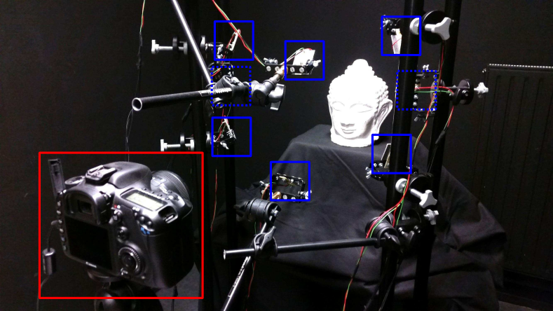
(a)

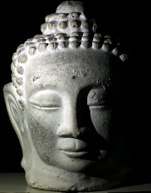
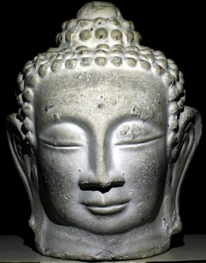
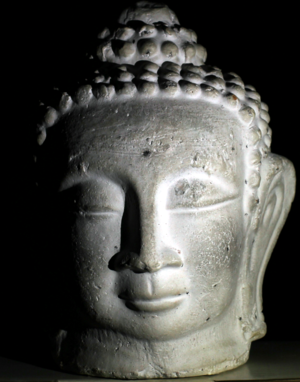
(b)	(c)	(d)

Figure 2: (a) Our photometric stereo-based experimental setup for 3D-reconstruction of faces using a Canon EOS 7D camera (highlighted in red) and $m=8$ LEDs (highlighted in blue). The walls are painted in black in order to avoid the reflections between the scene and the environment. (b-c-d) Three out of the $m=8$ images obtained by this setup.

2.1 Modeling the Luminous Flux Emitted by a LED

For the LEDs we use, the characteristic illuminating volume is of the order of one cubic millimeter. Therefore, in comparison with the scale of a face, each LED can be seen as a point light source located at $\mathbf{x}_{s}\in\mathbb{R}^{3}$. At any point $\mathbf{x}\in\mathbb{R}^{3}$, the lighting vector $\mathbf{s}(\mathbf{x})$ is necessarily radial i.e., collinear with the unit-length vector $\textbf{u}_{r}=\frac{\mathbf{x}-\mathbf{x}_{s}}{\|\mathbf{x}-\mathbf{x}_{s}\|}$. Using spherical coordinates $(r,\theta,\phi)$ of $\mathbf{x}$ in a frame having $\mathbf{x}_{s}$ as origin, it is written

$$\mathbf{s}(\mathbf{x})=-\frac{\Phi(\theta,\phi)}{r^{2}}\,\textbf{u}_{r},$$ (2.3)

where $\Phi(\theta,\phi)\geqslant 0$ denotes the intensity of the source, and the $1/r^{2}$ attenuation is a consequence of the conservation of luminous energy in a non-absorbing medium. Vector $\mathbf{s}(\mathbf{x})$ is purposely oriented in the opposite direction from that of the light, in order to simplify the writing of the Lambertian model.

Model (2.3) is very general. We could project the intensity $\Phi(\theta,\phi)$ on the spherical harmonics basis, which allowed Basri et al. to model the luminous flux in the case of uncalibrated photometric stereo Basri2003 . We could also sample $\Phi(\theta,\phi)$ in the vicinity of a plane, using a plane with known reflectance Angelopoulou2014a ; McGunnigle2003 ; Sun2013 .

Using the specific characteristics of LEDs may lead to a more accurate model. Indeed, most of the LEDs emit a luminuous flux which is invariant by rotation around a principal direction indicated by a unit-length vector $\mathbf{n}_{s}$ Moreno2008 . If $\theta$ is defined relatively to $\mathbf{n}_{s}$, this means that $\Phi(\theta,\phi)$ is independent from $\phi$. The lighting vector in $\mathbf{x}$ induced by a LED located in $\mathbf{x}_{s}$ is thus written

$$\mathbf{s}(\mathbf{x})=\frac{\Phi(\theta)}{\|\mathbf{x}_{s}-\mathbf{x}\|^{2}}\,\frac{\mathbf{x}_{s}-\mathbf{x}}{\|\mathbf{x}_{s}-\mathbf{x}\|}.$$ (2.4)

The dependency on $\theta$ of the intensity $\Phi$ characterizes the anisotropy of the LED. The function $\Phi(\theta)$ is generally decreasing over $[0,\pi/2]$ (cf. Fig. 3).

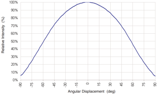
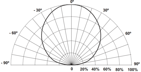
(a)	(b)

Figure 3: Intensity patterns of the LEDs used (source: http://www.lumileds.com/uploads/28/DS64-pdf). (a) Anisotropy function $\Phi(\theta)/\Phi_{0}$ as a function of $\theta$. (b) Polar representation. These diagrams show us that $\theta_{1/2}=\pi/3$, which corresponds to $\mu=1$ according to Eq. (2.6) (Lambertian source).

An anisotropy model satisfying this constraint is that of “imperfect Lambertian source”:

$$\Phi(\theta)=\Phi_{0}\,\cos^{\mu}\theta,$$ (2.5)

which contains two parameters $\Phi_{0}=\Phi(0)$ and $\mu\geqslant 0$, and models both isotropic sources ($\mu=0$) and Lambertian sources ($\mu=1$). Model (2.5) is empirical, and more elaborate models are sometimes considered Moreno2008 , yet it has already been used in photometric stereo Logothetis2017 ; Logothetis_2016 ; Mecca2016 ; Mecca2015 ; Nie2016b ; Nie2016 ; SSVM2017 ; Xie2015b , including the case where all the LEDs are arranged on a plane parallel to the image plane, in such a way that $\mathbf{n}_{s}=[0,0,1]^{\top}$ Mecca2014b . Model (2.5) has proven itself and, moreover, LEDs manufacturers provide the angle $\theta_{1/2}$ such that $\Phi(\theta_{1/2})=\Phi_{0}/2$, from which we deduce, using (2.5), the value of $\mu$:

$$\mu=-\frac{\log(2)}{\log(\cos\theta_{1/2})}.$$ (2.6)

As shown in Fig. 3, the angle $\theta_{1/2}$ is $\pi/3$ for the LEDs we use. From Eq. (2.6), we deduce that $\mu=1$, which means that these LEDs are Lambertian. Plugging the expression (2.5) of $\Phi(\theta)$ into (2.4), we obtain

$$\mathbf{s}(\mathbf{x})=\Phi_{0}\,\cos^{\mu}\theta\,\frac{\mathbf{x}_{s}-\mathbf{x}}{\|\mathbf{x}_{s}-\mathbf{x}\|^{3}},$$ (2.7)

where we explicitly keep $\mu$ to address the most general case. Model (2.7) thus includes seven parameters: three for the coordinates of $\mathbf{x}_{s}$, two for the unit vector $\mathbf{n}_{s}$, plus $\Phi_{0}$ and $\mu$. Note that $\mathbf{n}_{s}$ appears in this model through the angle $\theta$.

In its uncalibrated version, photometric stereo allows the 3D-reconstruction of a scene surface without knowing the lighting. Uncalibrated photometric stereo has been widely studied, including the case of nearby point light sources Huang2015 ; Koppal2007 ; Migita2008 ; Papadhimitri2014b ; Yeh2016 , but if this is possible, we should rather calibrate the lighting.

2.2 Calibrating the Luminous Flux Emitted by a LED

Most calibration methods of a point light source Ackermann2013 ; Aoto2012 ; Ciortan2016 ; Giachetti2015 ; Hara2005 ; Powell2001 ; Shen2011 ; Takai2009 do not take into account the attenuation of the luminous flux density as a function of the distance to the source, nor the possible anisotropy of the source, which may lead to relatively imprecise results. To our knowledge, there are few calibration procedures taking into account these phenomena. In Xie2015b , Xie et al. use a single pattern, which is partially specular and partially Lambertian, to calibrate a LED. We intend to improve this procedure using two patterns, one specular and the other Lambertian. The specular one will be used to determine the location of the LEDs by triangulation, and the Lambertian one to determine some other parameters by minimizing the reprojection error, as recently proposed by Pintus et al. in Pintus2016 .

Specular Spherical Calibration Pattern.

The location $\mathbf{x}_{s}$ of a LED can be determined by triangulation. In Powell2001 , Powell et al. advocate the use of a spherical mirror. To estimate the locations of the $m=8$ LEDs for our setup, we use a billiard ball. Under perspective projection, the edge of the silhouette of a sphere is an ellipse, which we detect using a dedicated algorithm Patraucean2012 . It is then easy to determine the 3D-coordinates of any point on the surface, as well as its normal, since the radius of the billiard ball is known. For each pose of the billiard ball, detecting the reflection of the LED allows us to determine, by reflecting the line of sight on the spherical mirror, a line in 3D-space passing through $\mathbf{x}_{s}$. In theory, two poses of the billiard ball are enough to estimate $\mathbf{x}_{s}$, even if two lines in 3D-space do not necessarily intersect, but the use of ten poses improves the robustness of the estimation.

Lambertian Model.

To estimate the principal direction $\mathbf{n}_{s}$ and the intensity $\Phi_{0}$ in Model (2.7), we use a Lambertian calibration pattern. A surface is Lambertian if the apparent clarity of any point $\mathbf{x}$ located on it is independent from the viewing angle. The luminance $L(\mathbf{x})$, which is equal to the luminous flux emitted per unit of solid angle and per unit of apparent surface, is independent from the direction of emission. However, the luminance is not characteristic of the surface, as it depends on the illuminance $E(\mathbf{x})$ (denoted $E$ from French “ clairement”), that is to say on the luminous flux per unit area received by the surface in $\mathbf{x}$. The relationship between luminance and illuminance is written, for a Lambertian surface:

$$L(\mathbf{x})=\frac{\rho(\mathbf{x})}{\pi}\,E(\mathbf{x}),$$ (2.8)

where the albedo $\rho(\mathbf{x})\in[0,1]$ is defined as the proportion of luminous energy which is reemitted i.e., $\rho(\mathbf{x})=1$ if $\mathbf{x}$ is white, and $\rho(\mathbf{x})=0$ if it is black.

The parameter $\rho(\mathbf{x})$ is enough to characterize the reflectance of a Lambertian surface. In addition, the illuminance at a point $\mathbf{x}$ of a (not necessarily Lambertian) surface with normal $\mathbf{n}(\mathbf{x})$, lit by the lighting vector $\mathbf{s}(\mathbf{x})$, is written

$$E(\mathbf{x})=\left\{\mathbf{s}(\mathbf{x})\cdot\mathbf{n}(\mathbf{x})\right\}_{+}.$$ (2.9)

Focusing the camera on a point $\mathbf{x}$ of the scene surface, the illuminance $\epsilon(\mathbf{p})$ of the image plane, at pixel $\mathbf{p}$ conjugate to $\mathbf{x}$, is related to the luminance $L(\mathbf{x})$ by the following “almost linear” relationship Horn1986 :

$$\epsilon(\mathbf{p})=\beta\,\cos^{4}\alpha(\mathbf{p})\,L(\mathbf{x}),$$ (2.10)

where $\beta$ is a proportionality coefficient characterizing the clarity of the image, which depends on several factors such as the lens aperture, the magnification, etc. Regarding the factor $\cos^{4}\alpha(\mathbf{p})$, where $\alpha(\mathbf{p})$ is the angle between the line of sight and the optical axis, it is responsible for darkening at the periphery of the image. This effect should not be confused with vignetting, since it occurs even with ideal lenses Gardner1947 .

With current photosensitive receptors, the gray level $J(\mathbf{p})$ at pixel $\mathbf{p}$ is almost proportional to its illuminance $\epsilon(\mathbf{p})$, except of course in case of saturation. Denoting $\gamma$ this coefficient of quasi-proportionality, and combining equalities (2.8), (2.9) and (2.10), we get the following expression of the gray level in a pixel $\mathbf{p}$ conjugate to a point $\mathbf{x}$ located on a Lambertian surface:

$$J(\mathbf{p})=\gamma\,\beta\,\cos^{4}\alpha(\mathbf{p})\,\frac{\rho(\mathbf{x})}{\pi}\,\left\{\mathbf{s}(\mathbf{x})\cdot\mathbf{n}(\mathbf{x})\right\}_{+}.$$ (2.11)

We have already mentioned that there is a one-to-one correspondence between a point $\mathbf{x}$ and its conjugate pixel $\mathbf{p}$, which allows us to denote $\rho(\mathbf{p})$ and $\mathbf{n}(\mathbf{p})$ instead of $\rho(\mathbf{x})$ and $\mathbf{n}(\mathbf{x})$. As the factor $\cos^{4}\alpha(\mathbf{p})$ is easy to calculate in each pixel $\mathbf{p}$ of the photosensitive receptor, since $\cos\alpha(\mathbf{p})=\frac{f}{\sqrt{\|\mathbf{p}\|^{2}+f^{2}}}$, we can very easily compensate for this source of darkening and will manipulate from now on the “corrected gray level”:

$$I(\mathbf{p})=\frac{J(\mathbf{p})}{\cos^{4}\alpha(\mathbf{p})}=\gamma\,\beta\,\frac{\rho(\mathbf{p})}{\pi}\,\left\{\mathbf{s}(\mathbf{x})\cdot\mathbf{n}(\mathbf{p})\right\}_{+}.$$ (2.12)

Lambertian Planar Calibration Pattern.

To estimate the parameters $\mathbf{n}_{s}$ and $\Phi_{0}$ in Model (2.7) i.e., to achieve photometric calibration, we use a second calibration pattern consisting of a checkerboard printed on a white paper sheet, which is itself stuck on a plane (cf. Fig. 4), with the hope that the unavoidable outliers to the Lambertian model will not influence the accuracy of the estimates too much.

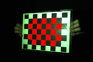
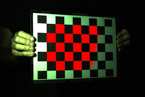
(a)	(b)

Figure 4: Two out of the $q$ poses of the Lambertian planar calibration pattern used for the photometric calibration of the LEDs. The parts of the white cells which are used for estimating the LEDs principal directions and intensities are highlighted in red.

The use of a convex calibration pattern (planar, in this case) has a significant advantage: the lighting vector $\mathbf{s}(\mathbf{x})$ at any point $\mathbf{x}$ of the surface is purely primary i.e., it is only due to the light source, without “bouncing” on other parts of the surface of the target, provided that the walls and surrounding objects are covered in black (see Fig. 2-a). Thanks to this observation, we can replace the lighting vector $\mathbf{s}(\mathbf{x})$ in Eq. (2.12) by the expression (2.7) which models the luminous flux emitted by a LED. From (2.7) and (2.12), we deduce the gray level $I(\mathbf{p})$ of the image of a point $\mathbf{x}$ located on this calibration pattern, illuminated by a LED:

$$I(\mathbf{p})=\gamma\,\beta\,\frac{\rho(\mathbf{p})}{\pi}\,\Phi_{0}\cos^{\mu}\!\theta\frac{\left\{(\mathbf{x}_{s}-\mathbf{x})\!\cdot\!\mathbf{n}(\mathbf{p})\right\}_{+}}{\|\mathbf{x}_{s}-\mathbf{x}\|^{3}}.$$ (2.13)

If $q\geqslant 3$ poses of the checkerboard are used, numerous algorithms exist for unambiguously estimating the coordinates of the points $\mathbf{x}^{j}$ of the pattern, for the different poses $j\in\{1,\dots,q\}$. These algorithms also allow the estimation of the $q$ normals $\mathbf{n}^{j}$ (we omit the dependency in $\mathbf{p}$ of $\mathbf{n}^{j}$, since the pattern is planar), and the intrinsic parameters of the camera. As for the albedo, if the use of white paper does not guarantee that $\rho(\mathbf{p})\equiv 1$, it still seems reasonable to assume $\rho(\mathbf{p})\equiv\rho_{0}$ i.e., to assume a uniform albedo in the white cells. We can then group all the multiplicative coefficients of the right hand side of Eq. (2.13) into one coefficient

$$\Psi=\gamma\,\beta\,\frac{\rho_{0}}{\pi}\,\Phi_{0}.$$ (2.14)

With this definition, and knowing that $\theta$ is the angle between vectors $\mathbf{n}_{s}$ and $\mathbf{x}-\mathbf{x}_{s}$, Eq. (2.13) can be rewritten, in a pixel $\mathbf{p}$ of the set $\Omega^{j}$ containing the white pixels of the checkerboard in the $j\textsuperscript{th}$ pose (these pixels are highlighted in red in the images of Fig. 4):

$$I^{j}(\mathbf{p})=\Psi\left[\displaystyle\frac{\mathbf{n}_{s}\cdot\left(\mathbf{x}^{j}-\mathbf{x}_{s}\right)}{\|\mathbf{x}^{j}-\mathbf{x}_{s}\|}\right]^{\mu}\displaystyle\frac{\left\{(\mathbf{x}_{s}-\mathbf{x}^{j})\cdot\mathbf{n}^{j}\right\}_{+}}{\|\mathbf{x}_{s}-\mathbf{x}^{j}\|^{3}}.$$ (2.15)

To be sure that in Eq. (2.15), $\Psi$ is independent from the pose $j$, we must deactivate all automatic settings of the camera, in order to make $\beta$ and $\gamma$ constant.

Since $\mathbf{x}_{s}$ is already estimated, and the value of $\mu$ is known, the only unknowns in Eq. (2.15) are $\mathbf{n}_{s}$ and $\Psi$. Two cases may occur:

• If the LED to calibrate is isotropic i.e., if $\mu=0$, then it is useless to estimate $\mathbf{n}_{s}$, and $\Psi$ can be estimated in a least-squares sense, by solving

  $$\underset{\Psi}{\operatorname{\min}~{}}\sum_{j=1}^{q}\sum_{\mathbf{p}\in\Omega^{j}}\left[I^{j}(\mathbf{p})-\Psi\,\frac{\left\{(\mathbf{x}_{s}-\mathbf{x}^{j})\cdot\mathbf{n}^{j}\right\}_{+}}{\|\mathbf{x}_{s}-\mathbf{x}^{j}\|^{3}}\right]^{2},$$ (2.16)

  whose solution is given by

  $$\Psi=\displaystyle\frac{\displaystyle\sum_{j=1}^{q}\sum_{\mathbf{p}\in\Omega^{j}}I^{j}(\mathbf{p})\,\displaystyle\frac{\left\{(\mathbf{x}_{s}-\mathbf{x}^{j})\cdot\mathbf{n}^{j}\right\}_{+}}{\|\mathbf{x}_{s}-\mathbf{x}^{j}\|^{3}}}{\displaystyle\sum_{j=1}^{q}\sum_{\mathbf{p}\in\Omega^{j}}\left[\displaystyle\frac{\left\{(\mathbf{x}_{s}-\mathbf{x}^{j})\cdot\mathbf{n}^{j}\right\}_{+}}{\|\mathbf{x}_{s}-\mathbf{x}^{j}\|^{3}}\right]^{2}}.$$ (2.17)

• Otherwise (if $\mu>0$), Eq. (2.15) can be rewritten

  $$\underbrace{\Psi^{\frac{1}{\mu}}\,\mathbf{n}_{s}}_{\mathbf{m}_{s}}\cdot\,(\mathbf{x}^{j}\!-\!\mathbf{x}_{s})\!=\!\left[\!\displaystyle I^{j}(\mathbf{p})\,\frac{\|\mathbf{x}_{s}-\mathbf{x}^{j}\|^{3+\mu}}{\left\{(\mathbf{x}_{s}\!-\!\mathbf{x}^{j})\!\cdot\!\mathbf{n}^{j}\!\right\}_{+}}\right]^{\frac{1}{\mu}}\!\!.$$ (2.18)

  The least-squares estimation of vector $\mathbf{m}_{s}$ defined in (2.18) is thus written

  $$\underset{\mathbf{m}_{s}}{\operatorname{\min}~{}}\sum_{j=1}^{q}\sum_{\mathbf{p}\in\Omega^{j}}\!\left[\!\mathbf{m}_{s}\cdot(\mathbf{x}^{j}\!-\!\mathbf{x}_{s})\!-\!\left[\!\displaystyle I^{j}(\mathbf{p})\,\frac{\|\mathbf{x}_{s}\!-\!\mathbf{x}^{j}\|^{3+\mu}}{\left\{(\mathbf{x}_{s}\!-\!\mathbf{x}^{j})\cdot\mathbf{n}^{j}\right\}_{+}}\right]^{\frac{1}{\mu}}\right]^{2}.$$ (2.19)

  This linear least-squares problem can be solved using the pseudo-inverse. From this estimate, we easily deduce those of parameters $\mathbf{n}_{s}$ and $\Psi$:

  $$\mathbf{n}_{s}=\frac{\mathbf{m}_{s}}{\|\mathbf{m}_{s}\|}\qquad\text{and}\qquad\Psi=\|\mathbf{m}_{s}\|^{\mu}.$$ (2.20)

In both cases, it is impossible to deduce from the estimate of $\Psi$ that of $\Phi_{0}$, because in the definition (2.14) of $\Psi$, the product $\gamma\,\beta\,\frac{\rho_{0}}{\pi}$ is unknown. However, since this product is the same for all LEDs (deactivating all automatic settings of the camera makes $\beta$ and $\gamma$ constant), all the intensities $\Phi_{0}^{i}$, $i\in\{1,\dots,m\}$, are estimated up to a common factor.

Fig. 5 shows a schematic representation of the experimental setup of Fig. 2-a, where the LEDs parameters were estimated using our calibration procedure.

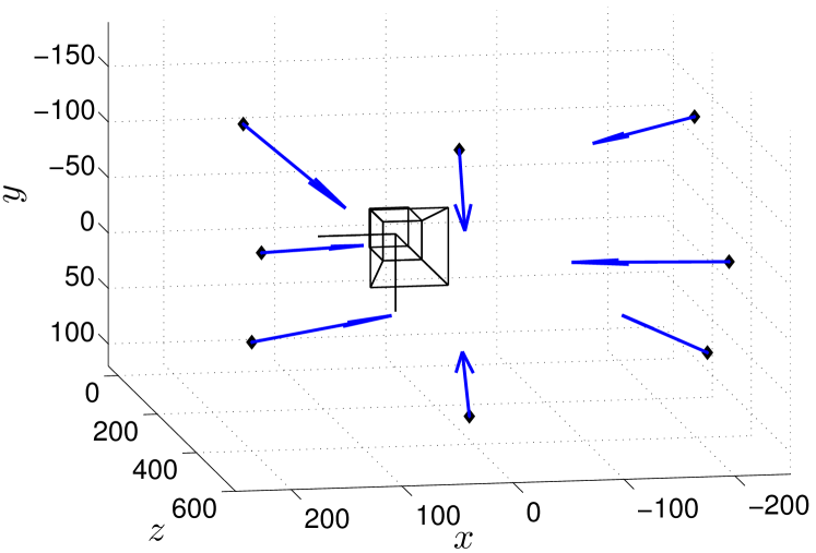
(a)

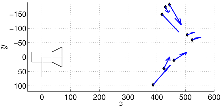
(b)

Figure 5: Two views of a schematic representation of the experimental setup of Fig. 2-a. The camera center is located in $(0,0,0)$. A black marker characterizes the location $\mathbf{x}_{s}$ of each LED (unit $mm$), the orientation of a blue arrow its principal direction $\mathbf{n}_{s}$, and the length of this arrow its intensity $\Phi_{0}$ (up to a common factor).

2.3 Modeling Photometric Stereo with Point Light Sources

If the luminous flux emitted by a LED is described by Model (2.7), then we obtain from (2.13) and (2.14) the following equation for the gray level at pixel $\mathbf{p}$:

$$I(\mathbf{p})=\Psi\,\frac{\rho(\mathbf{p})}{\rho_{0}}\!\left[\frac{\mathbf{n}_{s}\!\cdot\!\left(\!\mathbf{x}\!-\!\mathbf{x}_{s}\!\right)}{\|\mathbf{x}\!-\!\mathbf{x}_{s}\|}\!\right]^{\mu}\frac{\left\{(\mathbf{x}_{s}\!-\!\mathbf{x})\!\cdot\!\mathbf{n}(\mathbf{p})\right\}_{+}}{\|\mathbf{x}_{s}\!-\!\mathbf{x}\|^{3}}.$$ (2.21)

Let us introduce a new definition of the albedo relative to the albedo $\rho_{0}$ of the Lambertian planar calibration pattern:

$$\overline{\rho}(\mathbf{p})=\frac{\rho(\mathbf{p})}{\rho_{0}}.$$ (2.22)

By writing Eq. (2.21) with respect to each LED, and by using Eq. (2.22), we obtain, in each pixel $\mathbf{p}\in\Omega$, the system of equations (2.1), for $i\in\{1,\dots,m\}$.

To solve this system, the introduction of the auxiliary variable $\overline{\mathbf{m}}(\mathbf{p})=\overline{\rho}(\mathbf{p})\,\mathbf{n}(\mathbf{p})$ may seem relevant, since this vector is not constrained to have unit-length, but we will see that this trick loses part of its interest. Defining the following $m$ vectors, $i\in\{1,\dots,m\}$:

$$\mathbf{t}^{i}(\mathbf{x})=\Psi^{i}\left[\frac{\mathbf{n}^{i}_{s}\cdot\left(\mathbf{x}-\mathbf{x}^{i}_{s}\right)}{\|\mathbf{x}-\mathbf{x}^{i}_{s}\|}\right]^{\mu^{i}}\frac{\mathbf{x}^{i}_{s}-\mathbf{x}}{\|\mathbf{x}^{i}_{s}-\mathbf{x}\|^{3}},$$ (2.23)

and neglecting self-shadows ($\{x\}_{+}=x$), then System (2.1) is rewritten in matrix form:

$$\mathbf{I}(\mathbf{p})=\mathbf{T}(\mathbf{x})\,\overline{\mathbf{m}}(\mathbf{p}),$$ (2.24)

where $\mathbf{I}(\mathbf{p})\in\mathbb{R}^{m}$ has been defined in (1.5) and $\mathbf{T}(\mathbf{x})\in\mathbb{R}^{m\times 3}$ is defined as follows:

$$\mathbf{T}(\mathbf{x})=\begin{bmatrix}\mathbf{t}^{1}(\mathbf{x})^{\top}\\ \vdots\\ \mathbf{t}^{m}(\mathbf{x})^{\top}\end{bmatrix}.$$ (2.25)

Eq. (2.24) is similar to (1.4). Knowing the matrix field $\mathbf{T}(\mathbf{x})$ would allow us to estimate its field of pseudo-inverses in order to solve (2.24), just as calculating the pseudo-inverse of $\mathbf{S}$ allows us to solve (1.4). However, the matrix field $\mathbf{T}(\mathbf{x})$ depends on $\mathbf{x}$, and thus on the unknown depth. This simple difference induces major changes when it comes to the numerical solution, as discussed in the next two sections.

3 A Review of Two Variational Approaches for Solving Photometric Stereo under Point Light Source Illumination, with New Insights

In this section, we study two variational approaches from the literature for solving photometric stereo under point light source illumination.

The first one inverts the nonlinear image formation model by recasting it as a sequence of simpler subproblems Ahmad2014 ; Bony2013 ; Collins2012 ; Huang2015 ; Kolagani1992 ; Nie2016b ; Papadhimitri2014b ; Yeh2016 . It consists in estimating the normals and the albedo, assuming that the depth map is fixed, then integrating the normals into a new depth map, and to iterate. We show in Section 3.1 how to improve this standard method in order to estimate absolute depth, without resorting to any prior.

The second approach first linearizes the image formation model by resorting to image ratios, then directly estimates the depth by solving the resulting system of PDEs in an approximate manner Logothetis2017 ; Logothetis_2016 ; Mecca2016 ; CVPR2016 . We show in Section 3.2 that state-of-the-art solutions, which resort to fixed point iterations, may be trapped in local minima. This shortcoming can be avoided by rather using an augmented Lagrangian algorithm.

As in these state-of-the-art methods, self-shadows will be neglected throughougt this section i.e., we abusively assume $\{x\}_{+}=x$. To enforce robustness, we simply follow the approach advocated in Bringier2012 , which systematically eliminates, in each pixel, the highest gray level, which may come from a specular highlight, as well as the two lowest ones, which may correspond to shadows. More elaborate methods for ensuring robustness will be discussed in Section 4.

Apart from robustness issues, we will see that the state-of-the-art methods studied in this section remain unsatisfactory, because their convergence is not established.

3.1 Scheme Inspired by the Classical Numerical Solution of Photometric Stereo

For solving Problem (2.24), it seems quite natural to adapt the solution (1.6) of the linear model (1.4). To linearize (2.24), we have to assume that matrix $\mathbf{T}(\mathbf{x})$ is known. If we proceed iteratively, this can be made possible by replacing, at iteration $(k+1)$, $\mathbf{T}(\mathbf{x})$ by $\mathbf{T}(\mathbf{x}^{(k)})$. This very simple idea has led to several numerical solutions Ahmad2014 ; Bony2013 ; Collins2012 ; Huang2015 ; Kolagani1992 ; Nie2016b ; Papadhimitri2014b ; Yeh2016 , which all require some kind of a priori knowledge on the depth. On the contrary, the scheme we propose here requires none, which constitutes a significant improvement. This new scheme consists in the following algorithm:  

Algorithm 1 (alternating approach)

1:  Initialize $\mathbf{x}^{(0)}$. Set $k:=0$.

2:  loop

3:     Solve Problem (2.24) in the least-squares sense in each $\mathbf{p}\in\Omega$, replacing $\mathbf{T}(\mathbf{x})$ by $\mathbf{T}(\mathbf{x}^{(k)})$, which provides a new estimation of $\overline{\mathbf{m}}(\mathbf{p})$:

$$\overline{\mathbf{m}}^{(k+1)}(\mathbf{p})=\mathbf{T}(\mathbf{x}^{(k)})^{\dagger}\,\mathbf{I}(\mathbf{p}).$$ (3.1)

4:     Deduce a new estimation of the normal $\mathbf{n}(\mathbf{p})$:

$$\mathbf{n}^{(k+1)}(\mathbf{p})=\frac{\overline{\mathbf{m}}^{(k+1)}(\mathbf{p})}{\|\overline{\mathbf{m}}^{(k+1)}(\mathbf{p})\|}.$$ (3.2)

5:     Integrate the new normal field $\mathbf{n}^{(k+1)}$ into an updated 3D-shape $\mathbf{x}^{(k+1)}$, up to a scale factor.

6:     Estimate this scale factor by nonlinear optimization.

7:     Set $k:=k+1$ as long as $k<k_{\text{max}}$.

8:  $\overline{\rho}(\mathbf{p})=\left\|\overline{\mathbf{m}}^{(k_{\text{max}})}(\mathbf{p})\right\|.\lx@algorithmic@hfill\ (3.3)$

For this scheme to be completely specified, we need to set the initial 3D-shape $\mathbf{x}^{(0)}$. We use as initial guess a fronto-parallel plane at distance $z_{0}$ from the camera, $z_{0}$ being a rough estimate of the mean distance from the camera to the scene surface.

Integration of Normals.

Stages 3 and 4 of the scheme above are trivial and can be achieved pixelwise, but Stages 5 and 6 are trickier. From the equalities in (1.1), and by denoting $\nabla z(\mathbf{p})=\left[\partial_{u}z(\mathbf{p}),\partial_{v}z(\mathbf{p})\right]^{\top}$ the gradient of $z$ in $\mathbf{p}$, it is easy to deduce that the (non-unit-length) vector

$$\overline{\mathbf{n}}(\mathbf{p})=\begin{bmatrix}f\,\partial_{u}z(\mathbf{p})\\ f\,\partial_{v}z(\mathbf{p})\\ -z(\mathbf{p})-\mathbf{p}\cdot\nabla z(\mathbf{p})\end{bmatrix}$$ (3.4)

is normal to the surface. Expression (3.4) shows that integrating the (unit-length) normal field $\mathbf{n}$ allows to estimate the depth $z$ only up to a scale factor $\kappa\in\mathbb{R}$, since:

$$\mathbf{n}(\mathbf{p})\propto\begin{bmatrix}f\,\partial_{u}z(\mathbf{p})\\ f\,\partial_{v}z(\mathbf{p})\\ -z(\mathbf{p})\!-\!\mathbf{p}\!\cdot\!\nabla z(\mathbf{p})\end{bmatrix}\propto\begin{bmatrix}f\,\partial_{u}(\kappa\,z)(\mathbf{p})\\ f\,\partial_{v}(\kappa\,z)(\mathbf{p})\\ -(\kappa\,z)(\mathbf{p})\!-\!\mathbf{p}\!\cdot\!\nabla(\kappa\,z)(\mathbf{p})\end{bmatrix}.$$ (3.5)

The collinearity of $\overline{\mathbf{n}}(\mathbf{p})$ and $\mathbf{n}(\mathbf{p})=[n_{1}(\mathbf{p}),n_{2}(\mathbf{p}),n_{3}(\mathbf{p})]^{\top}$ leads to the system

$$\begin{cases}n_{3}(\mathbf{p})\,f\,\partial_{u}z(\mathbf{p})\!+\!n_{1}(\mathbf{p})\left[z(\mathbf{p})\!+\!\mathbf{p}\cdot\!\nabla z(\mathbf{p})\right]=0,\\ n_{3}(\mathbf{p})\,f\,\partial_{v}z(\mathbf{p})\!+\!n_{2}(\mathbf{p})\left[z(\mathbf{p})\!+\!\mathbf{p}\cdot\!\nabla z(\mathbf{p})\right]=0,\end{cases}$$ (3.6)

which is homogeneous in $z(\mathbf{p})$. Introducing the change of variable $\tilde{z}=\log(z)$, which is valid since $z>0$, (3.6) is rewritten

$$\begin{cases}\left[f\,n_{3}(\mathbf{p})+u\,n_{1}(\mathbf{p})\right]\partial_{u}\tilde{z}(\mathbf{p})+v\,n_{1}(\mathbf{p})\partial_{v}\tilde{z}(\mathbf{p})=-n_{1}(\mathbf{p}),\\ u\,n_{2}(\mathbf{p})\partial_{u}\tilde{z}(\mathbf{p})+\left[f\,n_{3}(\mathbf{p})+v\,n_{2}(\mathbf{p})\right]\partial_{v}\tilde{z}(\mathbf{p})=-n_{2}(\mathbf{p}).\end{cases}$$ (3.7)

The determinant of this system is equal to

$$f\,n_{3}(\mathbf{p})\left[u\,n_{1}(\mathbf{p})\!+\!v\,n_{2}(\mathbf{p})\!+\!f\,n_{3}(\mathbf{p})\right]=f\,n_{3}(\mathbf{p})\left[\overline{\mathbf{p}}\cdot\mathbf{n}(\mathbf{p})\right],$$ (3.8)

if we denote

$$\overline{\mathbf{p}}=[u,v,f]^{\top}.$$ (3.9)

It is then easy to deduce the solution of (3.7):

$$\nabla\tilde{z}(\mathbf{p})=-\frac{1}{\overline{\mathbf{p}}\cdot\mathbf{n}(\mathbf{p})}\begin{bmatrix}n_{1}(\mathbf{p})\\ n_{2}(\mathbf{p})\end{bmatrix}.$$ (3.10)

Let us now come back to Stages 5 and 6 of Algorithm 1. The new normal field is $\mathbf{n}^{(k+1)}(\mathbf{p})$, from which we can deduce the gradient $\nabla\tilde{z}^{(k+1)}(\mathbf{p})$ thanks to Eq. (3.10). By integrating this gradient between a pixel $\mathbf{p}_{0}$, chosen arbitrarily inside $\Omega$, and any pixel $\mathbf{p}\in\Omega$, and knowing that $z=\exp\{\tilde{z}\}$, we obtain:

$$z^{(k+1)}(\mathbf{p})\!=\!z^{(k+1)}(\mathbf{p}_{0})\,\exp\!\left\{\!\int_{\mathbf{p}_{0}}^{\mathbf{p}}\!\!\!\!\nabla\tilde{z}^{(k+1)}(\mathbf{q})\cdot\mathrm{d}\mathbf{q}\!\right\}.$$ (3.11)

This integral can be calculated along one single path inside $\Omega$ going from $\mathbf{p}_{0}$ to $\mathbf{p}$, but since the gradient field $\nabla\tilde{z}^{(k+1)}(\mathbf{p})$ is never rigorously integrable in practice, this calculus usually depends on the choice of the path Wu1988 . The most common parry to this well-known problem consists in resorting to a variational approach, see for instance Durou2016 for some discussion.

Expression (3.11) confirms that the depth can only be calculated, from $\mathbf{n}^{(k+1)}(\mathbf{p})$, up to a scale factor equal to $z^{(k+1)}(\mathbf{p}_{0})$. Let us determine this scale factor by minimization of the reprojection error of Model (2.24) over the entire domain $\Omega$. Knowing that, from (1.1) and (3.9), we get $\mathbf{x}=\frac{z}{f}\,\overline{\mathbf{p}}$, this comes down to solving the following nonlinear least-squares problem:

$$z^{(k+1)}(\mathbf{p}_{0})=\underset{w\,\in\,\mathbb{R}^{+}}{\arg\min~{}}\mathcal{E}_{\mathrm{alt}}(w):=\sum_{\mathbf{p}\in\Omega}\Big{\|}\mathbf{I}(\mathbf{p})$$

$$\quad-\!\mathbf{T}\Big{(}\frac{w}{f}\exp\left\{\int_{\mathbf{p}_{0}}^{\mathbf{p}}\nabla\tilde{z}^{(k+1)}(\mathbf{q})\cdot\mathrm{d}\mathbf{q}\right\}\overline{\mathbf{p}}\Big{)}\,\overline{\mathbf{m}}^{(k+1)}(\mathbf{p})\Big{\|}^{2},$$ (3.12)

which allows us to eventually write the 3D-shape update (Stages 5 and 6):

$$\mathbf{x}^{(k+1)}\!=\!\frac{z^{(k+1)}(\mathbf{p}_{0})}{f}\,\exp\!\left\{\!\int_{\mathbf{p}_{0}}^{\mathbf{p}}\!\!\!\!\nabla\tilde{z}^{(k+1)}(\mathbf{q})\cdot\mathrm{d}\mathbf{q}\!\right\}\overline{\mathbf{p}}.$$ (3.13)

Experimental Validation.

Despite the lack of theoretical guarantee, convergence of this scheme is empirically observed, provided that the initial 3D-shape $\mathbf{x}^{(0)}$ is not too distant from the scene surface. For the curves in Fig. 6, several fronto-parallel planes with equation $z\equiv z_{0}$ were tested as initial guess. The mean distance from the camera to the scene being approximately $700~{}mm$, it is not surprising that the fastest convergence is observed for this value of $z_{0}$. Besides, this graph also shows that under-estimating the initial scale quite a lot is not a problem, whereas over-estimating it severely slows down the process.

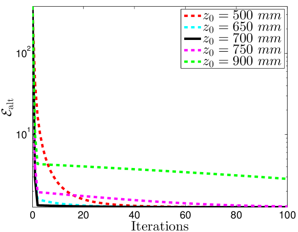
Figure 6: Evolution of the energy $\mathcal{E}_{\mathrm{alt}}$ of the alternating approach, defined in (3.12), in function of the iterations, when the initial 3D-shape is a fronto-parallel plane with equation $z\equiv z_{0}$. The used data are the $m=8$ images of the plaster statuette of Fig. 2. The proposed scheme consists in alternating normal estimation, normal integration and scale estimation (cf. Algorithm 1). It converges towards the same solution (at different speeds), for the five tested values of $z_{0}$.

Fig. 7 allows to compare the 3D-shape obtained by photometric stereo, from sub-images of size $920\times 1178$ in full resolution (bounding box of the statuette), which contain $773794$ pixels inside $\Omega$, with the ground truth obtained by laser scanning, which contains $1753010$ points. The points density is thus almost the same on the front of the statuette, since we did not reconstruct its back. However, our result is achieved in less than ten seconds (five iterations of a Matlab code on a recent i7 processor), instead of several hours for the ground truth, while we also estimate the albedo.

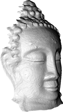
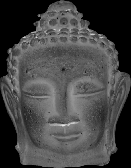
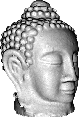
(a)	(b)	(c)

Figure 7: (a) 3D-reconstruction and (b) albedo obtained with Algorithm 1. (c) Ground truth 3D-shape obtained by laser scanning. Photometric stereo not only provides a 3D-shape qualitatively similar to the laser scan, but also provides the albedo.

(a)

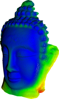
(b)

Figure 8: (a) Histogram of point-to-point distances between the alternating 3D-reconstruction and the ground truth (cf. Fig. 7). The median value is $1.3~{}mm$. (b) Spatial distribution of these distances. The histogram peak is not located in zero. As we will see in Section 3.2, this bias can be avoided by resorting to a differential approach based on PDEs.

Fig. 8-a shows the histogram of point-to-point distances between our result (Fig. 7-a) and the ground truth (Fig. 7-c). The median value is $1.3~{}mm$. The spatial distribution of these distances (Fig. 8-b), shows that the largest distances are observed on the highest slopes of the surface. This clearly comes from the facts that, even for a diffuse material such as plaster, the Lambertian model is not valid under skimming lighting, and that self-shadows were neglected.

More realistic reflectance models, such as the one proposed by Oren and Nayar in Oren1995 , would perhaps improve accuracy of the 3D-reconstruction in such points, and we will see in Section 4 how to handle self-shadows. But, as we shall see now, bias also comes from normal integration. In the next section, we describe a different formulation of photometric stereo which permits to avoid integration, by solving a system of PDEs in $z$.

3.2 Direct Depth Estimation using Image Ratios

The scheme proposed in Section 3.1 suffers from several defects. It requires to integrate the gradient $\nabla\tilde{z}^{(k+1)}(\mathbf{p})$ at each iteration. This is not achieved by the naive formulation (3.12), but using more sophisticated methods which allow to overcome the problem of non-integrability Durou2009 . Still, bias due to inaccurate normal estimation should not have to be corrected during integration. Instead, it seems more justified to directly estimate the depth map, without resorting to intermediate normal estimation. This can be achieved by recasting photometric stereo as a system of quasilinear PDEs.

Differential Reformulation of Problem (2.24).

Let us recall (cf. Eq. (1.1)) that the coordinates of the 3D-point $\mathbf{x}$ conjugate to a pixel $\mathbf{p}$ are completely characterized by the depth $z(\mathbf{p})$:

$$\mathbf{x}=\frac{z(\mathbf{p})}{f}\,\begin{bmatrix}\mathbf{p}\\ f\end{bmatrix}.$$ (3.14)

The vectors $\mathbf{t}^{i}(\mathbf{x})$ defined in (2.23) thus depend on the unknown depth values $z(\mathbf{p})$. Using once again the change of variable $\tilde{z}=\log(z)$, we consider from now on each $\mathbf{t}^{i}$, $i\in\{1,\dots,m\}$, as a vector field depending on the unknown map $\tilde{z}$:

$$\begin{array}[]{rccl}\mathbf{t}^{i}(\tilde{z}):&\Omega&\to&\mathbb{R}^{3}\\[-5.0pt] &\mathbf{p}&\mapsto&\mathbf{t}^{i}(\tilde{z})(\mathbf{p})=\Psi^{i}\left[-\frac{\mathbf{n}_{s}^{i}\cdot\mathbf{v}^{i}(\tilde{z})(\mathbf{p})}{\|\mathbf{v}^{i}(\tilde{z})(\mathbf{p})\|}\right]^{\mu^{i}}\frac{\mathbf{v}^{i}(\tilde{z})(\mathbf{p})}{\|\mathbf{v}^{i}(\tilde{z})(\mathbf{p})\|^{3}},\end{array}$$ (3.15)

where each field $\mathbf{t}^{i}(\tilde{z})$ depends in a nonlinear way on the unknown (log-) depth map $\tilde{z}$, through the following vector field:

$$\begin{array}[]{rccl}\mathbf{v}^{i}(\tilde{z}):&\Omega&\to&\mathbb{R}^{3}\\[-5.0pt] &\mathbf{p}&\mapsto&\mathbf{v}^{i}(\tilde{z})(\mathbf{p})=\mathbf{x}^{i}_{s}-\frac{\exp\left(\tilde{z}(\mathbf{p})\right)}{f}\,\begin{bmatrix}\mathbf{p}\\ f\end{bmatrix}.\end{array}$$ (3.16)

Knowing that the (non-unit-length) vector $\overline{\mathbf{n}}(\mathbf{p})$ defined in (3.4), divided by $z(\mathbf{p})$, is normal to the surface, and still neglecting self-shadows, we can rewrite System (2.1), in each pixel $\mathbf{p}\in\Omega$:

$$I^{i}(\mathbf{p})=\frac{\overline{\rho}(\mathbf{p})}{d(\tilde{z})(\mathbf{p})}\,\mathbf{t}^{i}(\tilde{z})(\mathbf{p})\cdot\begin{bmatrix}f\nabla\tilde{z}(\mathbf{p})\\ -1-\mathbf{p}\cdotp\nabla\tilde{z}(\mathbf{p})\end{bmatrix},$$

$$\qquad\qquad\qquad\qquad\qquad\qquad\qquad~{}i\in\{1,\dots,m\},$$ (3.17)

with

$$d(\tilde{z})(\mathbf{p})=\sqrt{f^{2}\left\|\nabla\tilde{z}(\mathbf{p})\right\|^{2}+\left(-1-\mathbf{p}\cdotp\nabla\tilde{z}(\mathbf{p})\right)^{2}}.$$ (3.18)

Partial Linearization of (3.17) using Image Ratios.

In comparison with Eqs. (2.1), the PDEs (3.17) explicitly depend on the unknown map $\tilde{z}$, and thus remove the need for alternating normal estimation and integration. However, these equations contain two difficulties: they are nonlinear and cannot be solved locally. We can eliminate the nonlinearity due to the coefficient of normalization $d(\tilde{z})(\mathbf{p})$. Indeed, neither the relative albedo $\overline{\rho}(\mathbf{p})$, nor this coefficient, depend on the index $i$ of the LED. We deduce from any pair $\{i,j\}\in\{1,\dots,m\}^{2}$, $i\neq j$, of equations from (3.17), the following equalities:

$$\frac{\overline{\rho}(\mathbf{p})}{d(\tilde{z})(\mathbf{p})} =\frac{I^{i}(\mathbf{p})}{\mathbf{a}^{i}(\tilde{z})(\mathbf{p})\cdot\nabla\tilde{z}(\mathbf{p})-b^{i}(\tilde{z})(\mathbf{p})}$$

$$=\frac{I^{j}(\mathbf{p})}{\mathbf{a}^{j}(\tilde{z})(\mathbf{p})\cdot\nabla\tilde{z}(\mathbf{p})-b^{j}(\tilde{z})(\mathbf{p})},$$ (3.19)

with the following definitions of $\mathbf{a}^{i}(\tilde{z})(\mathbf{p})$ and $b^{i}(\tilde{z})(\mathbf{p})$, denoting $\mathbf{t}^{i}(\tilde{z})(\mathbf{p})=[t^{i}_{1}(\tilde{z})(\mathbf{p}),t^{i}_{2}(\tilde{z})(\mathbf{p}),t^{i}_{3}(\tilde{z})(\mathbf{p})]^{\top}$:

$$\mathbf{a}^{i}(\tilde{z})(\mathbf{p}) =f\begin{bmatrix}t^{i}_{1}(\tilde{z})(\mathbf{p})\\ t^{i}_{2}(\tilde{z})(\mathbf{p})\end{bmatrix}-t^{i}_{3}(\tilde{z})(\mathbf{p})\,\mathbf{p},$$ (3.20)

$$b^{i}(\tilde{z})(\mathbf{p}) =t^{i}_{3}(\tilde{z})(\mathbf{p}).$$ (3.21)

From the equalities (3.19), we obtain:

$$\underbrace{\begin{bmatrix}I^{i}(\mathbf{p})\,\mathbf{a}^{j}(\tilde{z})(\mathbf{p})-I^{j}(\mathbf{p})\,\mathbf{a}^{i}(\tilde{z})(\mathbf{p})\end{bmatrix}}_{\mathbf{a}^{i,j}(\tilde{z})(\mathbf{p})}\cdot\,\nabla\tilde{z}(\mathbf{p})$$

$$\qquad=\underbrace{\left[I^{i}(\mathbf{p})\,b^{j}(\tilde{z})(\mathbf{p})-I^{j}(\mathbf{p})\,b^{i}(\tilde{z})(\mathbf{p})\right]}_{b^{i,j}(\tilde{z})(\mathbf{p})}.$$ (3.22)

The fields $\mathbf{a}^{i,j}(\tilde{z})$ and $b^{i,j}(\tilde{z})$ defined in (3.22) depend on $\tilde{z}$ but not on $\nabla\tilde{z}$: Eq. (3.22) is thus a quasi-linear PDE in $z$ over $\Omega$. It could be solved by the characteristic strips expansion method Mecca2015 ; Mecca2014b if we were dealing with $m=2$ images only, but using a larger number of images is necessary in order to design a robust 3D-reconstruction method. Since we are provided with $m>2$ images, we follow Gotardo2015 ; Logothetis2017 ; Logothetis_2016 ; Mecca2016 ; CVPR2016 ; Smith2016 and write $\binom{m}{2}$ PDEs such as (3.22) formed by the $\binom{m}{2}$ pairs $\{i,j\}\in\{1,\dots,m\}^{2}$, $i\neq j$. Forming the matrix field $\mathbf{A}(\tilde{z}):\,\Omega\to\mathbb{R}^{\binom{m}{2}\times 2}$ by concatenation of the row vectors $\mathbf{a}^{i,j}(\tilde{z})(\mathbf{p})^{\top}$, and the vector field $\mathbf{b}(\tilde{z}):\,\Omega\to\mathbb{R}^{\binom{m}{2}}$ by concatenation of the scalar values $b^{i,j}(\tilde{z})(\mathbf{p})$, the system of PDEs to solve is written:

$$\mathbf{A}(\tilde{z})\,\nabla\tilde{z}=\mathbf{b}(\tilde{z})\quad\text{over~{}}\Omega.$$ (3.23)

This new differential formulation of photometric stereo seems simpler than the original differential formulation (3.17), since the main source of nonlinearity, due to the denominator $d(\tilde{z})(\mathbf{p})$, has been eliminated. However, it still presents two difficulties. First, the PDEs (3.23) are generally incompatible and hence do not admit an exact solution. It is thus necessary to estimate an approximate one, by resorting to a variational approach. Assuming that each of the $\binom{m}{2}$ equalities in System (3.23) is satisfied up to an additive, zero-mean, Gaussian noise, one should estimate such a solution by solving the following variational problem:

$$\underset{\tilde{z}:\Omega\rightarrow\mathbb{R}}{\min~{}}\,\mathcal{E}_{\mathrm{rat}}(\tilde{z}):=\|\mathbf{A}(\tilde{z})\,\nabla\tilde{z}-\mathbf{b}(\tilde{z})\|_{L^{2}(\Omega)}^{2}.$$ (3.24)

Second, the PDEs (3.22) do not allow to estimate the scale of the scene. Indeed, when all the depth values simultaneously tend to infinity, then both members of (3.22) tend to zero (because the coordinates of $\mathbf{t}^{i}$ do so, cf. (3.15)). Thus, a large, distant 3D-shape will always “better” fit these PDEs (in the sense of the criterion $\mathcal{E}_{\mathrm{rat}}$ defined in Eq. (3.24)) than a small, nearby one (cf. Figs. 10 and 11). A “locally optimal” solution close to a very good initial estimate should thus be sought.

Fixed Point Iterations for Solving (3.24).

It has been proposed in Logothetis2017 ; Logothetis_2016 ; Mecca2016 ; CVPR2016 to iteratively estimate a solution of Problem (3.24), by uncoupling the (linear) estimation of $\tilde{z}$ from the (nonlinear) estimations of $\mathbf{A}(\tilde{z})$ and of $\mathbf{b}(\tilde{z})$. This can be achieved by rewriting (3.24) as the following constrained optimization problem:

$$\begin{array}[]{l}\underset{\tilde{z}:\Omega\rightarrow\mathbb{R}}{\min~{}}\,\|\mathbf{A}\,\nabla\tilde{z}-\mathbf{b}\|_{L^{2}(\Omega)}^{2}\\ \text{s.t.~{}}\begin{cases}\mathbf{A}&\!\!\!=\mathbf{A}(\tilde{z}),\\ \mathbf{b}&\!\!\!=\mathbf{b}(\tilde{z}),\end{cases}\end{array}$$ (3.25)

and resorting to a fixed point iterative scheme:

$$\tilde{z}^{(k+1)}= ~{}\underset{\tilde{z}:\Omega\rightarrow\mathbb{R}}{\arg\min~{}}\|\mathbf{A}^{(k)}\,\nabla\tilde{z}-\mathbf{b}^{(k)}\|_{L^{2}(\Omega)}^{2},$$ (3.26)

$$\mathbf{A}^{(k+1)}= ~{}\mathbf{A}(\tilde{z}^{(k+1)}),$$ (3.27)

$$\mathbf{b}^{(k+1)}= ~{}\mathbf{b}(\tilde{z}^{(k+1)}).$$ (3.28)

In the linear least-squares variational problem (3.26), the solution can be computed only up to an additive constant. Therefore, the matrix of the system arising from the normal equations associated to the discretized problem will be symmetric, positive, but rank-1 deficient, and thus only semi-definite. Fig. 9 shows that this may cause the fixed point scheme not to decrease the energy after each iteration. This issue can be resolved by resorting to the alternating direction method of multipliers (ADMM algorithm), a standard procedure which dates back to the 70’s GabayMercier1976 ; Glowinski1975 , but has been revisited recently Boyd2011 .

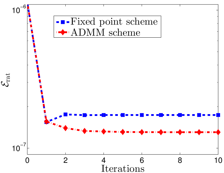
Figure 9: Evolution of the energy $\mathcal{E}_{\mathrm{rat}}$ of the ratio-based approach, defined in (3.24), in function of the iterations, for the data of Fig. 2 (the initial 3D-shape is a fronto-parallel plane with equation $z\equiv 700~{}mm$). With the fixed point scheme, the energy is not always decreased after each iteration, contrarily to the ADMM scheme we are going to introduce.

ADMM Iterations for Solving (3.24).

Instead of “freezing” the nonlinearities of the variational problem (3.24), $\tilde{z}$ can be estimated not only from the linearized parts, but also from the nonlinear ones. In this view, we introduce an auxiliary variable $\overline{z}$ and reformulate Problem (3.24) as follows:

$$\begin{array}[]{rl}&\underset{\overline{z},\tilde{z}}{\min}\left\|\mathbf{A}(\overline{z})\,\nabla\tilde{z}-\mathbf{b}(\overline{z})\right\|_{L^{2}(\Omega)}^{2}\\ &\text{s.t.~{}}\tilde{z}=\overline{z}.\end{array}$$ (3.29)

In order to solve the constrained optimization problem (3.29), let us introduce a dual variable $h$ and a descent step $\nu$. A local solution of (3.29) is then obtained at convergence of the following algorithm:

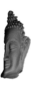
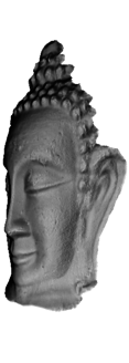
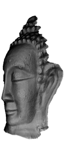
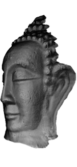
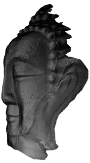
(a) $z_{0}=500~{}mm$	(b) $z_{0}=650~{}mm$	(c) $z_{0}=700~{}mm$	(d) $z_{0}=750~{}mm$	(e) $z_{0}=900~{}mm$

Figure 10: 3D-reconstructions after 10 iterations of the ADMM scheme, taking as initial guess different fronto-parallel planes $z\equiv z_{0}$. The median of the distances to ground truth is, from left to right: $3.05~{}mm$, $2.88~{}mm$, $1.68~{}mm$, $2.08~{}mm$ and $5.86~{}mm$. When the initial guess is too close to the camera, the 3D-reconstruction is flattened, while the scale is overestimated when starting too far away from the camera (although this yields a lower energy, see Fig. 11).

Algorithm 2 (ratio-based ADMM approach)

1:  Initialize $\tilde{z}^{(0)}=\overline{z}^{(0)}$, $h^{(0)}\equiv 0$. Set $k:=0$.

2:  loop

3:     Update $\tilde{z}$ by using the linear part, “while keeping $\tilde{z}$ close to $\overline{z}^{(k)}$”:

$$\tilde{z}^{(k+1)} =\underset{\tilde{z}}{\arg\min}\left\|\mathbf{A}(\overline{z}^{(k)})\nabla\tilde{z}-\mathbf{b}(\overline{z}^{(k)})\right\|_{L^{2}(\Omega)}^{2}$$

$$\qquad+\frac{1}{2\,\nu}\left\|\tilde{z}-\overline{z}^{(k)}+h^{(k)}\right\|_{L^{2}(\Omega)}^{2}.$$ (3.30)

4:     Update $\overline{z}$ by using the nonlinear part, “while keeping $\overline{z}$ close to $\tilde{z}^{(k+1)}$”:

$${\overline{z}}^{(k+1)} =\underset{\overline{z}}{\arg\min}\left\|\mathbf{A}(\overline{z})\,\nabla\tilde{z}^{(k+1)}-\mathbf{b}(\overline{z})\right\|_{L^{2}(\Omega)}^{2}$$

$$\qquad+\frac{1}{2\,\nu}\left\|\tilde{z}^{(k+1)}\!\!-\!\overline{z}\!+\!h^{(k)}\right\|_{L^{2}(\Omega)}^{2}.$$ (3.31)

5:     Update the dual variable $h$:

$$h^{(k+1)}=h^{(k)}+\tilde{z}^{(k+1)}-\overline{z}^{(k+1)}.$$ (3.32)

6:     If the stopping criterion is not satisfied, then set $k:=k+1$.

Stage (3.30) of Algorithm 2 is a linear least-squares problem which can be solved using the normal equations of its discrete formulation. The presence of the regularization term now guarantees the positive definiteness of the matrix of the system. This matrix is however too large to be inverted directly. Therefore, we resort to the conjugate gradient algorithm.

Thanks to the auxiliary variable $\overline{z}$, which decouples $\nabla\tilde{z}$ and $\tilde{z}$ in Problem (3.29), Stage (3.31) of Algorithm 2 is a local nonlinear least-squares problem: in fact, $\nabla\overline{z}$ is not involved in this problem, which can be solved pixelwise. Problem (3.31) thus reduces to a nonlinear least-squares estimation problem of one real variable, which can be solved by a standard method such as the Levenberg-Marquardt algorithm.

Because of the nonlinearity of Problem (3.31), it is unfortunately impossible to guarantee convergence for this ADMM scheme, which depends on the initialization and on parameter $\nu$ Boyd2011 . A reasonable initialization strategy consists in using the solution provided by Algorithm 1 (cf. Section 3.1). As for the descent step $\nu$, we iteratively calculate its optimal value according to the Penalty Varying Parameter procedure described in Boyd2011 . Finally, the iterations stop when the relative variation of the criterion of Problem (3.24) falls under a threshold equal to $10^{-4}$.

Fig. 9 shows that with such choices, Problem (3.24) is solved more efficiently than with the fixed point scheme: the energy is now decreased at each iteration. Fig. 11 shows that this is the case whatever the initial guess, although initialization has a strong impact on the solution, as confirmed by Fig. 10.

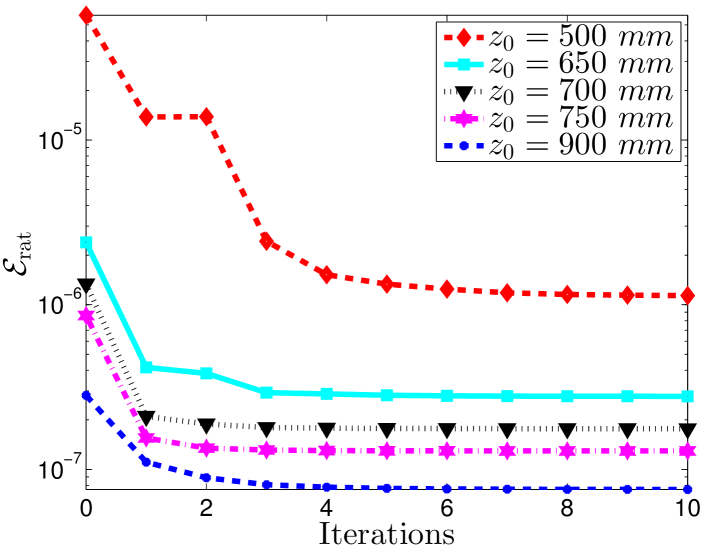
Figure 11: Evolution of the energy $\mathcal{E}_{\mathrm{rat}}$ defined in (3.24), in function of the iterations, for the data of Fig. 2. Using as initialization $\tilde{z}^{(0)}\equiv\log(z_{0})$, the ADMM scheme always converges towards a local minimum, yet this minimum strongly depends on the value of $z_{0}$. Besides, a lower final energy does not necessarily means a better 3D-reconstruction, as shown in Fig. 10. Hence, not only a careful initial guess is of primary importance, but the criterion derived from image ratios prevents automatic scale estimation.

Fig. 12 shows the 3D-reconstruction obtained by refining the results of Section 3.1 using Algorithm 2. At first sight, the 3D-shape depicted in Fig. 12-a seems hardly different from that of Fig. 7-a, but the comparison of histograms in Figs. 8-a and 12-b indicates that bias has been significantly reduced. This shows the superiority of direct depth estimation over alternating normal estimation and integration.

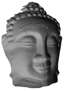
(a)

(b)

Figure 12: (a) 3D-reconstruction obtained with Algorithm 2, using the result from Fig. 7-a as initial guess. (b) Histogram of point-to-point distances between this 3D-shape and the ground truth (cf. Fig. 7-c). The median value is $1.2~{}mm$.

However, the lack of convergence guarantees and the strong dependency on the initialization remain limiting bottlenecks. The method discussed in the next section overcomes both these issues.

4 A New, Provably Convergent Variational Approach for Photometric Stereo under Point Light Source Illumination

When it comes to solving photometric stereo under point light source illumination, there are two main difficulties: the dependency of the lighting vectors on the depth map (cf. Eq. (3.15)), and the presence of the nonlinear coefficient ensuring that the normal vectors have unit-length (cf. Eq. (3.18)).

The alternating strategy from Section 3.1 solves the former issue by freezing the lighting vectors at each iteration, and the latter by simultaneously estimating the normal vector and the albedo. The objective function tackled in this approach, which is based on the reprojection error, seems to be the most relevant. Indeed, the final result seems to be independent from the initialization, although convergence is not established.

On the other hand, the differential strategy from Section 3.2 explicitly tackles the nonlinear dependency of lighting on the depth, and eliminates the other nonlinearity using image ratios. Directly estimating depth reduces bias, but the objective function derived from image ratios admits a global solution which is not acceptable (depth uniformly tending to $+\infty$), albedo is not estimated and convergence is not established either.

Therefore, an ideal numerical solution should: ($i$) build upon a differential approach, in order to reduce bias, ($ii$) avoid linearization using ratios, in order to avoid the trivial solution and allow albedo estimation, and ($iii$) be provably convergent. The variational approach presented in this section, initially presented in SSVM2017 , satisfies these three criteria.

4.1 Proposed Discrete Variational Framework

The nonlinearity of the PDEs (3.17) with respect to $\nabla\tilde{z}$, due to the nonlinear dependency of $d(\tilde{z})$ (see Eq. (3.18)), is challenging. We could explicitly consider this nonlinear coefficient within a variational framework Hoeltgen_2016 , but we rather take inspiration from the way conventional photometric stereo Woodham1980a is linearized and integrate the nonlinearity inside the albedo variable, as we proposed recently in SSVM2017 ; CVPR2017 . Instead of estimating $\overline{\rho}(\mathbf{p})$ in each pixel $\mathbf{p}$, we thus rather estimate:

$$\tilde{\rho}(\mathbf{p})=\frac{\overline{\rho}(\mathbf{p})}{d(\tilde{z})(\mathbf{p})}.$$ (4.1)

The system of PDEs (3.17) is then rewritten as

$$I^{i}(\mathbf{p})=\tilde{\rho}(\mathbf{p})\,\left[\mathbf{Q}(\mathbf{p})\,\mathbf{t}^{i}(\tilde{z})(\mathbf{p})\right]\cdot\begin{bmatrix}\nabla\tilde{z}(\mathbf{p})\\ -1\end{bmatrix},$$

$$\qquad\qquad\qquad\qquad\qquad\qquad\qquad~{}i\in\{1,\dots,m\},$$ (4.2)

where we use the following notation, $\forall\mathbf{p}=\left[u,v\right]^{\top}\in\Omega$:

$$\mathbf{Q}(\mathbf{p})= \begin{bmatrix}f&0&-u\\ 0&f&-v\\ 0&0&1\end{bmatrix}.$$ (4.3)

System (4.2) is a system of quasilinear PDEs in $(\tilde{\rho},\tilde{z})$, because $\mathbf{t}^{i}(\tilde{z})$ only depends on $\tilde{z}$, and not on $\nabla\tilde{z}$. Once $\tilde{\rho}$ and $\tilde{z}$ are estimated, it is straightforward to recover the “real” albedo $\overline{\rho}$ using (4.1).

Let us now denote $j\in\{1,\dots,n\}$ the indices of the pixels inside $\Omega$, $I^{i}_{j}$ the gray level of pixel $j$ in image $I^{i}$, $\tilde{\bm{\rho}}\in\mathbb{R}^{n}$ and $\tilde{\mathbf{z}}\in\mathbb{R}^{n}$ the vectors stacking the unknown values $\tilde{\rho}_{j}$ and $\tilde{z}_{j}$, $\mathbf{t}^{i}_{j}(\tilde{z}_{j})\in\mathbb{R}^{3}$ the vector $\mathbf{t}^{i}(\tilde{z})$ at pixel $j$, which smoothly (though nonlinearly) depends on $\tilde{z}_{j}$, and $\mathbf{Q}_{j}$ the matrix defined in Eq. (4.3) at pixel $j$. Then, the discrete counterpart of System (4.2) is written as the following system of nonlinear equations in $(\tilde{\bm{\rho}},\tilde{\mathbf{z}})$:

$$I^{i}_{j}=\tilde{\rho}_{j}\,\left[\mathbf{Q}_{j}\,\mathbf{t}^{i}_{j}(\tilde{z}_{j})\right]\cdot\begin{bmatrix}\left(\nabla\mathbf{\tilde{z}}\right)_{j}\\ -1\end{bmatrix},$$

$$\qquad\qquad\qquad\qquad i\in\{1,\dots,m\},\,j\in\{1,\dots,n\},$$ (4.4)

where $\left(\nabla\tilde{\mathbf{z}}\right)_{j}\in\mathbb{R}^{2}$ represents a finite differences approximation of the gradient of $\tilde{z}$ at pixel $j$.

Our goal is to jointly estimate $\tilde{\bm{\rho}}\in\mathbb{R}^{n}$ and $\tilde{\bm{z}}\in\mathbb{R}^{n}$ from the set of nonlinear equations (4.4), as solution of the following discrete optimization problem:

$$\min_{\begin{subarray}{c}\tilde{\bm{\rho}},\tilde{\bm{z}}\end{subarray}}\mathcal{E}(\tilde{\bm{\rho}},\tilde{\bm{z}}):=\sum_{j=1}^{n}\sum_{i=1}^{m}\phi\left(r^{i}_{j}(\tilde{\bm{\rho}},\tilde{\bm{z}})\right),$$ (4.5)

where the residual $r^{i}_{j}(\tilde{\bm{\rho}},\tilde{\bm{z}})$ depends locally (and linearly) on $\tilde{\bm{\rho}}$, but globally (and nonlinearly) on $\tilde{\bm{z}}$:

$$r^{i}_{j}(\tilde{\bm{\rho}},\tilde{\bm{z}})=\tilde{\rho}_{j}\left\{\zeta^{i}_{j}(\tilde{\bm{z}})\right\}_{+}-I^{i}_{j},$$ (4.6)

with

$$\zeta^{i}_{j}(\tilde{\bm{z}})=\left[\mathbf{Q}_{j}\mathbf{t}^{i}_{j}(\tilde{z}_{j})\right]\cdot\begin{bmatrix}(\nabla\tilde{\bm{z}})_{j}\\ -1\end{bmatrix}.$$ (4.7)

An advantage of our formulation is to be generic i.e., independent from the choice of the operator $\{\cdotp\}_{+}$ and of the function $\phi$. For fair comparison with the algorithms in Section 3, one can use $\{x\}_{+}=x$ and $\phi(x)=\phi_{\text{LS}}(x)=x^{2}$. To improve robustness, self-shadows can be explicitly handled by using $\{x\}_{+}=\max\{x,0\}$, and the estimator $\phi$ can be chosen as any $\mathbb{R}\to\mathbb{R}^{+}$ function which is even, twice continuously differentiable, and monotonically increasing over $\mathbb{R}^{+}$ such that:

$$\frac{\phi^{\prime}(x)}{x}\geq\phi^{\prime\prime}(x),~{}\forall x\in\mathbb{R}.$$ (4.8)

A typical example is Cauchy’s robust M-estimator:

$$\phi_{\text{Cauchy}}(x)=\lambda^{2}\log\left(1+\frac{x^{2}}{\lambda^{2}}\right),$$ (4.9)

where the parameter $\lambda$ is user-defined (we use $\lambda=0.1$).

4.2 Alternating Reweighted Least-Squares for Solving (4.5)

Our goal is to find a local minimizer $(\tilde{\bm{\rho}}^{*},\tilde{\bm{z}}^{*})$ for (4.5), which must satisfy the following first-order conditions:

$$\frac{\partial\mathcal{E}}{\partial\tilde{\bm{\rho}}}(\tilde{\bm{\rho}}^{*}\!,\!\tilde{\bm{z}}^{*}) \!=\!\!\sum_{j=1}^{n}\!\sum_{i=1}^{m}\!\phi^{\prime}(r^{i}_{j}(\tilde{\bm{\rho}}^{*}\!,\tilde{\bm{z}}^{*}))\frac{\partial r^{i}_{j}}{\partial\tilde{\bm{\rho}}}(\tilde{\bm{\rho}}^{*}\!,\tilde{\bm{z}}^{*}\!)\!=\!{\bm{0}},$$ (4.10)

$$\frac{\partial\mathcal{E}}{\partial\tilde{\bm{z}}}(\tilde{\bm{\rho}}^{*}\!,\!\tilde{\bm{z}}^{*}) \!=\!\!\sum_{j=1}^{n}\!\sum_{i=1}^{m}\!\phi^{\prime}(r^{i}_{j}(\tilde{\bm{\rho}}^{*}\!,\tilde{\bm{z}}^{*}))\frac{\partial r^{i}_{j}}{\partial\tilde{\bm{z}}}(\tilde{\bm{\rho}}^{*}\!,\tilde{\bm{z}}^{*}\!)\!=\!{\bm{0}},$$ (4.11)

with:

$$\frac{\partial r^{i}_{j}}{\partial\tilde{\rho}_{l}}(\tilde{\bm{\rho}}^{*},\tilde{\bm{z}}^{*}) =\begin{cases}\{\zeta^{i}_{j}(\tilde{\bm{z}}^{*})\}_{+}&\text{~{}if~{}}l=j,\\ 0&\text{~{}if~{}}l\neq j,\\ \end{cases}$$ (4.12)

$$\frac{\partial r^{i}_{j}}{\partial\tilde{\bm{z}}}(\tilde{\bm{\rho}}^{*},\tilde{\bm{z}}^{*}) =\tilde{\rho}^{*}_{j}\,\chi(\zeta^{i}_{j}(\tilde{\bm{z}}^{*}))\,\partial\zeta^{i}_{j}(\tilde{\bm{z}}^{*}).$$ (4.13)

In (4.13), $\chi$ is the (sub-)derivative of $\{\cdotp\}_{+}$, which is a constant function equal to $1$ if $\{x\}_{+}=x$, and the Heaviside function if $\{x\}_{+}=\max\{x,0\}$.

For this purpose, we derive an alternating reweighted least-squares (ARLS) scheme. Suggested by its name, the ARLS scheme alternates Newton-like steps over $\tilde{\bm{\rho}}$ and $\tilde{\bm{z}}$, which can be interpreted as iteratively reweighted least-squares iterations. Similar to the famous iteratively reweighted least-squares Wolke1988 (IRLS) algorithm, ARLS solves the original (possibly non-convex) problem (4.5) iteratively, by recasting it as a series of simpler quadratic programs.

Given the current estimate $(\tilde{\bm{\rho}}^{(k)},\tilde{\bm{z}}^{(k)})$ of the solution, ARLS first freezes $\tilde{\bm{z}}$ and updates $\tilde{\bm{\rho}}$ by minimizing the following local quadratic approximation of $\mathcal{E}(\cdot,\tilde{\bm{z}}^{(k)})$ around $\tilde{\bm{\rho}}^{(k)}$:

$$\mathcal{E}(\cdot,\tilde{\bm{z}}^{(k)})\approx\sum_{j=1}^{n}\sum_{i=1}^{m}\Bigg{\{}\phi\left(r^{i}_{j}(\tilde{\bm{\rho}}^{(k)},\tilde{\bm{z}}^{(k)})\right)$$

$$\quad+\frac{\phi^{\prime}(r^{i}_{j}(\tilde{\bm{\rho}}^{(k)},\tilde{\bm{z}}^{(k)}))}{r^{i}_{j}(\tilde{\bm{\rho}}^{(k)},\tilde{\bm{z}}^{(k)})}\,\frac{r^{i}_{j}(\cdot,\tilde{\bm{z}}^{(k)})^{2}-r^{i}_{j}(\tilde{\bm{\rho}}^{(k)},\tilde{\bm{z}}^{(k)})^{2}}{2}\Bigg{\}},$$ (4.14)

where we set $\frac{\phi^{\prime}(r^{i}_{j}(\tilde{\bm{\rho}}^{(k)},\tilde{\bm{z}}^{(k)}))}{r^{i}_{j}(\tilde{\bm{\rho}}^{(k)},\tilde{\bm{z}}^{(k)})}=0$ if $r^{i}_{j}(\tilde{\bm{\rho}}^{(k)},\tilde{\bm{z}}^{(k)})=0$.

Then, $\tilde{\bm{\rho}}$ is freezed and $\tilde{\bm{z}}$ is updated by minimizing a local quadratic approximation of $\mathcal{E}(\tilde{\bm{\rho}}^{(k+1)},\cdot)$ around $\tilde{\bm{z}}^{(k)}$, which is in all points similar to (4.14). Iterating this procedure yields the following alternating sequence of reweighted least-squares problems:

$$\tilde{\bm{\rho}}^{(k+1)} =\underset{\tilde{\bm{\rho}}\in\mathbb{R}^{n}}{\arg\min}~{}\mathcal{E}_{\tilde{\bm{\rho}}}(\tilde{\bm{\rho}};\tilde{\bm{\rho}}^{(k)},\tilde{\bm{z}}^{(k)}):=$$

$$\qquad\frac{1}{2}\sum_{j=1}^{n}\sum_{i=1}^{m}w^{i}_{j}(\tilde{\bm{\rho}}^{(k)},\tilde{\bm{z}}^{(k)})\,r^{i}_{j}(\tilde{\bm{\rho}},\tilde{\bm{z}}^{(k)})^{2},$$ (4.15)

$$\tilde{\bm{z}}^{(k+1)} =\underset{\tilde{\bm{z}}\in\mathbb{R}^{n}}{\arg\min}~{}\mathcal{E}_{\tilde{\bm{z}}}(\tilde{\bm{z}};\tilde{\bm{\rho}}^{(k+1)},\tilde{\bm{z}}^{(k)}):=$$

$$~{}\frac{1}{2}\sum_{j=1}^{n}\sum_{i=1}^{m}w^{i}_{j}(\tilde{\bm{\rho}}^{(k+1)},\tilde{\bm{z}}^{(k)})\,r^{i}_{j}(\tilde{\bm{\rho}}^{(k+1)},\tilde{\bm{z}})^{2}.$$ (4.16)

Here, the functions $\mathcal{E}_{\tilde{\bm{\rho}}}$ and $\mathcal{E}_{\tilde{\bm{z}}}$ are the above local quadratic approximations minus the constants which play no role in the optimization, and the following (lagged) weight variable $w$ is used:

$$w^{i}_{j}(\tilde{\bm{\rho}},\tilde{\bm{z}})=\begin{cases}\dfrac{\phi^{\prime}(r^{i}_{j}(\tilde{\bm{\rho}},\tilde{\bm{z}}))}{r^{i}_{j}(\tilde{\bm{\rho}},\tilde{\bm{z}})}&\text{~{}if~{}}r^{i}_{j}(\tilde{\bm{\rho}},\tilde{\bm{z}})\neq 0,\\ 0&\text{~{}otherwise}.\end{cases}$$ (4.17)

Solution of the $\tilde{\bm{\rho}}$-subproblem.

Problem (4.15) can be rewritten as the following $n$ independent linear least-squares problems, $j\in\{1,\dots,n\}$:

$$\tilde{\rho}_{j}^{(k+1)}\!=\!\underset{\tilde{\rho}_{j}\in\mathbb{R}}{\arg\min}~{}\frac{1}{2}\sum_{i=1}^{m}\!w^{i}_{j}(\tilde{\bm{\rho}}^{(k)}\!,\tilde{\bm{z}}^{(k)})\,r^{i}_{j}(\tilde{\bm{\rho}},\tilde{\bm{z}}^{(k)})^{2}.$$ (4.18)

Each problem (4.18) almost always admits a unique solution. When it does not, we set $\tilde{\rho}_{j}^{(k+1)}=\tilde{\rho}_{j}^{(k)}$. The update thus admits the following closed-form solution:

$$\tilde{\rho}_{j}^{(k+1)}=\begin{cases}\dfrac{\sum_{i=1}^{m}w^{i}_{j}(\tilde{\bm{\rho}}^{(k)},\tilde{\bm{z}}^{(k)})\left\{\zeta^{i}_{j}(\tilde{\bm{z}}^{(k)})\right\}_{+}I^{i}_{j}}{\sum_{i=1}^{m}w^{i}_{j}(\tilde{\bm{\rho}}^{(k)},\tilde{\bm{z}}^{(k)})\left\{\zeta^{i}_{j}(\tilde{\bm{z}}^{(k)})\right\}_{+}^{2}}\\[10.00002pt] \qquad\text{if~{}}\sum_{i=1}^{m}w^{i}_{j}(\tilde{\bm{\rho}}^{(k)},\tilde{\bm{z}}^{(k)})\left\{\zeta^{i}_{j}(\tilde{\bm{z}}^{(k)})\right\}_{+}^{2}>0,\\[5.0pt] \tilde{\rho}_{j}^{(k)}~{}\text{if~{}}\sum_{i=1}^{m}w^{i}_{j}(\tilde{\bm{\rho}}^{(k)},\tilde{\bm{z}}^{(k)})\left\{\zeta^{i}_{j}(\tilde{\bm{z}}^{(k)})\right\}_{+}^{2}=0.\end{cases}$$ (4.19)

The second case in (4.19) means that $\tilde{\bm{\rho}}^{(k+1)}$ is set to be the solution of (4.15) which has minimal (Euclidean) distance to $\tilde{\bm{\rho}}^{(k)}$.

The update (4.19) can also be obtained by remarking that, since (4.15) is a linear least-squares problem, the solution of the equation $\partial\mathcal{E}_{\tilde{\bm{\rho}}}(\tilde{\bm{\rho}};\tilde{\bm{\rho}}^{(k)},\tilde{\bm{z}}^{(k)})={\bm{0}}$ is attained in one step of the Newton method:

$$\tilde{\bm{\rho}}^{(k+1)}\!=\!\tilde{\bm{\rho}}^{(k)}\!-\!H_{\tilde{\bm{\rho}}}(\tilde{\bm{\rho}}^{(k)}\!,\tilde{\bm{z}}^{(k)})^{\dagger}\,\partial\mathcal{E}_{\tilde{\bm{\rho}}}(\tilde{\bm{\rho}}^{(k)}\!;\tilde{\bm{\rho}}^{(k)}\!,\tilde{\bm{z}}^{(k)}).$$ (4.20)

In (4.20), the $n$-by-$n$ matrix $H_{\tilde{\bm{\rho}}}(\tilde{\bm{\rho}}^{(k)},\tilde{\bm{z}}^{(k)})$ is the Hessian of $\mathcal{E}_{\tilde{\bm{\rho}}}(\cdot;\tilde{\bm{\rho}}^{(k)},\tilde{\bm{z}}^{(k)})$ at $\tilde{\bm{\rho}}^{(k)}$, i.e.:

$$\delta\tilde{\bm{\rho}}^{\top}\!H_{\tilde{\bm{\rho}}}(\tilde{\bm{\rho}}^{(k)},\tilde{\bm{z}}^{(k)})\,\delta\tilde{\bm{\rho}}=\sum_{j=1}^{n}\sum_{i=1}^{m}w^{i}_{j}(\tilde{\bm{\rho}}^{(k)},\tilde{\bm{z}}^{(k)})$$

$$\qquad\qquad\qquad\qquad\qquad\qquad\left(\delta\tilde{\rho}_{j}\{\zeta^{i}_{j}(\tilde{\bm{z}}^{(k)})\}_{+}\right)^{2}$$ (4.21)

for any $\delta\tilde{\bm{\rho}}=\left[\delta\tilde{\rho}_{1},\dots,\delta\tilde{\rho}_{n}\right]^{\top}\in\mathbb{R}^{n}$. Since the $n$ problems (4.18) are independent, it is a diagonal matrix with entry $(j,j)$ equal to $e_{j}=\displaystyle\sum_{i=1}^{m}w^{i}_{j}(\tilde{\bm{\rho}}^{(k)},\tilde{\bm{z}}^{(k)})\left\{\zeta^{i}_{j}(\tilde{\bm{z}}^{(k)})\right\}_{+}^{2}$. This matrix is singular if one of the entries $e_{j}$ is equal to zero, but its pseudo-inverse always exists: it is an $n$-by-$n$ diagonal matrix whose entry $(j,j)$ is equal to $1/e_{j}$ as soon as $e_{j}>0$, and to $0$ otherwise. The updates (4.19) and (4.20) are thus strictly equivalent.

Solution of the $\tilde{\bm{z}}$-subproblem.

The depth update (4.16) is a nonlinear least-squares problem, due to the nonlinearity of $r^{i}_{j}(\tilde{\bm{\rho}},\tilde{\bm{z}})$ with respect to $\tilde{\bm{z}}$. We therefore introduce an additional linearization step i.e., we follow a Gauss-Newton strategy. A first-order Taylor approximation of $r^{i}_{j}(\tilde{\bm{\rho}}^{(k+1)},\cdot)$ around $\tilde{\bm{z}}^{(k)}$ yields, using (4.13):

$$\mathcal{E}_{\tilde{\bm{z}}}(\tilde{\bm{z}};\tilde{\bm{\rho}}^{(k+1)},\tilde{\bm{z}}^{(k)})\approx\overline{\mathcal{E}}_{\tilde{\bm{z}}}(\tilde{\bm{z}};\tilde{\bm{\rho}}^{(k+1)},\tilde{\bm{z}}^{(k)}):=$$

$$~{}\frac{1}{2}\sum_{j=1}^{n}\sum_{i=1}^{m}w^{i}_{j}(\tilde{\bm{\rho}}^{(k+1)},\tilde{\bm{z}}^{(k)})\Big{(}r^{i}_{j}(\tilde{\bm{\rho}}^{(k+1)},\tilde{\bm{z}}^{(k)})$$

$$\quad+\tilde{\rho}^{(k+1)}_{j}\chi(\zeta^{i}_{j}(\tilde{\bm{z}}^{(k)}))\,(\tilde{\bm{z}}-\tilde{\bm{z}}^{(k)})^{\top}\partial\zeta^{i}_{j}(\tilde{\bm{z}}^{(k)})\Big{)}^{2}.$$ (4.22)

Therefore, we replace the update (4.16) by

$$\tilde{\bm{z}}^{(k+1)}=\underset{\tilde{\bm{z}}\in\mathbb{R}^{n}}{\arg\min}~{}\overline{\mathcal{E}}_{\tilde{\bm{z}}}(\tilde{\bm{z}};\tilde{\bm{\rho}}^{(k+1)},\tilde{\bm{z}}^{(k)}),$$ (4.23)

which is a linear least-squares problem whose solution is attained in one step of the Newton method:

$$\tilde{\bm{z}}^{(k+1)}\!=\!\tilde{\bm{z}}^{(k)}\!-H_{\tilde{\bm{z}}}(\!\tilde{\bm{\rho}}^{(k+1)},\!\tilde{\bm{z}}^{(k)}\!)^{\dagger}\,\partial\overline{\mathcal{E}}_{\tilde{\bm{z}}}(\!\tilde{\bm{z}}^{(k)};\tilde{\bm{\rho}}^{(k+1)},\!\tilde{\bm{z}}^{(k)}\!),$$ (4.24)

where the $n$-by-$n$ matrix $H_{\tilde{\bm{z}}}(\tilde{\bm{\rho}}^{(k+1)},\tilde{\bm{z}}^{(k)})$ is the Hessian of $\overline{\mathcal{E}}_{\tilde{\bm{z}}}(\cdot;\tilde{\bm{\rho}}^{(k+1)},\tilde{\bm{z}}^{(k)})$ at $\tilde{\bm{z}}^{(k)}$, i.e.:

$$\delta\tilde{\bm{z}}^{\top}H_{\tilde{\bm{z}}}(\tilde{\bm{\rho}}^{(k+1)},\tilde{\bm{z}}^{(k)})\delta\tilde{\bm{z}}=\sum_{j=1}^{n}\sum_{i=1}^{m}\,w^{i}_{j}(\tilde{\bm{\rho}}^{(k+1)},\tilde{\bm{z}}^{(k)})$$

$$\qquad\qquad\quad\Big{(}\tilde{\rho}^{(k+1)}_{j}\chi(\zeta^{i}_{j}(\tilde{\bm{z}}^{(k)}))\delta\tilde{\bm{z}}^{\top}\partial\zeta^{i}_{j}(\tilde{\bm{z}}^{(k)})\Big{)}^{2}$$ (4.25)

for any $\delta\tilde{\bm{z}}\in\mathbb{R}^{n}$.

In practice, $H_{\tilde{\bm{z}}}(\tilde{\bm{\rho}}^{(k+1)}\!,\tilde{\bm{z}}^{(k)}\!)^{\dagger}\,\partial\overline{\mathcal{E}}_{\tilde{\bm{z}}}(\!\tilde{\bm{z}}^{(k)};\tilde{\bm{\rho}}^{(k+1)}\!,\tilde{\bm{z}}^{(k)}\!)$ in Eq. (4.24) is computed (inexactly) by preconditioned conjugate gradient iterations up to a relative tolerance of $10^{-4}$ (less than fifty iterations in our experiments).

Implementation details.

The proposed ARLS algorithm is summarized in Algorithm 3.

Algorithm 3 (alternating reweighted least-squares)

1:  Initialize $\tilde{\bm{\rho}}^{(0)},\tilde{\bm{z}}^{(0)}\in\mathbb{R}^{n}$. Set $k:=0$.

2:  loop

3:     Compute $\tilde{\bm{\rho}}^{(k+1)}$ by using (4.19).

4:     Compute $\tilde{\bm{z}}^{(k+1)}$ by using (4.24).

5:     If the stopping criterion is not satisfied, then set $k:=k+1$.

In our experiments, we use constant vectors as initializations for $\tilde{\bm{z}}$ and $\tilde{\bm{\rho}}$ i.e., the surface is initially approximated by a plane with uniform albedo. Iterations are stopped when the relative difference between two successive values of the energy $\mathcal{E}$ defined in (4.5) falls below a threshold set to $10^{-3}$. In our setup using $m=8$ HD images and a recent i7 processor at $3.50~{}GHz$ with $32$ $GB$ of RAM, each depth update (the albedo one has negligible cost) required a few seconds, and $10$ to $50$ updates were enough to reach convergence.

4.3 Convergence Analysis

In this subsection, we present a local convergence theory for the proposed ARLS scheme. The proofs are provided in appendix.

When we write $A\succeq B$ (resp. $A\succ B$), this means that the difference matrix $A-B$ is positive semidefinite (resp. positive definite). The spectral radius of a matrix is denoted by $\mathrm{sr}(\cdot)$.

ARLS as Newton iterations.

It is easily deduced from Eqs. (4.10), (4.15) and (4.17) that $\partial\mathcal{E}_{\tilde{\bm{\rho}}}(\tilde{\bm{\rho}}^{(k)};\tilde{\bm{\rho}}^{(k)},\tilde{\bm{z}}^{(k)})=\frac{\partial\mathcal{E}}{\partial\tilde{\bm{\rho}}}(\tilde{\bm{\rho}}^{(k)},\tilde{\bm{z}}^{(k)})$, and thus (4.20) also writes

$$\tilde{\bm{\rho}}^{(k+1)}\!=\!\tilde{\bm{\rho}}^{(k)}\!-\!H_{\tilde{\bm{\rho}}}(\tilde{\bm{\rho}}^{(k)}\!,\tilde{\bm{z}}^{(k)})^{\dagger}\,\frac{\partial\mathcal{E}}{\partial\tilde{\bm{\rho}}}(\tilde{\bm{\rho}}^{(k)}\!,\tilde{\bm{z}}^{(k)}),$$ (4.26)

which is a quasi-Newton step with respect to the $\tilde{\bm{\rho}}$-subproblem in (4.5), provided that $H_{\tilde{\bm{\rho}}}(\tilde{\bm{\rho}}^{(k)},\tilde{\bm{z}}^{(k)})$ is a “reasonable” approximation of $\frac{\partial^{2}\mathcal{E}}{\partial\tilde{\bm{\rho}}^{2}}(\tilde{\bm{\rho}}^{(k)},\tilde{\bm{z}}^{(k)})$. Lemma 1 will clarify what “reasonable” means here.

Regarding the $\tilde{\bm{z}}$-update, let us remark that the Gauss-Newton step (4.23) for (4.16) can also be viewed as an approximate solution of the $\tilde{\bm{z}}$-subproblem in (4.5), linearized around $\tilde{\bm{z}}^{(k)}$ as follows:

$$\min_{\tilde{\bm{z}}\in\mathbb{R}^{n}}\tilde{\mathcal{E}}_{\tilde{\bm{z}}}(\tilde{\bm{z}};\tilde{\bm{\rho}}^{(k+1)},\tilde{\bm{z}}^{(k)}):=\sum_{j=1}^{n}\sum_{i=1}^{m}\,\phi\Big{(}r^{i}_{j}(\tilde{\bm{\rho}}^{(k+1)},\tilde{\bm{z}}^{(k)})$$

$$\quad+\tilde{\rho}^{(k+1)}_{j}\chi(\zeta^{i}_{j}(\tilde{\bm{z}}^{(k)}))\,(\tilde{\bm{z}}-\tilde{\bm{z}}^{(k)})^{\top}\partial\zeta^{i}_{j}(\tilde{\bm{z}}^{(k)})\Big{)}.$$ (4.27)

Since $\partial\overline{\mathcal{E}}_{\tilde{\bm{z}}}(\tilde{\bm{z}}^{(k)};\tilde{\bm{\rho}}^{(k+1)},\tilde{\bm{z}}^{(k)})=\partial\tilde{\mathcal{E}}_{\tilde{\bm{z}}}(\tilde{\bm{z}}^{(k)};\tilde{\bm{\rho}}^{(k+1)},\tilde{\bm{z}}^{(k)})$ (see Eqs. (4.17), (4.22) and (4.27)), (4.24) also writes

$$\tilde{\bm{z}}^{(k+1)}\!=\!\tilde{\bm{z}}^{(k)}\!-H_{\tilde{\bm{z}}}(\tilde{\bm{\rho}}^{(k+1)},\tilde{\bm{z}}^{(k)})^{\dagger}\,\partial\tilde{\mathcal{E}}_{\tilde{\bm{z}}}(\!\tilde{\bm{z}}^{(k)};\tilde{\bm{\rho}}^{(k+1)},\!\tilde{\bm{z}}^{(k)}\!),$$ (4.28)

which is a quasi-Newton step for (4.27), provided that matrix $H_{\tilde{\bm{z}}}(\tilde{\bm{\rho}}^{(k+1)},\tilde{\bm{z}}^{(k)})$ is a “reasonable” approximation of the Hessian $\partial^{2}\tilde{\mathcal{E}}_{\tilde{\bm{z}}}(\cdot,\tilde{\bm{\rho}}^{(k+1)},\tilde{\bm{z}}^{(k)})$ at $\tilde{\bm{z}}^{(k)}$. Let us now explain our meaning of “reasonable”.

A majorization result.

The following lemma establishes the (local) majorization properties of $H_{\tilde{\bm{\rho}}}$ and $H_{\tilde{\bm{z}}}$ over the Hessian matrices $\frac{\partial^{2}\mathcal{E}}{\partial\tilde{\bm{\rho}}^{2}}$ and $\partial^{2}\tilde{\mathcal{E}}_{\tilde{\bm{z}}}$, respectively.

Lemma 1

If the following condition holds at $(\tilde{\bm{\rho}}^{*},\tilde{\bm{z}}^{*})$:

$$\zeta^{i}_{j}(\tilde{\bm{z}}^{*})\neq 0,\quad\forall(i,j)\in\{1,\dots,m\}\times\{1,\dots,n\},$$ (4.29)

then we have

$$\begin{cases}H_{\tilde{\bm{\rho}}}(\tilde{\bm{\rho}},\tilde{\bm{z}})&\!\!\!\succeq\frac{\partial^{2}\mathcal{E}}{\partial\tilde{\bm{\rho}}^{2}}(\tilde{\bm{\rho}},\tilde{\bm{z}}),\\ H_{\tilde{\bm{z}}}(\tilde{\bm{\rho}},\tilde{\bm{z}})&\!\!\!\succeq\partial^{2}\tilde{\mathcal{E}}_{\tilde{\bm{z}}}(\tilde{\bm{z}};\tilde{\bm{\rho}},\tilde{\bm{z}}),\end{cases}$$ (4.30)

whenever $(\tilde{\bm{\rho}},\tilde{\bm{z}})$ lies in some small neighborhood of $(\tilde{\bm{\rho}}^{*},\tilde{\bm{z}}^{*})$.

Convergence proof for ARLS.

The next theorem contains the main result of our local convergence analysis.

Theorem 4.1

Assume that, for some iteration $k$, the iterate $(\tilde{\bm{\rho}}^{(k)},\tilde{\bm{z}}^{(k)})$ generated by Algorithm 3 is sufficiently close to some local minimizer $(\tilde{\bm{\rho}}^{*},\tilde{\bm{z}}^{*})$ where, in addition to (4.29), the following conditions hold:

$$\frac{\partial\mathcal{E}}{\partial\tilde{\bm{\rho}}}(\tilde{\bm{\rho}}^{*},\tilde{\bm{z}}^{*})={\bm{0}},\qquad\frac{\partial\mathcal{E}}{\partial\tilde{\bm{z}}}(\tilde{\bm{\rho}}^{*},\tilde{\bm{z}}^{*})={\bm{0}},$$ (4.31)

$$\begin{bmatrix}\dfrac{\partial^{2}\mathcal{E}}{\partial\tilde{\bm{\rho}}^{2}}(\tilde{\bm{\rho}}^{*},\tilde{\bm{z}}^{*})&\dfrac{\partial^{2}\mathcal{E}}{\partial\tilde{\bm{\rho}}\partial\tilde{\bm{z}}}(\tilde{\bm{\rho}}^{*},\tilde{\bm{z}}^{*})\\ \dfrac{\partial^{2}\mathcal{E}}{\partial\tilde{\bm{\rho}}\partial\tilde{\bm{z}}}(\tilde{\bm{\rho}}^{*},\tilde{\bm{z}}^{*})&\dfrac{\partial^{2}\mathcal{E}}{\partial\tilde{\bm{z}}^{2}}(\tilde{\bm{\rho}}^{*},\tilde{\bm{z}}^{*})\end{bmatrix}\succ\mathbf{O},$$ (4.32)

$$\partial^{2}\tilde{\mathcal{E}}_{\tilde{\bm{z}}}(\tilde{\bm{z}}^{*};\tilde{\bm{\rho}}^{*},\tilde{\bm{z}}^{*})\succ\mathbf{O},$$ (4.33)

$$\mathrm{sr}\!\left(\!\!\partial^{2}\tilde{\mathcal{E}}_{\tilde{\bm{z}}}(\tilde{\bm{z}}^{*};\tilde{\bm{\rho}}^{*}\!\!,\!\tilde{\bm{z}}^{*})^{-1}\!\left(\!\dfrac{\partial^{2}\mathcal{E}}{\partial\tilde{\bm{z}}^{2}}(\tilde{\bm{\rho}}^{*}\!,\!\tilde{\bm{z}}^{*}\!)\!-\!\partial^{2}\tilde{\mathcal{E}}_{\tilde{\bm{z}}}(\tilde{\bm{z}}^{*};\tilde{\bm{\rho}}^{*}\!\!,\!\tilde{\bm{z}}^{*}\!)\!\right)\!\right)\!<\!1.$$ (4.34)

Then we have $\lim_{k\to\infty}(\tilde{\bm{\rho}}^{(k)},\tilde{\bm{z}}^{(k)})=(\tilde{\bm{\rho}}^{*},\tilde{\bm{z}}^{*})$.

As a remark, conditions (4.31) and (4.32) assumed in Theorem 4.1 are typically referred to as the first-order and the second-order sufficient optimality conditions, while conditions (4.33) and (4.34) are similar to the local convergence criteria for Gauss-Newton method, see e.g. (Gratton2007, , Theorem 1). They always seem satisfied in our experiments i.e., the convergence of ARLS in form of Algorithm 3 is always observed. If needed, these conditions may however be explicitly enforced by replacing $\{\cdotp\}_{+}$ by its (smooth) proximity operator, and incorporating a line search step into ARLS, see SSVM2017 .

4.4 Experimental Validation

For fair comparison with the methods discussed in Section 3, we first consider least-squares estimation without explicit self-shadows handling i.e., $\phi(x)=x^{2}$ and $\{x\}_{+}=x$. The results in Figs. 13 and 14 show that, unlike the previous least-squares differential method from Section 3.2, the new scheme always converges towards a similar solution for a wide range of initial estimates.

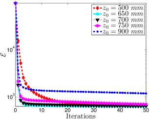
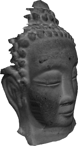
(a)	(b)	(c)

Figure 13: (a) Evolution of the energy $\mathcal{E}$ of the proposed approach, defined in (4.5), using least-squares estimation, in function of the iterations, for the data of Fig. 2. As long as the initial scale is not over-estimated too much, the proposed scheme converges towards similar solutions for different initial estimates (cf. Fig. 14), though with different speeds. (b) 3D-model obtained at convergence, using $z_{0}=750~{}mm$. (c) Histogram of point-to-point distances between (b) and the ground truth (cf. Fig. 7-c). As in the experiment of Fig. 12, the median value is $1.2~{}mm$, yet this result is almost independent from the initialization, and is obtained using a provably convergent algorithm.

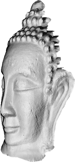
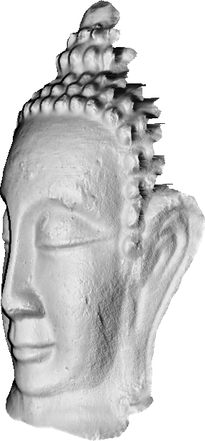
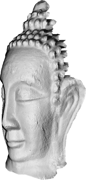
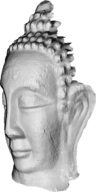
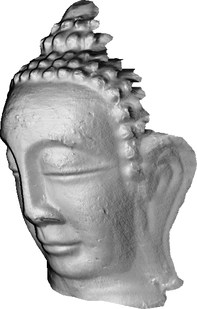
(a) $z_{0}=500~{}mm$	(b) $z_{0}=650~{}mm$	(c) $z_{0}=700~{}mm$	(d) $z_{0}=750~{}mm$	(e) $z_{0}=900~{}mm$

Figure 14: 3D-reconstructions after 50 iterations of the proposed scheme, taking as initial guess different fronto-parallel planes $z\equiv z_{0}$ and using least-squares estimation. Similar results are obtained whatever the initialization, at least as long as the initial scale is not over-estimated too much.

Although the accuracy of the results obtained with this new scheme is not improved, the influence of the initialization is much reduced and convergence is guaranteed. Besides, it is straightforward to improve robustness by simply changing the definitions of the function $\phi$ and of the operator $\{\cdotp\}_{+}$, while ensuring robustness of the ratio-based approach is not an easy task Mecca2016 ; Smith2016 . Fig. 15 shows the result obtained using Cauchy’s M-estimator $\Phi_{\text{Cauchy}}$ and explicit self-shadows handling i.e., $\{x\}_{+}=\max\{x,0\}$.

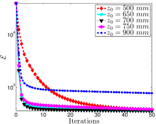
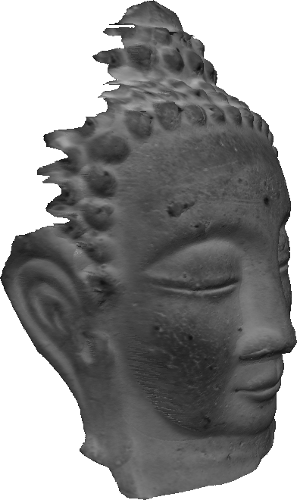
(a)	(b)	(c)

Figure 15: Same as Fig. 13, but using Cauchy’s robust M-estimator and explicit self-shadows handling. Despite the non-convexity of the estimator, convergence is similar to that obtained in the previous experiment. However, the median value of the 3D-reconstruction error is now $0.91~{}mm$, which is to be compared with the previous value $1.2~{}mm$ (cf. Fig. 13).

5 Estimating Colored 3D-models by Photometric Stereo

So far, we have considered only gray level images. In this section, we extend our study to RGB-valued images, in order to estimate colored 3D-models using photometric stereo. Similar to Section 2, we will first establish the image formation model and discuss calibration. Then, we will show how to modify the algorithm from Section 4 in order to handle RGB images.

5.1 Spectral Dependency of the Luminous Flux Emitted by a LED

We need to introduce a spectral dependency in Model (2.7) to extend our study to color. It seems reasonable to limit this dependency to the intensity ($\lambda$ denotes the wavelength):

$$\mathbf{s}(\mathbf{x},\lambda)=\Phi(\lambda)\,\cos^{\mu}\theta\,\frac{\mathbf{x}_{s}-\mathbf{x}}{\|\mathbf{x}_{s}-\mathbf{x}\|^{3}}.$$ (5.1)

Model (5.1) is more complex than Model (2.7), because the intensity $\Phi_{0}\in\mathbb{R}^{+}$ has been replaced by the emission spectrum $\Phi(\lambda)$, which is a function (cf. Fig. 16-a). The calibration of $\Phi(\lambda)$ could be achieved by using a spectrometer, but we will show how to extend the procedure from Section 2.2, which requires nothing else than a camera and two calibration patterns.

​​​​​	​​​​​​
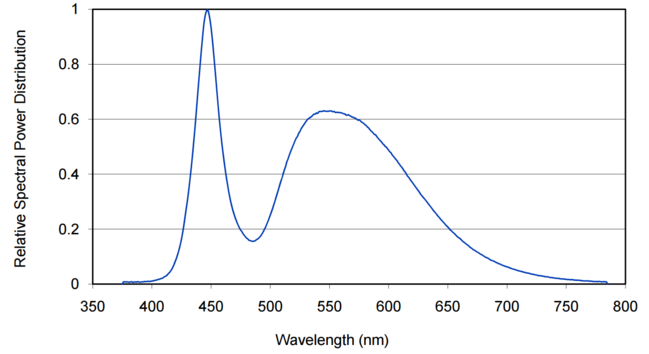
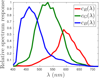
(a)	(b)

Figure 16: (a) Emission spectrum $\Phi(\lambda)$ of the LEDs used (source: http://www.lumileds.com/uploads/28/DS64-pdf). (b) Camera response functions in the three channels $R$, $G$, $B$, for the Canon EOS 50D camera Jiang2013 (which is similar to the Canon EOS 7D we use). Our extension to RGB images of the calibration procedure from Section 2.2 requires nothing else than a camera and two calibration patterns. Therefore, we do not need any of these diagrams in practice.

Given a point $\mathbf{x}$ of a Lambertian surface with albedo $\rho(\mathbf{x})$, under the illumination described by the lighting vector $\mathbf{s}(\mathbf{x})$, we get from (2.8), (2.9) and (2.10) the expression of the illuminance $\epsilon(\mathbf{p})$ of the image plane in the pixel $\mathbf{p}$ conjugate to $\mathbf{x}$:

$$\epsilon(\mathbf{p})=\beta\,\cos^{4}\alpha(\mathbf{p})\,\frac{\rho(\mathbf{x})}{\pi}\,\left\{\mathbf{s}(\mathbf{x})\cdot\mathbf{n}(\mathbf{x})\right\}_{+}.$$ (5.2)

This expression is easily extended to the case where $\mathbf{s}(\mathbf{x})$ and $\rho(\mathbf{x})$ depend on $\lambda$:

$$\epsilon(\mathbf{p},\lambda)=\beta\,\cos^{4}\alpha(\mathbf{p})\,\frac{\rho(\mathbf{x},\lambda)}{\pi}\,\left\{\mathbf{s}(\mathbf{x},\lambda)\cdot\mathbf{n}(\mathbf{x})\right\}_{+}.$$ (5.3)

The one-to-one correspondence between the points $\mathbf{x}$ and the pixels $\mathbf{p}$ allows us to denote $\rho(\mathbf{p},\lambda)$ and $\mathbf{n}(\mathbf{p})$, in lieu of $\rho(\mathbf{x},\lambda)$ and $\mathbf{n}(\mathbf{x})$. In addition, the light effectively received by each cell goes through a colored filter characterized by its transmission spectrum $c_{\star}(\lambda)$, $\star\in\{R,G,B\}$, whose maximum lies, respectively, in the red, green and blue ranges (cf. Fig. 16-b). To define the color levels $I_{\star}(\mathbf{p})$, $\star\in\{R,G,B\}$, by similarity with the expression (2.12) of the (corrected) gray level $I(\mathbf{p})$, we must multiply (5.3) by $c_{\star}(\lambda)$, and integrate over the entire spectrum:

$$I_{\star}(\mathbf{p})\!=\!\frac{\gamma\,\beta}{\pi}\,\left\{\left[\int_{\lambda=0}^{+\infty}\!\!c_{\star}(\lambda)\,\rho(\mathbf{p},\lambda)\,\mathbf{s}(\mathbf{x},\lambda)\,\mathrm{d}\lambda\right]\cdot\mathbf{n}(\mathbf{p})\right\}_{+}.$$ (5.4)

Using a Lambertian calibration pattern which is uniformly white i.e., such that $\rho(\mathbf{p},\lambda)\equiv\rho_{0}$, allows us to rewrite (5.4) as follows:

$$I_{\star}(\mathbf{p})=\gamma\,\beta\,\frac{\rho_{0}}{\pi}\,\left\{\left[\int_{\lambda=0}^{+\infty}\!\!\!\!\!\!\!c_{\star}(\lambda)\,\mathbf{s}(\mathbf{x},\lambda)\,\mathrm{d}\lambda\right]\cdot\mathbf{n}(\mathbf{p})\right\}_{+},$$ (5.5)

which is indeed an extension of (2.17) to RGB images, since (5.5) can be rewritten

$$I_{\star}(\mathbf{p})=\gamma\,\beta\,\frac{\rho_{0}}{\pi}\,\left\{\mathbf{s}_{\star}(\mathbf{x})\cdot\mathbf{n}(\mathbf{p})\right\}_{+},$$ (5.6)

provided that the three colored lighting vectors $\mathbf{s}_{\star}(\mathbf{x})$ are defined as follows:

$$\mathbf{s}_{\star}(\mathbf{x})=\int_{\lambda=0}^{+\infty}c_{\star}(\lambda)\,\mathbf{s}(\mathbf{x},\lambda)\,\mathrm{d}\lambda,\quad\star\in\{R,G,B\}.$$ (5.7)

Replacing the lighting vector $\mathbf{s}(\mathbf{x},\lambda)$ in (5.7) by its expression (5.1), we obtain the following extension of Model (2.7) to color:

$$\mathbf{s}_{\star}(\mathbf{x})=\Phi_{\star}\,\cos^{\mu}\theta\,\frac{\mathbf{x}_{s}-\mathbf{x}}{\|\mathbf{x}_{s}-\mathbf{x}\|^{3}},\qquad\star\in\{R,G,B\},$$ (5.8)

where the colored intensities $\Phi_{\star}$ are defined as follows:

$$\Phi_{\star}=\int_{\lambda=0}^{+\infty}c_{\star}(\lambda)\,\Phi(\lambda)\,\mathrm{d}\lambda,\qquad\star\in\{R,G,B\}.$$ (5.9)

The spectral dependency of the lighting vector $\mathbf{s}(\mathbf{x},\lambda)$ expressed in (5.1) is thus partially described by Model (5.8), which contains nine parameters: three for the coordinates of $\mathbf{x}_{s}$, two for the unit-length vector $\mathbf{n}_{s}$, plus the three colored intensities $\Phi_{R}$, $\Phi_{G}$, $\Phi_{B}$, and the anisotropy parameter $\mu$. Nonetheless, since the definition (5.9) of $\Phi_{\star}$ depends on $c_{\star}(\lambda)$, it follows that the parameters $\Phi_{R}$, $\Phi_{G}$ and $\Phi_{B}$ are not really characteristic of the LED, but of the camera-LED pair.

5.2 Spectral Calibration of the Luminous Flux Emitted by a LED

We use again the Lambertian planar calibration pattern from Section 2.2. Since it is convex, the incident light comes solely from the LED. We can thus replace $\mathbf{s}_{\star}(\mathbf{x})$ by its definition (5.8) in the expression (5.6) of the color level $I_{\star}(\mathbf{p})$. Assuming that $\mathbf{x}_{s}$ is estimated by triangulation and that the anisotropy parameter $\mu$ is provided by the manufacturer, we then have to solve, in each channel $\star\in\{R,G,B\}$, the following problem, which is an extension of Problem (2.19) ($q$ is the number of poses of the Lambertian calibration pattern):

$$\underset{\mathbf{m}_{s,\star}}{\operatorname{\min}~{}}\displaystyle\sum_{j=1}^{q}\!\sum_{\mathbf{p}\in\Omega^{j}}\!\!\left[\!\mathbf{m}_{s,\star}\!\cdot\!(\mathbf{x}^{j}\!-\!\mathbf{x}_{s})\!-\!\left[\!\displaystyle I_{\star}^{j}(\mathbf{p})\,\frac{\|\mathbf{x}_{s}\!-\!\mathbf{x}^{j}\|^{3+\mu}}{\left\{(\mathbf{x}_{s}\!-\!\mathbf{x}^{j})\cdot\mathbf{n}^{j}\right\}_{+}}\!\right]^{\!\frac{1}{\mu}}\right]^{\!2}\!\!,$$ (5.10)

where $\mathbf{m}_{s,\star}$ is defined by analogy with $\mathbf{m}_{s}$ (cf. (2.18)):

$$\mathbf{m}_{s,\star}={\Psi_{\star}}^{\frac{1}{\mu}}\,\mathbf{n}_{s},$$ (5.11)

and $\Psi_{\star}$ is defined by analogy with $\Psi$ (cf. (2.14)):

$$\Psi_{\star}=\gamma\,\beta\,\frac{\rho_{0}}{\pi}\,\Phi_{\star}.$$ (5.12)

Each problem (5.10) allows us to estimate a colored intensity $\Phi_{R}$, $\Phi_{G}$ or $\Phi_{B}$ (up to a common factor) and the principal direction $\mathbf{n}_{s}$, which is thus estimated three times. Table 1 groups the values obtained for one of the LEDs of our setup. The three estimates of $\mathbf{n}_{s}$ are consistent, but instead of arbitrarily choosing one of them, we compute the weighted mean of these estimates, using spherical coordinates.

Red channel	Green channel	Blue channel
$\widehat{\mathbf{n}}_{s,R}=\begin{bmatrix}0.205\\ -0.757\\ 0.621\end{bmatrix}$	$\widehat{\mathbf{n}}_{s,G}=\begin{bmatrix}0.194\\ -0.769\\ 0.608\end{bmatrix}$	$\widehat{\mathbf{n}}_{s,B}=\begin{bmatrix}0.188\\ -0.844\\ 0.503\end{bmatrix}$
$\widehat{\Psi}_{R}=3.10\times 10^{7}$	$\widehat{\Psi}_{G}=5.49\times 10^{7}$	$\widehat{\Psi}_{B}=3.37\times 10^{7}$

Table 1: Parameters of one of the LEDs of our setup, estimated by solving (5.10) in each color channel.

In Table 1, the values of $\widehat{\Psi}_{R}$, $\widehat{\Psi}_{G}$ and $\widehat{\Psi}_{B}$ are given without unit because, from the definition (5.12) of $\Psi_{\star}$, only their relative values are meaningful. As it happens, the value of $\widehat{\Psi}_{G}$ is roughly twice as much as those of $\widehat{\Psi}_{R}$ and $\widehat{\Psi}_{B}$, but this does not mean that $\Phi(\lambda)$ is twice higher in the green range than in the red or in the blue ranges, since the definition (5.9) of a given colored intensity $\Phi_{\star}$ also depends on the transmission spectrum $c_{\star}(\lambda)$ in the considered channel.

Our calibration procedure relies on the assumption that the calibration pattern is uniformly white i.e., that $\rho(\mathbf{p},\lambda)\equiv\rho_{0}$, which may be inexact, yet in no way does this question our rationale. Indeed, if we assume that the color of “white” cells from the Lambertian checkerboard (cf. Fig. 4) is uniform i.e., $\rho(\mathbf{p},\lambda)=\rho(\lambda)$, $\forall\mathbf{p}\in\Omega^{j}$, and if we denote $\rho_{0}$ the maximum value of $\rho(\lambda)$, Eq. (5.5) is still valid, provided that $c_{\star}(\lambda)$ is replaced by the function $\overline{c}_{\star}(\lambda)$ defined as follows:

$$\overline{c}_{\star}(\lambda)=\frac{\rho(\lambda)}{\rho_{0}}\,c_{\star}(\lambda).$$ (5.13)

5.3 Photometric Stereo under Colored Point Light Source Illumination

If we pretend to extend Model (2.21) to RGB images, then it must be possible to write the color level at $\mathbf{p}$, in each channel $\star\in\{R,G,B\}$, in the following manner:

$$\!I_{\star}(\mathbf{p})\!=\!\Psi_{\star}\,\frac{\rho_{\star}(\mathbf{p})}{\rho_{0}}\!\left[\!\frac{\mathbf{n}_{s}\!\cdot\!\left(\!\mathbf{x}\!-\!\mathbf{x}_{s}\!\right)}{\|\mathbf{x}\!-\!\mathbf{x}_{s}\|}\!\right]^{\mu}\frac{\left\{(\mathbf{x}_{s}\!-\!\mathbf{x})\!\cdot\!\mathbf{n}(\mathbf{p})\right\}_{+}}{\|\mathbf{x}_{s}\!-\!\mathbf{x}\|^{3}}$$ (5.14)

where the colored albedos $\rho_{\star}(\mathbf{p})$ are some extensions of the albedo $\rho(p)$ to the RGB case. Equating both expressions of $I_{\star}(\mathbf{p})$ given in (5.4) and in (5.14), and using the definition (5.1) of $\mathbf{s}(\mathbf{x},\lambda)$, we obtain:

$$\Psi_{\star}\frac{\rho_{\star}(\mathbf{p})}{\rho_{0}}\,=\frac{\gamma\beta}{\pi}\displaystyle\int_{\lambda=0}^{+\infty}\!\!\!c_{\star}(\lambda)\,\rho(\mathbf{p},\lambda)\,\Phi(\lambda)\,\mathrm{d}\lambda.$$ (5.15)

Using the definitions (5.12) and (5.9) of $\Psi_{\star}$ and $\Phi_{\star}$, (5.15) yields the following expression for the colored albedos:

$$\rho_{\star}(\mathbf{p})\!=\!\frac{\displaystyle\int_{\lambda=0}^{+\infty}\!\!\!c_{\star}(\lambda)\,\rho(\mathbf{p},\!\lambda)\,{\Phi}(\lambda)\,\mathrm{d}\lambda}{\displaystyle\int_{\lambda=0}^{+\infty}c_{\star}(\lambda)\,{\Phi}(\lambda)\,\mathrm{d}\lambda},\,\star\!\in\!\{\!R,\!G,\!B\},$$ (5.16)

which is the mean of $\rho(\mathbf{p},\lambda)$ over the entire spectrum, weighted by the product $c_{\star}(\lambda)\,{\Phi}(\lambda)$. In addition, although the transmission spectrum $c_{\star}(\lambda)$ depends only on the camera, the emission spectrum ${\Phi}(\lambda)$ usually varies from one LED to another. Thus, generalizing photometric stereo under point light source illumination to RGB images requires to superscript the colored albedos by the LED index $i$. Hence, it seems that we have to solve, in each pixel $\mathbf{p}\in\Omega$, the following problem:

$$I_{\star}^{i}(\mathbf{p})=\Psi^{i}_{\star}\,\frac{\rho^{i}_{\star}(\mathbf{p})}{\rho_{0}}\!\left[\!\frac{\mathbf{n}^{i}_{s}\!\cdot\!\left(\!\mathbf{x}\!-\!\mathbf{x}_{s}^{i}\!\right)}{\|\mathbf{x}\!-\!\mathbf{x}_{s}^{i}\|}\!\right]^{\mu^{i}}\frac{\left\{(\mathbf{x}_{s}^{i}\!-\!\mathbf{x})\!\cdot\!\mathbf{n}(\mathbf{p})\right\}_{+}}{\|\mathbf{x}_{s}^{i}\!-\!\mathbf{x}\|^{3}},$$

$$\qquad\qquad\qquad\quad~{}i\in\{1,\dots,m\},~{}\star\in\{R,G,B\}.$$ (5.17)

System (5.17) is underdetermined, because it contains $3m$ equations with $3m+3$ unknowns: one colored albedo $\rho_{\star}^{i}(\mathbf{p})$ per equation, the depth $z(\mathbf{p})$ of the 3D-point $\mathbf{x}$ conjugate to $\mathbf{p}$ (from which we get the coordinates of $\mathbf{x}$), and the normal $\mathbf{n}(\mathbf{p})$. Apart from this numerical difficulty, the dependency on $i$ of the colored albedos is puzzling: while it is clear that the albedo is a photometric characteristic of the surface, independent from the lighting, it should go the same for the colored albedos. This shows that the extension to RGB images of photometric stereo is potentially intractable in the general case. However, such an extension is known to be possible in two specific cases CVPR2016 :

• For a non-colored surface i.e., when $\rho(\mathbf{p},\lambda)=\rho(\mathbf{p})$, we deduce from (5.16) that $\rho_{R}(\mathbf{p})=\rho_{G}(\mathbf{p})=\rho_{B}(\mathbf{p})=\rho(\mathbf{p})$. Problem (5.17) is thus written:

  $$I_{\star}^{i}(\mathbf{p})=\Psi^{i}_{\star}\,\frac{\rho(\mathbf{p})}{\rho_{0}}\!\left[\!\frac{\mathbf{n}^{i}_{s}\!\cdot\!\left(\!\mathbf{x}\!-\!\mathbf{x}_{s}^{i}\!\right)}{\|\mathbf{x}\!-\!\mathbf{x}_{s}^{i}\|}\!\right]^{\mu^{i}}\frac{\left\{(\mathbf{x}_{s}^{i}\!-\!\mathbf{x})\!\cdot\!\mathbf{n}(\mathbf{p})\right\}_{+}}{\|\mathbf{x}_{s}^{i}\!-\!\mathbf{x}\|^{3}},$$

  $$\qquad\qquad\qquad i\in\{1,\dots,m\},~{}\star\in\{R,G,B\}.$$ (5.18)

  If the albedo is known, and if a channel dependency is added to the sources parameters $\mathbf{x}^{i}_{s}$, $\mathbf{n}^{i}_{s}$ and $\mu^{i}$, then System (5.18) has 3 unknowns and $3m$ independent equations: a single RGB image may suffice to ensure that the problem is well-determined. This well-known case, which dates back to the 90’s Kontsevich1994 , has been applied to real-time 3D-reconstruction of a white painted deformable surface Hernandez2007 .

• When the sources are non-colored i.e., when ${\Phi}^{i}(\lambda)\equiv\Phi_{0}$, $\forall i\in\{1,\dots,m\}$, (5.16) gives:

  $$\rho_{\star}(\mathbf{p})\!=\!\frac{\displaystyle\int_{\lambda=0}^{+\infty}\!\!\!c_{\star}(\lambda)\,\rho(\mathbf{p},\!\lambda)\,\mathrm{d}\lambda}{\displaystyle\int_{\lambda=0}^{+\infty}c_{\star}(\lambda)\,\mathrm{d}\lambda},~{}\star\in\{R,G,B\}.$$ (5.19)

  Since this expression is independent from $i$, Problem (5.17) is rewritten:

  $$I_{\star}^{i}(\mathbf{p})=\Psi_{\star}\,\frac{\rho_{\star}(\mathbf{p})}{\rho_{0}}\!\left[\!\frac{\mathbf{n}^{i}_{s}\!\cdot\!\left(\!\mathbf{x}\!-\!\mathbf{x}_{s}^{i}\!\right)}{\|\mathbf{x}\!-\!\mathbf{x}_{s}^{i}\|}\!\right]^{\mu^{i}}\frac{\left\{(\mathbf{x}_{s}^{i}\!-\!\mathbf{x})\!\cdot\!\mathbf{n}(\mathbf{p})\right\}_{+}}{\|\mathbf{x}_{s}^{i}\!-\!\mathbf{x}\|^{3}},$$

  $$\qquad\qquad\qquad i\in\{1,\dots,m\},~{}\star\in\{R,G,B\}.$$ (5.20)

  In (5.20), the parameter $\Psi_{\star}$ is independent from $i$, but it really depends on the channel $\star$, although the sources are supposed to be non-colored, since in the definition (5.12) of $\Psi_{\star}$, the colored intensity $\Phi_{\star}$ is channel-dependent (cf. Eq. (5.9)). System (5.20), which has $3m$ equations and six unknowns, is overdetermined if $m\geqslant 3$. If $m=2$, it is well-determined but rank-deficient, since in each point, the $6$ lighting vectors are coplanar. Additional information (e.g., a boundary condition) is required Mecca2014b .
  

Another case where the colored albedos are independent from $i$ is when the $m$ LEDs all share the same emission spectrum, up to multiplicative coefficients ($\Phi^{i}(\lambda)=\kappa^{i}\,\Phi(\lambda),\,\forall i\in\{1,\dots,m\}$). Under such an assumption, the colored albedos $\rho_{\star}(\mathbf{p})$ do not have to be indexed by $i$, according to their definition (5.16). Note however that the parameters $\Psi_{\star}$ still have to be indexed by $i$, in this case. Using the notation

$$\overline{\rho}_{\star}(\mathbf{p})=\frac{\rho_{\star}(\mathbf{p})}{\rho_{0}},\quad\star\in\{R,G,B\},$$ (5.21)

we obtain the following result:  

Under the same hypotheses as in Eq. (2.1), if the $m$ light sources share the same emission spectrum, up to a multiplicative coefficient, then the $m$ RGB images can be modeled as follows:

$$\!\!\!I_{\star}^{i}(\mathbf{p})\!=\!\Psi_{\star}^{i}\,\overline{\rho}_{\star}(\mathbf{p})\!\left[\frac{\mathbf{n}^{i}_{s}\!\cdot\!\left(\mathbf{x}-\mathbf{x}^{i}_{s}\right)}{\|\mathbf{x}-\mathbf{x}^{i}_{s}\|}\right]^{\mu^{i}}\!\!\frac{\left\{(\mathbf{x}^{i}_{s}-\mathbf{x})\cdot\mathbf{n}(\mathbf{p})\right\}_{+}}{\|\mathbf{x}^{i}_{s}-\mathbf{x}\|^{3}},$$

$$\qquad\qquad\qquad\quad\,i\in\{1,\dots,m\},\,\star\in\{R,G,B\}.$$ (5.22)

where:

• $I^{i}_{\star}$ is the (corrected) color level in channel $\star$;

• $\Psi_{R}^{i}$, $\Psi_{G}^{i}$ and $\Psi_{B}^{i}$ are the colored intensities of the $i$-th source, multiplied by an unknown factor, which is common to all the sources and depends on several camera parameters and on the albedo $\rho_{0}$ (cf. Eqs. (5.9) and (5.12));

• $\overline{\rho}_{\star}$ is the colored albedo in channel $\star$, relatively to $\rho_{0}$ (cf. Eq. (5.21)).

For the setup of Fig. 2-a, the $m=8$ LEDs probably do not exactly share the same spectrum, although they come from the same batch, yet this assumption seems more realistic than that of “non-colored sources”, and it allows us to better justify the use of (5.22), which models both the spectral dependency of the albedo and that of the luminous fluxes.

The calibration procedure described in Section 5.2 provides us with the values of the parameters $\mathbf{x}^{i}_{s}$, $\mathbf{n}^{i}_{s}$ and $\Psi_{\star}^{i}$, $i\in\{1,\dots,m\}$, and the parameters $\mu^{i}$, $i\in\{1,\dots,m\}$, are provided by the manufacturer. The unknowns of System (5.22) are thus the depth $z(\mathbf{p})$ of $\mathbf{x}$, the normal $\mathbf{n}(\mathbf{p})$ and the three colored albedos $\overline{\rho}_{\star}(\mathbf{p})$, $\star\in\{R,G,B\}$. Resorting to RGB images allows us to replace the system (2.1) of $m$ equations with four unknowns, by the system (5.22) of $3m$ equations with six unknowns, which should yield more accurate results.

5.4 Solving Colored Photometric Stereo under Point Light Source Illumination

The alternating strategy from Section 3.1 is not straightforward to adapt to the case of RGB-valued images, because the albedo is channel-dependent, while the normal vector is not. Principal component analysis could be employed Barsky2003 , but we already know from Section 3 that a differential approach should be preferred anyway.

A PDE-based approach similar to that of Section 3.2 is advocated in CVPR2016 : ratios between color levels can be computed in each channel $\star\in\{R,G,B\}$, thus eliminating the colored albedos $\overline{\rho}_{\star}(\mathbf{p})$ and obtaining a system of PDEs in $z$ similar to (3.23). The PDEs to solve remain quasi-linear, unlike in Ikeda2008 . Yet, we know that the solution strongly depends on the initialization.

On the other hand, it is straightforward to adapt the method recommended in Section 4, by turning the discrete optimization problem (4.5) into

$$\min_{\begin{subarray}{c}\tilde{\bm{\rho}}_{R},\tilde{\bm{\rho}}_{G},\tilde{\bm{\rho}}_{B},\tilde{\bm{z}}\end{subarray}}\sum_{\star\in\{R,G,B\}}\sum_{j=1}^{n}\sum_{i=1}^{m}\phi\left(r^{i}_{\star,j}(\tilde{\bm{\rho}}_{\star},\tilde{\bm{z}})\right),$$ (5.23)

with the following new definitions, which use straightforward notations for the channel dependencies:

$$r^{i}_{\star,j}(\tilde{\bm{\rho}}_{\star},\tilde{\bm{z}})=\tilde{\rho}_{\star,j}\left\{\zeta^{i}_{\star,j}(\tilde{\bm{z}})\right\}_{+}-I^{i}_{\star,j},$$ (5.24)

$$\zeta^{i}_{\star,j}(\tilde{\bm{z}})=\left[\mathbf{Q}_{j}\mathbf{t}^{i}_{\star,j}(\tilde{z}_{j})\right]\cdot\begin{bmatrix}(\nabla\tilde{\bm{z}})_{j}\\ -1\end{bmatrix}.$$ (5.25)

The actual solution of (5.23) follows immediately from the algorithm described in Section 4.2. The depth update simply uses three times more equations, which improves its robustness, while the estimation of each colored albedo is carried out independently in each channel in exactly the same way as in Section 4.2.

Since the depth estimation now uses more data, the 3D-model of Fig. 17, which uses RGB images, is improved in two ways, in comparison with that of Fig. 15: it is not only colored, but also more accurate.

(a)

(b)

Figure 17: (a) 3D-model estimated from the $m=8$ images of Fig. 2, which are RGB images. (b) Histogram of the distances between this 3D-shape and the ground truth (cf. Fig. 7-c). Using RGB images improves the result, in comparison with the experiment of Fig. 15: the median of the point-to-point distances to the ground truth is now equal to $0.85~{}mm$.

6 Conclusion and Perspectives

In this article, we describe a photometric stereo-based 3D-reconstruction setup using LEDs as light sources. We first model the luminous flux emitted by a LED, then the resulting photometric stereo problem. We present a practical procedure for calibrating photometric stereo under point light source illumination, and eventually, we study several numerical solutions. Existing methods are based either on alternating estimation of normals and depth, or on direct depth estimation using image ratios. Both these methods have their own advantages, but their convergence is not established. Hence, we introduce a new, provably convergent solution based on alternating reweighted least-squares. Finally, we extend the whole study to RGB images.

The result of Fig. 18 suggests that our goal i.e., the estimation of colored 3D-models of faces by photometric stereo, has been reached. Of course, many other types of 3D-scanners exist, but ours relies only on materials which are easy to obtain: a relatively mainstream camera, eight LEDs and an Arduino controller to synchronize the LEDs with the shutter release. Another significant advantage of our 3D-scanner is that it also estimates the albedo.

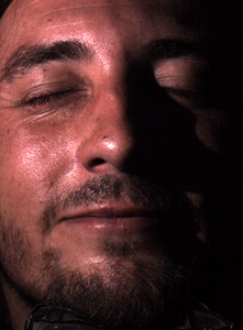
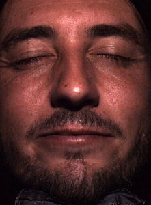
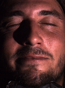
(a)	(b)	(c)

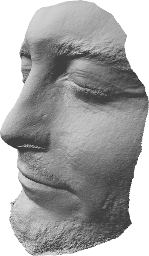
(d)	(e)

Figure 18: (a-b-c) Three RGB images (out of $m=8$) of a face captured by our setup. (d) Estimated 3D-shape. (e) Colored 3D-model. Since their estimation is relative to the Lambertian planar calibration pattern, the colored albedos of the 3D-model may appear different from the colors of the images.

However, there may still be some points where the shape, and therefore the albedo, are poorly estimated. In the example of Fig. 19, the area under the nose, which is dimly lit, is poorly reconstructed (this problem does not appear in the example of Fig. 18, because the face is oriented in such a way that it is “well” illuminated). Although such artifacts remain confined, thanks to robust estimation, future extensions of our work could get rid of them by resorting to an additional regularization term in the variational model.

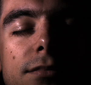
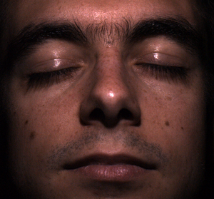
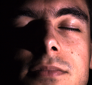
(a)	(b)	(c)

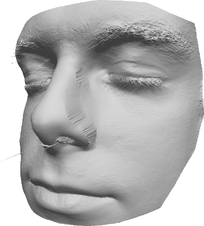
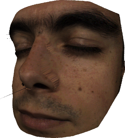
(d)	(e)

Figure 19: (a-b-c) Three images (out of $m=8$) of a face. (d) Estimated 3D-shape. (e) Colored 3D-model. The 3D-reconstruction is not satisfactory under the nose, which is a dimly lit area. Robustness of the proposed method to shadows could still be improved.

Besides dealing with these defects, other questions arise. In particular, could we extend our 3D-scanner to full 3D-reconstruction, by coupling the proposed method with multi-view 3D-reconstruction techniques Hernandez2008 ? Aside from obtaining a more complete 3D-reconstruction, this would circumvent the difficult problem of handling possible discontinuities in a depth map, although Fig. 19 suggests that employing a non-convex estimator already partly allows the recovery of such sharp structures Durou2009 .

Eventually, the proposed numerical framework could be extended in order to automatically refine calibration. Several steps in that direction were already achieved in Logothetis2017 ; Migita2008 ; Papadhimitri2014b ; SSVM2017 , but either without convergence analysis Logothetis2017 ; Migita2008 ; Papadhimitri2014b or in the restricted case where only the source intensities are refined SSVM2017 . Providing a provably convergent method for uncalibrated photometric stereo under point light source illumination would thus constitute a natural extension of our work.

Appendix A Proof of Lemma 1

Proof

First note that, under the condition (4.29), the function $\mathcal{E}(\cdot,\tilde{\bm{z}})$ (resp. $\tilde{\mathcal{E}}_{\tilde{\bm{z}}}(\cdot;\tilde{\bm{\rho}},\tilde{\bm{z}})$) is twice continuously differentiable at $\tilde{\bm{\rho}}$ (resp. $\tilde{\bm{z}}$), whenever $(\tilde{\bm{\rho}},\tilde{\bm{z}})$ is sufficiently close to $(\tilde{\bm{\rho}}^{*},\tilde{\bm{z}}^{*})$. The corresponding second-order derivatives are calculated as follows:

$$\delta\tilde{\bm{\rho}}^{\top}\frac{\partial^{2}\mathcal{E}}{\partial\tilde{\bm{\rho}}^{2}}(\tilde{\bm{\rho}},\tilde{\bm{z}})\delta\tilde{\bm{\rho}}=\sum_{j=1}^{n}\sum_{i=1}^{m}\phi^{\prime\prime}(r^{i}_{j}(\tilde{\bm{\rho}},\tilde{\bm{z}}))\left(\delta\tilde{\rho}_{j}\{\zeta^{i}_{j}(\tilde{\bm{z}})\}_{+}\right)^{2},$$ (A.1)

$$\delta\tilde{\bm{z}}^{\top}\partial^{2}\tilde{\mathcal{E}}_{\tilde{\bm{z}}}(\tilde{\bm{z}};\tilde{\bm{\rho}},\tilde{\bm{z}})\delta\tilde{\bm{z}}$$

$$\quad=\sum_{j=1}^{n}\sum_{i=1}^{m}\phi^{\prime\prime}(r^{i}_{j}(\tilde{\bm{\rho}},\tilde{\bm{z}}))\left(\tilde{\rho}_{j}\,\chi(\zeta^{i}_{j}(\tilde{\bm{z}}))\,\delta\tilde{\bm{z}}^{\top}\partial\zeta^{i}_{j}(\tilde{\bm{z}})\right)^{2}.$$ (A.2)

Comparing the above two formulas with (4.21) and (4.25), the conclusion follows from condition (4.8). ∎

Appendix B Proof of Theorem 4.1

Proof

First note that condition (4.32) implies that

$$\dfrac{\partial^{2}\mathcal{E}}{\partial\tilde{\bm{\rho}}^{2}}(\tilde{\bm{\rho}}^{*},\tilde{\bm{z}}^{*})\succ{\bm{O}},$$ (B.1)

$$\frac{\partial^{2}\mathcal{E}}{\partial\tilde{\bm{z}}^{2}}(\tilde{\bm{\rho}}^{*}\!,\tilde{\bm{z}}^{*})-\dfrac{\partial^{2}\mathcal{E}}{\partial\tilde{\bm{\rho}}\partial\tilde{\bm{z}}}(\tilde{\bm{\rho}}^{*}\!,\tilde{\bm{z}}^{*})\dfrac{\partial^{2}\mathcal{E}}{\partial\tilde{\bm{\rho}}^{2}}(\tilde{\bm{\rho}}^{*}\!,\tilde{\bm{z}}^{*})^{-1}\dfrac{\partial^{2}\mathcal{E}}{\partial\tilde{\bm{\rho}}\partial\tilde{\bm{z}}}(\tilde{\bm{\rho}}^{*}\!,\tilde{\bm{z}}^{*})\succ{\bm{O}}.$$ (B.2)

Utilizing Lemma 1 in conjunction with (B.2) and (4.33), we obtain

$$H_{\tilde{\bm{\rho}}}(\tilde{\bm{\rho}}^{*},\tilde{\bm{z}}^{*})\succ{\bm{O}},\qquad H_{\tilde{\bm{z}}}(\tilde{\bm{\rho}}^{*},\tilde{\bm{z}}^{*})\succ{\bm{O}},$$ (B.3)

$$\frac{\partial^{2}\mathcal{E}}{\partial\tilde{\bm{z}}^{2}}(\tilde{\bm{\rho}}^{*}\!,\!\tilde{\bm{z}}^{*}\!)-\dfrac{\partial^{2}\mathcal{E}}{\partial\tilde{\bm{\rho}}\partial\tilde{\bm{z}}}(\tilde{\bm{\rho}}^{*}\!,\!\tilde{\bm{z}}^{*}\!)H_{\tilde{\bm{\rho}}}(\tilde{\bm{\rho}}^{*},\tilde{\bm{z}}^{*})^{-1}\dfrac{\partial^{2}\mathcal{E}}{\partial\tilde{\bm{\rho}}\partial\tilde{\bm{z}}}(\tilde{\bm{\rho}}^{*}\!,\!\tilde{\bm{z}}^{*})\succ{\bm{O}}.$$ (B.4)

Now consider the iteration

$$\tilde{\bm{z}}^{(k+1)}=\tilde{\bm{z}}^{(k)}-H_{\tilde{\bm{z}}}\left(\tilde{\bm{\rho}}^{(k+1)},\tilde{\bm{z}}^{(k)}\right)^{-1}\frac{\partial\mathcal{E}}{\partial\tilde{\bm{z}}}(\tilde{\bm{\rho}}^{(k+1)},\tilde{\bm{z}}^{(k)})$$

$$=\tilde{\bm{z}}^{(k)}\!-\!H_{\tilde{\bm{z}}}\!\!\left(\!\tilde{\bm{\rho}}^{(k)}\!\!-\!H_{\tilde{\bm{\rho}}}(\!\tilde{\bm{\rho}}^{(k)}\!\!,\!\tilde{\bm{z}}^{(k)}\!)^{-1}\frac{\partial\mathcal{E}}{\partial\tilde{\bm{\rho}}}(\tilde{\bm{\rho}}^{(k)}\!\!,\!\tilde{\bm{z}}^{(k)}\!),\!\tilde{\bm{z}}^{(k)}\!\!\right)^{\!-1}$$

$$\qquad~{}\frac{\partial\mathcal{E}}{\partial\tilde{\bm{z}}}\!\left(\!\tilde{\bm{\rho}}^{(k)}\!-\!H_{\tilde{\bm{\rho}}}(\tilde{\bm{\rho}}^{(k)}\!,\tilde{\bm{z}}^{(k)})^{-1}\frac{\partial\mathcal{E}}{\partial\tilde{\bm{\rho}}}(\tilde{\bm{\rho}}^{(k)},\tilde{\bm{z}}^{(k)}),\tilde{\bm{z}}^{(k)}\!\right)$$ (B.5)

as a map $\tilde{\bm{z}}^{(k)}\mapsto\tilde{\bm{z}}^{(k+1)}$. By the Ostrowski theorem (Ortega1970, , Proposition 10.1.3), the local convergence of $\{\tilde{\bm{z}}^{(k)}\}$ to $\tilde{\bm{z}}^{*}$ follows if the spectral radius of the Jacobian

$$\frac{\partial\tilde{\bm{z}}^{(k+1)}}{\partial\tilde{\bm{z}}^{(k)}}(\tilde{\bm{\rho}}^{*},\tilde{\bm{z}}^{*}) =\text{id}-H_{\tilde{\bm{z}}}(\tilde{\bm{\rho}}^{*},\tilde{\bm{z}}^{*})^{-1}\frac{\partial^{2}\mathcal{E}}{\partial\tilde{\bm{z}}^{2}}(\tilde{\bm{\rho}}^{*},\tilde{\bm{z}}^{*})$$

$$\!\!\!\!\!\!\!\!\!\!\!\!\!\!\!\!\!\!\!\!\!\!\!\!\!\!\!\!\!\!\!\!\!\!\!\!\!\!\!\!\!\!+H_{\tilde{\bm{z}}}(\tilde{\bm{\rho}}^{*},\tilde{\bm{z}}^{*})^{-1}\frac{\partial^{2}\mathcal{E}}{\partial\tilde{\bm{\rho}}\partial\tilde{\bm{z}}}(\tilde{\bm{\rho}}^{*},\tilde{\bm{z}}^{*})H_{\tilde{\bm{\rho}}}(\tilde{\bm{\rho}}^{*},\tilde{\bm{z}}^{*})^{-1}$$

$$\!\!\!\!\!\!\!\!\!\!\!\!\!\!\!\!\!\!\!\!\!\!\!\!\!\!\!\!\!\!\!\!\!\!\!\frac{\partial^{2}\mathcal{E}}{\partial\tilde{\bm{\rho}}\partial\tilde{\bm{z}}}(\tilde{\bm{\rho}}^{*},\tilde{\bm{z}}^{*})$$ (B.6)

is strictly less than 1. Using the similarity transform with $H_{\tilde{\bm{z}}}(\tilde{\bm{\rho}}^{*},\tilde{\bm{z}}^{*})^{\frac{1}{2}}$, we derive:

$$\mathrm{sr}\left(\frac{\partial\tilde{\bm{z}}^{(k+1)}}{\partial\tilde{\bm{z}}^{k}}(\tilde{\bm{\rho}}^{*},\tilde{\bm{z}}^{*})\right)$$

$$\quad=\mathrm{sr}\left(H_{\tilde{\bm{z}}}(\tilde{\bm{\rho}}^{*},\tilde{\bm{z}}^{*})^{\frac{1}{2}}\frac{\partial\tilde{\bm{z}}^{(k+1)}}{\partial\tilde{\bm{z}}^{k}}(\tilde{\bm{\rho}}^{*},\tilde{\bm{z}}^{*})H_{\tilde{\bm{z}}}(\tilde{\bm{\rho}}^{*},\tilde{\bm{z}}^{*})^{-\frac{1}{2}}\right)$$ (B.7)

$$\quad=\mathrm{sr}\bigg{(}\text{id}-H_{\tilde{\bm{z}}}(\tilde{\bm{\rho}}^{*},\tilde{\bm{z}}^{*})^{-\frac{1}{2}}\frac{\partial^{2}\mathcal{E}}{\partial\tilde{\bm{z}}^{2}}(\tilde{\bm{\rho}}^{*},\tilde{\bm{z}}^{*})H_{\tilde{\bm{z}}}(\tilde{\bm{\rho}}^{*},\tilde{\bm{z}}^{*})^{-\frac{1}{2}}$$

$$\qquad\quad+H_{\tilde{\bm{z}}}(\tilde{\bm{\rho}}^{*},\tilde{\bm{z}}^{*})^{-\frac{1}{2}}\frac{\partial^{2}\mathcal{E}}{\partial\tilde{\bm{\rho}}\partial\tilde{\bm{z}}}(\tilde{\bm{\rho}}^{*},\tilde{\bm{z}}^{*})H_{\tilde{\bm{\rho}}}(\tilde{\bm{\rho}}^{*},\tilde{\bm{z}}^{*})^{-1}$$

$$\qquad\qquad\qquad\qquad\quad\frac{\partial^{2}\mathcal{E}}{\partial\tilde{\bm{\rho}}\partial\tilde{\bm{z}}}(\tilde{\bm{\rho}}^{*},\tilde{\bm{z}}^{*})H_{\tilde{\bm{z}}}(\tilde{\bm{\rho}}^{*},\tilde{\bm{z}}^{*})^{-\frac{1}{2}}\bigg{)}$$ (B.8)

$$\quad=\sup_{\|\mathbf{v}\|=1}\bigg{|}\|\mathbf{v}\|^{2}$$

$$\qquad-\mathbf{v}^{\top}H_{\tilde{\bm{z}}}(\tilde{\bm{\rho}}^{*},\tilde{\bm{z}}^{*})^{-\frac{1}{2}}\frac{\partial^{2}\mathcal{E}}{\partial\tilde{\bm{z}}^{2}}(\tilde{\bm{\rho}}^{*},\tilde{\bm{z}}^{*})H_{\tilde{\bm{z}}}(\tilde{\bm{\rho}}^{*},\tilde{\bm{z}}^{*})^{-\frac{1}{2}}\mathbf{v}$$

$$\qquad+\mathbf{v}^{\top}H_{\tilde{\bm{z}}}(\tilde{\bm{\rho}}^{*},\tilde{\bm{z}}^{*})^{-\frac{1}{2}}\frac{\partial^{2}\mathcal{E}}{\partial\tilde{\bm{\rho}}\partial\tilde{\bm{z}}}(\tilde{\bm{\rho}}^{*},\tilde{\bm{z}}^{*})H_{\tilde{\bm{\rho}}}(\tilde{\bm{\rho}}^{*},\tilde{\bm{z}}^{*})^{-1}$$

$$\qquad\qquad\qquad\qquad\frac{\partial^{2}\mathcal{E}}{\partial\tilde{\bm{\rho}}\partial\tilde{\bm{z}}}(\tilde{\bm{\rho}}^{*},\tilde{\bm{z}}^{*})H_{\tilde{\bm{z}}}(\tilde{\bm{\rho}}^{*},\tilde{\bm{z}}^{*})^{-\frac{1}{2}}\mathbf{v}\bigg{|}.$$ (B.9)

It follows from condition (4.34) that

$$\frac{\partial^{2}\mathcal{E}}{\partial\tilde{\bm{z}}^{2}}(\tilde{\bm{\rho}}^{*},\tilde{\bm{z}}^{*})\prec 2\partial^{2}\tilde{\mathcal{E}}_{\tilde{\bm{z}}}(\tilde{\bm{z}}^{*};\tilde{\bm{\rho}}^{*},\tilde{\bm{z}}^{*})\preceq 2H_{\tilde{\bm{z}}}(\tilde{\bm{\rho}}^{*},\tilde{\bm{z}}^{*}),$$ (B.10)

and hence

$$\text{id}-H_{\tilde{\bm{z}}}(\tilde{\bm{\rho}}^{*},\tilde{\bm{z}}^{*})^{-\frac{1}{2}}\frac{\partial^{2}\mathcal{E}}{\partial\tilde{\bm{z}}^{2}}(\tilde{\bm{\rho}}^{*},\tilde{\bm{z}}^{*})H_{\tilde{\bm{z}}}(\tilde{\bm{\rho}}^{*},\tilde{\bm{z}}^{*})^{-\frac{1}{2}}\succ-\text{id}.$$ (B.11)

Consequently, there exists $\epsilon_{1}\in(0,1)$ such that the following inequality holds for an arbitrary $\mathbf{v}$:

$$\|\mathbf{v}\|^{2}-\mathbf{v}^{\top}H_{\tilde{\bm{z}}}(\tilde{\bm{\rho}}^{*},\tilde{\bm{z}}^{*})^{-\frac{1}{2}}\frac{\partial^{2}\mathcal{E}}{\partial\tilde{\bm{z}}^{2}}(\tilde{\bm{\rho}}^{*},\tilde{\bm{z}}^{*})H_{\tilde{\bm{z}}}(\tilde{\bm{\rho}}^{*},\tilde{\bm{z}}^{*})^{-\frac{1}{2}}\mathbf{v}$$

$$\qquad\qquad\qquad\qquad\qquad\qquad\qquad\quad\geq-(1-\epsilon_{1})\|\mathbf{v}\|^{2}.$$ (B.12)

Meanwhile, condition (B.4) implies that, for some $\epsilon_{2}\in(0,1)$:

$$\mathbf{v}^{\top}H_{\tilde{\bm{z}}}(\tilde{\bm{\rho}}^{*},\tilde{\bm{z}}^{*})^{-\frac{1}{2}}\frac{\partial^{2}\mathcal{E}}{\partial\tilde{\bm{z}}^{2}}(\tilde{\bm{\rho}}^{*},\tilde{\bm{z}}^{*})H_{\tilde{\bm{z}}}(\tilde{\bm{\rho}}^{*},\tilde{\bm{z}}^{*})^{-\frac{1}{2}}\mathbf{v}$$

$$\qquad-\mathbf{v}^{\top}H_{\tilde{\bm{z}}}(\tilde{\bm{\rho}}^{*},\tilde{\bm{z}}^{*})^{-\frac{1}{2}}\frac{\partial^{2}\mathcal{E}}{\partial\tilde{\bm{\rho}}\partial\tilde{\bm{z}}}(\tilde{\bm{\rho}}^{*},\tilde{\bm{z}}^{*})H_{\tilde{\bm{\rho}}}(\tilde{\bm{\rho}}^{*},\tilde{\bm{z}}^{*})^{-1}$$

$$\qquad\qquad\qquad\qquad\frac{\partial^{2}\mathcal{E}}{\partial\tilde{\bm{\rho}}\partial\tilde{\bm{z}}}(\tilde{\bm{\rho}}^{*},\tilde{\bm{z}}^{*})H_{\tilde{\bm{z}}}(\tilde{\bm{\rho}}^{*},\tilde{\bm{z}}^{*})^{-\frac{1}{2}}\mathbf{v}$$

$$=(H_{\tilde{\bm{z}}}(\tilde{\bm{\rho}}^{*},\tilde{\bm{z}}^{*})^{-\frac{1}{2}}\mathbf{v})^{\top}$$

$$\quad\Big{(}\frac{\partial^{2}\mathcal{E}}{\partial\tilde{\bm{z}}^{2}}(\tilde{\bm{\rho}}^{*},\tilde{\bm{z}}^{*})-\frac{\partial^{2}\mathcal{E}}{\partial\tilde{\bm{\rho}}\partial\tilde{\bm{z}}}(\tilde{\bm{\rho}}^{*},\tilde{\bm{z}}^{*})H_{\tilde{\bm{\rho}}}(\tilde{\bm{\rho}}^{*},\tilde{\bm{z}}^{*})^{-1}\frac{\partial^{2}\mathcal{E}}{\partial\tilde{\bm{\rho}}\partial\tilde{\bm{z}}}(\tilde{\bm{\rho}}^{*},\tilde{\bm{z}}^{*})\Big{)}$$

$$\quad\left(H_{\tilde{\bm{z}}}(\tilde{\bm{\rho}}^{*},\tilde{\bm{z}}^{*})^{-\frac{1}{2}}\mathbf{v}\right)$$ (B.13)

$$\geq\epsilon_{2}\|\mathbf{v}\|^{2}.$$ (B.14)

Altogether, we conclude

$$\mathrm{sr}\left(\frac{\partial\tilde{\bm{z}}^{(k+1)}}{\partial\tilde{\bm{z}}^{k}}(\tilde{\bm{\rho}}^{*},\tilde{\bm{z}}^{*})\right)\leq 1-\min(\epsilon_{1},\epsilon_{2}),$$ (B.15)

and hence the convergence of $\{\tilde{\bm{z}}^{(k)}\}$. The convergence of $\{\tilde{\bm{\rho}}^{(k)}\}$ to $\tilde{\bm{\rho}}^{*}$ follows from a similar argument. ∎

References

- (1) Ackermann, J., Fuhrmann, S., Goesele, M.: Geometric Point Light Source Calibration. In: Proceedings of the 18th International Workshop on Vision, Modeling & Visualization, pp. 161–168. Lugano, Switzerland (2013)
- (2) Ahmad, J., Sun, J., Smith, L., Smith, M.: An improved photometric stereo through distance estimation and light vector optimization from diffused maxima region. Pattern Recognition Letters 50, 15–22 (2014)
- (3) Angelopoulou, M.E., Petrou, M.: Uncalibrated flatfielding and illumination vector estimation for photometric stereo face reconstruction. Machine Vision and Applications 25(5), 1317–1332 (2013)
- (4) Aoto, T., Taketomi, T., Sato, T., Mukaigawa, Y., Yokoya, N.: Position estimation of near point light sources using a clear hollow sphere. In: Proceedings of the 21st International Conference on Pattern Recognition, pp. 3721–3724. Tsukuba, Japan (2012)
- (5) Barsky, S., Petrou, M.: The 4-source photometric stereo technique for three-dimensional surfaces in the presence of highlights and shadows. IEEE Transactions on Pattern Analysis and Machine Intelligence 25(10), 1239–1252 (2003)
- (6) Basri, R., Jacobs, D.W.: Lambertian reflectance and linear subspaces. IEEE Transactions on Pattern Analysis and Machine Intelligence 25(2), 218–233 (2003)
- (7) Bennahmias, M., Arik, E., Yu, K., Voloshenko, D., Chua, K., Pradhan, R., Forrester, T., Jannson, T.: Modeling of non-Lambertian sources in lighting applications. In: Optical Engineering and Applications, Proceedings of SPIE, vol. 6669. San Diego, USA (2007)
- (8) Bony, A., Bringier, B., Khoudeir, M.: Tridimensional reconstruction by photometric stereo with near spot light sources. In: Proceedings of the 21st European Signal Processing Conference. Marrakech, Morocco (2013)
- (9) Boyd, S., Parikh, N., Chu, E., Peleato, B., Eckstein, J.: Distributed Optimization and Statistical Learning via the Alternating Direction Method of Multipliers. Foundations and Trends in Machine Learning 3(1), 1–122 (2011)
- (10) Bringier, B., Bony, A., Khoudeir, M.: Specularity and shadow detection for the multisource photometric reconstruction of a textured surface. Journal of the Optical Society of America A 29(1), 11–21 (2012)
- (11) Ciortan, I., Pintus, R., Marchioro, G., Daffara, C., Giachetti, A., Gobbetti, E.: A Practical Reflectance Transformation Imaging Pipeline for Surface Characterization in Cultural Heritage. In: Proceedings of the 14th Eurographics Workshop on Graphics and Cultural Heritage. Genova, Italy (2016)
- (12) Clark, J.J.: Active photometric stereo. In: Proceedings of the IEEE Conference on Computer Vision and Pattern Recognition, pp. 29–34 (1992)
- (13) Collins, T., Bartoli, A.: 3D Reconstruction in Laparoscopy with Close-Range Photometric Stereo. In: Proceedings of the 15th International Conference on Medical Imaging and Computer Assisted Intervention, pp. 634–642. Nice, France (2012)
- (14) Durou, J.D., Aujol, J.F., Courteille, F.: Integrating the Normal Field of a Surface in the Presence of Discontinuities. In: Proceedings of the 7th International Conference on Energy Minimization Methods in Computer Vision and Pattern Recognition, Lecture Notes in Computer Science, vol. 5681, pp. 261–273. Bonn, Germany (2009)
- (15) Gabay, D., Mercier, B.: A dual algorithm for the solution of nonlinear variational problems via finite element approximation. Computers & Mathematics with Applications 2(1), 17–40 (1976)
- (16) Gardner, I.C.: Validity of the cosine-fourth-power law of illumination. Journal of Research of the National Bureau of Standards 39, 213–219 (1947)
- (17) Giachetti, A., Daffara, C., Reghelin C. Gobbetti, E., Pintus, R.: Light calibration and quality assessment methods for reflectance transformation imaging applied to artworks’ analysis. In: Optics for Arts, Architecture, and Archaeology V, Proceedings of SPIE, vol. 9527. Munich, Germany (2015)
- (18) Glowinski, R., Marroco, A.: Sur l’approximation, par éléments finis d’ordre un, et la résolution, par pénalisation-dualité d’une classe de problèmes de Dirichlet non linéaires. ESAIM: Mathematical Modelling and Numerical Analysis - Modélisation Mathématique et Analyse Numérique 9(2), 41–76 (1975)
- (19) Golub, G.H., Van Loan, C.F.: Matrix computations, 4 edn. The John Hopkings University Press (2013)
- (20) Gotardo, P.F.U., Simon, T., Sheikh, Y., Matthews, I.: Photogeometric Scene Flow for High-Detail Dynamic 3D Reconstruction. In: Proceedings of the IEEE International Conference on Computer Vision, pp. 846–854. Santiago, Chile (2015)
- (21) Gratton, S., Lawless, S., Nichols, N.K.: Approximate Gauss-Newton methods for nonlinear least squares problems. SIAM Journal on Optimization 18, 106–132 (2007)
- (22) Hara, K., Nishino, K., Ikeuchi, K.: Light source position and reflectance estimation from a single view without the distant illumination assumption. IEEE Transactions on Pattern Analysis and Machine Intelligence 27(4), 493–505 (2005)
- (23) Hernández, C., Vogiatzis, G., Brostow, G.J., Stenger, B., Cipolla, R.: Non-rigid Photometric Stereo with Colored Lights. In: Proceedings of the 11th IEEE International Conference on Computer Vision. Rio de Janeiro, Brazil (2007)
- (24) Hernández, C., Vogiatzis, G., Cipolla, R.: Multiview Photometric Stereo. IEEE Transactions on Pattern Analysis and Machine Intelligence 30(3), 548–554 (2008)
- (25) Hinkley, D.V.: On the Ratio of Two Correlated Normal Random Variables. Biometrika 56(3), 635–639 (1969)
- (26) Hoeltgen, L., Quéau, Y., Breuss, M., Radow, G.: Optimised photometric stereo via non-convex variational minimisation. In: Proceedings of the 27th British Machine Vision Conference. York, UK (2016)
- (27) Horn, B.K.P.: Robot Vision. The MIT Press (1986)
- (28) Horn, B.K.P., Brooks, M.J. (eds.): Shape from Shading. The MIT Press (1989)
- (29) Huang, X., Walton, M., Bearman, G., Cossairt, O.: Near light correction for image relighting and 3D shape recovery. In: Proceedings of the International Congress on Digital Heritage, vol. 1, pp. 215–222. Granada, Spain (2015)
- (30) Ikeda, O., Duan, Y.: Color Photometric Stereo for Albedo and Shape Reconstruction. In: Proceedings of the IEEE Winter Conference on Applications of Computer Vision. Lake Placid, USA (2008)
- (31) Ikehata, S., Wipf, D., Matsushita, Y., Aizawa, K.: Photometric Stereo Using Sparse Bayesian Regression for General Diffuse Surfaces. IEEE Transactions on Pattern Analysis and Machine Intelligence 36(9), 1816–1831 (2014)
- (32) Iwahori, Y., Sugie, H., Ishii, N.: Reconstructing shape from shading images under point light source illumination. In: Proceedings of the 19th International Conference on Pattern Recognition, vol. 1, pp. 83–87. Atlantic City, USA (1990)
- (33) Jiang, J., Liu, D., Gu, J., Süsstrunk, S.: What is the space of spectral sensitivity functions for digital color cameras? In: Proceedings of the IEEE Winter Conference on Applications of Computer Vision, pp. 168–179. Clearwater, USA (2013)
- (34) Kolagani, N., Fox, J.S., Blidberg, D.R.: Photometric stereo using point light sources. In: Proceedings of the 9th IEEE International Conference on Robotics and Automation, vol. 2, pp. 1759–1764. Nice, France (1992)
- (35) Kontsevich, L.L., Petrov, A.P., Vergelskaya, I.S.: Reconstruction of shape from shading in color images. Journal of the Optical Society of America A 11(3), 1047–1052 (1994)
- (36) Koppal, S.J., Narasimhan, S.G.: Novel depth cues from uncalibrated near-field lighting. In: Proceedings of the IEEE International Conference on Computer Vision (2007)
- (37) Liao, J., Buchholz, B., Thiery, J.M., Bauszat, P., Eisemann, E.: Indoor scene reconstruction using near-light photometric stereo. IEEE Transactions on Image Processing 26(3), 1089–1101 (2016)
- (38) Logothetis, F., Mecca, R., Cipolla, R.: Semi-calibrated Near Field Photometric Stereo. In: Proceedings of the IEEE Conference on Computer Vision and Pattern Recognition. Honolulu, USA (2017)
- (39) Logothetis, F., Mecca, R., Quéau, Y., Cipolla, R.: Near-Field Photometric Stereo in Ambient Light. In: Proceedings of the 27th British Machine Vision Conference. York, UK (2016)
- (40) McGunnigle, G., Chantler, M.J.: Resolving handwriting from background printing using photometric stereo. Pattern Recognition 36(8), 1869–1879 (2003)
- (41) Mecca, R., Quéau, Y., Logothetis, F., Cipolla, R.: A Single Lobe Photometric Stereo Approach for Heterogeneous Material. SIAM Journal on Imaging Sciences 9(4), 1858–1888 (2016)
- (42) Mecca, R., Rodolà, E., Cremers, D.: Realistic photometric stereo using partial differential irradiance equation ratios. Computers & Graphics 51, 8–16 (2015)
- (43) Mecca, R., Wetzler, A., Bruckstein, A.M., Kimmel, R.: Near Field Photometric Stereo with Point Light Sources. SIAM Journal on Imaging Sciences 7(4), 2732–2770 (2014)
- (44) Migita, T., Ogino, S., Shakunaga, T.: Direct Bundle Estimation for Recovery of Shape, Reflectance Property and Light Position. In: Proceedings of the 10th European Conference on Computer Vision, Lecture Notes in Computer Science, vol. 5304, pp. 412–425. Marseille, France (2008)
- (45) Moreno, I., Avendaño Alejo, M., Tzonchev, R.I.: Designing light-emitting diode arrays for uniform near-field irradiance. Applied Optics 45(10), 2265–2272 (2006)
- (46) Moreno, I., Sun, C.C.: Modeling the radiation pattern of LEDs. Optics Express 16(3), 1808–1819 (2008)
- (47) Nie, Y., Song, Z.: A novel photometric stereo method with nonisotropic point light sources. In: Proceedings of the 23rd International Conference on Pattern Recognition, pp. 1737–1742. Cancun, Mexico (2016)
- (48) Nie, Y., Song, Z., Ji, M., Zhu, L.: A novel calibration method for the photometric stereo system with non-isotropic LED lamps. In: Proceedings of the IEEE Conference on Real-time Computing and Robotics, pp. 289–294. Angkor Wat, Cambodia (2016)
- (49) Oren, M., Nayar, S.K.: Generalization of the Lambertian model and implications for machine vision. International Journal of Computer Vision 14(3), 227–251 (1995)
- (50) Ortega, J.M., Rheinboldt, W.C.: Iterative Solution of Nonlinear Equations in Several Variables. Academic Press, New York (1970)
- (51) Papadhimitri, T., Favaro, P.: Uncalibrated Near-Light Photometric Stereo. In: Proceedings of the 25th British Machine Vision Conference. Nottingham, UK (2014)
- (52) Pătrăucean, V., Gurdjos, P., Grompone von Gioi, R.: A parameterless line segment and elliptical arc detector with enhanced ellipse fitting. In: Proceedings of the 12th European Conference on Computer Vision, pp. 572–585. Florence, Italy (2012)
- (53) Pintus, R., Ciortan, I., Giachetti, A., Gobbetti, E.: Practical Free-form RTI Acquisition with Local Spot Lights. In: Smart Tools and Applications for Graphics. Genova, Italy (2016)
- (54) Powell, M.W., Sarkar, S., Goldgof, D.: A simple strategy for calibrating the geometry of light sources. IEEE Transactions on Pattern Analysis and Machine Intelligence 23(9), 1022–1027 (2001)
- (55) Quéau, Y., Durou, J.D., Aujol, J.F.: Normal Integration – Part I: A Survey (2016). URL https://hal.archives-ouvertes.fr/hal-01334349
- (56) Quéau, Y., Mecca, R., Durou, J.D.: Unbiased Photometric Stereo for Colored Surfaces: A Variational Approach. In: Proceedings of the 29th IEEE Conference on Computer Vision and Pattern Recognition, pp. 4350–4358. Las Vegas, USA (2016)
- (57) Quéau, Y., Wu, T., Cremers, D.: Semi-Calibrated Near-Light Photometric Stereo. In: Proceedings of the 6th International Conference on Scale Space and Variational Methods in Computer Vision, Lecture Notes in Computer Science, vol. 10302, pp. 656–668. Kolding, Denmark (2017)
- (58) Quéau, Y., Wu, T., Lauze, F., Durou, J.D., Cremers, D.: A Non-Convex Variational Approach to Photometric Stereo under Inaccurate Lighting. In: Proceedings of the 30th IEEE Conference on Computer Vision and Pattern Recognition. Honolulu, USA (2017)
- (59) Shen, H.L., Cheng, Y.: Calibrating light sources by using a planar mirror. Journal of Electronic Imaging 20(1) (2011)
- (60) Smith, W., Fang, F.: Height from Photometric Ratio with Model-based Light Source Selection. Computer Vision and Image Understanding 145, 128–138 (2016)
- (61) Sun, J., Smith, M., Smith, L., Farooq, A.: Sampling Light Field for Photometric Stereo. International Journal of Computer Theory and Engineering 5(1), 14–18 (2013)
- (62) Takai, T., Maki, A., Niinuma, K., Matsuyama, T.: Difference sphere: An approach to near light source estimation. Computer Vision and Image Understanding 113(9), 966–978 (2009)
- (63) Wolke, R., Schwetlick, H.: Iteratively reweighted least squares: algorithms, convergence analysis, and numerical comparisons. SIAM Journal on Scientific and Statistical Computing 9(5), 907–921 (1988)
- (64) Woodham, R.J.: Photometric Method for Determining Surface Orientation from Multiple Images. Optical Engineering 19(1), 139–144 (1980)
- (65) Wu, L., Ganesh, A., Shi, B., Matsushita, Y., Wang, Y., Ma, Y.: Robust photometric stereo via low-rank matrix completion and recovery. In: Proceedings of the Asian Conference on Computer Vision, Lecture Notes in Computer Science, vol. 6494, pp. 703–717. Queenstown, New-Zealand (2010)
- (66) Wu, Z., Li, L.: A line-integration based method for depth recovery from surface normals. Computer Vision, Graphics, and Image Processing 43(1), 53–66 (1988)
- (67) Xie, L., Song, Z., Jiao, G., Huang, X., Jia, K.: A practical means for calibrating an LED-based photometric stereo system. Optics and Lasers in Engineering 64, 42–50 (2015)
- (68) Xie, W., Dai, C., Wang, C.C.L.: Photometric Stereo With Near Point Lighting: A Solution by Mesh Deformation. In: Proceedings of the IEEE Conference on Computer Vision and Pattern Recognition. Boston, USA (2015)
- (69) Yeh, C.K., Matsuda, N., Huang, X., Li, F., Walton, M., Cossairt, O.: A Streamlined Photometric Stereo Framework for Cultural Heritage. In: Proceedings of the 14th European Conference on Computer Vision, pp. 738–752. Amsterdam, The Netherlands (2016)