The edge of galaxy formation II: evolution of Milky Way satellite analogues after infall

Abstract

In the first paper we presented 27 hydrodynamical cosmological simulations of galaxies with total masses between $5\times 10^{8}$ and $10^{10}$ ${\rm M}_{\astrosun}$ . In this second paper we use a subset of these cosmological simulations as initial conditions (ICs) for more than forty hydrodynamical simulations of satellite and host galaxy interaction. Our cosmological ICs seem to suggest that galaxies on these mass scales have very little rotational support and are velocity dispersion ($\sigma$) dominated. Accretion and environmental effects increase the scatter in the galaxy scaling relations (e.g. size - velocity dispersion) in very good agreement with observations. Star formation is substantially quenched after accretion. Mass removal due to tidal forces has several effects: it creates a very flat stellar velocity dispersion profiles, and it reduces the dark matter content at all scales (even in the centre), which in turn lowers the stellar velocity on scales around 0.5 kpc even when the galaxy does not lose stellar mass. Satellites that start with a cored dark matter profile are more prone to either be destroyed or to end up in a very dark matter poor galaxy. Finally, we found that tidal effects always increase the “cuspyness” of the dark matter profile, even for haloes that infall with a core.

1 Introduction

The current model for the formation and evolution of the Universe predicts a hierarchical assembly of collapsed structures, with small, low mass dark matter haloes forming first and then subsequently merging to form more massive structures (White & Rees, 1978; Blumenthal et al., 1984). In such a picture, the baryonic component (i.e. the gas) will initially fall into the potential wells created by the dark matter haloes; then it will begin to efficiently cool in the centre of the overdensity, and eventually lead to the formation of stars and galaxies.

In the so-called standard model for cosmology, gravity is described by general relativity under the presence of a cosmological constant $\Lambda$ (Riess et al., 1998; Perlmutter et al., 1999) and the matter component is dominated by Cold Dark Matter (Peebles, 1984). While on large scales ($>$Mpc) this model is very successful in predicting the observed structure of the Universe, it has been often claimed to have some issues in reproducing observations concerning the low mass end of the galaxy population. Those challenges of the $\Lambda$CDM model on small scales became known as the missing satellites problem (Klypin et al., 1999; Moore, 1994), the cusp-core tension (Flores & Primack, 1994; Moore, 1994; Oh et al., 2015) and the too-big-to-fail problem (Boylan-Kolchin et al., 2011). Several of these issues arise in local galaxies and mostly in the satellites around the Milky Way, so investigating the low mass end (the edge) of galaxy formation, i.e. galaxies with stellar masses below $\approx 10^{7}\,{\rm M}_{\astrosun}$, can provide very important insights on the validity of our current cosmological model.

However the physics involved in the process of structure formation becomes more and more complicated when going from large scales, that can be well described just by gravity, to small scales where baryonic effects like gas cooling, star formation and feedback play major roles. It has been pointed out that most if not all of the failures of $\Lambda$CDM can be alleviated when pure $N$-body simulations are replaced by more sophisticated hydrodynamical simulations which include all baryonic effects mentioned above (Dutton et al., 2016).

Hydrodynamical simulations usually divide into cosmological volume simulations (Grand et al., 2017; Schaye et al., 2015; Vogelsberger et al., 2014a; Sawala et al., 2016) and zoom-in simulations of single objects (Macciò et al., 2012a; Stinson et al., 2013; Aumer et al., 2013; Hopkins et al., 2014; Marinacci et al., 2014; Wang et al., 2015; Dutton et al., 2016; Wetzel et al., 2016). Nowadays it is possible to achieve resolutions of few million particles per object and with a set of different zoom-in simulations the whole mass spectrum of galaxy formation can be covered (Wang et al., 2015; Chan et al., 2015). On the other hand interacting systems like the Milky Way and its satellite galaxies, that differ by a factor $10^{4}$ in mass, cannot be easily simulated; in fact to achieve a sufficient resolution in the satellite ($\approx 10^{6}$ particles) one would end up with $10^{10}$ particles in the Milky Way halo, which is far from manageable even for modern supercomputers. For comparison the simulation with the best mass resolution of a Milky Way system, the Latte project (Wetzel et al., 2016), has total of a few $10^{7}$ particles.

To overcome this issue different approaches have been suggested in the literature. The majority of studies have been made using modeled (pre-cooked) galaxies and then studying their evolution on (several) orbits around their host in isolated simulations (Kazantzidis et al., 2004b; Mayer et al., 2006; Kang & van den Bosch, 2008; D’Onghia et al., 2009; Chang et al., 2013; Kazantzidis et al., 2017). While this may be a good approach to investigate the second part of the evolution of a satellite galaxy, the interaction of the satellite with its host, the use of these modeled galaxies neglects the first part of the life of satellite: its formation and evolution before the accretion onto the host.

In this series of papers we have decided to use a new approach, which aims to combine the insights from full cosmological hydrodynamical simulations with the very high resolution attainable in simulations of binary galaxy interactions. Namely we use cosmological hydrodynamic simulations to produce realistic initial conditions for the isolated simulation of satellite-host interaction. In the first paper (Macciò et al., 2017) (from now on referred to as PaperI) we have introduced our cosmological simulations and presented a detailed analysis of the properties of our simulated galaxies before the accretion. In this second paper (PaperII) we study the evolution of these galaxies after they have been exposed to the environmental effects of their central object. Our final goal is to study the effects of accretion and environment on realistic satellite galaxies.

In this paper we start in section 2 with a short description of the simulation code, how the isolated accretion simulations are set up and how we model different physical effects. In section 3 we present the results of our simulations, focussing on mass losses, scaling relations, stellar kinematics and dark matter structure. Finally, in section 4 we present our discussion and conclusion on the environmental effects on realistic satellite galaxies in a Milky Way mass halo.

2 Simulations

2.1 Cosmological simulations

We use a subsample of seven simulations of the dwarf galaxy sample introduced in PaperI. The original sample contains 27 cosmological zoom-in simulations of central haloes in the mass range of $5\times 10^{8}<M_{\mathrm{dark}}/{\rm M}_{\astrosun}<2\times 10^{10}$ of which 19 form a galaxy in their centre. The cosmological simulations were run using the smoothed particle hydrodynamics code gasoline (Wadsley et al., 2004) until redshift $z=1$ in a $\Lambda$CDM cosmology using the WMAP 7 set of cosmological parameters (Komatsu et al., 2011): Hubble parameter $H_{0}$= 70.2 $\,\rm km\,s^{-1}$ Mpc^-1, matter density $\Omega_{\mathrm{m}}=0.2748$, dark energy density $\Omega_{\Lambda}=1-\Omega_{\mathrm{m}}-\Omega_{\mathrm{r}}=0.7252$, baryon density $\Omega_{\mathrm{b}}=0.04572$, normalization of the power spectrum $\sigma_{8}=0.816$, slope of the inital power spectrum $n=0.968$.

The code set up was the same as for the MaGICC project (Stinson et al., 2013; Kannan et al., 2014; Penzo et al., 2014) and included metal cooling, chemical enrichment, star formation and feedback from supernovae (SN) and massive stars (the so-called Early Stellar Feedback). The density threshold for star formation is set to $60\,\mathrm{cm}^{-3}$ which represents the mass of a smoothing kernel (32 particles) in a sphere of radius of the softening (see Wang et al., 2015, for more details), while the star formation efficiency is set to $c_{\star}=0.1$. The cooling function includes the contribution of metals as described in Shen et al. (2010) and we also include photoionisation and heating from the ultraviolet background following Haardt & Madau (2012) and Compton cooling. The SN feedback relies on the blast-wave recipe described in Stinson et al. (2006). Finally we identified the haloes using the amiga halo finder (ahf) (Knollmann & Knebe, 2011).

The mass resolution of the zoom-in region of the simulations is shown in Table 1. Gas particles have an inital mass of $m_{\mathrm{gas,init}}=f_{\mathrm{bar}}\cdot m_{\mathrm{DM}}$ while stellar particle start with inital masses $m_{\mathrm{star,init}}=\frac{1}{3}m_{\mathrm{gas,init}}$, where $f_{\mathrm{bar}}=\frac{\Omega_{\mathrm{b}}}{\Omega_{\mathrm{dark}}}$ is the cosmic baryon fraction.

Table 1: Virial dark matter mass, stellar mass, virial radius (defined by an overdensity of $200\,\rho_{\mathrm{crit}}$) and dark matter particle mass of the selected subsample of simulations. For all simulations the gravitational softening for the dark matter, stellar and gas particles is $\varepsilon_{\mathrm{DM}}=31\,\mathrm{pc}$ and $\varepsilon_{\mathrm{gas}}=\varepsilon_{\mathrm{star}}=14\,\mathrm{pc}$, respectively.

Name	$M_{\mathrm{DM}}[{\rm M}_{\astrosun}]$	$M_{\mathrm{star}}[{\rm M}_{\astrosun}]$	$r_{200}[{\,\rm kpc}]$	$N_{\mathrm{star}}$	$m_{\mathrm{DM}}[{\rm M}_{\astrosun}]$
satI	1.02e+10	8.97e+06	31.34	81629	1.36e+03
satII	5.52e+09	1.81e+06	25.65	16822	1.36e+03
satIII	5.61e+09	1.20e+06	25.60	6902	2.02e+03
satIV	2.92e+09	5.46e+05	20.65	5202	1.36e+03
satV	4.49e+08	4.25e+04	10.97	408	1.36e+03
darkI	3.04e+09	0	20.93	0	2.02e+03
darkII	2.81e+09	0	20.32	0	1.36e+03

2.2 Satellite initial conditions

Starting from the redshift $z=1$ snapshots of the cosmological simulations described in section 2.1 we cut out seven halos and their surrounding structures up to a distance of four virial radii from their centre (for the virial radius we used the region enclosing a density equal to 200 times $\rho_{\mathrm{crit}}$, where $\rho_{\mathrm{crit}}$ is the cosmic critical matter density). These cut out regions were then transformed from cosmological (i.e. expanding) coordinates to physical ones and used as initial conditions for our subsequent accretion simulations. Table 1 contains the main parameters of our selected haloes, the name sat is used for halos that contained stars at the starting redshift ($z=1$) while we reserve the name dark for haloes without stars. As a first step we run all the haloes (dark and luminous) “in isolation” from $z=1$ to $z=0$, meaning we evolved them without the presence of the central halo, in order to have a base line for the evolution of our galaxies; we will refer to this set of simulations as the isolated runs.

2.3 Central object parametrization

We used two different models for the parametrization of the central object. At first we described it as an analytical potential consisting of the superposition of two distinct potentials for the dark matter and the stellar disc. For the dark matter halo we used a Navarro-Frenk-White (NFW) potential (Navarro et al., 1996) with a mass $M_{200}=1\times 10^{12}\,{\rm M}_{\astrosun}$, a concentration parameter $c=10$ (Dutton & Macciò, 2014), and a virial radius $r_{200}=210{\,\rm kpc}$. For the stellar body we used a Miyamoto & Nagai potential (Miyamoto & Nagai, 1975) with a disc mass $M_{\mathrm{disc}}=5\times 10^{10}\,{\rm M}_{\astrosun}$, disc scale length $R_{\mathrm{disc}}=3.0{\,\rm kpc}$ and height $h_{\mathrm{disc}}=0.3{\,\rm kpc}$. The disc is aligned with the $x-y$ plane of the simulation.

The use of an analytic potential makes the simulation faster but misses one possible important ingredient: dynamical friction. In order to estimate its effect we also used a live halo (i.e. made with particles) without a disc component.

To construct the (central) galaxy model we apply the method described in Springel et al. (2005) and in Moster et al. (2014). The halo is described by a NFW density profile with the same parameters used for our analytic potential (a virial radius of $r_{200}=210{\,\rm kpc}$, a virial mass of $M_{200}\approx 1\times 10^{12}{\rm M}_{\astrosun}$ and a concentration parameter of $c=10$). We used two resolution levels for this live halo with $10^{5}$ and $10^{7}$ particles, respectively. Runs performed with the live halo are discussed in the next section.

2.4 Orbits

We select six different orbits and run the simulations until redshift $z=0$.

All orbits start at the virial radius at the coordinates (x, y, z)$=(210.0,\,0,\,0){\,\rm kpc}$ but they differ in the initial velocity of the satellite and in the angle between the plane of the orbit and the stellar disc of the host halo. The parameters of all orbits are summarized in table 2, where we have ordered the six orbits by their “disruptiveness”, i.e. orbitI is the most gentle orbit, causing the least deviations from the isolated run (for example in mass loss) while orbitV provides the most violent interaction between the satellite and the central object, with the exception of the complete radial infall. The pericentre distance is shown only for satV. We want to point out that compared to the orbits of surviving Milky Way satellites even orbitI with a pericentre of $25{\,\rm kpc}$ is quite extreme. Garrison-Kimmel et al. (2017) show that in their simulations only $5\,\%$ of the surviving satellites around Milky Way mass galaxies have orbital pericentres below $20{\,\rm kpc}$. The choice for such strong orbits has been dictated by our aim to braket the possible scenarions between unperturbed evolution (the isolation case) and strong interactions.

In Fig. 1 we show the trajectory of satV on the orbits from I to V from $z=1$ to $z=0$ (5.7 Gyr). The colours correspond to individual orbits as introduced in Table 2. The centre of each satellite is defined as the position of the maximum of the stellar (dark matter) density distribution for the luminous (dark) satellites. The position of this maximum is derived via a shrinking spheres algorithm according to Power et al. (2003).

In Fig. 2 we compare the orbit evolution of orbitII in the analytic potential in the live halo at two different resolutions levels: $10^{5}$ and $10^{7}$ particles. Dynamical friction does slightly modify the orbit, but the effect is quite small and independent of the resolution of the live halo, the same result holds also for the other orbits. Since our choice of orbits has been practically random it is fare to say that the small effect of dynamical friction is very similar to a slightly different choice of orbits, and can be then neglected in our study.

2.5 Ram pressure

Even with a live halo our set up is not able to take into account the effect of ram pressure between the (hot) gas in the host halo and the gas in the satellite. We therefore add an analytic recipe for ram pressure to our simulations. At every basic time-step (1$\,\mathrm{Myr}$), we remove all gas particles within the satellite that are below a certain threshold density $\rho_{\mathrm{th}}$.
This density threshold evolves with time according to the following expression:

$$\rho_{\mathrm{th}}(t)=\begin{cases}\rho_{\mathrm{max}}\,\left[\frac{\rho_{\mathrm{min}}}{\rho_{\mathrm{max}}}\right]^{\left(1-\frac{t}{\tau_{\mathrm{ram}}}\right)^{a}},&\mbox{for}\>t<\tau\\ \rho_{\mathrm{max}},&\mbox{for}\>t>\tau\end{cases}$$ (1)

where $\rho_{\mathrm{min}}$ is the gas density at four virial radii; $\rho_{\mathrm{max}}$ is the gas density in the centre of the halo; $\tau_{\mathrm{ram}}$ is the gas removal time scale (see later for more details); $a$ is a free paramter and $t$ denotes the runtime of the simulation.

If in equation (1) we set $\rho_{\mathrm{th}}(t=0)=\rho_{\mathrm{min}}$ and $\rho_{\mathrm{th}}(t=\tau_{\mathrm{ram}})=\rho_{\mathrm{max}}$, this implies that all gas will be removed (outside in) at time $t=\tau_{\mathrm{ram}}$. We fixed the value of the parameter $a$ at 0.2, since this ensures that $\rho_{\mathrm{th}}$ follows the radial profile of the gas density. Finally we set the gas removal time scale $\tau_{\mathrm{ram}}$ approximately equal to a half the dynamical time scale of the orbit, so that all gas is removed after one pericentre passage (see Table 2).

We do not expect ram pressure to be important from a dynamical point of view, since our galaxies are very strongly dark matter dominated (see PaperI), but it might be important to accelerate the galaxy quenching. On the other hand by comparing satIV on orbitII with and without ram pressure we found no strong changes in its star formation rate, with both set ups showing a very similar quenching behaviour compared to the isolated run.

Even if we do not see a large difference in the outcomes of the simulations with and without the ram pressure model, we still apply the ram pressure model to all simulations since it decreases the computational cost (by reducing the number of gas particles within the galaxy).

Table 2: Compilation of the different orbit scenarios with their inital velocity, pericentre distance and orbit inclination with respect to the host galaxy disc. All orbit initiate at the coordinates $x=210{\,\rm kpc}$, $y=z=0$. The colour indicates the colour coding in Fig. 1.

Name	$(v_{x},\,v_{y},\,v_{z})\,[v_{200}]$	$\tau_{\mathrm{ram}}\,[\,\rm Gyr]$	$r_{\mathrm{min}}\,[{\,\rm kpc}]$	$\vartheta\,[\deg]$
orbitI	$(-0.45,\,0.3,\,0)$	1.5	25.52	0
orbitII	$(-0.45,\,0,\,0.3)$	1.5	25.46	90
orbitIII	$(-0.2,\,0.2,\,0.2)$	1.5	25.26	45
orbitIV	$(-0.5,\,0,\,0.1)$	1.4	7.94	90
orbitV	$(-0.5,\,0.1,\,0)$	1.4	7.2	0
radial	$(-0.5,\,0,\,0)$	1.3	-	0

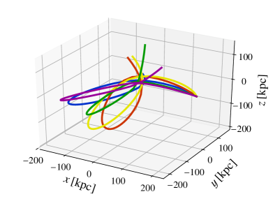
Figure 1: Visualization of the orbits (orbitI to orbitV) presented in Table 2 from infall to $5.7\,\rm Gyr$ after infall. The colour coding is the same as in Table 2.

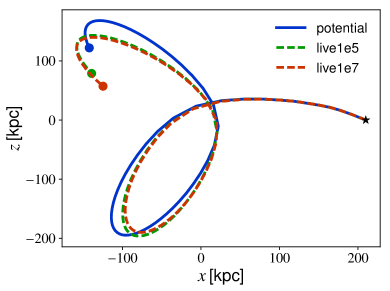
Figure 2: Projection of orbitII onto the $x-z$ plane comparing the evolution in an analytic potential (blue), in a live halo with $10^{5}$ (green) and $10^{7}$ (red) dark matter particles. A star marks the start of the orbit while the dot marks the end.

3 Results

3.1 Rotational support

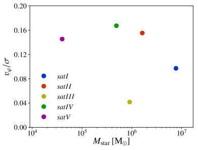
Figure 3: Amount of rotation along the axis of total stellar angular momentum of the stars compared to stellar velocity dispersion as a function of stellar mass.

One main difference between our approach and previous studies in the literature is the use of cosmological simulations as initial conditions, it is then interesting to check the dynamical state of our galaxies before the infall. In Fig. 3 we show the amount of rotational support of the stellar component in the dwarf galaxies at $z=1$. We obtain the rotational velocity $v_{\varphi}$ by averaging the individual velocities of the stellar particles in $\vec{e}_{\varphi}$ direction. The unit vector $\vec{e}_{\varphi}$ is set as the circumferential direction with respect to the axis defined by the total stellar angular momentum of stars within the half mass radius. The velocity dispersion $\sigma$ is simply given by $\sigma=\sigma_{3D}/\sqrt{3}$, where $\sigma_{3D}$ is the three dimensional velocity dispersion of the stellar particles in the half mass radius. As shown in Fig. 3 our galaxies show that there is not much rotational support and their structure can be described by a single isotropic component with practically no signs of a stellar disc even before infall. This is in agreement with previous studies which showed that in cosmological simulations isolated dwarf galaxies as well as satellite galaxies at the low mass end seem to be dispersion supported systems (Wheeler et al., 2017).

However this is quite different from several previous works studying satellite-host interaction, which usually adopted values of $v_{\mathrm{rot}}/\sigma\approx 2$ (Kazantzidis et al., 2017) with a well defined disc component, and then witness a “morphological transformation” within the host halo (Łokas et al., 2010). In our case no morphological transformation is needed since cosmological simulations seem to indicate that galaxies, on our mass scales, are already quite “messy” and do not show the presence of a stellar disc.

3.2 Environmental effects on galaxy properties

All the satellites survive till redshift $z=0$ on orbits from orbitI to orbitV with the exception of satI on orbitV, since in this case our centering algorithm is not able to find a well defined stellar (or dark matter) centre for the satellite, as it is also confirmed by a visual inspection which shows the satellite being completely destroyed. The same happens for the radial orbit scenario, in which all satellites are destroyed with no exceptions, we plan to analyze these tidal debris in a forthcoming paper. Since in this paper we are interested in the properties of “alive” satellites at $z=0$, we will therefore focus on orbitI to orbitV for all our satellites but excluding orbitV for satI.

Mass loss and abundance matching

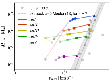
Figure 4: The stellar mass within three stellar 3D half mass radii (at infall) as a function of the maxium circular velocity. The gray band shows the Moster relation and its errors translated to a function of $v_{\mathrm{max}}$ for a concentration of $c=7$. Triangles denote the isolated simulations while the filled circles denote the different orbits. The more violent the orbit, the fainter is the colour of the dots.

In Fig. 4 we show the stellar mass within three half mass radii at infall as a function of the maximum of the total circular velocity profile $v_{\mathrm{max}}$. The half light radius is determined by the radius of a sphere around the centre of the satellite containing half of its stellar mass, we will refer to this measure as the $3D$ half mass radius. The (coloured) triangles mark the results for the isolated runs at redshift zero. The (coloured) filled circles represent the runs in the disc+halo potential, same colours refer to the same satellite (they are also connected by a line to facilitate the comparison), while the strength of the colour goes from dark to faint as the orbit becomes more destructive, i.e. from orbits (orbitI to orbitV). We will use the same colour scheme in the rest of the paper. Finally the grey circles represent the full sample of haloes presented in PaperI at $z=1$ and are only added for comparison.

The dashed grey line shows the extrapolation to low mass haloes of the abundance matching relation from (Moster et al., 2013) and its error band. Since for satellites it is hard to define the total halo mass we have translated this last quantity into a maximum circular velocity. This has been assuming a NFW potential for the total matter distribution with concentration $c=7$ (which is the average concentration of our simulated haloes) and also assuming that the maximum circular velocity occurs at the radius $r=2.16\,r_{s}$ (Bullock et al., 2001) where $r_{s}$ is the NFW scale radius.

Our galaxies started on the abundance matching relation (grey circles, see also Paper I), and they remain there when run in isolation (coloured triangles). Then depending on the orbit, they leave the relation as a consequence of tidal stripping. For quiet orbits they move almost parallel to the x-axis (i.e. with constant stellar mass), meaning that the central region of the satellite is fairly unaltered, then for more disruptive orbits also the stellar component is affected and the stellar mass can shrink to up to $1\%$ of its initial value. Overall the satellites seem to perform a characteristic curve in the stellar mass vs. maximum circular velocity plane due to tidal stripping.

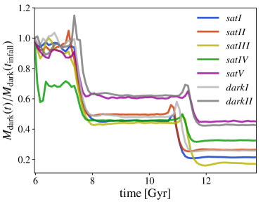
Figure 5: Evolution of the dark matter mass in terms of the dark matter mass at infall of the seven satellites on orbitII. Only the mass in $10\%$ of the virial radius at infall is considered.

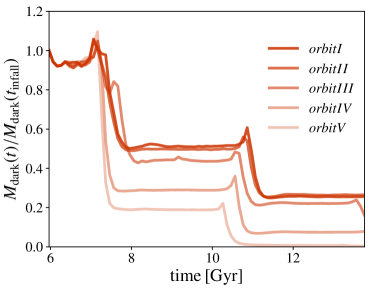
Figure 6: Evolution of the dark matter mass in terms of the dark matter mass at infall for satII on the five orbits. Only the mass in $10\%$ of the virial radius at infall is considered.

It is interesting also to look at the time evolution of the dark matter mass near the (luminous) centre of our haloes. In Fig. 5 we show the evolution of the dark matter mass enclosed in $10\%$ of the initial (at infall) virial radius for all our satellites on the same orbit, namely orbitII.

Until the first pericentre passage at $t\approx 8\,\rm Gyr$ the dark matter mass is more or less stable with the exception of satIV in which a (sub)substructure that passed nearby the centre led to an overestimation of the initial enclosed mass. During the first pericentre passage the satellites lose about half their inner dark matter mass. Then we find again a quite stable period untill the second pericentre passage at $t\approx 11\,\rm Gyr$, when the satellites are stripped again and left with $15-50\%$ of their initial dark matter mass at redshift $z=0$.

The second stripping event, corresponding to the second pericentre passage, occurs in the time range 11 to 12  Gyr for all the satellites. The more massive satellites however seem to experience this event earlier (shortly after 11  Gyr ) than the less massive ones. This implies a sort of "decay" of the orbital trajectory for more massive satellites even in the absence of dynamical friction. This can be ascribed to the different redistribution of energy and orbital angular momentum between stripped material and the satellite remnant. Finally in Fig. 6 we show the evolution of the dark matter mass this time for a single satellite (satII) on all five orbits. The fraction of dark matter remainig in the halo at redshift $z=0$ varies from $30\,\%$ on orbitI to just a few percent on orbitV.

Stellar mass assembly

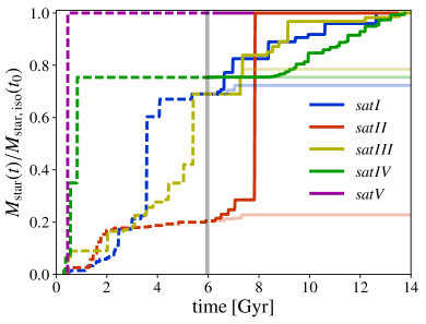
Figure 7: Evolution of the stellar mass of the 5 luminous satellites before (dashed) and after (solid) the infall time ($z=1$). Isolated runs are shown with darker colours while orbits (specifically orbitII) are shown with fainter ones. The stellar mass is shown in terms of the stellar mass at time $z=0$.

We now turn our attention to the luminous part of the satellites. The evolution of the stellar mass in the cosmolocigal simulations until redshift $z=1$ (dashed) and physical simulations (solid) is shown in Fig. 7 for the isolated run and orbitII (faint lines).

The stellar mass as a function of time is reconstructed from the formation times of the individual stellar particles. All stellar particles that remain within $10\%$ of the virial radius $r_{\mathrm{200,infall}}$ at infall at redshift $z=0$ are considered and weighted with their initial stellar mass $m_{\mathrm{star,\,init}}$. We will use the virial radius at infall as a scale for the dark matter halo during the satellite evolution and we will refer to it just as the virial radius $r_{200}$. The star formation before infall has been further investigated in (Macciò et al., 2017). The galaxies show various behaviours of star formation in isolation, from absence of star formation in satV to a starburst due to a merger with substructure in satII. On the orbit however the star formation plays no or at least a minor role.

Metallicity

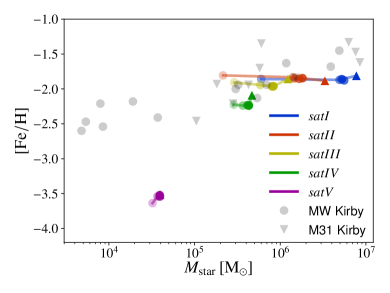
Figure 8: Metallicity as a function of the stellar mass. The coloured triangles denote the isolated simulations while the filled circles denote the different orbits. The more violent the orbit, the fainter is the colour of the dots. Observations of Milky Way and M31 satellites from (Kirby et al., 2014) are shown as grey dots and triangles, respectively.

We present the mass weighted stellar metallicity as a function of stellar mass enclosed in a sphere of three 2D half mass radii in Fig. 8. Where the 2D half mass radius is defined as the radius of a cylinder along the $z$-axis (our line-of-sight) containing half of the galaxy stellar mass.

As before the triangle marks the position of the isolated simulation, while the different coloured circles mark the results for the different orbits, with faint colours being associated with more disruptive orbits. The grey circles and triangles represent observational results for the Milky Way and the M31 galaxy respectively. Our isolated runs nicely reproduce the observational trend from Kirby et al. (2014), with the exception of satV, the apparent failure of this satellite is related to the very short time scale of star formation compared with the time-step of the simulation, which does not allow for a proper treatment of the enrichment (see PaperI for a thorough explanation of this issue).

When the satellites are exposed to the presence of a central halo, they do lose stellar mass (as expected), but they still move parallel to the relation, with an almost constant metallicity, due to the very low metal gradient in their stellar population.

Stellar kinematics

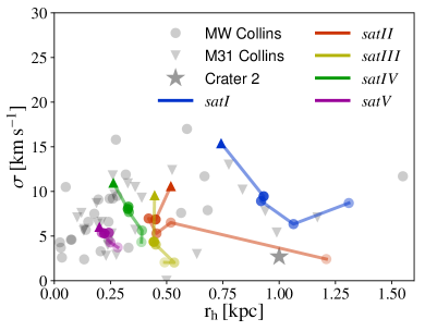
Figure 9: Projected velocity dispersion inside the stellar 2D half mass radius as a function of the stellar 2D half mass radius. coloured triangles denote the isolated simulations while the filled circles denote the different orbits. The more violent the orbit, the fainter is the colour of the dots. Observations of Milky Way and M31 satellites (for references see section 3.2) are shown as grey dots (and a star for the recently discovered satelite Crater 2) and triangles, respectively.

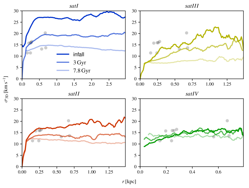
Figure 10: Three dimensional velocity dispersion of the stellar particles on orbitII evaulated at infall (solid), $3\,\rm Gyr$ and $7.8\,\rm Gyr$ ($z\approx 0$) (faint, solid). Grey points denote line of sight velocity dispersion measurements from Walker et al. (2009) of the nine most massive Milky Way satellites rescaled by a factor of $\sqrt{3}$ (Wolf et al., 2010).

The effect of accretion onto a more massive galaxy is instead clearly visible in the velocity dispersion-size relation which is shown in Fig. 9. The size ($r_{\rm h}$) is again the 2D half mass radius already introduced above, while the velocity dispersion is the 1D dispersion along the line of sight (the $z$=axis in our case) computed within $r_{\rm h}$. In this plot the observational data are represented by grey dots and triangles for Milky way and M31 satellites, respectively. They are taken from a compilation from M.Collins (private communication) including data from Walker et al. (2009) for the Milky Way and Tollerud et al. (2012); Tollerud et al. (2013); Ho et al. (2012); Collins et al. (2013); Martin et al. (2014) for M31 satellites. The size and dispersion measurements of the recently discovered satellite Crater 2 are taken from Caldwell et al. (2017).

Our isolated haloes (triangles) lie well within the relation as were our initial conditions (see Paper I). Stripping and tidal forces modify both the size and the velocity dispersion of the galaxies, which, depending on the orbit, at redshift zero tend to occupy the whole space covered by the observations.

It is interesting to note that simulated galaxies with larger sizes tend to have a larger deviation (both in size and dispersion) from the isolated runs, suggesting that small galaxies tend to be more resilient to tidal effects. Overall the scatter in our simulated size-dispersion velocity is in very good agreement with the observed one. Further we want to emphasise that satII and orbitV end up with an extremely low velocity dispersion at a half mass radius of about $1.2{\,\rm kpc}$. This is in very good agreement with the properties of the recently discovered Crater2 satellite (Caldwell et al., 2017). This implies that the formation of such extended and cold structures is not a challenge for the current LCDM model, which can be explained as highly perturbed objects (see also Munshi et al. (2017)).

To better understand the time evolution of the stellar kinematics in our satellites, in Fig. 10 we show the radial profile of the three dimensional stellar velocity dispersion on orbitII at three different times: at infall and after $3$ and $7.8\,\rm Gyr$ (corresponding to redshift $z=0$). Here we only consider satI to satIV because satV has not sufficient stellar particles to resolve the kinematics properly (see Table 1). In the same plot we also show as reference (grey circles) the line of sight velocity dispersion measurements for the nine most massive Milky Way satellites at the half light radius from Walker et al. (2009) rescaled by a factor of $\sqrt{3}$ (see Wolf et al., 2010)). As time goes by the mass (DM+stellar) loss causes an overall decrease of stellar velocity dispersion, which also tends to become more isothermal, with a very flat distribution (see for example the case for satIII) at redshift zero. We ascribe this effect to the particle phase space mixing due to tidal effects, which seems to “thermalize” the galaxy.

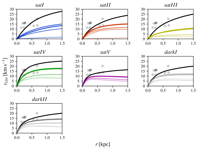
Figure 11: Circular velocity profiles for the five luminous satellites for the isolated run (black) and the orbits (colour coding as before). The more violent the orbit, the fainter is the line colour. Grey points denote line of sight velocity dispersion measurements from Walker et al. (2009) of the nine most massive Milky Way satellites rescaled by a factor of $\sqrt{3}$ (Wolf et al., 2010).

Another interesting (and measurable) quantity to look at is the circular velocity, defined as $v_{\mathrm{circ}}=\sqrt{\frac{GM(<r)}{r}}$, where $M(<r)$ is the total mass enclosed in a sphere with radius $r$ around the centre. In Fig. 11 we show the final ($z=0$) circular velocity radial profile for all our seven satellites and for different orbits. In each panel the black line represents the isolated run, while the coloured lines are the orbit runs, with, as before, fainter colours for more disruptive orbits. We also show, as in the previous figures, the observations of the nine most massive Milky Way satellites as an orientation (data from Walker et al., 2009). As already noted in previous studies, circular velocity profiles can be significantly lowered in the inner few hundred parsecs, even without losing a large amount of mass on these scales (see Fig. 4). The profiles also tend to evolve in a sort of self-similar way, preserving their initial shape, with the exception of the most extreme orbit.

3.3 Evolution of the dark matter profile

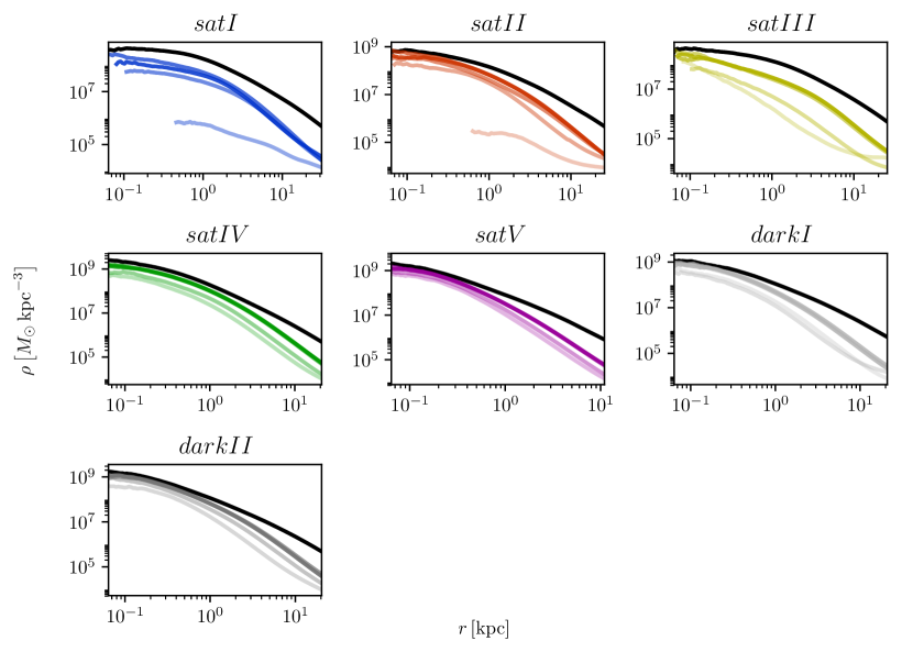
Figure 12: Dark matter density profile of all the satellites in isolation (black) and on the orbits (colour coding as before) at redshift $z=0$. The more violent the orbit, the fainter is the line colour. The profiles are shown from twice the softening length up to the virial radius at infall.

We now turn our attention to the dark (matter) component of our satellites. In Fig. 12 we show the redshift zero dark matter distribution for all our galaxies in the various runs at redshift $z=0$, as before the black line represents the isolation run, while the coloured lines are for the different orbits. The profiles are shown from twice the gravitational dark matter softening to the virial radius at infall (the exceptions are satellites satI, satII and satIII on the most extreme orbit, since they end up with a very low dark matter content at $z=0$ and which pushes the convergence radius to larger scales). As expected the tidal stripping due to the central potential is stronger in the outer parts of the profile, which depart more from the isolation case. On the other hand the stripping does not happen in an “onion-like” fashion, with the outer part being progressively removed while the centre remains unaltered. On the contrary, the whole profile reacts to the stripping and the central density is also lowered even on the most mild orbits. This global reaction can be ascribed to the typical box orbits of dark matter particles (e.g. Bryan et al., 2012), which allow particles in the centre at a given time step, to spend quite some time in the outskirts of the halo at a subsequent time, and hence are prone to be stripped.

As already described in PaperI, some of our satellites (satI, satII, satIII as shown by the isolation runs) start with a cored dark matter profile (or at least a profile with a shallower slope than NFW), this is due to the fact that for those satellites, the star formation rate is vigorous enough to create large gas outflows, which in turn flatten the dark matter profile (Read & Gilmore, 2005; Pontzen & Governato, 2012; Macciò et al., 2012b; Di Cintio et al., 2014; Oñorbe et al., 2015). Fig. 12 seems to suggest a steepening of the profile during its evolution. To better look into this possibility we plot in Fig. 13 the inner logarithmic dark matter density slope $\alpha$ as a function of stellar mass. The slope $\alpha$ is computed between 1-2% of the initial (at infall) virial radius, following Tollet et al. (2016) and PaperI; the triangles mark the isolation runs, while the circles represent the different orbits, finally the stellar mass for the two dark haloes has been arbitrarily set.

No matter if the halo contained stars or not, or whether it starts with a flattened profile (blue and yellow symbols) or with a cuspy one (green symbols), in all cases the effect of accretion is to steepen the dark matter profile. It is important to notice that the profile steepening is not due to a contraction of the halo but it is due to a slightly stronger mass removal in the outer regions of the halo with respect to its very centre.

In Fig. 12 we do not show the final density profile slope for satI (blue), satII (red) and satIII (yellow) for the most extreme orbit. This is because at $z=0$ these satellites do not have a clear dark matter centre to build the profile. It is nevertheless interesting to look at the evolution of the dark matter profile as a function of time before the satellite disruption. This is shown in Fig. 14 where we present the difference of the density slope $\alpha$ w.r.t. to the isolation case as a function of time: the plots show satI (blue line), satII (red line) and satIII (yellow line) on orbitIV (for satI) and orbitV (for satII and satIII), respectively, and the profile slopes are averaged over five time-steps to reduce the noise. It is evident that the steepening of the profile is present even for satellites that are completely shredded apart by tidal forces.

When the results of PaperI and this work are combined, they imply that the observational discovery of a dark matter core in one of the low mass satellites of our own Galaxy will strongly challenge the predictions of the $\Lambda{\rm CDM}$ model. It will be very difficult to explain such dark matter core invoking the effect of baryons (Paper I and triangles in Fig. 13) or the effect of environment and accretion (again Fig. 13). The discovery of a flat dark matter distribution will then be an indication of a different nature for dark matter: warm (but see Macciò et al., 2012a), self interacting (Vogelsberger et al., 2014b; Elbert et al., 2015) or even more exotic models (e.g. Macciò et al., 2015).

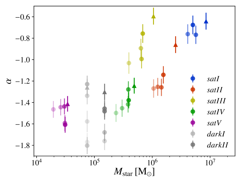
Figure 13: Inner logarithmic slope of the dark matter density profile $\alpha$ fitted between $1\%$ and $2\%$ of the virial radius as a function of stellar mass inside three 3D half mass radii. Stars denote measurements at infall, while triangles denote the isolated simulations and filled circles the orbit runs at redshift $z=0$. The more violent the orbit, the fainter is the colour.

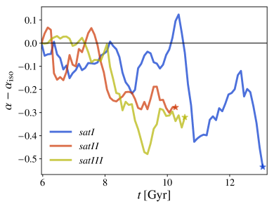
Figure 14: Time evolution of the deviation of $\alpha$ on orbitIV and orbitV from $\alpha_{\mathrm{iso}}$ (for the isolated runs) for satI, satII and satIII, respectively. The stars denote the time where there are less than $150$ dark matter particles left inside a sphere of a radius of $1\%\,r_{200}$.

3.4 Central dark matter density slope and satellite survival

Previous works studying environmental effects on satellite galaxies (e.g. Kazantzidis et al., 2004a; Peñarrubia et al., 2010, and references therein) have shown that satellites with cored dark matter density profiles are more easily stripped and disrupted than cuspy ones. The results shown in Fig. 13 seemed to confirm such a correlation also in our cosmologically based simulations, but we want to be more quantitative.

In Fig. 15 we show the ratio of the dark matter enclosed within three half mass radii for the different satellites on the different orbits with respect to the isolated case as a function of the initial (at infall) density profile slope at redshift $z=0$. It is quite evident that on every orbit, cuspy satellites like satV ($\alpha_{\rm infall}=-1.5$) are able to retain a larger fraction of their initial mass than cored ($\alpha_{\rm infall}>-1.0$ ) satellites like satI and satIII. These cored satellites lose more than 70% of their initial (dark) mass even on the more gentle orbit (darker colours) and up to almost 100% on the most extreme ones (fainter colours).

The different initial dark matter density slope also affects the stellar mass loss, since the dark matter acts as shield for the stars. In Fig. 16 we plot the mass loss as defined in Fig. 15 as function of the initial dark matter profile density slope but this time for stars and dark matter. In order to avoid a too crowded plot we only show results for orbitIV, which is the most disruptive orbit for which all five satellites still have a well defined centre.

In general stars are more resilient to tidal forces than dark matter, and this is due to their smaller spatial extent and larger stellar density; for example satIII is able to retain 40$\%$ of its stars while it is practically totally stripped of dark matter. Nevertheless there is still a correlation between the stellar mass loss and the initial dark matter slope. An exception to this relation seems to be given by satI, which has a very strong mass loss both in the stellar and dark matter components despite having a similar $\alpha_{\rm infall}$ as satIII. This is due to the different slope for the stellar density profiles between satI and satIII, while the first satellite has a slope of $-1.80$ (again evaluated between 1 and $2\%$ of the virial radius), the stellar slope for satIII (and all the other satellites) it is close to $-3.0$. This difference in stellar slope is most likely related to a major merger event that occurred for satI shortly before redshift one and strongly reshuffled the stellar particle orbits.

Finally we note that some satellites (especially satI) are left at $z=0$ with practically no dark matter in their central region, where they are fully stellar dominated, resembling more an extended globular cluster than a dwarf galaxy, we plan to look more into this issue in a forthcoming paper.

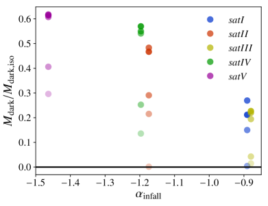
Figure 15: Dark matter mass enclosed in a constant sphere with a radius of three stellar half mass radii at infall on the individual orbits compared to the isolated run as a function of the central dark matter density slope at infall $\alpha_{\mathrm{infall}}$.

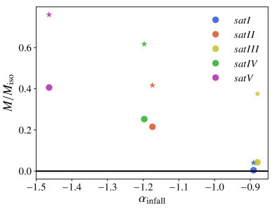
Figure 16: Dark matter (dots) and stellar (stars) mass enclosed in a constant sphere with a radius of three stellar half mass radii at infall on orbitIV compared to the isolated run as a function of the central dark matter density slope at infall $\alpha_{\mathrm{infall}}$.

4 Discussion and Conclusions

This work is the second of a series of papers in which we are trying to understand the formation and evolution of the smallest galaxies in the universe.

In the first paper (Macciò et al., 2017) we presented a series of 27 cosmological simulations of halos in the mass range $5\times 10^{8}$ to $10^{10}\,$ ${\rm M}_{\astrosun}$ , these simulations were run till $z=1$ and aimed to describe the properties of satellite galaxies before accretion.

In this second paper we used a subsample of these cosmological simulations as initial conditions for a series of binary hydrodynamical simulations (satellite + host) with the goal of understanding the effects of accretion and environment on satellite galaxies.

More specifically we used a total of seven haloes (5 luminous and 2 dark) with a virial mass in the range $4\times 10^{9}$ to $10^{10}{\rm M}_{\astrosun}$. We modeled the central halo with an analytic potential of halo (NFW) plus disc (Miyamoto & Nagai), and we run the simulations from redshift one until redshift zero. We use five different orbits (plus a radial orbit) for a total of 42 simulations. Each galaxy is also evolved “in isolation” meaning without the presence of the central halo for the same amount of time as our “orbit” runs. We also add an analytic model for ram pressure and we test the results of our analytic potential against a live halo.

We find that our cosmological initial conditions differ from model (pre cooked) galaxies in their kinematics: our galaxies, even before accretion do not have a well defined rotating stellar disc and are dispersion supported, with an average value of $v_{\varphi}/\sigma$ of 0.14, and as low as 0.04.

While orbiting around the central host, all galaxies lose a considerable fraction of their halo mass, as a consequence they drift away from the widely used abundance matching relations, due to a reshuffling of the mass rank order of the satellites. Only the more extreme orbits, with small pericentre distances are effective in stripping the stellar component too, and the stripping is substantial only for our most massive (and extended) galaxies. Star formation is strongly suppressed after the infall (in comparison with the isolation run), this happens regardless of the presence or absence of ram pressure.

The environment has different effects on different scaling relations. In the stellar mass - metallicity plane, galaxies, even when they lose stellar mass, tend to keep an almost constant metallicity, due to the lack of strong metallicity gradients in the galaxy. In the size - velocity dispersion relation, galaxies move substantially in all directions, depending on their orbits and initial size. Galaxies tend to become more extended and to reduce their velocity dispersion (due to dark matter stripping). This explains the overall large observed scatter in the $r-\sigma$ plane.

Finally the interaction with the host leads to a flattening of the stellar velocity dispersion profiles of the satellites, possibly due to the potential perturbation redistributing the stellar orbits into a more “thermalized” system.

The dark matter component is also very strongly perturbed, first of all the removal of particles from the outer part of the halos does not happen in an “onion-like” fashion, with the external layers removed first. The whole density profile reacts to the accretion and even the most internal regions are affected by mass removal even if at a lower degree of the external ones. This implies an overall suppression of the circular velocity curves with respect to the isolation runs, even in the central part.

We find a correlation between the initial (at infall) inner dark matter density slope and the efficiency of mass removal and satellite survival that is in good agreement with previous studies. Cored satellites are less resilient to stripping and tidal forces and are more prone to lose a very large fraction of their dark matter mass (if not all of it) on orbits with close pericentre passages. Some cored satellites are so heavily stripped in their dark matter component that they end up being almost entirely stellar dominated within three stellar half mass radii. Stars are also more easily stripped when embedded in a halo with a flat density profile, even though to a lower extent.

We witness a steepening of the central slope of the dark matter profile during accretion, with more extreme orbits ending up with the most cuspy dark matter profiles. Even profiles that initially (before accretion) have a dark matter density profile shallower than NFW (due to baryonic effects) evolve into cuspy profiles with slopes consistent with pure N-body simulations when set on orbits with small pericenter passages (7-20 kpc). Interestingly also our dark haloes (without stars) do steepen their profiles.

Overall our simulations seem to make a quite clear prediction of steep dark matter profiles for objects at the edge of galaxy formation, a prediction that, if falsified by observations, can force us to reconsider the collision-less and cold nature of dark matter.

References

- Aumer et al. (2013) Aumer M., White S. D. M., Naab T., Scannapieco C., 2013, MNRAS, 434, 3142
- Blumenthal et al. (1984) Blumenthal G. R., Faber S. M., Primack J. R., Rees M. J., 1984, Nature, 311, 517
- Boylan-Kolchin et al. (2011) Boylan-Kolchin M., Bullock J. S., Kaplinghat M., 2011, MNRAS, 415, L40
- Bryan et al. (2012) Bryan S. E., Mao S., Kay S. T., Schaye J., Dalla Vecchia C., Booth C. M., 2012, MNRAS, 422, 1863
- Bullock et al. (2001) Bullock J. S., Kolatt T. S., Sigad Y., Somerville R. S., Kravtsov A. V., Klypin A. A., Primack J. R., Dekel A., 2001, MNRAS, 321, 559
- Caldwell et al. (2017) Caldwell N., et al., 2017, ApJ, 839, 20
- Chan et al. (2015) Chan T. K., Kereš D., Oñorbe J., Hopkins P. F., Muratov A. L., Faucher-Giguère C.-A., Quataert E., 2015, MNRAS, 454, 2981
- Chang et al. (2013) Chang J., Macciò A. V., Kang X., 2013, MNRAS, 431, 3533
- Collins et al. (2013) Collins M. L. M., et al., 2013, ApJ, 768, 172
- D’Onghia et al. (2009) D’Onghia E., Besla G., Cox T. J., Hernquist L., 2009, Nature, 460, 605
- Di Cintio et al. (2014) Di Cintio A., Brook C. B., Macciò A. V., Stinson G. S., Knebe A., Dutton A. A., Wadsley J., 2014, MNRAS, 437, 415
- Dutton & Macciò (2014) Dutton A. A., Macciò A. V., 2014, MNRAS, 441, 3359
- Dutton et al. (2016) Dutton A. A., Macciò A. V., Frings J., Wang L., Stinson G. S., Penzo C., Kang X., 2016, MNRAS, 457, L74
- Elbert et al. (2015) Elbert O. D., Bullock J. S., Garrison-Kimmel S., Rocha M., Oñorbe J., Peter A. H. G., 2015, MNRAS, 453, 29
- Flores & Primack (1994) Flores R. A., Primack J. R., 1994, ApJ, 427, L1
- Garrison-Kimmel et al. (2017) Garrison-Kimmel S., et al., 2017, preprint, (arXiv:1701.03792)
- Grand et al. (2017) Grand R. J. J., et al., 2017, MNRAS, 467, 179
- Haardt & Madau (2012) Haardt F., Madau P., 2012, ApJ, 746, 125
- Ho et al. (2012) Ho N., et al., 2012, ApJ, 758, 124
- Hopkins et al. (2014) Hopkins P. F., Kereš D., Oñorbe J., Faucher-Giguère C.-A., Quataert E., Murray N., Bullock J. S., 2014, MNRAS, 445, 581
- Kang & van den Bosch (2008) Kang X., van den Bosch F. C., 2008, ApJ, 676, L101
- Kannan et al. (2014) Kannan R., Stinson G. S., Macciò A. V., Brook C., Weinmann S. M., Wadsley J., Couchman H. M. P., 2014, MNRAS, 437, 3529
- Kazantzidis et al. (2004a) Kazantzidis S., Mayer L., Mastropietro C., Diemand J., Stadel J., Moore B., 2004a, ApJ, 608, 663
- Kazantzidis et al. (2004b) Kazantzidis S., Kravtsov A. V., Zentner A. R., Allgood B., Nagai D., Moore B., 2004b, ApJ, 611, L73
- Kazantzidis et al. (2017) Kazantzidis S., Mayer L., Callegari S., Dotti M., Moustakas L. A., 2017, ApJ, 836, L13
- Kirby et al. (2014) Kirby E. N., Bullock J. S., Boylan-Kolchin M., Kaplinghat M., Cohen J. G., 2014, MNRAS, 439, 1015
- Klypin et al. (1999) Klypin A., Kravtsov A. V., Valenzuela O., Prada F., 1999, ApJ, 522, 82
- Knollmann & Knebe (2011) Knollmann S. R., Knebe A., 2011, AHF: Amiga’s Halo Finder (ascl:1102.009)
- Komatsu et al. (2011) Komatsu E., et al., 2011, ApJS, 192, 18
- Łokas et al. (2010) Łokas E. L., Kazantzidis S., Klimentowski J., Mayer L., Callegari S., 2010, ApJ, 708, 1032
- Macciò et al. (2012a) Macciò A. V., Paduroiu S., Anderhalden D., Schneider A., Moore B., 2012a, MNRAS, 424, 1105
- Macciò et al. (2012b) Macciò A. V., Stinson G., Brook C. B., Wadsley J., Couchman H. M. P., Shen S., Gibson B. K., Quinn T., 2012b, ApJ, 744, L9
- Macciò et al. (2015) Macciò A. V., Mainini R., Penzo C., Bonometto S. A., 2015, MNRAS, 453, 1371
- Macciò et al. (2017) Macciò A. V., Frings J., Buck T., Penzo C., Dutton A. A., Blank M., Obreja A., 2017, preprint, (arXiv:1707.01106)
- Marinacci et al. (2014) Marinacci F., Pakmor R., Springel V., 2014, MNRAS, 437, 1750
- Martin et al. (2014) Martin N. F., et al., 2014, ApJ, 793, L14
- Mayer et al. (2006) Mayer L., Mastropietro C., Wadsley J., Stadel J., Moore B., 2006, MNRAS, 369, 1021
- Miyamoto & Nagai (1975) Miyamoto M., Nagai R., 1975, PASJ, 27, 533
- Moore (1994) Moore B., 1994, Nature, 370, 629
- Moster et al. (2013) Moster B. P., Naab T., White S. D. M., 2013, MNRAS, 428, 3121
- Moster et al. (2014) Moster B. P., Macciò A. V., Somerville R. S., 2014, MNRAS, 437, 1027
- Munshi et al. (2017) Munshi F., Brooks A. M., Applebaum E., Weisz D. R., Governato F., Quinn T. R., 2017, preprint, (arXiv:1705.06286)
- Navarro et al. (1996) Navarro J. F., Frenk C. S., White S. D. M., 1996, ApJ, 462, 563
- Oñorbe et al. (2015) Oñorbe J., Boylan-Kolchin M., Bullock J. S., Hopkins P. F., Kereš D., Faucher-Giguère C.-A., Quataert E., Murray N., 2015, MNRAS, 454, 2092
- Oh et al. (2015) Oh S.-H., et al., 2015, AJ, 149, 180
- Peñarrubia et al. (2010) Peñarrubia J., Benson A. J., Walker M. G., Gilmore G., McConnachie A. W., Mayer L., 2010, MNRAS, 406, 1290
- Peebles (1984) Peebles P. J. E., 1984, ApJ, 277, 470
- Penzo et al. (2014) Penzo C., Macciò A. V., Casarini L., Stinson G. S., Wadsley J., 2014, MNRAS, 442, 176
- Perlmutter et al. (1999) Perlmutter S., et al., 1999, ApJ, 517, 565
- Pontzen & Governato (2012) Pontzen A., Governato F., 2012, MNRAS, 421, 3464
- Power et al. (2003) Power C., Navarro J. F., Jenkins A., Frenk C. S., White S. D. M., Springel V., Stadel J., Quinn T., 2003, MNRAS, 338, 14
- Read & Gilmore (2005) Read J. I., Gilmore G., 2005, MNRAS, 356, 107
- Riess et al. (1998) Riess A. G., et al., 1998, AJ, 116, 1009
- Sawala et al. (2016) Sawala T., et al., 2016, MNRAS, 457, 1931
- Schaye et al. (2015) Schaye J., et al., 2015, MNRAS, 446, 521
- Shen et al. (2010) Shen S., Wadsley J., Stinson G., 2010, MNRAS, 407, 1581
- Springel et al. (2005) Springel V., Di Matteo T., Hernquist L., 2005, MNRAS, 361, 776
- Stinson et al. (2006) Stinson G., Seth A., Katz N., Wadsley J., Governato F., Quinn T., 2006, MNRAS, 373, 1074
- Stinson et al. (2013) Stinson G. S., Brook C., Macciò A. V., Wadsley J., Quinn T. R., Couchman H. M. P., 2013, MNRAS, 428, 129
- Tollerud et al. (2012) Tollerud E. J., et al., 2012, ApJ, 752, 45
- Tollerud et al. (2013) Tollerud E. J., Geha M. C., Vargas L. C., Bullock J. S., 2013, ApJ, 768, 50
- Tollet et al. (2016) Tollet E., et al., 2016, MNRAS, 456, 3542
- Vogelsberger et al. (2014a) Vogelsberger M., et al., 2014a, MNRAS, 444, 1518
- Vogelsberger et al. (2014b) Vogelsberger M., Zavala J., Simpson C., Jenkins A., 2014b, MNRAS, 444, 3684
- Wadsley et al. (2004) Wadsley J. W., Stadel J., Quinn T., 2004, Nature, 9, 137
- Walker et al. (2009) Walker M. G., Mateo M., Olszewski E. W., Peñarrubia J., Wyn Evans N., Gilmore G., 2009, ApJ, 704, 1274
- Wang et al. (2015) Wang L., Dutton A. A., Stinson G. S., Macciò A. V., Penzo C., Kang X., Keller B. W., Wadsley J., 2015, MNRAS, 454, 83
- Wetzel et al. (2016) Wetzel A. R., Hopkins P. F., Kim J.-h., Faucher-Giguère C.-A., Kereš D., Quataert E., 2016, ApJ, 827, L23
- Wheeler et al. (2017) Wheeler C., et al., 2017, MNRAS, 465, 2420
- White & Rees (1978) White S. D. M., Rees M. J., 1978, MNRAS, 183, 341
- Wolf et al. (2010) Wolf J., Martinez G. D., Bullock J. S., Kaplinghat M., Geha M., Muñoz R. R., Simon J. D., Avedo F. F., 2010, MNRAS, 406, 1220