Chaos and predictability of homogeneous-isotropic turbulence

Abstract

We study the chaoticity and the predictability of a turbulent flow on the basis of high-resolution direct numerical simulations at different Reynolds numbers. We find that the Lyapunov exponent of turbulence, which measures the exponential separation of two initially close solution of the Navier-Stokes equations, grows with the Reynolds number of the flow, with an anomalous scaling exponent, larger than the one obtained on dimensional grounds. For large perturbations, the error is transferred to larger, slower scales where it grows algebraically generating an “inverse cascade” of perturbations in the inertial range. In this regime our simulations confirm the classical predictions based on closure models of turbulence. We show how to link chaoticity and predictability of a turbulent flow in terms of a finite size extension of the Lyapunov exponent.

The strong chaoticity of turbulence does not spoil completely its predictability. Such apparent paradox is related to the hierarchy of timescales in the dynamics of turbulence which ranges from the fastest Kolmogorov time to the slowest integral time.

Ruelle argued many years ago that the growth of infinitesimal perturbations in turbulence is ruled by the fastest timescale Ruelle (1979). This leads to the prediction that the Lyapunov exponent is proportional to the inverse of the Kolmogorov time, and hence it increases with the Reynolds number. Turbulent flows at high $Re$ are therefore strongly chaotic Deissler (1986). Nonetheless, the time that it takes for a small perturbation to affect significantly the dynamics of the large scales is expected to be of the order of the slow integral time Lorenz (1969). The ratio between these extreme timescales increases with the Reynolds number and therefore allows a finite predictability time to coexist with strong chaos Boffetta et al. (2002). This is evident from everyday experience: while the Kolmogorov time of the atmosphere (in the planetary boundary layer) is a fraction of a second Garratt (1992) the weather is predictable for days.

The study of the predictability problem in turbulence dates back to the pioneering works of Lorenz Lorenz (1969) and of Leith and Kraichnan Leith (1971); Leith and Kraichnan (1972). The main idea of those studies is that a finite perturbation at a given scale in the inertial range of turbulence grows with the characteristic time at that scale. Therefore, while an infinitesimal perturbation is expected to grow exponentially fast, finite perturbations grow only algebraically in time, making the predictability of the flow much longer. These ideas were applied to the predictability of decaying turbulence Métais and Lesieur (1986), two-dimensional turbulence Kida et al. (1990); Boffetta and Musacchio (2001) and three-dimensional turbulence at moderate Reynolds numbers Kida and Ohkitani (1992).

In this letter we investigate, on the basis of high-resolution direct numerical simulations, chaos in homogeneous-isotropic turbulence by measuring the growth of the separation between two realizations starting from very close initial conditions. In the limit of infinitesimal separation we compute the leading Lyapunov exponent of the flow (the rate of exponential growth of the separation Ott (2002)) and we find that it increases with the Reynolds number, but surprisingly faster than what predicted on dimensional grounds Ruelle (1979) and what observed in low-dimensional models of turbulence Crisanti et al. (1993). For larger separation we observe the transition to an algebraic growth of the error, in agreement with the predictions of closure models Leith and Kraichnan (1972). Finally, we discuss the relation between chaoticity and the predictability time of turbulence (defined as the average time for the perturbation to reach a given threshold) in terms of the finite-size generalization of the Lyapunov exponents.

We consider the dynamics of an incompressible velocity field ${\bm{u}}({\bm{x}},t)$ given by the Navier-Stokes equations

$$\partial_{t}{\bm{u}}+{\bm{u}}\cdot{\bm{\nabla}}{\bm{u}}=-\bm{\bm{\nabla}}P+\nu\Delta{\bm{u}}+{\bm{f}}\;,$$ (1)

where $P$ is the pressure field and $\nu$ is the kinematic viscosity of the fluid. The term ${\bm{f}}$ represents a mechanical forcing needed to sustain the flow. In the following we will present results in which ${\bm{f}}$ is a deterministic forcing with imposed energy input Machiels (1997); Lamorgese et al. (2005). The Navier-Stokes is solved numerically by a fully parallel pseudo-spectral code in a cubic box of size $\mathcal{L}$ at resolution $N^{3}$ with periodic boundary conditions in the three directions. The main parameters of the simulations are reported in Table 1 and further details are found in the Supplementary Material.

In presence of forcing and dissipation, the turbulent flow reaches a statistically steady state in which the energy dissipation rate $\varepsilon=\nu\langle(\partial_{\alpha}u_{\beta})^{2}\rangle$ is equal to the input of energy provided by the forcing (brackets indicate average over the physical space). The turbulent state is characterized by a Kolmogorov energy spectrum $E(k)=C\varepsilon^{2/3}k^{-5/3}$. The kinetic energy $E=\int E(k)dk=(1/2)\langle|{\bm{u}}|^{2}\rangle$ fluctuates around a constant mean value, which defines the typical intensity of the large scale flow $U=(2E/3)^{1/2}$. The integral time is defined as $T=E/\varepsilon$ and the integral scale is $L=UT$.

We performed a series of simulations at increasing Reynolds number $Re=UL/\nu$. In order to ensure that the viscous range is resolved with the same accuracy in all the simulations, the increase of $Re$ as been achieved by increasing the resolution $N$ and reducing the viscosity in order to keep fixed $k_{max}\eta=1.7$, where $k_{max}=N/3$ is the maximum resolved wavenumber and $\eta=(\nu^{3}/\varepsilon)^{1/4}$ is the Kolmogorov scale.

$N$	$Re$	$E$	$U$	$L$	$\eta$	$\tau_{\eta}$	$\lambda$
$1024$	$8224$	$0.700$	$0.683$	$4.78$	$0.005$	$0.063$	$2.72$
$512$	$3062$	$0.678$	$0.672$	$4.56$	$0.01$	$0.10$	$1.39$
$256$	$1170$	$0.665$	$0.666$	$4.43$	$0.02$	$0.16$	$0.76$
$128$	$434$	$0.643$	$0.655$	$4.21$	$0.04$	$0.25$	$0.44$

Table 1: Parameters of the simulations. For all the simulations the energy input is $\varepsilon=0.1$, and the box size is $\mathcal{L}=2\pi$. $N$ is the grid resolution, $Re=UL/\nu$ the Reynolds number, $E$ the kinetic energy, $U=(2E/3)^{1/2}$ is the large-scale velocity, $L=UE/\varepsilon$ the integral scale, $\eta=(\nu^{3}/\varepsilon)^{1/4}$ the Kolmogorov scale, $\tau_{\eta}=(\nu/\varepsilon)^{1/2}$ the Kolmogorov time and $\lambda$ the Lyapunov exponent.

For the study of chaos and predictability we are interested in measuring the growth of an uncertainty in the velocity field. Starting from an initial velocity field ${\bm{u}}_{1}({\bm{x}},0)$ in the stationary turbulent state, we generate a perturbed velocity field ${\bm{u}}_{2}({\bm{x}},0)$, obtained by adding to the reference field a small white noise (the relative amplitude of the perturbation is $O(10^{-4})$). We consider very small initial perturbations in order to guarantee that the separation between the two realizations is along the most unstable direction in phase space when the error enters in the non-linear stage and therefore we do not consider the effect of the distribution of the initial error on the predictability of the flow Hayashi et al. (2013). The two realizations of the velocity field are then simultaneously evolved in time according to (1). For each resolution, we performed an average over several independent realizations.

A natural measure of the uncertainty is the error energy $E_{\Delta}(t)$ and the error energy spectrum $E_{\Delta}(k,t)$, defined on the basis of the error field $\delta{\bm{u}}\equiv({\bm{u}}_{2}-{\bm{u}}_{1})/\sqrt{2}$ as

$$E_{\Delta}(t)=\int_{0}^{\infty}E_{\Delta}(k,t)dk={1\over 2}\langle|\delta{\bm{u}}({\bm{x}},t)|^{2}\rangle\;.$$ (2)

With the normalization coefficient $1/\sqrt{2}$ we have $E_{\Delta}=E$ for completely uncorrelated fields.

Figure 1 shows the time evolution of the error energy $E_{\Delta}$ for the simulation at the highest $Re$, averaged over an ensemble of $10$ independent realizations. In the initial stage the error grows exponentially as $E_{\Delta}(t)=E_{\Delta}(0)\exp(L_{2}t)$ (see inset of Fig. 1) where $L_{2}$ is the generalized Lyapunov exponent of order $2$ Cencini et al. (2010). At later times we observe a regime of linear growth of the error $E_{\Delta}(t)\simeq\varepsilon t$. The growth rate displays large fluctuations as the error approaches its saturation value $E_{\Delta}(t)\simeq E$. This is due to the fluctuations of the kinetic energy which occur on the same time scale of the saturation of the error and are associated to the dynamics of the large scales. It is worth to notice that the late regime of saturation of the error might display a non-universal behavior with respect to the forcing mechanism. As an example, the deterministic force used in our study is proportional to the large-scale velocity. At late times, when the error has significantly affected the large scales, the force acting on the two fields ${\bm{u}}_{1}$ and ${\bm{u}}_{2}$ becomes different. This could induce a faster saturation of the error with respect to other forcing mechanism which enforce large-scale correlations.

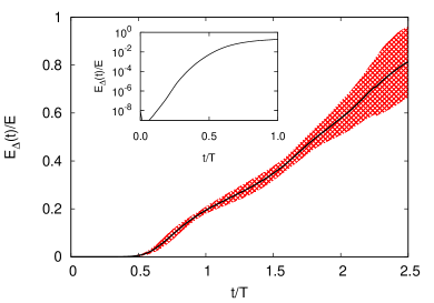
Figure 1: (Color online) Error energy $E_{\Delta}(t)$ growth for the simulation at $N=1024$. The error energy is averaged over $10$ different realizations (black line). The fluctuations of the error energy within one standard deviation from the mean are represented by the shaded area. Inset: The initial exponential growth of the error.

During the initial stage of exponential growth the error energy spectrum $E_{\Delta}(k,t)$ is peaked at wavenumbers around the dissipation range $k\simeq k_{\eta}\simeq 1/\eta$ and grows exponentially in a self similar way, as shown in Fig. 2.

At later times, the error propagates to lower wavenumbers and the error spectrum develops a scaling range $E_{\Delta}(k)\sim k^{-5/3}$ (see Fig. 3). At each time it is possible to identify the error wavenumber $k_{E}(t)$ at which the error energy spectrum has reached a given fraction $\alpha\simeq 1$ of the energy spectrum $E_{\Delta}(k_{E},t)/E(k_{E})=\alpha$. The two velocity fields ${\bm{u}}_{1}$ and ${\bm{u}}_{2}$ can be then assumed to be completely decorrelated at scales smaller than $1/k_{E}$ and still correlated at larger scales.

Figure 2: The spectrum of the error $E_{\Delta}(k,t)$ at times $t/T=0.07,0.14,0.21,0.28,0.35$ (from bottom to top) in the linear phase for the simulation at $N=1024$ averaged over $10$ independent realizations. Inset: The error energy $E_{\Delta}$ as a function of time in semilogarithmic plot.

Figure 3: The spectrum of the error $E_{\Delta}(k,t)$ at times $t/T=0.42,0.56,0.70,0.84,1.1,1.4,1.8,2.1$ (dashed lines, from bottom to top) compared with the stationary energy spectrum $E(k)$ (solid line) for simulations at $N=1024$ averaged over $10$ independent realizations. The dotted line represents the Kolmogorov scaling $k^{-5/3}$. Inset: The error wavenumber $k_{E}$ as a function of time (crosses), compared with the dimensional scaling $k_{E}\sim t^{3/2}$ (dotted line).

The transition from the exponential growth to the linear growth of $E_{\Delta}$ occurs when the two fields are completely decorrelated on the dissipative scales, that is when $k_{E}\simeq k_{\eta}$ . The idea, originally proposed by Lorenz Lorenz (1969), is that the time that it takes to decorrelate completely the two fields at a given scale $\ell\simeq 1/k$ within the inertial range is proportional to the turnover time of the eddies at that scale $\tau_{\ell}\sim\varepsilon^{-1/3}\ell^{2/3}$ Frisch (1995). This leads to the dimensional prediction

$$k_{E}(t)\simeq\varepsilon^{-1/2}t^{-3/2}$$ (3)

for the evolution of the error wavenumber, which is confirmed by our numerical finding (see inset of Fig. 2).

Equation (3) provides an estimation of the predictability time $T_{P}$ that an infinitesimal error takes to contaminate a given wavenumber $k$, $T_{p}(k)=A\varepsilon^{-1/3}k^{-2/3}$ Leith and Kraichnan (1972); Cardesa et al. (2015) where the dimensionless coefficient $A$ depends on the threshold $\alpha$ (and possibly on the Reynolds number). In our simulation at $Re=8516$ we measure $A=12$ for $\alpha=0.5$ to be compared with the value $A=10$ obtained from early studies with closure models in the limit of infinite $Re$ Leith and Kraichnan (1972).

Integrating the error spectrum with the ansatz $E_{\Delta}(k,t)=0$ for $k<k_{E}(t)$ $E_{\Delta}(k,t)=E(k)$ for $k>k_{E}(t)$ and using the dimensional scaling (3), one obtains the prediction for the linear growth of the error energy:

$$E_{\Delta}(t)=G\varepsilon t\;.$$ (4)

The value of the dimensionless constant $G$ measured in the simulation at $Re=8516$ is $G=0.45\pm 0.05$, not far from that obtained by the test field model closure $G=0.23$ Leith and Kraichnan (1972).

As already discussed, in the early stage the perturbation can be considered infinitesimal and therefore grows exponentially as shown in the inset of Fig. 1. This is the signature of the chaotic nature of the flow and the predictability is characterized by the Lyapunov exponent $\lambda$. On dimensional grounds the Lyapunov exponent can be assumed to be proportional to the inverse of the fastest time-scale of the flow, i.e., the Kolmogorov timescale $\tau_{\eta}=(\nu/\varepsilon)^{1/2}$ Ruelle (1979). Since the ratio between $\tau_{\eta}$ and the integral timescale $T$ increases with the Reynolds number as $T/\tau_{\eta}\sim Re^{1/2}$ one has the prediction that the Lyapunov exponent is proportional to the square root of the Reynolds number:

$$\lambda\simeq\tau_{\eta}^{-1}\simeq T^{-1}Re^{1/2}\;.$$ (5)

Therefore the predictability time $T_{P}$ for infinitesimal perturbations vanishes in the limit of large $Re$.

The dimensional prediction (5) is obtained under the assumption of self-similarity of the velocity field with Kolmogorov scaling exponent $h=1/3$ Frisch (1995) For a generic exponent $h\in(0:1)$ one has $\lambda\simeq\tau_{\eta}^{-1}\simeq T^{-1}Re^{\beta}$ with $\beta=(1-h)/(1+h)$. Averaging over the multifractal spectrum $\mathcal{D}(h)$ allows to take into account intermittency corrections and this gives $\beta=0.459$ Crisanti et al. (1993); Aurell et al. (1996).

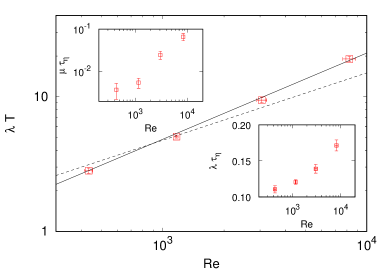
Figure 4: (Color online) Lyapunov exponents $\lambda$ as a function of $Re$ (squares). The solid line represents the best fit scaling $\lambda T\simeq Re^{0.64}$ while the dashed line is the dimensional scaling $\lambda T\simeq Re^{1/2}$. Lower inset: The Lyapunov exponents $\lambda$ compensated with the Kolmogorov time scale $\tau_{\eta}$ as a function of $Re$. Upper inset: The Lyapunov variance $\mu$ compensated with the Kolmogorov time scale $\tau_{\eta}$ as a function of $Re$.

We have computed the Lyapunov exponent $\lambda$ by measuring the average rate of logarithmic divergence of two close realizations, a standard method in the study of dynamical systems Benettin et al. (1976, 1980); Cencini et al. (2010), for the simulations at different Reynolds numbers (see Table 1). Interestingly, we find that the Lyapunov exponent increases with $Re$ faster than the dimensional prediction (5), as shown in Fig. 4. Fitting the measured values with a power law $\lambda T\simeq Re^{\beta}$ gives the exponent $\beta=0.64\pm 0.05$. It is remarkable that the measured deviation from the dimensional prediction $\beta=0.5$ is opposite with respect to the predicted correction due to intermittency. Our findings suggest that the dimensional estimate of the Lyapunov exponent as the inverse Kolmogorov time does not give an accurate characterization of the chaoticity of a turbulent flow. The inset of Fig. 4 shows that indeed the quantity $\lambda\tau_{\eta}$ increases with $Re$.

Since the Lyapunov exponent is an average quantity, it is interesting to investigate its fluctuations and their dependence on $Re$. We have therefore measured the variance $\mu$ of the distribution of the finite-time Lyapunov exponents, a standard measure of the fluctuations in a chaotic system Ott (2002); Cencini et al. (2010) (see also the Supplementary Material). The results, plotted in Fig. 4, shows that also $\mu\tau_{\eta}$ increases with $Re$ and faster than the Lyapunov exponent (a fit gives $\mu T\simeq Re^{1.2}$ although the errors here are large).

The connection between predictability and chaoticity in turbulent flows can be extended also to finite perturbations, of the order of the velocities of the inertial range, by means of the finite size Lyapunov exponents (FSLE) $\Lambda(\delta)$. The FSLE has been introduced to measure the chaoticity of systems with many characteristic time scales Aurell et al. (1996); Boffetta et al. (2002). It is defined in terms of the average time $T_{r}(\delta)$ that it takes for a perturbation of size $\delta$ to grow by a factor $r$, as $\Lambda(\delta)=\ln(r)/\langle T_{r}(\delta)\rangle$ (where the average is now over different realizations). We remind that performing averages at fixed times is not equivalent to averaging at fixed error size. The latter procedure was found to be more effective in intermittent systems, in which scaling laws can be affected by strong fluctuations of the error (as in Fig. 1).

In the limit $\delta\to 0$ the FSLE recovers, by definition, the usual Lyapunov exponent, i.e. $\lim_{\delta\to 0}\Lambda(\delta)=\lambda$ Aurell et al. (1996). For finite errors, $\Lambda(\delta)$ measures the average growth rate of the uncertainty of size $\delta$. Following the idea of Lorenz Lorenz (1969) that a perturbation of size $\delta\sim u_{\ell}$ within the inertial range of turbulence grows with the local eddy turnover time $\tau_{\ell}\sim\varepsilon^{-1/3}\ell^{2/3}\sim\varepsilon^{-1}u_{\ell}^{2}$, one obtains the prediction Aurell et al. (1996)

$$\Lambda(\delta)\simeq\varepsilon\delta^{-2}\;.$$ (6)

In Figure 5 we show the FSLE as a function of the error $\delta$ for three values of $Re$. For small $\delta$ the FSLE approaches the constant value $\Lambda(\delta)\simeq\lambda$, while in the inertial range we observe the dimensional scaling (6). The crossover between the two regimes is expected to occur at $\delta^{*}\simeq(\varepsilon/\lambda)^{1/2}$. Rescaling the error $\delta$ with $\delta^{*}$ and $\Lambda(\delta)$ with $\lambda$ we find a good collapse of the two regimes of infinitesimal and finite errors, as shown in the inset of Fig. 5. Figure 5 also shows that the crossover range between the two regimes increases with $Re$. One possible explanation for this long crossover is that the transition between the two regimes involves the dynamics of eddies which are at the border between the inertial and the dissipative scales, in the so-called intermediate dissipative range Frisch (1995). The extension of this range is known to grow with the Reynolds number, and this could cause the broadening of the crossover regime for the FSLE.

Remarkably, Figure 5 shows that in the scaling range $\Lambda(\delta)\sim\delta^{-2}$ the error growth rate $\Lambda$ becomes independent both on the Reynolds number and on the values of the Lyapunov exponent. The independence of the FSLE in the scaling range on the value $\lambda$ observed for infinitesimal errors provides a clear explanation of how in turbulent flows it is possible to observe the coexistence of long predictability time at large scales and strong chaoticity at small scales.

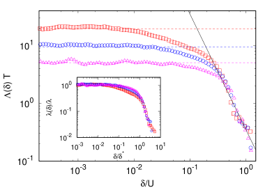
Figure 5: (Color online) Finite-size Lyapunov exponents $\Lambda(\delta)$ (FSLE) as a function of the velocity uncertainty $\delta$ for $N=1024$ (red squares) $N=512$ (blue circles) $N=256$ (purple triangles). The values of the Lyapunov exponents $\lambda$ are also shown (dashed lines). Black solid line represents the scaling $\Lambda(\delta)\sim\delta^{-2}$. Inset: The FSLE $\Lambda(\delta)$ rescaled by the Lyapunov exponents $\lambda$ as a function of the rescaled uncertainty $\delta/\delta^{*}$.

In conclusion, we studied the chaotic and predictability properties of fully developed turbulence by simulating two realizations of the velocity field initially separated by a very small perturbation. At short times the separation increases exponentially as a consequence of the chaoticity of the flow. Finite perturbations increase linearly in time, as predicted by dimensional arguments, and the time for the perturbation to affect a wavenumber $k$ in the inertial range is proportional to $\varepsilon^{-1/3}k^{-2/3}$.

The Lyapunov exponent is found to grow with the Reynolds number faster than what predicted by a dimensional argument and intermittency models and, as a consequence, the product $\lambda\tau_{\eta}$ grows with $Re$. This indicates that the strong, intermittent fluctuations of turbulence at small scales give diverse contributions on different observables. In addition to the interest for many applications, turbulence is a prototypical example of system with many scales and characteristic times. Our results on the chaoticity of turbulence and its dependence on the number of active degrees of freedom are therefore of general interest for the study of extended dynamical systems.