On Fermat curves modulo a finite number

Abstract.

We show that the existence of a non-trivial solution of $x^{n}+y^{n}=p^{n}$, with $p$ a prime number, is equivalent to the existence of a solution of a certain (over-determined) system of $(n-1)$-recursion relations (”zipper” equations) in $\mathbb{Z}_{p-1}$.

1. Introduction

The famous Fermat’s last theorem states that the equation $x^{n}+y^{n}=z^{n}$ admits no positive integral solutions, if $n\geq 3$, see [1, 2] and references therein. But what happens if we ease the condition and require for points $(x,y)\in\mathbb{Z}^{2}$ for which $z^{n}$ just divides $x^{n}+y^{n}$, for some fixed $z\in\mathbb{Z}$? In general, this leads us to define the main subject of study in this work:

Definition: For $n\in\mathbb{N}$ and $j\geq 1$ let

$$T_{n}(z;j):=\left\{(x,y)|x^{n}+y^{n}\equiv 0\textrm{ (mod }z^{j})\right\}\subset(\mathbb{Z}_{z^{j}})^{2}$$

be the $j$-th Fermat tile of radius $z$.

We think of elements of $T_{n}(z;n)$ as ”mock solutions” of the equation $x^{n}+y^{n}=z^{n}$ (as clearly, a genuine solution, if exists, induces an element of $T_{n}(z;n)$ but not the other way around). Remarkably, not only do such ”mock solutions” exist, they actually satisfy a neat algebraic structure which we describe, using Fermat’s little theorem, in section 2. From the elementary features of the plane geometry of Fermat curves, it follows that the tiles $T_{n}(z;n)$ satisfy the following property:

Proposition A: If $(x,y,z)\in\mathbb{Z}_{+}^{3}$ is a solution of $x^{n}+y^{n}=z^{n}$ then $(x,y)\in T_{n}(z;n)\cap[0,z]^{2}$.

In section 3 we study the properties of elements $(x,y)\in T_{n}(p;n)\cap[0,p]^{2}$, for $p$ a prime number, and show that such elements are subject to a substantial system of highly non-trivial restrictions. The description of these restrictions requires a study of the functions

$$\begin{array}[]{ccc}Log_{j}:\mathbb{Z}^{\ast}_{p^{j}}\rightarrow\mathbb{Z}_{\phi(p^{j})}&;&Exp_{j}:\mathbb{Z}_{\phi(p^{j})}\rightarrow\mathbb{Z}_{p^{j}}^{\ast}\end{array}$$

given by

$$\begin{array}[]{ccc}Log_{j}(g^{s})=[s]_{\phi(p^{j})}\in\mathbb{Z}_{\phi(p^{j})}&;&Exp_{j}(s):=[g^{s}]_{p^{j}}\in\mathbb{Z}_{p^{j}}\end{array},$$

where $\phi(p^{j})=(p-1)\cdot p^{j-1}$ is the totinet function and $j\geq 1$. The main feature is the definition of a natural class of functions of the form $A^{a}_{j}:\mathbb{Z}_{p-1}\times\mathbb{Z}_{p^{j-1}}\rightarrow\mathbb{Z}_{p}$, for $a\in\mathbb{Z}_{p-1}$. In terms of these functions, the restrictions are given as follows:

Theorem B (”zipper” relations): If $(x,y)\in T_{n}(p;n)\cap[0,p]^{2}$ there exists an element $s=s_{(x,y)}\in\mathbb{Z}_{p-1}$ and $a\in\mathbb{Z}_{p-1}$ which satisfy the following overdetermined double recursion (”zipper”) relations

$$\left\{\begin{array}[]{c}r_{0}=A^{0}_{1}(s)=A^{a}_{1}(s)\\ r_{1}=A^{0}_{2}(s;r_{0})=A^{a}_{2}(s;r_{0})\\ \vdots\\ r_{n-1}=A_{n}^{0}(s;r_{0}...,r_{n-2})=A_{n}^{a}(s;r_{0}...,r_{n-2})\end{array}\right.$$

As one can see the number of equations in the variable $s\in\mathbb{Z}_{p-1}$ grows with $n$ (in the Pythagorean case $n=2$, there is one equation). In particular, Fermat’s last theorem would follow from showing that the zipper relations have no solutions for $n\geq 3$. We define and study various properties of the zipper relations in section 4.

The rest of the work is organized as follows: In section 2 we describe Fermat tiles, in section 3 we study $Log_{j}$ and $Exp_{j}$ and define $A^{a}_{j}$. In section 4 we define the zipper relations.

2. The geometric structure of Fermat tiles

Before describing Fermat tiles in general, let us start with a few examples (which justify the term tile).

Example 2.1 (n = 2): Figure 4 shows the first Fermat tile $T_{2}(5,1)$ of radius $5$.

Figure 1. First Fermat tile $T_{2}(5,1)$ of radius $5$.

Figure 5 shows the second Fermat tile $T_{2}(5,2)$ of radius $5$.

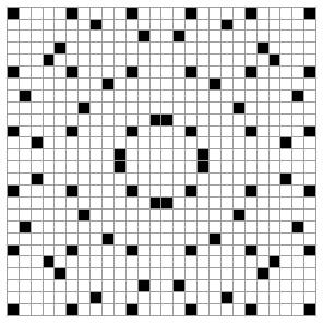
Figure 2. Second Fermat tile $T_{2}(5,2)$ of radius $5$.

Note that, as expected, one has $(3,4),(4,3),(5,0),(0,5)\in T_{2}(5,2)\cap[0,5]^{2}$.

Example 2.2 ($n\geq 3$): Figure 6 shows the first Fermat tile $T_{4}(7,1)$ of radius $7$:

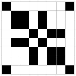
Figure 3. Second Fermat tile $T_{3}(7,1)$ of radius $7$.

Figure 7 shows the first Fermat tile $T_{4}(17,1)$ of radius $17$

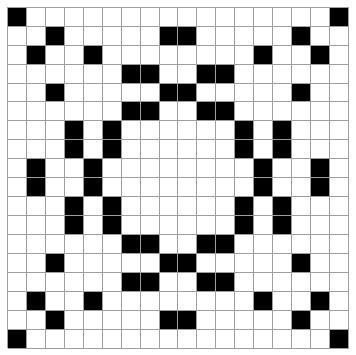
Figure 4. First Fermat tile $T_{4}(17,1)$ of radius $17$.

We refer to

$$C_{n}(z):=\left\{(x,y)|x^{n}+y^{n}=z^{n}\right\}\subset\mathbb{R}^{2}$$

as the $n$-th Fermat curve of radius $z\in\mathbb{R}$. Note that Fermat’s last theorem is equivalent to stating that $C_{n}(z)\cap\mathbb{N}^{2}=\left\{(z,0),(0,z)\right\}$ for any $n\geq 3$ and $z\in\mathbb{N}$. Let us proceed with the following remark:

Remark 2.3 (plane geometry of Fermat curves): Figure 5 shows $C_{2}(5)$, the circle of radius $z=5$, with the integer lattice:

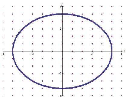
Figure 5. Graph of $C_{2}(5)$ together with the integer lattice $\mathbb{Z}^{2}$.

Recall that a solution $(x,y,z)\in\mathbb{N}^{3}$ of $x^{2}+y^{2}=z^{2}$ is called a Pythagorean triple. Note that $C_{2}(5)\cap\mathbb{N}^{2}=\left\{(3,4),(4,3),(5,0),(0,5)\right\}$. Figure 6 shows $C_{8}(5)$ with the integral lattice

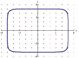
Figure 6. Graph of $C_{8}(5)$ together with the integer lattice $\mathbb{Z}^{2}$.

Figure 7 shows $C_{9}(10)$ with the integer lattice

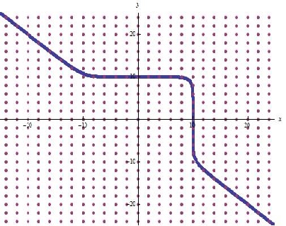
Figure 7. Graph of $C_{9}(10)$ together with the integer lattice $\mathbb{Z}^{2}$.

In particular, it is easy to see that Fermat curves satisfy $C_{n}(z)\cap(\mathbb{R}^{+})^{2}\subset[0,z]^{2}$ for any $n\in\mathbb{N}$ and $z\in\mathbb{R}^{+}$.

Note that, in view the above remark, showing that

$$T_{n}(z;n)\cap[0,z]^{2}=\left\{(0,0),(z,0),(0,z),(z,z)\right\}$$

would imply Fermat’s last theorem. Let us now turn to describe the structure of the $j$-th Fermat tile, $T_{n}(p,j)$, for $p$ a prime number. Let us start with the following:

Lemma 2.4: Let $S_{n}(p)\subset\mathbb{Z}_{p}$ be the solution set of the equation $x^{n}+1\equiv 0\textrm{ (mod }p)$ and let $g\in\mathbb{Z}_{p}$ be a primitive generator.

(a) If $2n\mid(p-1)$ then $S_{n}(p)=\left\{g^{a_{0}+im}\right\}_{i=0}^{n-1}$ where $a_{0}:=\frac{p-1}{2n}$ and $m:=\frac{p-1}{n}$.

(b) If $2n\nmid(p-1)$ then $S_{n}(p)=\emptyset$.

Proof: As $g\in Z_{p}$ is a primitive generator we have

$$\left\{g^{s}|s=0,...,p-2\right\}\subset\mathbb{Z}^{\ast}_{p}$$

By Fermat’s little theorem $g^{\frac{p-1}{2}}\equiv-1\textrm{ (mod }p)$. Hence, we are looking for some $x=g^{a}$ such that

$$g^{n\cdot a}\equiv g^{\frac{p-1}{2}}\textrm{ (mod }p).$$

Again, by Fermat’s little theorem, this is equivalent to solving

$$n\cdot a\equiv\frac{p-1}{2}\textrm{ (mod }p-1).$$

The solutions are given by $a_{i}:=a_{0}+im$ for $i=0,..,n-1$. $\hskip 142.26378pt\square$

Consider the following example:

Example 2.5: Let $n=4$ and $p=17$. One has $a_{0}=2,m=4$ and $g=3$. Hence

$$S_{4}(17)=\left\{3^{2},3^{6},3^{10},3^{14}\right\}=\left\{9,15,8,2\right\}\subset\mathbb{Z}_{17},$$

which coincides with the first row of Fig. 4, as expected.

We have:

Proposition 2.6 (reducibility): For any $1\leq j\leq n$ the following holds:

(a) If $2n\mid(p-1)$ then $T_{n}(p,j)=\left\{\left(a,ax^{p^{j-1}}\right)|x\in S_{n}(p),a\in\mathbb{Z}_{p^{j}}\right\}\cup\left(p\mathbb{Z}_{p^{j-1}}\right)^{2}$.

(b) If $2n\nmid(p-1)$ then $T_{n}(p,j)=\left(p\mathbb{Z}_{p^{j-1}}\right)^{2}$.

For $x\in S_{n}(p),j\in\mathbb{N}$ consider the linear function $f^{j}_{x}:\mathbb{Z}_{p^{j}}\rightarrow\mathbb{Z}_{p^{j}}$ given by $a\mapsto ax^{p^{j-1}}$. Set

$$T(x;j):=graph(f^{j}_{x})=\left\{\left(a,ax^{p^{j-1}}\right)|a\in\mathbb{Z}_{p^{j}}\right\}.$$

Consider the following example:

Example 2.7: Let $n=4$ and $p=17$. Figure 8 shows the graphs of $f^{1}_{x}:\mathbb{Z}_{17}\rightarrow\mathbb{Z}_{17}$ for $x=9,15,8,2$

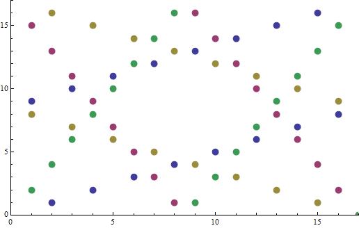
Figure 8. Graphs of $f^{1}_{x}$ for $x=9,15,8,2$.

As one can see, Figure 8 coincides with the interior of the Fermat tile $T_{4}(17,1)$, presented in Figure 7. Figure 9 presents the four linear components separately:

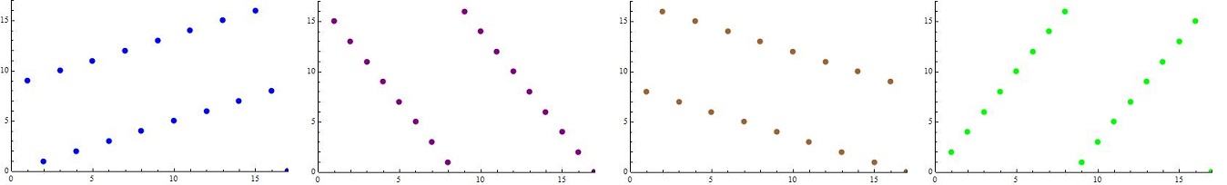
Figure 9. Separated graphs of $f^{1}_{x}$ for $x=9,15,8,2$.

Figure 10 shows the graphs of $f^{2}_{x}:\mathbb{Z}_{17^{2}}\rightarrow\mathbb{Z}_{17^{2}}$ for $x=9,15,8,2$

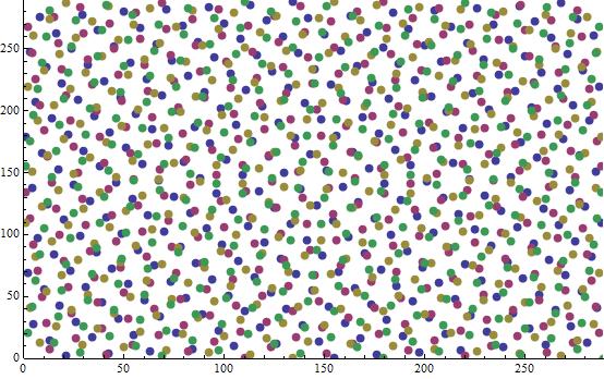
Figure 10. Graphs of $f^{2}_{x}$ for $x=9,15,8,2$.

Figure 11 presents the four linear components separately:

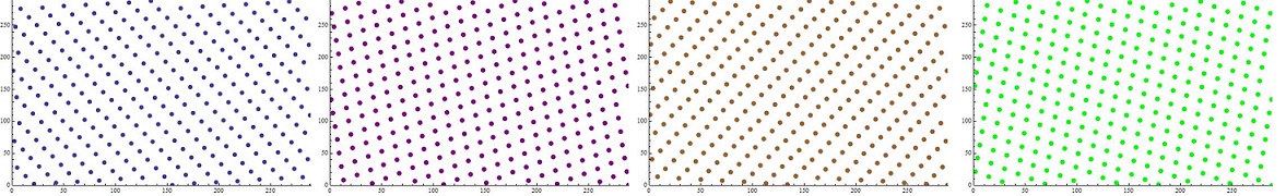
Figure 11. Separated graphs of $f^{2}_{x}$ for $x=9,15,8,2$.

In view of the above, Fermat’s last theorem would thus follow from showing

$$T(x;n)\cap[0,p]^{2}=\left\{(0,0)\right\}\hskip 14.22636pt\textrm{ for all }\hskip 7.11317ptx\in S_{n}(p).$$

That is, showing $f_{x}^{n}(a)>p$ for any $1\leq a\leq p$ . First, let us make the following remark:

Remark 2.8 (empirics): $T(x;j)$, is the graph of a line of slope $x^{p^{j-1}}$ in $\mathbb{Z}^{2}_{p^{j}}$, for $x\in S_{n}(p)$. In parctice, such a line actually traces a $2$-dimensional lattice in $\mathbb{Z}_{p^{j}}^{2}$, due to the truncation caused by the quotient relation (see Fig. 11 and 13). Empirics show that, for various values of $j$ and $x$, typically, the values of $T(x;j)$ can be bounded by a line $a_{2}=\frac{m_{j}(x)\cdot a_{1}}{n_{j}(x)}+\frac{p^{j}}{n_{j}(x)}$ with $m_{j}(x)<\sqrt{p}^{j}$. Figure 12 shows $(a,f^{3}_{x}(a))$ for $9\in S_{4}(17)$ in $[0,p^{2}]\times[0,p^{3}]$ and $[0,p^{2}]\times[0,p^{2}]$, together with the bounding line $a_{2}=-\frac{23}{47}\cdot a_{1}+\frac{17^{3}}{47}$:

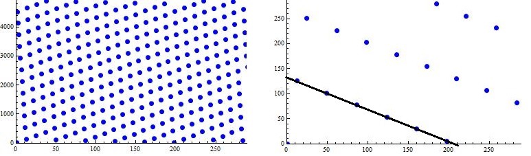
Figure 12. $(a,f^{3}_{x}(a))$ in $[0,17^{2}]\times[0,17^{3}]$ and $[0,17^{2}]\times[0,17^{2}]$.

Note that, if such a line exists in general, for $j\geq 3$, it would need to go more than $p$ steps in the $a_{1}$-axis to go below $p$ in the $a_{2}$-axis and, in particular, $f^{j}_{x}(a)>p$ if $0\leq a\leq p$. However, showing that such a line exists, in general, requires for a more solid understanding of $T(x;j)\subset\mathbb{Z}_{p^{j}}^{2}$ (the subject of the following section).

It is also interesting to note the following: set $x_{i}=g^{a_{i}}\in S_{n}(p)$ for $i=0,...,n-1$ and denote $\theta_{i}^{j}(p,n)$ be the number of elements $0\leq a\leq p$ such that $f^{j}_{x_{i}}(a)<p$ (we want $\theta^{n}_{i}(p,n)=0$ for all $i$). For $n=4$ we actually have

$$\tiny\left(\begin{array}[]{ccccccccccccccccccccc}p&17&41&73&89&97&113&137&193&233&241&257&281&313&337&353&401\\ \theta^{2}_{1}&1&3&2&0&3&0&1&2&1&0&1&1&1&1&1&0\\ \theta^{2}_{2}&1&0&0&1&0&1&0&0&0&1&1&0&1&1&1&3\\ \theta^{2}_{3}&1&0&0&1&0&1&0&0&0&1&1&0&1&1&1&3\\ \theta^{2}_{4}&1&3&2&0&3&0&1&2&1&0&1&1&1&1&1&0\\ \sum\theta_{i}^{3}&0&0&0&0&0&0&0&0&0&0&0&0&0&0&0&0\end{array}\right).$$

3. Some remarks on the arithemetics of the ring of invertibles $\mathbb{Z}^{\ast}_{p^{j}}$

Let $g\in\mathbb{Z}_{p}$ be a fixed primitive generator. It is easy to see that $g$ is a primitive generator for $\mathbb{Z}_{p^{j}}$ for all $j\geq 1$, as well. Recall that the ring of invertibles is given by

$$\mathbb{Z}^{\ast}_{p^{j}}=\left\{a|a\not\equiv 0\textrm{ (mod }p)\right\}\subset\mathbb{Z}_{p^{j}}.$$

Set $\phi(p^{j}):=(p-1)\cdot p^{j-1}$. Let us consider the following two functions

$$\begin{array}[]{ccc}Log_{j}:\mathbb{Z}^{\ast}_{p^{j}}\rightarrow\mathbb{Z}_{\phi(p^{j})}&;&Exp_{j}:\mathbb{Z}_{\phi(p^{j})}\rightarrow\mathbb{Z}_{p^{j}}^{\ast}\end{array}$$

given by $Log_{j}(g^{s})=[s]_{\phi(p^{j})}\in\mathbb{Z}_{\phi(p^{j})}$ and $Exp_{j}(s):=[g^{s}]_{p^{j}}\in\mathbb{Z}_{p^{j}}$. By definition, the amobea corresponding to the linear tile $T(x;j)$ is simply given by the following affine line

$$\mathcal{A}(x_{i};j):=Log_{j}\left(T(x_{i};j)\cap(\mathbb{Z}_{p^{j}}^{\ast})^{2}\right)=\left\{(s_{1},s_{2})|s_{1}-s_{2}=a_{i}\cdot p^{j-1}\right\}\subset\mathbb{Z}^{2}_{\varphi(p^{j})},$$

where $Log_{1}(x_{i})=a_{i}=\frac{(1+2i)\cdot(p-1)}{2n}$, with $i=0,...,n-1$. In particular, we want to show

$$max\left\{Exp_{n}(s),Exp_{n}(s+a_{i}\cdot p^{n-1})\right\}\geq p,$$

for any $s\in\mathbb{Z}_{\phi(p^{n})}$ and $i=0,...,n-1$.

Remark 3.1 (Transcendentality of $Log_{j}$ and $Exp_{j}$): It should be noted that finding a general full explicit description of $Log_{j}$ and $Exp_{j}$ is considered a completely transcendental question. For instance, Fig. 13 is a graph of $Log_{1}(a)\in\mathbb{Z}_{96}$ for $a\in\mathbb{Z}_{97}$ with $g=5$:

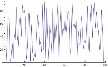
Figure 13. $Log_{1}(a)$ for $p=97$ and $g=5$.

Note that, by definition, $[Exp_{j+1}(s)]_{p^{j}}=Exp_{j}([s]_{\phi(p^{j})})$. Hence, for any $j\geq 1$ we can define the function $g_{j}:\mathbb{Z}_{\varphi(p^{j+1})}\rightarrow\mathbb{Z}_{p}$ given by

$$g_{j}(s):=\frac{Exp_{j+1}(s)-Exp_{j}([s]_{\phi(p^{j})})}{p^{j}}.$$

Consider the formal series

$$Exp(s,T):=Exp_{1}([s]_{p-1})+\sum_{i=1}^{\infty}g_{j}([s]_{\phi(p^{j+1})})\cdot T^{j}.$$

The formal series satisfies $Exp_{j}(s)=[Exp(s,p)]_{p^{j}}$. In particular, note that

$$\left\{\begin{array}[]{c}Exp_{j}(s)\leq p\Leftrightarrow g_{1}(s)=...=g_{j-1}(s)=0,\\ Exp_{j}(s+a\cdot p^{j-1})\leq p\Leftrightarrow g_{1}(s+a\cdot p)=...=g_{j-1}(s+a\cdot p^{j-1})=0\end{array}\right.$$

Note that an element $r\in\mathbb{Z}_{p^{j}}$ can be uniquely expressed as

$$r=r_{0}+r_{1}\cdot p+...+r_{j-1}\cdot p^{j-1},$$

such that $r_{i}\in\mathbb{Z}_{p}$ for any $1\leq i\leq j-1$. For $a\in\mathbb{Z}_{p-1}$, let $h^{a}_{j}:\mathbb{Z}_{p-1}\times\mathbb{Z}_{p^{j}}\rightarrow\mathbb{Z}_{p}$ be the function given by

$$h_{j}^{a}(s;r_{0},...,r_{j-1}):=g_{j}\left(s,r_{0}+r_{1}\cdot p+...+r_{j-1}\cdot p^{j-1}+a\cdot p^{j}\right).$$

It is easy to see that:

Lemma 3.2 (shift): For any $a\in\mathbb{Z}_{p-1}$ and $j\geq 1$ the following holds

$$h_{j}^{a}(s;r_{0},...,r_{j-1})=h^{0}_{j}(s+a;r_{0}+a+r(s+a),...,r_{j-1}+a+r(s+a)),$$

where $r(m)=\frac{(m-[m]_{p-1})}{p-1}$.

For instance, consider the following example:

Example 3.3 ($p=5$ and $j=1$): The following is a table of the values of $h^{0}_{1}(s,r)$ for $p=5$

$$\left(h^{0}_{1}(s,r)\right)_{0,0}^{3,4}=\left(\begin{array}[]{ccccc}0&3&1&4&2\\ 0&1&2&3&4\\ 0&2&4&1&3\\ 1&0&4&3&2\end{array}\right).$$

The values of $h^{3}_{1}(s_{1},s_{2})$ are given by

$$\left(h^{3}_{1}(s,r)\right)_{0,0}^{3,4}=\left(\begin{array}[]{cccccc}3&2&1&0&4\\ 2&0&3&1&4\\ 4&0&1&2&3\\ 3&0&2&4&1\end{array}\right)$$

Note that $(s^{0},r^{0})=(3,1)$ is a point satisfying $h_{1}^{0}(s^{0},r^{0})=h_{1}^{3}(s^{0},r^{0})=0$. Indeed,

$$\begin{array}[]{ccc}Exp_{2}(7)=Exp_{2}(3+1\cdot 4)=3&;&Exp_{2}(2)=Exp_{2}([22]_{20})=Exp_{2}(7+3\cdot 5)=4\end{array},$$

which represents the Pythagorean point $(3,4)\in C_{2}(5)$, as expected.

In general, for any $j\geq 1$, set

$$Z_{j}(a):=\left\{(s,r)|h_{k}^{a}(s,r_{0},...,r_{k-1})=0\textrm{ for any }k\leq j\right\}\subset\mathbb{Z}_{p-1}\times\mathbb{Z}_{p^{j}}.$$

Let $p$ be a prime and $2\leq n\in\mathbb{N}$ an integer such that $2n/(p-1)$. Set $a_{i}:=\frac{(1+2i)(p-1)}{2n}$ for $i=1,...,n-1$. Our main object of study now is $Z_{n-1}(0)\cap Z_{n-1}(a_{i})$. In particular, note that according to the above, showing

$$Z_{n-1}(0)\cap Z_{n-1}(a_{i})=\emptyset$$

would imply Fermat’s last theorem. Consider, for instance, the following example:

Example 3.4 ($p=5$ and $j=2$): Note from the previous example that, for $(s,r_{0})=(3,1)$, we have

$$h^{0}_{1}(3;1)=h^{3}_{1}(3;1)=h^{0}_{1}(6;4)=h^{0}_{1}(1,0)=0.$$

Note also that

$$\begin{array}[]{ccc}h_{1}^{0}(3,r)=[4\cdot(r-1)]_{5}&;&h_{1}^{0}(2,r)=[2\cdot r]_{5}\end{array}.$$

For $j=2$, we have

$$\left(h_{2}^{0}\left(3;r_{0},r_{1}\right)\right)_{0,0}^{4,4}=\left(\begin{array}[]{ccccc}0&4&3&2&1\\ 0&4&3&2&1\\ 1&0&4&3&2\\ 0&4&3&2&1\\ 1&0&4&3&2\end{array}\right),$$

and

$$\left(h_{2}^{0}\left(2;r_{0},r_{1}\right)\right)_{0,0}^{4,4}=\left(\begin{array}[]{ccccc}0&2&4&1&3\\ 2&4&1&3&0\\ 0&2&4&1&3\\ 0&2&4&1&3\\ 0&2&4&1&3\end{array}\right).$$

As one can see, we can still express

$$\begin{array}[]{ccc}h_{2}^{0}(3,r_{0},r_{1})=[4\cdot(r_{1}-A^{0}_{2}(3;r_{0}))]_{5}&;&h_{2}^{0}(2,r_{0},r_{1})=[2\cdot(r_{1}-A^{0}_{2}(2;r_{0}))]_{5}\end{array},$$

where $A^{0}_{2}:\mathbb{Z}_{p-1}\times\mathbb{Z}_{p}\rightarrow\mathbb{Z}_{p}$ is a non-linear function, determining the position of the zero in the $r_{0}$-row (see Lemma 3.5 below). In particular, note that the linear system

$$\begin{array}[]{ccc}h^{0}_{2}(3;1,r_{1})=[4\cdot r_{1}]_{5}=0&;&h^{0}_{2}(2;1,r_{1})=[2\cdot(r_{1}-4)]_{5}=0\end{array}$$

has no solution. Hence $Z_{1}(0)\cap Z_{1}(3)=\left\{(3,1)\right\}$ while $Z_{2}(0)\cap Z_{2}(3)=\emptyset$. Finally, it should be noted that the values of $Exp_{1}(s)$ for $s\in\mathbb{Z}_{4}$ are given by

$$\left(\begin{array}[]{ ccccc}s&0&1&2&3\\ Exp_{1}(s)&1&2&4&3\end{array}\right).$$

In particular, $h_{2}^{0}$ can be expressed in the following form

$$h_{2}^{0}(s;r_{0},r_{1})=[Exp_{1}([s+3]_{4})\cdot(r_{1}-A^{0}_{2}(s;r_{0}))]_{5}.$$

In general, we have:

Lemma 3.5: For any $a\in\mathbb{Z}_{p-1}$ and $j\geq 1$ there exists $A^{a}_{j}:\mathbb{Z}_{p-1}\times\mathbb{Z}_{p^{j-1}}\rightarrow\mathbb{Z}_{p}$ and $s_{0}\in\mathbb{Z}_{p-1}$, such that

$$h^{a}_{j}(s;r_{0},...,r_{j-1})=[Exp_{1}(s+a+s_{0})\cdot(r_{j-1}-A_{j}^{a}(s;r_{0},..,r_{j-2}))]_{p}.$$

First, note that, due to the shift property

$$A_{j}^{a}(s;r_{0},...,r_{j-2})=A_{j}^{0}(s+a;r_{0}+a+r(s+a);...;r_{j-2}+a+r(s+a))-(a+r(s+a)).$$

For instance, consider the following example:

Example 3.6: For $p=5$ and $j=1$ we have

$$\left(\begin{array}[]{ccccc}s&0&1&2&3\\ A_{1}^{0}&0&0&0&1\\ A_{1}^{3}&3&1&1&1\end{array}\right).$$

Indeed, note that

$$\begin{array}[]{ccc}A^{3}_{1}(0)=[A_{1}^{0}(3)-3]_{5}=[1-3]_{5}=[-2]=3&;&A^{3}_{1}(1)=[A^{0}_{1}(4)-(3+r(1+3))]_{5}=[-4]_{5}=1\end{array}.$$

The study of various properties of the functions $A^{a}_{j}$, defined in Lemma 3.5, is the subject of the next section.

4. The double recursion (”zipper”) equations

For any $1\leq k\leq j$, set

$$Z^{k}_{j}(a):=\left\{(s,r)|h_{k}^{a}(s,r_{0},...,r_{k-1})=0\right\}\subset\mathbb{Z}_{p-1}\times\mathbb{Z}_{p^{j}}.$$

Note that

$$Z_{j}(a)=Z_{j}^{1}(a)\cap...\cap Z_{j}^{j}(a).$$

By definition,

$$Z_{j}^{k}(a)=\left\{(s,r_{0},...,r_{k-2},A_{k}^{a}(s;r_{0},...,r_{k-2}),r_{k},...,r_{j-1})\right\}\subset\mathbb{Z}_{p-1}\times\mathbb{Z}_{p^{j}}.$$

Hence, from the above description, we deduce that $(s;r_{0},...,r_{j-1})\in Z_{j}(a)$ if and only if it is a solution of the following recursion relations

$$\begin{array}[]{ccccccc}r_{0}=A^{a}_{1}(s)&;&r_{1}=A^{a}_{2}(s;r_{0})&;&...&;&r_{j-1}=A_{j}^{a}(s;r_{0}...,r_{j-2})\end{array}$$

In conclusion, combining the above relations for $Z_{j}(0)$ and $Z_{j}(a)$, we get:

Theorem 4.1 (”zipper” relations): Let $j\geq 1$. Then $(s;r_{0},...,r_{j-1})\in Z_{j}(0)\cap Z_{j}(a)$ if and only if it is a solution of the following (overdetermined) double recursion relations

$$\left\{\begin{array}[]{c}r_{0}=A^{0}_{1}(s)=A^{a}_{1}(s)\\ r_{1}=A^{0}_{2}(s;r_{0})=A^{a}_{2}(s;r_{0})\\ \vdots\\ r_{j}=A_{j+1}^{0}(s;r_{0}...,r_{j-1})=A_{j+1}^{a}(s;r_{0}...,r_{j-1})\end{array}\right.$$

As mentioned in section 3, showing that the zipper relations admit no solutions for $j=n-1$ would imply Fermat’s last theorem. Let us conclude this section with a few further remarks on the properties of the zipper relations.

Remark 4.2 (the geometry of $A^{a}_{j}$): The zipper relations are given in terms of the functions $A^{a}_{j}(s;r_{0},...,r_{j-2})$ which, by definition, represent a parametrization of the zero set of the function $h^{a}_{j}(s;r_{0},...,r_{j-1})$. It is interesting to note that the dependency of $A^{a}_{j}$ on the $s$-parameter is essentially different than its dependency on the $r=(r_{0},...,r_{j-2})$ parameters. For instance, let $p=97$, $n=4$ and $a=(96/8)=12$. Figure 14 shows a matrix-plot of the function $h^{a}_{2}(s_{0};r_{0},r_{1})$ for $s_{0}=Log_{1}(11)$ fixed.

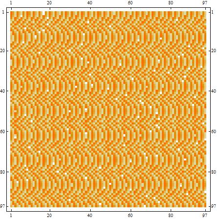
Figure 14. Matrix-plot for $h^{a}_{2}(s;r_{0},r_{1})$ for $(r_{0},r_{1})\in\mathbb{Z}_{p}^{2}$.

In particular, it might seem that the zeros of $h_{j}^{0}(s;r_{0},r_{1})$ (white points) are randomly distributed in the $r$-coordinates. However, they are determined as the local minima of a one-parametric family of quadrics dominating the picture. Hopefully, we would give a more detailed description of this one parametric family of quadrics in a future work.

On the other hand, it seems that, in the $s$-coordinate, the function $A^{a}_{j}(s;r)$ inherits the chaotic behavior of $Log_{1}(s)$. For instance, Figure 15 is a graph of $A_{1}^{a}(s)$ for the same parameters as above:

Figure 15. $A^{a}_{1}(s)$ for $s\in\mathbb{Z}_{96}$ with $a=12$.

Furthermore, it is also interesting to note, for the above parameters, that the solutions of the first zipper equation are give by

$$\left\{s|A^{0}_{1}(s)=A^{a}_{1}(s)\right\}=\left\{Log_{1}(11),Log_{1}(22),Log_{1}(33)\right\}\subset\mathbb{Z}_{96}.$$

On the other hand, the second zipper equations for these elements are already non-zero

$$\left(A_{2}^{0}(Log_{1}(11),A^{0}_{1}(Log_{1}(11))-A_{2}^{a}(Log_{1}(11),A^{0}_{1}(Log_{1}(11))\right)=$$

$$=\left(A_{2}^{0}(Log_{1}(22),A^{0}_{1}(Log_{1}(22))-A_{2}^{a}(Log_{1}(22),A^{0}_{1}(Log_{1}(22))\right)=$$

$$=\left(A_{2}^{0}(Log_{1}(33),A^{0}_{1}(Log_{1}(33))-A_{2}^{a}(Log_{1}(33),A^{0}_{1}(Log_{1}(33))\right)=3\neq 0.$$

Moreover, note that the value of the second zipper equation is actually independent of the element of the solution set of $A^{a}_{1}(s)=A^{0}_{1}(s)$ chosen. This repeats itself in other cases as well.

The above remark shows that $A^{a}_{j}(s,r)$ seems to be chaotic in the $s$-parameter and non-linear in the $r$-parameter. In order to overcome this, let us note that if $(s;A^{0}_{1}(s),A^{0}_{2}(s;A_{1}^{0}(s)))$ is a solution, for instance, of the first two zipper equations it needs to satisfy

$$\begin{array}[]{ccc}h_{1}^{a}\left(s;A^{0}_{1}(s)\right)=0&;&h_{1}^{0}\left(s;A^{a}_{1}(s)\right)=0\\ h_{2}^{a}\left(s;A^{0}_{1}(s),A^{0}_{2}(s;A_{1}^{0}(s))\right)=0&;&h_{2}^{0}\left(s;A^{a}_{1}(s),A^{a}_{2}(s;A_{1}^{a}(s))\right)=0\end{array}.$$

In view of this, let us define for $i=1,2$ the functions $H^{0}_{i},H^{a}_{i}:\mathbb{Z}_{p-1}\rightarrow\mathbb{Z}_{p}$ given by

$$\begin{array}[]{ccc}H_{1}^{a}(s):=h_{1}^{a}\left(s;A^{0}_{1}(s)\right)&;&H_{1}^{0}(s):=h_{1}^{0}\left(s;A^{a}_{1}(s)\right)\\ H^{a}_{2}(s):=h_{2}^{a}\left(s;A^{0}_{1}(s),A^{0}_{2}(s;A_{1}^{0}(s))\right)&;&H^{0}_{2}(s):=h_{2}^{0}\left(s;A^{a}_{1}(s),A^{a}_{2}(s;A_{1}^{a}(s))\right)\end{array}.$$

Further define $\widetilde{H}^{0}_{i},\widetilde{H}^{a}_{i}:\mathbb{Z}_{p}^{\ast}\rightarrow\mathbb{Z}_{p}$ by $\widetilde{H}^{0}_{i}(t)=H^{0}_{i}(Log_{1}(t))$ and $\widetilde{H}^{a}_{i}(t)=H^{a}_{i}(Log_{1}(t))$. Remarkably, contrary to $A^{0}_{i}(s;r)$ which are chaotic as functions of $s$, the functions $\widetilde{H}^{0}_{i},\widetilde{H}^{a}_{i}$ are actually quite patterned. In fact, Figure 16 shows the graphs of $\widetilde{H}^{0}_{1},\widetilde{H}^{a}_{1}$ for $p=97$ and $a=12$:

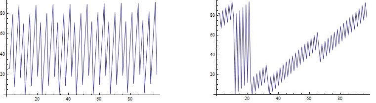
Figure 16. $\widetilde{H}^{0}_{1}(t)$ (left) and $\widetilde{H}^{a}_{1}(t)$ (right) for $t\in\mathbb{Z}^{\ast}_{97}$ with $a=12$.

Note that, as expected, $\widetilde{H}^{0}_{1}(t)=\widetilde{H}^{a}_{1}(t)=0$ for $t=11,22,33$. Figure 17 shows the graphs of $\widetilde{H}^{0}_{2}(t),\widetilde{H}^{a}_{2}(t)$:

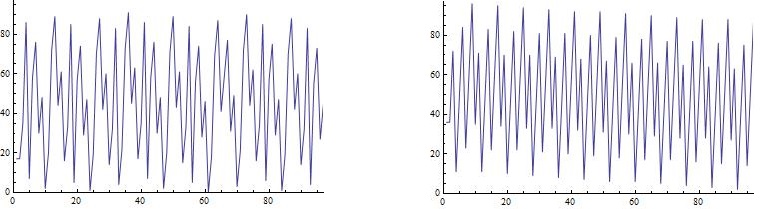
Figure 17. $\widetilde{H}^{0}_{2}(t)$ (left) and $\widetilde{H}^{a}_{2}(t)$ (right) for $t\in\mathbb{Z}^{\ast}_{97}$ with $a=12$.

As expected, one clearly sees that these four graphs have no common zero. In order to further describe $\widetilde{H}^{a}_{i}$ let us introduce their derivatives. Let $F:\mathbb{Z}_{p}^{\ast}\rightarrow\mathbb{Z}_{p}$ be a function. We refer to the function $D(F):\mathbb{Z}_{p}^{\ast}\rightarrow\mathbb{Z}_{p}$, given by $D(F)(t):=[f(t+1)-f(t)]_{p}$, as the derivative of $F$. For instance, Fig. 18 shows the derivatives $D(\widetilde{H}^{0}_{1})$ and $D(\widetilde{H}^{a}_{1})$:

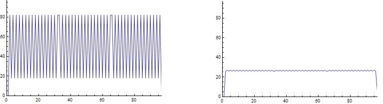
Figure 18. $D(\widetilde{H}^{0}_{1}(t))$ (left) and $D(\widetilde{H}^{a}_{1}(t))$ (right) for $t\in\mathbb{Z}^{\ast}_{97}$ with $a=12$.

Figure 19 shows the graphs of the derivatives $D(\widetilde{H}^{0}_{2})$ and $D(\widetilde{H}^{a}_{2})$:

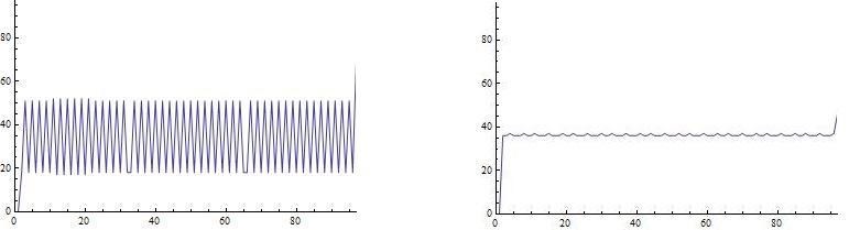
Figure 19. $D(\widetilde{H}^{0}_{2}(t))$ (left) and $D(\widetilde{H}^{a}_{2}(t))$ (right) for $t\in\mathbb{Z}^{\ast}_{97}$ with $a=12$.

What we see is that the functions $\widetilde{H}^{0}_{i},\widetilde{H}^{a}_{i}$ are semilinear, that is they have semi-constant first derivative. In particular, this derivative uniformly changes for $i=1,2$. It is now understandable to expect, that such a collection of four semi-linear curves in the plane $\mathbb{Z}_{p}^{2}$ cannot have a common solution. Showing this, in general, however, requires some further analysis.

References

[1] I. Kleiner.
From Fermat to Wiles: Fermat’s Last Theorem Becomes a Theorem.
Elem. Math. 55: 19–37, 2010.
[2] A. Wiles.
Modular elliptic curves and Fermat’s Last Theorem.
Annals of Mathematics. 142 (3), 443–551, 1995.