Rate constants for the formation of SiO by radiative association

Abstract

Accurate molecular data for the low-lying states of SiO are computed and used to calculate rate constants for radiative association of Si and O. Einstein A-coefficients are also calculated for transitions between all of the bound and quasi-bound levels for each molecular state. The radiative widths are used together with elastic tunneling widths to define effective radiative association rate constants which include both direct and indirect (inverse predissociation) formation processes. The indirect process is evaluated for two kinetic models which represent limiting cases for astrophysical environments. The first case scenario assumes an equilibrium distribution of quasi-bound states and would be applicable whenever collisional and/or radiative excitation mechanisms are able to maintain the population. The second case scenario assumes that no excitation mechanisms are available which corresponds to the limit of zero radiation temperature and zero atomic density. Rate constants for SiO formation in realistic astrophysical environments would presumably lie between these two limiting cases.

1 Introduction

The formation of dust in environments such as the inner winds of AGB stars (Cherchneff, 2006), the ejecta of novae (Rawlings & Williams, 1989), and the ejecta of supernovae (Lepp et al., 1990) depends on the production of molecules, either as precursors of dust grains or as competitors to dust production.

The formation of CO and SiO in such environments can be modeled using large networks of chemical reactions, which depend on the knowledge of rate constants for individual chemical reactions relating to the molecule species. For example, these models have been applied in explaining the observations of CO (Lepp et al., 1990; Gearhart et al., 1999) and SiO (Liu & Dalgarno, 1996) in the ejecta of Supernova 1987A, the inner winds of AGB stars (Willacy & Cherchneff, 1998), and the outer envelopes of carbon-rich (Cherchneff, 2012; Li et al., 2014) and oxygen-rich (Li et al., 2016) stars. In fact, the observation of SiO in carbon-rich stars suggests a shock-induced chemistry which dissociates CO freeing-up atomic oxygen to form SiO and other oxides (Cherchneff, 2012).

While in typical interstellar medium (ISM) environments, SiO is formed primarily by the exchange reaction

$$\rm Si+OH\rightarrow SiO+H,$$ (1)

the radiative association (RA) process may become competitive, particularly in hydrogen-deficient gas. For applications to various astrophysical environments, RA was studied for CO (Dalgarno et al., 1990; Franz et al., 2011; Antipov et al., 2013) and for SiO (Andreazza et al., 1995; Forrey et al., 2016).

The RA process for SiO formation is believed to be a key step in the subsequent formation of silicates and dust (Marassi et al., 2015). Therefore, it is of considerable interest to provide a comprehensive set of reliable rate constants for all contributions to the RA processes

$$\rm Si+O\rightarrow SiO+h\nu,$$ (2)

and

$$\rm Si\cdot\cdot\cdot O\rightarrow SiO+h\nu,$$ (3)

where $h\nu$ represents an emitted photon. Here, the Si$\cdot\cdot\cdot$O metastable state in (3) may be formed as an intermediate step in process (2) or by an independent process such as inverse predissociation.

In a recent publication (Forrey et al., 2016), here referred to as paper I, our group performed detailed quantum chemistry calculations to obtain potential energy curves (PEC’s) and transition dipole moments (TDM’s) for the low-lying molecular states of SiO. We then used the high quality molecular data for the $X^{1}\Sigma^{+}$ and $A^{1}\Pi$ states, and the TDM coupling the states, to obtain rate constants for RA of Si(${}^{3}P$) and O(${}^{3}P$) via approach on the $A^{1}\Pi$ molecular curve. We found that the rate constants were roughly a factor of ten smaller than those calculated earlier by Andreazza et al. (1995).

In the present work, we extend our initial calculations reported in Paper I to include SiO formation by RA via approach on the $E^{1}\Sigma^{+}$, $2^{1}\Pi$, $3^{1}\Pi$, and $D^{1}\Delta$ molecular states. In addition to computing the direct RA contribution (2) for each intermediate electronic state, we also calculate tunneling and radiative lifetimes for all of the quasi-bound vibrational states in order to provide estimates of the indirect resonant contribution (3) for different kinetic conditions.

In paper I, we showed that resonances may play an important role in enhancing the rate constants for the formation of SiO. With the assumption that all quasi-bound levels were in local thermodynamic equilibrium (LTE), we obtained rate constants for low temperatures which were several orders of magnitude larger than those predicted by standard quantum scattering formulations. The RA rate constants were defined to include both direct and indirect (inverse predissociation) formation processes. The direct contribution was computed using semiclassical (Bates, 1951) and quantum mechanical methods (Zygelman & Dalgarno, 1990; Stancil et al., 1993; Nyman et al., 2015; Öström et al., 2016; Forrey et al., 2016) and excellent agreement was achieved. The indirect contribution relied on the kinetic LTE assumption for the quasi-bound levels, which would be applicable whenever collisional and/or radiative excitation mechanisms are able to maintain an equilibrium population. For low density environments which are not subjected to substantial radiation, the indirect contribution would clearly be less than the LTE result.

We now consider two rate constants which we believe represent limiting cases for RA. The first rate constant is the LTE rate constant described above. The second rate constant, referred to as the NLTE rate constant in the zero-density limit (ZDL), considers the indirect formation process for a non-LTE environment which has zero radiation temperature and an atomic density $n<<n_{cr},$ where $n_{cr}$ is the critical density determined by equating the efficiency of RA with that of three-body recombination (TBR). With this definition, the NLTE-ZDL rate constant is equivalent to conventional methods that include radiative broadening in the resonance contribution when the tunneling width is smaller than or comparable to the radiative width (Öström et al., 2016; Antipov et al., 2013; Bain & Bardsley, 1972; Bennett et al., 2003; Mrugala et al., 2003). For astrophysical environments with varying amounts of radiation and mass densities, the exact phenomenological RA rate constant would be expected to lie somewhere in-between the LTE and NLTE-ZDL rate constants reported here.

In addition to presenting two rate constants for each electronic potential curve, we also present two methods for computing the rate constants. Both methods utilize the Sturmian approach described previously (Forrey, 2013, 2015). The first method calculates the rate constant using an analytic evaluation of the thermal average with respect to the Maxwell velocity distribution. The second method calculates the cross section and performs the thermal average using numerical integration. This method is similar to conventional grid-based approaches for solving the Schrödinger equation, e.g. Numerov propagation (Cooley, 1961; Johnson, 1977). Grid-based methods generally need to be performed on a fine energy mesh in order to fully resolve the resonant contributions. In the present case (Method 2), the size of the Sturmian basis set determines the energy density of the numerical integration grid. The contributions from narrow resonances are well-resolved due to the variational nature of diagonalizing the Hamiltonian on an ${\cal L}^{2}$ basis set, and the remaining positive energy eigenstates represent the broad resonant and non-resonant background contribution.

For the ${A^{1}\Pi}\rightarrow X^{1}\Sigma^{+}$ transition in SiO, the RA cross section determined from Method 2 was compared to the standard perturbation theory quantum approach (Zygelman & Dalgarno, 1990; Stancil et al., 1993; Nyman et al., 2015; Öström et al., 2016). Excellent agreement was obtained for the broad features. The positions of many of the narrow resonances were also found to be in excellent agreement. The heights of the narrow resonances are not accurately determined by the grid-based approach due to the well-known breakdown of perturbation theory (Bennett et al., 2003). The Sturmian approach determines the heights of the resonances from the choice of kinetic model (LTE or NLTE). Good agreement was obtained for the NLTE-ZDL rate constant computed by the two Sturmian methods, and the rate constant is shown to be in good agreement with a semiclassical calculation at high temperatures.

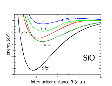
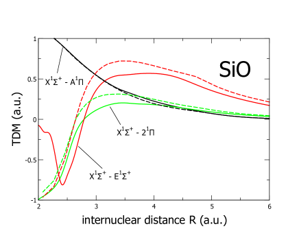
Figure 1: (Colour online) SiO, a comparison of the potentials energy curves (PEC’s) and transition dipole moments (TDM’s), as a function of internuclear distance $R$ (a.u.), from paper I (Forrey et al., 2016) (solid curves, MRCI + Q, AV6Z basis) with the recent molecular electronic structure calculations of Bauschlicher (2016) (dashed curves, IC-MRCI, AV5Z basis). See text for further details.

2 Theory

We describe two methods for calculating the rate constant. Both methods utilize a Sturmian representation to form a complete basis set for both the dynamics and kinetics (Forrey, 2013, 2015). Following paper I, the RA cross section is defined by

$$\sigma_{\Lambda\rightarrow\Lambda^{\prime}}(E)=\frac{\pi^{2}\hbar^{3}}{\mu E}P_{\Lambda}\sum_{b,u}(2j_{u}+1)(1+\delta_{u})\,\Gamma_{u\rightarrow b}^{rad}\,\delta(E-E_{u}),$$ (4)

where $\Lambda$ and $\Lambda^{\prime}$ are initial and final projections of the electronic orbital angular momentum of the molecule on the internuclear axis, $\mu$ is the reduced mass of the Si+O system, and $E$ is the translational energy. Here $b\equiv(v_{b},j_{b})$ and $u\equiv(v_{u},j_{u})$ designate vibrational and rotational quantum numbers for bound and unbound states, respectively. $\Gamma_{u\rightarrow b}^{rad}$ is the probability for a radiative transition between the unit-normalized states, and $\delta_{u}$ is a dimensionless parameter which may be computed within a given kinetic model to obtain the density of unbound states. The statistical factor

$$P_{\Lambda}=\frac{(2S_{mol}+1)(2-\delta_{0,\Lambda})}{(2L_{Si}+1)(2S_{Si}+1)(2L_{O}+1)(2S_{O}+1)}\$$ (5)

is determined by $L_{Si}$, $S_{Si}$, $L_{O}$, and $S_{O}$, the electronic orbital and spin angular momenta of the silicon and oxygen atoms, and $S_{mol}$ the total spin of the molecular electronic state.

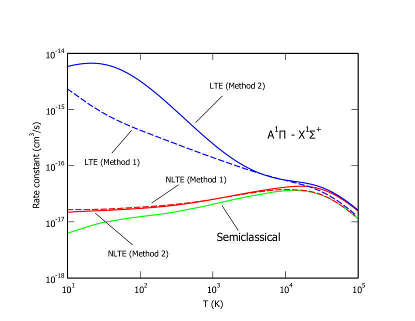
Figure 2: (Colour online) Radiative association rate constants (cm³/s) as a function of temperature $T$ (K) for the $A^{1}\Pi\rightarrow X^{1}\Sigma^{+}$ transition in SiO. Method 1 refers to the analytical evaluation of the thermal average in equation (6) which yields equation (8). Method 2 refers to numerical integration of the thermal average in equation (6). Both methods used a Sturmian basis set of 500 functions. Full convergence was obtained for Method 1. The convergence rate for Method 2 is much slower, particularly for the LTE curve which oscillates above the converged value. It is seen that both methods converge to the semiclassical result at higher temperatures, where resonance effects are no longer important.

The thermally averaged rate constant is defined by

$$k_{\Lambda\rightarrow\Lambda^{\prime}}=\frac{1}{2\pi Q_{T}}\int_{0}^{\infty}E\;\sigma_{\Lambda\rightarrow\Lambda^{\prime}}(E)\;e^{-E/k_{B}T}dE\ ,$$ (6)

where

$$Q_{T}=\mbox{$\left(\frac{2\pi\hbar^{2}}{\mu k_{B}T}\right)$}^{-3/2}$$ (7)

is the translational partition function for temperature $T$ and $k_{B}$ is Boltzmann’s constant. Method 1 performs the thermal average analytically by substituting (4) into (6) to obtain the rate constant

$$k_{\Lambda\rightarrow\Lambda^{\prime}}=\sum_{b,u}\,K_{u}^{eq}\,(1+\delta_{u})\,\Gamma_{u\rightarrow b}^{rad}$$ (8)

in terms of the equilibrium constant

$$K_{u}^{eq}=\frac{(2j_{u}+1)P_{\Lambda}\exp(-E_{u}/k_{B}T)}{Q_{T}}\ .$$ (9)

This method does not require computation of the cross section. Method 2 performs the thermal average numerically using $\delta(E-E_{u})=\delta_{E,E_{u}}/w_{E}$ to calculate the cross section. Here $w_{E}$ is the equivalent quadrature weight which transforms the unit-normalized state to energy-normalization. The weights depend on $j_{u}$ and may be obtained from the energy spectrum of the free Hamiltonian using the Heller derivative method (Heller, 1973). The Kronecker delta function reduces equation (4) to a single sum over bound states for an energy grid comprised of unbound eigenstates of the interacting Hamiltonian. These unbound eigenstates include quasi-bound states and discretized continuum states, so the direct process (2) and the indirect process (3) are both fully accounted for in the Sturmian formulation. Rate constants are computed by interpolating the cross section (4) over the energy grid and numerically integrating equation (6).

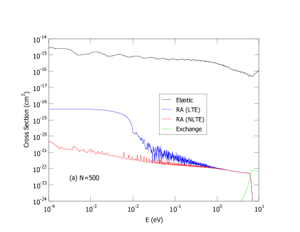
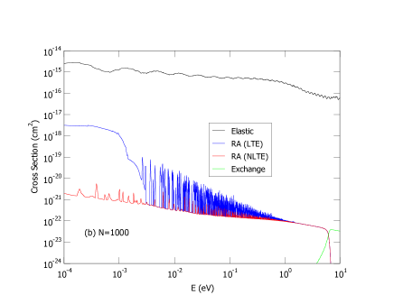
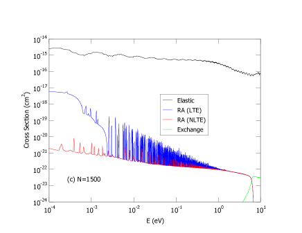
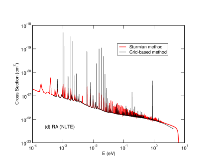
Figure 3: (Colour online) Cross sections for elastic scattering, RA, and radiative exchange for approach on the $A^{1}\Pi$ potential. The calculations used Sturmian ${\cal L}^{2}$ basis sets with (a) 500, (b) 1000, and (c) 1500 functions. The resonances become better resolved and more densely populated as the size of the basis set is increased. The RA (NLTE) cross section in (c) is compared against a numerical grid-based method in (d). The peaks of the resonances are modulated by the kinetic parameters for the Sturmian ${\cal L}^{2}$ method but not for the quantum grid-based method.

The radiative width generally includes spontaneous and stimulated emission and may be written

$$\Gamma_{u\rightarrow b}^{rad}=\frac{A_{u\rightarrow b}}{1-e^{-(E_{u}-E_{b})/k_{B}T_{R}}}$$ (10)

for a pure blackbody radiation field with temperature $T_{R}$. The kinetic parameter $\delta_{u}$ is determined by the conditions of the gas. For a gas in LTE, the full parameter set is defined by $\delta_{u_{i}}=0$. For a NLTE-ZDL gas ($T_{R}=0$), the parameter set is determined by the formula (Forrey, 2015)

$$1+\delta_{u_{i}}=\frac{1}{1+\tau_{u_{i}}\left(\sum_{j<i}A_{u_{i}\rightarrow u_{j}}+\sum_{j}A_{u_{i}\rightarrow b_{j}}\right)}$$ (11)

where

$$\tau_{u_{i}}^{-1}=2\pi|\langle u_{i}|V|f\rangle|^{2}$$ (12)

is the tunneling width, and $f$ is an energy-normalized free eigenstate with the same energy as the interacting unbound state. The Einstein A-coefficients are given by

$$A_{u_{i}\rightarrow b_{j}}=\frac{4}{3c^{3}}(E_{u_{i}}-E_{b_{j}})^{3}S_{j_{u_{i}}j_{b_{j}}}|\langle u_{i}|M|b_{j}\rangle|^{2}$$ (13)

and similarly for $A_{u_{i}\rightarrow u_{j}}$, where $S_{j,j^{\prime}}$ are the appropriate line strengths (Cowan, 1981; Curtis, 2003) or Hönl-London factors (Watson, 2008), and $c$ is the speed of light. The electronic dipole moment is defined by

$$M=\left\{\begin{array}[]{cc}\langle\psi_{e}|p_{z}|\psi_{e}^{\prime}\rangle&\ \ \Lambda=\Lambda^{\prime}\\ \frac{1}{\sqrt{2}}\langle\psi_{e}|p_{x}+ip_{y}|\psi_{e}^{\prime}\rangle&\ \ \Lambda\neq\Lambda^{\prime}\end{array}\right.$$ (16)

where $(p_{x},p_{y},p_{z})$ are the components of the dipole operator and $\psi_{e}$ is the electronic wave function. We note that the $\frac{1}{\sqrt{2}}$ normalization in (16) was double-counted in paper I for the $A^{1}\Pi$ to $X^{1}\Sigma^{+}$ transition. The radiative and tunneling widths have been calculated for all of the initial SiO electronic states considered in the present work.

3 Results

The molecular electronic structure calculations used in the present work were reported on in paper I. In that work a multi-reference configuration-interaction approximation was used with the Davidson correction (MRCI +Q) and an aug-cc-pV6Z basis. The molecular orbitals were determined using the state-averaged-complete-active-space-self-consistent field (SA-CASSCF) approximation. Where necessary we have included updated details of those molecular electronic structure calculations in the present work. Recently, Bauschlicher (2016) reported similar calculations using the internally-contracted multi-reference configuration-interaction (IC-MRCI) approximation with an aug-cc-pV5Z basis set with the molecular orbitals (MO’s) obtained from dynamically-weighted (DW) CASSCF calculations.

In both paper I and Bauschlicher (2016) the molpro quantum chemistry suite of molecular structure codes (Werner et al., 2015) were used. The molecular constants for several low-lying states in SiO are compared with those obtained from the work of Bauschlicher (2016) and previous theoretical and experimental work in Table 1. Good agreement is found in all cases. The largest discrepancy occurs for the bond distances for the $A^{1}\Pi$ and $E^{1}\Sigma^{+}$, being $\sim$0.01 and 0.02 Å larger than experiment, respectively.

A comparison of the PEC’s and TDM’s for the two sets of calculations is illustrated in Figure 1. The solid curves correspond to the data from paper I and the dashed curves to the data from Bauschlicher (2016). The PEC’s are in excellent agreement for the $X^{1}\Sigma^{+}$ and $A^{1}\Pi$ states, and the agreement is also very good for the $E^{1}\Sigma^{+}$ and $2^{1}\Pi$ electronic states. However, we note there is a small disagreement in the region around 4 – 5 a.u. Both calculations show a small potential barrier for the $2^{1}\Pi$ state. Bauschlicher (2016) reported no barrier for this state, however, the data provided to us by the author contains a small barrier of about 0.3 eV, compared to a barrier height of 0.4 eV found in this work. The TDM’s show good quantitative agreement for the $X^{1}\Sigma^{+}$ to $A^{1}\Pi$ transition, and qualitative agreement for the $X^{1}\Sigma^{+}$ to $E^{1}\Sigma^{+}$ and $X^{1}\Sigma^{+}$ to $2^{1}\Pi$ transitions.

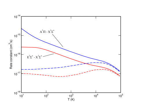
Figure 4: (Colour online) Radiative association rate constants for the $E^{1}\Sigma^{+}\rightarrow X^{1}\Sigma^{+}$, and $A^{1}\Pi\rightarrow X^{1}\Sigma^{+}$ transitions in SiO. Solid curves correspond to LTE and dashed curves to NLTE.

Radiative lifetimes for the $A^{1}\Pi$, $E^{1}\Sigma^{+}$, and $2^{1}\Pi$ states are presented in Table 2. These lifetimes were computed by summing equation (13) over all bound levels. Excellent agreement with previous calculations (Chattopadhyaya et al., 2003; Bauschlicher, 2016) is found for the $A^{1}\Pi$ state, however, the agreement is poor for the other states. This may be due in small part to the differences in the potential curves noted above. The larger contribution to the discrepancy is attributable to the differences in the TDM’s. The comparison given in Figure 1 for the $E^{1}\Sigma\rightarrow X^{1}\Sigma^{+}$ and $2^{1}\Pi\rightarrow X^{1}\Sigma^{+}$ transitions shows that the TDM’s from paper I have magnitudes that are smaller than those of Bauschlicher (2016) by amounts which are consistent with the discrepancies in Table 2.

Table 1: Equilibrium bond distance $R_{e}$ (Å) and dissociation energies $D_{e}$ (eV) for the $X^{1}\Sigma^{+}$, $D^{1}\Delta$, $A^{1}\Pi$, $E^{1}\Sigma^{+}$, and $2^{1}\Pi$ states of SiO for the present MRCI+Q calculations compared to other theoretical and experimental results. (The data are given in units conventional to quantum chemistry with 1 Å=$10^{-10}$ m and $0.529177$ Å $\approx a_{0}$. The conversion factor $1.239842\times 10^{-4}$ eV = 1 $\mathrm{cm}^{-1}$ is also used.)

State	Method	$R_{e}/$Å	$D_{e}/\mathrm{eV}$
$X^{1}\Sigma^{+}$
	MRCI+Qa	1.5153	8.2748
	IC-MRCIb	1.5170	8.3277
	MRCI+Qc	1.5100	8.3776
	MRDCId	1.5210	–
	Experimente	1.5097	8.3368
	Experimentf	–	8.26 $\pm$ 0.13
	Experimentg	–	8.33 $\pm$ 0.09
	Experimenth	1.5100	8.18 $\pm$ 0.03
$D^{1}\Delta$
	MRCI+Qa	1.7399	3.4866
	IC-MRCIb	1.7395	3.5359
	MRDCId	1.7440	–
	Experimente	1.7290	–
	Experimentj	1.7270	–
$A^{1}\Pi$
	MRCI+Qa	1.6315	2.9693
	IC-MRCIb	1.6339	2.9629
	MRCI+Qc	1.6229	3.0510
	MRDCId	1.6500	–
	Experimente	1.6206	3.0259
	Experimentg	1.6200	2.87 $\pm$ 0.03
	Experimenti	1.6199	–
	Experimentj	1.6207	–
$E^{1}\Sigma^{+}$
	MRCI+Qa	1.7625	1.8177
	IC-MRCIb	1.7415	1.7823
	MRDCId	1.7550	–
	Experimente	1.7398	–
	Experimenti	1.7399	–
$2^{1}\Pi$
	MRCI+Qa	1.7650	0.5808
	IC-MRCIb	1.7281	0.6018
	MRDCId	1.7050	–
	Experimentj	–	–

^aMulti-reference configuration interaction (MRCI) and Davidson correction (+Q), aug-cc-pV6Z basis, present work

^bInternally contracted multi-reference configuration interaction (IC-MRCI), aug-cc-pV5Z basis (Bauschlicher, 2016)

^cMulti-reference configuration interaction (MRCI) and Davidson correction (+Q), aug-cc-pV6Z (Shi et al., 2012)

^dMRDCI, basis, Si (7s6p5d2f/7s6p4d1f), O(4s4p1d) (Chattopadhyaya et al., 2003)

^eExperiment (Huber & Herzberg, 1979)

^fExperiment (Hildenbrand, 1972)

^gExperiment (Brewer & Rosenblatt, 1969)

^hExperiment (Gaydon, 1968)

ⁱExperiment (Lagerqvist et al., 1973)

^jExperiment (Field et al., 1976)

We interpolated the ab initio calculated PEC’s and TDM’s using cubic splines. For $R<$ 1.5 $\mathrm{a}_{0}$, the ab initio data was joined smoothly to the analytic form $a\exp(bR)$, where $a$ and $b$ for each state were determined by fitting. For $R>$ 20 $\mathrm{a}_{0}$, the appropriate long-range forms were used for the separating atoms. In particular, for Si(${}^{3}P$) + O(${}^{3}P$), this corresponds to having dispersion coefficients for the $C_{5}/R^{5}$ and $C_{6}/R^{6}$ terms. The $C_{6}$ dispersion coefficients were determined using the Slater & Kirkwood (1931) formula,

$$C_{6}=\frac{3}{2}\frac{\alpha_{A}\alpha_{B}}{\sqrt{\alpha_{A}/N_{A}}+\sqrt{\alpha_{B}/N_{B}}}$$ (17)

where $\alpha_{A}$ and $\alpha_{B}$ are the dipole polarisability with $N_{A}$ and $N_{B}$ the number of equivalent electrons of the Si and O atoms, respectively. This yielded a value for $C_{6}$ of 53.67 a.u for the states separating to Si(${}^{3}P$) + O(${}^{3}P$), which is in suitable agreement with the value of 63.3 a.u. determined from the London formula, where $C_{6}$ is determined via

$$C_{6}=\frac{3}{2}\frac{{\cal I}_{A}{\cal I}_{B}}{[{\cal I}_{A}+{\cal I}_{B}]}{\alpha_{A}\alpha_{B}}$$ (18)

with ${\cal I}_{A}$ and ${\cal I}_{B}$ being the first ionization energies of the separated atoms A and B. The $C_{5}$ dispersion coefficients were estimated using the approach outlined in Chang (1967), which respectively gave values for the $X^{1}\Sigma^{+}$ state of 25.5 a.u, the $A^{1}\Pi$ and $E^{1}\Sigma^{+}$ states are 0.0, the $D^{1}\Delta$ state is 4.25 a.u and the $2^{1}\Pi$ state is $-17.0$ a.u.

Table 2: SiO, radiative lifetimes $\tau$ (ns) for the $v=0,j=0$ level of the upper electronic state.

SiO ro-vibrational transition	$\tau$ (ns)	$\tau$ (ns)	$\tau$ (ns)
($v=0,j=0\rightarrow v^{\prime},j^{\prime}$)	CWBa	CCDb	Present workc
$A^{1}\Pi\rightarrow X^{1}\Sigma^{+}$	28.9	29.3	29.5
$E^{1}\Sigma\rightarrow X^{1}\Sigma^{+}$	7.1	11.0	21.7
$2^{1}\Pi\rightarrow X^{1}\Sigma^{+}$	14.9	29.7	90.4

^aIC-MRCI, AV5Z basis (Bauschlicher, 2016)

^bMRDCI, (4s,4p,1d) basis (Chattopadhyaya et al., 2003)

^cMRCI + Q, AV6Z basis, present work

In paper I, the LTE rate constants included stimulated emission for an ideal blackbody radiation field with $T_{R}=T$. In the present work, we neglect stimulated emission and assume that thermalization is entirely due to collisions. This yields no difference between the two LTE definitions when $T<10^{4}$ K since the denominator of equation (10) is very close to unity for these temperatures. The rate constants defined here, however, are smaller than those in paper I for $T>10^{4}$ K. The results presented here also correct the double-counting error in equation (16) made in paper I for the $A^{1}\Pi\rightarrow X^{1}\Sigma^{+}$ transition.

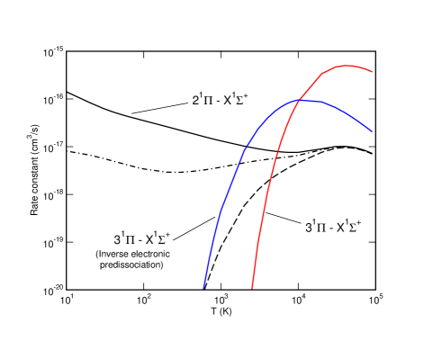
Figure 5: (Colour online) Radiative association rate constants for $2^{1}\Pi\rightarrow X^{1}\Sigma^{+}$ and $3^{1}\Pi\rightarrow X^{1}\Sigma^{+}$ transitions in SiO. Solid curves correspond to LTE and broken curves to NLTE-ZDL. The dashed broken curve, which uses only the tunneling widths for the $2^{1}\Pi$ potential, shows a threshold due to a barrier in the potential. The dot-dashed curve includes tunneling widths from the $A^{1}\Pi$ potential, which removes the threshold for the $2^{1}\Pi$ rate constant. The rate constants for the $3^{1}\Pi$ state have thresholds that are due to the asymptotic shift in the potential. The red curve corresponds to approach on the $3^{1}\Pi$ state. The blue curve corresponds to a radiation-less transition from the $A^{1}\Pi$ state to an intermediate bound level of the $3^{1}\Pi$ state prior to radiative decay to the $X^{1}\Sigma^{+}$ state.

The RA rate constants for the $A^{1}\Pi\rightarrow X^{1}\Sigma^{+}$ contribution were computed using both Sturmian methods described above. Figure 2 shows that the NLTE-ZDL curves for the two methods are in reasonable agreement with each other and with the semiclassical calculation. Method 1 is in near perfect agreement with the semiclassical result at high temperatures. The LTE and NLTE curves for both methods merge together at high temperature due to the diminishing importance of the resonant contribution. Discrepancies between Method 1 and Method 2 are due to the different rates of convergence of the two methods. Both methods used 500 Sturmian basis functions to obtain the rate constants shown in Figure 2. Full convergence was achieved for Method 1. The convergence rate for Method 2, however, is much slower.

The LTE rate constant for Method 2 appears to oscillate above the converged value given by Method 1. This is due to interpolating the narrow high-$j_{u}$ resonances at low energies where the energy level spacing of the Sturmian eigenvalues is relatively large. As a result, an artificial step-like structure is obtained in the cross sections at low energies. This step goes away as the size of the basis set is increased. Figure 3 shows our results for basis sets consisting of 500, 1000, and 1500 functions. The largest calculation for Method 2, which is computationally inefficient, has still not reached the level of convergence obtained by Method 1 using far fewer basis functions.

The LTE curve converges more slowly than the NLTE curve for Method 2 due to the enhanced importance of the resonances. This is demonstrated in Figure 3 which shows cross sections for elastic scattering, RA, and radiative exchange (approach on the $A^{1}\Pi$ curve and exit on the $X^{1}\Sigma^{+}$ curve) which is negligible except at very high energies. The elastic cross section is computed using

$$\sigma_{el}(E)=\frac{\pi^{2}\hbar^{2}}{\mu E}P_{\Lambda}\sum_{u}(2j_{u}+1)(1+\delta_{u})\,\tau_{u}^{-1}\,\delta(E-E_{u}).$$ (19)

As expected, the elastic cross section is substantially larger than the RA cross section for all energies. Tunneling and radiative widths are computed using equations (12) and (13). These are used in equation (11) to obtain the set of kinetic parameters $\delta_{u_{i}}$ which are needed to describe the deviation from LTE. The kinetic parameter set is then substituted into equations (4) and (19) to obtain the NLTE-ZDL cross sections. Figure 3 shows that the kinetic parameters have a dramatic effect on the resonant contribution to the cross section. Whereas the non-resonant background contribution converges rapidly with basis set size, the resonant contribution becomes better resolved and more densely populated as the size is increased. This is particularly evident in the LTE curve which shows resonant enhancements that are typically 100 times larger than the NLTE-ZDL curve. As shown in Figure 2 when the cross sections are numerically integrated to obtain RA rate constants, the LTE and NLTE-ZDL curves differ by about a factor of 100 at low temperatures where the resonances are most important. The slow convergence of the LTE rate constant illustrates the difficulties associated with numerically resolving and integrating narrow resonances.

In the Sturmian theory (Forrey, 2013, 2015), the heights of the resonant peaks are determined by the kinetic parameters $\delta_{u}$. This is not the case for perturbation theory approaches which use a grid-based numerical method to solve the Schrödinger equation for the continuum wavefunction. Figure 3(d) compares the RA (NLTE-ZDL) cross section in (c) with the same cross section obtained by a grid-based perturbative method. Clearly, the agreement between the two methods is excellent for the broad resonances and non-resonant background. As expected, the grid-based method appears to miss some of the narrow resonances in the dense region around and above 0.1 eV, and the narrow resonant peaks show variable heights. Both of these issues are related to the relative spacing of the energy grid. A fine energy-spacing is needed to resolve the narrow resonances, however, this can yield unphysically high resonant peaks such as those seen in the figure. Many of these peaks are higher than the corresponding NLTE-ZDL peaks and are examples of the so-called breakdown of perturbation theory that occurs when the opacity violates unitarity (Antipov et al., 2013; Bennett et al., 2003). The set of kinetic parameters obtained from equation (11) ensures unitarity for a NLTE-ZDL gas and is equivalent to conventional methods which use radiative broadening to rescale the peaks of narrow resonances (Bain & Bardsley, 1972; Antipov et al., 2013; Bennett et al., 2003; Mrugala et al., 2003).

Due to the faster convergence rate and convenience of bypassing the computation of the cross section, we used Method 1 for the remaining calculations. The basis sets used 500 Sturmian functions with a scale factor of 75 a.u. All of the tunneling and radiative widths needed to evaluate equation (11) were computed and used in equation (8) to obtain the RA rate constants. Figure 4 shows the rate constants for $E^{1}\Sigma^{+}\rightarrow X^{1}\Sigma^{+}$, and $A^{1}\Pi\rightarrow X^{1}\Sigma^{+}$ transitions. The solid curves correspond to LTE and the dashed curves to NLTE-ZDL. The $E^{1}\Sigma^{+}\rightarrow X^{1}\Sigma^{+}$ contribution is seen to be comparable to the $A^{1}\Pi\rightarrow X^{1}\Sigma^{+}$ contribution. In both cases, the LTE and NLTE-ZDL curves are well-separated at low temperature and gradually approach each other as the temperature is increased due to the diminishing importance of the resonances.

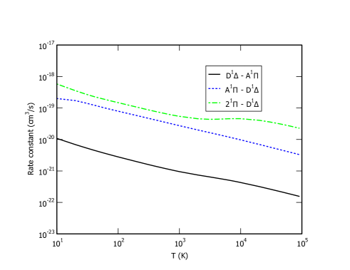
Figure 6: (Colour online) Radiative association rate constants for transitions in SiO. The dashed line (blue) is $A^{1}\Pi\rightarrow D^{1}\Delta$, dot dashed line (green) $2^{1}\Pi\rightarrow D^{1}\Delta$, and the solid line (black) is $D^{1}\Delta\rightarrow A^{1}\Pi$

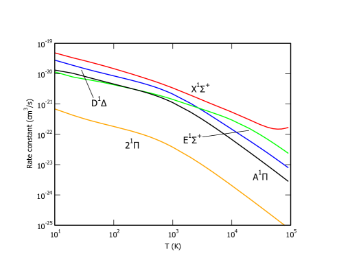
Figure 7: (Colour online) Radiative association rate constants due to permanent dipoles for $X^{1}\Sigma^{+}$, $D^{1}\Delta$, $E^{1}\Sigma^{+}$, $A^{1}\Pi$, and $2^{1}\Pi$ in SiO.

Figure 5 shows RA rate constants for the $2^{1}\Pi\rightarrow X^{1}\Sigma^{+}$ and the $3^{1}\Pi\rightarrow X^{1}\Sigma^{+}$ transitions. Qualitatively similar behaviour is observed for the $2^{1}\Pi$ and $A^{1}\Pi$ LTE curves. Two NLTE-ZDL curves are shown for the $2^{1}\Pi$ state. The dashed curve corresponds to calculations which include tunneling widths (12) for the $2^{1}\Pi$ potential. This curve shows a strong threshold effect due to a barrier in the potential curve (Chattopadhyaya et al., 2003; Forrey et al., 2016), which prevents low energy collisions from approaching close separations where the TDM is largest. The $2^{1}\Pi$ potential of Bauschlicher (2016) has a somewhat smaller barrier suggesting some uncertainty in the rate constant given by the dashed curve. The dot-dashed curve corresponds to calculations which include tunneling widths (12) for both the $2^{1}\Pi$ and the $A^{1}\Pi$ potentials. Since the $A^{1}\Pi$ potential has no barrier, the threshold is removed and the NLTE-ZDL rate constant appears more in-line with those presented in Figure 4.

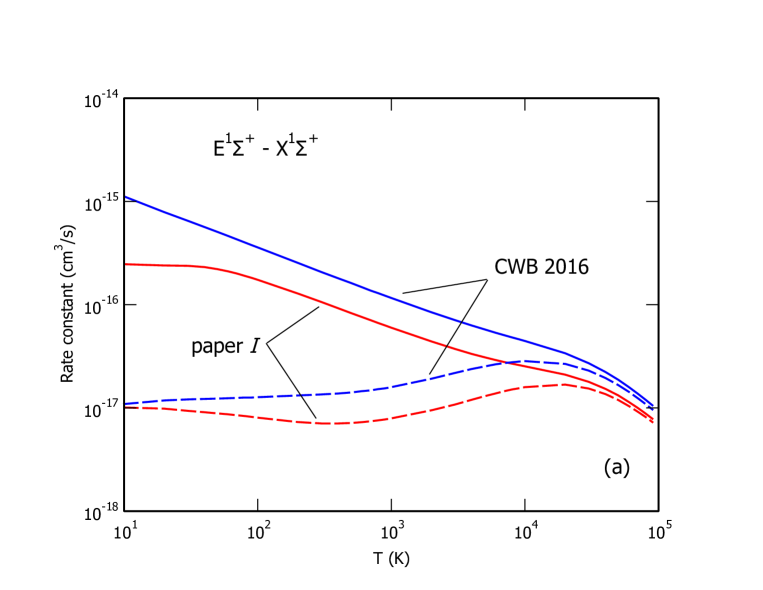
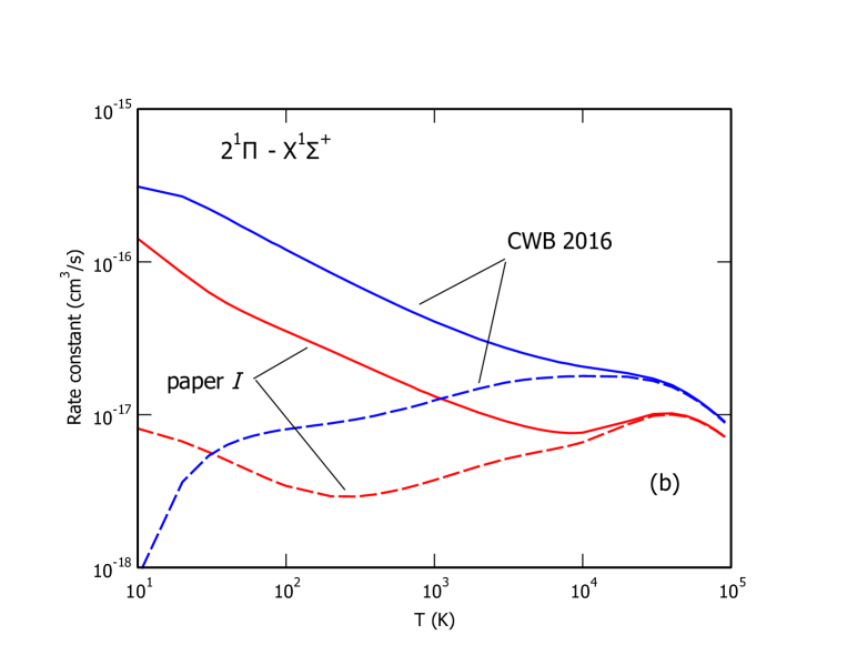
Figure 8: (Colour online)A comparison of the rate constants using the molecular data for PEC’s and TDM’s from paper I (Forrey et al., 2016), (red curves) and that from Bauschlicher (2016), (blue curves). (a) $E^{1}\Sigma^{+}\rightarrow X^{1}\Sigma^{+}$ and (b) $2^{1}\Pi^{+}\rightarrow X^{1}\Sigma^{+}$ transitions in SiO. Solid lines in both cases correspond to LTE and dashed lines to NLTE-ZDL.

Figure 5 also shows two RA contributions from the $3^{1}\Pi$ state. The $3^{1}\Pi$ state separates at long internuclear distance to Si(${}^{1}D$)+O(${}^{1}D$), which is shifted from the Si(${}^{3}P$)+O(${}^{3}P$) asymptote by 2.7 eV. This produces a threshold for RA via the $3^{1}\Pi$ state (red curve) which is at a sufficiently high energy such that resonances do not make a substantial contribution, and that the LTE and NLTE-ZDL rate constants are virtually identical. It should be noted that the $3^{1}\Pi$ state also allows RA to take place through inverse electronic predissociation. In this process, bound ro-vibrational levels of the $3^{1}\Pi$ state are populated by approach on the $A^{1}\Pi$ state, characterized by the tunneling widths (12). Subsequently, the bound levels of the $3^{1}\Pi$ state can decay to the $X^{1}\Sigma^{+}$ in a similar manner to the quasi-bound rotational states which contribute to RA through inverse rotational predissociation. When the translational energy of the approaching atoms is large enough to match the energy of the bound levels of the $3^{1}\Pi$ state, the rate constant is non-zero and rises rapidly (blue curve). It is noteworthy that the bottom of the potential well for the $3^{1}\Pi$ state has an energy which is approximately the same as the energy of the potential barrier for the $2^{1}\Pi$ state. This causes the threshold for the $3^{1}\Pi$ inverse electronic predissociation curve to be at about the same temperature as the threshold for the $2^{1}\Pi$ NLTE-ZDL curve. The relatively large maximum for the red $3^{1}\Pi$ curve is due to large energy differences involved in the radiative transitions, and the replacement of $P_{\Pi}=2/81$ with $P_{\Pi}=2/25$ due to the different atomic asymptotes. The blue $3^{1}\Pi$ curve does not undergo this statistical replacement since the atoms approach each other on the $A^{1}\Pi$ state.

Table 3: Parameters for the analytic formula (21) used to fit the SiO rate coefficients as a function of temperature $T$ (K) over the range 10 – 10,000 K.

Fitting		$A^{1}\Pi\rightarrow X^{1}\Sigma^{+}$		$E^{1}\Sigma\rightarrow X^{1}\Sigma^{+}$		$2^{1}\Pi\rightarrow X^{1}\Sigma^{+}$
parameter	LTE	NLTE-ZDL	LTE	NLTE-ZDL	LTE	NLTE-ZDL
$a$	2.08233	0.222128	0.816526	0.0846568	0.244134	0.0360735
$b$	0.420491	$-$0.161335	0.373286	$-$0.0982334	0.488114	$-$0.168372
$c_{1}$	481.186	5.71969	879.858	7.91451	$-$174.301	9.10961
$c_{2}$	0	0	$-$8.44818	$-$1191.94	$-$695.992	$-$237.498
$c_{3}$	0	0	$-$21.8148	273212	150707	11728.5
$d_{1}$	1.37764	14.09	78.2256	18.4612	45.4479	15.4816
$d_{2}$	0	0	0.3277	830.387	388.013	536.223
$d_{3}$	0	0	3.05515	19999.8	18243.8	12844.6

Figure 6 shows RA rate constants for $A^{1}\Pi\rightarrow D^{1}\Delta$, $2^{1}\Pi\rightarrow D^{1}\Delta$, and $D^{1}\Delta\rightarrow A^{1}\Pi$ transitions. These rate constants are smaller than those which lead to the formation of bound states for the $X^{1}\Sigma^{+}$ potential. The $A^{1}\Pi$, $D^{1}\Delta$, and $E^{1}\Sigma^{+}$ potentials also support bound states, however, the dissociation energies of these electronic states are less than that of the $X^{1}\Sigma^{+}$. Consequently, the $(\Delta E)^{3}$ factor in equation (13) is not as large and the RA rate constants are smaller. The three curves shown in Figure 6 are the largest among all transitions which do not include $X^{1}\Sigma^{+}$ bound states. These curves represent the LTE rate constants; the NLTE-ZDL rate constants have the usual fall-off behaviour with decreasing temperature and are not shown. RA rate constants for $D^{1}\Delta$ to $E^{1}\Sigma^{+}$ and $X^{1}\Sigma^{+}$ to $A^{1}\Pi$, $D^{1}\Delta$, and $E^{1}\Sigma^{+}$ were computed and found to be smaller than $10^{-25}$ cm³/s.

Figure 7 shows permanent dipole contributions for the $X^{1}\Sigma^{+}$, $E^{1}\Sigma^{+}$, $A^{1}\Pi$, $2^{1}\Pi$, and $D^{1}\Delta$ states. Again, only the LTE rate constants are shown due to the relatively small values of the NLTE-ZDL rate constants at low temperatures. The LTE rate constants are comparable in magnitude to the transition dipole contributions shown in Figure 6.

Having considered all possible RA contributions, it is clear that formation of SiO is dominated by the $A^{1}\Pi$, $E^{1}\Sigma^{+}$, and $2^{1}\Pi$ states at low temperatures, and by the $3^{1}\Pi$ state at high temperatures. In order to estimate the uncertainty in the RA rate constants for these states, we compare results using the molecular data of Bauschlicher (2016) with those obtained using data from paper I. As expected from the comparisons shown in Figure 1, the rate constants for the $A^{1}\Pi$ to $X^{1}\Sigma^{+}$ transition were virtually identical, so the comparison is not shown. The $E^{1}\Sigma^{+}$ to $X^{1}\Sigma^{+}$ and $2^{1}\Pi$ to $X^{1}\Sigma^{+}$ comparisons are shown in Figure 8. Consistent with the lifetimes presented in Table 2, the RA rate constants calculated with the molecular data of Bauschlicher (2016) tend to be about 2-3 times larger than those obtained using the molecular data from paper I. It should be noted that the appropriate long-range forms for each state were included for the molecular curves from paper I but not for the CWB potentials. The rate constants are found to be sensitive to the long-range for $T<100$ K (see supplementary material). The enhanced sensitivity of the NLTE-ZDL rate constant in Figure 8(b) is due to the barrier in the 2${}^{1}\Pi$ potential and the coupling to the A${}^{1}\Pi$ state.

4 Summary and Conclusions

Two methods were used to compute RA rate constants for $A^{1}\Pi$ to $X^{1}\Sigma^{+}$ transitions. Both methods employed Sturmian basis sets to represent the bound and unbound ro-vibrational states. Results for the two methods are found to be in good agreement, however, Method 1 converges more rapidly and does not require calculation of the cross section. This method was subsequently used to calculate LTE and NLTE-ZDL rate constants for the low-lying electronic states of SiO. The LTE rate constants assume that all unbound states, including long-lived quasi-bound states, are populated by a Boltzmann equilibrium distribution. The NLTE-ZDL rate constants refer to a dilute gas at $T_{R}=0$ which have no excitation mechanisms. More general NLTE environments which have some collisional and/or radiative excitation capability would presumably have rate coefficients which lie somewhere in-between the NLTE-ZDL and LTE curves.

In light of the expectation that the true formation rate constant lies in-between the LTE and NLTE-ZDL values, it is tempting to provide a formula which interpolates between the two limits. This approach has been adopted previously (Lepp & Shull, 1983; Martin et al., 1996; Glover & Abel, 2008) for interpolating collision-induced dissociation rates between low and high density.

However, it should be noted, that there are two distinct ways to achieve the LTE results given here. The first assumes that the density is large enough that the quasi-bound states may be populated by three-body collisions. In this case, the total recombination rate constant

$$k_{r}=k_{r}^{(2)}+k_{r}^{(3)}n$$ (20)

would likely be dominated by the TBR contribution $k_{r}^{(3)}$. Therefore, the LTE RA rate constant $k_{r}^{(2)}$ may be used to estimate the TBR rate at the critical density $n_{cr}$, and it is possible that an interpolating scheme between low and high densities would be useful. The second way to achieve the LTE RA rate constant is to assume a pure blackbody radiation field with $T_{R}=T$ (Forrey, 2015). Realistic radiation fields are generally less intense than a pure blackbody field, so a formula for interpolating between $T_{R}=0$ and $T_{R}=T$ would need to account for the dilution. See Ramaker & Peek (1979) for an example where such an approach would be useful.

A simpler approach would be to use both the LTE and NLTE-ZDL rate constants in separate calculations to provide theoretical error bars in any model which depends on the SiO formation rate. To facilitate this approach, we provide analytic fitting functions (Novotný et al., 2013; Vissapragada et al., 2016) for both LTE and NLTE-ZDL rate constants using the form

$$k_{r}=\left[a(400/T)^{b}+T^{-3/2}\sum_{i=1}^{3}c_{i}\exp(-d_{i}/T)\right]\times 10^{-16}\ \mbox{cm}^{3}/\mbox{s}$$ (21)

where the parameters are given in Table 3. This formula provides a fit to the rates to better than 10 percent over the temperature range 10 – 10,000 K. A plot which compares the fitted rates with the calculated rates is included in the supplemental material. Also included in the supplementary data are the molecular data used to compute the rates. The primary source of error in the calculations is due to the TDM uncertainties (see Fig. 1b) which yield rate constants that differ by 2-3 times over the temperature range considered.

References

- Andreazza et al. (1995) Andreazza C. M., Singh P. D., Sanzovo G. C., 1995, ApJ, 451, 889
- Antipov et al. (2013) Antipov S. V., Gustafsson M., Nyman G., 2013, MNRAS, 430, 946
- Bain & Bardsley (1972) Bain R. A., Bardsley J. N., 1972, J. Phys. B: At. Mol. Phys., 5, 277
- Bates (1951) Bates D. R., 1951, MNRAS, 111, 303
- Bauschlicher (2016) Bauschlicher Jr. C. W., 2016, Chem. Phys. Lett., 658, 76
- Bennett et al. (2003) Bennett O. J., Dickinson A. S., Leininger T., Gadéa X., 2003, MNRAS, 341, 361
- Brewer & Rosenblatt (1969) Brewer K., Rosenblatt G. M., 1969, in Eyring L., ed., , Vol. 2, Advances in High-Temperature Chemistry. Academic, New York, USA, pp 1–81
- Chang (1967) Chang T. Y., 1967, Rev. Mod. Phys., 39, 911
- Chattopadhyaya et al. (2003) Chattopadhyaya S., Chattopadhyay A., Das K. K., 2003, J. Phys. Chem. A, 107, 148
- Cherchneff (2006) Cherchneff I., 2006, A&A, 456, 1001
- Cherchneff (2012) Cherchneff I., 2012, A&A, 545, A12
- Cooley (1961) Cooley J. W., 1961, Math. Comput., 15, 363
- Cowan (1981) Cowan R. D., 1981, The Theory of Atomic Structure and Spectra. University of California Press, Berkeley, California, USA
- Curtis (2003) Curtis L. J., 2003, Atomic Structure and Lifetimes: A conceptual Approach. Cambridge University Press, Cambridge, UK
- Dalgarno et al. (1990) Dalgarno A., Du M. L., You J. H., 1990, ApJ, 349, 675
- Field et al. (1976) Field R. W., Lagerqvist A., Renhron I., 1976, Phys. Scripta, 14, 298
- Forrey (2013) Forrey R. C., 2013, Phys. Rev. A, 88, 052709
- Forrey (2015) Forrey R. C., 2015, J. Chem. Phys., 143, 024101
- Forrey et al. (2016) Forrey R. C., Babb J. F., Stancil P. C., McLaughlin B. M., 2016, J. Phys. B: At. Mol. Opt. Phys., 48
- Franz et al. (2011) Franz J., Gustafsson M., Nyman G., 2011, MNRAS, 414, 3547
- Gaydon (1968) Gaydon A. G., 1968, Dissociation energies and Spectra of Diatomic Molecules. Chamman and Hall, London, UK
- Gearhart et al. (1999) Gearhart R., Wheeler J., Swartz D., 1999, ApJ, 510, 944
- Glover & Abel (2008) Glover S. C. O., Abel T., 2008, MNRAS, 388, 1627
- Heller (1973) Heller E. J., 1973, PhD thesis, Harvard University
- Hildenbrand (1972) Hildenbrand D. L., 1972, H. Temp. Sci., 4, 244
- Huber & Herzberg (1979) Huber K. P., Herzberg G., 1979, Molecular Spectra and Molecular Structure IV: Constants of Diatomic Molecules. Van Nostrand-Reinhold, Princeton, New Jersey, USA
- Johnson (1977) Johnson B. R., 1977, J. Chem. Phys., 67, 4086
- Lagerqvist et al. (1973) Lagerqvist A., Renhron I., Elander N., 1973, J. Molec. Spectrosc., 46, 285
- Lepp & Shull (1983) Lepp S., Shull J. M., 1983, ApJ, 270, 578
- Lepp et al. (1990) Lepp S., Dalgarno A., McCray R., 1990, ApJ, 358, 262
- Li et al. (2014) Li X., Millar T. J., C. W., Heays A. N., van Dishoeck E. F., 2014, A&A, 568, A111
- Li et al. (2016) Li X., Millar T. J., Heays A. N., C. W., van Dishoeck E. F., Cherchneff I., 2016, A&A, 588, A4
- Liu & Dalgarno (1996) Liu W., Dalgarno A., 1996, ApJ, 471, 480
- Marassi et al. (2015) Marassi S., Schneider R., Limongi M., Chieffi A., Bocchio M., Bianchi S., 2015, MNRAS, 454, 4250
- Martin et al. (1996) Martin P. G., Schwarz D. H., Mandy M. E., 1996, ApJ, 461, 265
- Mrugala et al. (2003) Mrugala F., Spirko V., Kraemer W. P., 2003, J. Chem. Phys., 118, 10547
- Novotný et al. (2013) Novotný O., et al., 2013, ApJ, 777, 54
- Nyman et al. (2015) Nyman G., Gustafsson M., Antipov S. V., 2015, Int. Rev. Phys. Chem., 34, 385
- Öström et al. (2016) Öström J., Bezrukov D., Nyman G., Gustafsson M., 2016, J. Chem. Phys, 144, 044302
- Ramaker & Peek (1979) Ramaker D. E., Peek J. M., 1979, J. Chem. Phys., 71, 1844
- Rawlings & Williams (1989) Rawlings J. M. C., Williams D. A., 1989, MNRAS, 240, 729
- Shi et al. (2012) Shi D., Li W., Sun J., Zhu Z., 2012, Spectrochimica Acta Part A, 87, 96
- Slater & Kirkwood (1931) Slater J. C., Kirkwood J. G., 1931, Phys. Rev., 37, 682
- Stancil et al. (1993) Stancil P. C., Babb J. F., Dalgarno A., 1993, ApJ, 414, 672
- Vissapragada et al. (2016) Vissapragada S., Buzard C. F., Miller K. A., O’Connor A. P., de Ruette N., Urbain X., Savin D. W., 2016, ApJ, 832, 31
- Watson (2008) Watson J. K. G., 2008, J. Molec. Spectrosc., 253, 5
- Werner et al. (2015) Werner H. J., Knowles P. J., Manby F. R., Schütz M., Team 2015, molpro, http://www.molpro.net
- Willacy & Cherchneff (1998) Willacy K., Cherchneff I., 1998, A&A, 330, 676
- Zygelman & Dalgarno (1990) Zygelman B., Dalgarno A., 1990, ApJ, 365, 239