Simultaneous Monitoring of X-ray and Radio Variability in Sagittarius A*

Abstract

Monitoring of Sagittarius A* from X-ray to radio wavelengths has revealed structured variability — including X-ray flares — but it is challenging to establish correlations between them. Most studies have focused on variability in the X-ray and infrared, where variations are often simultaneous, and because long time series at sub-millimeter and radio wavelengths are limited. Previous work on sub-mm and radio variability hints at a lag between X-ray flares and their candidate sub-millimeter or radio counterparts, with the long wavelength data lagging the X-ray. However, there is only one published time lag between an X-ray flare and a possible radio counterpart. Here we report 9 contemporaneous X-ray and radio observations of Sgr A*. We detect significant radio variability peaking $\gtrsim$176 minutes after the brightest X-ray flare ever detected from Sgr A*. We also report other potentially associated X-ray and radio variability, with the radio peaks appearing $\lesssim$80 minutes after these weaker X-ray flares. Taken at face value, these results suggest that stronger X-ray flares lead to longer time lags in the radio. However, we also test the possibility that the variability at X-ray and radio wavelengths is not temporally correlated. We cross-correlate data from mismatched X-ray and radio epochs and obtain comparable correlations to the matched data. Hence, we find no overall statistical evidence that X-ray flares and radio variability are correlated, underscoring a need for more simultaneous, long duration X-ray–radio monitoring of Sgr A*.

=1

1 Introduction

Sagittarius A* (Sgr A*) is a presently dormant supermassive black hole at the dynamical center of our Galaxy, with a mass $M$ of $\sim 4\times 10^{6}$ $M_{\odot}$ (Schödel et al., 2002; Ghez et al., 2008; Gillessen et al., 2009). It has a very low accretion rate ($\lesssim$10^-7 $M_{\odot}\,{\rm yr}^{-1}$; Marrone et al. 2006; Shcherbakov et al. 2012; Yusef-Zadeh et al. 2015), and bolometric to Eddington luminosity ratio ($L/L_{Edd}$ $\sim$ 10^-9; Baganoff et al. 2003). This low $L/L_{Edd}$ can be understood in the context of a radiatively inefficient accretion flow (RIAF), such as an advection-dominated accretion flow (ADAF; Narayan et al., 1998; Yuan et al., 2003). At a distance of $\sim$8 kpc (Genzel et al., 2010; Boehle et al., 2016; Gillessen et al., 2017), Sgr A* is a prime target for studies of the physics and the environment of a low-accretion-rate SMBH (Falcke & Markoff, 2013).

For nearly two decades, beginning with the first detection of a flare in the X-ray (Baganoff et al., 2001), Sgr A* has been monitored for episodes of increased flux. Variability, which manifests as distinctive flares at high energies, has now been observed from X-ray to radio wavelengths. X-ray flaring detectable by Chandra occurs on average at a rate of 1.0$-$1.3 flares per day (Neilsen et al., 2013), although higher rates of X-ray flaring have been observed (Porquet et al., 2008; Neilsen et al., 2013; Ponti et al., 2015a; Mossoux & Grosso, 2017).

With variability occurring at all wavelengths where Sgr A* is detected, it is instructive to monitor the SMBH simultaneously at multiple wavelengths in an attempt to detect associated flares in different wavelength regimes and to use these results to constrain flaring models. These efforts have uncovered near-infrared (NIR) counterparts for all X-ray flares with simultaneous observations, although not all NIR flares seem to have X-ray counterparts (Morris et al., 2012, and references therein). During these observations, the corresponding X-ray and NIR flare light curves typically have similar shapes, and the peaks have measured delays of $<$3 min (Eckart et al. 2006; Yusef-Zadeh et al. 2006a; Dodds-Eden et al. 2009; though, see also Yusef-Zadeh et al. 2012 and Fazio et al. in prep). Their similar characteristics may point to a common emission mechanism (Witzel et al., 2012; Neilsen et al., 2015; Ponti et al., 2017).

Light curves at longer wavelengths, i.e., the sub-mm to radio, show different behaviors, with flares of longer duration delayed by up to a few hours from the X-ray/NIR flares they are presumed to be associated with. However, existing observations of simultaneous X-ray and sub-mm/radio flaring are very sparse. There are three reports in the literature of contemporaneous X-ray and radio variability. However, in one case, on 2006 July 17, it is unclear whether the peak in the radio has been observed (Yusef-Zadeh et al., 2008), and, in another, it is not clear that the X-ray/NIR flare and the radio variability are connected (Mossoux et al., 2016). Yusef-Zadeh et al. (2009) report a simultaneous X-ray/IR flare on 2007 April 4 with a likely associated radio flare that is delayed by $\sim$5 hours, but note that the radio observation begins several hours after the X-ray flare occurs.

In addition to these studies, Rauch et al. (2016) detect an NIR flare followed by a radio flare 4.5 hours later. There have also been simultaneous observations in different sub-mm and radio bands, which point toward longer time lags with increasing wavelength (Yusef-Zadeh et al., 2006a, 2009; Brinkerink et al., 2015).

While the cause of Sgr A*’s observed variability remains an open question, studies have invoked different models to either simulate flares or provide a theoretical framework that can account for elements of the observed flaring behavior. Soon after the first detection of an X-ray flare from Sgr A*, Markoff et al. (2001) used a jet model to explain the flaring behavior. Jet models continue to increase in sophistication (Mościbrodzka & Falcke, 2013; Mościbrodzka et al., 2014), and an adiabatically expanding jet could explain the observed time lags between ‘short’ (X-ray and infrared) and ‘long’ (sub-mm and radio) wavelength flares (e.g., Falcke et al., 2009; Rauch et al., 2016). Many models invoke magnetic reconnection as the flare catalyst, followed by synchrotron radiation and adiabatic expansion (Dodds-Eden et al., 2010; Li et al., 2016), and, e.g., Chan et al. (2015) also includes gravitational lensing near the event horizon. The idea of adiabatic expansion following a magnetic reconnection event has been expanded upon by Yusef-Zadeh et al. (2006a), who describe a scenario of an expanding plasma blob, which can explain the observed time lags, as do the aforementioned jet models. Dexter & Fragile (2013) present an alternative model where the accretion disk of Sgr A* is tilted, and they predict that the NIR and millimeter emission is actually uncorrelated.

In this work we investigate connections between X-ray and radio variability with contemporaneous Chandra and Karl G. Jansky Very Large Array (JVLA) coverage of Sgr A*, which covered 11 dates in 2013 and 2014. Nine of these observations yield useful data. We discover a simultaneous strong X-ray flare and radio rise in one observation, a tentative X-ray flare detection with clear radio variations in another observation, and several X-ray flares with tentative radio flux variations. We measure X-ray–radio lags in these observations and evaluate their statistical significance. We describe our X-ray and radio observations and reduction in §2. In §3, we detail our detections of potentially associated X-ray and radio variability, and in §4 and §5, we investigate the cross-correlation between the different wavelength regimes. In §6, we perform a “null hypothesis” test to assess the connection between the observed X-ray flares and radio variability. We then compare our results to previous observations of associated X-ray and radio variability and discuss how these results fit with theoretical scenarios for the flaring in Sgr A*. We conclude briefly in §7.

2 X-ray and Radio Observations

Throughout the 2013 and 2014 Galactic Center observing seasons (approximately March – October), a number of programs were launched to monitor the Sgr A*/G2 encounter (e.g., Gillessen et al., 2012; Witzel et al., 2014; Pfuhl et al., 2015; Ponti et al., 2015a). As a part of an international space- and ground-based effort, we initiated a joint X-ray and radio campaign with Chandra and the JVLA, and obtained over 30 hours of simultaneous multiwavelength coverage (successful coordinated observations are listed in Table 1). On 2013 April 25 an ultra-magnetic pulsar (or magnetar), SGR J1745$-$2900, went into outburst at an angular distance only 2.4^′′ from Sgr A* (e.g., Kennea et al., 2013; Mori et al., 2013; Rea et al., 2013; Eatough et al., 2013; Coti Zelati et al., 2015). This new magnetar was the first to be discovered in the vicinity of Sgr A*, and focused

Table 1: Chandra and JVLA Observation Summary

	—————– Chandra —————–			—————————————— JVLA ——————————————
Obs Date	ObsID	Obs. Start(UT)	Obs. End	Proj. ID	Obs. Start(UT)	Obs. End	Config.	Band	Freq.(GHz)	Comment
2013 May 25	15040	11:38	18:50	SE0824	05:28	12:28	DnC	Q	40-48
2013 Jul 27	15041	01:27	15:53	SE0824	01:21	08:20	C	X	8-10	a
2013 Aug 11-12	15042	22:57	13:07	SE0824	00:18	07:16	C	X	8-10
2013 Sep 13-14	15043	00:04	14:19	SE0824	22:08	05:07	CnB	X	8-10
2013 Oct 28-29	15045	14:31	05:01	SE0824	19:11	02:40	B	Ka	30-38	a
2014 Feb 21	16508	11:37	01:25	SE0824	11:35	19:04	A	Q	40-48
2014 Apr 28	16213	02:45	17:13	SF0853	07:16	14:15	A	X	8-10
2014 May 20	16214	00:19	14:49	SF0853	05:50	13:20	A	K,Q	18-26,40-50
2014 Jul 04-05	16597	20:48	02:21	SF0853	02:33	09:32	D	Ku	12-18	a

additional interest and observational resources on the Galactic Center.

2.1 Chandra

The Chandra observations reported here were centered on Sgr A*’s radio position (RA, Dec $=$ 17:45:40.0409, $-$29:00:28.118; Reid & Brunthaler 2004). Most were acquired using the ACIS-S3 chip in FAINT mode with a 1/8 subarray. The small sub-array was adopted to mitigate photon pileup in the nearby magnetar and in bright flares from Sgr A*. Two observations were performed with different instrument configurations, both tailored to serendipitous transient X-ray binary observations: (1) The 2013 May 25 Chandra observation (ObsID 15040) employed ACIS-S1 through S4 with the high energy transmission grating (HETG) and a 1/2 subarray to achieve high resolution X-ray spectra of the magnetar. JVLA data was also collected on this date, but since the JVLA observations end just as Chandra observations begin (Appendix A, Fig. 8), we do not discuss these data further in this work. (2) On 2013 Aug 11-12 (ObsID 15042), we employed the ACIS-S3 chip in FAINT mode with a slightly larger 1/6 subarray to facilitate coverage of an outbursting X-ray transient, AX J1745.6$-$2901, located $\sim$1 arcmin from Sgr A* (Ponti et al., 2015b). Since there were no significant X-ray flares during this observation, the light curves again appear in Fig. 8.

We perform Chandra data reduction and analysis with standard CIAO v.4.8 tools (Fruscione et al., 2006) and calibration database v4.7.2. We reprocess the level 2 events file with the chandra_repro script, to insure the calibrations are current, update the WCS coordinate system (wcs_update) using X-ray source positions from Muno et al. (2009) and SGR J1745$-$2900 (Rea et al., 2013), and extract the $2-8$ keV light curve from a circular region with a radius of 1$\buildrel\prime\prime\over{.}$25 (2.5 pixels) centered on Sgr A*. The small extraction region and energy filter isolate Sgr A*’s flare emission and minimize contamination from diffuse X-ray background emission (e.g., Baganoff et al., 2001; Nowak et al., 2012; Neilsen et al., 2013) and the nearby magnetar. The X-ray light curves are shown in Figs 1–2 and in Fig. 8 with 300 s bins (green lines) and a typical Poisson error bar (green bar).

2.2 Jansky Very Large Array

A total of 11 JVLA observations were taken alongside the Chandra observations, as part of project IDs SE0824 and SF0853, nine of which are suitable for our analysis. The observations were taken during different configurations of the JVLA, spanning the full range from A to D configuration, and from X-band to Q-band (8 to 48 GHz). Each of the nine observations is taken in a single band, except the 2014 May 20 observation, where the antennae were split between the K-band and the Q-band.

All of the data have been calibrated using the standard JVLA reduction pipeline for continuum data integrated

Table 2: X-ray and Radio Flare Characteristics

	—————— X-ray ——————				——————— Radio ———————
Obs Date	Flare Start	Flare Stop	Duration		Flare Start (UT)	Flare Stop	Duration		Delay
	(UT)	(UT)	(minutes)		(UT)	(UT)	(minutes)		(minutes)
2013 Jul 27	03:30	03:48	17		?	?	?		$\lesssim$80
2013 Sep 13-14	26:02	27:34	92		$\leq$26:00	$\geq$28:56	$\geq$176		$\gtrsim$125
2013 Oct 28-29	16:11	16:51	40		$\leq$20:14	?	?		$\lesssim$450
	19:56	20:12	16		$\leq$20:14	?	?		$\lesssim$234
2014 May 20	07:50	08:04	15		07:33	09:01	88		$\sim$30?

in the casa software package (McMullin et al., 2007). The flux calibrator is 3C286 (J1331$-$3030) for all observations. The bandpass calibrator is J1733$-$1304 for all observations except 2014 May 20, where we use 3C286. The phase calibrator is J1744$-$3116, except for 2013 May 25, where J1733$-$1304 was used for both bandpass and phase calibration. Throughout each observation, the array alternated between Sgr A* and the phase calibrator source. After running the data once through the pipeline, we carefully inspected the original measurement sets (the raw visibilities) to identify data that needed to be manually flagged. The amount of extra flagging varies by observation, and some data require no extra flagging. If extra flagging was required on the calibration data, we re-ran the data through the pipeline.

After iterating with the reduction pipeline, we run one iteration of self-calibration on the Sgr A* visibilities, using the length of the scans as the solution interval (with the exception of the 2014 July 05 observation because there are very few baselines longer than 50 $k\lambda$). This generally improves the phase calibration of Sgr A*, but for most of the observations, has little effect on the resulting light curves.

To generate JVLA light curves, we employ the casa command visstat to calculate the average flux per scan over all antennas and SPWs for baselines longer than 50 $k\lambda$. This avoids imaging the data prior to generating the light curves. We independently perform basic imaging to verify that Sgr A* is at the phase center for each scan and that the 50 $k\lambda$ cutoff does not include any of the structure on extended scales. The resulting light curves appear in Figs 1–4 and 8.

3 Flare Detection and Characteristics

Figure 1: The Sgr A* and phase calibrator radio (purple and blue, respectively) and X-ray (green) light curves for three observations with significant radio variability (2013 July 27, 2013 September 14, and 2014 May 20). The bottom left panel (2014 April 28) shows a non-flaring radio observation. The darker gray shaded regions denote the time intervals where both SgrA* and the phase calibrator, J1744$-$3116, were below 18 degrees on the sky, and the lightly shaded regions mark times where only J1744$-$3116 is below 18 degrees. The phase calibrator is shifted by a constant factor for display purposes. The Bayesian Blocks results are overplotted in red for the X-ray light curves; the 2014 May 20 light curve includes an additional orange curve denoting the lower-confidence Bayesian Blocks results. Representative $2\sigma$ error bars are shown for the radio and X-ray light curves (for the radio, one error bar is for the entire observation and the other for just the higher elevation data in the non-shaded portion of the light curve; the error bar for the radio light curve for 2014 April 28 is too small to be visible on the figure).

Figure 2: Light curves for 2013 October 28, with X-ray in green and radio in purple. The blue curve in the left panel is the radio phase calibrator, and the Sgr A* radio light curve in the right panel is normalized by the calibrator light curve. The Bayesian Blocks results are overplotted on the X-ray light curve.

Figure 3: Frequency dependence of two radio flares. The darker curves are the highest frequencies, and the lighter curves represent progressively lower frequencies for each observation. Note the dip in the lower frequency bands for Sgr A* around UT 23-24. The two light curves meet just before the strong X-ray flare.

Figure 4: The higher-frequency Q-band (43 GHz) observation (dark blue points) for the 2014 May 20 light curve (left panel) and the light curves for both the K-band (23 GHz) and Q-band normalized by the phase calibrator light curve (right panel). As in Fig. 1, the phase calibrator is the light blue points and the K-band light curve is the purple points.

3.1 Bayesian Blocks X-ray Flare Detection

For X-ray flare detection and characterization, we use the Bayesian Blocks algorithm (bblocks; Scargle, 1998; Scargle et al., 2013; Ivezić et al., 2014; Williams et al., 2017), which has been employed effectively in numerous Sgr A* flare studies (Nowak et al., 2012; Neilsen et al., 2013; Ponti et al., 2015a; Mossoux et al., 2015, 2016; Mossoux & Grosso, 2017). We run this algorithm with a false positive rate (i.e., probability of falsely detecting a change point) of $p_{0}=0.05$. This choice for $p_{0}$ implies that the probability that a change point is real is $1-0.05=95$% and the probability that a flare (two change points) is real is (1 - $p_{0}$)² = 90.25%.

We detect only two X-ray flares during the time of overlapping X-ray and radio coverage, one on 2013 July 27 and one on 2013 September 14. We also detect two X-ray flares on 2013 October 28, but they occur before our radio coverage begins. Similarly, we detect X-ray flaring activity on 2013 August 12, but it occurs after our radio coverage ends. The results of the Bayesian Blocks tests are overplotted on the X-ray light curves (red lines) in Figs 1$-$2 and 8.

3.2 Radio Variability

3.2.1 2013 July 27

The 2013 July 27 observation contains one of the two flares detected in the X-ray by the Bayesian Blocks routine during the time periods that overlap with the JVLA observations. The JVLA observations on this date are unfortunately affected by poor observing conditions, which result in relatively poorly calibrated phases. Multiple iterations of self-calibration on the Sgr A* observation do not improve the light curve, but instead indicate that the structure in the first half of the observation is most likely spurious. There does appear to be a reliable decline in flux during the second half of the observation, which may be associated with the detected X-ray flare. We plot the Chandra (green) and JVLA (purple) light curves for this observation in the left panel of Fig. 1. The blue light curve is the radio phase calibrator source.

3.2.2 2013 September 14

The strongest flare in the Chandra data occurs during the 2013 September 14 observation. The corresponding JVLA data show a clear rise in flux during the second half of the observation; approximately a 15% (0.15 Jy) increase. In comparison, the flux calibrator source, J1744-3116, shows at most a fluctuation of 0.4%. We take the standard deviation (0.0014 Jy) of the calibrator light curve as the typical error for the Sgr A* radio light curve.

It is difficult to mark exactly where the radio rise begins because we do not have a long baseline of the quiescent state either before or after the radio flare. Before the flare there is some structure in the light curve, including a dip in the light curve between 23h and 24h. Later, just before the steepest part of the rise in the radio flux, at around 26h, there is a decline in flux of approximately 1% (0.01 Jy). The rise in flux then continues until the end of the observation.

If we take 26h as the temporal upper limit for the start of the radio flare, then we have a lower limit on the radio flare duration of $\sim$176 minutes, compared to the full duration of 92 minutes for the X-ray flare. Whichever time marks the start of the radio flare, it is clear that the radio rise begins before the X-ray flare begins and the peak occurs after the X-ray flare ends. A detailed discussion of the X-ray properties of this extremely bright flare appears in Haggard et al. in prep.

3.2.3 2013 October 28

We detect two X-ray flares in the $\sim$four hours preceding the start of the 2013 October 28 radio observation (Fig. 2). We detect no other X-ray flares during this Chandra observation. In the radio, the calibration is poor during the first half of the observation, but there is a clear decline during the second half of the observation. It is possible that we are detecting the peak and decline of a counterpart of an X-ray flare.

3.2.4 2014 May 20

While the Bayesian Blocks routine did not detect a significant X-ray flare in the 2014 May 20 observation, we do detect significant structure in the corresponding JVLA light curve (Figs. 1 & 3). There is a $\sim$9% (0.096 Jy) increase in flux near the beginning of the observation, compared to the standard deviation of J1744-3116, which is 0.015 Jy for the entire observation, but just 0.0021 Jy when excluding the very low elevation data. For comparison, we calculate a standard deviation of 0.0048 Jy for the Sgr A* light curve in the second half of the observation, from 09:20 UT to 11:13 UT (i.e., the portion of the light curve that appears between the vertical dotted line and the gray shaded region in Fig. 1), where there appears to be no significant variability.

We also identify, by eye, a potential weak X-ray flare in the Chandra light curve around the same time as the rise in the radio. We therefore run the Bayesian Blocks routine again, relaxing the $p_{0}$ parameter. We identify a flare at the time of the radio rise when $p_{0}$ is at least 0.39, indicating that the probability that this is a real flare is only 37% (see §3.1). We also run the routine with this $p_{0}$ for the other eight observations and detect no additional flares (although, the routine does add an additional block in the 2014 February 21 light curve at around 13 UT, as shown in Fig. 8).

The rise in radio flux occurs early in the light curve and remains at 1.07 times the flux value at the start of the observation, after the flux decreases from its peak value. If the structure in the X-ray light curve is an actual flare, then it follows a pattern similar to the 2013 September 14 flare in that the radio rise begins before the X-ray flare begins and peaks afterwards.

3.2.5 Other JVLA Observations

Along with the 2014 April 28 observation, presented in Fig. 1, the other four JVLA observations do not show any clear associated X-ray and radio variability. One of these (2013 August 12) has an X-ray Bayesian Block detection, but it occurs after the radio observation ends. We include these light curves in Appendix A for completeness.

4 X-ray to Radio Cross-Correlation

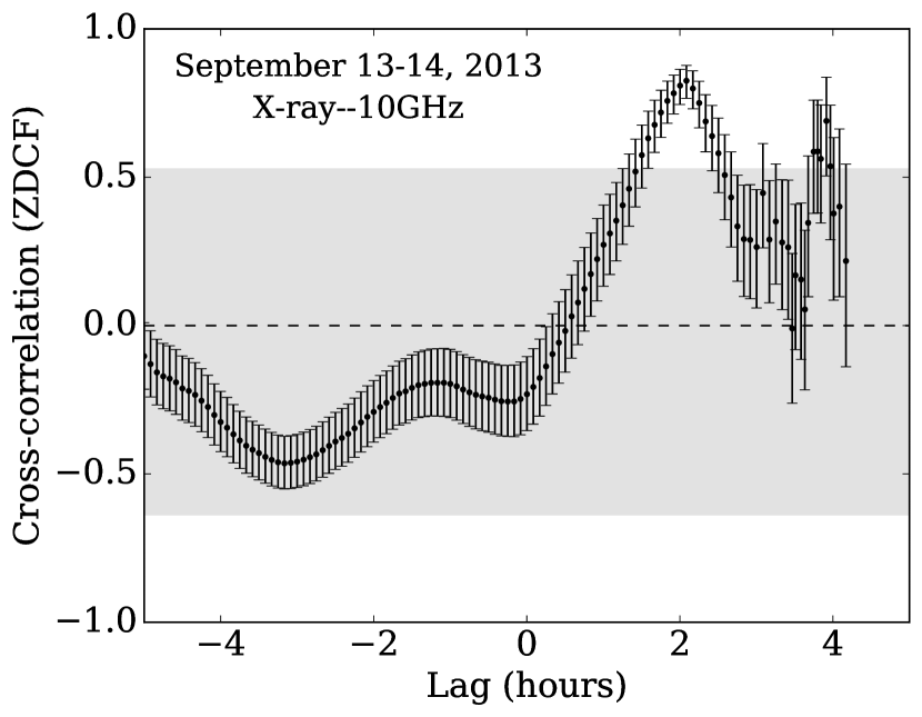
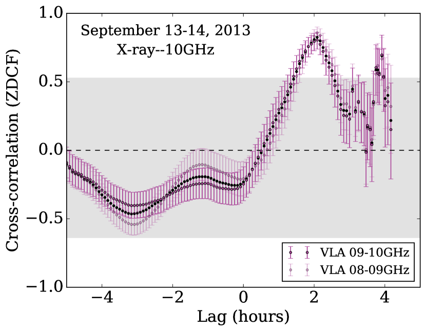
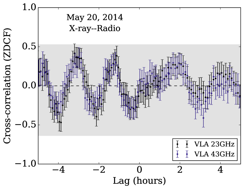
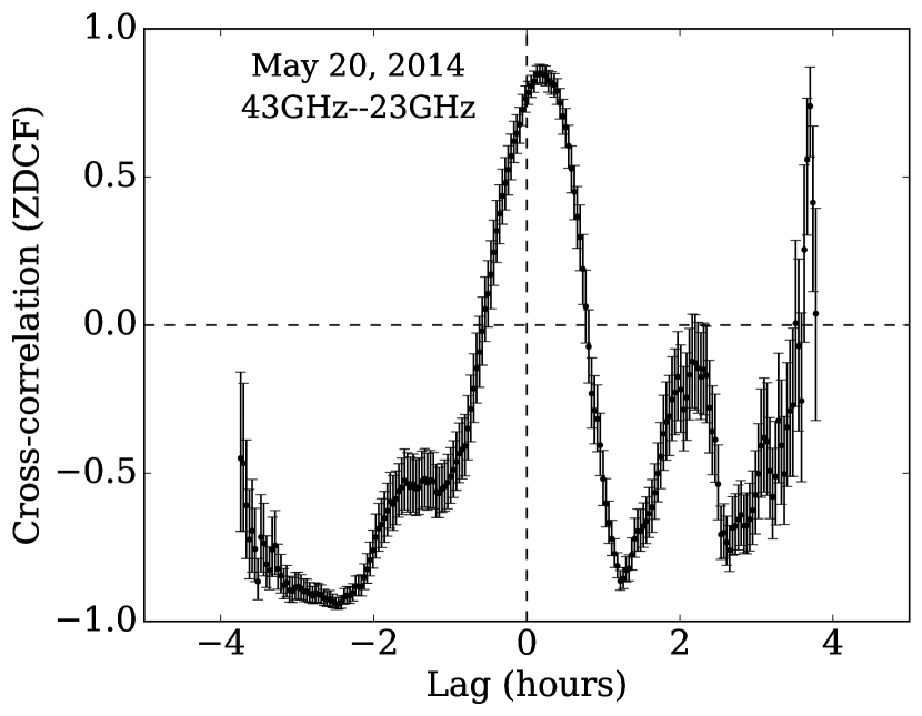
Figure 5: The ZDCF for the X-ray and radio light curves for 2013 September 14 (top panels) and for 2014 May 20 (bottom panels). The left panels are the cross-correlation between the X-ray and the average of all the radio spectral windows. The top right panel shows the cross-correlations between the X-ray and different radio frequency groupings. The bottom right panel shows the cross-correlation between two different JVLA frequency bands for 2014 May 20. A positive lag indicates structure appearing in the second data set (radio) after structure appears in the first (X-ray). The gray shaded regions denote the 2$\sigma$ error interval from the null hypothesis testing (see §6.1).

To quantify the lags between the peaks of potentially associated X-ray and radio variations, and assess the significance of the lags, we employ the $z$-transform discrete correlation function (ZDCF; Alexander, 1997). Unless otherwise noted, we calculate the X-ray–radio ZDCF using the average of all the radio spectral window groupings.

4.1 2013 July 27

Because of the poor calibration for this radio observation, particularly for the first half where the atmospheric phase stability was poor (see §3.2.1), we attempted to fit a smooth polynomial to the light curve before running the ZDCF. The ZDCF between the X-ray and radio does not return any significant features (see Fig. 6). Despite this, we can estimate an upper limit on the X-ray-to-radio time lag based on the center of the Bayesian Block flare detection in the X-ray and the start of the decline in the radio light curve during the second half of the radio observation, giving a time lag $\lesssim$80 min.

4.2 2013 September 14

The ZDCF for 2013 September 14 shows a strong peak, indicating a delay between the peaks of the X-ray and radio variability, with the X-ray peak leading by $\sim$125 minutes. The ZDCF is shown in the top left panel of Fig. 5. We also split the spectral windows in half and calculate the ZDCF using the higher- and lower-frequency spectral window groupings. Both spectral window groupings give the same strong peak in the ZDCF (top right panel Fig. 5).

However, the radio light curve of this observation continues to increase until the end of our temporal coverage, indicating that we may not be detecting the peak of the radio variability. This delay can thus be considered a lower limit on the time lag between the X-ray and radio, if they are indeed correlated (§6.1).

4.3 2013 October 28

Similar to the 2013 July 27 observation, we detect a decline in flux during the second half of the radio observation for 2013 October 28. In the X-ray, we detect two flares that precede the radio observation. The X-ray-to-radio ZDCF for the 2013 October 28 observation produces several peaks of low significance at $\sim$2, 4.25, and 7.5 hrs (see Fig. 6). We can also use the start of the decline of the radio flux density as an upper limit on the time of the peak of the potential radio flare, as we do for the 2013 July 27 observation, to obtain an upper limit on any time lag. If the radio variability is associated with the first X-ray flare, then the time lag between the X-ray and radio peaks is as high as $\sim$7.5 h, whereas if the detected radio emission is associated with the second flare, the lag is less than $\sim$3.9 h.

4.4 2014 May 20

Only very faint X-ray flares, if any, appear in the 2014 May 20 observation. Due to the low significance of a flare detection in the X-ray light curve (see §3.2.4), the ZDCF gives several minor peaks (bottom left panel of Fig. 5). In the light curves themselves, there appears to be a delay of $\sim$30 minutes between the peak flux in the X-ray and in the radio, with the X-ray leading the radio (bottom right panel of Fig. 1), as in the 2013 September 14 flare. The ZDCF instead appears to be identifying weak correlations between the radio variability at 8h to 9h UT and X-ray variability between 9h and 10h UT and between 11h and 12h UT.

5 Radio to Radio Cross-Correlation

For the analyses presented above, we have averaged over all frequencies for each radio observation. We also investigate the light curves for different frequency groupings for each observation. Generally, the light curve behavior is the same in each frequency grouping within a single VLA band, as shown for the K-band (18$-$26 GHz) observation on 2014 May 20 in the right panel of Fig. 3.

The 2013 September 14 radio data show some small differences at different frequencies, in particular, a drop in flux density and recovery in the lower frequency spectral windows (8$-$9 GHz) at the beginning of the observation. The peak of the radio variability also appears weaker at these lower frequencies. We checked the ZDCF for the X-ray to 8-9 GHz, compared to X-ray to 9-10 GHz, and they both show a strong peak in the same location (top right panel of Fig. 5).

2014 May 20 is the one observation in our sample with data in two different frequency bands (K-band, 23 GHz, and Q-band, 43 GHz). This is also one of the observations with clear structure in the radio light curve, allowing for comparisons between the light curves in the two different frequency windows. The lower-frequency, K-band light curve is already presented in Fig. 1. The higher-frequency, Q-band light curve is shown in the left panel of Fig. 4, along with the comparison source. To remove the structure in the light curve that is not intrinsic to SgrA*, we divide the SgrA* light curve by the comparison source (i.e., the phase calibrator, J1744$-$3116). For the purpose of comparing the two radio light curves, we do the same for the K-band light curve, and the two normalized light curves are presented in the right panel of Fig. 4.

We calculate the ZDCF for the two radio bands for the 2014 May 20 observation and find a delay between the Q-band (43 GHz) and K-band (23 GHz) of $\sim$10 minutes, with the higher-frequency light curve leading.

6 Discussion

6.1 Are the X-ray and Radio Correlated?

An important caveat to these results is that while X-ray flares tend to be distinct events that occur above a fairly smooth, constant background, the flux at longer wavelengths is almost constantly varying. The radio, in particular, shows variability at the 8%, 6%, and 10% level at 15, 23, and 43 GHz, respectively, on timescales $<$4 days (Macquart & Bower, 2006). Furthermore, Dexter & Fragile (2013) predict that Sgr A* has a tilted accretion disk and such a system could produce variability at millimeter wavelengths that is uncorrelated with shorter wavelength flaring.

To investigate whether the observed X-ray and radio variability is actually connected, we run a null hypothesis test to see, for example, if the radio variability in the 2013 September 14 light curve is connected to the bright X-ray flare, or if this could be a chance association of a bright X-ray flare with typical radio variability.

For this test, we utilize all of the X-ray and radio light curves that have substantial temporal overlap, which reduces our sample to seven observations. We subtract the UT start time of the radio from both the radio and X-ray light curves, so that all of the observations start at 0 UT. We then calculate the ZDCF for each pair of X-ray and radio light curves. The results are shown in Figure 6 — there is clear structure in the ZDCF even when the X-ray and radio light curves are mismatched. For example, the ZDCFs between the 2013 September 14 X-ray light curve and all of the radio light curves show structure similar to the ZDCF between the matched 2013 September 14 X-ray and radio light curves. This illustrates that the ZDCF alone does not prove a physical connection between apparently associated X-ray and radio variability.

Using the results of this test, we assess the significance of the ZDCF results presented earlier in Fig. 5. We combine the ZDCF values for all of the mismatched data (i.e., all of the off-diagonal panels in Fig. 6), and we calculate the 95.4th percentile ($\sim$2$\sigma$) in both the positive and negative direction. We identify these error intervals as gray shaded regions in Fig. 5. We note that the errors on the X-ray and radio time series are non-Gaussian, and thus the errors on the ZDCF may not be statistically correct. We present them here to provide intuition for the amplitude of the signal in the ZDCF for uncorrelated Sgr A* X-ray and radio data. Only the ZDCF for 2013 September 14 shows a cross-correlation peak outside of this error interval.

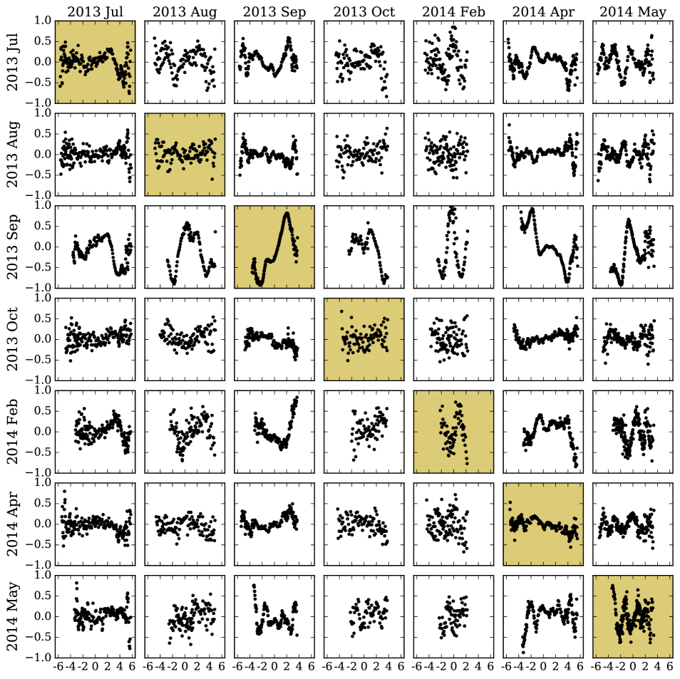
Figure 6: The ZDCFs for all pairs of X-ray and radio light curves presented in this paper. The panels along the diagonal, highlighted in yellow, show the correlations for the contemporaneous X-ray and radio observations, discussed in §4. The off-diagonal panels show the cross-correlation for mismatched X-ray–radio pairs. Although some of the contemporaneous cross-correlations (e.g., 2013 September 14) appear to be significant, many mismatched pairs of observations show comparable correlation peaks.

Another test for assessing the possible connection between X-ray and radio variability is to measure the typical radio variability and compare it to the radio variability during times of significant X-ray flaring. The strongest X-ray flare, observed on 2013 September 14, is accompanied by a rise of $\sim$15% over $\sim$176 min in the radio at 10 GHz. This is a larger rise on a much shorter time-scale than the $\sim$8% variability found by Macquart & Bower (2006) for a similar frequency (15 GHz). The light curve for 2014 April 28 (Fig. 1) at 10 GHz shows similar measurement errors, and has no clear X-ray flares during the X-ray observation, which begins $\sim$4 hr before and ends $\sim$2 hr after the radio observation. The 2014 April 28 radio light curve shows a steady decrease in flux of $\sim$4% over $\sim$6 hr, which is a much more gradual change than in the 2013 September 14 radio observation. These results make it less likely that this is a random radio fluctuation that happens to be contemporaneous with the X-ray flare. Another radio observation that may contain a counterpart to a weak X-ray flare, 2014 May 20, shows variability at the $\sim$9% level, which is right at the level of typical radio fluctuations from Macquart & Bower (2006), but again, this is over a time-scale of $\sim$90 min, which is much less than 4 days.

Future coordinated X-ray and radio campaigns, preferably at a single radio frequency, would help to establish whether the radio variability properties differ between times of significant X-ray flaring and times of X-ray quiescence.

Figure 7: The X-ray or NIR ($\lambda_{short}$) to sub-mm or radio ($\lambda_{long}$) time lags for reported flares in the literature and three flares reported in this work. The colored points correspond to X-ray flares, while the gray box and gray ‘x’ correspond to NIR-only flares. The references in the legend are Marrone et al. (2008, M08), Yusef-Zadeh et al. (2009, Y09), Eckart et al. (2012, E12), and Rauch et al. (2016, R16).

6.2 Comparisons to Previous Work

Obtaining simultaneous multiwavelength data of Sgr A* flares is challenging, and only a few previous observations of associated X-ray and submillimeter or radio flares exist. We collect all of the detections of presumably associated short- (X-ray and/or NIR) and long- (sub-mm and/or radio) wavelength flares from the literature, and plot the reported lags, along with our own detections, in Fig. 7. We assume that the short-wavelength flares (X-ray and IR) are simultaneous. However, there could be delays of a few to tens of minutes between the X-ray and IR, at least for fainter flares (Yusef-Zadeh et al., 2012, Fazio et al. in prep).

Marrone et al. (2008) and Yusef-Zadeh et al. (2008) report submillimeter and radio variability associated with simultaneous X-ray and IR flares on 2006 July 17. The peak in the submillimeter occurs $\sim$97 minutes after the X-ray peak (dark blue points in Fig. 7). Yusef-Zadeh et al. (2008) do not quantify the time lag between the X-ray or sub-mm and the radio, presumably because the radio peak could have occurred outside their temporal coverage.

Yusef-Zadeh et al. (2009), on the other hand, finds a delay of $\sim$315 minutes between an X-ray/NIR flare and a radio flare on 2007 April 4 (light blue point in Fig. 7), which is significantly longer than the delays we find here. Even though their radio coverage begins $\sim$3 hr after the X-ray/NIR flare ends, they argue that the radio flare is associated with the X-ray/NIR flare because of the high percentage flux increase compared to their other radio observations on different dates, the similar morphology between the X-ray and radio light curves, and the absence of a flare in the sub-mm (240 GHz) during the X-ray/NIR flaring event.

Eckart et al. (2012) present X-ray, NIR, sub-mm, and millimeter light curves of a flaring event on 2009 May 18, with the sub-mm and millimeter flares peaking about 45 and 75 minutes, respectively, after the simultaneous X-ray/NIR flares (green points in Fig. 7).

Mossoux et al. (2016) detect a rise in the radio at the same time as a flare in the X-ray and NIR on 2014 March 10. The radio observation ends just as the NIR flare is reaching its peak, however, and the authors attribute this rise in the radio to an X-ray/NIR flare that may have occurred before their observations began.

In addition to these few associated X-ray and sub-mm/radio flares, there are several reported cases in the literature of associated NIR and sub-mm flares. The delays between the NIR and sub-mm range from 90 to 200 minutes (Eckart et al., 2006, 2009; Yusef-Zadeh et al., 2006b; Marrone et al., 2008; Yusef-Zadeh et al., 2008, 2009; Eckart et al., 2008; Trap et al., 2011). There is one report of a lag of just 20 minutes between the NIR and sub-mm (Marrone et al., 2008), but Meyer et al. (2008) present additional NIR data showing that an NIR flare occurred just before the one presented in Marrone et al. (2008), giving a lag of 160 minutes. We present this general lag time of 90 to 200 minutes between the NIR and sub-mm as a gray box in Fig. 7.

On 2012 May 17, Rauch et al. (2016) detected an NIR flare, followed by a flare at 43GHz, with a lag of 270$\pm$30 minutes. As they lack X-ray information, we highlight this point with an ‘x’ in Fig. 7.

While the focus of our observing program is to look for correlations between X-ray and radio flaring activity, we have one observation with simultaneous observations in two different VLA radio bands (at 43 and 23 GHz). Yusef-Zadeh et al. (2006a) find a delay of 20 to 40 min and Brinkerink et al. (2015) find a delay of 28 $\pm$ 9 min between 43 and 22 GHz. We find a shorter time lag of $\sim$10 minutes between these two frequencies (see §5). Brinkerink et al. (2015) also finds a time lag of $\sim$20$-$40 min between submillimeter and different VLA bands. In these cases, the lower frequencies are delayed with respect to the higher frequencies, supporting the trends described above.

From Fig. 7, it is clear that there is not one typical lag time between shorter wavelength flares and sub-mm/radio variability. It is also clear that the associations between individual X-ray/NIR and radio flaring events is uncertain due to the lack of simultaneous data sampling long time-scales. However, as a whole, these results suggest that significant lags are common. If all flares had similar time lags, then one might expect a trend for increasing lag with wavelength, given the detected lags between sub-mm and radio frequencies (e.g., Brinkerink et al., 2015). Instead, there is considerable scatter, and while the longest lags have been found in the radio, they are not at the longest wavelengths. This may also support the scenario in which the reported correlations are spurious (§6.1).

For the X-ray$-$radio flares, the two flares with the longest delays, the 2007 April 4 flare from Yusef-Zadeh et al. (2009) and the 2013 September 14 flare from the current work, have peak X-ray count rates that exceed 1 count/s. These two are among the brightest X-ray flares known (e.g., Nowak et al., 2012; Ponti et al., 2015a, Haggard et al. in prep). Because our radio observations end during the flaring event on 2013 September 14, we do not know when the radio peak occurs, making it difficult to compare our time lag between the X-ray and radio with that measured by Yusef-Zadeh et al. (2009). The X-ray count rates for the two flares with lag times less than $\sim$80 min (bottom right in Fig. 7; $\sim$0.02$-$0.04 count/s) are much lower than for the flares with longer lags.

6.3 Comparisons to Flaring Models

There are many models in the literature that attempt to explain the flaring activity of Sgr A* at X-ray through radio wavelengths. Much of the focus is on the X-ray/NIR flares (and on synchrotron mechanisms), but several models attempt to explain the sub-mm and radio variations as well.

Dodds-Eden et al. (2010) present a model based on episodic magnetic reconnection near the last stable circular orbit of the super-massive black hole, followed by dissipation of magnetic energy. Their model includes energy loss via synchotron cooling and adiabatic expansion. The predicted light curves from their model show simultaneous flaring in the X-ray, NIR, and sub-mm, with a delayed peak in the radio. They argue that instead of “flares” occurring in the sub-mm and radio, there is a decrease in the sub-mm and radio flux during an X-ray/NIR flare, followed by a recovery. This recovery then appears as a flare, but is actually a return to quiescence. This model does not appear consistent with our X-ray–radio light curves. In particular, while the 2013 September 14 radio light curve shows a slight dip at the start of the X-ray flare, it then shows a significant rise in flux, well above the flux level in the radio prior to the X-ray flare.

Yusef-Zadeh et al. (2006a) adopt the plasmon model of van der Laan (1966) to explain the observed flaring activity. In this model, there is an adiabatically expanding “blob” of synchotron-emitting relativistic electrons that starts out optically thick at submillimeter and radio frequencies. Expansion of the blob’s surface area, while the blob remains optically thick, causes the initial rise of the flare. As the magnetic field decreases in strength, the electrons cool, and the column density of the expanding blob decreases, the blob becomes optically thin. At high frequencies, where the blob is initially optically thin, the model predicts simultaneous flaring and decline in emission. At lower frequencies, the flaring will be delayed, with the delay increasing with decreasing frequency. The predicted lags are consistent with the lags presented together in Fig. 7 and with the lags detected between different sub-mm and mm frequencies (e.g., Yusef-Zadeh et al., 2006a; Brinkerink et al., 2015).

Alternatively, if Sgr A* contains a jet (see, e.g., Falcke et al., 1993; Markoff et al., 2001), the expanding jet could also produce time lags between different sub-millimeter and radio frequencies (Yusef-Zadeh et al., 2006a; Falcke et al., 2009; Brinkerink et al., 2015; Rauch et al., 2016). The jet model can explain the IR to radio spectrum of Sgr A* (Falcke & Markoff, 2000; Mościbrodzka & Falcke, 2013; Mościbrodzka et al., 2014), and given the observed time lags, the jet should be at least mildly relativistic (Falcke et al., 2009).

General relativistic magnetohydrodynamic (GRMHD) simulations are also being used to explain Sgr A*’s multiwavelength variability and flaring. As mentioned in §6.1, Dexter & Fragile (2013) predict that Sgr A* has a tilted accretion disk, within which the emission is dominated by non-axisymmetric standing shocks from eccentric fluid orbits. From shock heating, multiple electron populations arise, producing the observed NIR emission from Sgr A*, which, in this model, is uncorrelated with longer wavelength emission. Alternatively, Chan et al. (2015) find that strong magnetic filaments, and their lensed images near the event horizon, can cause flaring in the IR and radio, with lags of about 60 minutes. However, their models produce no flaring in the X-ray, and the predicted lags are slightly smaller than the typical observed IR-to-submm/mm lags. Ball et al. (2016) include a population of non-thermal electrons located in highly magnetized regions (also previously considered by Yuan et al. 2003) and find that X-ray flares are a natural result. They find cases of simultaneous X-ray and IR flaring, as well as cases of IR flares with no X-ray counterparts, consistent with observational results. (e.g., Morris et al., 2012). However, Ball et al. (2016) do not comment on the emission at submm/mm wavelengths. The MHD model of Li et al. (2016) invokes magnetic reconnection, which leads to energetic electrons that then emit strong synchrotron radiation. Their model includes the ejections of plasma blobs, which then leads to the Yusef-Zadeh et al. (2006a) explanation of plasma blobs causing the frequency-dependent delays in observed flaring activity.

Despite intensive focus over the past $\sim$10 years, there is clearly more work to be done both on the modeling and the observational side of this problem. The time lags shown in Fig. 7, if real, indicate that not all flaring events have the same delay times between the X-ray/NIR and the sub-mm/mm peaks. This may indicate different physical properties of the plasma conditions for different events. Perhaps, if bright flares are caused by a magnetic reconnection event dissipating a large fraction of the magnetic field into an outflow, in the process accelerating particles to create a bright flare, there is less magnetic energy available to accelerate the fluid. Thus, the flow will be slower than if a smaller flare (or no flare) occurred, leading to a longer lag time for brighter flares than for weaker flares. In this work, we also detect an increase in the radio flux before the X-ray flare begins, which peaks after the X-ray emission returns to quiescence. In contrast, the X-ray/NIR and radio flares presented in Yusef-Zadeh et al. (2009) indicate a delay of the entire radio flare with respect to the X-ray/NIR flare, with the radio flare beginning long after the X-ray/NIR flare ends. More individual multiwavelength flare observations are required to build a consistent picture of the physics behind these events.

7 Conclusions

We report 9 contemporaneous Chandra X-ray and JVLA radio observations of Sgr A*, collected in 2013 and 2014. We detect a significant radio rise peaking $\gtrsim$176 min after the brightest X-ray flare ever detected from Sgr A* on 2013 September 14. We also detect a decline in radio flux in two observations (2013 July 27 and 2013 October 28), following weaker X-ray flares. Finally, we report a significant rise in radio flux at the same time as a tentative detection of a weak X-ray flare, with the radio peaking $\sim$30 min after the X-ray. We thus increase the number of X-ray–radio correlations from one to 5, where at least an upper or lower limit on the time lag between the two wavelength regimes can be measured (Table 2; Fig. 7).

Our study shows trends consistent with previous work on sub-millimeter and radio variability, which suggest a time lag between an X-ray and/or NIR peak and the sub-millimeter or radio counterpart (with the long wavelength data lagging the short wavelength rise). We also detect a time lag of $\sim$10 mins between the peaks of the 2014 May 20 radio variability at two different frequencies (43 and 22 GHz), again with the longer wavelength trailing the shorter wavelength. These results are generally consistent with either an expanding ‘blob’ or a jet, and combined with the other reported X-ray-to-radio lag in the literature, our results are suggestive of stronger X-ray flares leading to longer time lags in the radio.

However, the short durations ($\sim$5 hours) for the radio light curves makes it difficult to model Sgr A*’s overall radio variability and limits the utility of cross-correlation functions like the ZDCF. We perform a null hypothesis test to ascertain whether the correlations and time lags between the X-ray and radio variations are statistically significant. Cross-correlating mismatched X-ray and radio epochs give comparable correlations to the matched data. Hence, we find no statistical evidence that the X-ray flares and radio variability are correlated, though our results for the 2013 September 14 event remain suggestive. Further monitoring of Sgr A* in the X-ray and radio, and, in particular, characterizing the radio variability using non-parametric auto-correlation functions or parametrically, will be necessary to determine whether there is a physical connection between X-ray flaring and radio variability.

Appendix A Additional Radio Observations

In this Appendix, we include light curves for the observations where there was no clear flare in either the X-ray or the radio during the time of overlap between the two observations (see §3.2.5).

Figure 8: See caption for Fig. 1 for details.

References

- Alexander (1997) Alexander, T. 1997, in Astrophysics and Space Science Library, Vol. 218, Astronomical Time Series, ed. D. Maoz, A. Sternberg, & E. M. Leibowitz, 163
- Baganoff et al. (2001) Baganoff, F. K., Bautz, M. W., Brandt, W. N., et al. 2001, Nature, 413, 45
- Baganoff et al. (2003) Baganoff, F. K., Maeda, Y., Morris, M., et al. 2003, ApJ, 591, 891
- Ball et al. (2016) Ball, D., Özel, F., Psaltis, D., & Chan, C.-k. 2016, ApJ, 826, 77
- Boehle et al. (2016) Boehle, A., Ghez, A. M., Schödel, R., et al. 2016, ApJ, 830, 17
- Brinkerink et al. (2015) Brinkerink, C. D., Falcke, H., Law, C. J., et al. 2015, A&A, 576, A41
- Chan et al. (2015) Chan, C.-k., Psaltis, D., Özel, F., et al. 2015, ApJ, 812, 103
- Coti Zelati et al. (2015) Coti Zelati, F., Rea, N., Papitto, A., et al. 2015, MNRAS, 449, 2685
- Dexter & Fragile (2013) Dexter, J., & Fragile, P. C. 2013, MNRAS, 432, 2252
- Dodds-Eden et al. (2010) Dodds-Eden, K., Sharma, P., Quataert, E., et al. 2010, ApJ, 725, 450
- Dodds-Eden et al. (2009) Dodds-Eden, K., Porquet, D., Trap, G., et al. 2009, ApJ, 698, 676
- Eatough et al. (2013) Eatough, R. P., Falcke, H., Karuppusamy, R., et al. 2013, Nature, 501, 391
- Eckart et al. (2006) Eckart, A., Baganoff, F. K., Schödel, R., et al. 2006, A&A, 450, 535
- Eckart et al. (2008) Eckart, A., Schödel, R., García-Marín, M., et al. 2008, A&A, 492, 337
- Eckart et al. (2009) Eckart, A., Baganoff, F. K., Morris, M. R., et al. 2009, A&A, 500, 935
- Eckart et al. (2012) Eckart, A., García-Marín, M., Vogel, S. N., et al. 2012, A&A, 537, A52
- Falcke et al. (1993) Falcke, H., Mannheim, K., & Biermann, P. L. 1993, A&A, 278, L1
- Falcke & Markoff (2000) Falcke, H., & Markoff, S. 2000, A&A, 362, 113
- Falcke et al. (2009) Falcke, H., Markoff, S., & Bower, G. C. 2009, A&A, 496, 77
- Falcke & Markoff (2013) Falcke, H., & Markoff, S. B. 2013, Classical and Quantum Gravity, 30, 244003
- Fruscione et al. (2006) Fruscione, A., McDowell, J. C., Allen, G. E., et al. 2006, CIAO: Chandra’s data analysis system, , , doi:10.1117/12.671760
- Genzel et al. (2010) Genzel, R., Eisenhauer, F., & Gillessen, S. 2010, Reviews of Modern Physics, 82, 3121
- Ghez et al. (2008) Ghez, A. M., Salim, S., Weinberg, N. N., et al. 2008, ApJ, 689, 1044
- Gillessen et al. (2009) Gillessen, S., Eisenhauer, F., Fritz, T. K., et al. 2009, ApJ, 707, L114
- Gillessen et al. (2012) Gillessen, S., Genzel, R., Fritz, T., et al. 2012, Nature, 481, 51
- Gillessen et al. (2017) Gillessen, S., Plewa, P. M., Eisenhauer, F., et al. 2017, ApJ, 837, 30
- Ivezić et al. (2014) Ivezić, Ž., Connelly, A. J., VanderPlas, J. T., & Gray, A. 2014, Statistics, Data Mining, and Machine Learningin Astronomy
- Kennea et al. (2013) Kennea, J., Burrows, D., Kouveliotou, C., et al. 2013, The Astrophysical Journal Letters, 770, L24
- Li et al. (2016) Li, Y.-P., Yuan, F., & Wang, Q. D. 2016, ArXiv e-prints, arXiv:1611.02904
- Macquart & Bower (2006) Macquart, J.-P., & Bower, G. C. 2006, ApJ, 641, 302
- Markoff et al. (2001) Markoff, S., Falcke, H., Yuan, F., & Biermann, P. L. 2001, A&A, 379, L13
- Marrone et al. (2006) Marrone, D. P., Moran, J. M., Zhao, J.-H., & Rao, R. 2006, ApJ, 640, 308
- Marrone et al. (2008) Marrone, D. P., Baganoff, F. K., Morris, M. R., et al. 2008, ApJ, 682, 373
- McMullin et al. (2007) McMullin, J. P., Waters, B., Schiebel, D., Young, W., & Golap, K. 2007, in Astronomical Society of the Pacific Conference Series, Vol. 376, Astronomical Data Analysis Software and Systems XVI, ed. R. A. Shaw, F. Hill, & D. J. Bell, 127
- Meyer et al. (2008) Meyer, L., Do, T., Ghez, A., et al. 2008, ApJ, 688, L17
- Mori et al. (2013) Mori, K., Gotthelf, E. V., Zhang, S., et al. 2013, The Astrophysical Journal Letters, 770, L23
- Morris et al. (2012) Morris, M. R., Meyer, L., & Ghez, A. M. 2012, Research in Astronomy and Astrophysics, 12, 995
- Mościbrodzka & Falcke (2013) Mościbrodzka, M., & Falcke, H. 2013, A&A, 559, L3
- Mościbrodzka et al. (2014) Mościbrodzka, M., Falcke, H., Shiokawa, H., & Gammie, C. F. 2014, A&A, 570, A7
- Mossoux & Grosso (2017) Mossoux, E., & Grosso, N. 2017, ArXiv e-prints, arXiv:1704.08102
- Mossoux et al. (2015) Mossoux, E., Grosso, N., Vincent, F. H., & Porquet, D. 2015, A&A, 573, A46
- Mossoux et al. (2016) Mossoux, E., Grosso, N., Bushouse, H., et al. 2016, A&A, 589, A116
- Muno et al. (2009) Muno, M., Bauer, F., Baganoff, F., et al. 2009, The Astrophysical Journal Supplement Series, 181, 110
- Narayan et al. (1998) Narayan, R., Mahadevan, R., Grindlay, J. E., Popham, R. G., & Gammie, C. 1998, ApJ, 492, 554
- Neilsen et al. (2013) Neilsen, J., Nowak, M., Gammie, C., et al. 2013, The Astrophysical Journal, 774, 42
- Neilsen et al. (2015) Neilsen, J., Markoff, S., Nowak, M. A., et al. 2015, ApJ, 799, 199
- Nowak et al. (2012) Nowak, M., Neilsen, J., Markoff, S., et al. 2012, The Astrophysical Journal, 759, 95
- Pfuhl et al. (2015) Pfuhl, O., Gillessen, S., Eisenhauer, F., et al. 2015, The Astrophysical Journal, 798, 111
- Ponti et al. (2015a) Ponti, G., De Marco, B., Morris, M., et al. 2015a, Monthly Notices of the Royal Astronomical Society, 454, 1525
- Ponti et al. (2015b) Ponti, G., Bianchi, S., Muñoz-Darias, T., et al. 2015b, Monthly Notices of the Royal Astronomical Society, 446, 1536
- Ponti et al. (2017) Ponti, G., George, E., Scaringi, S., et al. 2017, MNRAS, 468, 2447
- Porquet et al. (2008) Porquet, D., Grosso, N., Predehl, P., et al. 2008, A&A, 488, 549
- Rauch et al. (2016) Rauch, C., Ros, E., Krichbaum, T. P., et al. 2016, A&A, 587, A37
- Rea et al. (2013) Rea, N., Esposito, P., Pons, J. A., et al. 2013, The Astrophysical Journal Letters, 775, L34
- Reid & Brunthaler (2004) Reid, M., & Brunthaler, A. 2004, The Astrophysical Journal, 616, 872
- Scargle (1998) Scargle, J. D. 1998, ApJ, 504, 405
- Scargle et al. (2013) Scargle, J. D., Norris, J. P., Jackson, B., & Chiang, J. 2013, ApJ, 764, 167
- Schödel et al. (2002) Schödel, R., Ott, T., Genzel, R., et al. 2002, Nature, 419, 694
- Shcherbakov et al. (2012) Shcherbakov, R. V., Penna, R. F., & McKinney, J. C. 2012, ApJ, 755, 133
- Trap et al. (2011) Trap, G., Goldwurm, A., Dodds-Eden, K., et al. 2011, A&A, 528, A140
- van der Laan (1966) van der Laan, H. 1966, Nature, 211, 1131
- Williams et al. (2017) Williams, P. K. G., Clavel, M., Newton, E., & Ryzhkov, D. 2017, pwkit: Astronomical utilities in Python, Astrophysics Source Code Library, , , ascl:1704.001
- Witzel et al. (2012) Witzel, G., Eckart, A., Bremer, M., et al. 2012, ApJS, 203, 18
- Witzel et al. (2014) Witzel, G., Ghez, A. M., Morris, M. R., et al. 2014, The Astrophysical Journal Letters, 796, L8
- Yuan et al. (2003) Yuan, F., Quataert, E., & Narayan, R. 2003, ApJ, 598, 301
- Yusef-Zadeh et al. (2015) Yusef-Zadeh, F., Bushouse, H., Schödel, R., et al. 2015, ApJ, 809, 10
- Yusef-Zadeh et al. (2006a) Yusef-Zadeh, F., Roberts, D., Wardle, M., Heinke, C. O., & Bower, G. C. 2006a, ApJ, 650, 189
- Yusef-Zadeh et al. (2008) Yusef-Zadeh, F., Wardle, M., Heinke, C., et al. 2008, ApJ, 682, 361
- Yusef-Zadeh et al. (2006b) Yusef-Zadeh, F., Bushouse, H., Dowell, C. D., et al. 2006b, ApJ, 644, 198
- Yusef-Zadeh et al. (2009) Yusef-Zadeh, F., Bushouse, H., Wardle, M., et al. 2009, ApJ, 706, 348
- Yusef-Zadeh et al. (2012) Yusef-Zadeh, F., Wardle, M., Dodds-Eden, K., et al. 2012, AJ, 144, 1