Object-Oriented Software for Functional Data

Abstract

This paper introduces the funData R package as an object-oriented implementation of functional data. It implements a unified framework for dense univariate and multivariate functional data on one- and higher dimensional domains as well as for irregular functional data. The aim of this package is to provide a user-friendly, self-contained core toolbox for functional data, including important functionalities for creating, accessing and modifying functional data objects, that can serve as a basis for other packages. The package further contains a full simulation toolbox, which is a useful feature when implementing and testing new methodological developments.

Based on the theory of object-oriented data analysis, it is shown why it is natural to implement functional data in an object-oriented manner. The classes and methods provided by funData are illustrated in many examples using two freely available datasets. The MFPCA package, which implements multivariate functional principal component analysis, is presented as an example for an advanced methodological package that uses the funData package as a basis, including a case study with real data. Both packages are publicly available on GitHub and CRAN.

1 Introduction

Functional data analysis is a branch of modern statistics that has seen a rapid growth in recent years. The technical progress in many fields of application allows to collect data in increasingly fine resolution, e.g., over time or space, such that the observed datapoints form quasi-continuous, possibly noisy, samples of smooth functions and are thus called functional data. One central aspect of functional data analysis is that the focus of the analysis is not a single data point, but the entirety of all datapoints that are considered to stem from the same curve. Researchers in functional data analysis have developed many new statistical methods for the analysis of this type of data, linking the concept of functional data also to related branches of statistics, such as the study of longitudinal data, which can be seen as sparse and often also irregular samples of smooth functions, or image data, that can be represented as functions on two-dimensional domains. New approaches focus on even more generalized functional objects (next generation functional data analysis, Wang et al., , 2016).

When it comes to the practical application of new methods to real data, appropriate software solutions are needed to represent functional data in an adequate manner and ideally in a way that new theoretical developments can be implemented easily. The most widely used R package for functional data is fda (Ramsay et al., , 2018), which is related to the popular textbook of Ramsay and Silverman, (2005). There are many other R packages for functional data that build on it, e.g., Funclustering (Soueidatt, , 2014), funFEM (Bouveyron, , 2015) or funHDDC (Schmutz et al., , 2018) or provide interfaces to fda, e.g., fda.usc (Febrero-Bande and Oviedo de la Fuente, , 2012) or refund (Goldsmith et al., , 2018). The fda package contains a class fd for representing dense functional data on one-dimensional domains together with many functionalities for fd objects, such as plotting or summaries. It implements a variety of functional data methods, for example principal component analysis, regression models or registration. The fd objects represent the data as a finite linear combination of given basis functions, such as splines or Fourier bases, i.e., they store the basis functions and the individual coefficients for each curve. This representation of course works best if the underlying function is smooth and can be represented well in the chosen basis. Moreover, the data should be observed with only a small degree of noise.

Alternatively to the basis function representation, the raw, observed data can be saved directly. There are two different approaches for organizing the observations: Many packages use matrices, that contain the data in a row-wise (e.g.,  fda.usc, refund) or column-wise (e.g., rainbow, Shang and Hyndman, (2016)) manner. This representation is most suitable for rather densely sampled data, where missing values can be coded via NA, which is supported by most of the packages. When it comes to irregular data, this way of storing functional data becomes quite inefficient, as the matrices then contain mostly missing values. Alternative solutions for sparse data or single points in 2D are list solutions (e.g., fdapace, Dai et al., (2018)) or data.frame based versions containing the data in a long format (e.g., fpca, Peng and Paul, (2011), fdaPDE, Lila et al., (2016) or sparseFLMM, Cederbaum, (2018)). Some packages also accept different formats (funcy, Yassouridis, (2018) or FDboost, Brockhaus and Ruegamer, (2018)).

Technically, realizations of functional data on one-dimensional domains can also be interpreted as multivariate time series. The CRAN taks view for time series analysis (https://CRAN.R-project.org/view=TimeSeries) lists a lot of packages for this type of data, among which the zoo package (Zeileis et al., , 2018; Zeileis and Grothendieck, , 2005) provides global infrastructure for regular and irregular time series. The main difference between functional data analysis and time series analysis is that for the former, each curve represents one observation of the same process, while for the latter the individual time points form the observations. Consequently, (multivariate) time series analysis aims more at analyzing the temporal dependence between curves and extrapolation/prediction of new time points, whereas the goal of functional data analysis is more in finding common structures between the curves (for example in PCA or clustering) and using them as predictors or response variables in regression models. More details on this topic can be found in the book of Ramsay and Silverman, (2005).

Image data, i.e., functions on two-dimensional domains are supported in refund, refund.wave (Huo et al., , 2014) and fdasrvf, (Tucker, , 2017). Some others, as e.g., fda and fda.usc implement image objects, but use them rather for representing covariance or coefficient surfaces from function-on-function regression than for storing data in form of images. The majority of the R packages for functional data, however, are restricted to single functions on one-dimensional domains. Methods for multivariate functional data, consisting of more than one function per observation unit, have also become relevant in recent years. The roahd package (Tarabelloni et al., , 2018) provides a special class for this type of data, while some others simply combine the data from the different functions in a list (e.g., fda.usc, Funclustering or RFgroove, Gregorutti, (2016)). For all of these packages, the elements of the multivariate functional data must be observed on one-dimensional domains, which means that combinations of functions and images for example are not supported. In addition, the one-dimensional observation grid must be the same for most of the implementations.

In summary, there exist already several software solutions for functional data, but there is still need for a unified, flexible representation of functional data, univariate and multivariate, on one- and higher dimensional domains and for dense and sparse functional data. The funData package (Happ, 2018a, ), which is in the main focus of this article, attempts to fill this gap. It provides a unified framework to represent all these different types of functional data together with utility methods for handling the data objects. In order to take account of the particular structure of functional data, the implementation is organized in an object-oriented manner. In this way, a link is established between the broad methodological field of object-oriented data analysis (Wang and Marron, , 2007), in which functional data analysis forms an important special case, and object-oriented programming (e.g., Meyer, , 1988), which is a fundamental concept in modern software engineering. It is shown why it is natural and reasonable to combine these two concepts for representing functional data.

In contrast to most R packages mentioned above, the funData package is not related to a certain type of methodology, such as regression, clustering or principal component analysis. Instead, it aims at providing a flexible and user-friendly core toolbox for functional data, which can serve as a basis for other packages, similarly to the Matrix package for linear algebra calculations for matrices (Bates and Maechler, , 2018). It further contains a complete simulation toolbox for generating functional data objects, which is fundamental for testing new functional data methods. The MFPCA package (Happ, 2018b, ), which is also presented in this article, is an example of a package that depends on funData. It implements a new methodological approach – multivariate functional principal component analysis for data on potentially different dimensional domains (Happ and Greven, , 2018) – that allows to calculate principal components and individual score values for e.g., functions and images, taking covariation between the elements into account. All implementation aspects that relate to functional data, i.e., input data, output data and all calculation steps involving functions are implemented using the object-oriented functionalities of the funData package. Both packages are publicly available on GitHub (https://github.com/ClaraHapp) and CRAN (https://CRAN.R-project.org).

The structure of this article is as follows: Section 2 contains a short introduction to the concept of object orientation in statistics and computer science and discusses how to adequately represent functional data in terms of software objects. The next section presents the object-oriented implementation of functional data in the funData package. Section 4 introduces the MFPCA package as an example on how to use the funData package for the implementation of new functional data methods. The final section contains a discussion and an outlook to potential future extensions.

2 Object orientation and functional data

Concepts of object orientation exist both in computer science and statistics. In statistics, the term object-oriented data analysis (OODA) has been introduced by Wang and Marron, (2007). They define it as “the statistical analysis of complex objects” and draw their attention on what they call the atom of the analysis. While in many parts of statistics these atoms are numbers or vectors (multivariate analysis), Wang and Marron, (2007) argue that they can be much more complex objects such as images, shapes, graphs or trees. Functional data analysis (Ramsay and Silverman, , 2005) is an important special case of object-oriented data analysis, where the atoms are functions. In most cases, they can be assumed to lie in $L^{2}(\mathcal{T})$, the space of square integrable functions on a domain $\mathcal{T}$. This space has infinite dimension, but being a Hilbert space, its mathematical structure has many parallels to the space ${\mathbb{R}}^{p}$ of $p$-dimensional vectors, which allows to transfer many concepts of multivariate statistics to the functional case in a quite straightforward manner.

In computer science, object orientation (Booch et al., , 2007; Armstrong, , 2006; Meyer, , 1988) is a programming paradigm which has profoundly changed the way how software is structured and developed. The key concept of object-oriented programming (OOP) is to replace the until then predominant procedural programs by computer programs made of objects, that can interact with each other and thus form, in a way, the “atoms” of the program. These objects usually consist of two blocks. First, a collection of data, which may have different data types, such as numbers, character strings or vectors of different length and is organized in fields. Second, a collection of methods, i.e., functions for accessing and/or modifying the data and for interacting with other objects. The entirety of all objects and their interactions forms the final program.

The main idea of the funData package is to combine the concepts of object orientation that exist in computer science and in statistics for the representation of functional data. The atom of the statistical analysis should thus be represented by the “atom” of the software program. The package therefore provides classes to organize the observed data in an appropriate manner. The class methods implement functionalities for accessing and modifying the data and for interaction between objects, which are primarily mathematical operations. The object orientation is realized in R via the S4 object system (Chambers, , 2008). This system fulfills most of the fundamental concepts of object-oriented programming listed in Armstrong, (2006) and is thus more rigorous than R’s widely used S3 system, which is used e.g., by fda or fda.usc. In particular, it checks for example if a given set of observation (time) points matches the observed data before constructing the functional data object.

For the theoretical analysis of functional data, the functions are mostly considered as elements of a function space such as $L^{2}(\mathcal{T})$. For the practical analysis, the data can of course only be obtained in finite resolution. Data with functional features therefore will always come in pairs of the form $(t_{ij},x_{ij})$ with

$$x_{ij}=x_{i}(t_{ij}),\quad j=1,\ldots,S_{i},\leavevmode\nobreak\ i=1,\ldots,N$$

for some functions $x_{1},\ldots,x_{N}$ that are considered as realizations of a random process $X:\mathcal{T}\to{\mathbb{R}}$. The domain $\mathcal{T}\subset{\mathbb{R}}^{d}$ here is assumed to be a compact set with finite (Lebesgue-) measure and in most cases, the dimension $d$ will be equal to $1$ (functions on one-dimensional domains), sometimes also $2$ (images) or $3$ (3D images). The observation points $t_{ij}\in\mathcal{T}$ in general can differ in their number and location between the individual functions.

When implementing functional data in an object-oriented way, it is thus natural to collect the data in two fields: the observation points $\{(t_{i1},\ldots,t_{iS_{i}})\colon\leavevmode\nobreak\ i=1,\ldots,N\}$ on one hand and the set of observed values $\{(x_{i1},\ldots,x_{iS_{i}})\colon\leavevmode\nobreak\ i=1,\ldots,N\}$ on the other hand. Both fields form the data block of the functional data object as an inseparable entity. This is a major advantage compared to non object-oriented implementations, that can consider the observation points and the observed values as parameters in their methods, but can not map the intrinsic dependence between both of them.

In the important special case that the functions are observed on a one-dimensional domain and that the arguments do not differ across functions, they can be collected in a single vector $(t_{1},\ldots,t_{S})$ and the observed values can be stored in a matrix $X$ with entries $x_{ij},\leavevmode\nobreak\ i=1,\ldots,N,\leavevmode\nobreak\ j=1,\ldots,S$. The matrix-based concept can be generalized to data observed on common grids on higher dimensional domains. In this case, the observation grid can be represented as a matrix (or array) or, in the case of a regular and rectangular grid, as a collection of vectors that define the marginals of the observation grid. The observed data is collected in an array with three or even higher dimensions.

In recent years, the study of multivariate functional data that takes multiple functions at the same time into account, has led to new insights. Each observation unit here consists of a fixed number of functions $p$, that can also differ in their domain (e.g., functions and images, Happ and Greven, , 2018). Technically, the observed values are assumed to stem from a random process $X=(X^{(1)},\ldots,X^{(p)})$, with random functions $X^{(k)}\colon\mathcal{T}_{k}\to{\mathbb{R}},\leavevmode\nobreak\ \mathcal{T}_{k}\in{\mathbb{R}}^{d_{k}},\leavevmode\nobreak\ k=1,\ldots,p$, that we call the elements of $X$. Realizations $x_{1},\ldots,x_{N}$ of such a process all have the same structure as $X$. If for example $p=2$ and $d_{1}=1,\leavevmode\nobreak\ d_{2}=2$, the realizations will all be bivariate functions with one functional and one image element. As data can only be obtained in finite resolution, observed multivariate functional data is of the form

$$(t_{ij}^{(k)},\leavevmode\nobreak\ x_{ij}^{(k)})\quad j=1,\ldots,S_{i}^{(k)},\leavevmode\nobreak\ i=1,\ldots,N,\leavevmode\nobreak\ k=1,\ldots,p.$$

Each element thus can be represented separately by its observation points and the observed values, and the full multivariate sample constitutes the collection of all the $p$ elements.

3 The funData package

The funData package implements the object-oriented approach for representing functional data in R. It provides three classes for functional data on one- and higher dimensional domains, multivariate functional data and irregularly sampled data, which are presented in Section 3.1. Section 3.2 presents the methods associated with the functional data classes based on two example datasets and Section 3.3 contains details on the integrated simulation toolbox.

3.1 Three classes for functional data

For the representation of functional data in terms of abstract classes – which, in turn, define concrete objects – we distinguish three different cases.

1. Class funData for dense functional data of “arbitrary” dimension (in most cases the dimension of the domain is $d\in\{1,2,3\}$) on a common set of observation points $t_{1},\ldots,t_{S}$ for all curves. The curves may have missing values coded by NA.

2. Class irregFunData for irregularly sampled functional data with individual sampling points $t_{ij},\leavevmode\nobreak\ j=1,\ldots,S_{i},\leavevmode\nobreak\ i=1,\ldots,N$ for all curves. The number $S_{i}$ and the location of observation points can vary across individual observations. At the moment, only data on one-dimensional domains is implemented.

3. Class multiFunData for multivariate functional data, which combines $p$ elements of functional data that may be defined on different dimensional domains (e.g., functions and images).

In the case of data on one-dimensional domains, the boundaries between the funData and the irregFunData class may of course be blurred in practice. The conceptual difference is that in 1. all curves are ideally supposed to be sampled on the full grid $T=\{t_{1},\ldots,t_{S}\}\subset\mathcal{T}$ and differences in the number of observation points per curve are mainly driven by anomalies or errors in the sampling process, such as missing values, which can be coded by NA. In contrast, case 2. a priori expects that the curves can be observed at different observation points $t_{ij}$, and that the number of observations per curve may vary.

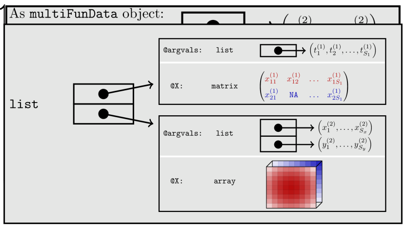
Figure 1: Left: An example of $N=3$ observations of functional data on a one-dimensional domain $\mathcal{T}$, observed on a common discrete grid $(t_{1},\ldots,t_{S})$, where the observed values $x_{ij}=x_{i}(t_{j})$ are represented by solid circles. The functions $x_{2}$ and $x_{3}$ have one missing value, each (open circles). Right: Representation of the data in a funData object. The @argvals slot is a list of length one, containing the observation grid as a vector. The @X slot is a matrix of dimension $N\times S$ that contains the observed values in row-wise format. Missing values are coded with NA.

Figure 2: Left: An example of $N=3$ observations of functional data on a two-dimensional domain $\mathcal{T}$. The functions are observed on a common discrete grid having $S_{x}$ points in $x$- and $S_{y}$ points in $y$-direction, i.e., each observation forms an image with $S_{x}\times S_{y}$ pixels. Right: Representation of the data in a funData object. The @argvals slot is a list of length $2$, containing the marginal sampling points. The slot @X is an array of dimension $N\times S_{x}\times S_{y}$.

For funData and irregFunData, the data is organized in two fields or slots, as they are called for S4 classes (Chambers, , 2008): The slot @argvals contains the observation points and the slot @X contains the observed data. For funData, the @argvals slot is a list, containing the common sampling grid for all functions and @X is an array containing all observations. In the simplest case of functions defined on a one-dimensional domain and sampled on a grid with $S$ observation points, @argvals is a list of length one, containing a vector of length $S$ and @X is a matrix of dimension $N\times S$, containing the observed values for each curve in a row-wise manner. For an illustration, see Figure 1. If the funData object is supposed to represent $N$ images with $S_{x}\times S_{y}$ pixels, @argvals is a list of length 2, containing two vectors with $S_{x}$ and $S_{y}$ entries, respectively, that represent the sampling grid. The slot @X is an array of dimension $N\times S_{x}\times S_{y}$, cf. Figure 2. For the irregFunData class, only functions on one-dimensional domains are currently implemented. The @argvals slot here is a list of length $N$, containing in its $i$-th entry the vector $(t_{i1},\ldots,t_{iS_{i}})$ with all observation points for the $i$-th curve. The @X slot organizes the observed values analogously, i.e., it is also a list of length $N$ with the $i$-th entry containing the vector $(x_{i1},\ldots,x_{iS_{i}})$. An illustration is given in Figure 3. The multiFunData class, finally, represents multivariate functional data with $p$ elements. An object of this class is simply a list of $p$ funData objects, representing the different elements. For an illustration, see Figure 4. Given specific data, the realizations of such classes are called funData, irregFunData or multiFunData objects. We will use the term functional data object in the following for referring to objects of all three classes.

Figure 3: Left: An example of $N=3$ irregular observations of functional data on a one-dimensional domain $\mathcal{T}$. The observation points for each function differ in number and location. Right: Representation of the data in an irregFunData object. Both the @argvals and the @X slot are a list of length $N$, containing the observation points $t_{ij}$ and the observed values $x_{ij}$.

Figure 4: Left: An example of $N=2$ observations of bivariate functional data on different domains, i.e., each observation (red/blue) consists of two elements, a curve and an image. Right: Representation of the data as a multiFunData object. As the data is bivariate, the multiFunData object is a list of length $2$, containing the two elements as funData objects.

3.2 Methods for functional data objects

Essential methods for functional data objects include for example the creation of an object from the observed data, methods for modifying and subsetting the data, plotting, arithmetics. The methods in the funData package are implemented such that they work on functional data objects as the atoms of the program, i.e., the methods accept functional data objects as input and/or have functional data objects as output. Moreover, all functions are implemented for the three different classes with appropriate sub-methods. This corresponds to the principle of polymorphism in Armstrong, (2006), as different classes have their own implementation e.g., of a plot function. In most cases, the methods for multiFunData objects will simply call the corresponding method for each element and concatenate the results appropriately.

3.2.1 Data used in the examples

The following code examples use the Canadian weather data (Ramsay and Silverman, , 2005), that is available e.g., in the fda package and the CD4 cell count data (Goldsmith et al., , 2013) from the refund package. In both cases, the data is observed on a one-dimensional domain. Examples for image data are included in the description of the simulation toolbox (Section 3.3).

The Canadian weather data contains daily and monthly observations of temperature (in °C) and precipitation (in mm) for $N=35$ Canadian weather stations, averaged over the years 1960 to 1994. We will use the daily temperature as an example for dense functional data on a one-dimensional domain. Moreover, it is combined with the monthly precipitation data to multivariate functional data with elements on different domains ($\mathcal{T}_{1}=[1,365]$ for the temperature and $\mathcal{T}_{2}=[1,12]$ for the precipitation).

The CD4 cell count data reports the number of CD4 cells per milliliter of blood for $N=366$ subjects who participated in a study on AIDS (MACS, Multicenter AIDS Cohort Study). CD4 cells are part of the human immune system and are attacked in the case of an infection with HIV. Their number thus can be interpreted as a proxy for the disease progression. For the present data, the CD4 counts were measured roughly twice a year and centered at the time of seroconversion, i.e., the time point when HIV becomes detectable. In total, the number of observations for each subject varies between $1$ and $11$ in the period of 18 months before and 42 months after seroconversion. The individual time points do also differ between subjects. The dataset thus serves as an example for irregular functional data. For more information on the data, please see Goldsmith et al., (2013).

3.2.2 Creating new objects and accessing an object’s information

The following code creates funData objects for the Canadian temperature and precipitation data:

R> data("CanadianWeather", package = "fda")

R> dailyTemp <- funData(argvals = 1:365,

+                       X = t(CanadianWeather$dailyAv[,, ’Temperature.C’]))

R> monthlyPrec <- funData(argvals = 1:12,

+                         X = t(CanadianWeather$monthlyPrecip))

It is then very easy to create a bivariate multiFunData object, containing the daily temperature and the monthly precipitation for the $35$ weather stations:

R> canadWeather <- multiFunData(dailyTemp, monthlyPrec)

The cd4 data in the refund package is stored in a matrix with $366\times 61$ entries, containing the CD4 counts for each patient on the common grid of all sampling points. Missing values are coded as NA. Since each patient has at least $1$ and at most $11$ observations, more than $90\%$ of the dataset consists of missings. Particularly, the time of seroconversion (time 0) is missing for all subjects. The irregFunData class stores only the observed values and their time points and is therefore more parsimonious. The following code extracts both separately as lists and then constructs an irregFunData object:

R> data("cd4", package = "refund")

R> allArgvals <- seq(-18, 42)

R> argvalsList <- apply(cd4, 1, function(x){allArgvals[complete.cases(x)]})

R> obsList <- apply(cd4, 1, function(x){x[complete.cases(x)]})

R> cd4Counts <- irregFunData(argvals = argvalsList, X = obsList)

When a functional data object is called in the command line, some basic information is printed to standard output. For the funData object containing the Canadian temperature data:

R> dailyTemp

Functional data with 35 observations of 1-dimensional support

argvals:

1 2 ... 365(365 sampling points)

X:

array of size 35 x 365

The multiFunData version lists the information of the different elements:

R> canadWeather

An object of class "multiFunData"

[[1]]

Functional data with 35 observations of 1-dimensional support

argvals:

1 2 ... 365(365 sampling points)

X:

array of size 35 x 365

[[2]]

Functional data with 35 observations of 1-dimensional support

argvals:

1 2 ... 12(12 sampling points)

X:

array of size 35 x 12

For irregFunData objects there is some additional information about the total number of observations. Note that time 0 has been dropped here, as there are no observations.

R> cd4Counts

Irregular functional data with 366 observations of 1-dimensional support

argvals:

Values in -18 ... 42.

X:

Values in 10 ... 3184.

Total:

1888 observations on 60 different argvals (1 - 11 per observation).

More information can be obtained using the usual summary or str functions:

R> summary(dailyTemp)

Argument values (@argvals):

         Min. 1st Qu. Median Mean 3rd Qu. Max.

Dim. 1 :    1      92    183  183     274  365

Observed functions (@X):

        St. Johns Halifax Sydney Yarmouth Charlottvl Fredericton

Min.        -7.00   -8.10  -8.40   -5.300    -10.400     -12.400

1st Qu.     -2.10   -2.60  -2.40   -0.100     -3.800      -4.700

Median       4.50    6.40   5.40    7.400      5.700       6.300

Mean         4.69    6.15   5.51    6.812      5.232       5.263

  ... [output truncated] ...

R> str(cd4Counts)

IrregFunData:

366 observations of 1-dimensional support on 60 different argvals (1 - 11 per curve).

@argvals: List of 366

 $ : int [1:3] -9 -3 3

 $ : int [1:4] -3 3 9 15

 $ : int [1:8] -15 -9 -3 3 9 17 22 29

  [list output truncated]

@X: List of 366

 $ : Named int [1:3] 548 893 657

  ..- attr(*, "names")= chr [1:3] "-9" "-3" "3"

 $ : Named int [1:4] 752 459 181 434

  ..- attr(*, "names")= chr [1:4] "-3" "3" "9" "15"

 $ : Named int [1:8] 846 1102 801 824 866 704 757 726

  ..- attr(*, "names")= chr [1:8] "-15" "-9" "-3" "3" ...

  [list output truncated]

The slots can be accessed directly via @argvals or @X. The preferable way of accessing and modifying the data in the slots, however, is via the usual get/set methods, following the principle of limited access (or encapsulation, Armstrong, , 2006), as an example:

R> argvals(monthlyPrec)

[[1]]

 [1]  1  2  3  4  5  6  7  8  9 10 11 12

The names can be set or get by the names function:

R> names(monthlyPrec) <- names(dailyTemp)

R> names(monthlyPrec)

 [1] "St. Johns"   "Halifax"     "Sydney"      "Yarmouth"    "Charlottvl"

 [6] "Fredericton" "Scheffervll" "Arvida"      "Bagottville" "Quebec"

[11] "Sherbrooke"  "Montreal"

 ... [output truncated] ...

The method nObs returns the number of observations (functions) in each object:

R> nObs(dailyTemp)

[1] 35

R> nObs(cd4Counts)

[1] 366

R> nObs(canadWeather)

[1] 35

The number of observation points is given by nObsPoints. Note that the functions in dailyTemp and canadWeather are densely sampled and therefore return a single number or two numbers (one for each element). For the irregularly sampled data in cd4Counts, the method returns a vector of length $N=366$, containing the individual number of observations for each subject:

R> nObsPoints(dailyTemp)

[1] 365

R> nObsPoints(cd4Counts)

 [1] 3 4 8 4 8 3 4 7 2 6 8 3

 ... [output truncated] ...

R> nObsPoints(canadWeather) # 365 (temp.) and 12 (prec.) observation points

[[1]]

[1] 365

[[2]]

[1] 12

The dimension of the domain can be obtained by the dimSupp method:

R> dimSupp(dailyTemp)

[1] 1

R> dimSupp(cd4Counts)

[1] 1

R> dimSupp(canadWeather) # both elements have one-dimensional support

[1] 1 1

Finally, a subset of the data can be extracted using R’s usual bracket notation or via the function extractObs (alias subset). We can for example extract the temperature data for the first five weather stations:

R> dailyTemp[1:5]

Functional data with 5 observations of 1-dimensional support

argvals:

1 2 ... 365(365 sampling points)

X:

array of size 5 x 365

or the CD4 counts of the first 8 patients before seroconversion (i.e., until time $0$):

R> extractObs(cd4Counts, obs = 1:8, argvals = -18:0)

Irregular functional data with 8 observations of 1-dimensional support

argvals:

Values in -17 ... -3.

X:

Values in 429 ... 1454.

Total:

15 observations on 6 different argvals (1 - 3 per observation).

In both cases, the method returns an object of the same class as the argument with which the function was called (funData for dailyTemp and irregFunData for cd4Counts), which is seen by the output.

3.2.3 Plotting

The more complex the data, the more important it is to have adequate visualization methods. The funData package comes with two plot methods for each class, one based on R’s standard plotting engine (plot.default and matplot) and one based on the ggplot2 implementation of the grammar of graphics (package ggplot2, Wickham, (2009); Wickham et al., (2018)). The plot function inherits all parameters from the plot.default function from the graphics package, i.e., colors, axis labels and many other options can be set as usual. The following code plots all 35 curves of the Canadian temperature data:

R> plot(dailyTemp, main = "Daily Temperature Data",

+       xlab = "Day of Year", ylab = "Temperature in °C")

and the CD4 counts of the first five patients on the log-scale:

R> plot(cd4Counts, obs = 1:5, xlim = c(-18, 45), log = "y",

+       main = "CD4 Counts for Individuals 1-5",

+       xlab = "Month since seroconversion",

+       ylab = "CD4 cell count (log-scale)")

R> legend("topright", legend = 1:5, col = rainbow(5), lty = 1, pch = 20,

+         title = "Individual")

For multivariate functional data, the different elements are plotted side by side, as shown here for the last ten Canadian weather stations:

R> plot(canadWeather, obs = 26:35, lwd = 2, log = c("", "y"),

+       main = c("Temperature", "Precipitation (log-scale)"),

+       xlab = c("Day of Year", "Month"),

+       ylab = c("Temperature in °C", "Precipitation in mm"))

The resulting plots are shown in Figure 5.

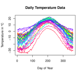
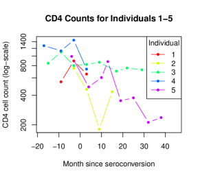
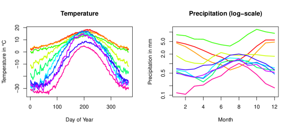
Figure 5: Results of the plot commands for functional data objects. First row: The daily temperature in $35$ Canadian weather stations (funData object, left) and the CD4 counts for the first five individuals (irregFunData object, right). Second row: The Canadian weather data for ten weather stations (multiFunData object). See text for the commands used; all other options were kept as defaults.

The optional autoplot / autolayer functions create a ggplot object that can be further modified by the user by loading the ggplot2 package and using the functionality provided therein. The following codes produce analogous plots to the plot examples above for the Canadian temperature data:

R> library("ggplot2")

R>

R> tempPlot <- autoplot(dailyTemp)

R> tempPlot + labs(title = "Daily Temperature Data",

+                  x = "Day of Year", y = "Temperature in °C")

and for the CD4 counts:

R> cd4Plot <- autoplot(cd4Counts, obs = 1:5)

R> cd4Plot + geom_line(aes(colour = obs)) +

+    labs(title = "CD4 Counts for Individuals 1-5", color = "Individual",

+       x = "Month since seroconversion", y = "CD4 cell count (log-scale)") +

+    scale_y_log10(breaks = seq(200,1000,200))

For the bivariate Canadian weather data, the bivariate plot is obtained via:

R> weatherPlot <- autoplot(canadWeather, obs = 26:35)

The subplots of the different elements can be customized separately, by changing for example the colors of the curves or adding axis labels, using functions from the ggplot2 package.

R> weatherPlot[[1]] <- weatherPlot[[1]] + geom_line(aes(colour = obs)) +

+    labs(title = "Temperature", colour = "Weather Station",

+         x = "Day of Year", y = "Temperature in °C")

R>

R> weatherPlot[[2]] <- weatherPlot[[2]] + geom_line(aes(colour = obs)) +

+    labs(title = "Precipitation (log-scale)", colour = "Weather Station",

+         x = "Month", y = "Precipitation in mm") +

+    scale_x_continuous(breaks = 1:12) +

+    scale_y_log10(breaks = c(0.1,0.5,1,5,10))

For the final plot, the subplots are arranged side by side using the gridExtra package (Auguie, , 2017):

R> gridExtra::grid.arrange(grobs = weatherPlot, nrow = 1)

The corresponding plots for all three data examples are shown in Figure 6.

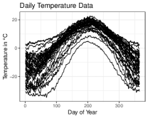
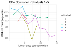
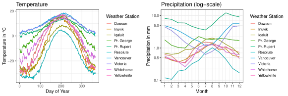
Figure 6: Results of the autoplot commands for functional data objects. First row: The daily temperature in $35$ Canadian weather stations (funData object, left) and the CD4 counts for the first five individuals (irregFunData object, right). Second row: The Canadian weather data for ten weather stations (multiFunData object). See text for the commands used. For all plots the option theme_bw() has been added for optimal print results; all other parameters were kept as defaults.

3.2.4 Coercion

As discussed earlier, there is no clear boundary between the irregFunData class and the funData class for functions on one-dimensional domains. The package thus provides coercion methods to convert funData objects to irregFunData objects, as seen in the output:

R> as.irregFunData(dailyTemp)

Irregular functional data with 35 observations of 1-dimensional support

argvals:

Values in 1 ... 365.

X:

Values in -34.8 ... 22.8.

Total:

12775 observations on 365 different argvals (365 - 365 per observation).

Vice versa the union of all observation points of all subjects is used as the common one and missing values are coded with NA (as.funData(cd4Counts)). Similarly, funData objects can also be coerced to multiFunData objects with only one element.

In order to simplify working with other R packages, functional data objects can be converted to a long data format via the function as.data.frame, here exemplarily shown for the CD4 count data:

R> as.data.frame(cd4Counts)

     obs argvals    X

1      1      -9  548

2      1      -3  893

3      1       3  657

4      2      -3  752

  ... [output truncated] ...

The funData package further provides coercion methods between funData objects and fd objects from package fda (funData2fd and fd2funData), which provides analysis tools for functional data and is also the basis of many other R packages.

3.2.5 Mathematical operations for functional data objects

With the funData package, mathematical operations can directly be applied to functional data objects, with the calculation made pointwise and the return being again an object of the same class. The operations build on the Arith and Math group generics for S4 classes. We can for example convert the Canadian temperature data from Celsius to Fahrenheit:

R> 9/5 * dailyTemp + 32

or calculate the logarithms of the CD4 count data:

R> log(cd4Counts)

Arithmetic operations such as sums or products are implemented for scalars and functional data objects as well as for two functional data objects. Note that in the last case, the functional data objects must have the same number of observations (in this case, the calculation is done with the $i$-th function of the first object and the $i$-th function of the second object) or one object may have only one observation (in this case, the calculation is made with each function of the other object). This is particularly useful e.g., for subtracting a common mean from all functions in an object, as in the following example, which uses the meanFunction method:

R> canadWeather - meanFunction(canadWeather)

Some of the demeaned curves are shown in Figure 7. Note that the functions also need to have the same observation points, which is especially important for irregFunData objects.

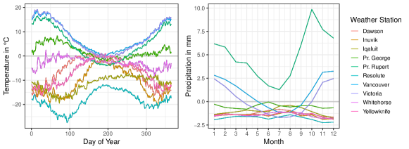
Figure 7: Demeaned versions of the ten canadianWeather observations shown in Figure 6. The curves have been obtained by canadWeather - meanFunction(canadWeather), i.e., the bivariate mean function of all $35$ weather stations has been subtracted from each observation. The horizontal gray lines mark zero, corresponding to the original mean function.

The tensorProduct function allows to calculate tensor products of functional data objects $f_{1},f_{2}$ on one-dimensional domains $\mathcal{T}_{1},\mathcal{T}_{2}$, respectively, i.e.,

$$f_{\text{Tens}}(t_{1},t_{2})=f_{1}(t_{1})f_{2}(t_{2})\quad t_{1}\in\mathcal{T}_{1},t_{2}\in\mathcal{T}_{2}.$$

The following code calculates the tensor product of the Canadian weather data and the output shows that the result is a funData object on a two-dimensional domain:

R> tensorData <- tensorProduct(dailyTemp, monthlyPrec)

R> tensorData

Functional data with 1225 observations of 2-dimensional support

argvals:

1 2 ... 365(365 sampling points)

1 2 ... 12(12 sampling points)

X:

array of size 1225 x 365 x 12

Two observations in tensorData are shown in Figure 8. Note that for image data, a single observation has to be specified for plotting.

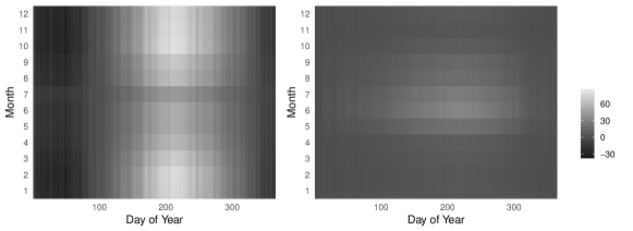
Figure 8: Two observations of the tensor product of daily temperature and monthly precipitation from the Canadian weather data, calculated via tensorProduct(dailyTemp, monthlyPrec). As seen in the plot, the domains of the functions have to be one-dimensional, but can be different. The result is an object of class funData on the two-dimensional domain $[1,356]\times[1,12]$ with $35^{2}=1225$ observations, from which two are shown here.

Another important aspect when working with functional data is integration, e.g., in the context of principal component analysis or regression, where scalar products between functions replace the usual scalar products between vectors from multivariate analysis. The funData package implements two quadrature rules, "midpoint" and "trapezoidal" (the default). The data is always integrated over the full domain and in the case of multivariate functional data, the integrals are calculated for each element and the results are added. For irregular data, the integral can be calculated on the observed points or they can be extrapolated linearly to the full domain. For the latter, curves with only one observation point are assumed to be constant.

Based on integrals, one defines the usual scalar product on $L^{2}(\mathcal{T})$ ${\langle f,g\rangle_{2}}=\int_{\mathcal{T}}f(t)g(t)\mathrm{d}t$ and the induced norm ${\left|\kern-1.07639pt\left|f\right|\kern-1.07639pt\right|_{2}}={\langle f,f\rangle_{2}}^{1/2}$ for $f,g\in L^{2}(\mathcal{T})$. For multivariate functional data on domains $\mathcal{T}_{1}\times\ldots\times\mathcal{T}_{p}$, the scalar product can be extended to

$$\langle\kern-1.07639pt\langle f,g\rangle\kern-1.07639pt\rangle=\sum_{j=1}^{p}f^{(j)}(t)g^{(j)}(t)\mathrm{d}t$$

with the induced norm ${\left|\kern-1.07639pt\left|\kern-1.07639pt\left|f\right|\kern-1.07639pt\right|\kern-1.07639pt\right|}=\langle\kern-1.07639pt\langle f,f\rangle\kern-1.07639pt\rangle^{1/2}$. The multivariate scalar product can further be generalized by introducing weights $w_{j}>0$ for each element (cf. Happ and Greven, , 2018):

$$\langle\kern-1.07639pt\langle f,g\rangle\kern-1.07639pt\rangle_{w}=\sum_{j=1}^{p}w_{j}{\langle f^{(j)},g^{(j)}\rangle_{2}}.$$ (1)

Scalar products and norms are implemented for all three classes in the funData package. Here also, the scalar product can be calculated for pairs of functions $f_{1},\ldots,f_{N}$ and $g_{1},\ldots,g_{N}$, hence ${\langle f_{i},g_{i}\rangle_{2}}$, or for a sample $f_{1},\ldots,f_{N}$ and a single function $g$, returning ${\langle f_{i},g\rangle_{2}}$. The norm function accepts some additional arguments, such as squared (logical, should the squared norm be calculated) or weight (a vector containing the weights $w_{1},\ldots,w_{p}$ for multivariate functional data):

R> all.equal(scalarProduct(dailyTemp, dailyTemp),

+            norm(dailyTemp, squared = TRUE))

[1] TRUE

3.3 Simulation toolbox

The funData package comes with a full simulation toolbox for univariate and multivariate functional data, which is a very useful feature when implementing and testing new methodological developments. The data is simulated based on a truncated Karhunen-Loève representation of functional data, as for example in the simulation studies in Scheipl and Greven, (2016) or Happ and Greven, (2018). All examples in the following text use set.seed(1) before calling a simulation function for reasons of reproducibility.

For univariate functions $x_{i}\colon\mathcal{T}\to{\mathbb{R}}$, the Karhunen-Loève representation of a function $x_{i}$ truncated at $M\in{\mathbb{N}}$ is given by

$$x_{i}(t)=\mu(t)+\sum_{m=1}^{M}\xi_{i,m}\phi_{m}(t),\quad i=1,\ldots,N,\leavevmode\nobreak\ t\in\mathcal{T}$$ (2)

with a common mean function $\mu(t)$ and principal component functions $\phi_{m},\leavevmode\nobreak\ m=1,\ldots,M$. The individual functional principal component scores $\xi_{i,m}={\langle x_{i},\phi_{m}\rangle_{2}}$ are realizations of random variables $\xi_{m}$ with ${\mathbb{E}}(\xi_{m})=0$ and $\operatorname{Var}(\xi_{m})=\lambda_{m}$ with eigenvalues $\lambda_{m}\geq 0$ that decrease towards $0$. This representation is valid for domains of arbitrary dimension, hence also for $\mathcal{T}\subset{\mathbb{R}}^{2}$ (images) or $\mathcal{T}\subset{\mathbb{R}}^{3}$ (3D images).

The simulation algorithm constructs new data from a system of $M$ orthonormal eigenfunctions $\phi_{1}\ldots\phi_{M}$ and scores $\xi_{i,m}$ according to the Karhunen-Loève representation Equation 2 with $\mu(t)\equiv 0$. For the eigenfunctions, the package implements Legendre polynomials, Fourier basis functions and eigenfunctions of the Wiener process including some variations (e.g., Fourier functions plus an orthogonalized version of the linear function). The scores are generated via

$$\xi_{i,m}\stackrel{{\scriptstyle\text{iid}}}{{\sim}}\operatorname{N}(0,\lambda_{m}),\leavevmode\nobreak\ m=1,\ldots,M,\leavevmode\nobreak\ i=1,\ldots,N.$$ (3)

For the eigenvalues $\lambda_{m}$, one can choose between a linear ($\lambda_{m}=\frac{M-m+1}{M}$) or exponential decrease ($\exp(-\tfrac{m+1}{2})$) or those of the Wiener process. New eigenfunctions and eigenvalues can be added to the package in an easy and modular manner.

The next code chunk simulates $N=8$ curves on the one-dimensional observation grid $\{0,0.01,0.02,\ldots,1\}$ based on the first $M=10$ Fourier basis functions on $[0,1]$ and eigenvalues with a linear decrease:

R> simUniv1D <- simFunData(N = 8, argvals = seq(0,1,0.01),

+                          eFunType = "Fourier", eValType = "linear", M = 10)

The function returns a list with $3$ entries: The simulated data (simData, a funData object shown in Figure 9), the true eigenvalues (trueVals) and eigenfunctions (trueFuns, also as a funData object).

For simulating functional data on a two- or higher dimensional domain, simFunData constructs eigenfunctions based on tensor products of univariate eigenfunctions. The user thus has to supply the parameters that relate to the eigenfunctions as a list (for argvals) or as a vector (M and eFunType), containing the information for each marginal. The total number of eigenfunctions equals to the product of the entries of $M$. The following example code simulates $N=5$ functions on $\mathcal{T}=[0,1]\times[-0.5,0.5]$. The eigenfunctions are calculated as tensor products of $M_{1}=10$ eigenfunctions of the Wiener process on $[0,1]$ and $M_{2}=12$ Fourier basis functions on $[-0.5,0.5]$. In total, this leads to $M=M_{1}\cdot M_{2}=120$ eigenfunctions. For each eigenfunction and each observed curve, the scores $\xi_{i,m}$ are generated as in Equation 3 with linearly decreasing eigenvalues:

R> argvalsList <- list(seq(0,1,0.01), seq(-0.5,0.5, 0.01))

R> simUniv2D <- simFunData(N = 5, argvals = argvalsList,

+       eFunType = c("Wiener", "Fourier"), eValType = "linear", M = c(10,12))

The first simulated image is shown in Figure 9. As for functions on one-dimensional domains, the function returns the simulated data together with the true eigenvalues and eigenfunctions.

For multivariate functional data, the simulation is based on the multivariate version of the Karhunen-Loève Theorem (Happ and Greven, , 2018) for multivariate functional data $x_{i}=(x_{i}^{(1)},\ldots,x_{i}^{(p)})$ truncated at $M\in{\mathbb{N}}$

$$x_{i}(t)=\mu(t)+\sum_{m=1}^{M}\rho_{i,m}\psi_{m}(t),\quad i=1,\ldots,N,\leavevmode\nobreak\ t=(t_{1},\ldots,t_{p})\in\mathcal{T}_{1}\times\ldots\times\mathcal{T}_{p}$$ (4)

with a multivariate mean function $\mu$ and multivariate eigenfunctions $\psi_{m}$ that have the same structure as $x_{i}$ (i.e., if $x_{i}$ consists of a function and an image, then $\mu$ and $\psi_{m}$ will also be bivariate functions, consisting of a function and an image). The individual scores $\rho_{i,m}=\langle\kern-1.07639pt\langle x_{i},\psi_{m}\rangle\kern-1.07639pt\rangle$ for each observation $x_{i}$ and each eigenfunction $\psi_{m}$ are real numbers and have the same properties as in the univariate case, i.e., they are realizations of random variables $\rho_{m}$ with ${\mathbb{E}}(\rho_{m})=0$ and $\operatorname{Var}(\rho_{m})=\nu_{m}$ with eigenvalues $\nu_{m}\geq 0$ that again form a decreasing sequence that converges towards $0$. As in the univariate case, the multivariate functions are simulated based on eigenfunctions and scores according to Equation 4 with $\mu(t)\equiv 0$. The scores are sampled independently from a $\operatorname{N}(0,\nu_{m})$ distribution with decreasing eigenvalues $\nu_{m}$, analogously to Equation 3. For the construction of multivariate eigenfunctions, Happ and Greven, (2018) propose two approaches based on univariate orthonormal systems, which are both implemented in the simMultiFunData function.

Calling simMultiFunData with the option "split" constructs multivariate eigenfunctions by splitting orthonormal functions into $p$ pieces and shifting them to where the elements should be defined. This works only for functions on one-dimensional domains. The following code simulates $N=7$ bivariate functions on $[-0.5,0.5]$ and $[0,1]$, based on $M=10$ Fourier basis functions and linearly decreasing eigenvalues.

R> argvalsList <- list(seq(-0.5,0.5,0.01), seq(0,1,0.01))

R> simMultiSplit <- simMultiFunData(N = 7, argvals = argvalsList,

+                      eFunType = "Fourier", eValType = "linear", M = 10,

+                      type = "split")

As an alternative, multivariate eigenfunctions can be constructed as weighted versions of univariate eigenfunctions. With this approach, one can also simulate multivariate functional data on different dimensional domains, e.g., functions and images. It is implemented in funData’s simMultiFunData method using the option type = "weighted". The following code simulates $N=5$ bivariate functions on $\mathcal{T}_{1}=[-0.5,0.5]$ and $\mathcal{T}_{2}=[0,1]\times[-1,1]$. The first elements of the eigenfunctions are derived from $M_{1}=12$ Fourier basis functions on $\mathcal{T}_{1}$ and the second elements of the eigenfunctions are constructed from tensor products of $4$ eigenfunctions of the Wiener process on $[0,1]$ and $3$ Legendre polynomials on $[-1,1]$, which give together $M_{2}=12$ eigenfunctions on $\mathcal{T}_{2}$. The scores are sampled using exponentially decreasing eigenvalues:

R> argvalsList <- list(seq(-0.5,0.5,0.01), list(seq(0,1,0.01), seq(-1,1,0.01)))

R> simMultiWeight <- simMultiFunData(N = 5, argvals = argvalsList,

+                       eFunType = list("Fourier", c("Wiener", "Poly")),

+                       eValType = "exponential",  M = list(12, c(4,3)),

+                       type = "weighted")

In both cases, the result contains the simulated data as well as the eigenfunctions and eigenvalues. The simulated functions are shown in Figures 10 and 11. For more technical details on the construction of the eigenfunctions, see Happ and Greven, (2018).

Once simulated, the data can be further processed by adding noise (function addError) or by artificially deleting measurements (sparsification, function sparsify). The latter is done in analogy to Yao et al., (2005). Examples for modified versions of simulated functions can be computed as follows:

R> addError(simUniv1D$simData, sd = 0.5)

R> sparsify(simUniv1D$simData, minObs = 5, maxObs = 10)

R>

R> addError(simMultiWeight$simData, sd = c(0.5, 0.3))

R> sparsify(simMultiSplit$simData, minObs = c(5, 50), maxObs = c(10, 80))

The results are shown in Figure 12 for the univariate case and in Figure 13 for the multivariate case.

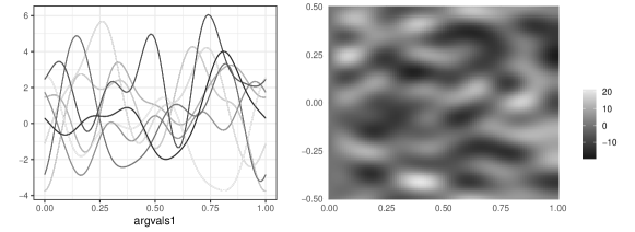
Figure 9: Left: $N=8$ simulated curves on $[0,1]$ based on the first $M=10$ Fourier basis functions and eigenvalues with a linear decrease. Right: One simulated image on $[0,1]\times[-0.5,0.5]$ based on tensor products of $M_{1}=10$ eigenfunctions of the Wiener process on $[0,1]$ and $M_{2}=12$ Fourier basis functions on $[-0.5,0.5]$ and linearly decreasing eigenvalues.

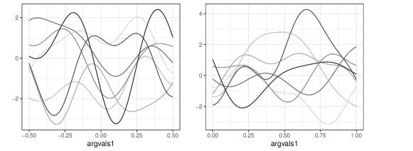
Figure 10: $N=7$ simulated bivariate curves on $[-0.5,0.5]$ and $[0,1]$ with eigenfunctions obtained from the first $M=10$ Fourier basis functions by the splitting algorithm (type = "split") and linearly decreasing eigenvalues.

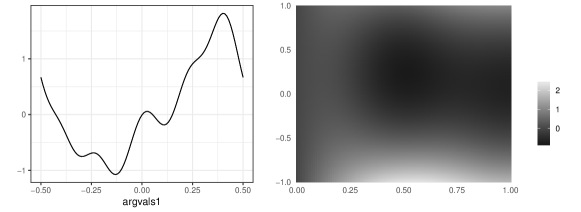
Figure 11: One observation of simulated bivariate data on $[-0.5,0.5]$ and $[0,1]\times[-1,1]$ using weighted orthonormal elements (type = "weighted"). See text for details.

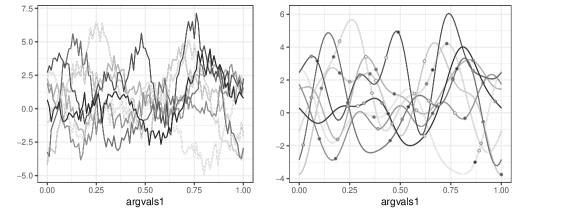
Figure 12: Transforming the simulated univariate functions in simUniv1D (see Figure 9). Left: Adding noise with a standard deviation of $\sigma=0.5$. Right: The effect of sparsification, keeping five to ten observations per curve. Solid lines show the original data, filled dots correspond to the observed values of the sparsified version.

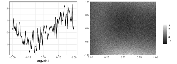
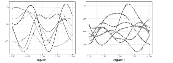
Figure 13: Transforming the simulated bivariate data. First row: A noisy version of the first observation of simMultiWeight (see Figure 11). Second row: All $7$ observations of simMultiSplit after sparsification (see Figure 10). Solid lines show the original data, filled dots correspond to the observed values of the sparsified version. Note that the standard deviation in the noise as well as the degree of sparsification varies across elements.

4 The MFPCA package

The MFPCA package implements multivariate functional principal component analysis (MFPCA) for data on potentially different dimensional domains (Happ and Greven, , 2018). It heavily builds upon the funData package, i.e., all functions are implemented as functional data objects. The MFPCA package thus illustrates the use of funData as a universal basis for implementing new methods for functional data. Section 4.1 gives a short review of the MFPCA methodology and Section 4.2 describes the implementation including a detailed description of the main functions and a practical case study. For theoretical details, please refer to Happ and Greven, (2018).

4.1 Methodological background

The basic idea of MFPCA is to extend functional principal component analysis to multivariate functional data on different dimensional domains. The data is assumed to be iid samples $x_{1},\ldots,x_{N}$ of a random process $X=(X^{(1)},\ldots,X^{(p)})$ with $p$ elements $X^{(j)}\in L^{2}(\mathcal{T}_{j})$ on domains $\mathcal{T}_{j}\subset{\mathbb{R}}^{d_{j}}$ with potentially different dimensional dimensions $d_{j}\in{\mathbb{N}}$. Happ and Greven, (2018) provide an algorithm to estimate multivariate functional principal components and scores based on their univariate counterparts. The algorithm starts with demeaned samples $x_{1},\ldots,x_{N}$ and consists of four steps:

1. Calculate a univariate functional principal component analysis for each element $j=1,\ldots,p$. This results in principal component functions $\hat{\phi}_{1}^{(j)},\ldots,\hat{\phi}_{M_{j}}^{(j)}$ and principal component scores $\hat{\xi}_{i,1}^{(j)},\ldots,\hat{\xi}_{i,M_{j}}^{(j)}$ for each observation unit $i=1,\ldots,N$ and suitably chosen truncation lags $M_{j}$.

2. Combine all coefficients into one big matrix $\Xi\in{\mathbb{R}}^{N\times M_{+}}$ with $M_{+}=M_{1}+\ldots+M_{p}$, having rows

   $$\Xi_{i,\cdot}=\left(\hat{\xi}_{i,1}^{(1)},\ldots,\hat{\xi}_{i,M_{1}}^{(1)},\ldots,\hat{\xi}_{i,1}^{(p)},\ldots,\hat{\xi}_{i,M_{p}}^{(p)}\right)$$

   and estimate the joint covariance matrix $\hat{Z}=\frac{1}{N-1}\Xi^{\top}\Xi$.

3. Find eigenvectors $\hat{c}_{m}$ and eigenvalues $\hat{\nu}_{m}$ of $\hat{Z}$ for $m=1,\ldots,M$ for some truncation lag $M\leq M_{+}$.

4. Calculate estimated multivariate principal component functions $\hat{\psi}_{m}$ and scores $\hat{\rho}_{i,m}$ based on the results from steps 1 and 3:

   $$\hat{\psi}_{m}^{(j)}=\sum_{n=1}^{M_{j}}[\hat{c}_{m}]_{n}^{(j)}\hat{\phi}_{n}^{(j)},\qquad\hat{\rho}_{i,m}=\sum_{j=1}^{p}\sum_{n=1}^{M_{j}}[\hat{c}_{m}]_{n}^{(j)}\hat{\xi}_{i,n}^{(j)}=\Xi_{i,\cdot}\hat{c}_{m},\quad m=1,\ldots,M.$$

The advantage of MFPCA with respect to univariate FPCA for each component can be seen in steps 2 and 3: The multivariate version takes covariation between the different elements into account, by using the joint covariance of the scores of all elements.

As discussed for the simulation in Section 3.3, the multivariate principal component functions will have the same structure as the original samples, i.e., $\hat{\psi}_{m}=\left(\hat{\psi}_{m}^{(1)},\ldots,\hat{\psi}_{m}^{(p)}\right)$ with $\hat{\psi}_{m}^{(j)}\in L^{2}(\mathcal{T}_{j})$ for $m=1,\ldots,M$. The scores $\hat{\rho}_{i,m}$ give the individual weight of each observation $x_{i}$ for the principal component $\hat{\psi}_{m}$ in the empirical version of the truncated multivariate Karhunen-Loève representation:

$$x_{i}\approx\hat{\mu}+\sum_{m=1}^{M}\hat{\rho}_{i,m}\hat{\psi}_{m},$$ (5)

with $\hat{\mu}$ being an estimate for the multivariate mean function, cf. Equation 4.

In some cases, it might be of interest to replace the univariate functional principal component analysis in step 1 by a representation in terms of fixed basis functions $B_{1}^{(j)},\ldots,B_{K_{j}}^{(j)}$, such as splines. In Happ and Greven, (2018) it is shown how the algorithm can be extended to arbitrary basis functions in $L^{2}(\mathcal{T}_{j})$. Mixed approaches with some elements expanded in principal components and others for instance in splines are also possible. Another very likely case is that the elements of the multivariate functional data differ in their domain, range or variation. For this case, Happ and Greven, (2018) develop a weighted version of MFPCA with weights $w_{j}>0$ for the different elements $j=1,\ldots,p$. The weights have to be chosen depending on the data and the question of interest. One possible choice is to use the inverse of the integrated pointwise variance for the weights, as proposed in Happ and Greven, (2018): $w_{j}=\left(\int_{\mathcal{T}_{j}}\widehat{\operatorname{Var}}(X^{(j)}(t))\mathrm{d}t\right)^{-1}$.

4.2 MFPCA implementation

The main function in the MFPCA package is MFPCA, that calculates the multivariate functional principal component analysis. It requires as input arguments a multiFunData object for which the MFPCA should be calculated, the number of principal components M to calculate and a list uniExpansions specifying the univariate representations to use in step 1. It returns an object of class MFPCAfit, which has methods for printing, plotting and summarizing. Before discussing the detailed options, we illustrate the usage of MFPCA with a real data application.

4.2.1 Case study: Calculating the MFPCA for the Canadian weather data

The following example calculates a multivariate functional principal component analysis for the bivariate Canadian weather data with three principal components, using univariate FPCA with five principal components for the daily temperature (element 1) and univariate FPCA with four principal components for the monthly precipitation (element 2). The univariate expansions are specified in a list with two list entries (one for each element) and are then passed to the main function:

R> uniExpansions <- list(list(type = "uFPCA", npc = 5), # temperature element

+                      list(type = "uFPCA", npc = 4)) # precipitation element

R> MFPCAweather <- MFPCA(canadWeather, M = 3, uniExpansions = uniExpansions)

The full analysis takes roughly nine seconds on a standard laptop, with most time spent for the univariate decompositions (if the elements are for example expanded in penalized splines, the total calculation time reduces to one second).

The resulting object MFPCAweather contains the following elements: the multivariate mean function (meanFunction, as the data is demeaned automatically before the analysis), the empirical multivariate principal component functions (functions), the individual scores for each city (scores) and the estimated eigenvalues (values). Two additional elements can be used for calculating out-of-sample predictions (vectors and normFactors). The summary function gives a basic overview of the results.

R> summary(MFPCAweather)

3 multivariate functional principal components estimated with 2 elements, each.

                     * * * * * * * * * *

                                     PC 1     PC 2     PC 3

Eigenvalue                       1.55e+04 1.48e+03 3.30e+02

Proportion of variance explained 8.96e-01 8.54e-02 1.90e-02

Cumulative proportion            8.96e-01 9.81e-01 1.00e+00

The eigenvalues here are rapidly decreasing, i.e., the first principal component already explains almost $90\%$ of the variability in the data. The decrease of the eigenvalues is graphically illustrated by the screeplot function (see Figure 17 in the appendix).

All functions in MFPCAweather are represented as functional data objects and can thus be plotted using the methods provided by the funData package (see Figure 14). The mean function of the temperature element is seen to have low values below -10°C in the winter and a peak at around 15°C in the summer, while the mean of the monthly precipitation data is slightly increasing over the year. The first principal component is negative for both elements, i.e., weather stations with positive scores will in general have lower temperatures and less precipitation than on average. The difference is more pronounced in the winter than in the summer, as both the temperature as well as the precipitation element of the first principal component have more negative values in the winter period. This indicates that there is covariation between both elements, that can be captured by the MFPCA approach. An alternative visualization, plotting the principal component as perturbation of the mean as in the fda package, can be obtained via plot(MFPCAweather) (see Figure 18 in the appendix). In total, the first bivariate eigenfunction can be associated with arctic and continental climate, characterized by low temperatures, especially in the winter, and less precipitation than on average. Weather stations with negative score values will show an opposite behavior, with higher temperatures and more rainfall than on average, particularly in the winter months. This is typical for maritime climate.

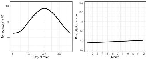
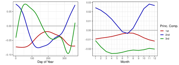
Figure 14: MFPCA results for the Canadian weather data. First row: The bivariate mean function, which is subtracted from the data before calculating the MFPCA. Second row: The first three bivariate functional principal components. The gray horizontal lines in the principal component plots mark zero.

The estimated scores for the first principal component support this interpretation, as weather stations in arctic and continental areas mainly have positive scores, while stations in the coastal areas have negative values in most cases (see Figure 15). Moreover, weather stations in the arctic and pacific regions are seen to have more extreme score values than those in continental areas and on the Atlantic coast, meaning that the latter have a more moderate climate. An alternative visualization of the scores is given by the scoreplot function (see Figure 19 in the appendix).

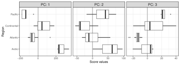
Figure 15: Scores of the first three bivariate functional principal components (PCs) for the Canadian weather data depending on the region of each weather station. The gray vertical lines mark zero.

4.2.2 More details on the MFPCA function

In the above example, both univariate elements have been decomposed in univariate functional principal components in step 1. The MFPCA package implements some further options for the univariate expansions, that can easily be extended in a modular way. The most common basis expansions are uFPCA (univariate PCA) and splines1D / splines1Dpen (splines) for elements on a one-dimensional domain and splines2D / splines2Dpen (tensor splines) and DCT2D/DCT3D (tensor cosine basis) for elements on higher dimensional domains. If data has been smoothed, for example in a preprocessing step, the basis functions and coefficients can also be passed using type = "given" for the univariate basis expansions. All currently implemented basis expansions are presented in detail in the appendix.

With the mean function, the principal components and the individual scores calculated in the MFPCA function, the observed functions $x_{1},\ldots,x_{N}$ can be reconstructed based on the truncated Karhunen-Loève representation with plugged-in estimators as in Equation 5. The reconstructions can be obtained by setting the option fit = TRUE, which adds a multivariate functional data object fit with $N$ observations to the result object, where the $i$-th entry corresponds to the reconstruction $\hat{x}_{i}$ of an observation $x_{i}$. For a weighted version of MFPCA, the weights can be supplied to the MFPCA function in form of a vector weights of length $p$, containing the weights $w_{j}>0$ for each element $j=1,\ldots,p$. Both options are used in the following example for the CanadWeather data, which uses the weights based on the integrated pointwise variance, as discussed in Happ and Greven, (2018):

R> varTemp <- funData(argvals = canadWeather[[1]]@argvals,

+                   X = matrix(apply(canadWeather[[1]]@X, 2, var), nrow = 1))

R> varPrec <- funData(argvals = canadWeather[[2]]@argvals,

+                   X = matrix(apply(canadWeather[[2]]@X, 2, var), nrow = 1))

R>

R> weightWeather <- c(1/integrate(varTemp), 1/integrate(varPrec))

Given the weights, the MFPCA is calculated including reconstructions of the observed functions:

R> MFPCAweatherFit <- MFPCA(canadWeather, M = 3,

+                           uniExpansions = uniExpansions,

+                           weights = weightWeather, fit = TRUE)

Figure 16 shows some original functions of the canadWeather data and their reconstructions saved in MFPCAweatherFit. Alternatively, reconstructions can be obtained by applying the predict function to the MFPCAfit object.

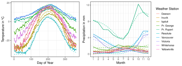
Figure 16: The ten observations of the bivariate Canadian weather data shown in Figure 6 (solid lines) and their reconstruction (dashed lines) based on the truncated Karhunen-Loève representation with estimates found by a weighted version of MFPCA (MFPCAweatherFit).

If elements are expanded in fixed basis functions, the number of basis functions that are needed to represent the data well will in general be quite high, particularly for elements with higher dimensional domains. As a consequence, the covariance matrix of all scores in step 2 of the estimation algorithm can become large and the eigendecompositions in step 3 can get computationally very demanding. By setting the option approx.eigen = TRUE, the eigenproblem is solved approximately using the augmented implicitly restarted Lanczos bidiagonalization algorithm (IRLBA, Baglama and Reichel, , 2005) implemented in the irlba package (Baglama et al., , 2018). The MFPCA function also implements nonparametric bootstrap on the level of functions to quantify the uncertainty in the estimation (cf. Happ and Greven, , 2018). Setting bootstrap = TRUE calculates pointwise bootstrap confidence bands for the principal component functions and bootstrap confidence bands for the associated eigenvalues.

5 Summary and outlook

The funData package implements functional data in an object-oriented manner. The aim of the package is to provide a flexible and unified toolbox for dense univariate and multivariate functional data with different dimensional domains as well as irregular functional data. The package implements basic utilities for creating, accessing and modifying the data, upon which other packages can be built. This distinguishes the funData package from other packages for functional data, that either do not provide a specific data structure together with basic utilities or mix this aspect with the implementation of advanced methods for functional data.

The funData package implements three classes for representing functional data based on the observed values and without any further assumptions such as basis function representations. The classes follow a unified approach for representing and working with the data, which means that the same methods are implemented for all the three classes (polymorphism). The package further includes a full simulation toolbox for univariate and multivariate functional data on one- and higher dimensional domains. This is a very useful feature when implementing and testing new methodological developments.

The MFPCA package is an example for an advanced methodological package, which builds upon the funData functionalities. It implements a new approach, multivariate functional principal component analysis for data on different dimensional domains (Happ and Greven, , 2018). All calculations relating to the functional data, data input and output use the basic funData classes and methods.

Both packages, funData and MFPCA, are publicly available on CRAN (https://CRAN.R-project.org) and GitHub (https://github.com/ClaraHapp). They come with a comprehensive documentation, including many examples. Both of them use the testthat system for unit testing (Wickham, , 2011), to make the software development more safe and stable and currently reach a code coverage of roughly $95\%$.

As potential future extensions, the funData package could also include irregFunData objects with observation points in a higher dimensional space or provide appropriate plotting methods for one-dimensional curves in 2D or 3D space. For the MFPCA, new basis functions as e.g., wavelets could be implemented.

Appendix

MFPCA: Additional Plots for the Case Study

Figure 17: Screeplots for visualizing the decrease of the eigenvalues for an MFPCAfit object, here obtained via screeplot(MFPCAweather). Left: The default plot (option type = "lines"). Right: The barplot version (type = "barplot").

Figure 18: The first principal component of the Canadian weather data as perturbation of the mean via plot(MFPCAweather, combined = TRUE). The plots show the effects of adding (’+’) and subtracting (’-’) a multiple of the principal component to the bivariate mean function.

Figure 19: The scores of the first two principal components of the Canadian weather data plotted via scoreplot(MFPCAweather). The labels give the names of the $35$ weather stations.

MFPCA: Univariate basis expansions

given: Given basis functions. This can for example be useful if a univariate FPCA was already calculated for each element. For one element, uniExpansions looks as follows:

R> list(type = "given", functions, scores, ortho)

Here functions is a funData object on the same domain as the data and contains the given basis functions. The parameters scores and ortho are optional. The first represents the coefficient matrix of the observed functions for the given basis functions in a row-wise manner, while ortho specifies whether the basis functions are orthonormal or not. If ortho is not supplied, the functions are treated as non-orthonormal.

uFPCA: Univariate functional principal component analysis for data on one-dimensional domains. This option was used in the previous example. The list entry for one element has the form:

R> list(type = "uFPCA", nbasis, pve, npc, makePD, cov.weight.type)

The implementation is based on the PACE approach (Yao et al., , 2005) with the mean function and the covariance surface smoothed with penalized splines (Di et al., , 2009), following the implementation in the refund package. The MFPCA function returns the smoothed mean function, while for all other options, the mean function is calculated pointwise. Options for this expansion include the number of basis functions nbasis used for the smoothed mean and covariance functions (defaults to 10; for the covariance this number of basis functions is used for each marginal); pve, a value between $0$ and $1$, giving the proportion of variance that should be explained by the principal components (defaults to $0.99$); npc, an alternative way to specify the number of principal components to be calculated explicitly (defaults to NULL, otherwise overrides pve); makePD, an option to enforce positive definiteness of the covariance surface estimate (defaults to FALSE) and cov.weight.type, which characterizes the weighting scheme for the covariance surface (defaults to "none").

spline1D and spline1Dpen: These options calculate a spline representation of functions on one-dimensional domains using the gam function in the mgcv package (Wood, , 2011, 2018). When using this option, the uniExpansions entry for one element is of the form:

R> list(type = "splines1D", bs, m, k)

R> list(type = "splines1Dpen", bs, m, k, parallel)

For spline1Dpen, the coefficients are found by a penalization approach, while for spline1D the observations are simply projected on the spline space without penalization. Thus, the spline1Dpen option will in general lead to smoother representations than spline1D. Possible options passed for these expansions are bs, the type of basis functions to use (defaults to "ps" for possibly penalized B-spline functions); m, the order of the spline basis (defaults to NA, i.e., the order is chosen automatically); k, the number of basis functions to use (default value is -1, which means that the number of basis functions is chosen automatically). For the penalized version, there is an additional option parallel which, if set to TRUE, calculates the spline coefficients in parallel. In this case, a parallel backend must be registered before (defaults to FALSE).

spline2D and spline2Dpen: These are analogue options to spline1D and spline1Dpen for functional data on two-dimensional domains (images):

R> list(type = "splines2D", bs, m, k)

R> list(type = "splines2Dpen", bs, m, k, parallel)

The parameters bs, m and k for the type, order and number of basis functions can be either a single number/character string that is used for all marginals or a vector with the specifications for all marginals. For the penalized version, the function bam in mgcv is used to speed up the calculations and reduce memory load. Setting parallel=TRUE enables parallel calculation of the basis function coefficients. As for the one-dimensional case, this requires a parallel backend to be registered before.

fda: This option allows to use all basis functions expansions implemented in the package fda, such as for example the leading $15$ basis functions of the Fourier basis on $[0,1]$:

R> basis <- fda::create.fourier.basis(c(0,1), nbasis=15)

R> list(type = "fda", basis)

All parameters are passed to the coercion method funData2fd, which heavily builds on the function eval.fd from the fda package. If this package is not available, an error is thrown and the calculation is stopped.

FCP_TPA: This option uses the Functional CP-TPA algorithm of Allen, (2013) to compute an eigendecomposition of image observations, which can be interpreted as functions on a two-dimensional domain. The algorithm assumes a CANDECOMP/PARAFRAC (CP) representation of the data tensor $X\in{\mathbb{R}}^{N\times S_{x}\times S_{y}}$ containing all observations $x_{i}$ with $S_{x}\times S_{y}$ pixels, each:

$$X=\sum_{m=1}^{M}d_{m}u_{m}\circ v_{m}\circ w_{m}$$

Here, $d_{m}$ is a scalar, $u_{m}\in{\mathbb{R}}^{N},v_{m}\in{\mathbb{R}}^{S_{x}},w_{m}\in{\mathbb{R}}^{S_{y}}$ are vectors and $\circ$ denotes the outer product. We can thus interpret $v_{m}\circ w_{m}$ as the $m$-th univariate eigenfunction evaluated at the same pixels as the originally observed data. The vector $d_{m}\cdot u_{m}\in{\mathbb{R}}^{N}$ can in turn be interpreted as the score vector containing the scores for the $m$-th principal component function and each observation. The algorithm proposed in Allen, (2013) includes smoothing parameters $\lambda_{u},\lambda_{v},\lambda_{w}\geq 0$ to smooth along all dimensions, extending the approach of Huang et al., (2009) from one-dimensional to two-dimensional functions. As smoothing along the observations $u_{m}\in{\mathbb{R}}^{N}$ is not required in the given context, the parameter $\lambda_{u}$ is fixed to zero and the smoothing is implemented only for the $v$ and $w$ directions. When decomposing images with this algorithm, the user has to supply a list of the following form for the corresponding element:

R> list(type = "FCP_TPA", npc, smoothingDegree, alphaRange,

+       orderValues, normalize)

Required options are npc, the number of eigenimages to be calculated, and alphaRange, the range of the smoothing parameters. The latter must be a list with two entries named v and w, giving the possible range for $\lambda_{v},\lambda_{w}$ as vectors with the minimal and maximal value, each (e.g., alphaRange = list(v = c(10^-2,10^2), w = c(10^-3,10^3)) would enforce $\lambda_{v}\in[10^{-2},10^{2}]$ and $\lambda_{w}\in[10^{-3},10^{3}]$). Optimal values for $\lambda_{v}$ and $\lambda_{w}$ are found by numerically optimizing a GCV criterion (cf. Huang et al., , 2009, in the one-dimensional case). Further options are the smoothing degree, i.e., the type of differences that should be penalized in the smoothing step (smoothingDegree, defaults to second differences for both directions) and two logical parameters concerning the ordering of the principal components and their normalizations: If orderValues is TRUE, the eigenvalues and associated eigenimages and scores are ordered decreasingly (defaults to TRUE), i.e., the first eigenimage corresponds to the highest eigenvalue that has been found, the second eigenimage to the second highest eigenvalue and so on. The option normalize specifies whether the eigenimages should be normalized (defaults to FALSE).

UMPCA: This option implements the UMPCA (Uncorrelated Multilinear Principal Component Analysis, Lu et al., , 2009) algorithm for finding uncorrelated eigenimages of two-dimensional functions (images). Essentially, this implements the UMPCA toolbox for MATLAB (Lu, , 2012) in R:

R> list(type = "UMPCA", npc)

The number of eigenimages that are calculated has to be supplied by the user (npc). Note that this algorithm aims more at uncorrelated features than at an optimal reconstruction of the images and thus may lead to unsatisfactory results for the MFPCA approach.

DCT2D/DCT3D: This option calculates a representation of functional data on two- or three-dimensional domains in a tensor cosine basis. For speeding up the calculations, the implementation is based on the fftw3 C-library (Frigo and Johnson, , 2005, developer version). If the fftw3-dev library is not available during the installation of the MFPCA package, the DCT2D and DCT3D options are disabled and throw an error. After installing fftw3-dev on the system, MFPCA has to be re-installed to activate DCT2D/DCT3D. The uniExpansions entry for a cosine representation of 2D/3D elements is:

R> list(type = "DCT2D", qThresh, parallel)

R> list(type = "DCT3D", qThresh, parallel)

The discrete cosine transformation is a real-valued variant of the fast Fourier transform (FFT) and usually results in a huge number of non-zero coefficients that mostly model “noise” and can thus be set to zero without affecting the representation of the data. The user has to supply a threshold between $0$ and $1$ (qThresh) that defines the proportion of coefficients to be thresholded. Setting e.g., qThresh = 0.9 will set $90\%$ of the coefficients to zero, leaving only the $10\%$ of the coefficients with the highest absolute values. The coefficients are stored in a sparseMatrix (package Matrix) object to reduce the memory load for the following computations. The calculations can be run in parallel for the different observations by setting the parameter parallel to TRUE (defaults to FALSE), if a parallel backend has been registered before.

References

- Allen, (2013) Allen, G. I. (2013). Multi-way functional principal components analysis. In IEEE 5th International Workshop on Computational Advances in Multi-Sensor Adaptive Processing (CAMSAP), pages 220–223.
- Armstrong, (2006) Armstrong, D. J. (2006). The quarks of object-oriented development. Commun. ACM, 49(2):123–128.
- Auguie, (2017) Auguie, B. (2017). gridExtra: Miscellaneous Functions for "Grid" Graphics. R package version 2.3.
- Baglama and Reichel, (2005) Baglama, J. and Reichel, L. (2005). Augmented implicitly restarted lanczos bidiagonalization methods. SIAM Journal on Scientific Computing, 27(1):19–42.
- Baglama et al., (2018) Baglama, J., Reichel, L., and Lewis, B. W. (2018). irlba: Fast Truncated SVD, PCA and Symmetric Eigendecomposition for Large Dense and Sparse Matrices. R package version 2.3.2.
- Bates and Maechler, (2018) Bates, D. and Maechler, M. (2018). Matrix: Sparse and Dense Matrix Classes and Methods. R package version 1.2-14.
- Booch et al., (2007) Booch, G., Maksimchuk, R. A., Engle, M. W., Young, B. J., Conallen, J., and Houston, K. A. (2007). Object-Oriented Analysis and Design with Applications. Addison-Wesley, Upper Saddle River, NJ, 3rd edition.
- Bouveyron, (2015) Bouveyron, C. (2015). funFEM: Clustering in the Discriminative Functional Subspace. R package version 1.1.
- Brockhaus and Ruegamer, (2018) Brockhaus, S. and Ruegamer, D. (2018). FDboost: Boosting Functional Regression Models. R package version 0.3-2.
- Cederbaum, (2018) Cederbaum, J. (2018). sparseFLMM: Functional Linear Mixed Models for Irregularly or Sparsely Sampled Data. R package version 0.2.2.
- Chambers, (2008) Chambers, J. M. (2008). Software for Data Analysis. Springer-Verlag, New York.
- Dai et al., (2018) Dai, X., Hadjipantelis, P. Z., Han, K., and Ji, H. (2018). fdapace: Functional Data Analysis and Empirical Dynamics. R package version 0.4.0.
- Di et al., (2009) Di, C.-Z., Crainiceanu, C. M., Caffo, B. S., and Punjabi, N. M. (2009). Multilevel Functional Principal Component Analysis. The Annals of Applied Statistics, 3(1):458–488.
- Febrero-Bande and Oviedo de la Fuente, (2012) Febrero-Bande, M. and Oviedo de la Fuente, M. (2012). Statistical computing in functional data analysis: The R package fda.usc. Journal of Statistical Software, 51(4):1–28.
- Frigo and Johnson, (2005) Frigo, M. and Johnson, S. G. (2005). The design and implementation of FFTW3. Proceedings of the IEEE, 93(2):216–231.
- Goldsmith et al., (2013) Goldsmith, J., Greven, S., and Crainiceanu, C. (2013). Corrected Confidence Bands for Functional Data Using Principal Components. Biometrics, 69(1):41–51.
- Goldsmith et al., (2018) Goldsmith, J., Scheipl, F., Huang, L., Wrobel, J., Gellar, J., Harezlak, J., McLean, M. W., Swihart, B., Xiao, L., Crainiceanu, C., and Reiss, P. T. (2018). refund: Regression with Functional Data. R package version 0.1-17.
- Gregorutti, (2016) Gregorutti, B. (2016). RFgroove: Importance Measure and Selection for Groups of Variables with Random Forests. R package version 1.1.
- (19) Happ, C. (2018a). funData: An S4 Class for Functional Data. R package version 1.3.
- (20) Happ, C. (2018b). MFPCA: Multivariate Functional Principal Component Analysis for Data Observed on Different Dimensional Domains. R package version 1.3.
- Happ and Greven, (2018) Happ, C. and Greven, S. (2018). Multivariate functional principal component analysis for data observed on different (dimensional) domains. Journal of the American Statistical Association, 113:649–659.
- Huang et al., (2009) Huang, J. Z., Shen, H., and Buja, A. (2009). The Analysis of Two-Way Functional Data Using Two-Way Regularized Singular Value Decompositions. Journal of the American Statistical Association, 104(488):1609–1620.
- Huo et al., (2014) Huo, L., Reiss, P., and Zhao, Y. (2014). refund.wave: Wavelet-Domain Regression with Functional Data. R package version 0.1.
- Lila et al., (2016) Lila, E., Sangalli, L. M., Ramsay, J., and Formaggia, L. (2016). fdaPDE: Functional Data Analysis and Partial Differential Equations; Statistical Analysis of Functional and Spatial Data, Based on Regression with Partial Differential Regularizations. R package version 0.1-4.
- Lu, (2012) Lu, H. (2012). Uncorrelated Multilinear Principal Component Analysis (UMPCA). MATLAB Central File Exchange. Version 1.0.
- Lu et al., (2009) Lu, H., Plataniotis, K. N., and Venetsanopoulos, A. N. (2009). Uncorrelated multilinear principal component analysis for unsupervised multilinear subspace learning. IEEE Transactions on Neural Networks, 20(11):1820–1836.
- Meyer, (1988) Meyer, B. (1988). Object Oriented Software Construction. Prentice Hall, New York.
- Peng and Paul, (2011) Peng, J. and Paul, D. (2011). fpca: Restricted MLE for Functional Principal Components Analysis. R package version 0.2-1.
- Ramsay and Silverman, (2005) Ramsay, J. O. and Silverman, B. W. (2005). Functional Data Analysis. Springer-Verlag, New York, 2nd edition.
- Ramsay et al., (2018) Ramsay, J. O., Wickham, H., Graves, S., and Hooker, G. (2018). fda: Functional Data Analysis. R package version 2.4.8.
- Scheipl and Greven, (2016) Scheipl, F. and Greven, S. (2016). Identifiability in Penalized Function-on-Function Regression Models. Electronic Journal of Statistics, 10(1):495–526.
- Schmutz et al., (2018) Schmutz, A., Jacques, J., and Bouveyron, C. (2018). funHDDC: Univariate and Multivariate Model-Based Clustering in Group-Specific Functional Subspaces. R package version 2.1.0.
- Shang and Hyndman, (2016) Shang, H. L. and Hyndman, R. J. (2016). rainbow: Rainbow Plots, Bagplots and Boxplots for Functional Data. R package version 3.4.
- Soueidatt, (2014) Soueidatt, M. (2014). Funclustering: A Package for Functional Data Clustering. R package version 1.0.1.
- Tarabelloni et al., (2018) Tarabelloni, N., Arribas-Gil, A., Ieva, F., Paganoni, A. M., and Romo, J. (2018). roahd: Robust Analysis of High Dimensional Data. R package version 1.4.
- Tucker, (2017) Tucker, J. D. (2017). fdasrvf: Elastic Functional Data Analysis. R package version 1.8.3.
- Wang and Marron, (2007) Wang, H. and Marron, J. S. (2007). Object Oriented Data Analysis: Sets of Trees. The Annals of Statistics, 35(5):1849–1873.
- Wang et al., (2016) Wang, J.-L., Chiou, J.-M., and Müller, H.-G. (2016). Functional data analysis. Annual Review of Statistics and Its Application, 3(1):257–295.
- Wickham, (2009) Wickham, H. (2009). ggplot2: Elegant Graphics for Data Analysis. Springer-Verlag, New York.
- Wickham, (2011) Wickham, H. (2011). testthat: Get started with testing. The R Journal, 3(1):5–10.
- Wickham et al., (2018) Wickham, H., Chang, W., Henry, L., Pedersen, T. L., Takahashi, K., Wilke, C., Woo, K., and RStudio (2018). ggplot2: Create Elegant Data Visualisations Using the Grammar of Graphics. R package version 3.0.0.
- Wood, (2011) Wood, S. N. (2011). Fast Stable Restricted Maximum Likelihood and Marginal Likelihood Estimation of Semiparametric Generalized Linear Models. Journal of the Royal Statistical Society B, 73(1):3–36.
- Wood, (2018) Wood, S. N. (2018). mgcv: Mixed GAM Computation Vehicle with GCV/AIC/REML Smoothness Estimation. R package version 1.8-24.
- Yao et al., (2005) Yao, F., Müller, H.-G., and Wang, J.-L. (2005). Functional Data Analysis for Sparse Longitudinal Data. Journal of the American Statistical Association, 100(470):577–590.
- Yassouridis, (2018) Yassouridis, C. (2018). funcy: Functional Clustering Algorithms. R package version 1.0.0.
- Zeileis and Grothendieck, (2005) Zeileis, A. and Grothendieck, G. (2005). zoo: S3 infrastructure for regular and irregular time series. Journal of Statistical Software, 14(6):1–27.
- Zeileis et al., (2018) Zeileis, A., Grothendieck, G., Ryan, J. A., Ulrich, J. M., and Andrews, F. (2018). zoo: S3 Infrastructure for Regular and Irregular Time Series (Z’s Ordered Observations). R package version 1.8-3.