Particle Dynamics Around the Black String

Abstract

In this paper, some dynamical properties of neutral and charged particles around a weakly magnetized five-dimensional static black string have been studied. The perturbation method was also used to calculate the Innermost Stable Circular Orbit (ISCO) of this metric in the presence of a magnetic field. The escape velocity of neutral and charged particles around the black string was derived. In the next step, the analytical solutions of the equations of motion were discussed and some possible orbits for particles in the black string space-time were plotted. Interestingly, it was found that adding an extra dimension has a slight influence on the effective potential and one term of the effective force. The magnitude of the new constant of motion $(J)$ affects both the shape of the potential and existence of the stable circular orbits. In conclusion, by comparing a black hole and a black string, it is realized that the value of a new constant of motion causes slight but interesting differences.

I INTRODUCTION

Within the last few decades, higher-dimensional space-times have received special attention in theoretical physics ArkaniHamed:1998rs -Kaya:2007kh . Notable attempts to unify fundamental forces, such as Kaluza and Klein theory, and some other interesting theories of physics such as String theory or Brane cosmology, were necessarily formulated in such higher-dimensional space-times Lee:2006jx -Obers:2008pj . To investigate the properties of extra dimensions, studying the higher-dimensional solutions of Einstein equations (like black strings) is considered Lee:2006jx , Kunz:2014zxa , Kleihaus:2006ee . While there are different methods to find the exact solution of Einstein gravity in five-dimensional space-time, the common methods in more than five-dimensional space-times, are numerical or perturbational Kleihaus:2016kxj . There are also several studies about the various features of the higher-dimensional space-times, such as the equation of motion in 5-dimensional space-time Mashhoon:1994iu -Seahra:2003eb , the possibility of detecting extra dimension and its relation to Einstein’s Equivalence Principle Wesson:1997dq -Wesson:2013nk , the physical properties of 5-dimensional space-time Wesson:1994pj , the properties of higher-dimensional black holes (charged and rotating ones) Kleihaus:2007kc , Kunz:2006zz , the solar system test of 5-dimensional gravity Kalligas:1994vf , Liu:2000zq , and even some suggested experimental way to explore extra dimension by spectroscopy Luo:2006ad .

Tangherlini investigated the higher-dimensional black hole for the first time in 1963 Tangherlini:1963 . This idea was followed by Myers-Perry Myers:1986 for the rotating black hole, and the simple form of 5-dimensional black string was investigated by Gregory and Laflamme in 1987 Gregory:1987nb , which has been obtained by adding one non-compact extra dimension to Schwarzschild black hole and called Black String Lee:2006jx . By considering the non-compact extra dimension the topology of the horizon will be $R^{1}\times S^{2}$. There is also another option, adding a compact flat extra dimension to a Schwarzschild black hole that changes the horizon topology to $S^{1}\times S^{2}$ and is called a black ring Kunz:2014zxa , Kleihaus:2016kxj . With a compact extra dimension, there is a classification of the spherically symmetric string-like vacuum solution in 5-dimensional space-time Chodos:1980df . One interesting form of this classification is a stationary string-like solution of the Einstein equation in (4+1) dimensions, which has been investigated Kim:2007ek and has shown some interesting features that may help solve the stability problem(Marolf:2005vn , Horowitz:2001cz ) of the black string solution. Also, the motion of massive test particles in static spherically symmetric magnetic-free 5-dimensional space-time has been investigated Lacquaniti:2009wc . Other theories like Space-Time-Matter (STM) theory Wesson:1999 -Liu:2007wx consider a non-compact fifth dimension. Some interesting investigations conducted on the astrophysical implication in the STM framework Liu:2000zq , Liu:2007wx , Liu:1996hs , Liu:1992bp . There is also another kind of cosmological model in 5 dimensions called brane world (Membrane theory) Brax:2003fv , Langlois:2002bb .

Lately, great interests were shown in exploring some aspects of the black strings in the context of different modified gravity models. For example, there are several studies on the effect of the perturbation on black strings in the de Rham-Gabadadze-Tolley (dRGT) gravity Ponglertsakul:2018smo , the role of the cosmological constant in thermodynamic properties of black string Gim:2018aix , and the validity of entropy formula in Einstein-Maxwell-Dilaton (EMD) theory for the black string Setare:2018yfu . Also, there is a tendency to extend and apply the Anti-de Sitter/Conformal theory to different areas of physics and since the black objects like black strings in asymptotically Anti-de Sitter (AdS) space are noted subjects in holographic duality viewpoint, there are several studies on this topic Ponglertsakul:2018smo -Nakas:2019rod . Other current works on black string are: The study of black string properties in different higher dimensional theories like Lovelock theories Giacomini:2018sho , and the investigation of black strings in modified gravities like Chern-Simons modified gravity (CSMG) Cisterna:2018jsx .

Studying how the massive and massless particles move around the black objects is a common method to probe the gravitational fields around them Hackmann:2009rp . In four-dimensional space-time, there are lots of studies that widely analyze particle motions, such as what has investigated how the charged and neutral particles move near the weakly magnetized Schwarzschild black hole and their bounded trajectories Frolov:2010mi , and the dynamics of a charged particle in the magnetized Janis-Newman-Winicour space-time Babar:2015kaa . Besides, the particle’s motion around a (2+1)-dimensional BTZ (Banados, Teitelboim, Zanelli) black hole Soroushfar:2015dfz and geodesic equations in dilaton black holes Soroushfar:2016yea have studied. Other extended forms of a Schwarzschild black hole, such as the Reissner-Nordstrom black hole has also studied in magnetized and non-magnetized space-times Majeed:2014kka . It has been shown that the cosmic string might be detected by analyzing the orbits of a test particle around of a Kerr black hole pierced by a cosmic string Hackmann:2010ir , such as how the charged particles move around the five-dimensional rotating black hole, how a magnetic field affects this space-time explored Kaya:2007kh , Grunau:2013oca , how the energy of collision of two massive particles impact in the static, rotating and magnetized black string Tursunov:2013zha , and the solution of geodesic equations of a Schwarzschild black hole pierced by a cosmic string for both massive and massless particles Hackmann:2009rp .

Both theoretical and experimental studies show that the existence of magnetic fields around the black holes ( due to the presence of accretion disk’s plasma Frolov:2010mi ,Akiyama:2019fyp ) would leave an impact on particle motions around the black objects. However, in most cases while the magnetic field around the event horizon of a black hole is not strong enough to disturb the geometry of the black hole, it would affect the motion of charged particles around it. Therefore, the magnetic features of black holes are taken into consideration in studies Frolov:2010mi ,Majeed:2014kka ,Wald:1974np . Also, it has been shown that the magnetic field has an important impact on the existence of stable circular orbits in five-dimensional space-time. Although there exist stable circular orbits around the four-dimensional rotating black holes for massive particles, there are no such orbits in five-dimensional one in the absence of a magnetic field. However, in the presence of a magnetic field, there could be such orbits for both rotating and non-rotating black holes in five dimensions Kaya:2007kh .

All of these points motivated us to study the massive particle dynamics around a static black string. In this article, we first found the effective potential of a static black string, with a non-compact extra dimension, and the equations of motion for time-like particles in the absence of a magnetic field. Then by adding a magnetic field, new dynamical equations for charged particles were found. Also, the ISCO in the dimensionless form of dynamical equations for a massive test particle was calculated. Then, we studied how the shape of effective potential could be influenced by the constants of motion, especially by the new constant of motion, we also investigated the manner in which they influence the existence of ISCO for a massive test particle in this metric. We calculated the escape velocity of the neutral and charged particles in certain conditions and analyzed the effects of different constants of motions in relation to the escape velocity and the distance of the particle from the black string. Finally, the analytical solutions of the equations of motion were discussed, and some possible orbits for particles in the black string space-time were plotted.

II Particles Around Black String

In this section, we study how a massive particle moves around a static black string space-time. This metric obtains by adding an extra infinite spatial dimension $\omega$ to the Schwarzschild space-time and the resulting space-time is axially symmetric.

II.1 Metric In the Absence of Magnetic Field

Before finding the equations of motion of a massive test particle moving in the vicinity of a weakly magnetized black string, let us present results for a simpler case of a magnetic field-free condition. According to Gregory and Laflamme model, the five-dimensional metric is Gregory:1987nb :

$$ds^{2}=-F(r)dt^{2}+\frac{dr^{2}}{F(r)}+r^{2}(d\theta^{2}+sin^{2}\theta d\varphi^{2})+d\omega^{2},$$ (1)

where

$$F(r)=1-\dfrac{2M}{r},$$ (2)

in which $\omega$ represents the new dimension, and $M$ is the mass of the black string and the gravitational constant and the light velocity are adjusted to 1, $G=c=1$ Lee:2006jx , Grunau:2013oca . There is more than one independent angular momentum in higher-dimensional axially symmetric space-times Kunz:2014zxa . In the case of five-dimensional space-time, there are two independent angular momentums $L_{z}$ and $J$ related to the test particle. These momentums are associated with the rotation of orthogonal independent spatial planes around the two axes. For instance, $\theta=\frac{\pi}{2}$ plane is orthogonal to both z-axis (in Cartesian coordinate) and the fifth dimension axis. Besides, Killing vectors are obtained as Lacquaniti:2009wc , Frolov:2010mi , Majeed:2014kka , Zahrani:2013up :

$$\xi_{(t)}^{\mu}\partial_{\mu}=\partial_{t},~{}~{}\xi_{(t)}^{\mu}=(1,0,0,0,0),$$

$$\xi_{(\varphi)}^{\mu}\partial_{\mu}=\partial_{\varphi},~{}~{}\xi_{(\varphi)}^{\mu}=(0,0,0,1,0),$$

$$\xi_{(\omega)}^{\mu}\partial_{\mu}=\partial_{\omega},~{}~{}\xi_{(\omega)}^{\mu}=(0,0,0,0,1).$$ (3)

Therefore, there are three conserved quantities associated with the Killing vectors, the energy( per unit mass) $\varepsilon$ of the moving particle, the component of the angular momentum of the particle that is aligned with z-axis $L_{z}$ and the angular momentum $J$, which is the new constant of motion according to the extra dimension $\omega$.

$$\varepsilon \equiv -\dfrac{P_{\mu}\xi_{(t)}^{\mu}}{m}=\dot{t}~{}F(r),$$

$$L_{z} \equiv \dfrac{P_{\mu}\xi_{(\varphi)}^{\mu}}{m}=\dot{\varphi}~{}r^{2}~{}{\sin^{2}\theta},$$

$$J \equiv \dfrac{P_{\mu}\xi_{(\omega)}^{\mu}}{m}=\dot{\omega},$$ (4)

where $P^{\mu}=mu^{\mu}$ is the five-momentum in which $u^{\mu}$ is the five-velocity, $m$ is the mass of the particle, and the over dot denotes the derivative with respect to the proper time ($\tau$).

Using the invariance condition ${g_{\mu\nu}\dot{x}^{\mu}\dot{x}^{\nu}\equiv\epsilon}$, the constraint equation obtains as:

$$\dfrac{ds^{2}}{d\tau^{2}}=\epsilon\Longrightarrow\epsilon F(r)=\dot{r}^{2}-\dot{t}^{2}~{}F(r)^{2}+r^{2}F(r)\dot{\theta}^{2}+r^{2}F(r){\sin^{2}\theta}\dot{\varphi}^{2}+F(r)\dot{\omega}^{2}.$$ (5)

According to Eq. (II.1) :

$$\dot{r}^{2}=\varepsilon^{2}-r^{2}F(r)\dot{\theta}^{2}-F(r)(-\epsilon+J^{2}+\frac{{L_{z}}^{2}}{r^{2}{\sin^{2}\theta}}).$$ (6)

and by defining effective potential as:

$$U_{eff}=F(r)(-\epsilon+J^{2}+\frac{{L_{z}}^{2}}{r^{2}{\sin^{2}\theta}}),$$ (7)

obtains:

$$\dot{r}^{2}=\varepsilon^{2}-r^{2}F(r)\dot{\theta}^{2}-U_{eff}.$$ (8)

where ${\epsilon=-1,0}$ are for time-like and null geodesics respectively. Eq. (7)shows that the $F(r)J^{2}$ term is the only difference between the effective potential in four and five-dimensional space-times Zahrani:2013up .

The geodesic equation (for a neutral particle) is:

$$\ddot{x}^{\mu}+\Gamma_{\nu\sigma}^{\mu}\dot{x}^{\nu}\dot{x}^{\sigma}=0.$$ (9)

Then, the equations of motion of time-like particles are:

$$\ddot{r}=(r-3M)\dot{\theta}^{2}+(r-3M)\frac{{L_{z}}^{2}}{r^{4}{\sin^{2}\theta}}-\frac{M}{r^{2}}(1+J^{2}),$$ (10)

$$\ddot{\theta}=-\frac{2}{r}\dot{r}\dot{\theta}+\frac{{L_{z}}^{2}\cos{\theta}}{r^{4}{\sin^{3}\theta}}.$$ (11)

There is no explicit relation between $J$ and $\ddot{\theta}$, though $J$ implies its effect through $\dot{r}$ and $\dot{\theta}$.

II.2 Presence of Magnetic Field

Here, we study the effect of an external magnetic field on the motion of test particles with electric charge $q$ around a black string. Also, possible magnetic fields along each of the z-axis or $\omega$-axis may be considered to track the test particle trajectory. Our premise is a static, axisymmetric and homogeneous magnetic field at the spatial infinity in the vicinity of black string, which is directed along the z-axis. In the presence of magnetic field the Lagrangian of the moving particle is:

$$\mathfrak{L}=\dfrac{1}{2}g_{\mu\nu}\dot{x}^{\mu}\dot{x}^{\nu}+\dfrac{q}{m}A_{\mu}\dot{x}^{\mu},$$ (12)

where ${m}$ and ${q}$ are mass and charge of particle respectively. The 5-potential ${A^{\mu}}$ for this metric is constructed from the Killing vectors of the black string space-time. The Killing vectors obey ${\square\xi^{\mu}=0}$, similar to the Maxwell equation for 4-potential in the Lorenz gauge ${A^{\mu}_{;\mu}=0}$ Frolov:2010mi , Majeed:2014kka , Wald:1974np , Aliev:2002nw :

$$A^{\mu}=\dfrac{\mathfrak{B}}{2}\xi^{\mu}_{(\varphi)}-\dfrac{Q}{2m}\xi^{\mu}_{(t)}+\alpha\xi^{\mu}_{(\omega)},$$ (13)

in which Q is the charge of black string that in our case is zero and $\alpha$ is an arbitrary constant and since there is not any coupling among $\omega$ and other coordinates, it could be considered as zero too Aliev:2002nw , and ${\mathfrak{B}}$ is the magnetic field strength and the 2-form magnetic field, with respect to an observer whose 5-velocity is $u_{\nu}$ McDavid:2006sq :

$$\mathfrak{B}^{\mu\eta}=-\dfrac{1}{2}~{}e^{\mu\eta\nu\lambda\sigma}~{}F_{\lambda\sigma}~{}u_{\nu},$$ (14)

where ${e^{\mu\eta\nu\lambda\sigma}=\dfrac{\epsilon^{\mu\eta\nu\lambda\sigma}}{\sqrt{-g}},~{}\epsilon_{01234}=1,~{}g=det(g_{\mu\nu})}$. The Maxwell tensor ${F_{\mu\nu}}$ is defined as McDavid:2006sq :

$$F_{\mu\nu}=A_{\nu,\mu}-A_{\mu,\nu}=A_{\nu;\mu}-A_{\mu;\nu}.$$ (15)

By considering Eq. (II.1) and Eq. (13) one can see that the 5-potential ${A^{\mu}}$ is invariant with respect to the Killing vector isometries McDavid:2006sq :

$$(L_{\xi}A)_{\mu}=A_{\mu,\nu}\xi^{\nu}+A_{\nu}\xi^{\nu}_{,\mu}=0.$$ (16)

The conserved quantities associated with these symmetries are obtained as Frolov:2010mi , Majeed:2014kka :

$$\varepsilon \equiv -\dfrac{P_{\mu}\xi_{(t)}^{\mu}}{m}=\dot{t}~{}F(r),$$

$$L_{z} \equiv \dfrac{P_{\mu}\xi_{(\varphi)}^{\mu}}{m}=(\dot{\varphi}+B)~{}r^{2}~{}{\sin^{2}\theta},$$

$$J \equiv \dfrac{P_{\mu}\xi_{(\omega)}^{\mu}}{m}=\dot{\omega},$$ (17)

where ${P^{\mu}=mu^{\mu}+qA^{\mu}}$ ,and $q$ is the charge of the particle and:

$$B=\dfrac{q\mathfrak{B}}{2m}.$$ (18)

By using the normalization condition, and similar to Eq. (5), we obtain the effective potential for the charged time-like particle in the presence of a magnetic field as:

$$\dot{r}^{2}=\varepsilon^{2}-r^{2}F\dot{\theta}^{2}-F(r)[-\epsilon+J^{2}+r^{2}\sin^{2}\theta(\dfrac{L_{z}}{r^{2}\sin^{2}\theta}-B)^{2}],$$ (19)

$$U_{eff}=F(r)[-\epsilon+J^{2}+r^{2}\sin^{2}\theta(\dfrac{L_{z}}{r^{2}\sin^{2}\theta}-B)^{2}].$$ (20)

As we know, the equation of motion of the charged particle in an electromagnetic field ${F_{\mu\nu}}$ is Frolov:2010mi , Majeed:2014kka :

$$\ddot{x}^{\mu}+\Gamma_{\nu\sigma}^{\mu}\dot{x}^{\nu}\dot{x}^{\sigma}=\dfrac{q}{m}F_{\alpha}^{\mu}\dot{x}^{\alpha}.$$ (21)

Therefore, the dynamical equations in black string metric are:

$$\ddot{r}=(r-3M)\dot{\theta}^{2}+(r-3M)\dfrac{L_{z}^{2}}{r^{4}\sin^{2}\theta}+\dfrac{2M}{r^{2}}BL_{z}-(r-M)\sin^{2}\theta B^{2}-\dfrac{M}{r^{2}}(1+J^{2}),$$ (22)

$$\ddot{\theta}=-\dfrac{2}{r}\dot{r}\dot{\theta}+\dfrac{L_{z}^{2}\cos\theta}{r^{4}\sin^{3}\theta}-B^{2}\sin{\theta}\cos{\theta}.$$ (23)

Similar to the magnetic field free case, the $\ddot{\theta}$ is independent of the new angular momentum $J$.

III Dimensionless Dynamical Equations

For more simplification, one can rewrite the dynamical equations in dimensionless form, by using these definitions Frolov:2010mi , Majeed:2014kka , Zahrani:2013up :

$$\sigma=\dfrac{\tau}{2M},~{}~{}\rho=\dfrac{r}{2M},~{}~{}l_{z}=\dfrac{L_{z}}{2M},~{}~{}\Omega=\dfrac{\omega}{2M},~{}~{}b=2BM,~{}~{}\acute{m}=\dfrac{m}{2M}.$$ (24)

So the Eq. (22) and Eq. (23) are expressed as follows:

$$\dfrac{d^{2}\theta}{d\sigma^{2}}=-\dfrac{2}{\rho}\dfrac{d\rho}{d\sigma}\dfrac{d\theta}{d\sigma}+\dfrac{l_{z}^{2}\cos\theta}{\rho^{4}\sin^{3}\theta}-b^{2}\sin\theta\cos\theta,$$ (25)

$$\dfrac{d^{2}\rho}{d\sigma^{2}}=\dfrac{1}{2}(2\rho-3)({\dfrac{d\theta}{d\sigma}})^{2}+\dfrac{2bl_{z}-1}{2\rho^{2}}+\dfrac{l_{z}^{2}(2\rho-3)}{2\rho^{4}\sin^{2}\theta}-\dfrac{b^{2}}{2}(2\rho-1)\sin^{2}\theta-\dfrac{J^{2}}{2\rho^{2}},$$ (26)

and the Eq. (19) for time-like geodesics (${\epsilon=-1}$) changes to:

$${(\dfrac{d\rho}{d\sigma})}^{2}=\varepsilon^{2}-\rho^{2}(1-\dfrac{1}{\rho}){(\dfrac{d\theta}{d\sigma})}^{2}-U_{eff},$$ (27)

in which:

$$U_{eff}=(1-\dfrac{1}{\rho})[1+J^{2}+\dfrac{({l_{z}-b\rho^{2}\sin^{2}\theta})^{2}}{\rho^{2}\sin^{2}\theta}].$$ (28)

Extending some four-dimensional cases in the planetary motion of test particle studies Frolov:2010mi , Majeed:2014kka , Zahrani:2013up to five-dimensional analysis, we choose $\theta=\dfrac{\pi}{2}$ plane as our test particle’s trajectory plane.

III.1 The Innermost Stable Circular Orbit

According to Eq. (28) and as it is shown in the next section the angular momentum has the role of a defining parameter of the shape of potential Jefremov:2015gza . Besides, like its important role in the shape of potential in the Schwarzschild black hole Jefremov:2015gza , Frolov:2010mi , the amount of ${l_{z}}$ determines if the 5-dimensional effective potential has both a minimum and a maximum, only one extremum, or no extremums at all. So, to find the innermost stable circular orbits (ISCO), we not only need to find ${\rho_{ISCO}}$, but also ${l_{zISCO}}$. In fact, we consider the series of mentioned conditions of circular motion in ref. Jefremov:2015gza , to find ISCO parameters:

(i) Firstly, in circular motion the radial velocity must be zero so: ${\dfrac{d\rho}{d\tau}=0}$.

(ii) Secondly, the acceleration along the radial coordinate should be zero: ${\dfrac{d^{2}\rho}{d\tau^{2}}=0}$.

(iii) Thirdly, the second derivative of effective potential must be zero in an inflection point.

All of these conditions must be satisfied, simultaneously. Our equations of energy and effective potential in the presence of magnetic field are Eq. (27) and Eq. (28). The first condition (in the ${\theta=\dfrac{\pi}{2}}$ plane) leads to ${\varepsilon^{2}=U_{eff}}$ and the second one leads to:

$$U_{,\rho}=l_{z}^{2}(3-2\rho)-2bl_{z}\rho^{2}+\rho^{2}[1+J^{2}+b^{2}\rho^{2}(2\rho-1)]=0,$$ (29)

where ${"_{,\rho}"=\dfrac{\partial}{\partial\rho}}$ , and the third one is:

$$U_{,\rho\rho}=2\left[\rho^{2}(b^{2}\rho^{3}-J^{2}-1)+2bl_{z}\rho^{2}+3l_{z}^{2}(\rho-2)\right]=0.$$ (30)

where ${"_{,\rho\rho}"=\dfrac{\partial^{2}}{\partial\rho^{2}}}$. In general, finding the exact inflection point of Eq. (29) is hard and it should be solved numerically Jefremov:2015gza . Therefore, we choose the perturbation method that has been suggested in Jefremov:2015gza . We presume that although the magnetic field near the black string can disturb it, yet its magnitude is small enough ${(b\ll 1)}$ to use the perturbation method. ISCO parameters in the absence of magnetic field are ${\rho_{0}}$, ${l_{z0}}$ and ${\varepsilon_{0}}$:

$$\rho_{0}=3,$$ (31)

$$l_{z0}=\pm\sqrt{3(1+J^{2})},$$ (32)

$$\varepsilon_{0}=\dfrac{2\sqrt{2}}{3}\sqrt{1+J^{2}}.$$ (33)

This shows that, among these three parameters, only ${l_{z0}}$ and ${\varepsilon_{0}}$ are related to the $J$. By choosing:

$$\rho=\rho_{0}+b\rho_{1}+b^{2}\rho_{2},$$ (34)

$$l_{z}=l_{z0}+bl_{z1}+b^{2}l_{z2},$$ (35)

$$\varepsilon=\varepsilon_{0}+b\varepsilon_{1}+b^{2}\varepsilon_{2},$$ (36)

and substituting them in ${U_{,\rho}=0}$, ${U_{,\rho\rho}=0}$ and neglecting the third order of the perturbation, the results are:

$$\rho_{1}=0,~{}~{}l_{z1}=-3,~{}~{}\varepsilon_{1}=\mp\dfrac{\sqrt{3}}{3},$$ (37)

$$\rho_{2}=\dfrac{-216}{1+J^{2}},~{}~{}l_{z2}=\dfrac{\mp 72}{\sqrt{3(1+J^{2})}},~{}~{}\varepsilon_{2}=\dfrac{8}{\sqrt{2(1+J^{2})}},$$ (38)

so:

$$\rho=3-\dfrac{216}{1+J^{2}}b^{2},$$ (39)

$$l_{z}=\pm\sqrt{3(1+J^{2})}-3b\mp\dfrac{72}{\sqrt{3(1+J^{2})}}b^{2},$$ (40)

$$\varepsilon=\dfrac{2\sqrt{2}}{3}\sqrt{1+J^{2}}\mp\dfrac{\sqrt{3}}{3}b+\dfrac{8}{\sqrt{2(1+J^{2})}}b^{2}.$$ (41)

Up to the first order of perturbation, these equations show that the radius of ISCO in Schwarzschild black hole is similar to that of the black string, and the fifth dimension has its effect on ${l_{z}}$ and ${\varepsilon}$ via new angular momentum $J$. Here we have three parameters $l_{z}$, $J$, $\varepsilon$ which are constants of motion. We assume ${J}$ as our degree of freedom parameter and tuned it in a way that helps us find the other two parameters. Now, in general condition and similar to Frolov:2010mi , by adding Eq. (29) and Eq. (30) we can eliminate ${J}$ and find ${l_{z}}$ in terms of ${b}$:

$$l_{z\pm}=\pm b\rho^{2}\left[\dfrac{1-3\rho}{\rho-3}\right]^{\dfrac{1}{2}},$$ (42)

in which, ${l_{z-}}$ shows that the Lorentz force is attractive and ${l_{z+}}$ how the Lorentz force is repulsive Frolov:2010mi , Babar:2015kaa , Zahrani:2013up . Now by substituting Eq. (42) into Eq. (30) we can find parameter ${b}$ in terms of ${\rho}$ and ${J}$:

$$b=\dfrac{\sqrt{2(3-\rho)(1+J^{2})}}{2\rho\left[4\rho^{2}-9\rho+3\pm\sqrt{(3-\rho)(3\rho-1)}\right]^{\dfrac{1}{2}}}.$$ (43)

It shows that the new constant of motion, related to the fifth dimension, is not separable from both ${b}$ and ${l_{z}}$. Comparing Eq.(42) and Eq.(40) one can see that adding a fifth dimension shows its effects on ${l_{z}}$ directly Eq.(40) or via ${b}$ in Eq.(42). Now by putting Eq.(43) in Eq.(42), ${l_{z}}$ in terms of ${\rho}$ will be obtained:

$$l_{z}=\pm\dfrac{\rho\sqrt{(3\rho-1)(1+J^{2})}}{\sqrt{2}\left[4\rho^{2}-9\rho+3\pm\sqrt{(3-\rho)(3\rho-1)}\right]^{\dfrac{1}{2}}}.$$ (44)

Eq.(43) and Eq.(44) show the combinations among parameters $b$, $l_{z}$ and $J$. Also, in the case of $J=0$, these results are in accordance with the four-dimensional black hole results which were already obtained in Frolov:2010mi , Zahrani:2013up .

Since we have only two constraint equations ($U_{,\rho\rho}=0$, $U_{,\rho}=0$), we cannot express their relations to $\rho$ separately. So, we have to fix one of them ($b$, $l_{z}$, $J$). According to our decision for choosing a small magnetic field, we chose ${b=0.5}$ (fixed).

IV Effective Potential

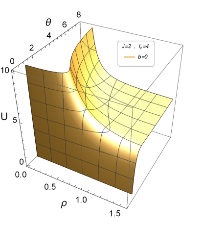
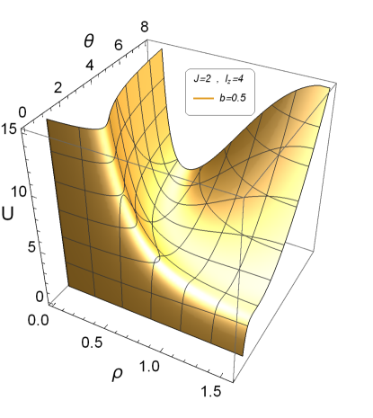
Figure 1: Effective Potential versus $\rho$ and ${\theta}$ in $J=2$ and $l_{z}=4$ for (a) $b=0$, (b) $b=0.5$.

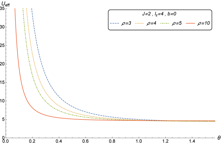
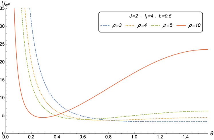
Figure 2: Effective Potential versus ${\theta}$

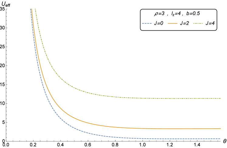
Figure 3: Effective Potential versus ${\theta}$ in $\rho=3$, $b=0.5$ and $l_{z}=4$ for $J=0$ (blue dashed), $J=2$ (orange line), $J=4$ (green dot dashed).

To study the effective potential of the black string and its properties, we consider that the strength of the magnetic field and the mass of the black string are fixed. Thus, based on Eq.(28), the effective potential depends on ${l_{z}}$, ${\rho}$, ${\theta}$ and ${J}$. The effective potential versus ${\rho}$ and ${\theta}$ is shown in Fig.1. Fig.2 displays the relation between effective potential versus ${\theta}$ for different ${\rho}$, in the presence and absence of a magnetic field. It depicts that even the presence of a magnetic field with small magnitude, makes a barrier in ${\theta=\dfrac{\pi}{2}}$, especially for larger ${\rho}$. As it shows, in the absence of a magnetic field and in ${\theta}=0$, there is a potential wall; while, $U_{eff}$ is constant around the ${\theta}=\dfrac{\pi}{2}$ for a specified distance. However, in the presence of magnetic field and especially for larger ${\rho}$, there is a potential barrier around ${\theta}=\dfrac{\pi}{2}$. The impact of ${J}$ on the effective potential in different ${\theta}$ is shown in Fig.3.

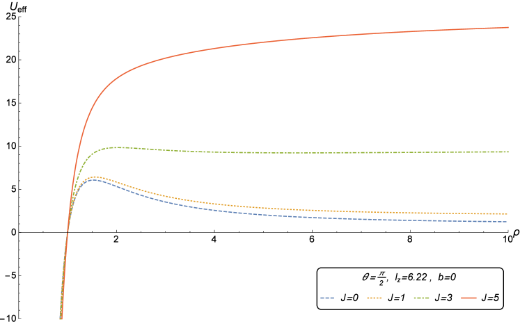
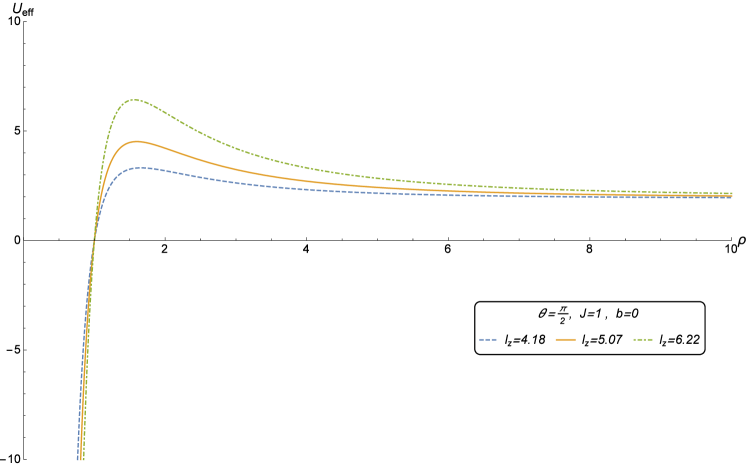
Figure 4: Effective Potential versus $\rho$ in ${\theta=\dfrac{\pi}{2}}$: (a) $b=0$, $l_{z}=6.22$ for $J=0$ (blue dashed), $J=1$ (orange dotted), $J=3$ (green dotdashed), $J=5$ (red line), (b) $b=0$, $J=1$ for $l_{z}=4.18$ (blue dashed), $l_{z}=5.07$ (orange line), $l_{z}=6.22$ (green dotdashed)

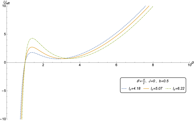
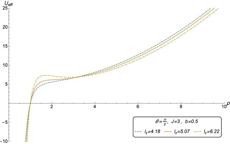
Figure 5: Effective Potential versus $\rho$ in ${\theta=\dfrac{\pi}{2}}$:(a) $J=0$, $b=0.5$ for $l_{z}=4.18$ (blue dashed), $l_{z}=5.07$ (orange line), $l_{z}=6.22$ (green dotdashed),(b) $J=3$, $b=0.5$ for $l_{z}=4.18$ (blue dashed), $l_{z}=5.07$ (orange line), $l_{z}=6.22$ (green dotdashed).

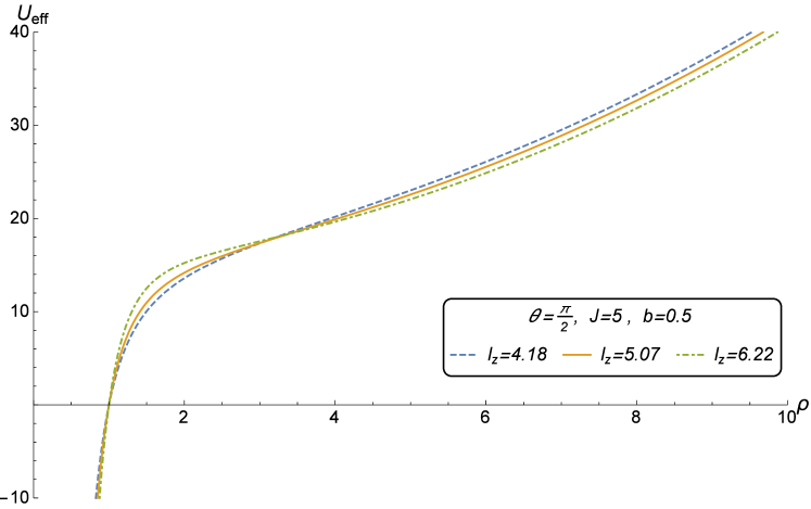
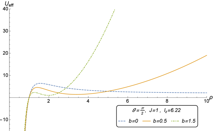
Figure 6: Effective Potential versus $\rho$ in ${\theta=\dfrac{\pi}{2}}$:(a) $J=5$, $b=0.5$ for $l_{z}=4.18$ (blue dashed), $l_{z}=5.07$ (orange line), $l_{z}=6.22$ (green dotdashed), (b) $J=1$, $l_{z}=6.22$ for $b=0$ (blue dashed), $b=0.5$ (orange line), $b=1.5$ (green dotdashed).

Fig.4, Fig.5, and Fig.6 demonstrate the profile of effective potential versus ${\rho}$ in ${\theta=\dfrac{\pi}{2}}$ plane for different ${J}$, ${b}$, and ${l_{z}}$. As it shows here and from Fig.2, one can see that the presence of a magnetic field has a noticeable effect on the shape of potential especially in ${\theta}=\dfrac{\pi}{2}$. The magnitude of ${J}$ has an important effect on it, as well. Fig.4 shows that, for a fixed ${l_{z}=6.22}$, in the absence of a magnetic field, there is no stable circular orbit, which is similar to a five-dimensional black hole in the absence of a magnetic field as mentioned before Kaya:2007kh , and by increasing ${J}$ one can see how the shape of potential changes to a slight line out of the event horizon. According to Eq.(28), the magnitude of potential in larger distances is constant and equal to $(1+J^{2})$ that shows the effects of the extra dimension on the potential in the absence of a magnetic field. Fig.4 illustrates the effects of the changes of ${l_{z}}$ on the shape of the potential, in the absence of a magnetic field and a fixed ${J=1}$.

In Fig.5, Fig.5 and Fig.6, comparing the green lines (with similar ${l_{z}}$) one can see that by increasing the $J$ for fixed $b=0.5$, the shape of potential changes, the distance between maximum and minimum of potential decreases, and the saddle point disappears. This shows the effect of extra dimension (via $J$) on the chance of existence of ISCO. The more the magnitude of $J$, the less the chance of existence of ISCO. In addition, Fig.6 displays that for the large values of $J$, $J=5$ as a sample case, even with a different $l_{z}$, there is no stable circular orbits. But, as it is shown in Fig.6, for the proper amount of $J$ and $l_{z}$ in $b\neq 0$, the potential of black string has ISCO (inflection point in potential). As it is obvious from Fig.4, in the absence of a magnetic field and in large distances from black string ($\rho\rightarrow\infty$) the effective potential is almost constant and its magnitude depends on $J$. According to Eq.(28), this magnitude is ($1+J^{2}$). However, in the presence of the magnetic field, Fig.5 and Fig.6 show a divergent behaviour of the effective potential in large distances ($\rho\rightarrow\infty\Longrightarrow U_{eff}\rightarrow\infty$). In both cases (in the absence and presence of the magnetic field), the effective potential is zero at the event horizon ($\rho=1$), which is obvious from Eq.(28). Besides, the calculated radius of ISCO ($\rho_{0}=3$), shows itself in Fig.6 as an inflection point in the effective potential.

V effective force

One could compute the effective force related to the effective potential by:

$$\vec{F}_{eff}=-\vec{\nabla}U_{eff},$$ (45)

So:

$$F_{\rho}=\dfrac{l_{z}^{2}(2\rho-3)}{\rho^{4}\sin^{2}\theta}+\dfrac{2bl_{z}}{\rho^{2}}-\dfrac{1+J^{2}}{\rho^{2}}-b^{2}(2\rho-1)\sin^{2}\theta,$$ (46)

and

$$F_{\theta}=-(\rho-1)b^{2}\sin(2\theta)+\dfrac{2l_{z}^{2}\cot\theta}{\rho^{4}\sin^{2}\theta}(\rho-1).$$ (47)

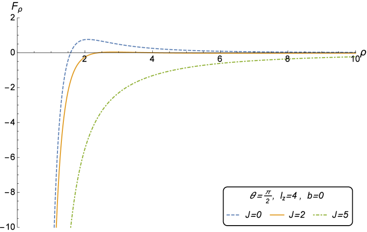
(a)

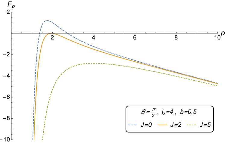
(b)

Figure 7: Effective Force $F_{\rho}$ versus $\rho$ in $l_{z}=4$: (a) for $b=0$, $\theta=\dfrac{\pi}{2}$ and for different $J$, $J=0$ (blue dashed), $J=2$ (orange line), $J=5$ (green dotdashed), (b) for $b=0.5$, $\theta=\dfrac{\pi}{2}$ and for different $J$, $J=0$ (blue dashed), $J=2$ (orange line), $J=5$ (green dotdashed).

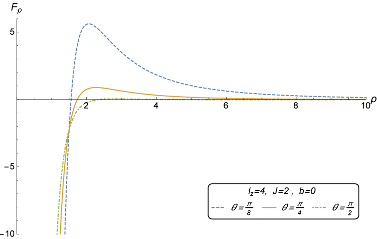
(a)

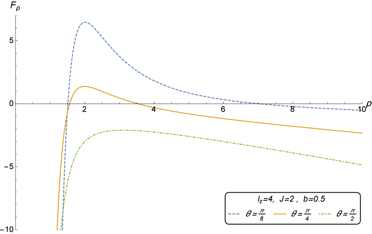
(b)

Figure 8: Effective Force $F_{\rho}$ versus $\rho$in $l_{z}=4$: (a) for $b=0$ in different $\theta$, $\theta=\dfrac{\pi}{8}$ (blue dashed), $\theta=\dfrac{\pi}{4}$ (orange line), $\theta=\dfrac{\pi}{2}$ (green dotdashed), (b) for $b=0.5$ in different $\theta$, $\theta=\dfrac{\pi}{8}$ (blue dashed), $\theta=\dfrac{\pi}{4}$ (orange line), $\theta=\dfrac{\pi}{2}$ (green dotdashed).

In these results, the new constant of motion only appears in $F_{\rho}$ and has no effects on $F_{\theta}$. Also, the new constant of motion $J$ does not couple with the magnetic field. Eq.(46) shows that for the fixed positive $b$ and $l_{z}$, and for distances $\rho\geqslant 1.5$, the first and the second terms in $F_{\rho}$ are positive. It indicates that $l_{z}$ plays a repulsive role in distances larger than $1.5$, while the third term, in which appeared the role of extra dimension, is always negative in all distances and indicates that the extra dimension has strengthened the attraction role in $F_{\rho}$. Moreover, the last term, which displays the second contribution of the magnetic field, is negative for $\rho\geqslant 0.5$. Overall, one can see that always in large distances, $l_{z}$ has a repulsive effect and $J$ has an attractive effect in $F_{\rho}$. In other words, $J$ can be considered as a source of ”extra gravity”. The combination effects of all terms of $F_{\rho}$ is shown in Fig.7(a) and Fig.7(b) in the absence and presence of the magnetic field. Fig.8(b) displays that in $\theta=\dfrac{\pi}{2}$ the attractive components of force are dominant in all distances, but for smaller $\theta$ the repulsive components are dominant in some distances. Fig.7(a) and Fig.8(a) illustrate how the absence of magnetic terms impact on $F_{\rho}$. At the horizon ($\rho=1$), the $F_{\rho}$ is equal to $-[(l_{z}-b)^{2}+1+J^{2}]$. So, the magnitude of $F_{\rho}$ at the horizon depends on the $b$, $l_{z}$ and $J$, but the result is always negative. Therefore, the massive particle at the horizon feels an attractive force along $\rho$, in both the presence and absence of the magnetic field (Fig.7(a) and Fig.7(b)). In large distances from the black string and in the absence of a magnetic field, $F_{\rho}$ tends to zero ($\rho\rightarrow\infty\Longrightarrow F_{\rho}\rightarrow 0$) and the massive particle does not feel any forces along $\rho$ (Fig.7(a)). However, in the presence of the magnetic field and in large distances, $F_{\rho}\rightarrow-b^{2}(2\rho-1)$ which is always attractive and only depends on the magnitude of the magnetic field (Fig.7(b)). Overall, in the defined situation, the interesting point is that increasing the magnitude of $J$, decreases the radial interval in which the $F_{\rho}$ is positive (repulsive radial force). For instance, for $l_{z}=4$ and $J\geqslant 2$ there is no area in which $F_{\rho}\geqslant 0$ ( Fig.7(a) and Fig.7(b)).

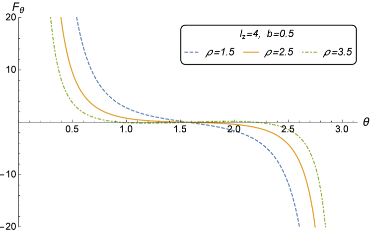
(a)

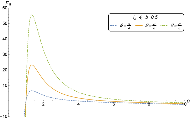
(b)

Figure 9: (a) Effective Force $F_{\theta}$ versus $\theta$, (b) Effective Force $F_{\theta}$ versus $\rho$

On the other hand, the polar component of effective force has different features as follows: Firstly, as mentioned before, this component ($F_{\theta}$) is independent of $J$. Secondly, since $b$ is supposed to be small and it appears in the second order, the impact of a magnetic field on this component is really small and negligible. As it is obvious from Eq.(47) and Fig.9(a), for $\rho\geqslant 1$ and $0\leqslant\theta\leqslant\dfrac{\pi}{2}$, $F_{\theta}$ is always repulsive (the first term in Eq.(47) is not large enough to affect), and in the lower hemisphere ($\dfrac{\pi}{2}\leqslant\theta\leqslant\pi$) it is always attractive. The relation between $F_{\theta}$ and $\rho$ is also interesting. There is always a distance in the range of $1\leqslant\rho\leqslant 1.5$ in which the $F_{\theta}$ has its maximum while decreasing the $\theta$ increases the amount of this maximum. By the way, the suitable situation for investigation of the particle motion is in the equatorial plane $(\theta=\frac{\pi}{2})$ in which this component of force is zero. So, considering these features and since in $\theta=\dfrac{\pi}{2}$ the $F_{\theta}$ is zero, we chose $\theta=\dfrac{\pi}{2}$ plane to investigate the escape velocity in the next section.

VI Escape Velocity

To find the escape velocity of a massive test particle which is moving in the equatorial plane $(\theta_{0}=\frac{\pi}{2})$, the collision between this particle and a particle that comes from infinity is considered. After such a collision, the plane of the first particle will tilt to $(\theta)$ plane. There are three possible statuses, which depend on the mechanism of the collision Zahrani:2013up . When the transferred energy and momentum are small, the orbit will perturb a little (bounded motion). However, if the difference between the new and old total energy is large, the particle can escape to infinity or fall into the black string. To simplify the situation, following assumptions will be considered Frolov:2010mi , Zahrani:2013up :

1. The initial radial velocity of the particle does not change $(\dot{\rho}_{0}=\acute{\dot{\rho}}=0)$.
2. The azimuthal angular momentum does not changed either,

$$l_{z}=l_{z0}=l,$$ (48)

and the total angular momentum is Zahrani:2013up :

$$\textbf{l}^{2}\equiv\rho^{4}\dot{\theta}^{2}+\dfrac{l_{z}^{2}}{\sin^{2}\theta}=\rho^{2}v_{\bot}^{2}+\dfrac{l_{z}^{2}}{\sin^{2}\theta}.$$ (49)

Since the total angular momentum changes and it is assumed that azimuthal angular momentum does not change, the particle gains a new component of velocity which is orthogonal to the equatorial plane, $v_{\bot}\equiv-\rho\dot{\theta}$ Zahrani:2013up . If the particle’s energy after collision is larger than the effective potential at infinity ($\varepsilon_{new}^{2}\geqslant 1+J^{2}$), the escape condition will be satisfied and the particle will escape to infinity ($v_{\bot}\rightarrow v_{esc}$).

Our additional assumption in five dimensions is:

3. The new constant of motion, the angular momentum related to the fifth dimension is constant as well.

By using the first condition and putting the others in that, one can find the escape velocities of neutral and charged particles.

VI.1 Neutral Particles

Hence, for a neutral particle, by considering $b=0$ in Eq. (27) and Eq. (28), we find:

$$\varepsilon_{new}^{2}=\varepsilon_{0}^{2}+(1-\frac{1}{\rho_{0}})v_{\perp}^{2},$$ (50)

in which:

$$\varepsilon_{0}^{2}=(\frac{d\rho_{0}}{d\sigma})^{2}+U_{eff},$$ (51)

$$U_{eff(\rho_{0})}=(1-\frac{1}{\rho_{0}})[\frac{l^{2}}{\rho_{0}^{2}}+1+J^{2}],$$ (52)

so:

$$v_{\perp}=[\frac{\varepsilon_{new}^{2}}{(1-\frac{1}{\rho_{0}})}-(\frac{l^{2}}{\rho_{0}^{2}}+1+J^{2})]^{\frac{1}{2}},$$ (53)

By imposing the escape condition:

$$v_{esc}\geqslant[\frac{\varepsilon_{new}^{2}}{(1-\frac{1}{\rho_{0}})}-(\frac{l^{2}}{\rho_{0}^{2}}+1+J^{2})]^{\frac{1}{2}},$$ (54)

in which:

$$\varepsilon_{new}^{2}\geqslant 1+J^{2},$$ (55)

According to Eq. (39) and Eq. (40), the escape velocity for a particle in ISCO is:

$$v_{esc(ISCO)}\geqslant\sqrt{\frac{1+J^{2}}{6}},$$ (56)

which only depends on the $J$. In the case of $(w=0\rightarrow J=0)$, these results are similar to the results of Frolov:2010mi , Majeed:2014kka , and Zahrani:2013up for Schwarzschild black hole. In the asymptotic limit, $\varepsilon_{new}^{2}\rightarrow 1+J^{2}$ Majeed:2014kka obtains:

$$v_{esc}=[\frac{1+J^{2}}{(1-\frac{1}{\rho_{0}})}-(\frac{l^{2}}{\rho_{0}^{2}}+1+J^{2})]^{\frac{1}{2}}.$$ (57)

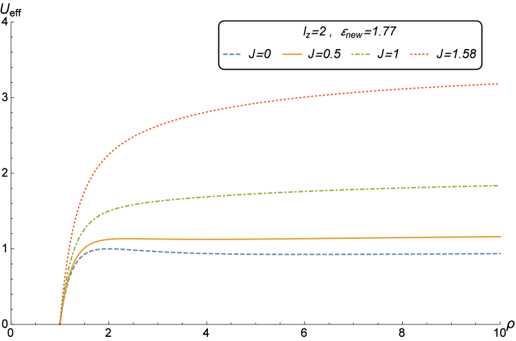
(a)

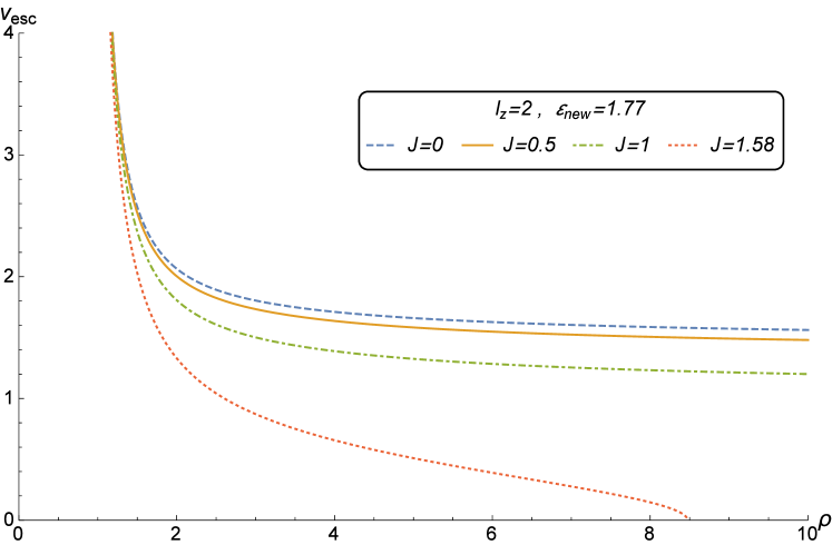
(b)

Figure 10: Effective Potential and Escape Velocity versus $\rho$ for a neutral particle and $l_{z}=2$, $\varepsilon_{new}=1.77$ in $J=0$ (blue dashed), $J=0.5$ (orange line), $J=1$ (green dotdashed), $J=1.58$ (red dotted)

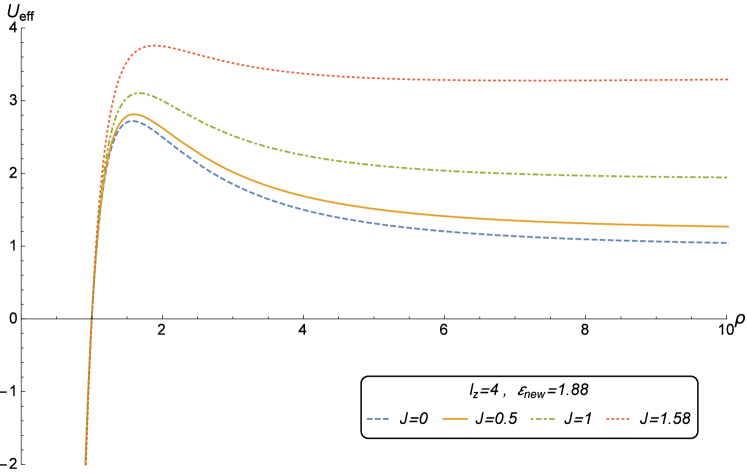
(a)

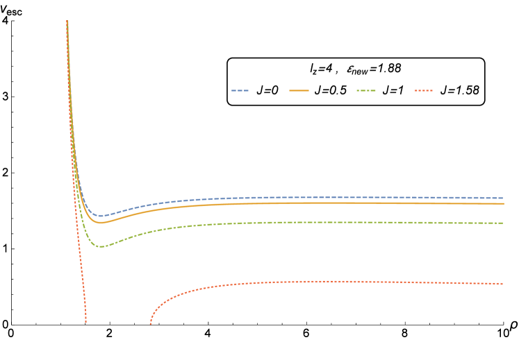
(b)

Figure 11: Effective Potential and Escape Velocity versus $\rho$ for a neutral particle and $l_{z}=4$, $\varepsilon_{new}=1.88$ in $J=0$ (blue dashed), $J=0.5$ (orange line), $J=1$ (green dotdashed), $J=1.58$ (red dotted)

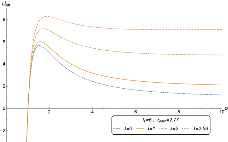
(a)

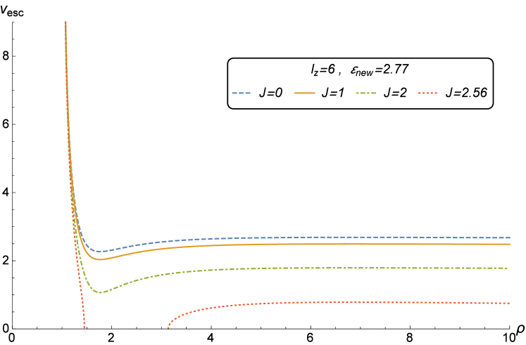
(b)

Figure 12: Effective Potential and Escape Velocity versus $\rho$ for a neutral particle and $l_{z}=6$, $\varepsilon_{new}=2.77$ in $J=0$ (blue dashed), $J=1$ (orange line), $J=2$ (green datdashed), $J=2.56$ (red dotted).

Fig.10, Fig.11, and Fig.12 show the relation between the escape velocity and the dimensionless distance from the center of the black string and their relevant potential for each case. According to Eq. (54) and as Fig.11 and Fig.12 illustrate, the extra dimension shows its effects in increasing the threshold of escape velocity in all distances. Besides, in the large distances the escape velocity is constant and comes from $\rho_{0}\rightarrow\infty$ in Eq. (54). So, the constant magnitude of escape velocity in the large distance is $(\varepsilon_{new}^{2}-1-J^{2})^{1/2}$. Near the event horizon ($\rho\rightarrow 1$), the escape velocity tends to infinity ($v_{esc}\rightarrow+\infty$) which is expected (Fig.10(b), Fig.11(b) and Fig.12(b)).

Also, Fig.10(b) illustrates that for a small amount of $l$ and a proper amount of $\varepsilon_{new}$, the escape velocity decreases by the distance, which comes from the result of. Also, as it has been shown in Fig.11(b) and Fig.12(b), for large enough amounts of $l$ and the proper amount of $\varepsilon_{new}$, there exists a suitable $J$ (completely dependent on $\varepsilon_{new}$ by $\varepsilon_{new}^{2}\approx 1+J^{2}$.) that vanishes the escape velocity in some distance which means there is a balance between attractive and repulsive forces. Moreover, as it is shown in Fig.11(b) and Fig.12(b), increasing the amount of $l$ causes this special amount of $J$ to increase and also makes this distance to be closer to the center of the black string. In addition, it is obvious from Eq. (54) that in $J=0$ (Schwarzschild black hole) such point does not exist in finite distances, as it has been shown in Fig.11(b) and Fig.12(b).

VI.2 Charged Particles

In the case of a charged particle, the situation is much more complicated. In general by using all assumptions and by considering Eq. (27) and Eq. (28), the result is:

$$v_{\bot}^{2}=\dfrac{\varepsilon_{new}^{2}}{(1-\frac{1}{\rho_{0}})}-1-J^{2}+2bl-\dfrac{l^{2}}{\rho_{0}^{2}\sin^{2}\theta}-b^{2}\rho_{0}^{2}\sin^{2}\theta,$$ (58)

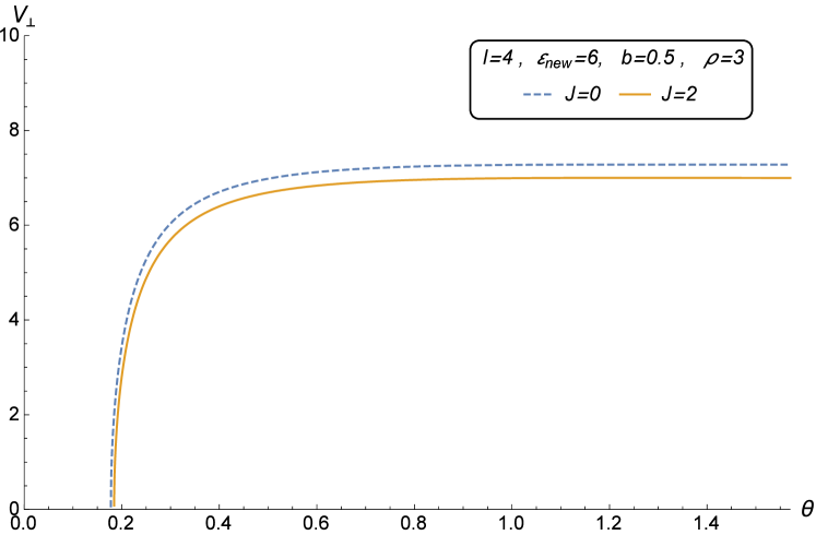
(a)

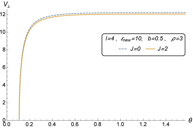
(b)

Figure 13: $v_{\bot}$ versus $\theta$ for a charged particle in $l=4$, $b=0.5$, $\rho=3$: (a) $\varepsilon_{new}=6$: $J=0$ (blue dashed), $J=2$ (orange line), (b) $\varepsilon_{new}=10$: $J=0$ (blue dashed), $J=2$ (orange line).

in which $\rho_{0}$ is the distance from the center of the black string that according to the first assumption it does not change, and the plane of particles tilts to $\theta$ after collision. So, one can see that the result for a charged particle in a black string is different from a black hole only in the existence of $J^{2}$ in Eq. (58). Fig.13 illustrates the impact of $J$ on $v_{\bot}$. At the very first moment after collision $\theta$ is $\dfrac{\pi}{2}$, so $v_{\bot}$ of a charged particle obtains from:

$$v_{\bot}=\sqrt{\dfrac{\varepsilon_{new}^{2}}{(1-\frac{1}{\rho_{0}})}-1-J^{2}+2bl-\dfrac{l^{2}}{\rho_{0}^{2}}-b^{2}\rho_{0}^{2}},$$ (59)

which for $J=0$, is in accordance with Jamil:2014rsa .

VII Motion and trajectories of particles

In this section, we will discuss the analytical solutions of the equations of motion and plot some possible orbits for massive particles in the black string space-time. We rewrite Eqs. 6 and 19 using Eq.24 and the Mino time ($\rho^{2}d\gamma=d\sigma$)Mino:2003yg , Grunau:2013oca as follows:

$$(\dfrac{d\rho}{d\gamma})^{2}=(\varepsilon^{2}-J^{2}-1)\rho^{4}+(J^{2}+1)\rho^{3}-l^{2}(\rho^{2}-\rho),$$ (60)

$$(\dfrac{d\rho}{d\gamma})^{2}=-b^{2}\rho^{6}+b^{2}\rho^{5}+(\varepsilon^{2}-J^{2}+2lb-1)\rho^{4}+(J^{2}-2lb+1)\rho^{3}-l^{2}(\rho^{2}-\rho).$$ (61)

elliptic function

Eq. (60) and Eq. (61) for $b^{2}=0$, are polynomials of degree four as $(\dfrac{d\rho}{d\gamma})^{2}=\sum_{i=0}^{4}c_{i}\rho^{i}$, and by substitution $\rho=\frac{1}{u}+\rho_{R}$, can be convert to a polynomial of degree three as:

$$(\frac{du}{d\gamma})^{2}=\sum_{j=1}^{3}a_{j}u^{j},\;\;\;\;\;u(\gamma_{0})=u_{0},$$ (62)

where $\rho_{R}$ is a zero of $R$ and:

$$a_{j}=\frac{1}{(4-j)!}\frac{d^{(4-j)}R}{d\tilde{r}^{4-j}}(\gamma_{R}),$$ (63)

Again by substitution $u=\frac{1}{a_{3}}(4y-\frac{a_{2}}{3})$, Eq.(62), transforms to an elliptical type differential equation, known as the Weierstrass form as Hackmann:2008zz ; Soroushfar:2015wqa ; Soroushfar:2016esy :

$$(\frac{dy}{d\gamma})^{2}=4y^{3}-g_{2}y-g_{3}=p_{3}(y),$$ (64)

with the Weierstrass invariants:

$$g_{2}=\frac{1}{16}(\frac{4}{3}a_{2}^{2}-4a_{1}a_{3}),\;\;\;g_{3}=\frac{1}{16}(\frac{1}{3}a_{1}a_{2}a_{3}-\frac{2}{27}a_{2}^{3}a_{3}^{2}).$$ (65)

Therefore, the solution of Eq. (64), using the Weierstrass function, is:

$$y(\gamma)=\wp(\gamma-\gamma_{in};g_{2},g_{3}),$$ (66)

in which $\gamma_{in}=\gamma_{0}+\int_{y_{0}}^{\infty}\frac{dy}{\sqrt{4y^{3}-g_{2}y-g_{3}}}$ with $\gamma_{0}=\frac{1}{4}(\frac{a_{3}}{\rho_{0}-\rho_{R}}+\frac{a_{2}}{3})$ depends only on the initial value $\gamma_{0}$ and $\rho_{0}$. As a result, the solution of polynomials of degree four (Eq. (60) and Eq. (61) for $b^{2}=0$) is

$$\rho(\gamma)=\frac{a_{3}}{4\wp(\gamma-\gamma_{in};g_{2},g_{3})-\frac{a_{2}}{3}}+\rho_{R}.$$ (67)

hyper-elliptic function

Eq. (61) is a polynomial of degree six as $(\dfrac{d\rho}{d\gamma})^{2}=\sum_{i=0}^{6}c_{i}\rho^{i}$, which by substitution $\rho=\frac{1}{y}+\rho_{R}$, transforms to a polynomial of degree five as:

$$\left(\frac{dy}{d\gamma}\right)^{2}=P_{5}(y)=\sum_{i=0}^{5}a_{i}\rho^{i}.$$ (68)

The above equation is of a hyper-elliptic type, and so its analytic solution can be written in the form of derivatives of the Kleinian $\sigma$ function as Soroushfar:2016esy , Hackmann:2008zz , Enolski:2010if :

$$y(\gamma)=-\frac{\sigma_{1}(\gamma_{\infty})}{\sigma_{2}(\gamma_{\infty})}|_{\sigma(\gamma_{\infty})=0},$$ (69)

where $\gamma_{\infty}=(\gamma_{2},\gamma-\gamma^{{}^{\prime}}_{in})$, $\gamma^{{}^{\prime}}_{in}=\gamma_{in}+\int_{\gamma_{in}}^{\infty}\frac{ydy^{{}^{\prime}}}{\sqrt{P_{5}(y^{{}^{\prime}})}}$, and $\gamma_{2}$ is determined by the condition $\sigma(\gamma_{\infty})=0$. The other component in Eq. (69) is the function $\sigma_{i}$ which is the ith derivative of Kleinian $\sigma$ function and $\sigma_{z}$ is:

$$\sigma_{z}=Ce^{zt}kz\theta[g,\theta](2w^{-1}z;T),$$ (70)

in which $T$ is the symmetric Riemann matrix, $C$ is a constant, $\theta$ is the Riemann function with characteristic $[g,h]$ which $2[g,h]=(0,1)^{t}+(1,1)^{t}T$, $\omega$ is the period matrix, $k=\eta(2)^{-1}$ in which $\eta$ is the periodmatrix of the second kind, therefore the solution of polynomials of degree six (Eq. (61)) is:

$$\rho(\gamma)=-\frac{\sigma_{2}(\gamma_{\infty})}{\sigma_{1}(\gamma_{\infty})}.$$ (71)

Trajectory

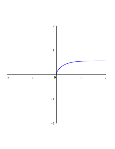
(a) TO with parameters $L=2$, $E=2$, $b=0$, $J=0.5$, $a_{2}=-4$, $a_{3}=4$, $g_{2}=0.08$, $g_{3}=-2.87$ .

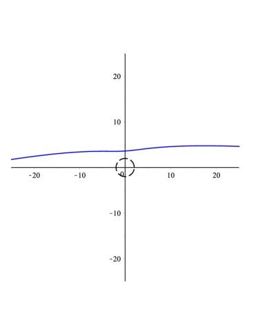
(b) EO with parameters $L=2.24$, $E=1$, $b=0$, $J=0$, $a_{2}=-5$, $a_{3}=5$, $g_{2}=0.84$, $g_{3}=0.06$ .

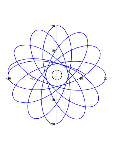
(c) BO with parameters $L=2.24$, $E=1$, $b=0$, $J=0.2$, $a_{2}=-5$, $a_{3}=5$, $g_{2}=0.79$, $g_{3}=0.1$.

Figure 14: Three $xy$ plane plots of particle orbits in the black string space-time in the absence of a magnetic field. The black dashed circle depicts the position of the horizon and the blue curves indicate the orbits.

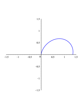
(a) TO with parameters $L=3$, $E=1.25$, $b=0.01$, $J=0$, $a_{2}=-9$, $a_{3}=9$, $g_{2}=4.54$, $g_{3}=-1.22$.

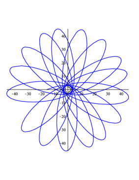
(b) BO with parameters $L=2$, $E=0.97$, $b=0.01$, $J=0$, $a_{2}=-4$, $a_{3}=4$, $g_{2}=0.37$, $g_{3}=-0.0046$.

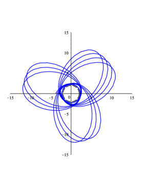
(c) BO with parameters $L=1.87$, $E=0.97$, $b=0.01$, $J=0.2$, $a_{2}=-3.5$, $a_{3}=3.5$, $g_{2}=0.14$, $g_{3}=-0.01$.

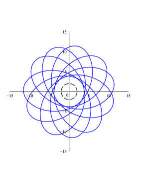
(d) BO with parameters $L=2$, $E=0.97$, $b=0.01$, $J=0.2$, $a_{2}=-4$, $a_{3}=4$, $g_{2}=0.33$, $g_{3}=0.022$.

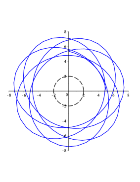
(e) BO with parameters $L=2$, $E=0.97$, $b=0.006$, $J=0.2$, $a_{2}=-4$, $a_{3}=4$, $g_{2}=0.317$, $g_{3}=0.032$.

Figure 15: Five $xy$ plane plots of particle orbits in the black string space-time in presence of a magnetic field. The black dashed circle depict the position of the horizon and the blue curves indicate the orbits.

With these analytical results, we find some possible orbits for particles in the black string space-time. Depending on $b$, $J$, $\varepsilon$ and $l$ parameters, $Terminating$ $orbit$ (TO), $Escape$ $orbit$ (EO) and $Bound$ $orbit$ (BO) are possible. Examples of such particle orbits in the black string space-time in the absence and in the presence of a magnetic field, are shown in Figs. 14, and 15 respectively. It can be seen from Fig. 14 that, in the absence of magnetic field, TO, BO and EO are possible, where increasing the value of $J$, may change an escape orbit to a bound orbit. While in the presence of magnetic field, in which both BO and TO are possible (as depicted in Fig. 15) increasing the value of $J$, appears as decreasing the radius of the bound orbit.

VIII Conclusion

We studied some dynamical properties of neutral and charged particles around a simple and weakly magnetized black string and the attributes of their escape velocity. The results are:

i. Adding an extra dimension has a slight influence on the effective potential, but the magnitude of the new constant of motion $(J)$ affects the shape of the potential and thereby the chance of existence of the stable circular orbits.

ii. In the calculation of ISCO’s parameters, up to the first order of perturbation, due to the presence of a magnetic field, the radius of ISCO is independent of the magnetic field and $J$, also the solution resembles Schwarzschild black hole. But, $l_{zISCO}$ and $\varepsilon_{ISCO}$ are related to $J$ even before the perturbation.

iii. We also calculated the components of the effective force. The new constant of motion related to the new dimension, adds a pure attractive term on $F_{\rho}$. But it does not have any effects on the other component of the effective force.

iv. Moreover, we calculated the escape velocity of a neutral particle and saw how the magnitude of $J$ would vanish the escape velocity in some $\rho$ for a neutral particle. It does not happen in a Schwarzschild black hole ($J=0$).

v. Finally, we analysed the analytical solutions of the geodesic equations in terms of elliptic and hyperelliptic functions. With these analytical results, we have found some possible orbits for particles in the black string space-time. These orbits illustrate that, independent of the presence or the absence of a magnetic field term, the effect of the fifth dimension, $J$, appears as a source of extra gravity in a planetary motion. In the absence of a magnetic field, TO, BO and EO are possible, while in the presence of a magnetic field, BO and TO are possible.

In conclusion, by comparing a black hole to a black string, we could see that the general form of the effective potential and equations of motion are almost similar, however, in some properties related to the escape velocity of a particle, the magnitude of the new constant of motion causes some differences and even shows the presence of a new term on the effective force.

References

- (1) N. Arkani-Hamed, S. Dimopoulos and G. R. Dvali, Phys. Lett. B 429, 263 (1998)
- (2) I. Antoniadis, N. Arkani-Hamed, S. Dimopoulos and G. R. Dvali, Phys. Lett. B 436, 257 (1998)
- (3) L. Randall and R. Sundrum, Phys. Rev. Lett. 83, 3370 (1999)
- (4) L. Randall and R. Sundrum, Phys. Rev. Lett. 83, 4690 (1999)
- (5) R. Kaya, Gen. Rel. Grav. 39, 211 (2007).
- (6) C. H. Lee, Phys. Rev. D 74, 104016 (2006)
- (7) T. Kaluza, Sitzungsber. Preuss. Akad. Wiss. Berlin (Math. Phys. ) 1921, 966 (1921).
- (8) N. A. Obers, Lect. Notes Phys. 769, 211 (2009)
- (9) J. Kunz, Nucl. Phys. Proc. Suppl. 251-252, 27 (2014).
- (10) B. Kleihaus, J. Kunz and E. Radu, JHEP 0606, 016 (2006)
- (11) N. Kaloper, Phys. Rev. D 48 (1993) 4658
- (12) R. Emparan, G. T. Horowitz and R. C. Myers, JHEP 0001, 021 (2000)
- (13) T. Hirayama and G. Kang, Phys. Rev. D 64, 064010 (2001)
- (14) B. Kleihaus and J. Kunz, “Black Holes in Higher Dimensions (Black Strings and Black Rings),” arXiv:1603.07267 [gr-qc].
- (15) B. Mashhoon, H. Liu and P. Wesson, Phys. Lett. B 331, 305 (1994)
- (16) D. Kalligas, P. S. Wesson and C. W. F. Everitt, Astrophys. J. 439, 548 (1994).
- (17) J. Ponce de Leon and P. S. Wesson, Fields Inst. Commun. 15, 325 (2001).
- (18) S. S. Seahra and P. S. Wesson, Class. Quant. Grav. 20, 1321 (2003)
- (19) P. S. Wesson, B. Mashhoon and H. Liu, Mod. Phys. Lett. A 12, 2309 (1997).
- (20) H. Y. Liu and P. S. Wesson, Class. Quant. Grav. 13, 2311 (1996).
- (21) P. S. Wesson, Observatory 132, 372 (2012)
- (22) P. S. Wesson and J. Ponce de Leon, Class. Quant. Grav. 11, 1341 (1994).
- (23) B. Kleihaus, J. Kunz and F. Navarro-Lerida, AIP Conf. Proc. 977, no. 1, 94 (2008)
- (24) J. Kunz, F. Navarro-Lerida, J. Viebahn and D. Maison, “Charged rotating black holes in higher dimensions”, The Eleventh Marcel Grossmann Meeting, pp. 1400-1402 (2008).
- (25) H. Liu and J. M. Overduin, Astrophys. J. 538, 386 (2000)
- (26) F. Luo and H. Liu, Chin. Phys. Lett. 23, 2903 (2006)
- (27) F. R. Tangherlini, Il Nuovo Cimento (1955-1965). 27, 636(1963)
- (28) Myers, R. C. and Perry, M. J, Annals of Physics, 172, 304 9(1986).
- (29) R. Gregory and R. Laflamme, Phys. Rev. D 37, 305 (1988).
- (30) A. Chodos and S. L. Detweiler, Gen. Rel. Grav. 14, 879 (1982).
- (31) H. C. Kim and J. Lee, Phys. Rev. D 77, 024012 (2008)
- (32) D. Marolf, Phys. Rev. D 71, 127504 (2005)
- (33) G. T. Horowitz and K. Maeda, Phys. Rev. Lett. 87, 131301 (2001)
- (34) V. Lacquaniti, G. Montani, D. Pugliese and R. Ruffini, Gen. Rel. Grav. 43, 1103 (2011)
- (35) P. S. Wesson (1999), Space-Time-Matter(World Scientific Publishing Co. Pte. Ltd, Singapore).
- (36) J. M. Overduin and P. S. Wesson, Phys. Rept. 283, 303 (1997)
- (37) P. S. Wesson and J. M. Overduin(2018), Principles of Space-Time-Matter(Cosmology, Particles and Waves in Five Dimensions).
- (38) S. S. Seahra and P. S. Wesson, Gen. Rel. Grav. 33, 1731 (2001)
- (39) M. Liu, H. Liu, F. luo and L. Xu, Gen. Rel. Grav. 39, 1389 (2007)
- (40) H. Liu and P. S. Wesson, Phys. Lett. B 377, 420 (1996).
- (41) H. Y. Liu and P. S. Wesson, J. Math. Phys. 33, 3888 (1992).
- (42) P. Brax and C. van de Bruck, Class. Quant. Grav. 20, R201 (2003)
- (43) D. Langlois, Prog. Theor. Phys. Suppl. 148, 181 (2003)
- (44) S. Ponglertsakul, P. Burikham and L. Tannukij, Eur. Phys. J. C 78, no. 7, 584 (2018)
- (45) Y. Gim and W. Kim, Phys. Lett. B 791, 390 (2019)
- (46) M. R. Setare and H. Adami, Phys. Rev. D 98, no. 8, 084015 (2018)
- (47) M. Azzola, D. Klemm and M. Rabbiosi, JHEP 1810, 080 (2018)
- (48) L. A. H. Mamani, J. Morgan, A. S. Miranda and V. T. Zanchin, Phys. Rev. D 98, no. 2, 026006 (2018)
- (49) H. L. Dao and P. Karndumri, Eur. Phys. J. C 79, no. 2, 137 (2019)
- (50) T. Nakas, N. Pappas and P. Kanti, Phys. Rev. D 99, no. 12, 124040 (2019)
- (51) A. Giacomini, M. Lagos, J. Oliva and A. Vera, Phys. Rev. D 98, no. 4, 044019 (2018)
- (52) A. Cisterna, C. Corral and S. del Pino, Eur. Phys. J. C 79, no. 5, 400 (2019)
- (53) E. Hackmann, B. Hartmann, C. Laemmerzahl and P. Sirimachan, Phys. Rev. D 81, 064016 (2010)
- (54) V. P. Frolov and A. A. Shoom, Phys. Rev. D 82, 084034 (2010)
- (55) G. Z. Babar, M. Jamil and Y. K. Lim, Int. J. Mod. Phys. D 25, no. 02, 1650024 (2015)
- (56) S. Soroushfar, R. Saffari and A. Jafari, Phys. Rev. D 93, no. 10, 104037 (2016)
- (57) S. Soroushfar, R. Saffari and E. Sahami, Phys. Rev. D 94, no. 2, 024010 (2016)
- (58) B. Majeed, S. Hussain and M. Jamil, Adv. High Energy Phys. 2015, 671259 (2015)
- (59) E. Hackmann, B. Hartmann, C. Lammerzahl and P. Sirimachan, Phys. Rev. D 82, 044024 (2010)
- (60) S. Grunau and B. Khamesra, Phys. Rev. D 87, no. 12, 124019 (2013)
- (61) A. Tursunov, M. Kolo , A. Abdujabbarov, B. Ahmedov and Z. Stuchl k, Phys. Rev. D 88, 124001 (2013)
- (62) K. Akiyama et al. [Event Horizon Telescope Collaboration], Astrophys. J. 875 (2019) no.1, L5.
- (63) R. L. Znajek, Nature. 262, 270 (1976).
- (64) R. D. Blandford and R. L. Znajek, Mon. Not. Roy. Astron. Soc. 179, 433 (1977).
- (65) V. P. Frolov, Phys. Rev. D 85, 024020 (2012)
- (66) R. M. Wald, Phys. Rev. D 10, 1680 (1974).
- (67) A. M. A. Zahrani, V. P. Frolov and A. A. Shoom, Phys. Rev. D 87, no. 8, 084043 (2013)
- (68) A. N. Aliev and N. Ozdemir, Mon. Not. Roy. Astron. Soc. 336, 241 (2002)
- (69) A. W. McDavid and C. D. McMullen, “Generalizing Cross Products and Maxwell’s Equations to Universal Extra Dimensions,” hep-ph/0609260.
- (70) P. I. Jefremov, O. Y. Tsupko and G. S. Bisnovatyi-Kogan, Phys. Rev. D 91, no. 12, 124030 (2015)
- (71) M. Jamil, S. Hussain and B. Majeed, Eur. Phys. J. C 75, no. 1, 24 (2015)
- (72) F. Rahaman, M. Kalam, A. DeBenedictis, A. A. Usmani and S. Ray, Mon. Not. Roy. Astron. Soc. 389, 27 (2008)
- (73) Y. Mino, Phys. Rev. D 67, 084027 (2003)
- (74) E. Hackmann and C. Lammerzahl, Phys. Rev. D 78, 024035 (2008)
- (75) S. Soroushfar, R. Saffari, J. Kunz and C. Lammerzahl, Phys. Rev. D 92, no. 4, 044010 (2015)
- (76) S. Soroushfar, R. Saffari, S. Kazempour, S. Grunau and J. Kunz, Phys. Rev. D 94, no. 2, 024052 (2016)
- (77) V. Z. Enolski, E. Hackmann, V. Kagramanova, J. Kunz and C. Lammerzahl, J. Geom. Phys. 61, 899 (2011)