Device-independent dimension test in a multiparty Bell experiment

Abstract

A device-independent dimension test for a Bell experiment aims to estimate the underlying Hilbert space dimension that is required to produce given measurement statistical data without any other assumptions concerning the quantum apparatus. Previous work mostly deals with the two-party version of this problem. In this paper, we propose a very general and robust approach to test the dimension of any subsystem in a multiparty Bell experiment. Our dimension test stems from the study of a new multiparty scenario which we call prepare-and-distribute. This is like the prepare-and-measure scenario, but the quantum state is sent to multiple, non-communicating parties. Through specific examples, we show that our test results can be tight. Furthermore, we compare the performance of our test to results based on known bipartite tests, and witness remarkable advantage, which indicates that our test is of a true multiparty nature. We conclude by pointing out that with some partial information about the quantum states involved in the experiment, it is possible to learn other interesting properties beyond dimension.

I Introduction

Suppose we have an unknown quantum system and we want to assess its quantum properties. One way to tackle this problem is by using only classical information obtained by interacting with the target system classically and thus no (possibly unrealistic) assumptions need to be made concerning the quantum states and/or measurements involved. For this purpose, often what people do is choose different means/settings to measure the system, then collect the corresponding statistical data, which is of course classical. It is well-known, on the other hand, that if one wants to describe a quantum system completely using only classical information, the amount of information needed will increase exponentially with the size of the quantum system, which is usually much more than what is collected through measurements NC00 . Therefore, it would seem that we cannot infer any useful information about the quantum state using a limited amount of statistical data alone.

Interestingly, these tasks are indeed possible in some cases, and the information inferred is said to be device-independent Ekert91 ; ABM+07 . Clearly, they are attractive not only mathematically, but also from an application standpoint. For example, when a businessman wants to sell a quantum product, it would help if he can convince potential clients that the product is behaving as advertised. Instead of taking the machine apart piece by piece and trying to convince the buyer that there is nothing funny going on, e.g., something maliciously entangled with his company laboratory, he can choose to interact with it via measurements to obtain a small number of outcome statistics, and invoke device-independent results from the literature.

Bell experiments are typical settings to demonstrate phenomena of device-independence BPA+08 . In such a setting, a number of spatially separated parties share a quantum state and each party chooses one local measurement from a finite selection to measure his/her subsystem. The statistical data for all possible choices of measurements is recorded as a correlation. For bipartite cases of Bell experiments, it has been shown that the dimension of each party can be estimated in a device-independent manner BPA+08 ; SVV15 (see also WCD08 ). This problem is motivated as follows. It is well-known that Hilbert space dimension is a valuable resource in quantum processing tasks. Therefore, for any quantum correlation that is generated in a quantum setting, we often prefer the dimension required to produce this correlation to be as small as possible. Thus, being able to estimate the underlying Hilbert space dimension device-independently is very useful.

In particular, to solve this fundamental problem, using the fact that some entangled quantum states can produce correlations violating certain Bell inequalities Bell64 , the concept of dimension witness was proposed to estimate the underlying dimension, where the key idea is to build a relation between dimension and the extent that Bell inequalities are violated BPA+08 . The approach of dimension witness requires sets of quantum correlations to be convex, thus shared classical randomness is assumed. This approach is powerful, but it relies heavily on the availability of a Bell inequality for the statistics being tested. Assuming that shared classical randomness is not a free resource, i.e., it is absorbed into the entangled quantum state, a new easy-to-compute dimension bound for this problem has also been provided SVV15 . This bound is independent of any Bell inequalities, and thus it is very convenient to use as it can be readily applied to any correlation data. Recently, the approach of SVV15 was used to certify system dimensionality in a newly proposed experimental platform for multidimensional quantum systems WPD+18 . Other examples of device-independence on Bell experiments include assessing the amount of entanglement in some bipartite cases MBL+13 , and even pinning down the underlying quantum states completely, a task known as self-testing PR92 ; BMR92 ; MY98 ; MY04 ; CGS17 .

Though more than one approach has been discovered to deal with device-independent dimension estimation of bipartite Bell experiments, multipartite versions have not been found to the best of our knowledge. This problem is not only important and realistic, but also interesting in its own right as the generalization from bipartite to multipartite cases enriches the mathematics needed considerably as it is much more complicated. However, using the standard approach of finding dimension witnesses based on Bell inequalities to address this problem is a very difficult task as this requires much knowledge of the complicated structures of multipartite quantum correlations. Indeed, Bell inequalities in the multiparty setting are very hard to find and are not that well understood Svetlichny87 ; CGP+02 , especially compared to the two-party case. To get around these difficulties, in this paper we develop a general technique for this problem which results in an easy-to-compute lower bound for the underlying dimension of any subsystem in a general multiparty Bell experiment. To this end, we define a multiparty quantum scenario called prepare-and-distribute, and then propose an efficient way to estimate the distances between quantum states in this scenario based on measurement statistical data only. This allows us to identify device-independently a desired lower bound for the target dimension in the multipartite Bell setting. Through specific examples, we show that our result can be tight. At the same time, since we are interested in the dimensions of individual parties, in principle we can also use methods for bipartite cases (e.g. in Ref. SVV15 ) to tackle our problem. By a concrete example, we illustrate that our new result in this paper is much better than generalizations from known bipartite results. This demonstrates that it is of a true multiparty nature. We also point out that with more information on the target quantum state, it is possible to learn other quantum properties beyond dimension in some circumstances.

II Preliminaries

II.1 Multiparty Bell Scenario

In a multiparty Bell scenario, we have $k+1$ physically separated parties, sharing a quantum state $\rho$ acting on a $(k+1)$-partite Hilbert space $\bigotimes_{i=1}^{k+1}\mathbb{C}^{d_{i}}$, where $d_{i}$ is the dimension of the $i$-th subsystem. Each party has a local measurement apparatus, which allows for various measurement settings which can be applied to their subsystems.

As not to be bound to $26$ parties, we shall call one of them Alice, and the rest of the parties Bob-$1$, Bob-$2$, up to Bob-$k$. Alice will have measurement settings given by a finite set $X$ and Bob-$j$ will have measurement settings from a finite set $Y_{j}$. Thus, when they measure the shared quantum state $\rho$ with their chosen settings, the probability that Alice gets outcome $a$ (from a finite set $A$) and Bob-$j$ gets outcome $b_{j}$ (from a finite set $B_{j}$) is given by

$$p(ab_{1}\cdots b_{k}|xy_{1}\cdots y_{k})=\mathrm{Tr}\left(\left(M^{x}_{a}\otimes\bigotimes_{j=1}^{k}(N^{j})^{y_{j}}_{b_{j}}\right)\rho\right),$$ (1)

where $\{M^{x}_{a}:a\in A\}$ is Alice’s local positive-operator valued measure (POVM) and $\{(N^{j})^{y_{j}}_{b_{j}}:b_{j}\in B_{j}\}$ is Bob-$j$’s local POVM. A three-party Bell experiment is illustrated in FIG. 1. The set of all joint conditional probabilities $p(ab_{1}\cdots b_{k}|xy_{1}\cdots y_{k})$ is called a $(k+1)$-correlation (or just correlation when $k$ is clear from context).

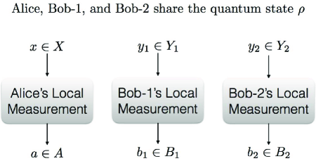
Figure 1: Alice, Bob-$1$, and Bob-$2$ in a three-party Bell experiment.

II.2 The prepare-and-distribute scenario

We now define a new $(k+1)$-party quantum scenario that is useful for the purposes of this paper. Suppose a single party, say Paula, prepares a $k$-partite quantum state $\rho_{x}$, for some $x\in X$, and distributes it to $k$ different, physically separated parties, which we call Roger-$1$, …, Roger-$k$. Then Roger-$j$ measures his corresponding subsystem with available local POVM indexed by $y_{j}$ and gets the outcome $b_{j}$. The measurement settings and outcomes share the same notation as in the previous discussion about multiparty Bell experiments for reasons that will be clear shortly. Like a $(k+1)$-party Bell correlation, a prepare-and-distribute correlation can be defined as below with similar notations,

$$p(b_{1}\cdots b_{k}|xy_{1}\cdots y_{k})=\mathrm{Tr}\left(\bigotimes_{j=1}^{k}(N^{j})^{y_{j}}_{b_{j}}\ \rho_{x}\right).$$ (2)

A prepare-and-distribute experiment involving three parties can be seen in FIG. 2. Later we will discuss the close relationship between multiparty Bell scenarios and prepare-and-distribute scenarios.

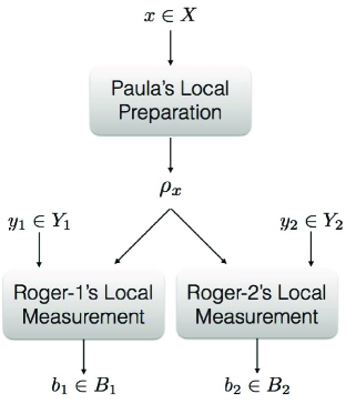
Figure 2: Paula, Roger-$1$, and Roger-$2$ in a three-party prepare-and-distribute experiment.

III Main results

III.1 Bounding distances between quantum states in a prepare-and-distribute scenario

In this subsection, we consider the following problem: Suppose we are given a prepare-and-distribute setting and the corresponding correlation data $p(b_{1}\cdots b_{k}|xy_{1}\cdots y_{k})$, can we give a nontrivial estimation for the distance between two arbitrary preparations $\rho_{x}$ and $\rho_{x^{\prime}}$? The answer is affirmative.

In this paper, we choose the concept of fidelity to measure the distances between quantum states NC00 . For two quantum states $\sigma_{1}$ and $\sigma_{2}$ acting on the same Hilbert space, their fidelity is defined as $\mbox{\bf F}(\sigma_{1},\sigma_{2})=\|\sqrt{\sigma_{1}}\sqrt{\sigma_{2}}\|_{1}$. A useful property of fidelity is that for any two quantum states, if one measures them using the same measurement, then the fidelity between the two outcome distributions (as classical-quantum states) is no less than that between the two original quantum states NC00 . Therefore, by compositing all the local POVMs on Rogers as a whole, we can immediately get an upper bound for $\mbox{\bf F}(\rho_{x},\rho_{x^{\prime}})$ as below:

$$\!\!\!\!\!\!\!\!\sum_{b_{1}\cdots b_{k}}\sqrt{p(b_{1}\cdots b_{k}|xy_{1}\cdots y_{k})}\sqrt{p(b_{1}\cdots b_{k}|x^{\prime}y_{1}\cdots y_{k})}.$$ (3)

If we want to optimize, we can indeed take the minimum over all measurement settings $y_{1},\ldots,y_{k}$ and the bound still holds.

As a crucial part of our discussion later, we introduce a new method to estimate $\mbox{\bf F}(\rho_{x},\rho_{x^{\prime}})$, which has a much better performance than the simple bound above. To this end, we need the expansive property of fidelity NC00 , which means that

$$\mbox{\bf F}(\Phi(\rho),\Phi(\sigma))\geq\mbox{\bf F}(\rho,\sigma)$$ (4)

for any quantum states $\rho,\sigma$ and any completely positive and trace-preserving (CPTP) map $\Phi$. The CPTP map of relevance here is the map

$$\rho_{x}\to\sum_{b_{1}}p(b_{1}|xy_{1})\,|b_{1}\rangle\langle b_{1}|\otimes\rho_{x,y_{1},b_{1}},$$ (5)

where $|b_{1}\rangle\langle b_{1}|$ is the quantum state of Roger-1, and $\rho_{x,y_{1},b_{1}}$ is the joint state of the rest of (unmeasured) Rogers. Note that this map effectively measures Roger-1’s part of the state, obtains outcome $b_{1}$ which he stores classically, and then the rest of Rogers are left with the state $\rho_{x,y_{1},b_{1}}$. Now, starting with $\rho_{x}$ and $\rho_{x^{\prime}}$, we have that $\mbox{\bf F}(\rho_{x},\rho_{x^{\prime}})$ is at most $\sum_{b_{1}}\sqrt{p(b_{1}|xy_{1})}\sqrt{p(b_{1}|x^{\prime}y_{1})}\;\mbox{\bf F}(\rho_{x,y_{1},b_{1}},\rho_{x^{\prime},y_{1},b_{1}})$. Note that this bound is valid for any $y_{1}\in Y_{1}$, and thus we can take the minimum over $y_{1}$, similar to the discussion after (3).

We can now continue this argument for each subsequent measurement one at a time. In the second step, we consider Roger-2’s local measurement $y_{2}\in Y_{2}$ on $\rho_{x,y_{1},b_{1}}$ and $\rho_{x^{\prime},y_{1},b_{1}}$, which results in

$$\mbox{\bf F}(\rho_{x,y_{1},b_{1}},\rho_{x^{\prime},y_{1},b_{1}})\leq\min_{y_{2}}\sum_{b_{2}}\sqrt{p(b_{2}|b_{1}xy_{1}y_{2})}\sqrt{p(b_{2}|b_{1}x^{\prime}y_{1}y_{2})}\cdot\mbox{\bf F}(\rho_{x,y_{1},b_{1},y_{2},b_{2}},\rho_{x^{\prime},y_{1},b_{1},y_{2},b_{2}}),$$ (6)

where we similarly define $\rho_{x,y_{1},b_{1},y_{2},b_{2}}$ as the quantum state of the other $k-2$ Rogers after Roger-1 and Roger-2 perform POVMs $y_{1}$ and $y_{2}$, and get outcomes $b_{1}$ and $b_{2}$ respectively. Note that in (6) we included the minimization over $y_{2}$ explicitly. Continuing further in this manner, we eventually end up with the entire state being measured, and are left with the relation that

$$\mbox{\bf F}(\rho_{x,y_{1},b_{1},\ldots,y_{k-1},b_{k-1}},\rho_{x^{\prime},y_{1},b_{1},\ldots,y_{k-1},b_{k-1}})\leq\min_{y_{k}}\sum_{b_{k}}\sqrt{p(b_{k}|b_{1}\cdots b_{k-1}xy_{1}\cdots y_{k})}\sqrt{p(b_{k}|b_{1}\cdots b_{k-1}x^{\prime}y_{1}\cdots y_{k})}.$$ (7)

Then by the chain rule in probability theory, we obtain the following lemma. For simplicity, we define the vectors $\vec{b}=b_{1}\cdots b_{k}$ and $\vec{y}=y_{1}\cdots y_{k}$.

Lemma 1. In a prepare-and-distribute experiment generating the correlation $p(\vec{b}|x\vec{y})$, it holds that

$$\mbox{\bf F}(\rho_{x},\rho_{x^{\prime}})\leq\displaystyle\mathrm{AMS}_{\vec{y},\vec{b}}\left(\sqrt{p(\vec{b}|x\vec{y})}\sqrt{p(\vec{b}|x^{\prime}\vec{y})}\right),$$ (8)

where, for a function $f(\vec{y},\vec{b})$, we define

$$\mathrm{AMS}_{\vec{y},\vec{b}}\left(f(\vec{y},\vec{b})\right)=\min_{y_{1}}\sum_{b_{1}}\min_{y_{2}}\sum_{b_{2}}\cdots\min_{y_{k}}\sum_{b_{k}}f(\vec{y},\vec{b}).$$ (9)

Here $\mathrm{AMS}$ is short for alternating minimization and summation. Note that this bound is valid for any ordering of the Rogers, so in (9) we also have the freedom to optimize over such orderings.

Clearly, the bound given by the above lemma is stronger than (3). Later we will see that the gap can be very large.

III.2 Dimension estimations in the multiparty Bell scenario

We now turn to the main problem of the current paper: In a multiparty Bell scenario, can we test the Hilbert space dimension of a specific party in a device-independent manner? We designate Alice as the party whose Hilbert space dimension we are testing and, after fixing Alice, we may assume that the shared quantum state $\rho$ is pure as one of the Bobs can hold the purification of $\rho$ and measure it trivially to obtain the same correlation data. In other words, though the result in the current subsection is proved for the case when $\rho$ is pure, it is also true for a mixed state $\rho$.

Now let us explain the relation between multiparty Bell scenarios and prepare-and-distribute scenarios that we mentioned earlier. Suppose Alice measures her subsystem with any specific measurement $x$. Then different outcomes $a$ will force the other subsystems to collapse onto different quantum states $\rho_{x,a}$, which means she essentially “prepares and distributes” $\rho_{x,a}$ on the other subsystems with probability $p(a|x)$. Meanwhile, since the measurement on Alice’s system does not affect the joint state of the other systems, for any $x$, we have that

$$\mathrm{Tr}_{\mathcal{A}}(\rho)=\sum_{a}p(a|x)\rho_{x,a},$$ (10)

where $\mathcal{A}$ is Alice’s Hilbert space. In this way, for any $x,x^{\prime}\in X$ we have that

$$\mathrm{Tr}(\mathrm{Tr}_{\mathcal{A}}(\rho)^{2})=\sum_{a,a^{\prime}}p(a|x)\,p(a^{\prime}|x^{\prime})\,\mathrm{Tr}(\rho_{x,a}\rho_{x^{\prime},a^{\prime}}).$$ (11)

Note that

$$\mathrm{Tr}(\rho_{x,a}\rho_{x^{\prime},a^{\prime}})\leq\mbox{\bf F}(\rho_{x,a},\rho_{x^{\prime},a^{\prime}})^{2}.$$ (12)

Then by Lemma 1, we have that $\mathrm{Tr}(\mathrm{Tr}_{\mathcal{A}}(\rho)^{2})$ is upper bounded by

$$\sum_{a,a^{\prime}}p(a|x)p(a^{\prime}|x^{\prime})\left(\mathrm{AMS}_{\vec{y},\vec{b}}\sqrt{p(\vec{b}|ax\vec{y})}\sqrt{p(\vec{b}|a^{\prime}x^{\prime}\vec{y})}\right)^{2}.$$ (13)

So far, what we have done is upper bound the purity of the joint state of the Bobs. We now argue how this implies a dimension bound for Alice. Since $\rho$ is pure, we have that

$$\mathrm{Tr}(\mathrm{Tr}_{\mathcal{B}}(\rho)^{2})=\mathrm{Tr}(\mathrm{Tr}_{\mathcal{A}}(\rho)^{2}),$$ (14)

where $\mathcal{B}$ is the combined Hilbert space of all the Bobs. Since $\mathrm{Tr}_{\mathcal{B}}(\rho)$ is a quantum state on $\mathcal{A}$, we have that

$$\frac{1}{\dim(\mathcal{A})}\leq\mathrm{Tr}(\mathrm{Tr}_{\mathcal{B}}(\rho)^{2}),$$ (15)

where $\dim(\mathcal{A})$ is Alice’s Hilbert space dimension. By combining (13), (14), and (15), and using the chain rule of probability theory ($p(a\vec{b}|x\vec{y})=p(a|x)p(\vec{b}|ax\vec{y})$), we have the main result of this paper, below.

Theorem. In a multiparty Bell experiment generating the correlation $p(a\vec{b}|x\vec{y})$, the Hilbert space dimension of Alice is at least

$$\left[\min_{x,x^{\prime}}\sum_{a,a^{\prime}}\left(\mathrm{AMS}_{\vec{y},\vec{b}}\left(\sqrt{p(a\vec{b}|x\vec{y})}\sqrt{p(a^{\prime}\vec{b}|x^{\prime}\vec{y})}\right)\right)^{2}\right]^{-1}.$$ (16)

Note that the dimension of any other subsystem can be tested similarly by defining that party to be Alice.

Remark 1

Note that at first glance, it seems that only one measurement of Bob is used in the bound. However, since each $y_{j}$ is chosen based on the measurement settings $x,x^{\prime},y_{i}$ and outcomes $a,a^{\prime},b_{i}$, for $i<j$, and there is a summation over the measurement outcomes, it is likely the case that many measurement settings are used for each Bob in the computation of the bound. If the choices of each $y_{j}$ were not allowed to depend on the outcomes, then one would obtain a bound much less powerful as it would not capture any of the nonlocal behaviour of the correlation. Note that even though the measurement choices are adaptive in this regard, it does not mean we allow signalling in the experiments. This is only for the calculation of the bound (done after the experiment concludes) and does not have any physical interpretation.

III.3 Examples with tight results

We now exhibit examples showing that the result above can perform well. Before starting, we would like to point out that when restricted to the bipartite case, the theorem above gives the same result with SVV15 , which already performs very well on many nontrivial examples of bipartite quantum correlations.

For general multipartite cases, we first show that the result (16) can be tight on quantum correlations with any underlying quantum dimension. Suppose $k$ parties share a quantum state $\sum_{i=1}^{d}\frac{1}{\sqrt{d}}|i\rangle^{\otimes k}$ and perform a Bell experiment, where each party’s measurement set includes one in the computational basis. Suppose somehow most of the correlation data is lost and only the part corresponding to the computational basis measurements remain. We now use the partial data to calculate (16) which is weaker than the result obtained from the full data. However, this already proves the dimension is at least $d$, meaning that in this case (16) is tight, and this works for any number of parties and any dimension $d$. Note that even though this example is rather trivial, it illustrates that our bound is not restricted in any sense to the actual minimal dimension or the number of parties involved.

Next we consider a nontrivial finite-dimensional example. The $\mathrm{GHZ}$ correlation is generated by the $k$-qubit quantum state

$$|\mathrm{GHZ}_{k}\rangle:=\frac{1}{\sqrt{2}}\left(|0\rangle^{\otimes k}+|1\rangle^{\otimes k}\right),$$ (17)

and each party has measurement settings with binary outcomes described as the following:

$$\text{Pauli-}X: \;\{|+\rangle,|-\rangle\},$$

$$\text{Pauli-}Y: \;\{|+i\rangle,|-i\rangle\},$$

where

$$|+\rangle =\frac{1}{\sqrt{2}}(|0\rangle+|1\rangle), |-\rangle =\frac{1}{\sqrt{2}}(|0\rangle-|1\rangle),$$

$$|+i\rangle =\frac{1}{\sqrt{2}}(|0\rangle+\hat{i}|1\rangle), |-i\rangle =\frac{1}{\sqrt{2}}(|0\rangle-\hat{i}|1\rangle),$$

and $\hat{i}$ is the imaginary unit. Then we have that

$$p(a\vec{b}|x\vec{y})=\frac{|1+\hat{i}^{(2h(a\vec{b})+h(x\vec{y})}|^{2}}{2^{k+1}},$$ (18)

where $h$ denotes the Hamming weight of a binary vector. It can be verified that if we choose $x=0$, $x^{\prime}=1$ and ${y_{1}=\cdots=y_{k-1}=0}$, the lower bound for Alice’s dimension is $2$ for any $k$, which is obviously tight. Note that in this case, and the ones before, the bound is exactly tight, that is, we need not round up (noting dimension is always an integer).

The lower bound given in (16) can also be infinite. If this is the case, the result implies that the corresponding quantum correlation cannot be produced by any finite-dimensional quantum systems. For such an example, let us examine the $(k+1)$-party PR-box PR94 ; BLM+05 where the correlation probability $p(ab_{1}\ldots b_{k}|xy_{1}\ldots y_{k})$ can be expressed as

$$\frac{1}{2^{k}}\;\text{ if }\;a\oplus\bigoplus_{i=1}^{k}b_{i}=(\Pi_{i=1}^{k}y_{j})\cdot x,\quad 0\text{ otherwise.}$$ (19)

Then the bound (16) shows that Alice’s dimension must be infinite, which can be seen as follows. We choose ${x=0}$, $x^{\prime}=1$, then when $a=a^{\prime}$, let $\vec{y}$ that optimizes (16) be $1\cdots 1$, otherwise let it be $0\cdots 0$. This proves that this multiparty PR-Box cannot be produced by any finite-dimensional Hilbert spaces.

III.4 Numerical tests

We now assess the performance of the lower bounds given in (16) on tripartite quantum correlations using many examples generated by finite-dimensional quantum systems. To produce desired examples of quantum correlations, we fix a particular tripartite shared quantum state and generate random measurements for Alice, Bob, and Charlie. Specifically, when the dimension of each local Hilbert space is $d$, each party has $d$ different measurement settings, and each of the measurements is in the eigenbasis of a randomly sampled symmetric matrix. This allows us to produce many valid sets of quantum correlation data by straightforward calculation, each of which is generated using a finite-dimensional quantum system, where the dimension is a tuneable parameter of our choosing. Our results are displayed in the tables below for various choices of tripartite states. Even though Hilbert space dimension is always an integer, we also put the exact values in the tables below. This is done because it reveals more information about the bound, but also the exact value is relevant if the correlation is repeated many times in parallel. We see that the bound multiplies in this case, and thus the exact case is essential for this reason.

Example: High amount of entanglement

The table below is for the state $\frac{1}{\sqrt{d}}\sum_{i=1}^{d}|iii\rangle$ on which we expect our bound to behave well due to the large amount of entanglement in the state.

Table 1: The performance of our bound (both exact and rounded up) averaged over $100$ randomly generated tripartite quantum correlations using the state $\frac{1}{\sqrt{d}}\sum_{i=1}^{d}|iii\rangle$. Exact calculations truncated to $3$ decimal places.

Dimension	2	3	4	5
Average of (16) (rounded up)	$2.00$	$3.00$	$3.84$	$4.00$
Average of (16) (exact)	$1.876$	$2.538$	$3.138$	$3.575$

Since each correlation is generated using $d$-dimensional local Hilbert spaces, $d$ is a natural upper bound on the smallest Hilbert space dimension. That being said, our lower bound performed well by certifying this as the minimum Hilbert space dimension in most cases. It performed near perfectly in smaller dimensions, and well in dimension $5$. Note that when testing larger dimensional correlations, it might be the case that they are realizable in a smaller Hilbert space dimension, thus making our lower bound smaller in the process. On that note, it might also be possible that our bound is performing better than we can tell, and it is just hidden by the fact that we cannot compute the exact minimum Hilbert space dimension. This fact is the basis of the importance of the work in this paper.

Example: Small amount of entanglement

The table below is for the state $\sum_{i=1}^{d}i\cdot|iii\rangle$ (normalized) on which we expect our bound to behave less well due to the small amount of entanglement in the state.

Table 2: The performance of our bound (both exact and rounded up) averaged over $100$ randomly generated tripartite quantum correlations using the state $\sum_{i=1}^{d}i\cdot|iii\rangle$ (normalized). Exact calculations truncated to $3$ decimal places.

Dimension	2	3	4	5
Average of (16) (rounded up)	$2.00$	$2.00$	$3.00$	$3.00$
Average of (16) (exact)	$1.461$	$1.865$	$2.268$	$2.602$

As expected, our lower bound performs less well than the above case (which had more entanglement). Nevertheless, it still performed decently by giving a rough estimate of $d$. As mentioned above, it could be possible that these correlations can be generated by a quantum state of small local Hilbert space dimension.

Example: No entanglement

The table below is for the mixed state $\frac{1}{d}\sum_{i=1}^{d}|iii\rangle\langle iii|$ on which the expected success of our bound is less certain. This is because shared randomness is not a free resource in our setting and thus even with no entanglement the bound can still be greater than $1$.

Table 3: The performance of our bound (both exact and rounded up) averaged over $100$ randomly generated tripartite quantum correlations using the state $\frac{1}{d}\sum_{i=1}^{d}|iii\rangle\langle iii|$. Exact calculations truncated to $3$ decimal places.

Dimension	2	3	4	5
Average of (16) (rounded up)	$2.00$	$2.00$	$2.00$	$2.00$
Average of (16) (exact)	$1.075$	$1.202$	$1.360$	$1.451$

We see that our bound is rather far from $d$ for these correlations. It is perhaps an advantage of our bound that it does not pick up Hilbert space dimension arising from shared randomness as well as it does from entanglement. Since quantum entanglement is often viewed as a more interesting resource than shared randomness, this advantage could be a hidden feature.

Example: Three-party Dicke state

Lastly, we test our bound on the three-party Dicke state of local Hilbert space dimension $3$, as shown below:

$$\frac{1}{\sqrt{6}}|012\rangle+\frac{1}{\sqrt{6}}|021\rangle+\frac{1}{\sqrt{6}}|102\rangle+\frac{1}{\sqrt{6}}|120\rangle+\frac{1}{\sqrt{6}}|201\rangle+\frac{1}{\sqrt{6}}|210\rangle.$$ (20)

Below we present the numerical calculations.

Table 4: The performance of our bound (both exact and rounded up) averaged over $100$ randomly generated tripartite quantum correlations using the state $\frac{1}{\sqrt{6}}|012\rangle+\frac{1}{\sqrt{6}}|021\rangle+\frac{1}{\sqrt{6}}|102\rangle+\frac{1}{\sqrt{6}}|120\rangle+\frac{1}{\sqrt{6}}|201\rangle+\frac{1}{\sqrt{6}}|210\rangle$. Exact calculations truncated to $3$ decimal places.

Dimension	3
Average of (16) (rounded up)	$3.00$
Average of (16) (exact)	$2.591$

We see that this is almost the same behaviour as in Table 1, where the state tested was

$$\frac{1}{\sqrt{3}}|000\rangle+\frac{1}{\sqrt{3}}|111\rangle+\frac{1}{\sqrt{3}}|222\rangle.$$ (21)

The numbers suggest that, at least in the case of three parties we choose, our bound does not change greatly when the flavour of the entanglement changes in this manner.

Remark 2

Note that we tested hundreds of multipartite correlations in the tables (and thousands in general) without the need for any Bell inequalities. If we took the Bell inequality approach, we would have to examine each correlation on its own, then find a suitable Bell inequality that separates it from the set of local correlations (if one even exists), then examine the extent to which one can violate that inequality with quantum systems of different dimensions. This is an extremely complicated and challenging task, which we avoid entirely with our general, easy-to-compute lower bound.

III.5 Advantage over bipartite results

Though we are focusing on multiparty Bell scenarios in this paper, one could in principle apply bipartite results by interpreting the correlation as a bipartite one by combining the Bobs into a single party. Since device-independent dimension tests already exist for bipartite cases (for example SVV15 ), this provides a simple solution for our problem. In this situation, a natural question is whether the new result we provide in the current paper can beat this bipartite approach. In fact, the following example shows that this is the case, and moreover, the advantage can be great.

Consider a three-party Bell experiment in which each party has two binary POVMs, and the correlation is given as

$$\frac{1}{4}\;\text{ if }x\cdot(y_{2}\oplus b_{1})=a\oplus b_{1}\oplus b_{2},\quad 0\text{ otherwise.}$$ (22)

First thing we note is that this correlation is non-signalling, thus it is conceivable that we can produce it by a quantum scheme. Suppose this is the case, and we now focus on the dimension of Alice’s subsystem. By straightforward calculation, one can verify that the lower bound provided by Ref. SVV15 is $4$, while the lower bound given by (16) is infinite. This means that this correlation cannot be produced by any finite-dimensional quantum system. Clearly, this example indicates that the result in the current paper is able to show facts that are not revealed by the bipartite results in Ref. SVV15 , and thus we believe is of a true multipartite nature.

It should be pointed out that the correlation (22) is also an example illustrating the fact that considering a different ordering of the Bobs in our bound results in a different performance. In fact, if we switch the roles of Bob-$1$ and Bob-$2$ the dimension bound will decay to finite.

We now perform again the numerical tests presented in Table 1, but this time comparing our bound to that in Ref. SVV15 . See Table 5 below.

Table 5: Lower bound comparison averaged over $100$ randomly generated tripartite quantum correlations using the state $\frac{1}{\sqrt{d}}\sum_{i=1}^{d}|iii\rangle$ (and measurements described as in Section III.4). Exact calculations truncated to $3$ decimal places.

Dimension	2	3	4	5
Average of (16) (rounded up)	$2.00$	$3.00$	$3.90$	$4.00$
Average of Ref. SVV15 (rounded up)	$2.00$	$3.00$	$3.51$	$4.00$
Number of times (16) outperformed Ref. SVV15	$0$	$0$	$39$	$0$
Average of (16) (exact)	$1.881$	$2.527$	$3.134$	$3.590$
Average of Ref. SVV15 (exact)	$1.867$	$2.458$	$3.006$	$3.435$
Number of times (16) outperformed Ref. SVV15 (by at least $0.001$)	$41$	$81$	$92$	$94$

There are a few important points that the numerical results in Table 5 show. Most importantly, there exist many examples showing a finite separation between the two bounds. This illustrates that our bound is of a true multipartite nature. These examples can be found in dimension $4$ in the rounded case and any dimension in the exact case. Moreover, in the exact case, we see that our bound almost always gives a greater value. We would have liked to push these tests further, but they get computationally expensive as the dimension grows. On the other hand, we can already infer something interesting even from a small gap size. As mentioned earlier, if the same correlation is repeated many times in parallel, we see that both bounds multiply, thus even a small gap can be amplified to arbitrarily large sizes. Thus correlations can be constructed in this way which have arbitrarily large finite gap.

III.6 Purity and entanglement test

Going back to the proof of our theorem, we can see from (15) that the purity of $\mathrm{Tr}_{\mathcal{B}}(\rho)$ is the quantity that we actually test. Recall that the purity of a quantum state $\sigma$ is defined as $\mathrm{Tr}(\sigma^{2})$. It turns out that the purity contains much more information than just a bound on the dimension. For example, for a bipartite pure state, the purity of reduced density matrices can be used to lower bound the amount of entanglement. Unfortunately, in multipartite cases the situation is much more complicated. On one hand, the concepts of entanglement measures have not yet been fully understood for multipartite quantum states, and on the other hand, mathematical difficulties also arise in these cases HHHH09 . However, in our setting if somehow more information on the structure of the shared quantum state is already known, it is possible to draw nontrivial conclusions on entanglement of multiparty quantum states. As an example, suppose in addition to the correlation data, we are told that the shared quantum state can be transferred to a state of the form $\sum_{i=1}^{m}a_{i}|i\rangle^{\otimes n}$ by local unitary operations. Then like in bipartite cases WS17 , we can give a nontrivial estimation for the amount of entanglement based on only the purity estimation of the reduced density matrices. It should be pointed out that because of the need of extra (quantum) information, this would no longer be fully device-independent, but still could be interesting nonetheless, as sometimes these assumptions may be reasonable. Rigorous device-independent techniques to test multipartite entanglement, for example BJLP11 ; BSV12 , rely on multipartite Bell inequalities that often involve complicated geometrical characterizations of multipartite quantum correlation sets. With these extra assumptions that we discussed, our approach avoids such multipartite Bell inequalities which will be very convenient for certain applications.

IV Discussions

In this work, we defined the prepare-and-distribute scenario, and developed an efficient technique for estimating distances between quantum preparations based only on measurement correlation data. This allowed us to derive a device-independent lower bound for the Hilbert space dimension of any given party in a multiparty Bell scenario and gave examples showing that the result can be tight. Furthermore, by comparing the performance of our bound with methods based on bipartite dimension bounds, we showed that our bound is much stronger, revealing its multipartite nature. Moreover, our bound involves only simple functions of the correlation data, thus being easy to calculate (all the examples in this paper can be computed by hand), and allowing it to enjoy a robustness against experimental uncertainty during the process of gathering the correlation data. Considering the difficulties of generalizing dimension witnesses to multipartite cases due to the need for multipartite Bell inequalities, we believe our approach has great potential for future applications. In particular, like in the bipartite case (see the real-world application WPD+18 ), we hope it will prove itself useful in future quantum experiments involving three of more parties.

- (1) Nielsen, M. A. & Chuang, I. L. Quantum Computation and Quantum Information, Cambridge University Press, 2000.
- (2) Ekert, A. Quantum cryptography based on Bell’s theorem. Phys. Rev. Lett. 67, 661 (1991).
- (3) Acín, A., Brunner, N., Gisin, N., Massar, S., Pironio, S. & Scarani, V. Device-independent security of quantum key distribution against collective attacks. Phys. Rev. Lett. 98, 230501 (2007).
- (4) Brunner, N. et al. Testing the Dimension of Hilbert Spaces. Phys. Rev. Lett. 100, 210503 (2008).
- (5) Sikora, J., Varvitsiotis, A. & Wei, Z. Minimum Dimension of a Hilbert Space Needed to Generate a Quantum Correlation. Phys. Rev. Lett. 117, 060401 (2016).
- (6) Wehner, S., Christandl, M. & Doherty, A. C. Lower bound on the dimension of a quantum system given measured data. Phys. Rev. A 78, 062112 (2008).
- (7) Bell, J. On the Einstein-Podolsky-Rosen paradox. Physics (Long Island City, N.Y.) 1, 195 (1964)
- (8) Wang, J. et al. Multidimensional quantum entanglement with large-scale integrated optics. Science 360, 285 (2018).
- (9) Moroder, T., Bancal, J. D., Liang, Y. C., Hofmann, M. & Gühne, O. Device-Independent Entanglement Quantification and Related Applications. Phys. Rev. Lett. 111, 030501 (2013).
- (10) Popescu, S. & Rohrlich, D. Which states violate Bell’s inequality maximally? Phys. Lett. A 169, 411–414 (1992).
- (11) Braunstein, S., Mann, A. & Revzen, M. Maximal violation of Bell inequalities for mixed states. Phys. Rev. Lett. 68, 3259 (1992).
- (12) Mayers, D. & Yao, A. in Proceedings of the 39th Annual Symposium on Foundations of Computer Science, Palo Alto, 1998 (IEEE, Washington, DC, 1998), p. 503.
- (13) Mayers, D. & Yao, A. Self-testing quantum apparatus. Quantum Inf. Comput. 4, 273–286 (2004).
- (14) Coladangelo, A., Goh, K. T. & Scarani, V. All pure bipartite entangled states can be self-tested. Nat. Commun. 8, 15485 (2017)
- (15) Svetlichny, G. Quantum nonlocality as an axiom. Phys. Rev. D 35, 3066 (1987).
- (16) Collins, D., Gisin, N., Popescu, S., Roberts, D. & Scarani, V. Distinguishing three-body from two-body nonseparability by a Bell-type inequality. Phys. Rev. Lett. 88, 170405 (2002).
- (17) Popescu, S. & Rohrlich, D. Quantum nonlocality as an axiom. Found. Phys. 24, 379–385 (1994).
- (18) Barrett, J. et al., Nonlocal correlations as an information-theoretic resource. Phys. Rev. A 71, 022101 (2005).
- (19) Horodecki, R., Horodecki, P., Horodecki, M. & Horodecki, K. Quantum entanglement. Rev. Mod. Phys. 81, 865 (2009).
- (20) Wei, Z. & Sikora, J. Device-independent characterizations of a shared quantum state independent of any Bell inequalities. Phys. Rev. A 95, 032103 (2017).
- (21) Bancal, J. D., Gisin, N., Liang, Y. C. & Pironio, S. Device-Independent Witnesses of Genuine Multipartite Entanglement. Phys. Rev. Lett. 106, 250404 (2011).
- (22) Brunner, N., Sharam, J. & Vértesi, T. Testing the Structure of Multipartite Entanglement with Bell Inequalities. Phys. Rev. Lett. 108, 110501 (2012).