Partial Density of States Ligand Field Theory (PDOS-LFT): Recovering a LFT-Like Picture and Application to Photoproperties of Ruthenium(II) Polypyridine Complexes

Abstract

Gas phase density-functional theory (DFT) and time-dependent DFT (TD-DFT) calculations are reported for a data base of 98 ruthenium(II) polypyridine complexes. Comparison with X-ray crystal geometries and with experimental absorption spectra measured in solution show an excellent linear correlation with the results of the gas phase calculations. Comparing this with the usual chemical understanding based upon ligand field theory (LFT) is complicated by the large number of molecular orbitals present and especially by the heavy mixing of the antibonding metal $e^{*}_{g}$ orbitals with ligand orbitals. Nevertheless, we show that a deeper understanding can be obtained by a partial density-of-states (PDOS) analysis which allows us to extract approximate metal $t_{2g}$ and $e^{*}_{g}$ and ligand $\pi^{*}$ orbital energies in a well-defined way, thus providing a PDOS analogue of LFT (PDOS-LFT). Not only do PDOS-LFT energies generate a spectrochemical series for the ligands, but orbital energy differences provide good estimates of TD-DFT absorption energies. Encouraged by this success, we use frontier-molecular-orbital-theory-like reasoning to construct a model which allows us in most, but not all, of the cases studied to use PDOS-LFT energies to provide a semiquantitative relationship between luminescence lifetimes at room temperature and liquid nitrogen temperature.

1 Introduction

Karl Ernst Claus had the highly unhealthy habit of tasting his chemicals, but (though it made him seriously sick on more than one occasion) it did help him to discover ruthenium in 1884, in part, by following the taste from one solution to another as he successively purified his samples [1]. At first this newcomer to the group of platinum metals seemed to have few applications. The situation soon changed, first with the discovery of important applications in catalysis, and now because of the rich photochemistry of ruthenium compounds [2, 3, 4, 5, 6, 7, 8, 9, 10, 11, 12, 13]. In particular, ruthenium complexes may be used as pigments to capture light for drug delivery, photocatalysis, solar cells, or display applications [2, 3]. Many of these applications rely on optical excitation leading to an excited state with a long enough lifetime (typically about 1 $\mu$s) to lead to charge transfer. This paper concerns a relatively simple model and its use to help us to understand and predict the photophenomena of ruthenium complexes.

The ideal model would be both quantitative and simple. In previous work [3], it was shown for five complexes that gas-phase density-functional theory (DFT) and time-dependent DFT (TD-DFT) provide quantitative tools for predicting ruthenium complex crystal geometries and solution absorption spectra. Equally importantly, the results were reduced to a ligand-field theory (LFT) [14] like framework that can be easily related back to the usual interpretive tool used by transition-metal-complex chemists. This was done via the use of the concepts of the density-of-states (DOS) and partial DOS (PDOS) of DFT molecular orbitals (MOs) to identify the energy range of the antibonding ruthenium $e^{*}_{g}$ orbitals whose mixing with ligand orbitals otherwise makes them notoriously difficult to locate, unlike the much easier case of the nonbonding ruthenium $t_{2g}$ orbitals. Luminescence indices were also suggested based upon this PDOS-LFT to try to say something about relative luminescence lifetimes of different ruthenium complexes. However a theory based upon only five compounds can hardly be taken as proven. (Another approach to extracting LFT from DFT is ligand field DFT [15]. PDOS-LFT offers a complementary but simpler approach.)

Here we extend the earlier study to the large number of complexes whose photoproperties are tabulated in the excellent, if dated, review article of Balzini, Barigelletti, Capagna, Belser, and Von Zelewsky [16]. Our understanding is deepened by confronting calculations for on the order of 100 pseudo-octahedral ruthenium complexes with experimental data. In particular, we are able to obtain a roughly linear correlation (albeit with some exceptions) between a function of PDOS-LFT energies and an average activation energy describing nonradiative relaxation of the luminescent excited state.

Figure 1: Generic ligand field theory diagram for octahedral ruthenium(II) polypyridyl complexes. Note that ligand $\pi^{*}$ orbital energy levels intercalate between ruthenium $t_{2g}$ and $e^{*}_{g}$ LFT states. The number of $\pi^{*}$ levels varies depending upon the ligands (only two are shown here). Photon absorption leads to a $t_{2g}\rightarrow\pi^{*}$ transition from the ground state (GS) to a metal-to-ligand charge transfer (MLCT) state. As $d\rightarrow d$ transitions are symmetry forbidden by the $\Delta l=\pm 1$ selection rule in the atom, the creation of a MLCT excited state is favored over the formation of a metal-centered (MC) state. Kasha’s rule [17] tells us that nonradiative (“nr” in the figure) transitions will take place until the dominant luminescence is from the lowest $\pi^{*}$ orbital back to the $t_{2g}$ orbital to reform the GS.

The problem of ruthenium complex luminescence lifetimes has been well studied in the literature [18, 5, 16, 2, 6, 7, 8, 9, 19, 20, 10, 11, 12, 13]. Even so, no universal detailed theory of luminescence lifetimes has emerged because of a diversity of ligand-dependent de-excitation mechanisms. Nevertheless there is a commonly accepted “generic mechanism” [16] based upon the pseudo-octahedral symmetry LFT diagram shown in Fig. 1. An initial singlet metal-ligand charge transfer state ¹MLCT$(t_{2g}^{5}{\pi^{*1}}{e^{*0}_{g}})$ is formed either directly by exciting the ground state [¹GS$(t_{2g}^{6}\pi^{*0}e^{*0}_{g})$] or by exciting another state and subsequent radiationless relaxation (see the caption of Fig. 1 for the definition of GS, MLCT, and MC):

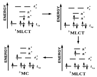
Figure 2: Orbital diagrams for the electronic GS and the most relevant excited states for pseudo-octahedral ruthenium(II) polypyridyl complexes.

$${}^{1}\mbox{GS}(t_{2g}^{6}\pi^{*0}e^{*0}_{g})\rightarrow{{}^{1}\mbox{MLCT}}(t_{2g}^{5}\pi^{*1}e^{*0}_{g})\,.$$ (1)

Ruthenium complex spin-orbit coupling then leads to rapid intersystem crossing to form the corresponding triplet ³MLCT$(t_{2g}^{5}\pi^{*1}e_{g}^{*0})$,

$${}^{1}\mbox{MLCT}(t_{2g}^{5}\pi^{*1}e^{*0}_{g})\rightarrow{{}^{3}\mbox{MLCT}}(t_{2g}^{5}\pi^{*1}e_{g}^{*0})\,.$$ (2)

This ³MLCT can phosphoresce back to the ¹GS or it can go over an excited-state transition state barrier to a triplet metal center state ³MC$(t_{2g}^{5}e_{g}^{*1}\pi^{*0})$,

$${}^{3}\mbox{MLCT}(t_{2g}^{5}\pi^{*1}e_{g}^{*0})\begin{array}[]{c}k_{a}\\ \rightarrow\\ \leftarrow\\ k_{b}\end{array}{{}^{3}\mbox{MC}}(t_{2g}^{5}e_{g}^{*1}\pi^{*0})\,.$$ (3)

Notice how the MC $e^{*}_{g}$ MO has now presumably become lower than the ligand-centered (LC) $\pi^{*}$ MO (Fig. 2). This is possible because of geometric relaxation as illustrated in the state diagram shown in Fig. 3. The resultant state can then go through a photochemical funnel with intersystem crossing to return to the groundstate,

$${}^{3}\mbox{MC}(t_{2g}^{5}e_{g}^{*1}\pi^{*0})\begin{array}[]{c}k_{c}\\ \rightarrow\end{array}{{}^{1}\mbox{GS}}(t_{2g}^{6}e_{g}^{*0}\pi^{*0})\,.$$ (4)

This is presumed to involve ligands coming partially or completely off and/or being replaced by solvent molecules. The rate constants $k_{a}$, $k_{b}$, and $k_{c}$ are the same as those defined in Ref. [21]. Figure 2 provides a summary in the form of orbitals and Figure 3 in the form of potential energy curves for different states.

Figure 3: The diagram shows the principle potential energy curves in our model. The abscissa corresponds to a reaction pathway involving partial removal of a ligand while the ordinate represents the state energy. The dashed lines indicate diabatic states whose avoided crossing leads to the energetic barrier on the adiabatic surface between the ³MLCT and ³MC minima. Figure from Ref. [3].

A key assumption is that the main luminescence quenching at room temperature is due to the barrier crossing [Eq. (3)] followed by a rapid return to the ground state [Eq. (4)]. For this reason, we will focus on this barrier in seeking a PDOS-LFT explanation for relative luminescence lifetimes, but let us admit in advance that our answer, though general and useful, is unlikely to be universal. For one thing, a mixture of different types of ligands or of different types of metal-ligand bonds, means that there is likely to be more than one path for luminescence quenching. Still other mechanisms might come in involving, say, unforeseen intermediate dark states. And, as we shall see in Sec. 3, the barrier crossing [Eq. (3)] is unlikely to be the only influence on the luminescence lifetime at room temperature. Nevertheless we shall be happy with a semi-quantitative PDOS-LFT-based theory of luminescence which works most of the time.

The rest of the paper is organized as follows: The next section discusses our choice of molecules, theoretical methods, and computational details. This is followed by a results section in which evidence is first given for the ability of DFT to give reasonably good geometries and of TD-DFT to give reasonably good absorption spectra. Secondly PDOS-LFT energy levels are discussed and shown to be useful for predicting photoproperties. And thirdly a model is presented which allows us to say something about luminescence lifetimes from PDOS-LFT energy levels. Section 4 concludes. PDOS and TD-DFT spectra are presented in a separate document as supporting information.

2 Data Base, Theoretical Method, and Computational Details

2.1 Data Base

Table 1: Numbering of the compounds investigated in this paper. With a few exceptions (listed but unnumbered compounds), these are the mononuclear complexes with 77 K experimental luminescence lifetimes taken in their order of occurance from Table 1 of Ref. [16]. An asterisk has been added if the original table also contained some information about room temperature lifetimes.

number	name
(1)*	[Ru(bpy)(CN)4]2-
(2)	[Ru(bpy)2Cl2]
(3)*	[Ru(bpy)2(CN)2]
(4)*	[Ru(bpy)2(en)]2+
(5)	[Ru(bpy)2(ox)]
(6)*	[Ru(bpy)3]2+
(7)*	[Ru(bpy)2(4-n-bpy)]2+
(8)*	[Ru(bpy)2(3,3’-dm-bpy)]2+
(9)*	[Ru(bpy)2(4,4’-dm-bpy)]2+
(10)*	[Ru(bpy)2(4,4’-dCl-bpy)]2+
(11)	[Ru(bpy)2(4,4’-dn-bpy)]2+
(12)*	[Ru(bpy)2(4,4’-dph-bpy)]2+
(13)*	[Ru(bpy)2(4,4’-DTB-bpy)]2+
(14)*	cis-[Ru(bpy)2(m-4,4’-bpy)2]4+
(15)*	[Ru(bpy)2(bpz)]2+
	[Ru(bpy)2(h-phen)]2+
(16)*	[Ru(bpy)2(phen)]2+
	[Ru(bpy)2(bpym)]2+
(17)	[Ru(bpy)2(4,7-dm-phen)2+
(18)*	[Ru(bpy)2(4,7-Ph2-phen)]2+
(19)*	[Ru(bpy)2(4,7-dhy-phen)]2+
(20)	[Ru(bpy)2(5,6-dm-phen)]2+
(21)	[Ru(bpy)2(DIAF)]2+
(22)*	[Ru(bpy)2(DIAFO)]2+
(23)*	[Ru(bpy)2(taphen)]2+
(24)	cis-[Ru(bpy)2(py)2]2+
(25)	trans-[Ru(bpy)2(py)2]2+
(26)	[Ru(bpy)2(pic)2]2+
(27)	[Ru(bpy)2(DPM)]2+
(28)	[Ru(bpy)2(DPE)]2+
(29)*	[Ru(bpy)2(PimH)]2+
(30)*	[Ru(bpy)2(PBzimH)]2+
(31)*	[Ru(bpy)2(biimH2)]2+
(32)*	[Ru(bpy)2(BiBzimH2)]2+
(33)	[Ru(bpy)2(NPP)]+
(34)	[Ru(bpy)2(piq)]2+
(35)	[Ru(bpy)2(hpiq)]2+

Table 2: Numbering of the compounds investigated in this paper. With a few exceptions (listed but unnumbered compounds), these are the mononuclear complexes with 77 K experimental luminescence lifetimes taken in their order of occurance from Table 1 of Ref. [16]. An asterisk has been added if the original table also contained some information about room temperature lifetimes.

number	name
(36)	[Ru(bpy)2(pq)]2+
(37)*	[Ru(bpy)2(DMCH)]2+
(38)	[Ru(bpy)2(OMCH)]2+
(39)*	[Ru(bpy)2(biq)]2+
(40)*	[Ru(bpy)2(i-biq)]2+
(41)*	[Ru(bpy)2(BL4)]2+
(42)*	[Ru(bpy)2(BL5)]2+
(43)*	[Ru(bpy)2(BL6)]2+
(44)*	[Ru(bpy)2(BL7)]2+
(45)*	[Ru(bpy)(3,3’-dm-bpy)2]2+
(46)*	[Ru(bpy)(4,4’-DTB-bpy)2]2+
(47)	[Ru(bpy)(h-phen)2]2+
(48)*	[Ru(bpy)(phen)2]2+
(49)	cis-[Ru(bpy)(phen)(py)2]2+
(50)	trans-[Ru(bpy)(phen)(py)2]2+
(51)	[Ru(bpy)(DIAFO)2]2+
(52)*	[Ru(bpy)(taphen)2]2+
(53)	[Ru(bpy)(py)2(en)]2+
(54)	[Ru(bpy)(py)3Cl]+
(55)	[Ru(bpy)(py)4]2+
(56)	[Ru(bpy)(py)2(PMA)]2+
(57)	[Ru(bpy)(py)2(2-AEP)]2+
(58)	[Ru(bpy)(PMA)2]2+
(59)	[Ru(bpy)(pq)2]2+
(60)*	[Ru(bpy)(DMCH)2]2+
(61)*	[Ru(bpy)(biq)2]2+
(62)*	[Ru(bpy)(i-biq)2]2+
(63)*	[Ru(bpy)(trpy)Cl]+
(64)*	[Ru(bpy)(trpy)(CN)]+
(65)*	[Ru(4-n-bpy)3]2+
(66)	[Ru(6-m-bpy)3]2+
(67)*	[Ru(3,3’-dm-bpy)3]2+
(68)	[Ru(3,3’-dm-bpy)2(phen)]2+
(69)	[Ru(3,3’-dm-bpy)(phen)2]2+
(70)*	[Ru(4,4’-dm-bpy)3]2+

Table 3: Numbering of the compounds investigated in this paper. With a few exceptions (listed but unnumbered compounds), these are the mononuclear complexes with 77 K experimental luminescence lifetimes taken in their order of occurance from Table 1 of Ref. [16]. An asterisk has been added if the original table also contained some information about room temperature lifetimes.

number	name
(71)*	[Ru(4,4’-dm-bpy)2(4,7-dhy-phen)]2+
(72)*	[Ru(4,4’-dCl-bpy)3]2+
(73)*	[Ru(4,4’-dph-bpy)3]2+
(74)*	[Ru(4,4’-DTB-bpy)3]2+
(75)	[Ru(6,6’-dm-bpy)3]2+
(76)	[Ru(h-phen)3]2+
(77)*	[Ru(phen)3]2+
(78)*	[Ru(phen)2(4,7-dhy-phen)]2+
(79)	[Ru(phen)2(pq)]2+
(80)	[Ru(phen)2(DMCH)]2+
(81)	[Ru(phen)2(biq)]2+
(82)	[Ru(phen)(pq)2]2+
(83)	[Ru(phen)(biq)2]2+
(84)	[Ru(2-m-phen)3]2+
(85)	[Ru(2,9-dm-phen)3]2+
(86)*	[Ru(4,7-Ph2-phen)3]2+
(87)*	[Ru(4,7-dhy-phen)(tm1-phen)2]2+
(88)	[Ru(DPA)3]-
(89)	[Ru(DPA)(DPAH)2]+
(90)	[Ru(DPAH)3]2+
(91)	[Ru(Azpy)3]2+
(92)	[Ru(NA)3]2+
(93)	[Ru(hpiq)3]2+
(94)	[Ru(pq)3]2+
(95)	[Ru(pq)2(biq)]2+
(96)	[Ru(pq)(biq)2]2+
(97)	[Ru(pynapy)3]2+
(98)*	[Ru(DMCH)2Cl2]
(99)*	[Ru(DMCH)2(CN)2]
(100)	[Ru(DMCH)3]2+
(101)	[Ru(dinapy)3]2+
(102)	[Ru(biq)2Cl2]
(103)*	[Ru(biq)2(CN)2]
(104)	[Ru(biq)3]2+
(105)	[Ru(i-biq)2Cl2]

Table 4: Numbering of the compounds investigated in this paper. With a few exceptions (listed but unnumbered compounds), these are the mononuclear complexes with 77 K experimental luminescence lifetimes taken in their order of occurance from Table 1 of Ref. [16]. An asterisk has been added if the original table also contained some information about room temperature lifetimes.

number	name
(106)*	[Ru(i-biq)2(CN)2]
(107)*	[Ru(i-biq)3]2+
(108)*	[Ru(trpy)2]2+
(109)	[Ru(tro)2]2+
(110)	[Ru(tsite)2]2+
(111)	[Ru(dqp)2]2+

Our theoretical calculations are based upon an old but unusually extensive list of the photoproperties of ruthenium complexes. In particular, our calculations are based upon the photoproperties of about 300 mononuclear ruthenium complexes reported in Table 1 of the 1988 review article of Juris, Balzini, Barigelletti, Capagna, Belser, and Von Zelewsky [16]. Of these, the 111 complexes shown in Tables 1, 2, 3, and 4 have luminescence data either at room temperature (RT) or at the boiling point of liquid nitrogen (77 K). For convenience we have numbered them in the same order as they appear in Table 1 of review article [16]. Note that this luminescence data was not necessarily measured in the same solvent for different compounds, or even for any given compound, and that the reported precision of the measurements vary. The ligand abbreviations are given in Appendix B. With a few exceptions (CN^-, Cl^-, ox, NPP, NA, bt, en), the ligands are pyridine and polypyridine N-type ligands, many of are found in common lists of the well-known spectrochemical series governing the ligand field splitting $\Delta$,

$$\Delta:\mbox{ Cl${}^{-}$ }<\mbox{ py }<\mbox{ en }<\mbox{ bpy }<\mbox{ phen }<\mbox{ CN${}^{-}$ }\,.$$ (5)

Calculations have been carried out on 98 of these 111 complexes, with 14 left untreated either because of lack of a good initial guess for the complex structure, convergence difficulties, or simple lack of time. Not every calculation is necessarily useful as some needed to be discarded for theoretical reasons (an unbound $e^{*}_{g}$ orbital) and not every property could be calculated for every compound. Furthermore we were not able to find comparison data for every property of every complex but we think that the extensiveness of our calculations and of the comparison with experiment for a broad range of complexes and properties should be highly useful.

2.2 Computational Methods and Details

The calculations reported in this paper are very similar to those reported in Ref. [3]. Version B.05 of the Gaussian 03 [22] quantum chemistry package was used in Ref. [3]. Here we use version D.01 of Gaussian 09 [23]. Density-functional theory (DFT) and time-dependent (TD-)DFT calculations were carried out using the same B3LYP functional. This is a three-parameter hybrid functional using Hartree-Fock (HF) exchange, the usual analytical form of the local density approximation (LDAx) for exchange [24], Becke’s 1988 generalized gradient approximation (GGA) exchange B88x [25], the Vosko-Wilk-Nusair parameterization of the LDA correlation (LDAc) [26], and Lee, Yang, and Parr’s GGA for correlation (LYP88c) [27],

$$E_{xc}^{\text{B3LYP}} = (1-a_{0})E_{x}^{\text{LDA}}$$

$$+ a_{0}E_{x}^{\text{HF}}+a_{x}E_{x}^{\text{B88x}}$$

$$+ a_{c}E_{c}^{\text{LYP88c}}+(1-a_{c})E_{c}^{\mbox{VWN80c}}\,,$$

where $a_{0}=0.20$, $a_{x}=0.72$, and $a_{c}=0.81$ are taken from Becke’s B3P functional [28].

These calculations require us to choose a Gaussian-type basis set. As in Ref. [3], we used the double-zeta quality LANL2DZ basis set for ruthenium along with the corresponding effective core potential (ECP) [29, 30]. All-electron 6-31G and 6-31G(d) basis sets [31, 32, 33, 34, 35, 36, 37] were used for all the elements in the first three periods of the periodic table. Note that Ref. [3] only used the smaller 6-31G basis set, while the present work is able to verify basis set convergence by also reporting results with the larger 6-31G(d) compounds. However, due to the very large number of calculations carried out and the size of the molecules, calculations with still larger basis sets were judged to fall outside of the scope of the present study. Unless otherwise mentioned, extensive use of program defaults was used for many of the computational parameters. Neither explicit nor dielectric cavity models were used in our calculations, so that all calculations reported in this article are technically for gas-phase molecules.

Table 5: List of 39 compounds with crystal structures. An asterisk indicates that the CCDC structure was modified.

Number	CCDC[38]	Citation
	reference code
(2)	AHEHIF	Ref. [39, 40]
(3)	LESLEB	Ref. [41]
(4)	SAXCIE	Ref. [42]
(5)	YAQJOP	Ref. [43]
(6)	BPYRUF	Ref. [44]
(7)	DIXVEL	Ref. [45]
(9)	JUQHEI	Ref. [46, 47]
(10)	BAQYEY	Ref. [48, 49]
(14)*	OBITIC01	Ref. [50, 51]
(16)	TIXFOV	Ref. [52]
(17)	XOFQEO	Ref. [53, 54]
(20)	IBAGAU	Ref. [55, 56]
(21)	COMVIJ	Ref. [57]
(22)	YAGJAR10	Ref. [58]
(24)	GEBHEA	Ref. [59]
(25)	QUBRIO	Ref. [60, 61]
(26)	MESWUC	Ref. [62, 63]
(31)	KEWQOT	Ref. [64, 65]
(32)	NUYKIC	Ref. [66, 67]
(33)	XOCXIW	Ref. [68]
(36)	HUWGEL	Ref. [69, 70]
(46)	QOMYEX	Ref. [71, 72]
(48)	JEMWAA	Ref. [73, 74]
(51)*	YAGJAR10	Ref. [58]
(62)*	PATLAX	Ref. [75]
(63)	WAKRUX	Ref. [76, 77]
(64)	NAMFOY	Ref. [78, 79]
(66)	FINREA	Ref. [80, 81]
(74)	NOFPII	Ref. [82, 83]
(75)	FINRIE	Ref. [84, 81]
(77)	ZIFCAU	Ref. [85, 86]
(81)	IFAXUI	Ref. [87, 88]
(83)	GEYZOB	Ref. [89, 90]
(84)	FINRAW	Ref. [91, 81]
(91)	MARVAD	Ref. [92, 93]
(94)	VAJLUO	Ref. [94, 95]
(107)	PATLAX	Ref. [75]
(108)	BENHUZ	Ref. [96, 97]
(109)	BOFGEJ	Ref. [98, 99]

The geometries of all the complexes were optimized and (local) minima were confirmed by the absence of imaginary vibrational frequencies. Whenever possible, the geometry optimizations began from X-ray crystal structural data obtained from the Cambridge Crystallographic Data Centre (CCDC) [100, 38]. This was the case for the compounds listed in Table 5. Start geometries indicated with an asterisk in Table 5 were constructed from the CCDC data of a related compound. Otherwise crystal coordinates were generated from the Gaussview program [101], taking into account specific symmetries and crystallographic volumes. The threshold for optimization was set to ultrafine with self consistent field (SCF) convergence being being set to very tight.

Time-dependent DFT [102, 103] gas-phase absorption spectra were calculated at the optimized ground-state geometries using the same functional and basis sets as for the ground-state calculation. In all cases, at least 100 singlet states were included in calculations of spectra. As in Ref. [3], a theoretical molar extinction spectrum is calculated via,

$$\epsilon(\omega)=\frac{\pi{N_{A}}e^{2}}{2\epsilon_{0}{m_{e}}c\,ln(10)}S(\omega)\,,$$ (7)

from the corresponding spectral function,

$$S(\omega)=\sum_{I}f_{I}\delta(\omega-\omega_{I})\,,$$ (8)

using an in-house python program Spectrum.py. The result is a theoretical spectrum with the same units and the same order of magnitude as the experimentally-measured absorption spectrum, thereby allowing easy comparison of theory and experiment, albeit at the expense of introducing a single empirical parameter which accounts for spectral broadening due to vibrational structure, solvent broadening (but not solvent shifts), and finite experimental resolution. This is the full width at half maximum (FWHM) which has been set to 40 nm throughout.

Density-of-states (DOS) and partial DOS (PDOS) were obtained using another in-house python program called Pdos.py previously described in the supplementary information associated with Ref. [3]. This allows us to identify the positions of ligand-field theory (LFT) like ruthenium $d$ states as well as ligand $\pi$ states after suitable broadening. At a practical level, using Pdos.py involves carrying out another single point calculation with the option (pop=full gfinput iop(6/7=3,3/33=1,3/36=-1), thereby causing Gaussian to output the number of basis functions Nbasis, the overlap matrix, the eigenvalues, and the MO coefficients. Pdos.py then takes this information from the Gaussian output files and calculates the (P)DOS. We used a FWHM of 0.25 eV with 40000 points for graphing.

3 Results

The results of our calculations are divided into three subsections. In the first subsection (Sec. 3.1), we validate the ability of DFT to be able to determine ground-state structures and the ability of TD-DFT to be able to simulate experimental absorption spectra. The second subsection (Sec. 3.2) extracts $t_{2g}$, $e^{*}_{g}$, and $\pi^{*}$ energies from PDOS-LFT and shows that these correlate with peaks in measured absorption spectra. The final subsection (Sec. 3.3) discusses the extent to which PDOS-LFT can be used to predict which compounds may have long luminescence lifetimes.

3.1 Structure and Properties

3.1.1 Geometries

We first test whether our DFT calculations are consistent with observed X-ray crystallography geometries by seeing how much typical bond lengths and bond angles change when the geometry is re-optimized in gas phase using the X-ray geometries as start geometries. Naturally we expect some expansion of the molecule as there are fewer constraints in the gas phase than in the solid phase but, nevertheless, we expect gas-phase and solid-state geometries to be correlated.

The need to judge correlation requires us to make a short review of linear regression as some of the concepts that we use are expected to be unfamiliar to even expert readers. Linear regression is just a least squares fit of $N$ $(x_{i},y_{i})$ data points to the familiar equation,

$$y=mx+b\,.$$ (9)

Minimizing the error

$${\cal E}=\sum_{i=1,N}\left(y_{i}-mx_{i}-b\right)^{2}\,,$$ (10)

gives the usual formulae for the slope and intercept,

$$m = \frac{\langle xy\rangle-\langle x\rangle\langle y\rangle}{\langle x^{2}\rangle-\langle x\rangle^{2}}$$

$$b = \frac{\langle y\rangle\langle xy\rangle-\langle x\rangle\langle xy\rangle}{\langle x^{2}\rangle-\langle x\rangle^{2}}\,,$$ (11)

where we have introduced the notation,

$$\langle f(x,y)\rangle=\frac{1}{N}\sum_{i=1,N}f(x_{i},y_{i})\,.$$ (12)

for the average of the $N$ $f(x_{i},y_{i})$ values. The goodness of fit is usually judged by the correlation coefficient defined as,

$$R^{2}=\frac{\left(\langle xy\rangle-\langle x\rangle\langle y\rangle\right)^{2}}{\left(\langle x^{2}\rangle-\langle x\rangle^{2}\right)\left(\langle y^{2}\rangle-\langle y\rangle^{2}\right)}\,,$$ (13)

which is close to unity for a good fit. Up to this point, everything corresponds to the standard formulae implemented in typical spreadsheet programs.

However, we need to go a little further because the correlation coefficient is not a good measure of the error in the sense that the correlation coefficient calculated over a small range of $x_{i}$ values may be very different from the correlation coefficient obtained when all the data is taken into consideration. That is why it is often better to calculate the standard error which is defined as the standard deviation of the $y_{i}$ values from those obtained from the fit. It may be calculated as,

$$\Delta y=\sqrt{\left(\frac{N}{N-2}\right)\left(\langle y^{2}\rangle-\langle y\rangle^{2}\right)\left(1-R^{2}\right)}\,,$$ (14)

which also shows the relation of the standard error to the correlation coefficient. Furthermore, following Ref. [104], it is often more interesting to invert the fit so that,

$$x=\frac{y}{m}-\frac{b}{m}\,.$$ (15)

The predictability,

$$\Delta x=\frac{\Delta y}{|m|}\,,$$ (16)

then represents the expected error in predicting the experimental results using our theoretical model. In reporting the results of our fits, we will give the slope $m$, the intercept $b$, the correlation coefficient $R$, and the predictability $\Delta x$.

In order to see how they are correlated, theoretical and experimental bond distances and angles were compared for 35 of the 39 complexes in Table 5. Complexes (14) and (62) are excluded because their start geometries were a modified version of the original X-ray crystal structures. Complexes (33) and (51) are excluded because we were unable to converge the gas-phase geometry optimizations.

(a)

(b)

Figure 4: (a) Correlation graph between calculated DFT bond lengths for the 6-31G ($\triangle$) and 6-31G(d) ($\circ$) and 184 measured X-ray crystallographic bond lengths. (b) Enlargement. The 45^∘ line indicates perfect agreement with experiment.

Figure 4 shows how calculated gas-phase bond lengths compare with X-ray crystal structure geometries. Only ligand-metal bond lengths have been considered. As expected the calculated gas-phase bond lengths are typically longer than those in the X-ray crystal structures. However Table 6 shows that the correlation is actually excellent with a predictability of 0.0251 Å for the 6-31G basis set and 0.0262 Å for the 6-31G(d) basis set. This may be compared with the typical error of 0.005 Å obtained for 20 organic molecules with the same functional and the 6-31G(d) basis set (p. 124 of Ref. [105]). Note, however, that the comparison made there is against gas phase data and that predicting the geometries of transition metal complexes is in general more challenging than predicting the geometries of purely organic molecules. It is interesting to note that geometries predicted using the 6-31G basis set are better correlated with experimental X-ray geometries obtained using the seemingly better 6-31G(d) basis set. This could be an indication that the 6-31G(d) basis set is less well balanced than is the 6-31G basis set. However the differences in the results obtained with the two basis sets are not really significant.

Table 6: Least squares fit parameters.

Basis Set	$m$	$b$	$R^{2}$	$\Delta x$
bond length/Å
6-31G	1.04387	-0.04195	0.90450	0.02505
6-31G(d)	1.02988	-0.00602	0.89674	0.02617
bond angles/degrees
6-31G	1.07230	-6.39743	0.93055	1.10263
6-31G(d)	1.07424	-6.79970	0.92682	1.13407
$\lambda$/nm
6-31G	0.78134	81.20545	0.47982	33.6319
6-31G(d)	0.77617	67.65579	0.40762	53.5672

(a)

(b)

Figure 5: (a) Correlation graph between calculated DFT bond angles for the 6-31G ($\triangle$) and 6-31G(d) ($\circ$) and 85 measured X-ray crystallographic bond angles. (b) Enlargement. The 45^∘ line indicates perfect agreement with experiment.

Figure 5 shows how calculated gas-phase bond angles compare with X-ray crystal structure geometries. Only ligand-metal-ligand angles near 90^∘ have been considered. The calculated bond angles tend to be smaller than the X-ray crystal structure bond angles. Table 6 shows that the correlation is actually excellent with a predictability of 1.103^∘ for the 6-31G basis set and 1.134^∘ for the 6-31G(d) basis set. This may be compared with the typical error quoted as being on the order of a few tenths of a degree obtained for 20 organic molecules with the same functional and the 6-31G(d) basis set (p. 124 of Ref. [105]). Of course, once again, this is not unexpected because the comparison is against gas phase data and that predicting the geometries of transition metal complexes is in general more challenging than predicting the geometries of purely organic molecules. It is also interesting to notice that, the 6-31G(d) basis set results correlated slightly less well with experiment than do the 6-31G basis set results, but the difference is not really significant.

3.1.2 Absorption Spectra

(a)

(b)

Figure 6: Comparison of calculated gas-phase absorption spectra (6-31G, red; 6-31G(d) blue) with an experimental spectrum: (a) complex (18), experimental spectrum in acetonitrile from Ref. [106]; (b) complex (24), experimental spectrum in water from Ref. [107].

We now wish to see if (TD-)DFT is able to give absorption spectra in reasonable agreement with experiment. Some example comparisons of spectra are given in Fig. 6. Many other TD-DFT spectra are given in the Supplementary Information. Note that no adjustable parameters have been used other than the FWHM (Sec. 2). Such spectra are expected to be accurate to about 0.2 eV, which is not extremely accurate but which is often adequate for qualitative assignments of spectral features. Typical complexes show two to four peaks, where some of the peaks are only visible as shoulders. Other spectra are given in the Supplementary Information. We have noticed that the lowest energy 6-31G(d) peak is often blue-shifted with respect to the corresponding 6-31G peak, with much less differences between the basis sets for higher-energy features in the TD-B3LYP spectra. The shift of the lower energy peak may indicate that the addition of $d$ functions is improving the description of the ground-state (i.e., lowering its energy) more than it is improving the description of the excited state. If so, this effect is less marked for higher excited states.

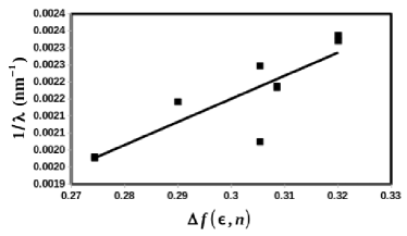
Figure 7: Inverse of the wavelength of the lowest energy absorption plotted against the orientational polarization for complex (3) and various solvents listed in Table 1 of Ref. [16], except for chloroform which did not fit the trend estabilished by the other solvents. Note that $\Delta f(\epsilon,n)=0.3054$ for acetonitrile.

In order to compare theory and experiment for several molecules, it is useful to focus on the lowest energy transition. Data for this has been collected from several references and is conveniently provided in Table 1 of Ref. [16] for several solvents. Since the lowest energy transition is expected to be of $t_{2g}\rightarrow\pi^{*}$ charge-transfer type, we can anticipate some solvent dependence, though it is often relatively small. We have tried to minimize solvent effects by estimating a best value in acetonitrile, a common solvent for polypyridinal ruthenium complexes. As discussed in Ref. [108], there are several ways to estimate solvent shifts in spectra and all involve approximations. The one we chose consists of seeking the best linear relationship between the inverse wavelength and the orientation polarizability,

$$\Delta f(\epsilon,n)=\frac{\epsilon-1}{2\epsilon+1}-\frac{n^{2}-1}{2n^{2}+1}\,,$$ (17)

which comes out of Onsager’s reaction field theory. Here $\epsilon$ is the solvent dielectric constant and $n$ is the solvent refractive index. Note that this is only valid for a given transition weakly interacting with a dielectric medium. An example plot is shown in Fig. 7 for complex (3) where the solvent shift is particularly marked and there are two experimental values for the absorption in acetonitrile. The value from the linear plot for this compound and best estimates in acetonitrile where they could be extracted are shown in Table 7.

Table 7: Best estimates of the lowest energy absorption maximum in acetonitrile based upon data from Table 1 of Ref. [16].

number	wavelength	number	wavelength
	(nm)		(nm)
(1)	431.2	(53)	476.0
(2)	524.0	(56)	465.0
(3)	457.2	(57)	455.0
(6)	451.5	(58)	478.0
(7)	493.0	(59)	479.1
(8)	448.0	(60)	559.0
(9)	445.0	(61)	547.0
(10)	448.0	(62)	450.0
(11)	514.0	(63)	506.0
(12)	458.0	(64)	487.3
(13)	450.0	(65)	480.0
(14)	450.0	(66)	448.0
(15)	472.7	(67)	456.0
(22)	440.0	(70)	456.0
(23)	440.0	(72)	462.0
(24)	450.0	(73)	474.0
(25)	474.0	(74)	456.0
(29)	460.0	(76)	453.0
(30)	458.0	(77)	467.4
(31)	473.0	(79)	483.0
(32)	463.0	(80)	522.0
(34)	483.0	(81)	522.0
(35)	480.0	(90)	375.0
(36)	478.0	(92)	505.0
(37)	528.0	(93)	494.0
(38)	562.0	(94)	483.5
(39)	526.0	(97)	526.0
(40)	540.0	(99)	605.1
(45)	453.0	(100)	540.0
(46)	454.0	(101)	585.0
(47)	450.0	(103)	605.1
(48)	442.0	(104)	524.0
(49)	448.0	(105)	436.0
(50)	476.0	(106)	414.8
(51)	446.0	(107)	392.0
(52)	438.0	(108)	473.1

Figure 8: Correlation graph between calculated lowest energy absorption wavelengths for the 6-31G ($+$) and 6-31G(d) ($\times$) and 59 best estimates for the best estimate of the experimental lowest energy absorption wavelengths in acetonitrile, all in nm. The 45^∘ line indicates perfect agreement with experiment.

Figure 8 shows how our TD-DFT spectra compare with experimental spectra for the placement of the lowest energy absorption maximum. The calculated predictability shown in Table 6 corresponds to 0.17 eV for the 6-31G basis set and to 0.27 eV for the 6-31G(d) basis set at 500 nm. This is the sort of accuracy we normally expect from TD-DFT in the absence of any particular problems such as, say, strong density relaxation upon excitation. We conclude that our DFT model is a reasonably good descriptor of the experimental situation.

3.2 PDOS-LFT

We now come to the heart of this paper, namely the partial density-of-states (PDOS) technique for extracting ligand field theory (LFT) like information from DFT calculations. This is needed by chemists as it is their traditional tool for thinking about and discussing spectra (e.g., Fig. 6) and other photoprocesses in transition metal complexes. It is also nontrivial because the usual pseudo-octahedral orbitals $t_{2g}$ and $e^{*}_{g}$ do not emerge automatically from DFT calculations. This statement is less true of the nonbonding $t_{2g}$ which can often be identified by direct visualization of DFT molecular orbitals, but it is very true of the antibonding $e^{*}_{g}$ orbitals which (because they are antibonding) mix heavily with ligand orbitals, making it impossible to identify individual $e^{*}_{g}$ orbitals among the DFT molecular orbitals in the absence of special tools. The tool we have used here is the very simple one used in Ref. [3], namely a PDOS analysis based upon Mulliken charges. Other (P)DOS graphs may be found in the Supplementary Information.

(a)

(b)

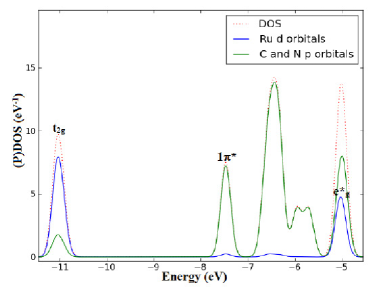
Figure 9: B3LYP/6-31G (P)DOS calculated for (a) complex (18) and (b) complex (24). Note that the corresponding highest-occupied molecular orbital energies are -10.43 eV for complex (18) and -10.95 for complex (24).

The concept of the density-of-states (DOS) is borrowed from solid-state physics. The idea is to replace the orbital energy levels, which have become too dense for convenient interpretation, with a gaussian-broadened stick spectrum,

$$\mbox{DOS}(\epsilon)=\sum_{i}g(\epsilon-\epsilon_{i})\,,$$ (18)

where the gaussian,

$$g(\epsilon)=\sqrt{\frac{\alpha}{\pi}}e^{-\alpha x^{2}}\,,$$ (19)

is normalized to unity. The parameter $\alpha$ is fixed by the FWHM according to the relation,

$$\mbox{FWHM}=2\sqrt{\frac{\ln 2}{\alpha}}\,.$$ (20)

We loose the concept of individual orbital energy levels when using the DOS. Nevertheless an isolated DOS peak of unit area corresponds to a single underlying orbital energy level, a DOS peak integrating to an area of two corresponds to two closely spaced underlying orbital energy levels, etc. Figure 9 provides an example of the DOS of two complexes. Note that each peak represents one to several underlying molecular orbital levels.

The partial density-of-states (PDOS) goes a step further by introducing an atomic orbital decomposition of the DOS. Thus the PDOS for the $\mu$th atomic orbital is,

$$\mbox{PDOS}_{\mu}(\epsilon)=\sum_{i}q_{\mu,i}g(\epsilon-\epsilon_{i})\,.$$ (21)

Here the quantity $q_{\mu,i}$ is the Mulliken atomic charge of atomic orbital $\mu$ in molecular orbital $i$. We obtain the ruthenium $d$ PDOS by summing PDOS_μ over all $d$-type atomic orbitals on ruthenium. Similarly we obtain the $\pi$ PDOS by summing PDOS_μ over all the $p$-type atomic orbitals on the heavy atoms (e.g., on C, N, and O) on the ligands. As seen in Fig. 9, the approximate energies of the $t_{2g}$ and $e^{*}_{g}$ orbitals on the ruthenium clearly emerge for complex (24) with the expected peak height ratio of 3:2. We also see a loss of $t_{2g}$ degeneracy for complex (18) due to breaking of perfect octahedral symmetry in this complex as well as some small seemingly random $d$-orbital density contributing to molecular orbitals at other energies.

(a)

(b)

Figure 10: B3LYP (P)DOS calculated for complex (18): (a) 6-31G basis and (b) 6-31G(d) basis.

It should be noted that the PDOS analysis, while highly useful, also contains a degree of arbitrariness. In the first place, the precise picture will vary as the FWHM is varied. This is why it is best to use a fixed value of the FWHM as we do in this paper. Also, the PDOS shares the basis-dependence of the Mulliken analysis. This is illustrated in Fig. 10 where the $e^{*}_{g}$ peak shifts slightly relative to the $\pi^{*}$ peaks when going from the 6-31G to the 6-31G(d) basis set. Many other examples allowing the comparison of the PDOS calculated with the two different basis sets for a wide variety of complexes may be found in the Supplementary Information and provide further evidence for slight basis-set dependent shifts in the PDOS. However an important exception is in the case of unbound (i.e., positive energy) orbitals where a finite basis set is trying to describe a continuum. These cases are marked with an asterisk (*) in the Supplementary Information and can show very great differences between the position and character of the $t_{2g}$ and $e^{*}_{g}$ PDOS peaks in going from the 6-31G to the 6-31G(d) basis sets, such as is the case for complex (7)* where there is a simple $t_{2g}$ peak in the PDOS calculated with the 6-31G basis set and a triple $t_{2g}$ peak in the PDOS calculated with the 6-31G(d) basis set.

Figure 11: Correlation plot between $\Delta_{\mbox{PDOS-LFT}}$ calculated in cm^-1 with the 6-31G and 6-31G(d) basis sets for 55 complexes. The diagonal line indicates where points should lie in the event of hypothetical perfect agreement between the two sets of results. A least squares fit to the calculated points gives the equation $\Delta_{\mbox{PDOS-LFT}}$(6-31G(d)) = 0.940 $\Delta_{\mbox{PDOS-LFT}}$(6-31G) + 1740. cm^-1. Complexes whose data points are marked: (6) [Ru(bpy)₃]²⁺, (42) [Ru(bpy)₂(BL5)]²⁺, (107) [Ru(i-biq)₂(BL5)]²⁺, (93) [Ru(hpiq)₃]²⁺, (75) [Ru(6,6’-dm-bpy)₃]²⁺, (85) [Ru(2,9-dm-phen)₃]²⁺, (96) [Ru(pq)(biq)₂]²⁺, and (104) [Ru(biq)₃]²⁺.

Table 8: $\Delta_{\text{PDOS-LFT}}$ (cm^-1) for complexes with simple $t_{2g}$ and $e^{*}_{g}$ peaks.

number	6-31G	6-31G(d)
(6)	49 300.	48 200.
(8)	48 800.	48 100.
(9)	48 900.	48 000.
(11)	49 300.	47 800.
(13)	49 100.	47 900.
(14)	47 800.	46 900.
(15)	49 500.	48 300.
(16)	48 800.	47 800.
(17)	48 300.	47 400.
(19)	47 800.	46 500.
(20)	48 800.	47 400.
(23)	48 400.	47 400.
(24)	48 400.	47 300.
(25)	48 400.	47 100.
(26)	48 300.	47 200.
(27)	48 000.	46 800.
(28)	47 700.	46 700.
(29)	48 700.	47 500.
(30)	48 500.	47 500.
(31)	48 500.	47 000.
(32)	48 000.	46 700.
(34)	49 000.	47 900.
(40)	48 700.	47 400.
(41)	48 900.	47 700.
(42)	48 800.	48 000.
(46)	48 900.	47 700.
(47)	48 800.	47 600.
(48)	48 700.	47 200.
(50)	48 300.	47 100.

Table 9: $\Delta_{\text{PDOS-LFT}}$ (cm^-1) for complexes with simple $t_{2g}$ and $e^{*}_{g}$ peaks.

number	6-31G	6-31G(d)
(52)	48 100.	46 800.
(53)	47 400.	46 700.
(55)	47 100.	45 700.
(56)	47 700.	46 600.
(57)	47 300.	46 300.
(58)	47 600.	46 400.
(70)	48 300.	47 500.
(71)	47 800.	46 600.
(75)	45 400.	44 700.
(76)	48 400.	47 600.
(77)	48 300.	47 300.
(78)	47 800.	46 600.
(85)	43 800.	43 400.
(87)	47 700.	46 300.
(90)	47 400.	45 700.
(93)	47 500.	46 600.
(94)	46 100.	44 700.
(96)	43 600.	42 500.
(97)	48 500.	47 100.
(104)	43 000.	42 200.
(107)	48 000.	47 400.

We thus have a ligand-field theory (LFT) like PDOS-LFT picture. However it is not LFT as the PDOS-LFT splitting $\Delta_{\text{PDOS-LFT}}$ calculated as the energy difference between the $e^{*}_{g}$ and $t_{2g}$ PDOS peaks is not the same as the $\Delta_{\text{LFT}}$ expected from LFT. We can see this by comparing numbers for the much studied complex (6). According to our calculations, $\Delta_{\text{PDOS-LFT}}=$49 300 cm^-1 calculated with the 6-31G basis set and 48 200 cm^-1 calculated with the 6-31G(d) basis set. This can be compared with the value $\Delta_{\text{PDOS-LFT}}=$48 000 cm^-1 and with $\Delta_{\text{LFT}}=$28 600 cm^-1 reported previously [3]. Clearly $\Delta_{\text{PDOS-LFT}}$ is much larger than $\Delta_{\text{LFT}}$ so that PDOS-LFT is different from the usual LFT.

Tables 8 and 9 show the values of $\Delta_{\text{PDOS-LFT}}$ for complexes sufficiently close to octahedral symmetry to show simple $t_{2g}$ and $e^{*}_{g}$ PDOS peaks, excluding complexes where the $e^{*}_{g}$ peak is unbound. Figure 11 provides a graphical comparison of how $\Delta_{\text{PDOS-LFT}}$ changes in going from the 6-31G to the 6-31G(d) basis set. The correlation is linear up to some residual scatter which can be explained by the precision of the graphical measurement of the distance between peaks. In general, the $\Delta_{\text{PDOS-LFT}}$ splitting closes a bit when the larger basis set is used compared to the smaller basis set. Although $\Delta_{\text{PDOS-LFT}}\neq\Delta_{\text{LFT}}$, we do expect them to have the same trends and so to be able to establish spectrochemical series. Thus from Fig. 11 we may, for example, deduce the following relationship for ligand field strength:

$$\Delta : > > > >$$ bpy i-biq hpiq DPAH pq

$$> \mbox{6,6'-dm-bpy $>$ 2,9-dm-phen $>$ biq}\,.$$

Ligand abbreviations are defined in Appendix B.

Figure 12: Correlation plot between $t_{2g}\rightarrow\pi^{*}$ PDOS orbital energy differences calculated using the 6-31G basis set and TD-B3LYP(6-31G) absorption spectra peaks. A least squares fit to the 161 data points gives the line indicated on the graph whose equation is $\lambda(\omega_{S})=1.19\lambda(\epsilon_{\pi^{*}}-\epsilon_{t_{2g}})-+\mbox{7.63 nm}$.

Since the usual LFT splitting $\Delta_{\text{LFT}}$ is extracted from absorption spectra [14], it is interesting to see to what extent energy differences between PDOS-LFT peaks correlate with the position of TD-DFT absorption spectra peaks. Often times, TD-DFT results may be analyzed within the two-orbital two-electron model (TOTEM) (See, e.g., the review Ref. [103]). Let us consider a simpler hybrid functional,

$$E_{xc}^{\text{Hybrid}}=(1-a_{0})E_{x}^{\text{GGA}}+a_{0}E_{x}^{\text{HF}}+E_{c}^{\text{GGA}}\,,$$ (23)

than the B3LYP functional [Eq. (LABEL:eq:details.1.5)] as it already captures all the essential features which are of interest to us here. In the Tamm-Dancoff approximation (See, e.g., the review Ref. [103]), the TOTEM model gives the following formulae for the singlet $\omega_{S}$ and triplet $\omega_{T}$ excitation energies:

$$\omega_{S}^{\text{Hybrid}} = \epsilon_{a}-\epsilon_{i}+2(ia|f_{H}|ai)$$

$$- a_{0}(ii|f_{H}|aa)+(1-a_{0})(ia|f_{x}^{\alpha,\alpha}|ai)$$

$$+ a_{c}(ia|f_{c}^{\alpha,\alpha}+f_{c}^{\alpha,\beta}|ai)$$

$$\omega_{T}^{\text{Hybrid}} = \epsilon_{a}-\epsilon_{i}$$ (24)

$$+ (1-a_{0})(ia|f_{x}^{\alpha,\alpha}|ai)$$

$$+ a_{c}(ia|f_{c}^{\alpha,\alpha}-f_{c}^{\alpha,\beta}|ai)\,,$$

where we follow the notation of Ref. [103]. If the two-electron integrals are (or their sum is) sufficiently small, then we may expect that excitation energies may be approximated, albeit rather roughly, as orbital energy differences:

$$\omega\approx\epsilon_{a}-\epsilon_{i}\,.$$ (25)

This was checked by taking the same complexes treated in Fig. 11 and comparing the wavelength corresponding to the $\epsilon_{t_{2g}}\rightarrow\epsilon_{\pi^{*}}$ transitions with the wavelength of the corresponding peaks in the TD-B3LYP absorption spectra in Fig. 12. A least squares fit indicates quite a good correlation in the sense that the slope is only slightly greater than unity and the intercept is small. However there is a large scatter of the data points around the fit line which may be due to neglect of two-electron integrals but may equally well be due to difficulty assigning the precise positions of PDOS peaks and of peaks (and particularly of shoulders) in the TD-B3LYP spectra. Nevertheless we find the figure to be quite encouraging in that the figure suggests that a PDOS-LFT orbital model may provide useful insight into the behavior of excited states.

3.3 Luminescence Lifetimes

Figure 13: Correlation between luminescence lifetimes at room temperature (RT) and at liquid nitrogen temperature (77K).

Table 10: Compounds with both room temperature (RT) and liquid nitrogen temperature (77K) data from Table 1 of Ref. [16]. An asterisk has been added if the PDOS $e_{g}^{*}$ orbital is unbound. Luminescence times are averages over different measurements in different solvents. See text for the definition of $\Delta E_{\text{ave}}$.

number	$\tau$(77K)	$\tau$(RT)	$\Delta E_{\text{ave}}$
	$\mu$s	$\mu$s	cm-1
(1)*	3.7	0.043	321.
(3)*	3.7	0.30	181.
(4)	0.84	0.070	179.
(6)	5.23	0.845	132.
(7)*	3.1	0.78	100.
(8)	5.25	0.533	165.
(9)	5.2	0.48	172.
(12)	5.6	1.92	77.
(13)	4.6	1.17	99.
(14)	7.59	0.454	203.
(15)	3.4	0.378	158.
(16)	6.6	0.497	186.
(18)	9.4	1.591	128.
(19)	3.9	0.628	132.
(21)	5.9	0.00007	818.
(22)	5.1	0.137	261.
(23)	1.8	0.05	259.
(29)	4.450	0.192	227.
(30)	4.240	0.340	182.
(31)	3.25	0.121	237.
(32)	3.000	0.115	235.
(37)	1.5	0.38	99.
(39)	1.65	0.27	131.
(40)	4.7	1.1	105.

Table 11: Compounds with both room temperature (RT) and liquid nitrogen temperature (77K) data from Table 1 of Ref. [16]. An asterisk has been added if the PDOS $e_{g}^{*}$ orbital is unbound. Luminescence times are averages over different measurements in different solvents. See text for the definition of $\Delta E_{\text{ave}}$.

number	$\tau$(77K)	$\tau$(RT)	$\Delta E_{\text{ave}}$
	$\mu$s	$\mu$s	cm-1
(41)	4.560	0.356	184.
(42)	4.090	0.390	170.
(43)	4.020	0.389	169.
(44)	4.070	0.360	175.
(46)	4.8	1.07	108.
(48)	12.45	0.784	200.
(52)	2.0	0.13	197.
(60)	1.9	0.39	114.
(61)	1.95	0.20	164.
(64)*	5.0	0.001	615.
(67)*	6.4	0.21	632.
(70)	4.6	0.525	157.
(71)	10.50	0.475	223.
(73)	4.79	1.31	94.
(74)	5.3	1.15	110.
(77)	9.93	0.673	194.
(78)	3.0	1.675	42.
(86)	9.58	4.796	50.
(87)	11.0	1.750	132.
(99)*	1.17	0.167	115.
(103)*	0.88	0.147	129.
(106)*	177.	0.237	477.
(107)	96.0	0.1475	467.
(108)	10.7	0.0037	575.

Since gas-phase B3LYP geometries are a good indicator of ruthenium complex crystal geometries, gas-phase TD-B3LYP geometries are a reasonable indicator of ruthenium complex absorption spectra in solution, and PDOS-LFT energies provide a first approximation to absorption spectra energies, then we may also hope to be able to say something about ruthenium complex luminescence lifetimes on the basis of PDOS-LFT information. Indeed this was the reasoning given in the seminal paper [3] where PDOS-LFT luminescence indices were proposed upon the basis of the idea that the room temperature (RT) luminescence lifetime should increase with the height of the ³MLCT $\rightarrow$ ³MC barrier shown in Fig. 3. This barrier-height dependence would also imply a strong temperature dependence which is indeed seen in the 48 liquid nitrogen (77 K) and room temperature (RT) values in Tables 10 and 11 and the 46 points in Fig. 13.

In order to see where PDOS-LFT-derived luminescence indices may be able to say something about luminescence lifetimes, we need first to understand the various contributions to luminescence lifetimes. Luminescence lifetime experiments measure the decay rate of the intensity of light luminescing at a particular wavelength as a function of time. This gives a temperature ($T$) dependent decay constant $k(T)$ which is related to the decay lifetime $\tau(T)$ by,

$$k(T)=\frac{1}{\tau(T)}\,.$$ (26)

The luminescence lifetime determined from the decay rate of measured intensity is a measure of the rate of disappearance of the luminescent species — in this case, the phosphorescent ³MLCT state. In addition to phosphorescence, other physical phenomena are also included in the decay lifetime $\tau(T)$ which generally depend upon the temperature $T$. The decay rate constant may be separated,

$$k(T)=k_{0}+k_{b}^{nr}(T)\,,$$ (27)

into a temperature-independent part,

$$k_{0}=k^{r}+k_{a}^{nr}\,,$$ (28)

where the superscript “r” refers to “radiative” and the superscript “nr” refers to “nonradiative” [109]. The temperature-independent part describes processes which continue to be operational even at very low temperatures. ($k_{0}$ is assumed to be equal to $k(T)$ at $T$ = 84 K in Ref. [110].) The temperature-dependent part may be further separated as [16],

$$k_{b}^{nr}(T)=k_{\text{melt}}(T)+k_{\text{equlib}}(T)+k_{\text{barrier}}(T)\,,$$ (29)

where,

$$k_{\text{melt}}(T)=\frac{B}{1+\exp\left[C\left(\frac{1}{T}-\frac{1}{T_{B}}\right)\right]}$$ (30)

describes the melting of the solid matrix of the solution at low temperature, where $k_{\text{melt}}(T)$ = constant $B$ for T$\rightarrow\infty$ and $k_{\text{melt}}(T)=0$ for T$\rightarrow$0. $T_{B}$ is the temperature at which $k_{\text{melt}}(T)$=B/2 and C is a temperature related to the viscosity effect;

$$k_{\text{equlib}}(T)=A_{1}e^{-\Delta E_{1}/RT}\,,$$ (31)

describes thermal equilibrium with higher energy states of the same electronic nature (e.g., states with the same symmetry in an octahedral complex according to LFT but which are split with ligands giving only pseudo-octahedral symmetry), and

$$k_{\text{barrier}}(T)=A_{2}e^{-\Delta E_{2}/RT}\,,$$ (32)

is an Arrhenius term describing crossing of the ³MLCT $\rightarrow$ ³MC barrier prior to subsequent de-activation to ¹GS. As pointed out in Ref. [21], $\Delta E_{2}$ is only the ³MLCT $\rightarrow$ ³MC activation energy barrier when $k_{c}>>k_{b}$ [see Eqs. (3) and (4)], but the situation becomes more complicated if (for example) $k_{b}>>k_{c}$. Putting it altogether results in,

$$k = k_{0}+k_{\text{melt}}(T)+k_{\text{equlib}}(T)+k_{\text{barrier}}(T)$$ (33)

$$= k_{0}+\frac{B}{1+\exp\left[C\left(\frac{1}{T}-\frac{1}{T_{B}}\right)\right]}$$

$$+ A_{1}e^{-\Delta E_{1}/RT}+A_{2}e^{-\Delta E_{2}/RT}\,.$$

The barrier term is commonly believed to dominate over the other terms at high-enough temperatures. If so, then we may hope to be able to relate $\Delta E_{2}$ to the features of the PDOS-LFT theory.

Table 12: Parameters describing the temperature dependence of the luminescence decay rate of [Ru(bpy)₃]²⁺ in propionitrile/buylronitile (4:5 v/v) from p. 108 of Ref. [16], except: $C$ and $T_{B}$ were determined by variation within the recommended range until we obtained results similar to those in Fig. 6 of Ref. [110]. $A_{\text{ave}}$ and $\Delta E_{\text{ave}}$ are calculated as explained in the text.

parameter	value
$k_{0}$	2 $\times$ 105 s-1
$B$	2.1 $\times$ 105 s-1
$C$	1900
$T_{B}$	125 K
$A_{1}$	5.6 $\times$ 105 s-1
$\Delta E_{1}$	90 cm-1
$A_{2}$	1.3 $\times$ 1014 s-1
$\Delta E_{2}$	3960 cm-1
$A_{ave}$	2.707 $\times$ 106 s-1
$\Delta E_{ave}$	159.98 cm-1

Figure 14: Plot of $\ln(k)$ versus $1/T$ for luminescence decay rates for [Ru(bpy)₃]²⁺ in propionitile/butyronitrile (4:5 v/v).

But how high a temperature is high-enough to make this hope reasonable? We can get some idea of the answer to this question by examination of the relative importance of the different terms in Eq. (29) for [Ru(bpy)₃]²⁺ in propionitrile/butyronitrile (4:5 v/v) using the parameters given in Table 12. Data is often plotted as $\ln(k)$ versus $1/T$ as shown in Fig. 14. A look at the different contributions on the excited state lifetimes is also shown on the same plot. It looks very different on different scales as different physical effects come into play in different temperature regimes. Only $k_{0}$ is important below about 30 K. From about 30 K to 100 K, $k_{\text{equilib}}$ becomes important. The melting term $k_{\text{melt}}$ switches on from about 100 K to about 250 K. After 250 K, $k_{\text{barrier}}$ rapidly begins to dominate. Unfortunately $k_{\text{barrier}}$ is not the single overwhelmingly dominant term at RT (298 K).

This means that it is very difficult to extract an accurate value of the triplet barrier energy $\Delta E_{2}$ from only the luminescence decay constants at 77 K and at RT. We have tried various ways to do so, but all of them suffer from some sort of numerical instability resulting from trying to get a relatively small number from taking the difference of two large numbers. Improved computational precision would not solve this problem because the accuracy of the two large numbers is limited by experimental precision. We therefore choose a different route and simply assume that RT is a high-enough temperature to neglect all but the barrier term. Figure 14 shows that this is only a very rough approximation at best. However we have little alternative but to make this approximation given the nature of the primary readily available data. That is, the best that can be done if the only data available is the luminescence decay constants at 77 K and at RT, is to fit to the very simple equation,

$$k(T)=A_{\text{ave}}e^{-\Delta E_{\text{ave}}/RT}\,.$$ (34)

This may also be regarded as an alternative (overly simplistic) model. If we can use this model to explain how $\Delta E_{\text{ave}}$ may be estimated from PDOS-LFT, then we will nevertheless have access to information about the interrelationship of luminescence lifetimes at 77 K and at RT. With this caveat, we will confine subsequent discussion to luminescence indices for predicting $\Delta E_{\text{ave}}$.

Figure 15: Correlation between $\Delta E$ and $E_{\text{ave}}$.

Let us now turn to the challenge posed in Ref. [3], namely that of coming up with MO-based indices (or, more exactly, PDOS-LFT-based indices) for predicting luminescence lifetimes. The argument was made that the $\Delta E_{\text{ave}}$ should be largest when the ³MC-³MLCT state energy difference is smallest. In LFT-PDOS terms, this corresponds to $\Delta E_{\text{ave}}$ being smallest when the MO energy difference,

$$\Delta E=\epsilon_{e_{g}^{*}}-\epsilon_{\pi^{*}}\,,$$ (35)

is smallest. We can check this using the PDOS corresponding to the complexes listed in Tables 10 and 11. A few complexes have to be eliminated when the known underbinding of DFT has led to unbound $e^{*}_{g}$ orbitals. Nevertheless, this still leaves 36 data points. The correlation between $\Delta E$ and $E_{\text{ave}}$ is shown in Fig. 15. The correlation is surprisingly bad.

Figure 16: Correlation between $1/\Delta E$ and $E_{\text{ave}}$. The dashed line is only a guide to the eye.

We are thus led to think more deeply about the avoided crossing of two states with diabatic energies $E_{1}$ and $E_{2}$ and coupling matrix element $W$. The adiabatic energies may be found by diagonalizing the two-state hamiltonian matrix,

$${\bf H}=\left[\begin{array}[]{cc}E_{1}&W\\ W&E_{2}\end{array}\right]\,.$$ (36)

The exact and perturbative solutions are,

$$E_{+} = \bar{E}+\frac{1}{2}\sqrt{\left(\Delta E\right)^{2}+4W^{2}}$$

$$\approx E_{2}-\frac{W^{2}}{\Delta E}$$

$$E_{-} = \bar{E}-\frac{1}{2}\sqrt{\left(\Delta E\right)^{2}+4W^{2}}$$ (37)

$$\approx E_{1}+\frac{W^{2}}{\Delta E}\,,$$

where

$$\bar{E}=\frac{E_{1}+E_{2}}{2}\,.$$ (38)

is the average of the diagonal elements. Following ideas very similar to those found in frontier MO theory (FMOT) [111, 112], we will adapt the pertubative formulae evaluated at the ground state geometry,

$$E_{-}-E_{1}\approx\frac{W^{2}}{\Delta E}\,.$$ (39)

as the estimate of the triplet state energy barrier. More exactly, the slope of the potential energy curve for the excited state at the ground-state equilibrium geometry provides a rough indication of trends in the height of the excited-state energy barrier. Although we are not actually doing FMOT, but rather presenting something which we suppose to be novel, it should be born in mind that our theory resembles FMOT and so is subject to criticism similar to that which Dewar so reasonably leveled at FMOT [113]. Nevertheless FMOT continues to be used and indeed was honored by the 1981 Nobel Prize in Chemistry because, occasional failures set aside, FMOT frequently provides a simple explanation of chemical reactivity. Likewise we seek a simple explanation of luminesence lifetimes but expect there to be occasional exceptions. Equation 39 suggests that $E_{\text{ave}}$ should correlate better with $1/\Delta E$ than with $\Delta E$. This hypothesis is tested in Fig. 16. Figure 16 does indeed seem more linear than does Fig. 15, but the line in Fig. 16 seems to take the form of an upperbound to a scatter of $E_{\text{ave}}$ values.

Figure 17: Correlation between $\bar{E}^{2}/\Delta E$ and $E_{\text{ave}}$. The dashed line is only a guide to the eye.

A clue as to how to further improve our theory is to notice that while $E_{\text{ave}}$ has units of energy, $1/\Delta E$ has units of inverse energy. This should be corrected by the quantity $W$ which also has units of energy, but which is not obviously related to the PDOS-LFT picture from which we seek to extract clues about luminescence lifetimes. Again, we take our lead from Roald Hoffmann (one of the fathers of FMOT), and estimate $W$ by the Wolfberg-Helmholtz-like formula [114],

$$W=S\bar{E}\,,$$ (40)

where $\bar{E}$ was defined in Eq. (38) and $S$ is some sort of overlap matrix element. Let us assume that $S\approx$ constant, and so compare $E_{\text{ave}}$ against $\bar{E}^{2}/\Delta E$ which both have the energy units. The result is shown in Fig. 17. Except for a few complexes [(14), (21), (107), (108), and possibly ((78)], the result is finally a reasonably good linear correlation. Indeed a least squares fit [$E_{\text{ave}}=(\mbox{9.348 cm${}^{-1}$/eV})(\bar{E}^{2}/\Delta E)+\mbox{50.764 cm${}^{-1}$}$] indicates that the line passes pretty nearly through the origin as might be expected from our simple FMOT-like theory.

In principle we might be able to do better by being able to provide some suitable estimate of the overlap $S$. One suggestion was given in Ref. [3] which involved the percentage of $d$ contribution to the $\pi^{*}$ peak times the percentage of $\pi$ contribution to the $t_{2g}$ peak. We have tried this and several other similar ideas as a way to construct an estimate of $S$ and have found no way to improve upon $\bar{E}^{2}/\Delta E$ as the best estimator of $E_{\text{ave}}$. We therefore conclude that this is the best we are going to obtain. The outliers in Fig. 17 (i.e., those far from the line correlating $E_{\text{ave}}$ with $\bar{E}^{2}/\Delta E$ might easily be accounted for by such things as the roughness of the estimates of luminescence lifetimes which, on the one hand, are not always reported very accurately and which, on the other hand, have been averaged over different values in different solvents. It is also possible that not all ruthenium complexes have the same type of decay mechanism — and varying the ligands is an excellent way to increase the number of ways a ligand can come off and go on again, leading us back to the ground state. Indeed, as explained above, we do not even expect our FMOT-like approach to work 100% of the time and so are happy that it works as well as it seems to work.

4 Conclusion

We have shown that gas-phase DFT and TD-DFT calculations give results that correlate well with crystal geometries and with solution absorption spectra of ruthenium complex spectra. This is not really a surprise. It has been noticed before and has even been treated in review articles focusing on the spectra of transition metal complexes [115, 116, 117]. However quantifying this relationship for a very large group of ruthenium(II) polypyridine complexes is already useful.

Also important for present purposes, we have shown that PDOS-LFT provides an interpretational tool, different from, but similar to traditional LFT. It allows a semiquantitative prediction of trends in absorption specta and it allows us to generate spectrochemical series based upon calculated $t_{2g}$-$e_{g}^{*}$ energy differences. This is far from easy to do by other means because TD-DFT calculations provide more information than is otherwise easily mapped onto LFT concepts. In particular, while the nonbonding $t_{2g}$ orbitals may often be identified by visualization of specific individual molecular orbitals of the metal complex, the antibonding $e_{g}^{*}$ orbitals mix too heavily with ligand orbitals to extract their energies by direct visualization of metal complex orbitals. On the other hand, approximate $e_{g}^{*}$ orbital energies may be obtained in a well-defined manner using the PDOS technique.

This led us to believe that we might be able to develop a simple PDOS-LFT model which could be useful for understanding and hence for helping to design ligands to tailor specific photochemical properties of the ligands of ruthenium(II) polypyridine complexes. Indeed we were able to use ideas reminicent of frontier molecular orbital theory to build a simple model which provides a linear correlation in many, but not all cases, between an average triplet state transition barrier energy and the square of the average of the $e_{g}^{*}$ and lowest $\pi^{*}$ PDOS-LFT energies divided by their difference. Exceptions might be due to insufficiently precise experimental data, approximations inherent in a FMOT-like approach, or real differences in the luminescence decay mechanisms of different complexes.

Our simple PDOS-LFT model will not replace more elaborate modeling, but it provides a relatively quick and easy way to relate luminescence lifetimes at room temperature and liquid nitrogen temperature. In so doing, it becomes possible to explore many more complexes than would be possible with a more detailed model.

In the future, we plan to calculate triplet state energy barriers from explicit searches of TD-DFT excited-state potential energy surfaces for at least a few ruthenium(II) polypyridine complexes and compare them with our PDOS-LFT model.

Author Contributions

Calculations were carried out by Denis Magero under the direction of Mark E. Casida (50%), George Amolo (16.67%), Nicholas Makau (16.67%), and Lusweti Kituyi (16.67%). The writing of the manuscript is the result of a joint effort based upon detailed progress reports by Denis Magero, commented by all the authors, and amalgamated into the present form by Mark E. Casida. All authors have read and approved the final manuscript.

Conflicts of Interest

The authors declare no conflict of interest.

Supplementary Material

The Supplementary Material contains our gas-phase calculated (partial) density-of-states [(P)DOS] and TD-B3LYP absorption spectra.

Appendix A Some Common Abbreviations

This paper contains a large number of abbreviations in order to keep the text from becoming too cumbersome. For the reader’s convenience, we summarize some of these abbreviations in this appendix. Ligand abbreviations are given in the next appendix. Common solvent abbreviations are:

AN

acetylnitrile, CH₃CN.

D₂O

heavy water, ²H₂O.

DMF

dimethylformamide, (CH₃)₂N-CHO.

eglc

ethyleneglycol, HOCH₂CH₂OH.

en

ethylenediamine, H₂NCH₂CH₂NH₂.

EPA

ether/iso-pentane/ethanol (5:5:2).

EtOH

ethanol, CH₃CH₂OH.

H₂O

water, H₂O.

MeOH

methanol, CH₃OH.

PC

propylene carbonate,

Some other abbrevations used in the text are:

AO

Atomic orbital.

B3LYP

Three-parameter hybrid Becke exchange plus Lee-Yang-Parr correlation density functional.

DFT

Density-functional theory.

DOS

Density-of-states.

ECP

Effective core potential.

FMOT

Frontier molecular orbital theory.

GS

Ground state.

LFT

Ligand field theory.

MC

Metal centered.

MLCT

Metal-ligand charge transfer.

MO

Molecular orbital.

PDOS

Partial density of states.

RT

Room temperature.

SCF

Self-consistent field.

TD

Time dependent.

v/v

Volume to volume.

Appendix B List of Ligand Abbreviations

The ligand abbreviations used in this paper are the same as those used in Ref. [16]. For the readers convenience, these ligands are shown in Figs. 18, 19, 20, 21, 22, 23, 24, 25, and 26 and in order of their appearance in the Tables 1, 2, 3, and 4.

bpy: 2,2’-bipyridine

en: 1,2-ethylenediamine

ox: oxylate ion

4-n-bpy: 4-nitro-2,2’-bipyridine

3,3’-dm-bpy: 3,3’-dimethyl-2,2’-bipyridine

4,4’-dm-bpy: 4,4’-dimethyl-2,2’-bipyridine

4,4’-dCl-bpy: 4,4’-dichloro-2,2’-bipyridine

4,4’-dn-bpy: 4,4’-dinitro-2,2’-bipyridine

4,4’-dph-bpy: 4,4’-diphenyl-2,2’-bipyridine

Figure 18: Ligand list (part I).

4,4’-DTB-bpy: 4,4’-di-tert-butyl-2,2’-bipyridine

m-4,4’-bpy: $N$-methyl-4,4’-bipyridine

bpz: 2,2’-bipyrazine

h-phen: 5,6-dihydro-1,10-phenanthroline

phen: 1,10-phenanthroline

bpym: 2,2’-bipyrimidine

Figure 19: Ligand list (part II).

4,7-dm-phen: 4,7-dimethyl-1,10-phenanthroline

4,7-Ph2-phen: 4,7-diphenyl-1,10-phenanthroline

4,7-dhy-phen: 4,7-dihydroxy-1,10-phenanthroline

5,6-dm-phen: 5,6-dimethyl-1,10-phenanthroline

DIAF: 4,5-diazafluorene

DIAFO: 4,5-diazafluoren-9-one

Figure 20: Ligand list (part III).

taphen: dipyrido[3,2-c:2’,3’-e]pyridazine

py: pyridine

pic: 4-methyl-pyridine

DPM: di-(2-pyridyl)-methane

DPE: di-(2-pyridyl)-ethane

PimH: 2-(2-pyridyl)imidazole

PBzimH: 2-(2-pyridyl)benzimidazole

biimH2: 2,2’-biimidazole

BiBzimH2: 1H,1’H-2,2’-bibenzo[d]imidazole

Figure 21: Ligand list (part IV).

NPP: 2-(3-nitrophenyl)-pyridine

piq: 1-(2-pyridyl)-isoquinoline

hpiq: 3,4-dihydro-1(2-pyridyl)-isoquinoline

pq: 2-(2-pyridyl)quinoline

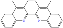
DMCH: 5,6-dihydro-4,7-dimethyl-dibenzo[3,2-b:2’3’-j]

$[1,10]$phenanthroline

OMCH: 4,7-dimethyldibenzo[3,1-b:2’,3’-j]

$[1,10]$phenanthroline

biq: 2,2’-biquinoline

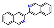
i-biq: 3,3’-biisoquinoline

Figure 22: Ligand list (part V).

BL4: 1,2-bis[4-(4’-methyl-2,2’-bipyridyl)]ethane

BL5: 1,5-bis[4-(4’-methyl-2,2’-bipyridyl)]pentane

BL6: 1,4,-bis[4-(4’-methyl-2,2’-bipyridyl)]benzene

BL7: 1,12-bis[4-r’-methyl-2,2’-bipyridyl)]dodecane

PMA: 2-aminomethylpyridine

Figure 23: Ligand list (part VI).

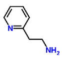
2-AEP: 2-(2-aminoethyl)pyridine

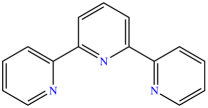
trpy: 2,2’;6’,2”-terpyridine

6-m-bpy: 6-methyl-2,2’-bipyridine

6,6’-dm-bpy: 6,6’-dimethyl-2,2’-bipyridine

2-m-phen: 2-methyl-1,10-phenanthroline

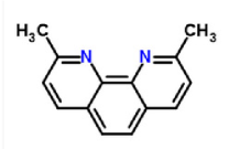
2,9-dm-phen: 2,9-dimethyl-1,10-phenanthroline

Figure 24: Ligand list (part VII).

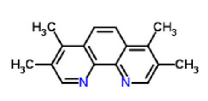
tm1-phen: 3,4,7,8-tetramethyl-1,10-phenanthroline

DPA: di-2-pyridylamine anion

DPAH: di-2-pyridylamine

Azpy: 2-(phenylazo)pyridine

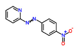
NA: 2-((4-nitrophenyl)azo)pyridine

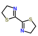
bt: 2,2’-bi-2-thiazoline

Figure 25: Ligand list (part VIII).

pynapy: 2-(2-pyridyl)-1,8-naphthyridine

dinapy: 5,6-dihydro-dipyrido[3,2-b:2’,3’-j]

$[1,10]$phenanthroline

tro: 4’-phenyl-2,2’,2”-tripyridine

tsite: 4,4’,4”-triphenyl-2,2’,2”-tripyridine

dqp: 2,6-di-(2’-quinolyl)pyridine

Figure 26: Ligand list (part IX).

References

- [1] D. E. Lewis, Klaus at Kazon: The Discovery of Ruthenium (1), Bull. Hist. Chem. 41, 3 (2016).
- [2] J. Sauvage et al., Ruthenium(II) and Osmium(II) bis(terpyridine) complexes in covalently-linked multicomponent systems: Synthesis, electrochemical behavior, absorption spectra, and photochemical and photophysical properties, Chem. Rev. 94, 993 (1994).
- [3] C. M. Wawire et al., Density-Functional Study of Lumininescence in Polypyridine Ruthenium Complexes, J. Photochem. and Photobiol. A 276, 8 (2014).
- [4] V. Balzani and A. Juris, Photochemistry and photophysics of Ru (II) polypyridine complexes in the Bologna group. From early studies to recent developments, Coordin. Chem. Rev. 211, 97 (2001).
- [5] K. Nakamaru, Synthesis, luminescence quantum yields, and lifetimes of trischelated ruthenium(II) mixed-ligand complexes including 3,3’-dimethyl-2,2’-bipyridyl, Bull. Chem. Soc. Jpn. 55, 2697 (1982).
- [6] G. Liebsch, I. Klimant, and O. S. Wolfbeis, Luminescence lifetime temperature sensing based on sol-gels and poly(acrylonitrile)s dyed with ruthenium metal-ligand complexes, Adv. Mat. 11, 1296 (1999).
- [7] A. Harriman, A. Khatyr, and R. Ziessel, Extending the luminescence lifetime of ruthenium(II) poly(pyridine) complexes in solution at ambient temperature, Dalton Trans. 10, 2061 (2003).
- [8] M. Duati et al., Enhancement of luminescence lifetimes of mononuclear ruthenium(II)-terpyridine complexes by manipulation of the -donor strength of ligands, J. Inorg. Chem. 42, 8377 (2003).
- [9] E. A. Medlycott and G. S. Hanan, Designing tridentate ligands for ruthenium(II) complexes with prolonged room temperature luminescence lifetimes, Chem. Soc. Rev. 34, 133 (2005).
- [10] K. J. Morris, M. S. Roach, W. Xu, J. N. Demas, and B. A. DeGraff, Luminescence lifetime standards for the nanosecond to microsecond range and oxygen quenching of ruthenium(II) compounds, Anal. Chem. 79, 9310 (2007).
- [11] L. J. Nurkkala et al., The effects of pendant vs. fused thiophene attachment upon the luminescence lifetimes and electrochemistry of tris(2,2’-bipyridine)ruthenium(II) complexes, Eur. J. Inorg. Chem. 26, 4101 (2008).
- [12] R. O. Steen et al., The role of isometric effects on the luminescence lifetimes and electrochemistry of oligothienyl-bridged dinuclear tris(2,2’-bipyridine)ruthenium(II) complexes, Eur. J. Inorg. Chem. 11, 1784 (2008).
- [13] S. Ji et al., Tuning the luminescence lifetimes of ruthenium(II) polypyridine complexes and its application in luminescent oxygen sensing, J. Mater. Chem. 20, 1953 (2010).
- [14] B. N. Figgis and M. A. Hitchman, Ligand Field Theory and Its Applications, Wiley-VCH, New York, 2000.
- [15] H. Ramanantoanina, W. Urland, A. Garciá-Fuente, F. Cimpoesu, and C. Daul, Ligand field density functional theory for the prediction of future domestic lighting, Phys. Chem. Chem. Phys. 28, 14625 (2014).
- [16] A. Juris et al., Ru(II) Polypyridine Complexes: Photophysics, Photochemistry, Electrochemistry, and Chemiluminescence, Coord. Chem. Rev. 84, 85 (1988).
- [17] M. Kasha, Characterization of electronic transitions in complex molecules, Discuss. Faraday Soc. 9, 14 (1950).
- [18] G. A. Crosby, Spectroscopic investigations of excited states of transition-metal complexes, Acc. Chem. Res. 8, 231 (1975).
- [19] V. Balazni and S. Campagna, editors, Photochemistry and Photophysics of Coordination Compounds. I., volume 280 of Top. Curr. Chem., Heidelberg, 2007, Springer.
- [20] V. Balazni and S. Campagna, editors, Photochemistry and Photophysics of Coordination Compounds. II., volume 281 of Top. Curr. Chem., Heidelberg, 2007, Springer.
- [21] F. Barigelletti, A. Juris, V. Balzani, P. Belser, and A. von Zelewsky, Temperature dependence of the Ru(bpy)2(CN)2 and Ru(bpy)2(i-biq)2+ luminescence, J. Phys. Chem. 91, 1095 (1987).
- [22] M. J. Frisch et al., Gaussian 03, Revision B.05, Gaussian, Inc.,Pittsburgh, PA, 2003.
- [23] M. J. Frisch et al., Gaussian∼09 Revision D.01.
- [24] W. Kohn and L. J. Sham, Self-consistent equations including exchange and correlation effects, Phys. Rev. 140, A1133 (1965).
- [25] A. D. Becke, Density-functional exchange-energy approximation with correct asymptotic behavior, Phys. Rev. A 38, 3098 (1988).
- [26] S. H. Vosko, L. Wilk, and M. Nusair, Accurate spin-dependent electron liquid correlation energies for local spin density calculations: a critical analysis, Can. J. Phys. 58, 1200 (1980).
- [27] C. Lee, W. Yang, and R. G. Parr, Development of the Colle-Salvetti correlation-energy formula into a functional of the electron density, Phys. Rev. B 37, 785 (1988).
- [28] A. D. Becke, Density-functional thermochemistry. III. The role of exact exchange., J. Chem. Phys. 98, 5648 (1993).
- [29] P. J. Hay and W. R. Wadt, Ab initio effective core potentials for molecular calculations. potentials for K to Au including the outermost core orbitals, J. Chem. Phys. 82, 299 (1985).
- [30] P. J. Hay and W. R. Wadt, Ab initio effective core potentials for molecular calculations. Potentials for the transition metal atoms Sc to Hg, J. Chem. Phys. 82, 270 (1985).
- [31] R. Ditchfield, W. Hehre, and J. A. Pople, Self-consistent molecular-orbital methods. IX. An extended Gaussian-type basis for molecular-orbital studies of organic molecules, J. Chem. Phys. 54, 724 (1971).
- [32] W. J. Hehre, R. Ditchfield, and J. A. Pople, Self-consistent molecular orbital methods. XII. Further extensions of Gaussian-type basis sets for use in molecular orbital studies of organic molecules, J. Chem. Phys. 56, 2257 (1972).
- [33] P. Hariharan and J. A. Pople, The influence of polarization functions on molecular orbital hydrogenation energies, Theor. Chim. Acta 28, 213 (1973).
- [34] P. C. Hariharan and J. A. Pople, Accuracy of AHn equilibrium geometries by single determinant molecular orbital theory, Mol. Phys. 27, 209 (1974).
- [35] M. M. Francl et al., Self-consistent molecular orbital methods. XXIII. A polarization-type basis set for second-row elements, J. Chem. Phys. 77, 3654 (1982).
- [36] V. A. Rassolov, M. A. Ratner, J. A. Pople, P. C. Redfern, and L. A. Curtiss, 6-31G* basis set for third-row atoms, J. Comp. Chem. 22, 976 (2001).
- [37] G. A. Petersson and M. A. Al-Laham, A complete basis set model chemistry. II. Open-shell systems and the total energies of the first-row atoms, J. Chem. Phys. 94, 6081 (1991).
- [38] The Cambridge Crystallographic Data Centre (CCDC), https://www.ccdc.cam.ac.uk/, Last accessed: 6 February 2016.
- [39] R. Prajapati, V. K. Yadav, S. K. Dubey, B. Durham, and L. Mishra, CCDC 667743: Experimental Crystal Structure Determination, DOI: 10.5517/ccqdv31, 2007.
- [40] R. Prajapati, V. K. Yadav, S. K. Dubey, B. Durham, and L. Mishra, Reactivity of metal (ZnII, RuII)-2,2’-bipyridyl with some bifunctional ligands, Indian J. Chem., Sect. A 47, 1780 (2008).
- [41] O. S. Odongo, J. F. Endicott, and M. J. Heeg, CCDC 613874: Experimental Crystal Structure Determination, DOI: 10.5517/ccnlsdd, 2006.
- [42] F. R. Fronczek, CCDC 287967: Experimental Crystal Structure Determination, DOI: 10.5517/cc9nn8v, 2005.
- [43] H. Shen et al., A new three-dimensional ruthenium(II) complex via hydrogen bonds: Ru(bpy)2(ox)4H2O (bpy= 2,2′-bipyridine, ox= oxalate ion), Inorg. Chem. Commun. 2, 615 (1999).
- [44] D. P. Rillema, D. S. Jones, and H. A. Levy, Structure of tris(2,2-bipyridyl)ruthenium(II) hexafluorophosphate, [Ru(bipy)3][PF6]2; X-ray crystallographic determination, J. Chem. Soc. Chem. Commun. 1979, 849 (1979).
- [45] P. Reveco, R. H. Schmehl, W. R. Cherry, F. R. Froczek, and J. Selbin, Cyclometalated complexes of ruthenium. 2. Spectral and electrochemical properties and x-ray structure of bis(2,2’-bipyridine)(4-nitro-2-(2-pyridyl)phenyl)ruthenium(II), Inorg. Chem. 24, 4078 (1985).
- [46] D. Hesek et al., CCDC 116354: Experimental Crystal Structure Determination, DOI: 10.5517/cc3x2cf, 1999.
- [47] D. Hesek et al., Conversion of a new chiral reagent -[Ru(bpy)2(dmso)Cl]PF6 to -[Ru(bpy)2(dmbpy)]PF6Cl with 96.8% retention of chirality (dmbpy = 4,4]’-dimethyl-2,2’-bipyridine), Chem. Commun. 5, 403 (1999).
- [48] L. E. Hansen et al., CCDC 212499: Experimental Crystal Structure Determination, DOI: 10.5517/cc743t8, 2003.
- [49] L. E. Hansen et al., Syntheses and characterization of some chloro, methoxy, and mercapto derivatives of [Ru(-2,2’-bipyridine)3]2+2PF: crystal and molecular structures of [Ru(-2,2’-bipyridine)2(-4,4’-(X)2-2,2’-bipyridine)]2+2PF (X=Cl, OCH3), Inorg. Chim. Acta 348, 91 (2003).
- [50] M. Du, X. Ge, H. Liu, and X. Bu, CCDC 169415: Experimental Crystal Structure Determination, DOI: 10.5517/cc5p904, 2001.
- [51] M. Du, X. Ge, H. Liu, and X. Bu, Synthesis, spectra, and crystal structures of two Ru complexes with polypyridyl ligands: cis-[Ru(pby)2(4,4’-bpy)Cl](PF6)H2O and cis-[Ru(phen)2(CH3CN)2](PF6)2, J. Mol. Struct. 610, 207 (2002).
- [52] B. Ye, X. Chen, T. Zeng, and L. Ji, syntheses, spectra and crystal structures of ruthenium(II) complexes with polypyridyl:[Ru(bipy)2(phen)](ClO4)2.H2O and [Ru(bipy)2 (Me-phen)](ClO, Inorg. Chim. Acta 240, 5 (1995).
- [53] V. W. Yam, B. Li, and N. Zhu, CCDC 182310: Experimental Crystal Structure Determination, DOI: 10.5517/cc63pzy, 2002.
- [54] V. W. Yam, B. Li, and N. Zhu, Synthesis of Mesoporous Silicates with Controllable Pore Size Using Surfactant Ruthenium(II) Complexes as Templates, Adv. Mater. 14, 719 (2002).
- [55] C. M. Kepert et al., CCDC 230551: Experimental Crystal Structure Determination, DOI: 10.5517/cc7qx4z, 2004.
- [56] C. M. Kepert et al., The synthesis and structure of heteroleptic tris(diimine)ruthenium(II) complexes, Dalton Trans. , 1766 (2004).
- [57] L. J. Henderson Jr., F. R. Fronczek, and W. R. Cherry, Selective perturbation of ligand field excited states in polypyridine ruthenium(II) complexes, J. Am. Chem. Soc. 106, 5876 (1984).
- [58] Y. Wang, D. C. Jackman, C. Woods, and D. P. Rillema, Crystal structure, physical, and photophysical properties of a ruthenium (II) bipyridine diazafluorenone complex, J. Chem. Crystallogr. 25, 549 (1995).
- [59] P. B. Hitchcock et al., Cis-bis(2,2’-bipyridine)bis(pyridine)ruthenium(II), J. Chem. Soc., Dalton Trans. 1988, 1837 (1988).
- [60] B. Klop, H. Viebrock, A. von Zelewsky, and D. Abeln, CCDC 162056: Experimental Crystal Structure Determination, DOI: 10.5517/cc5fmmt, 2001.
- [61] B. Klop, H. Viebrock, A. von Zelewsky, and D. Abeln, Crystal Structure Analysis and Chiral Recognition Study of -[Ru(bpy)2(py)2][(+)-O,O’-dibenzoyl-D-tatrate]12H2O and -[Ru(bpy)2(py)2][(-)-O,O’-dibenzoyl-L-tatrate]12H2O, Inorg. Chem. 40, 1196 (2001).
- [62] A. H. Velders et al., CCDC 143552: Experimental Crystal Structure Determination, DOI: 10.5517/cc4tcq0, 2000.
- [63] A. H. Velders et al., A simple example of the fluxional behaviour of ruthenium-coordinated -symmetric monodentate ligands – synthesis 1H NMR spectroscopic study and crystal structure of cis-[Ru(bpy)2(4Pic)2](PF6)2, Eur. J. Inorg. Chem. 2002, 193 (2002).
- [64] S. Derossi, H. Adams, and M. D. Ward, CCDC 622792: Experimental Crystal Structure Determination, DOI: 10.5517/ccnx22p, 2006.
- [65] S. Derossi, H. Adams, and M. D. Ward, Hydrogen-bonded assemblies of ruthenium(II)-biimidazole complex cations and cyanometallate anions: structures and photophysics, Dalton Trans. 2007, 33 (2007).
- [66] N. Rockstroh et al., CCDC 760286: Experimental Crystal Structure Determination, DOI: 10.5517/cctj4ct, 2010.
- [67] N. Rockstroh et al., Structural properties of ruthenium biimidazole complexes determining the stability of their supramolecular aggregates, Z. Naturforsch., B: Chem. Sci 65, 281 (2010).
- [68] P. Wang et al., Structure and properties of diastereoisomers of a ruthenium(II) complex having a pyridylpyrazoline derivative as a ligand, Chem. Lett. 30, 940 (2001).
- [69] A. A. Farah, D. V. Stynes, and W. J. Pietro, CCDC 140838: Experimental Crystal Structure Determination, DOI: 10.5517/cc4qk5k, 2000.
- [70] A. A. Farah, D. V. Stynes, and W. J. Pietro, Syntheses, characterization and structures of 2-(2-pyridyl)-4-methylcarboxyquinoline ligand and bis(2,2-bipyridine)-2-(2-pyridyl)-4-methylcarboxyquinoline ruthenium(II) hexafluorophosphate, Inorg. Chim. Acta 343, 295 (2003).
- [71] S. Rau et al., CCDC 236778: Experimental Crystal Structure Determination, DOI: 10.5517/cc7yd0k, 2004.
- [72] S. Rau et al., Efficient synthesis of ruthenium complexes of the type (R-bpy)2RuCl2 and [(R-bpy)2Ru(L-L)]Cl by microwave-activated reactions (R: H, Me, tert-But) (L-L: substituted bibenzimidazoles, bipyrimidine, and phenanthroline), Inorg. Chim. Acta 357, 4496 (2004).
- [73] P. U. Maheswari, V. Rajendiran, M. Palaniandavar, R. Thomas, and G. U. Kulkarni, CCDC 623203: Experimental Crystal Structure Determination, DOI: 10.5517/ccnxhbc, 2006.
- [74] P. U. Maheswari, V. Rajendiran, M. Palaniandavar, R. Thomas, and G. U. Kulkarni, Mixed ligand ruthenium(II) complexes of 5,6-dimethyl-1,10-phenanthroline: the role of ligand hydrophobicity on DNA binding of the complexes, Inorg. Chim. Acta 359, 4601 (2006).
- [75] M. Kato, K. Sasano, M. Kimura, and S. Yamauchi, Solid state effect on the phosphorescence spectrum of a tris(3,3’-biisoquinoline)ruthenium(II) salt, Chem. Lett. 21, 1887 (1992).
- [76] A. Taketoshi, T. Koizumi, and T. Kanbara, CCDC 789502: Experimental Crystal Structure Determination, DOI: 10.5517/ccvhjtn, 2010.
- [77] A. Taketoshi, T. Koizumi, and T. Kanbara, Aerobic oxidative dehydrogenation of benzylamines catalyzed by cyclometalated ruthenium complex, Tetrahedron Lett. 51, 6457 (2010).
- [78] C. Tsai et al., Characterization of low energy charge transfer transitions in (terpyridine)(bipyridine)ruthenium(II) complexes and their cyanide-bridge bi- and tri-metallic analogues, Inorg. Chem. 50, 11965 (2011).
- [79] C. Tsai et al., CCDC 868664: Experimental Crystal Structure Determination, DOI: 10.5517/ccy4xfd, 2012.
- [80] D. Onggo, M. L. Scudder, D. C. Craig, and H. A. Goodwin, CCDC 222020: Experimental Crystal Structure Determination, DOI: 10.5517/cc7g0ym, 2003.
- [81] D. Onggo, M. L. Scudder, D. C. Craig, and H. A. Goodwin, The influence of ortho-substitution within the ligand on the geometry of the tris(2,2′-bipyridine)ruthenium(II) and tris(1,10-phenanthroline)ruthenium(II) ions, J. Molec. Struc. 738, 129 (2005).
- [82] M. Schwalbe et al., CCDC 614185: Experimental Crystal Structure Determination, DOI: 10.5517/ccnm3fs, 2006.
- [83] M. Schwalbe et al., Synthesis and characterisation of poly(bipyridine)ruthenium complexes as building blocks for heterosupramolecular arrays, Euro. J. Inorg. Chem. 2008, 3310 (2008).
- [84] D. Onggo, M. L. Scudder, D. C. Craig, and H. A. Goodwin, CCDC 222021: Experimental Crystal Structure Determination, DOI: 10.5517/cc7g0zn, 2003.
- [85] J. Gao et al., CCDC 900121: Experimental Crystal Structure Determination, DOI: 10.5517/ccz6n5z, 2012.
- [86] J. Gao et al., Molecule-based water-oxidation catalysts (WOCs): Cluster-size-dependent dye-sensitized polyoxometalates for visible-light-driven O2 evolution, Sci. Rep. 3, 1853 (2013).
- [87] E. Baranoff et al., CCDC 182680: Experimental Crystal Structure Determination, DOI: 10.5517/cc642x9, 2002.
- [88] E. Baranoff et al., Photochemical or thermal chelate exchange in the ruthenium coordination sphere of complexes of the Ru(phen)2L family (L = diimine or dinitrile ligands), Inorg. Chem. 41, 1215 (2002).
- [89] E. Wachter, D. K. Heidary, B. S. Howerton, S. Parkin, and E. C. Glazer, CCDC 881148: Experimental Crystal Structure Determination, DOI: 10.5517/ccykx4j, 2012.
- [90] E. Wachter, D. K. Heidary, B. S. Howerton, S. Parkin, and E. C. Glazer, Light-activated ruthenium complexes photo bind DNA and are cytotoxic in the photodynamic therapy window, Chem. Commun. 48, 9649 (2012).
- [91] D. Onggo, M. L. Scudder, D. C. Craig, and H. A. Goodwin, CCDC 222019: Experimental Crystal Structure Determination, DOI: 10.5517/cc7g0xl, 2003.
- [92] A. C. G. Hotze et al., CCDC 251699: Experimental Crystal Structure Determination, DOI: 10.5517/cc8fxbx, 2004.
- [93] A. C. G. Hotze et al., Characterization by NMR Spectroscopy, X-ray Analysis and Cytotoxic Activity of the Ruthenium(II) Compounds [RuL3](PF6)2 (L = 2-Phenylazopyridine or o-Tolylazopyridine) and [RuL’2L”](PF6)2 (L’, L” = 2-Phenylazopyridine, 2,2’-Bipyridine), Eur. J. Inorg. Chem. 2005, 2648 (2005).
- [94] A. A. Farah and W. J. Pietro, CCDC 199681: Experimental Crystal Structure Determination, DOI: 10.5517/cc6psbz, 2002.
- [95] A. A. Farah and W. J. Pietro, Synthesis, structure and electrochemical properties of tris(2-(2-pyridyl)-4-methylcarbonylquinoline)ruthenium(II) hexafluorophosphate, Inorg. Chem. Comm. 6, 662 (2003).
- [96] M. Kozlowska, P. Rodziewicz, D. M. Brus, J. Breczko, and K. Brzezinski, CCDC 909756: Experimental Crystal Structure Determination, DOI: 10.5517/cczjnz3, 2012.
- [97] M. Kozlowska, P. Rodziewicz, D. M. Brus, J. Breczko, and K. Brzezinski, Bis (2, 2′: 6′, 2′′-terpyridine) ruthenium (II) bis (perchlorate) hemihydrate, Acta Crystallogr. Sect. E: Struct. Rep. Online 68, 1414 (2012).
- [98] E. C. Constable et al., CCDC 676373: Experimental Crystal Structure Determination, DOI: 10.5517/ccqpthp, 2008.
- [99] E. C. Constable et al., Bis(4’-phenyl-2,2’:6’,2”-terpyridine)ruthenium(II): Holding the embraces at bay, Inorg. Chem. Comm. 11, 805 (2008).
- [100] F. H. Allen, The Cambridge Structural Database: a quarter of a million crystal structures and rising, Acta Crystallogr. B 58, 380 (2002).
- [101] R. Dennington, T. Keith, and J. Millam, GaussView Version 5, Semichem Inc. Shawnee Mission KS 2009.
- [102] M. E. Casida, Time-dependent density-functional theory for molecules and molecular solids, J. Molec. Struct.: THEOCHEM 914, 3 (2009).
- [103] M. E. Casida and M. Huix-Rotllant, Progress in Time-Dependent Density-Functional Theory, Annu. Rev. Phys. Chem. 63, 287 (2012).
- [104] A. A. M. H. M. Darghouth et al., Assessment of Density-Functional Tight-Binding Ionization Potentials and Electron Affinities of Molecules of Interest for Organic Solar Cells Against First-Principles Calculations, Computation 3, 616 (2015).
- [105] W. Koch and M. C. Holtzhausen, A Chemist’s Guide to Density Functional Theory, Wiley-VCH, New York, 2000.
- [106] N. Yoshikawa et al., Transition states of the 3 MLCT to 3 MC conversion in Ru (bpy)2(phen derivative) 2+ complexes, J. Mol. Struct. 1094, 98 (2015).
- [107] E. Borfecchia et al., X-ray transient absorption structural characterization of the 3MLCT triplet excited state of cis-[Ru(bpy)2(py)2]2+, Dalton Trans. 42, 6564 (2013).
- [108] J. Y. Choi, E. J. Park, S. H. Chang, and T. J. Kang, Solvent effects on the solvatochromism of 7-aminocoumarin derivatives in neat and binary solvent mixtures: Correlation of the electronic transition energies with the solvent polarity parameters, Bull. Korean Chem. Soc. 30, 1452 (2009).
- [109] M. Maestri, N. Armaroli, V. Blazani, E. C. Constable, and A. M. W. C. Thompson, Complexes of the Ruthenium(II)-2,2’;6’,2”-terpyridine Family. Effect of Electron-Accepting and Donating Substituents on the Photophysical and Electrochemical Properties, Inorg. Chem. 34, 2759 (1995).
- [110] F. Barigelletti, P. Belser, A. von Zelewsky, A. Juris, and V. Balzani, Luminescence of mixed-ligand polypyridine-ruthenium(II) complexes in the temperature range 84-250 K. Interligand interactions and viscosity effects on radiationless processes, J. Phys. Chem. 89, 3680 (1985).
- [111] I. Fleming, Frontier Orbitals and Organic Chemical Reactions, John Wiley and Sons, New York, 1976.
- [112] N. T. Anh, Frontier Orbitals: A Practical Manual, John Wiley and Sons, The Atrium, Soutern Gate, Chichester, West Sussex PO19 8SQ, England, 2007.
- [113] M. J. S. Dewar, A Critique of Frontier Orbital Theory, THEOCHEM 200, 301 (1989).
- [114] M. Wolfsberg and L. Helmholtz, The spectra and electronic structure of the tetrahedral ions MnO, CrO, and ClO, J. Chem. Phys. 20, 837 (1952).
- [115] C. Daniel, Electronic spectroscopy and photoreactivity in transition metal complexes, Coord. Chem. Rev. 238-239, 143 (2003).
- [116] A. Rosa, G. Ricciardi, O. Gritsenko, and E. J. Baerends, Excitation energies of metal complexes with time-dependent density functional theory, Stuct. Bond. 112, 49 (2004).
- [117] A. V. Jr. and S. Záliš, Modeling of charge-transfer transitions and excited states in transition metal complexes by DFT techniques, Coord. Chem. Rev. 251, 258 (2007).