Lipschitz stability for an inverse hyperbolic problem of determining two coefficients by a finite number of observations

L. Beilina Department of Mathematical Sciences, Chalmers University of Technology and University of Gothenburg, SE-42196 Gothenburg, Sweden, e-mail:  larisa@chalmers.se    M. Cristofol Institut de Mathématiques de Marseille, CNRS, UMR 7373, École Centrale, Aix-Marseille Université, 13453 Marseille, France, e-mail:  michel.cristofol@univ-amu.fr    S. Li Key Laboratory of Wu Wen-Tsun Mathematics, Chinese Academy of Sciences, School of Mathematical Sciences, University of Science and Technology of China, 96 Jinzhai Road, Hefei, Anhui Province, 230026, China, e-mail:  shuminli@ustc.edu.cn    M. Yamamoto Department of Mathematical Sciences, The University of Tokyo, Komaba, Meguro, Tokyo 153, Japan, e-mail: myama@ms.u-tokyo.ac.jp
Abstract

We consider an inverse problem of reconstructing two spatially varying coefficients in an acoustic equation of hyperbolic type using interior data of solutions with suitable choices of initial condition. Using a Carleman estimate, we prove Lipschitz stability estimates which ensures unique reconstruction of both coefficients. Our theoretical results are justified by numerical studies on the reconstruction of two unknown coefficients using noisy backscattered data.

1 Statement of the problem

1.1 Introduction

The main purpose of this paper is to study the inverse problem of determining simultaneously the function ρ(x)𝜌𝑥\rho(x) and the conductivity p(x)𝑝𝑥p(x) in the following:

ρ(x)t2udiv(p(x)u)=0𝜌𝑥superscriptsubscript𝑡2𝑢div𝑝𝑥𝑢0\rho(x)\partial_{t}^{2}u-\mathrm{div}\,(p(x)\nabla u)=0 (1.1)

from a finite number of boundary observations on the domain ΩΩ\Omega which is a bounded open subset of n,n1superscript𝑛𝑛1\mathbb{R}^{n},\;n\geq 1.

The reconstruction of two coefficients of the principal part of an operator with a finite number of observations is very challenging since we mix at least two difficulties, see [15] for the case of a principal matrix term in the divergence form, arising from anisotropic media) or [25] for Lame system or [6, 13, 38, 39, 40] for Maxwell system.

Furthermore, in this work we establish a Lipschitz stability inequality. First, this stability inequality implies the uniqueness of the reconstruction of coefficients ρ(x)𝜌𝑥\rho(x) and p(x)𝑝𝑥p(x). Second, we can use it to perform numerical reconstruction with noisy observations to be more close to real-life applications.

Bukhgeim and Klibanov [19] created the methodology by Carleman estimate for proving the uniqueness in coefficient inverse problems and after [19], there has been many works published on this topic. We refer to some of them. [11, 12, 15, 16, 17], [26] - [28], [32] - [34], [37, 48]. In all these works except the recent works [5, 6], only theoretical studies are presented. From other side, the existence of a stability theorems allow us to improve the results of the numerical reconstruction by choosing different regularization strategies in the minimization procedure.

In particular we refer to Imanuvilov and Yamamoto [27] which established the Lipschitz stability for the coefficient inverse problem for a hyperbolic equation. Our argument in this paper is a simplification of [27] and Klibanov and Yamamoto [37].

To the authors’ knowledge, there exist few works which study numerical reconstruction based on the theoretical stability analysis for the inverse problem with finite and restricted measurements. Furthermore, the case of the reconstruction of the conductivity coefficient in the divergence form for the hyperbolic operator induces some numerical difficulties, see [3, 7, 10, 22] for details.

In numerical simulations of this paper we use similar optimization approach which was applied recently in works [3, 5, 6, 8, 10]. More precisely, we minimize the Tikhonov functional in order to reconstruct unknown spatially distributed wave speed and conductivity functions of the acoustic wave equation from transmitted or backscattered boundary measurements. For minimization of the Tikhonov functional we construct the associated Lagrangian and minimize it on the adaptive locally refined meshes using the domain decomposition finite element/finite difference method similar to one of [3]. Details of this method can be found in forthcoming publication. The adaptive optimization method is implemented efficiently in the software package WavES [47] in C++/PETSc [45].

Our numerical simulations show that we can accurately reconstruct location of both space-dependent wave speed and conductivity functions already on a coarse non-refined mesh. The contrast of the conductivity function is also reconstructed correctly. However, the contrast of the wave speed function should be improved. In order to obtain better contrast, similarly with [2, 7, 8], we applied an adaptive finite element method, and refined the finite element mesh locally only in places, where the a posteriori error of the reconstructed coefficients was large. Our final results attained on a locally refined meshes show that an adaptive finite element method significantly improves reconstruction obtained on a coarse mesh.

The outline of this paper is as follows. In Section 2, we show a key Carleman estimate, in Section 3 we complete the proofs of Theorems 1.1 and 1.2. Finally, in section 4 we present numerical simulations taking into account the theoretical observations required in Theorem 1.1 as an important guidance. Section 5 concludes the main results of this paper.

1.2 Settings and main results

Let ΩnΩsuperscript𝑛\Omega\subset\mathbb{R}^{n} be a bounded domain with smooth boundary ΩΩ\partial\Omega. We consider an acoustic equation

ρ(x)t2u(x,t)div(p(x)u(x,t))=0,xΩ, 0<t<T.formulae-sequence𝜌𝑥superscriptsubscript𝑡2𝑢𝑥𝑡div𝑝𝑥𝑢𝑥𝑡0formulae-sequence𝑥Ω 0𝑡𝑇\rho(x)\partial_{t}^{2}u(x,t)-\mbox{div}\thinspace(p(x)\nabla u(x,t))=0,\quad x\in\Omega,\thinspace 0<t<T. (1.2)

To (1.2) we attach the initial and boundary conditions:

u(x,0)=a(x),tu(x,0)=0,xΩformulae-sequence𝑢𝑥0𝑎𝑥formulae-sequencesubscript𝑡𝑢𝑥00𝑥Ωu(x,0)=a(x),\quad\partial_{t}u(x,0)=0,\quad x\in\Omega (1.3)

and

u(x,t)=h(x,t),(x,t)Ω×(0,T).formulae-sequence𝑢𝑥𝑡𝑥𝑡𝑥𝑡Ω0𝑇u(x,t)=h(x,t),\quad(x,t)\in\partial\Omega\times(0,T). (1.4)

We will write u(p,ρ,a,h)𝑢𝑝𝜌𝑎u(p,\rho,a,h) a weak solution of the problem (1.2)-(1.4). Functions p,ρ𝑝𝜌p,\rho are assumed to be positive on Ω¯¯Ω\overline{\Omega} and are unknown in ΩΩ\Omega. They should be determined by extra data of solutions u𝑢u in ΩΩ\Omega.

Throughout this paper, we set j=xjsubscript𝑗subscript𝑥𝑗\partial_{j}=\frac{\partial}{\partial x_{j}}, ij=2xixjsubscript𝑖subscript𝑗superscript2subscript𝑥𝑖subscript𝑥𝑗\partial_{i}\partial_{j}=\frac{\partial^{2}}{\partial x_{i}\partial x_{j}}, t2=2t2superscriptsubscript𝑡2superscript2superscript𝑡2\partial_{t}^{2}=\frac{\partial^{2}}{\partial t^{2}}, 1i,jnformulae-sequence1𝑖𝑗𝑛1\leq i,j\leq n.

Let ωΩ𝜔Ω\omega\subset\Omega be a suitable subdomain of ΩΩ\Omega and T>0𝑇0T>0 be given. In this paper, we consider an inverse problem of determining coefficients p=p(x)𝑝𝑝𝑥p=p(x) and ρ=ρ(x)𝜌𝜌𝑥\rho=\rho(x) of the principal term, from the interior observations:

u(x,t),xω, 0<t<T.formulae-sequence𝑢𝑥𝑡𝑥𝜔 0𝑡𝑇u(x,t),\quad x\in\omega,\thinspace 0<t<T.

In order to formulate our results, we need to introduce some notations. For sufficiently smooth positive coefficients p𝑝p and ρ𝜌\rho and initial and boundary data, we can prove the existence of a unique weak solution to (1.2)-(1.4) (e.g., Lions and Magenes [42]), which we denote by u=u(p,ρ,a,h)𝑢𝑢𝑝𝜌𝑎u=u(p,\rho,a,h).

Henceforth (,)(\cdot,\cdot) denotes the scalar product in nsuperscript𝑛\mathbb{R}^{n}, and ν=ν(x)𝜈𝜈𝑥\nu=\nu(x) be the unit outward normal vector to ΩΩ\partial\Omega at x𝑥x. Let the subdomain ωΩ𝜔Ω\omega\subset\Omega satisfy

ω{xΩ;((xx0)ν(x)))>0}\partial\omega\supset\{x\in\partial\Omega;\thinspace((x-x_{0})\cdot\nu(x)))>0\} (1.5)

with some x0Ω¯subscript𝑥0¯Ωx_{0}\not\in\overline{\Omega}. We note that ωΩ𝜔Ω\omega\subset\Omega cannot be an arbitrary subdomain. For example, in the case of a ball ΩΩ\Omega, the condition (1.5) requires that ω𝜔\omega should be a neighborhood of a sub-boundary which is larger than the half of ΩΩ\partial\Omega. The condition (1.5) is also a sufficient condition for an observability inequality by observations in ω×(0,T)𝜔0𝑇\omega\times(0,T) (e.g., Ch VII, section 2.3 in Lions [41]).

We set

Λ=(supxΩ|xx0|2infxΩ|xx0|2)12.Λsuperscriptsubscriptsupremum𝑥Ωsuperscript𝑥subscript𝑥02subscriptinfimum𝑥Ωsuperscript𝑥subscript𝑥0212\Lambda=\left(\sup_{x\in\Omega}|x-x_{0}|^{2}-\inf_{x\in\Omega}|x-x_{0}|^{2}\right)^{\frac{1}{2}}. (1.6)

We define admissible sets of unknown coefficients. For arbitrarily fixed functions η0C2(Ω¯)subscript𝜂0superscript𝐶2¯Ω\eta_{0}\in C^{2}(\overline{\Omega}), η1(C2(Ω¯))nsubscript𝜂1superscriptsuperscript𝐶2¯Ω𝑛\eta_{1}\in(C^{2}(\overline{\Omega}))^{n} and constants M1>0,0<θ01,θ1>0formulae-sequenceformulae-sequencesubscript𝑀100subscript𝜃01subscript𝜃10M_{1}>0,0<\theta_{0}\leq 1,\theta_{1}>0, we set

𝒰1=𝒰M1,θ1,η0,η11={pC2(Ω¯);p=η0,p=η1on Ω,\mathcal{U}^{1}=\mathcal{U}^{1}_{M_{1},\theta_{1},\eta_{0},\eta_{1}}=\biggl{\{}p\in C^{2}(\overline{\Omega});\thinspace p=\eta_{0},\thinspace\nabla p=\eta_{1}\quad\mbox{on $\partial\Omega$}, (1.7)
pC2(Ω¯)M1,pθ1on Ω¯},\displaystyle\|p\|_{C^{2}(\overline{\Omega})}\leq M_{1},\quad p\geq\theta_{1}\quad\mbox{on $\overline{\Omega}$}\biggr{\}},
𝒰2=𝒰M1,θ12={ρC2(Ω¯);ρC2(Ω¯)M1,ρθ1on Ω¯},superscript𝒰2subscriptsuperscript𝒰2subscript𝑀1subscript𝜃1formulae-sequence𝜌superscript𝐶2¯Ωformulae-sequencesubscriptnorm𝜌superscript𝐶2¯Ωsubscript𝑀1𝜌subscript𝜃1on Ω¯\displaystyle\mathcal{U}^{2}=\mathcal{U}^{2}_{M_{1},\theta_{1}}=\biggl{\{}\rho\in C^{2}(\overline{\Omega});\thinspace\|\rho\|_{C^{2}(\overline{\Omega})}\leq M_{1},\quad\rho\geq\theta_{1}\quad\mbox{on $\overline{\Omega}$}\biggr{\}},
𝒰=𝒰M1,θ0,θ1,η0,η1,x0={(p,ρ)𝒰1×𝒰2;((pρ1)(xx0))2pρ1(x)<1θ0,xΩω¯}.𝒰subscript𝒰subscript𝑀1subscript𝜃0subscript𝜃1subscript𝜂0subscript𝜂1subscript𝑥0formulae-sequence𝑝𝜌superscript𝒰1superscript𝒰2formulae-sequence𝑝superscript𝜌1𝑥subscript𝑥02𝑝superscript𝜌1𝑥1subscript𝜃0𝑥¯Ω𝜔\displaystyle\mathcal{U}=\mathcal{U}_{M_{1},\theta_{0},\theta_{1},\eta_{0},\eta_{1},x_{0}}=\biggl{\{}(p,\rho)\in\mathcal{U}^{1}\times\mathcal{U}^{2};\quad\frac{(\nabla(p\rho^{-1})\cdot(x-x_{0}))}{2p\rho^{-1}(x)}<1-\theta_{0},\quad x\in\overline{\Omega\setminus\omega}\biggr{\}}.

We note that there exists a constant M0>0subscript𝑀00M_{0}>0 such that (pρ)C(Ω¯)M0subscriptnorm𝑝𝜌𝐶¯Ωsubscript𝑀0\left\|\nabla\left(\frac{p}{\rho}\right)\right\|_{C(\overline{\Omega})}\leq M_{0} for each (p,ρ)𝒰1×𝒰2𝑝𝜌superscript𝒰1superscript𝒰2(p,\rho)\in\mathcal{U}^{1}\times\mathcal{U}^{2}.

Then we choose a constant β>0𝛽0\beta>0 such that

β+M0Λθ1β<θ0θ1,θ1infxΩ|xx0|2βΛ2>0.formulae-sequence𝛽subscript𝑀0Λsubscript𝜃1𝛽subscript𝜃0subscript𝜃1subscript𝜃1subscriptinfimum𝑥Ωsuperscript𝑥subscript𝑥02𝛽superscriptΛ20\beta+\frac{M_{0}\Lambda}{\sqrt{\theta_{1}}}\sqrt{\beta}<\theta_{0}\theta_{1},\quad\theta_{1}\inf_{x\in\Omega}|x-x_{0}|^{2}-\beta\Lambda^{2}>0. (1.8)

Here we note that such β>0𝛽0\beta>0 exists by x0Ω¯subscript𝑥0¯Ωx_{0}\not\in\overline{\Omega}, and in fact β>0𝛽0\beta>0 should be sufficiently small.

We are ready to state our first main result.

Theorem 1.1.

Let q𝒰1𝑞superscript𝒰1q\in\mathcal{U}^{1} be arbitrarily fixed and let a1,a2C3(Ω¯)subscript𝑎1subscript𝑎2superscript𝐶3¯Ωa_{1},a_{2}\in C^{3}(\overline{\Omega}) satisfy

{|div(qa)|>0,=1 or =2,((div(qa2)a1div(qa1)a2)(xx0))>0on Ω¯.casesmissing-subexpressiondiv𝑞subscript𝑎0=1 or =2,missing-subexpressiondiv𝑞subscript𝑎2subscript𝑎1div𝑞subscript𝑎1subscript𝑎2𝑥subscript𝑥00on Ω¯\left\{\begin{array}[]{rl}&|\mbox{div}\thinspace(q\nabla a_{\ell})|>0,\quad\mbox{$\ell=1$ or $\ell=2$,}\\ &((\mbox{div}\thinspace(q\nabla a_{2})\nabla a_{1}-\mbox{div}\thinspace(q\nabla a_{1})\nabla a_{2})\cdot(x-x_{0}))>0\quad\mbox{on $\overline{\Omega}$}.\end{array}\right. (1.9)

We further assume that

u(q,σ,a,h)W4,(Ω×(0,T)),=1,2formulae-sequence𝑢𝑞𝜎subscript𝑎subscriptsuperscript𝑊4Ω0𝑇12u(q,\sigma,a_{\ell},h_{\ell})\in W^{4,\infty}(\Omega\times(0,T)),\quad\ell=1,2

and

T>Λβ.𝑇Λ𝛽T>\frac{\Lambda}{\sqrt{\beta}}. (1.10)

Then there exists a constant C>0𝐶0C>0 depending on Ω,T,𝒰,q,σΩ𝑇𝒰𝑞𝜎\Omega,T,\mathcal{U},q,\sigma and a constant M2>0subscript𝑀20M_{2}>0 such that

pqH1(Ω)+ρσL2(Ω)C=12u(p,ρ,a,h)u(q,σ,a,h)H3(0,T;L2(ω))subscriptnorm𝑝𝑞superscript𝐻1Ωsubscriptnorm𝜌𝜎superscript𝐿2Ω𝐶superscriptsubscript12subscriptnorm𝑢𝑝𝜌subscript𝑎subscript𝑢𝑞𝜎subscript𝑎subscriptsuperscript𝐻30𝑇superscript𝐿2𝜔\|p-q\|_{H^{1}(\Omega)}+\|\rho-\sigma\|_{L^{2}(\Omega)}\leq C\sum_{\ell=1}^{2}\|u(p,\rho,a_{\ell},h_{\ell})-u(q,\sigma,a_{\ell},h_{\ell})\|_{H^{3}(0,T;L^{2}(\omega))} (1.11)

for each (p,ρ)𝒰𝑝𝜌𝒰(p,\rho)\in\mathcal{U} satisfying

u(p,ρ,a,h)W4,(Ω×(0,T))M2.subscriptnorm𝑢𝑝𝜌subscript𝑎subscriptsuperscript𝑊4Ω0𝑇subscript𝑀2\|u(p,\rho,a_{\ell},h_{\ell})\|_{W^{4,\infty}(\Omega\times(0,T))}\leq M_{2}. (1.12)

The conclusion (1.11) is a Lipschitz stability estimate with twice changed initial displacement satisfying (1.9). In Imanuvilov and Yamamoto [28], by assuming that ρ=σ1𝜌𝜎1\rho=\sigma\equiv 1, a Hölder stability estimate is proved for pq𝑝𝑞p-q, provided that p𝑝p and q𝑞q vary within a similar admissible set. However, in the case of two unknown coefficients p,ρ𝑝𝜌p,\rho, the condition (1.9) requires us to fix q𝒰1𝑞superscript𝒰1q\in\mathcal{U}^{1} and the theorem gives stability only around given q𝑞q, in general.

Remark 1.

In this remark, we will show that with special choice of a1,a2subscript𝑎1subscript𝑎2a_{1},a_{2}, the condition (1.9) can be satisfied uniformly for q𝒰1𝑞superscript𝒰1q\in\mathcal{U}^{1}, which guarantees that the set of a1,a2subscript𝑎1subscript𝑎2a_{1},a_{2} satisfying (1.9), is not empty. We fix a1,b2C2(Ω¯)subscript𝑎1subscript𝑏2superscript𝐶2¯Ωa_{1},b_{2}\in C^{2}(\overline{\Omega}) satisfying

(a1(x)(xx0))>0,|b2(x)|>0,xΩ¯.formulae-sequencesubscript𝑎1𝑥𝑥subscript𝑥00formulae-sequencesubscript𝑏2𝑥0𝑥¯Ω(\nabla a_{1}(x)\cdot(x-x_{0}))>0,\quad|\nabla b_{2}(x)|>0,\quad x\in\overline{\Omega}. (1.13)

We choose γ>0𝛾0\gamma>0 sufficiently large and we set

a2(x)=eγb2(x).subscript𝑎2𝑥superscript𝑒𝛾subscript𝑏2𝑥a_{2}(x)=e^{\gamma b_{2}(x)}.

Then ka2=γ(kb2)eγb2(x)subscript𝑘subscript𝑎2𝛾subscript𝑘subscript𝑏2superscript𝑒𝛾subscript𝑏2𝑥\partial_{k}a_{2}=\gamma(\partial_{k}b_{2})e^{\gamma b_{2}(x)} and

Δa2=(γ2|b2|2+γΔb2)eγb2,Δsubscript𝑎2superscript𝛾2superscriptsubscript𝑏22𝛾Δsubscript𝑏2superscript𝑒𝛾subscript𝑏2\Delta a_{2}=(\gamma^{2}|\nabla b_{2}|^{2}+\gamma\Delta b_{2})e^{\gamma b_{2}},

and so

div(qa2)=qΔa2+qa2=(qγ2|b2|2+O(γ))eγb2div𝑞subscript𝑎2𝑞Δsubscript𝑎2𝑞subscript𝑎2𝑞superscript𝛾2superscriptsubscript𝑏22𝑂𝛾superscript𝑒𝛾subscript𝑏2\mbox{div}\thinspace(q\nabla a_{2})=q\Delta a_{2}+\nabla q\cdot\nabla a_{2}=(q\gamma^{2}|\nabla b_{2}|^{2}+O(\gamma))e^{\gamma b_{2}}

and

(div(qa2)a1div(qa1)a2)(xx0))\displaystyle(\mbox{div}\thinspace(q\nabla a_{2})\nabla a_{1}-\mbox{div}\thinspace(q\nabla a_{1})\nabla a_{2})\cdot(x-x_{0}))
=\displaystyle= eγb2{(qγ2|b2|2+O(γ))a1div(qa1)γb2}(xx0)superscript𝑒𝛾subscript𝑏2𝑞superscript𝛾2superscriptsubscript𝑏22𝑂𝛾subscript𝑎1div𝑞subscript𝑎1𝛾subscript𝑏2𝑥subscript𝑥0\displaystyle e^{\gamma b_{2}}\{(q\gamma^{2}|\nabla b_{2}|^{2}+O(\gamma))\nabla a_{1}-\mbox{div}\thinspace(q\nabla a_{1})\gamma\nabla b_{2}\}\cdot(x-x_{0})
=\displaystyle= eγb2(qγ2|b2|2(a1(xx0))+O(γ))superscript𝑒𝛾subscript𝑏2𝑞superscript𝛾2superscriptsubscript𝑏22subscript𝑎1𝑥subscript𝑥0𝑂𝛾\displaystyle e^{\gamma b_{2}}(q\gamma^{2}|\nabla b_{2}|^{2}(\nabla a_{1}\cdot(x-x_{0}))+O(\gamma))
\displaystyle\geq eγminxΩ¯b2(x)(γ2θ1minxΩ¯{|b2(x)|2(a1(x)(xx0))}+O(γ))superscript𝑒𝛾subscript𝑥¯Ωsubscript𝑏2𝑥superscript𝛾2subscript𝜃1subscript𝑥¯Ωsuperscriptsubscript𝑏2𝑥2subscript𝑎1𝑥𝑥subscript𝑥0𝑂𝛾\displaystyle e^{\gamma\min_{x\in\overline{\Omega}}b_{2}(x)}(\gamma^{2}\theta_{1}\min_{x\in\overline{\Omega}}\{|\nabla b_{2}(x)|^{2}(\nabla a_{1}(x)\cdot(x-x_{0}))\}+O(\gamma))

for each q𝒰1𝑞superscript𝒰1q\in\mathcal{U}^{1}. Therefore, for large γ>0𝛾0\gamma>0, by (1.13) we see that (1.9) is fulfilled. Moreover this choice of a1,a2subscript𝑎1subscript𝑎2a_{1},a_{2} is independent of choices of q𝒰1𝑞superscript𝒰1q\in\mathcal{U}^{1}, and there exists a constant C>0𝐶0C>0, which is dependent on Ω,T,𝒰,M2Ω𝑇𝒰subscript𝑀2\Omega,T,\mathcal{U},M_{2} but independent of choices (p,ρ),(q,σ)𝑝𝜌𝑞𝜎(p,\rho),(q,\sigma), such that (1.11) holds for each (p,ρ),(q,σ)𝒰𝑝𝜌𝑞𝜎𝒰(p,\rho),(q,\sigma)\in\mathcal{U}.

Without special choice such as (1.13), we consider the stability estimate by not fixing q𝑞q. If we can suitably choose initial values (n+1)𝑛1(n+1)-times, then we can establish the Lipschitz stability for arbitrary (p,ρ),(q,σ)𝒰𝑝𝜌𝑞𝜎𝒰(p,\rho),(q,\sigma)\in\mathcal{U}.

Theorem 1.2.

Let A:=(a1an+1)(C2(Ω¯))n+1assign𝐴subscript𝑎1missing-subexpressionmissing-subexpressionsubscript𝑎𝑛1missing-subexpressionsuperscriptsuperscript𝐶2¯Ω𝑛1A:=\left(\begin{array}[]{cc}a_{1}\\ \vdots\\ a_{n+1}\\ \end{array}\right)\in(C^{2}(\overline{\Omega}))^{n+1} satisfy

det(1A(x),,nA(x),ΔA(x))0,xΩ¯.formulae-sequencedetsubscript1𝐴𝑥subscript𝑛𝐴𝑥Δ𝐴𝑥0𝑥¯Ω\mbox{det}\thinspace(\partial_{1}A(x),...,\partial_{n}A(x),\Delta A(x))\neq 0,\quad x\in\overline{\Omega}. (1.14)

We assume (1.10). Then there exists a constant C>0𝐶0C>0 depending on Ω,T,𝒰,a,hΩ𝑇𝒰subscript𝑎subscript\Omega,T,\mathcal{U},a_{\ell},h_{\ell}, =1,2,,n+112𝑛1\ell=1,2,...,n+1 and a constant M2>0subscript𝑀20M_{2}>0 such that

pqH1(Ω)+ρσL2(Ω)C=1n+1u(p,ρ,a,h)u(q,σ,a,h)H2(0,T;L2(ω))subscriptnorm𝑝𝑞superscript𝐻1Ωsubscriptnorm𝜌𝜎superscript𝐿2Ω𝐶superscriptsubscript1𝑛1subscriptnorm𝑢𝑝𝜌subscript𝑎subscript𝑢𝑞𝜎subscript𝑎subscriptsuperscript𝐻20𝑇superscript𝐿2𝜔\|p-q\|_{H^{1}(\Omega)}+\|\rho-\sigma\|_{L^{2}(\Omega)}\leq C\sum_{\ell=1}^{n+1}\|u(p,\rho,a_{\ell},h_{\ell})-u(q,\sigma,a_{\ell},h_{\ell})\|_{H^{2}(0,T;L^{2}(\omega))} (1.15)

for each (p,ρ),(q,σ)𝒰𝑝𝜌𝑞𝜎𝒰(p,\rho),(q,\sigma)\in\mathcal{U} satisfying

u(p,ρ,a,h)W4,(Ω×(0,T)),u(q,σ,a,h)W4,(Ω×(0,T))M2,=1,2,,n+1.formulae-sequencesubscriptnorm𝑢𝑝𝜌subscript𝑎subscriptsuperscript𝑊4Ω0𝑇subscriptnorm𝑢𝑞𝜎subscript𝑎subscriptsuperscript𝑊4Ω0𝑇subscript𝑀212𝑛1\|u(p,\rho,a_{\ell},h_{\ell})\|_{W^{4,\infty}(\Omega\times(0,T))},\|u(q,\sigma,a_{\ell},h_{\ell})\|_{W^{4,\infty}(\Omega\times(0,T))}\leq M_{2},\quad\ell=1,2,...,n+1.
Example 1.

This example illustrates how to choose initial values satisfying (1.14). Although in Theorem 1.2 , we have to take more observations, the condition for the initial values is more generous compared with Theorem 1.1. For example, we can choose the following initial displacement a1,,an+1subscript𝑎1subscript𝑎𝑛1a_{1},...,a_{n+1}: let D=(dij)1i,jn𝐷subscriptsubscript𝑑𝑖𝑗formulae-sequence1𝑖𝑗𝑛D=(d_{ij})_{1\leq i,j\leq n} be a matrix such that dijsubscript𝑑𝑖𝑗d_{ij}\in\mathbb{R} and D1superscript𝐷1D^{-1} exists. Then we give linear functions a1,,ansubscript𝑎1subscript𝑎𝑛a_{1},...,a_{n} by

a(x)=k=1ndkxk,=1,2,,nformulae-sequencesubscript𝑎𝑥superscriptsubscript𝑘1𝑛subscript𝑑𝑘subscript𝑥𝑘12𝑛a_{\ell}(x)=\sum_{k=1}^{n}d_{\ell k}x_{k},\quad\ell=1,2,...,n

and we choose an+1(x)subscript𝑎𝑛1𝑥a_{n+1}(x) satisfying Δan+1(x)0Δsubscript𝑎𝑛1𝑥0\Delta a_{n+1}(x)\neq 0 for xΩ¯𝑥¯Ωx\in\overline{\Omega}. Then we can easily verify that this choice a1,,an+1subscript𝑎1subscript𝑎𝑛1a_{1},...,a_{n+1} satisfies (1.14).

We note that Theorems 1.1 and 1.2 yield the uniqueness for our inverse problem in the respective case.

2 The Carleman estimate for a hyperbolic equation

We show a Carleman estimate for a second-order hyperbolic equation. We recall that 𝒰𝒰\mathcal{U} is defined by (1.7).

Let us set

Q=Ω×(T,T).𝑄Ω𝑇𝑇Q=\Omega\times(-T,T).

For x0Ω¯subscript𝑥0¯Ωx_{0}\not\in\overline{\Omega} and β>0𝛽0\beta>0 satisfying (1.8), we define the functions ψ=ψ(x,t)𝜓𝜓𝑥𝑡\psi=\psi(x,t) and φ=φ(x,t)𝜑𝜑𝑥𝑡\varphi=\varphi(x,t) by

ψ(x,t)=|xx0|2βt2𝜓𝑥𝑡superscript𝑥subscript𝑥02𝛽superscript𝑡2\psi(x,t)=|x-x_{0}|^{2}-\beta t^{2} (2.1)

and

φ(x,t)=eλψ(x,t)𝜑𝑥𝑡superscript𝑒𝜆𝜓𝑥𝑡\varphi(x,t)=e^{\lambda\psi(x,t)} (2.2)

with parameter λ>0𝜆0\lambda>0. We add a constant C0>0subscript𝐶00C_{0}>0 if necessary so that we can assume that ψ(x,t)0𝜓𝑥𝑡0\psi(x,t)\geq 0 for (x,t)Q𝑥𝑡𝑄(x,t)\in Q, so that

φ(x,t)1,(x,t)Q¯.formulae-sequence𝜑𝑥𝑡1𝑥𝑡¯𝑄\varphi(x,t)\geq 1,\quad(x,t)\in\overline{Q}.

Henceforth C>0𝐶0C>0 denotes generic constants which are independent of parameter s>0𝑠0s>0 in the Carleman estimates and choices of (p,ρ),(q,σ)𝒰𝑝𝜌𝑞𝜎𝒰(p,\rho),(q,\sigma)\in\mathcal{U}.

We show a Carleman estimate which is derived from Theorem 1.2 in Imanuvilov [24]. See Imanuvilov and Yamamoto [28] for a concrete sufficient condition on the coefficients yielding a Carleman estimate.

Lemma 2.1.

We assume (μ,1)𝒰𝜇1𝒰(\mu,1)\in\mathcal{U}, and that (1.5) holds for some x0Ω¯subscript𝑥0¯Ωx_{0}\not\in\overline{\Omega}. Let yH1(Q)𝑦superscript𝐻1𝑄y\in H^{1}(Q) satisfy

t2y(x,t)μΔy=Fin Qsuperscriptsubscript𝑡2𝑦𝑥𝑡𝜇Δ𝑦𝐹in Q\partial_{t}^{2}y(x,t)-\mu\Delta y=F\quad\mbox{in $Q$} (2.3)

and

y(x,t)=0,(x,t)Ω×(T,T),tky(x,±T)=0,xΩ,k=0,1.formulae-sequence𝑦𝑥𝑡0formulae-sequence𝑥𝑡Ω𝑇𝑇formulae-sequencesuperscriptsubscript𝑡𝑘𝑦𝑥plus-or-minus𝑇0formulae-sequence𝑥Ω𝑘01y(x,t)=0,\quad(x,t)\in\partial\Omega\times(-T,T),\quad\partial_{t}^{k}y(x,\pm T)=0,\quad x\in\Omega,\thinspace k=0,1. (2.4)

Let

T>Λβ.𝑇Λ𝛽T>\frac{\Lambda}{\sqrt{\beta}}. (2.5)

We fix λ>0𝜆0\lambda>0 sufficiently large. Then there exist constants s0>0subscript𝑠00s_{0}>0 and C>0𝐶0C>0 such that

Q(s|x,ty|2+s3|y|2)e2sφ𝑑x𝑑tCQ|F|2e2sφ𝑑x𝑑t+CTTω(s|ty|2+s3|y|2)e2sφ𝑑x𝑑tsubscript𝑄𝑠superscriptsubscript𝑥𝑡𝑦2superscript𝑠3superscript𝑦2superscript𝑒2𝑠𝜑differential-d𝑥differential-d𝑡𝐶subscript𝑄superscript𝐹2superscript𝑒2𝑠𝜑differential-d𝑥differential-d𝑡𝐶subscriptsuperscript𝑇𝑇subscript𝜔𝑠superscriptsubscript𝑡𝑦2superscript𝑠3superscript𝑦2superscript𝑒2𝑠𝜑differential-d𝑥differential-d𝑡\int_{Q}(s|\nabla_{x,t}y|^{2}+s^{3}|y|^{2})e^{2s\varphi}dxdt\leq C\int_{Q}|F|^{2}e^{2s\varphi}dxdt+C\int^{T}_{-T}\int_{\omega}(s|\partial_{t}y|^{2}+s^{3}|y|^{2})e^{2s\varphi}dxdt (2.6)

for all s>s0𝑠subscript𝑠0s>s_{0}.

In the Lemma 2.1, we notice that the constants C>0𝐶0C>0 and s0>0subscript𝑠00s_{0}>0 are determined by 𝒰,Ω,T,x0,ω𝒰Ω𝑇subscript𝑥0𝜔\mathcal{U},\Omega,T,x_{0},\omega and independent of s𝑠s and choices of the coefficients (μ,1),(p,ρ),(q,σ)𝒰𝜇1𝑝𝜌𝑞𝜎𝒰(\mu,1),(p,\rho),(q,\sigma)\in\mathcal{U}.

Setting Γ={xΩ;(xx0)ν(x)0}Γformulae-sequence𝑥Ω𝑥subscript𝑥0𝜈𝑥0\Gamma=\{x\in\partial\Omega;\thinspace(x-x_{0})\cdot\nu(x)\geq 0\}, one can prove a Carleman estimate whose second term on the right-hand side of (2.6) is replaced by

TTΓs|yν|2e2sφ𝑑S𝑑t,subscriptsuperscript𝑇𝑇subscriptΓ𝑠superscript𝑦𝜈2superscript𝑒2𝑠𝜑differential-d𝑆differential-d𝑡\int^{T}_{-T}\int_{\Gamma}s|\nabla y\cdot\nu|^{2}e^{2s\varphi}dSdt,

and as for a direct proof, see Bellassoued and Yamamoto [18], Cheng, Isakov, Yamamoto and Zhou [20]. In Isakov [29], a similar Carleman estimate is established for supp yQ𝑦𝑄y\subset Q, which cannot be applied to the case where we have no Neumann data outside of ΓΓ\Gamma.

For the Carleman estimate, we have to assume that tky(,±T)=0superscriptsubscript𝑡𝑘𝑦plus-or-minus𝑇0\partial_{t}^{k}y(\cdot,\pm T)=0 in ΩΩ\Omega for k=0,1𝑘01k=0,1, but u(p,ρ,a,h)𝑢𝑝𝜌𝑎u(p,\rho,a,h), u(q,σ,a,h)𝑢𝑞𝜎𝑎u(q,\sigma,a,h) do not satisfy this condition. Thus we need a cut-off function which is defined as follows.

By (1.10) and the definitions (2.1) and (2.2) of ψ,φ𝜓𝜑\psi,\varphi, we can choose d0subscript𝑑0d_{0}\in\mathbb{R} such that

φ(x,0)>d0,φ(x,±T)<d0,xΩ¯.formulae-sequence𝜑𝑥0subscript𝑑0formulae-sequence𝜑𝑥plus-or-minus𝑇subscript𝑑0𝑥¯Ω\varphi(x,0)>d_{0},\quad\varphi(x,\pm T)<d_{0},\qquad x\in\overline{\Omega}. (2.7)

Hence, for small ε0>0subscript𝜀00\varepsilon_{0}>0, we find a sufficiently small ε1>0subscript𝜀10\varepsilon_{1}>0 such that

φ(x,t)d0+ε0,(x,t)Ω×[ε1,ε1]¯formulae-sequence𝜑𝑥𝑡subscript𝑑0subscript𝜀0𝑥𝑡¯Ωsubscript𝜀1subscript𝜀1\varphi(x,t)\geq d_{0}+\varepsilon_{0},\quad(x,t)\in\overline{\Omega\times[-\varepsilon_{1},\varepsilon_{1}]} (2.8)

and

φ(x,t)d0ε0,(x,t)Ω¯×([T,T+2ε1][T2ε1,T]).formulae-sequence𝜑𝑥𝑡subscript𝑑0subscript𝜀0𝑥𝑡¯Ω𝑇𝑇2subscript𝜀1𝑇2subscript𝜀1𝑇\varphi(x,t)\leq d_{0}-\varepsilon_{0},\quad(x,t)\in\overline{\Omega}\times([-T,-T+2\varepsilon_{1}]\cup[T-2\varepsilon_{1},T]). (2.9)

We define a cut-off function satisfying 0χ10𝜒10\leq\chi\leq 1, χC()𝜒superscript𝐶\chi\in C^{\infty}(\mathbb{R}) and

χ(t)={0,TtT+ε1,Tε1tT,1,T+2ε1tT2ε1.𝜒𝑡cases0formulae-sequence𝑇𝑡𝑇subscript𝜀1𝑇subscript𝜀1𝑡𝑇1𝑇2subscript𝜀1𝑡𝑇2subscript𝜀1\chi(t)=\left\{\begin{array}[]{rl}0,&-T\leq t\leq-T+\varepsilon_{1},\quad T-\varepsilon_{1}\leq t\leq T,\\ 1,&-T+2\varepsilon_{1}\leq t\leq T-2\varepsilon_{1}.\end{array}\right. (2.10)

Henceforth we write χ(t)=dχdt(t)superscript𝜒𝑡𝑑𝜒𝑑𝑡𝑡\chi^{\prime}(t)=\frac{d\chi}{dt}(t), χ′′(t)=d2χdt2(t)superscript𝜒′′𝑡superscript𝑑2𝜒𝑑superscript𝑡2𝑡\chi^{\prime\prime}(t)=\frac{d^{2}\chi}{dt^{2}}(t).

In view of the cut-off function, we can prove

Lemma 2.2.

Let (p,ρ)𝒰𝑝𝜌𝒰(p,\rho)\in\mathcal{U} and let (2.5) hold, and we fix λ>0𝜆0\lambda>0 sufficiently large. Then there exist constants s0>0subscript𝑠00s_{0}>0 and C>0𝐶0C>0 such that

Q(s|x,tu|2+s3|u|2)e2sφ𝑑x𝑑tCQ|ρt2udiv(pu)|2e2sφ𝑑x𝑑tsubscript𝑄𝑠superscriptsubscript𝑥𝑡𝑢2superscript𝑠3superscript𝑢2superscript𝑒2𝑠𝜑differential-d𝑥differential-d𝑡𝐶subscript𝑄superscript𝜌superscriptsubscript𝑡2𝑢div𝑝𝑢2superscript𝑒2𝑠𝜑differential-d𝑥differential-d𝑡\int_{Q}(s|\nabla_{x,t}u|^{2}+s^{3}|u|^{2})e^{2s\varphi}dxdt\leq C\int_{Q}|\rho\partial_{t}^{2}u-\mbox{div}\thinspace(p\nabla u)|^{2}e^{2s\varphi}dxdt
+Cs3e2s(d0ε0)uH1(Q)2+CTTω(s|tu|2+s3|u|2)e2sφ𝑑x𝑑t𝐶superscript𝑠3superscript𝑒2𝑠subscript𝑑0subscript𝜀0subscriptsuperscriptnorm𝑢2superscript𝐻1𝑄𝐶subscriptsuperscript𝑇𝑇subscript𝜔𝑠superscriptsubscript𝑡𝑢2superscript𝑠3superscript𝑢2superscript𝑒2𝑠𝜑differential-d𝑥differential-d𝑡+Cs^{3}e^{2s(d_{0}-\varepsilon_{0})}\|u\|^{2}_{H^{1}(Q)}+C\int^{T}_{-T}\int_{\omega}(s|\partial_{t}u|^{2}+s^{3}|u|^{2})e^{2s\varphi}dxdt (2.11)

for all s>s0𝑠subscript𝑠0s>s_{0} and uH1(Q)𝑢superscript𝐻1𝑄u\in H^{1}(Q) satisfying ρt2udiv(pu)L2(Q)𝜌superscriptsubscript𝑡2𝑢div𝑝𝑢superscript𝐿2𝑄\rho\partial_{t}^{2}u-\mbox{div}\thinspace(p\nabla u)\in L^{2}(Q) and u|Ω=0evaluated-at𝑢Ω0u|_{\partial\Omega}=0.

Proof.

We notice

u=χu+(1χ)u.𝑢𝜒𝑢1𝜒𝑢u=\chi u+(1-\chi)u.

Then

Q(s|x,tu|2+s3|u|2)e2sφ𝑑x𝑑tsubscript𝑄𝑠superscriptsubscript𝑥𝑡𝑢2superscript𝑠3superscript𝑢2superscript𝑒2𝑠𝜑differential-d𝑥differential-d𝑡\displaystyle\int_{Q}(s|\nabla_{x,t}u|^{2}+s^{3}|u|^{2})e^{2s\varphi}dxdt
\displaystyle\leq 2Q(s|x,t(χu)|2+s3|χu|2)e2sφ𝑑x𝑑t+2Q(s|x,t((1χ)u)|2+s3|(1χ)u|2)e2sφ𝑑x𝑑t.2subscript𝑄𝑠superscriptsubscript𝑥𝑡𝜒𝑢2superscript𝑠3superscript𝜒𝑢2superscript𝑒2𝑠𝜑differential-d𝑥differential-d𝑡2subscript𝑄𝑠superscriptsubscript𝑥𝑡1𝜒𝑢2superscript𝑠3superscript1𝜒𝑢2superscript𝑒2𝑠𝜑differential-d𝑥differential-d𝑡\displaystyle 2\int_{Q}(s|\nabla_{x,t}(\chi u)|^{2}+s^{3}|\chi u|^{2})e^{2s\varphi}dxdt+2\int_{Q}(s|\nabla_{x,t}((1-\chi)u)|^{2}+s^{3}|(1-\chi)u|^{2})e^{2s\varphi}dxdt.

Since the second term on the right-hand side does not vanish only if T2ε1|t|T𝑇2subscript𝜀1𝑡𝑇T-2\varepsilon_{1}\leq|t|\leq T, that is, only if φ(x,t)d0ε0𝜑𝑥𝑡subscript𝑑0subscript𝜀0\varphi(x,t)\leq d_{0}-\varepsilon_{0} by (2.9), we obtain

Q(s|x,tu|2+s3|u|2)e2sφ𝑑x𝑑tsubscript𝑄𝑠superscriptsubscript𝑥𝑡𝑢2superscript𝑠3superscript𝑢2superscript𝑒2𝑠𝜑differential-d𝑥differential-d𝑡\int_{Q}(s|\nabla_{x,t}u|^{2}+s^{3}|u|^{2})e^{2s\varphi}dxdt
2Q(s|x,t(χu)|2+s3|χu|2)e2sφ𝑑x𝑑t+Cs3e2s(d0ε0)uH1(Q)2.absent2subscript𝑄𝑠superscriptsubscript𝑥𝑡𝜒𝑢2superscript𝑠3superscript𝜒𝑢2superscript𝑒2𝑠𝜑differential-d𝑥differential-d𝑡𝐶superscript𝑠3superscript𝑒2𝑠subscript𝑑0subscript𝜀0subscriptsuperscriptnorm𝑢2superscript𝐻1𝑄\leq 2\int_{Q}(s|\nabla_{x,t}(\chi u)|^{2}+s^{3}|\chi u|^{2})e^{2s\varphi}dxdt+Cs^{3}e^{2s(d_{0}-\varepsilon_{0})}\|u\|^{2}_{H^{1}(Q)}. (2.12)

On the other hand, we have

{t2(χu)(x,t)=pρΔ(χu)+χρ(ρt2udiv(pu))+pρ(χu)+2χtu+χ′′uin Q,χu|Ω=0,tk(χu)(,±T)=0in Ωk=0,1.casesmissing-subexpressionsuperscriptsubscript𝑡2𝜒𝑢𝑥𝑡𝑝𝜌Δ𝜒𝑢𝜒𝜌𝜌superscriptsubscript𝑡2𝑢div𝑝𝑢𝑝𝜌𝜒𝑢2superscript𝜒subscript𝑡𝑢superscript𝜒′′𝑢in Qmissing-subexpressionevaluated-at𝜒𝑢Ω0missing-subexpressionsuperscriptsubscript𝑡𝑘𝜒𝑢plus-or-minus𝑇0in Ωk=0,1.\left\{\begin{array}[]{rl}&\partial_{t}^{2}(\chi u)(x,t)=\frac{p}{\rho}\Delta(\chi u)+\frac{\chi}{\rho}(\rho\partial_{t}^{2}u-\mbox{div}\thinspace(p\nabla u))+\frac{\nabla p}{\rho}\cdot\nabla(\chi u)+2\chi^{\prime}\partial_{t}u+\chi^{\prime\prime}u\quad\mbox{in $Q$},\\ &\chi u|_{\partial\Omega}=0,\\ &\partial_{t}^{k}(\chi u)(\cdot,\pm T)=0\quad\mbox{in $\Omega$, $k=0,1$.}\\ \end{array}\right.

Therefore, applying Lemma 2.1 to (t2pρΔ)(χu)superscriptsubscript𝑡2𝑝𝜌Δ𝜒𝑢\left(\partial_{t}^{2}-\frac{p}{\rho}\Delta\right)(\chi u) by regarding χρ(ρt2udiv(pu))𝜒𝜌𝜌superscriptsubscript𝑡2𝑢div𝑝𝑢\frac{\chi}{\rho}(\rho\partial_{t}^{2}u-\mbox{div}\thinspace(p\nabla u)) +pρ(χu)+2χtu+χ′′u𝑝𝜌𝜒𝑢2superscript𝜒subscript𝑡𝑢superscript𝜒′′𝑢+\frac{\nabla p}{\rho}\cdot\nabla(\chi u)+2\chi^{\prime}\partial_{t}u+\chi^{\prime\prime}u as non-homogeneous term, and choosing s>0𝑠0s>0 sufficiently large, we obtain

Q(s|x,t(χu)|2+s3|χu|2)e2sφ𝑑x𝑑tsubscript𝑄𝑠superscriptsubscript𝑥𝑡𝜒𝑢2superscript𝑠3superscript𝜒𝑢2superscript𝑒2𝑠𝜑differential-d𝑥differential-d𝑡\displaystyle\int_{Q}(s|\nabla_{x,t}(\chi u)|^{2}+s^{3}|\chi u|^{2})e^{2s\varphi}dxdt
\displaystyle\leq CQ|χρ(ρt2udiv(pu))|2e2sφ𝑑x𝑑t𝐶subscript𝑄superscript𝜒𝜌𝜌superscriptsubscript𝑡2𝑢div𝑝𝑢2superscript𝑒2𝑠𝜑differential-d𝑥differential-d𝑡\displaystyle C\int_{Q}|\frac{\chi}{\rho}(\rho\partial_{t}^{2}u-\mbox{div}\thinspace(p\nabla u))|^{2}e^{2s\varphi}dxdt
+\displaystyle+ CQ|2χtu+χ′′u|2e2sφ𝑑x𝑑t+CTTω(s|t(χu)|2+s3|χu|2)e2sφ𝑑x𝑑t𝐶subscript𝑄superscript2superscript𝜒subscript𝑡𝑢superscript𝜒′′𝑢2superscript𝑒2𝑠𝜑differential-d𝑥differential-d𝑡𝐶subscriptsuperscript𝑇𝑇subscript𝜔𝑠superscriptsubscript𝑡𝜒𝑢2superscript𝑠3superscript𝜒𝑢2superscript𝑒2𝑠𝜑differential-d𝑥differential-d𝑡\displaystyle C\int_{Q}|2\chi^{\prime}\partial_{t}u+\chi^{\prime\prime}u|^{2}e^{2s\varphi}dxdt+C\int^{T}_{-T}\int_{\omega}(s|\partial_{t}(\chi u)|^{2}+s^{3}|\chi u|^{2})e^{2s\varphi}dxdt
\displaystyle\leq CQ|ρt2udiv(pu)|2e2sφ𝑑x𝑑t𝐶subscript𝑄superscript𝜌superscriptsubscript𝑡2𝑢div𝑝𝑢2superscript𝑒2𝑠𝜑differential-d𝑥differential-d𝑡\displaystyle C\int_{Q}|\rho\partial_{t}^{2}u-\mbox{div}\thinspace(p\nabla u)|^{2}e^{2s\varphi}dxdt
+\displaystyle+ Ce2s(d0ε0)uH1(Q)2+CTTω(s|tu|2+s3|u|2)e2sφ𝑑x𝑑t.𝐶superscript𝑒2𝑠subscript𝑑0subscript𝜀0subscriptsuperscriptnorm𝑢2superscript𝐻1𝑄𝐶subscriptsuperscript𝑇𝑇subscript𝜔𝑠superscriptsubscript𝑡𝑢2superscript𝑠3superscript𝑢2superscript𝑒2𝑠𝜑differential-d𝑥differential-d𝑡\displaystyle Ce^{2s(d_{0}-\varepsilon_{0})}\|u\|^{2}_{H^{1}(Q)}+C\int^{T}_{-T}\int_{\omega}(s|\partial_{t}u|^{2}+s^{3}|u|^{2})e^{2s\varphi}dxdt.

At the last inequality, we used the same argument as the second term on the right-hand side of (2.12). Substituting this in the first term on the right-hand side of (2.12), we complete the proof of Lemma 2.2.

We conclude this section with a Carleman estimate for a first-order partial differential equation.

Lemma 2.3.

Let A(C1(Ω¯))n𝐴superscriptsuperscript𝐶1¯Ω𝑛A\in(C^{1}(\overline{\Omega}))^{n} and BC1(Ω¯)𝐵superscript𝐶1¯ΩB\in C^{1}(\overline{\Omega}), and let

Qf:=A(x)f(x)+B(x)f,fH1(Ω).formulae-sequenceassign𝑄𝑓𝐴𝑥𝑓𝑥𝐵𝑥𝑓𝑓superscript𝐻1ΩQf:=A(x)\cdot\nabla f(x)+B(x)f,\quad f\in H^{1}(\Omega).

We assume

(A(x)(xx0))0,xΩ¯.formulae-sequence𝐴𝑥𝑥subscript𝑥00𝑥¯Ω(A(x)\cdot(x-x_{0}))\neq 0,\quad x\in\overline{\Omega}. (2.13)

Then there exist constants s0>0subscript𝑠00s_{0}>0 and C>0𝐶0C>0 such that

Ωs2|f|2e2sφ(x,0)𝑑xCΩ|Qf|2e2sφ(x,0)𝑑xsubscriptΩsuperscript𝑠2superscript𝑓2superscript𝑒2𝑠𝜑𝑥0differential-d𝑥𝐶subscriptΩsuperscript𝑄𝑓2superscript𝑒2𝑠𝜑𝑥0differential-d𝑥\int_{\Omega}s^{2}|f|^{2}e^{2s\varphi(x,0)}dx\leq C\int_{\Omega}|Qf|^{2}e^{2s\varphi(x,0)}dx (2.14)

for s>s0𝑠subscript𝑠0s>s_{0} and fH01(Ω)𝑓subscriptsuperscript𝐻10Ωf\in H^{1}_{0}(\Omega) and

Ωs2(|f|2+|f|2)e2sφ(x,0)𝑑xCΩ(|Qf|2+|(Qf)|2)e2sφ(x,0)𝑑xsubscriptΩsuperscript𝑠2superscript𝑓2superscript𝑓2superscript𝑒2𝑠𝜑𝑥0differential-d𝑥𝐶subscriptΩsuperscript𝑄𝑓2superscript𝑄𝑓2superscript𝑒2𝑠𝜑𝑥0differential-d𝑥\int_{\Omega}s^{2}(|f|^{2}+|\nabla f|^{2})e^{2s\varphi(x,0)}dx\leq C\int_{\Omega}(|Qf|^{2}+|\nabla(Qf)|^{2})e^{2s\varphi(x,0)}dx (2.15)

for s>s0𝑠subscript𝑠0s>s_{0} and fH02(Ω)𝑓subscriptsuperscript𝐻20Ωf\in H^{2}_{0}(\Omega).

The proof can be done directly by integration by parts, and we refer for example to Lemma 2.4 in Bellassoued, Imanuvilov and Yamamoto [14].

3 Proofs of Theorems 1.1 and 1.2

3.1 Proof of Theorem 1.1

We divide the proof into three steps. The argument in Second Step is a simplification of the corresponding part in [27], while the energy estimate (3.16) in Third Step modifies the argument towards the Lipschitz stability in [37].

First Step: Even extension in t𝑡t.

We set

y(a)(x,t)=u(p,ρ,a,h)(x,t)u(q,σ,a,h)(x,t),R(x,t)=u(q,σ,a,h)(x,t),formulae-sequence𝑦𝑎𝑥𝑡𝑢𝑝𝜌𝑎𝑥𝑡𝑢𝑞𝜎𝑎𝑥𝑡𝑅𝑥𝑡𝑢𝑞𝜎𝑎𝑥𝑡y(a)(x,t)=u(p,\rho,a,h)(x,t)-u(q,\sigma,a,h)(x,t),\quad R(x,t)=u(q,\sigma,a,h)(x,t),

and we write y𝑦y in place of y(a)𝑦𝑎y(a). We define

f(x)=p(x)q(x),g(x)=ρ(x)σ(x),xΩ, 0<t<T.formulae-sequence𝑓𝑥𝑝𝑥𝑞𝑥formulae-sequence𝑔𝑥𝜌𝑥𝜎𝑥formulae-sequence𝑥Ω 0𝑡𝑇f(x)=p(x)-q(x),\quad g(x)=\rho(x)-\sigma(x),\qquad x\in\Omega,\thinspace 0<t<T. (3.1)

Then we have

ρt2y(x,t)div(p(x)y(x,t))=div(f(x)R)gt2R(x,t)in Ω×(0,T),𝜌superscriptsubscript𝑡2𝑦𝑥𝑡div𝑝𝑥𝑦𝑥𝑡div𝑓𝑥𝑅𝑔superscriptsubscript𝑡2𝑅𝑥𝑡in Ω×(0,T)\rho\partial_{t}^{2}y(x,t)-\mbox{div}\thinspace(p(x)\nabla y(x,t))=\mbox{div}\thinspace(f(x)\nabla R)-g\partial_{t}^{2}R(x,t)\quad\mbox{in $\Omega\times(0,T)$}, (3.2)

and

y(x,0)=ty(x,0)=0,xΩ,y|Ω=0.formulae-sequence𝑦𝑥0subscript𝑡𝑦𝑥00formulae-sequence𝑥Ωevaluated-at𝑦Ω0y(x,0)=\partial_{t}y(x,0)=0,\quad x\in\Omega,\quad y|_{\partial\Omega}=0. (3.3)

We take the even extensions of the functions R(x,t)𝑅𝑥𝑡R(x,t), y(x,t)𝑦𝑥𝑡y(x,t) on t(T,0)𝑡𝑇0t\in(-T,0). For simplicity, we denote the extended functions by the same notations R(x,t),y(x,t)𝑅𝑥𝑡𝑦𝑥𝑡R(x,t),y(x,t). Since yW4,(Ω×(0,T))𝑦superscript𝑊4Ω0𝑇y\in W^{4,\infty}(\Omega\times(0,T)), y(,0)=ty(,0)=0𝑦0subscript𝑡𝑦00y(\cdot,0)=\partial_{t}y(\cdot,0)=0 and tR(,0)=0subscript𝑡𝑅00\partial_{t}\nabla R(\cdot,0)=0 by tu(q,σ,a,h)(,0)=0subscript𝑡𝑢𝑞𝜎𝑎00\partial_{t}u(q,\sigma,a,h)(\cdot,0)=0 in ΩΩ\Omega, we see that (t3R)(,0)=(t3y)(,0)=0superscriptsubscript𝑡3𝑅0superscriptsubscript𝑡3𝑦00(\partial_{t}^{3}R)(\cdot,0)=(\partial_{t}^{3}y)(\cdot,0)=0 in ΩΩ\Omega, and so RW4,(Q)𝑅superscript𝑊4𝑄R\in W^{4,\infty}(Q),

yW4,(Q)𝑦superscript𝑊4𝑄y\in W^{4,\infty}(Q)

and

{ρt2y(x,t)div(p(x)y(x,t))=div(f(x)R)gt2R(x,t)in Q,y(x,0)=ty(x,0)=0,xΩ,y=0on Ω×(T,T).casesmissing-subexpression𝜌superscriptsubscript𝑡2𝑦𝑥𝑡div𝑝𝑥𝑦𝑥𝑡div𝑓𝑥𝑅𝑔superscriptsubscript𝑡2𝑅𝑥𝑡in Qmissing-subexpressionformulae-sequence𝑦𝑥0subscript𝑡𝑦𝑥00𝑥Ωmissing-subexpression𝑦0on Ω×(T,T)\left\{\begin{array}[]{rl}&\rho\partial_{t}^{2}y(x,t)-\mbox{div}\thinspace(p(x)\nabla y(x,t))=\mbox{div}\thinspace(f(x)\nabla R)-g\partial_{t}^{2}R(x,t)\quad\mbox{in $Q$},\\ &y(x,0)=\partial_{t}y(x,0)=0,\quad x\in\Omega,\\ &y=0\quad\mbox{on $\partial\Omega\times(-T,T)$}.\end{array}\right. (3.4)

We set

y1=y1(a)=ty(a),y2=y2(a)=t2y(a).formulae-sequencesubscript𝑦1subscript𝑦1𝑎subscript𝑡𝑦𝑎subscript𝑦2subscript𝑦2𝑎superscriptsubscript𝑡2𝑦𝑎y_{1}=y_{1}(a)=\partial_{t}y(a),\quad y_{2}=y_{2}(a)=\partial_{t}^{2}y(a). (3.5)

Henceforth we write y1subscript𝑦1y_{1} and y2subscript𝑦2y_{2} in place of y1(a)subscript𝑦1𝑎y_{1}(a) and y2(a)subscript𝑦2𝑎y_{2}(a) when there is no fear of confusion. Then

t2R(x,0)=t2u(q,σ,a,h)(x,0)=1σdiv(q(x)u(q,σ,a,h))|t=0=div(qa)σsuperscriptsubscript𝑡2𝑅𝑥0superscriptsubscript𝑡2𝑢𝑞𝜎𝑎𝑥0evaluated-at1𝜎div𝑞𝑥𝑢𝑞𝜎𝑎𝑡0div𝑞𝑎𝜎\partial_{t}^{2}R(x,0)=\partial_{t}^{2}u(q,\sigma,a,h)(x,0)=\frac{1}{\sigma}\mbox{div}\thinspace(q(x)\nabla u(q,\sigma,a,h))|_{t=0}=\frac{\mbox{div}\thinspace(q\nabla a)}{\sigma}

and ty2(x,0)=t3y(x,0)=0subscript𝑡subscript𝑦2𝑥0superscriptsubscript𝑡3𝑦𝑥00\partial_{t}y_{2}(x,0)=\partial_{t}^{3}y(x,0)=0 for xΩ𝑥Ωx\in\Omega, because we can differentiate the first equation in (3.4) and substitute t=0𝑡0t=0 in terms of yW4,(Q)𝑦superscript𝑊4𝑄y\in W^{4,\infty}(Q). Hence we have

{ρt2y1(x,t)div(p(x)y1(x,t))=div(f(x)tR)gt3R=:G1in Q,y1(x,0)=0,ty1(x,0)=1ρdiv(fa)gdiv(qa)ρσ,y1=0on Ω×(T,T)\left\{\begin{array}[]{rl}&\rho\partial_{t}^{2}y_{1}(x,t)-\mbox{div}\thinspace(p(x)\nabla y_{1}(x,t))=\mbox{div}\thinspace(f(x)\nabla\partial_{t}R)-g\partial_{t}^{3}R=:G_{1}\quad\mbox{in $Q$},\\ &y_{1}(x,0)=0,\\ &\partial_{t}y_{1}(x,0)=\frac{1}{\rho}\mbox{div}\thinspace(f\nabla a)-g\frac{\mbox{div}\thinspace(q\nabla a)}{\rho\sigma},\\ &y_{1}=0\quad\mbox{on $\partial\Omega\times(-T,T)$}\end{array}\right. (3.6)

and

{ρt2y2(x,t)div(p(x)y2(x,t))=div(f(x)t2R)gt4R=:G2in Q,y2(x,0)=1ρdiv(fa)gdiv(qa)ρσ,ty2(x,0)=0,xΩ,y2=0on Ω×(T,T).\left\{\begin{array}[]{rl}&\rho\partial_{t}^{2}y_{2}(x,t)-\mbox{div}\thinspace(p(x)\nabla y_{2}(x,t))=\mbox{div}\thinspace(f(x)\nabla\partial_{t}^{2}R)-g\partial_{t}^{4}R=:G_{2}\quad\mbox{in $Q$},\\ &y_{2}(x,0)=\frac{1}{\rho}\mbox{div}\thinspace(f\nabla a)-g\frac{\mbox{div}\thinspace(q\nabla a)}{\rho\sigma},\\ &\partial_{t}y_{2}(x,0)=0,\quad x\in\Omega,\\ &y_{2}=0\quad\mbox{on $\partial\Omega\times(-T,T)$}.\end{array}\right. (3.7)

Second Step: weighted energy estimate and Carleman estimate.

Let k=1,2𝑘12k=1,2. First, by multiplying the first equations in (3.6) and (3.7) by 2tyk2subscript𝑡subscript𝑦𝑘2\partial_{t}y_{k}, we can readily see

t(ρ|tyk|2+p|yk|2)div(2p(tyk)yk)=2(tyk)Gkin Q.subscript𝑡𝜌superscriptsubscript𝑡subscript𝑦𝑘2𝑝superscriptsubscript𝑦𝑘2div2𝑝subscript𝑡subscript𝑦𝑘subscript𝑦𝑘2subscript𝑡subscript𝑦𝑘subscript𝐺𝑘in Q\partial_{t}(\rho|\partial_{t}y_{k}|^{2}+p|\nabla y_{k}|^{2})-\mbox{div}\thinspace(2p(\partial_{t}y_{k})\nabla y_{k})=2(\partial_{t}y_{k})G_{k}\quad\mbox{in $Q$}. (3.8)

Multiplying (3.8) by χ(t)e2sφ𝜒𝑡superscript𝑒2𝑠𝜑\chi(t)e^{2s\varphi} and integrating by parts over Ω×(T,0)Ω𝑇0\Omega\times(-T,0), we have

T0Ω{χe2sφt(ρ|tyk|2)+χe2sφt(p|yk|2)}𝑑x𝑑tsubscriptsuperscript0𝑇subscriptΩ𝜒superscript𝑒2𝑠𝜑subscript𝑡𝜌superscriptsubscript𝑡subscript𝑦𝑘2𝜒superscript𝑒2𝑠𝜑subscript𝑡𝑝superscriptsubscript𝑦𝑘2differential-d𝑥differential-d𝑡\int^{0}_{-T}\int_{\Omega}\{\chi e^{2s\varphi}\partial_{t}(\rho|\partial_{t}y_{k}|^{2})+\chi e^{2s\varphi}\partial_{t}(p|\nabla y_{k}|^{2})\}dxdt
T0ωχe2sφdiv(2p(tyk)yk)𝑑x𝑑t=T0Ωχe2sφGk2(tyk)𝑑x𝑑t.subscriptsuperscript0𝑇subscript𝜔𝜒superscript𝑒2𝑠𝜑div2𝑝subscript𝑡subscript𝑦𝑘subscript𝑦𝑘differential-d𝑥differential-d𝑡subscriptsuperscript0𝑇subscriptΩ𝜒superscript𝑒2𝑠𝜑subscript𝐺𝑘2subscript𝑡subscript𝑦𝑘differential-d𝑥differential-d𝑡-\int^{0}_{-T}\int_{\omega}\chi e^{2s\varphi}\mbox{div}\thinspace(2p(\partial_{t}y_{k})\nabla y_{k})dxdt=\int^{0}_{-T}\int_{\Omega}\chi e^{2s\varphi}G_{k}2(\partial_{t}y_{k})dxdt. (3.9)

For k=2𝑘2k=2, by y2|Ω=0evaluated-atsubscript𝑦2Ω0y_{2}|_{\partial\Omega}=0, χ(T)=0𝜒𝑇0\chi(-T)=0 and the initial condition of y2subscript𝑦2y_{2}, we have

[the left-hand side of (3.9)]
=\displaystyle= Ω[χe2sφρ|ty2|2]t=Tt=0𝑑xT0Ω(χ+2sχtφ)ρ|ty2|2e2sφ𝑑x𝑑tsubscriptΩsubscriptsuperscriptdelimited-[]𝜒superscript𝑒2𝑠𝜑𝜌superscriptsubscript𝑡subscript𝑦22𝑡0𝑡𝑇differential-d𝑥subscriptsuperscript0𝑇subscriptΩsuperscript𝜒2𝑠𝜒subscript𝑡𝜑𝜌superscriptsubscript𝑡subscript𝑦22superscript𝑒2𝑠𝜑differential-d𝑥differential-d𝑡\displaystyle\int_{\Omega}[\chi e^{2s\varphi}\rho|\partial_{t}y_{2}|^{2}]^{t=0}_{t=-T}dx-\int^{0}_{-T}\int_{\Omega}(\chi^{\prime}+2s\chi\partial_{t}\varphi)\rho|\partial_{t}y_{2}|^{2}e^{2s\varphi}dxdt
+\displaystyle+ Ω[χe2sφp|y2|2]t=Tt=0𝑑xT0Ω(χ+2sχtφ)p|y2|2e2sφ𝑑x𝑑tsubscriptΩsubscriptsuperscriptdelimited-[]𝜒superscript𝑒2𝑠𝜑𝑝superscriptsubscript𝑦22𝑡0𝑡𝑇differential-d𝑥subscriptsuperscript0𝑇subscriptΩsuperscript𝜒2𝑠𝜒subscript𝑡𝜑𝑝superscriptsubscript𝑦22superscript𝑒2𝑠𝜑differential-d𝑥differential-d𝑡\displaystyle\int_{\Omega}[\chi e^{2s\varphi}p|\nabla y_{2}|^{2}]^{t=0}_{t=-T}dx-\int^{0}_{-T}\int_{\Omega}(\chi^{\prime}+2s\chi\partial_{t}\varphi)p|\nabla y_{2}|^{2}e^{2s\varphi}dxdt
+\displaystyle+ T0Ω2sχ(φy2)2p(ty2)e2sφ𝑑x𝑑tsubscriptsuperscript0𝑇subscriptΩ2𝑠𝜒𝜑subscript𝑦22𝑝subscript𝑡subscript𝑦2superscript𝑒2𝑠𝜑differential-d𝑥differential-d𝑡\displaystyle\int^{0}_{-T}\int_{\Omega}2s\chi(\nabla\varphi\cdot\nabla y_{2})2p(\partial_{t}y_{2})e^{2s\varphi}dxdt
\displaystyle\geq Ωp|y2(x,0)|2e2sφ(x,0)𝑑xCQs|x,ty2|2e2sφ𝑑x𝑑t.subscriptΩ𝑝superscriptsubscript𝑦2𝑥02superscript𝑒2𝑠𝜑𝑥0differential-d𝑥𝐶subscript𝑄𝑠superscriptsubscript𝑥𝑡subscript𝑦22superscript𝑒2𝑠𝜑differential-d𝑥differential-d𝑡\displaystyle\int_{\Omega}p|\nabla y_{2}(x,0)|^{2}e^{2s\varphi(x,0)}dx-C\int_{Q}s|\nabla_{x,t}y_{2}|^{2}e^{2s\varphi}dxdt.

Here we augmented the integral over Ω×(T,0)Ω𝑇0\Omega\times(-T,0) to Q:=Ω×(T,T)assign𝑄Ω𝑇𝑇Q:=\Omega\times(-T,T), and used |χ+2sχtφ|Cssuperscript𝜒2𝑠𝜒subscript𝑡𝜑𝐶𝑠|\chi^{\prime}+2s\chi\partial_{t}\varphi|\leq Cs in Q𝑄Q and

|2sχ(φy2)ty2|Cs|y2||ty2|Cs|x,ty2|2in Q.formulae-sequence2𝑠𝜒𝜑subscript𝑦2subscript𝑡subscript𝑦2𝐶𝑠subscript𝑦2subscript𝑡subscript𝑦2𝐶𝑠superscriptsubscript𝑥𝑡subscript𝑦22in Q|2s\chi(\nabla\varphi\cdot\nabla y_{2})\partial_{t}y_{2}|\leq Cs|\nabla y_{2}||\partial_{t}y_{2}|\leq Cs|\nabla_{x,t}y_{2}|^{2}\quad\mbox{in $Q$}.

Moreover

[the right-hand side of (3.9)]CQ|G2|2e2sφ𝑑x𝑑t+CQs|ty2|2e2sφ𝑑x𝑑t.[the right-hand side of (3.9)]𝐶subscript𝑄superscriptsubscript𝐺22superscript𝑒2𝑠𝜑differential-d𝑥differential-d𝑡𝐶subscript𝑄𝑠superscriptsubscript𝑡subscript𝑦22superscript𝑒2𝑠𝜑differential-d𝑥differential-d𝑡\mbox{[the right-hand side of \eqref{3.9}]}\leq C\int_{Q}|G_{2}|^{2}e^{2s\varphi}dxdt+C\int_{Q}s|\partial_{t}y_{2}|^{2}e^{2s\varphi}dxdt. (3.10)

Therefore (3.9) and (3.10) yield

Ω|y2(x,0)|2e2sφ(x,0)𝑑xCQ|G2|2e2sφ𝑑x𝑑t+CQs|x,ty2|2e2sφ𝑑x𝑑t.subscriptΩsuperscriptsubscript𝑦2𝑥02superscript𝑒2𝑠𝜑𝑥0differential-d𝑥𝐶subscript𝑄superscriptsubscript𝐺22superscript𝑒2𝑠𝜑differential-d𝑥differential-d𝑡𝐶subscript𝑄𝑠superscriptsubscript𝑥𝑡subscript𝑦22superscript𝑒2𝑠𝜑differential-d𝑥differential-d𝑡\int_{\Omega}|\nabla y_{2}(x,0)|^{2}e^{2s\varphi(x,0)}dx\leq C\int_{Q}|G_{2}|^{2}e^{2s\varphi}dxdt+C\int_{Q}s|\nabla_{x,t}y_{2}|^{2}e^{2s\varphi}dxdt. (3.11)

Applying Lemma 2.2 to (3.7) and substituting it into (3.11), we obtain

Ω|y2(x,0)|2e2sφ(x,0)𝑑xCQ|G2|2e2sφ𝑑x𝑑t+Cs3e2s(d0ε0)y2H1(Q)2+CD22subscriptΩsuperscriptsubscript𝑦2𝑥02superscript𝑒2𝑠𝜑𝑥0differential-d𝑥𝐶subscript𝑄superscriptsubscript𝐺22superscript𝑒2𝑠𝜑differential-d𝑥differential-d𝑡𝐶superscript𝑠3superscript𝑒2𝑠subscript𝑑0subscript𝜀0subscriptsuperscriptnormsubscript𝑦22superscript𝐻1𝑄𝐶superscriptsubscript𝐷22\int_{\Omega}|\nabla y_{2}(x,0)|^{2}e^{2s\varphi(x,0)}dx\leq C\int_{Q}|G_{2}|^{2}e^{2s\varphi}dxdt+Cs^{3}e^{2s(d_{0}-\varepsilon_{0})}\|y_{2}\|^{2}_{H^{1}(Q)}+CD_{2}^{2} (3.12)

for ss0𝑠subscript𝑠0s\geq s_{0}. Here and henceforth we set

Dk2:=s3eCsykH1(T,T;L2(ω))2,k=1,2.formulae-sequenceassignsuperscriptsubscript𝐷𝑘2superscript𝑠3superscript𝑒𝐶𝑠subscriptsuperscriptnormsubscript𝑦𝑘2superscript𝐻1𝑇𝑇superscript𝐿2𝜔𝑘12D_{k}^{2}:=s^{3}e^{Cs}\|y_{k}\|^{2}_{H^{1}(-T,T;L^{2}(\omega))},\quad k=1,2. (3.13)

For k=1𝑘1k=1, we can similarly argue to have

Ω|y2(x,0)|2e2sφ(x,0)𝑑x=Ω|ty1(x,0)|2e2sφ(x,0)𝑑xsubscriptΩsuperscriptsubscript𝑦2𝑥02superscript𝑒2𝑠𝜑𝑥0differential-d𝑥subscriptΩsuperscriptsubscript𝑡subscript𝑦1𝑥02superscript𝑒2𝑠𝜑𝑥0differential-d𝑥\int_{\Omega}|y_{2}(x,0)|^{2}e^{2s\varphi(x,0)}dx=\int_{\Omega}|\partial_{t}y_{1}(x,0)|^{2}e^{2s\varphi(x,0)}dx
CQ|G1|2e2sφ𝑑x𝑑t+Cs3e2s(d0ε0)y1H1(Q)2+CD12absent𝐶subscript𝑄superscriptsubscript𝐺12superscript𝑒2𝑠𝜑differential-d𝑥differential-d𝑡𝐶superscript𝑠3superscript𝑒2𝑠subscript𝑑0subscript𝜀0subscriptsuperscriptnormsubscript𝑦12superscript𝐻1𝑄𝐶superscriptsubscript𝐷12\leq C\int_{Q}|G_{1}|^{2}e^{2s\varphi}dxdt+Cs^{3}e^{2s(d_{0}-\varepsilon_{0})}\|y_{1}\|^{2}_{H^{1}(Q)}+CD_{1}^{2} (3.14)

Hence (3.12) and (3.14) imply

Ω(|y2(x,0)|2+|y2(x,0)|2)e2sφ(x,0)𝑑xsubscriptΩsuperscriptsubscript𝑦2𝑥02superscriptsubscript𝑦2𝑥02superscript𝑒2𝑠𝜑𝑥0differential-d𝑥\int_{\Omega}(|\nabla y_{2}(x,0)|^{2}+|y_{2}(x,0)|^{2})e^{2s\varphi(x,0)}dx (3.15)
\displaystyle\leq CQ(|G1|2+|G2|2)e2sφ𝑑x𝑑t+Cs3e2s(d0ε0)(y1H1(Q)2+y2H1(Q)2)𝐶subscript𝑄superscriptsubscript𝐺12superscriptsubscript𝐺22superscript𝑒2𝑠𝜑differential-d𝑥differential-d𝑡𝐶superscript𝑠3superscript𝑒2𝑠subscript𝑑0subscript𝜀0subscriptsuperscriptnormsubscript𝑦12superscript𝐻1𝑄subscriptsuperscriptnormsubscript𝑦22superscript𝐻1𝑄\displaystyle C\int_{Q}(|G_{1}|^{2}+|G_{2}|^{2})e^{2s\varphi}dxdt+Cs^{3}e^{2s(d_{0}-\varepsilon_{0})}(\|y_{1}\|^{2}_{H^{1}(Q)}+\|y_{2}\|^{2}_{H^{1}(Q)})
+\displaystyle+ C(D12+D22)𝐶superscriptsubscript𝐷12superscriptsubscript𝐷22\displaystyle C(D_{1}^{2}+D_{2}^{2})

for ss0𝑠subscript𝑠0s\geq s_{0}.

Third Step: Energy estimate for y1H1(Q)2subscriptsuperscriptnormsubscript𝑦12superscript𝐻1𝑄\|y_{1}\|^{2}_{H^{1}(Q)} and y2H1(Q)2subscriptsuperscriptnormsubscript𝑦22superscript𝐻1𝑄\|y_{2}\|^{2}_{H^{1}(Q)}.

Applying a usual energy estimate to (3.6) and (3.7), in terms of the Poincaré inequality, we have

Ω(|x,tyk(x,t)|2+|yk(x,t)|2)𝑑xsubscriptΩsuperscriptsubscript𝑥𝑡subscript𝑦𝑘𝑥𝑡2superscriptsubscript𝑦𝑘𝑥𝑡2differential-d𝑥\displaystyle\int_{\Omega}(|\nabla_{x,t}y_{k}(x,t)|^{2}+|y_{k}(x,t)|^{2})dx
\displaystyle\leq CΩ(|x,tyk(x,0)|2+|yk(x,0)|2)𝑑x+CTTΩ|Gk|2𝑑x𝑑t,k=1,2,formulae-sequence𝐶subscriptΩsuperscriptsubscript𝑥𝑡subscript𝑦𝑘𝑥02superscriptsubscript𝑦𝑘𝑥02differential-d𝑥𝐶subscriptsuperscript𝑇𝑇subscriptΩsuperscriptsubscript𝐺𝑘2differential-d𝑥differential-d𝑡𝑘12\displaystyle C\int_{\Omega}(|\nabla_{x,t}y_{k}(x,0)|^{2}+|y_{k}(x,0)|^{2})dx+C\int^{T}_{-T}\int_{\Omega}|G_{k}|^{2}dxdt,\quad k=1,2,

for TtT𝑇𝑡𝑇-T\leq t\leq T. Consequently

ykH1(Q)2CΩ(|x,tyk(x,0)|2+|yk(x,0)|2)𝑑x+CQ|Gk|2𝑑x𝑑t,k=1,2.formulae-sequencesubscriptsuperscriptnormsubscript𝑦𝑘2superscript𝐻1𝑄𝐶subscriptΩsuperscriptsubscript𝑥𝑡subscript𝑦𝑘𝑥02superscriptsubscript𝑦𝑘𝑥02differential-d𝑥𝐶subscript𝑄superscriptsubscript𝐺𝑘2differential-d𝑥differential-d𝑡𝑘12\|y_{k}\|^{2}_{H^{1}(Q)}\leq C\int_{\Omega}(|\nabla_{x,t}y_{k}(x,0)|^{2}+|y_{k}(x,0)|^{2})dx+C\int_{Q}|G_{k}|^{2}dxdt,\quad k=1,2. (3.16)

Substituting (3.16) in (3.15) and using e2sφ1superscript𝑒2𝑠𝜑1e^{2s\varphi}\geq 1, we obtain

Ω(|y2(x,0)|2+|y2(x,0)|2)e2sφ(x,0)𝑑xsubscriptΩsuperscriptsubscript𝑦2𝑥02superscriptsubscript𝑦2𝑥02superscript𝑒2𝑠𝜑𝑥0differential-d𝑥\displaystyle\int_{\Omega}(|\nabla y_{2}(x,0)|^{2}+|y_{2}(x,0)|^{2})e^{2s\varphi(x,0)}dx
\displaystyle\leq CQ(|G1|2+|G2|2)e2sφ𝑑x𝑑t+Cs3e2s(d0ε0)Ω(|y2(x,0)|2+|y2(x,0)|2)𝑑x𝐶subscript𝑄superscriptsubscript𝐺12superscriptsubscript𝐺22superscript𝑒2𝑠𝜑differential-d𝑥differential-d𝑡𝐶superscript𝑠3superscript𝑒2𝑠subscript𝑑0subscript𝜀0subscriptΩsuperscriptsubscript𝑦2𝑥02superscriptsubscript𝑦2𝑥02differential-d𝑥\displaystyle C\int_{Q}(|G_{1}|^{2}+|G_{2}|^{2})e^{2s\varphi}dxdt+Cs^{3}e^{2s(d_{0}-\varepsilon_{0})}\int_{\Omega}(|\nabla y_{2}(x,0)|^{2}+|y_{2}(x,0)|^{2})dx
+\displaystyle+ Cs3e2s(d0ε0)Q(|G1|2+|G2|2)𝑑x𝑑t+C(D12+D22),𝐶superscript𝑠3superscript𝑒2𝑠subscript𝑑0subscript𝜀0subscript𝑄superscriptsubscript𝐺12superscriptsubscript𝐺22differential-d𝑥differential-d𝑡𝐶superscriptsubscript𝐷12superscriptsubscript𝐷22\displaystyle Cs^{3}e^{2s(d_{0}-\varepsilon_{0})}\int_{Q}(|G_{1}|^{2}+|G_{2}|^{2})dxdt+C(D_{1}^{2}+D_{2}^{2}),

that is,

Ω(|y2(x,0)|2+|y2(x,0)|2)e2sφ(x,0)(1Cs3e2s(d0ε0φ(x,0))𝑑x\displaystyle\int_{\Omega}(|\nabla y_{2}(x,0)|^{2}+|y_{2}(x,0)|^{2})e^{2s\varphi(x,0)}(1-Cs^{3}e^{2s(d_{0}-\varepsilon_{0}-\varphi(x,0)})dx
\displaystyle\leq Cs3e2s(d0ε0)Q(|G1|2+|G2|2)𝑑x𝑑t+CQ(|G1|2+|G2|2)e2sφ𝑑x𝑑t𝐶superscript𝑠3superscript𝑒2𝑠subscript𝑑0subscript𝜀0subscript𝑄superscriptsubscript𝐺12superscriptsubscript𝐺22differential-d𝑥differential-d𝑡𝐶subscript𝑄superscriptsubscript𝐺12superscriptsubscript𝐺22superscript𝑒2𝑠𝜑differential-d𝑥differential-d𝑡\displaystyle Cs^{3}e^{2s(d_{0}-\varepsilon_{0})}\int_{Q}(|G_{1}|^{2}+|G_{2}|^{2})dxdt+C\int_{Q}(|G_{1}|^{2}+|G_{2}|^{2})e^{2s\varphi}dxdt
+\displaystyle+ C(D12+D22),𝐶superscriptsubscript𝐷12superscriptsubscript𝐷22\displaystyle C(D_{1}^{2}+D_{2}^{2}),

By (2.8), choosing s>0𝑠0s>0 sufficiently large, we have

1Cs3e2s(d0ε0φ(x,0)1Cs3e4ε0s12.1-Cs^{3}e^{2s(d_{0}-\varepsilon_{0}-\varphi(x,0)}\geq 1-Cs^{3}e^{-4\varepsilon_{0}s}\geq\frac{1}{2}.

Hence

Ω(|y2(x,0)|2+|y2(x,0)|2)e2sφ(x,0)𝑑xsubscriptΩsuperscriptsubscript𝑦2𝑥02superscriptsubscript𝑦2𝑥02superscript𝑒2𝑠𝜑𝑥0differential-d𝑥\displaystyle\int_{\Omega}(|\nabla y_{2}(x,0)|^{2}+|y_{2}(x,0)|^{2})e^{2s\varphi(x,0)}dx
\displaystyle\leq Cs3e2s(d0ε0)Q(|G1|2+|G2|2)𝑑x𝑑t+CQ(|G1|2+|G2|2)e2sφ𝑑x𝑑t+C(D12+D22)𝐶superscript𝑠3superscript𝑒2𝑠subscript𝑑0subscript𝜀0subscript𝑄superscriptsubscript𝐺12superscriptsubscript𝐺22differential-d𝑥differential-d𝑡𝐶subscript𝑄superscriptsubscript𝐺12superscriptsubscript𝐺22superscript𝑒2𝑠𝜑differential-d𝑥differential-d𝑡𝐶superscriptsubscript𝐷12superscriptsubscript𝐷22\displaystyle Cs^{3}e^{2s(d_{0}-\varepsilon_{0})}\int_{Q}(|G_{1}|^{2}+|G_{2}|^{2})dxdt+C\int_{Q}(|G_{1}|^{2}+|G_{2}|^{2})e^{2s\varphi}dxdt+C(D_{1}^{2}+D_{2}^{2})

for all large s>0𝑠0s>0. By the definitions of G1subscript𝐺1G_{1} and G2subscript𝐺2G_{2} in (3.6) and (3.7), we see that

k=12|Gk|2C(|f|2+|f|2+|g|2)in Q.superscriptsubscript𝑘12superscriptsubscript𝐺𝑘2𝐶superscript𝑓2superscript𝑓2superscript𝑔2in Q\sum_{k=1}^{2}|G_{k}|^{2}\leq C(|\nabla f|^{2}+|f|^{2}+|g|^{2})\quad\mbox{in $Q$}.

Consequently, recalling (3.5): y1=y1(a)subscript𝑦1subscript𝑦1𝑎y_{1}=y_{1}(a) and y2=y2(a)subscript𝑦2subscript𝑦2𝑎y_{2}=y_{2}(a), we obtain

Ω|y2(a)(x,0)|2e2sφ(x,0)𝑑xsubscriptΩsuperscriptsubscript𝑦2𝑎𝑥02superscript𝑒2𝑠𝜑𝑥0differential-d𝑥\int_{\Omega}|\nabla y_{2}(a)(x,0)|^{2}e^{2s\varphi(x,0)}dx (3.17)
\displaystyle\leq Cs3e2s(d0ε0)Q(|f|2+|f|2+|g|2)𝑑x𝑑t+CQ(|f|2+|f|2+|g|2)e2sφ𝑑x𝑑t𝐶superscript𝑠3superscript𝑒2𝑠subscript𝑑0subscript𝜀0subscript𝑄superscript𝑓2superscript𝑓2superscript𝑔2differential-d𝑥differential-d𝑡𝐶subscript𝑄superscript𝑓2superscript𝑓2superscript𝑔2superscript𝑒2𝑠𝜑differential-d𝑥differential-d𝑡\displaystyle Cs^{3}e^{2s(d_{0}-\varepsilon_{0})}\int_{Q}(|\nabla f|^{2}+|f|^{2}+|g|^{2})dxdt+C\int_{Q}(|\nabla f|^{2}+|f|^{2}+|g|^{2})e^{2s\varphi}dxdt
+\displaystyle+ C(D12+D22).𝐶superscriptsubscript𝐷12superscriptsubscript𝐷22\displaystyle C(D_{1}^{2}+D_{2}^{2}).

Substituting (3.16) in (3.14), we can similarly argue to have

Ω|y2(a)(x,0)|2e2sφ(x,0)𝑑xsubscriptΩsuperscriptsubscript𝑦2𝑎𝑥02superscript𝑒2𝑠𝜑𝑥0differential-d𝑥\int_{\Omega}|y_{2}(a)(x,0)|^{2}e^{2s\varphi(x,0)}dx (3.18)
\displaystyle\leq Cs3e2s(d0ε0)Q(|f|2+|f|2+|g|2)𝑑x𝑑t+CQ(|f|2+|f|2+|g|2)e2sφ𝑑x𝑑t𝐶superscript𝑠3superscript𝑒2𝑠subscript𝑑0subscript𝜀0subscript𝑄superscript𝑓2superscript𝑓2superscript𝑔2differential-d𝑥differential-d𝑡𝐶subscript𝑄superscript𝑓2superscript𝑓2superscript𝑔2superscript𝑒2𝑠𝜑differential-d𝑥differential-d𝑡\displaystyle Cs^{3}e^{2s(d_{0}-\varepsilon_{0})}\int_{Q}(|\nabla f|^{2}+|f|^{2}+|g|^{2})dxdt+C\int_{Q}(|\nabla f|^{2}+|f|^{2}+|g|^{2})e^{2s\varphi}dxdt
+\displaystyle+ CD12𝐶superscriptsubscript𝐷12\displaystyle CD_{1}^{2}

for all large s>0𝑠0s>0.

Setting a=a1,a2𝑎subscript𝑎1subscript𝑎2a=a_{1},a_{2}, by the initial condition in (3.7), we see

ρy2(a)(x,0)=div(fa)div(qa)σg,=1,2.formulae-sequence𝜌subscript𝑦2subscript𝑎𝑥0div𝑓subscript𝑎div𝑞subscript𝑎𝜎𝑔12\rho y_{2}(a_{\ell})(x,0)=\mbox{div}\thinspace(f\nabla a_{\ell})-\frac{\mbox{div}\thinspace(q\nabla a_{\ell})}{\sigma}g,\quad\ell=1,2. (3.19)

Then, eliminating g𝑔g in the two equations in (3.19), we obtain

(div(qa2)a1div(qa1)a2)f+((div(qa2)Δa1(div(qa1)Δa2)f\displaystyle(\mbox{div}\thinspace(q\nabla a_{2})\nabla a_{1}-\mbox{div}\thinspace(q\nabla a_{1})\nabla a_{2})\cdot\nabla f+((\mbox{div}\thinspace(q\nabla a_{2})\Delta a_{1}-(\mbox{div}\thinspace(q\nabla a_{1})\Delta a_{2})f
=\displaystyle= ρdiv(qa2)y2(a1)(x,0)ρdiv(qa1)y2(a2)(x,0)in Q.𝜌div𝑞subscript𝑎2subscript𝑦2subscript𝑎1𝑥0𝜌div𝑞subscript𝑎1subscript𝑦2subscript𝑎2𝑥0in Q\displaystyle\rho\mbox{div}\thinspace(q\nabla a_{2})y_{2}(a_{1})(x,0)-\rho\mbox{div}\thinspace(q\nabla a_{1})y_{2}(a_{2})(x,0)\quad\mbox{in $Q$}.

Applying (2.15) in Lemma 2.3 to this first-order equation in f𝑓f, by the second condition in (1.9), we have

s2Ω(|f|2+|f|2)e2sφ(x,0)𝑑xsuperscript𝑠2subscriptΩsuperscript𝑓2superscript𝑓2superscript𝑒2𝑠𝜑𝑥0differential-d𝑥s^{2}\int_{\Omega}(|\nabla f|^{2}+|f|^{2})e^{2s\varphi(x,0)}dx (3.20)
\displaystyle\leq Ω|div(qa2)y2(a1)(x,0)div(qa1)y2(a2)(x,0)|2e2sφ(x,0)𝑑xsubscriptΩsuperscriptdiv𝑞subscript𝑎2subscript𝑦2subscript𝑎1𝑥0div𝑞subscript𝑎1subscript𝑦2subscript𝑎2𝑥02superscript𝑒2𝑠𝜑𝑥0differential-d𝑥\displaystyle\int_{\Omega}|\mbox{div}\thinspace(q\nabla a_{2})y_{2}(a_{1})(x,0)-\mbox{div}\thinspace(q\nabla a_{1})y_{2}(a_{2})(x,0)|^{2}e^{2s\varphi(x,0)}dx
+\displaystyle+ CΩ|(div(qa2)y2(a1)(x,0)div(qa1)y2(a2)(x,0))|2e2sφ(x,0)𝑑x𝐶subscriptΩsuperscriptdiv𝑞subscript𝑎2subscript𝑦2subscript𝑎1𝑥0div𝑞subscript𝑎1subscript𝑦2subscript𝑎2𝑥02superscript𝑒2𝑠𝜑𝑥0differential-d𝑥\displaystyle C\int_{\Omega}|\nabla(\mbox{div}\thinspace(q\nabla a_{2})y_{2}(a_{1})(x,0)-\mbox{div}\thinspace(q\nabla a_{1})y_{2}(a_{2})(x,0))|^{2}e^{2s\varphi(x,0)}dx
\displaystyle\leq CΩ(=12(|y2(a)(x,0)|2+|y2(a)(x,0)|2)e2sφ(x,0)dx.\displaystyle C\int_{\Omega}\left(\sum_{\ell=1}^{2}(|\nabla y_{2}(a_{\ell})(x,0)|^{2}+|y_{2}(a_{\ell})(x,0)|^{2}\right)e^{2s\varphi(x,0)}dx.

Moreover, assuming that the first condition in (1.9) holds with =11\ell=1 for example, we have

g=σdiv(qa1)(div(fa1)ρy2(a1)(x,0))on Ω¯,𝑔𝜎div𝑞subscript𝑎1div𝑓subscript𝑎1𝜌subscript𝑦2subscript𝑎1𝑥0on Ω¯g=\frac{\sigma}{\mbox{div}\thinspace(q\nabla a_{1})}(\mbox{div}\thinspace(f\nabla a_{1})-\rho y_{2}(a_{1})(x,0))\quad\mbox{on $\overline{\Omega}$},

and so

|g(x)|C(|f(x)|+|f(x)|+|y2(a1)(x,0)|),xΩ¯.formulae-sequence𝑔𝑥𝐶𝑓𝑥𝑓𝑥subscript𝑦2subscript𝑎1𝑥0𝑥¯Ω|g(x)|\leq C(|\nabla f(x)|+|f(x)|+|y_{2}(a_{1})(x,0)|),\quad x\in\overline{\Omega}.

Hence, applying (3.20) and (3.17)-(3.18) for y2(a1)(x,0)subscript𝑦2subscript𝑎1𝑥0y_{2}(a_{1})(x,0) and y2(a2)(x,0)subscript𝑦2subscript𝑎2𝑥0y_{2}(a_{2})(x,0), we obtain

Ω(|f|2+|f|2+|g|2)e2sφ(x,0)𝑑xsubscriptΩsuperscript𝑓2superscript𝑓2superscript𝑔2superscript𝑒2𝑠𝜑𝑥0differential-d𝑥\int_{\Omega}(|\nabla f|^{2}+|f|^{2}+|g|^{2})e^{2s\varphi(x,0)}dx (3.21)
\displaystyle\leq Cs3e2s(d0ε0)Ω(|f|2+|f|2+|g|2)𝑑x𝐶superscript𝑠3superscript𝑒2𝑠subscript𝑑0subscript𝜀0subscriptΩsuperscript𝑓2superscript𝑓2superscript𝑔2differential-d𝑥\displaystyle Cs^{3}e^{2s(d_{0}-\varepsilon_{0})}\int_{\Omega}(|\nabla f|^{2}+|f|^{2}+|g|^{2})dx
+\displaystyle+ CQ(|f|2+|f|2+|g|2)e2sφ𝑑x𝑑t+CD~2.𝐶subscript𝑄superscript𝑓2superscript𝑓2superscript𝑔2superscript𝑒2𝑠𝜑differential-d𝑥differential-d𝑡𝐶superscript~𝐷2\displaystyle C\int_{Q}(|\nabla f|^{2}+|f|^{2}+|g|^{2})e^{2s\varphi}dxdt+C\widetilde{D}^{2}.

Here we used |yk(x,t)|=|yk(x,t)|subscript𝑦𝑘𝑥𝑡subscript𝑦𝑘𝑥𝑡|y_{k}(x,-t)|=|y_{k}(x,t)|, k=1,2𝑘12k=1,2 which is seen by the even extension of y(,t)𝑦𝑡y(\cdot,t) in t𝑡t, and recall (3.13), and we set

D~2:==12u(p,ρ,a,h)u(q,σ,a,h)H3(0,T;L2(ω))2.assignsuperscript~𝐷2superscriptsubscript12subscriptsuperscriptnorm𝑢𝑝𝜌subscript𝑎subscript𝑢𝑞𝜎subscript𝑎subscript2superscript𝐻30𝑇superscript𝐿2𝜔\widetilde{D}^{2}:=\sum_{\ell=1}^{2}\|u(p,\rho,a_{\ell},h_{\ell})-u(q,\sigma,a_{\ell},h_{\ell})\|^{2}_{H^{3}(0,T;L^{2}(\omega))}. (3.22)

We will estimate the second term on the right-hand side of (3.21) as follows.

Q(|f|2+|f|2+|g|2)e2sφ𝑑x𝑑tsubscript𝑄superscript𝑓2superscript𝑓2superscript𝑔2superscript𝑒2𝑠𝜑differential-d𝑥differential-d𝑡\displaystyle\int_{Q}(|\nabla f|^{2}+|f|^{2}+|g|^{2})e^{2s\varphi}dxdt
=\displaystyle= Ω(|f|2+|f|2+|g|2)e2sφ(x,0)(TTe2s(φ(x,t)φ(x,0))𝑑t)𝑑x.subscriptΩsuperscript𝑓2superscript𝑓2superscript𝑔2superscript𝑒2𝑠𝜑𝑥0subscriptsuperscript𝑇𝑇superscript𝑒2𝑠𝜑𝑥𝑡𝜑𝑥0differential-d𝑡differential-d𝑥\displaystyle\int_{\Omega}(|\nabla f|^{2}+|f|^{2}+|g|^{2})e^{2s\varphi(x,0)}\left(\int^{T}_{-T}e^{2s(\varphi(x,t)-\varphi(x,0))}dt\right)dx.

Since

φ(x,t)φ(x,0)=eλ|xx0|2(eλβt21)𝜑𝑥𝑡𝜑𝑥0superscript𝑒𝜆superscript𝑥subscript𝑥02superscript𝑒𝜆𝛽superscript𝑡21\displaystyle\varphi(x,t)-\varphi(x,0)=e^{\lambda|x-x_{0}|^{2}}(e^{-\lambda\beta t^{2}}-1)
\displaystyle\leq eλminxΩ¯|xx0|2(1eλβt2)C0(1eλβt2)in Q,superscript𝑒𝜆subscript𝑥¯Ωsuperscript𝑥subscript𝑥021superscript𝑒𝜆𝛽superscript𝑡2subscript𝐶01superscript𝑒𝜆𝛽superscript𝑡2in Q\displaystyle-e^{\lambda\min_{x\in\overline{\Omega}}|x-x_{0}|^{2}}(1-e^{-\lambda\beta t^{2}})\leq-C_{0}(1-e^{-\lambda\beta t^{2}})\quad\mbox{in $Q$},

we have

TTe2s(φ(x,t)φ(x,0))𝑑tTTexp(2sC0(1eλβt2))𝑑t=o(1)subscriptsuperscript𝑇𝑇superscript𝑒2𝑠𝜑𝑥𝑡𝜑𝑥0differential-d𝑡subscriptsuperscript𝑇𝑇2𝑠subscript𝐶01superscript𝑒𝜆𝛽superscript𝑡2differential-d𝑡𝑜1\int^{T}_{-T}e^{2s(\varphi(x,t)-\varphi(x,0))}dt\leq\int^{T}_{-T}\exp(-2sC_{0}(1-e^{-\lambda\beta t^{2}}))dt=o(1)

as s𝑠s\to\infty, where we used the Lebesgue convergence theorem. Therefore

Q(|f|2+|f|2+|g|2)e2sφ𝑑x𝑑to(1)Ω(|f|2+|f|2+|g|2)e2sφ(x,0)𝑑xsubscript𝑄superscript𝑓2superscript𝑓2superscript𝑔2superscript𝑒2𝑠𝜑differential-d𝑥differential-d𝑡𝑜1subscriptΩsuperscript𝑓2superscript𝑓2superscript𝑔2superscript𝑒2𝑠𝜑𝑥0differential-d𝑥\int_{Q}(|\nabla f|^{2}+|f|^{2}+|g|^{2})e^{2s\varphi}dxdt\leq o(1)\int_{\Omega}(|\nabla f|^{2}+|f|^{2}+|g|^{2})e^{2s\varphi(x,0)}dx

as s𝑠s\to\infty, and choosing s>0𝑠0s>0 sufficiently large, we can absorb the second term on the right-hand side of (3.21) into the left-hand side. By (2.8), we have e2sφ(x,0)e2s(d0+ε0)superscript𝑒2𝑠𝜑𝑥0superscript𝑒2𝑠subscript𝑑0subscript𝜀0e^{2s\varphi(x,0)}\geq e^{2s(d_{0}+\varepsilon_{0})}, so that from (3.21) we obtain

e2s(d0+ε0)Ω(|f|2+|f|2+|g|2)𝑑xsuperscript𝑒2𝑠subscript𝑑0subscript𝜀0subscriptΩsuperscript𝑓2superscript𝑓2superscript𝑔2differential-d𝑥\displaystyle e^{2s(d_{0}+\varepsilon_{0})}\int_{\Omega}(|\nabla f|^{2}+|f|^{2}+|g|^{2})dx
\displaystyle\leq Cs3e2s(d0ε0)Ω(|f|2+|f|2+|g|2)𝑑x+CD~2𝐶superscript𝑠3superscript𝑒2𝑠subscript𝑑0subscript𝜀0subscriptΩsuperscript𝑓2superscript𝑓2superscript𝑔2differential-d𝑥𝐶superscript~𝐷2\displaystyle Cs^{3}e^{2s(d_{0}-\varepsilon_{0})}\int_{\Omega}(|\nabla f|^{2}+|f|^{2}+|g|^{2})dx+C\widetilde{D}^{2}

for all large s>0𝑠0s>0. For large s>0𝑠0s>0, we see that e2s(d0+ε0)Cs3e2s(d0ε0)>0superscript𝑒2𝑠subscript𝑑0subscript𝜀0𝐶superscript𝑠3superscript𝑒2𝑠subscript𝑑0subscript𝜀00e^{2s(d_{0}+\varepsilon_{0})}-Cs^{3}e^{2s(d_{0}-\varepsilon_{0})}>0. Hence fixing such s>0𝑠0s>0, we reach

Ω(|f|2+|f|2+|g|2)e2sφ(x,0)𝑑xCD~2.subscriptΩsuperscript𝑓2superscript𝑓2superscript𝑔2superscript𝑒2𝑠𝜑𝑥0differential-d𝑥𝐶superscript~𝐷2\int_{\Omega}(|\nabla f|^{2}+|f|^{2}+|g|^{2})e^{2s\varphi(x,0)}dx\leq C\widetilde{D}^{2}. (3.23)

By the definition (3.22) of D~2superscript~𝐷2\widetilde{D}^{2}, the proof of Theorem 1.1 is completed.

3.2 Proof of Theorem 1.2.

Again we set

ρy2(a)(x,0)=div(fa)div(qa)σg𝜌subscript𝑦2subscript𝑎𝑥0div𝑓subscript𝑎div𝑞subscript𝑎𝜎𝑔\displaystyle\rho y_{2}(a_{\ell})(x,0)=\mbox{div}\thinspace(f\nabla a_{\ell})-\frac{\mbox{div}\thinspace(q\nabla a_{\ell})}{\sigma}g
=\displaystyle= k=1n(ka)kf+(Δa)fdiv(qa)σg,=1,,n+1.formulae-sequencesuperscriptsubscript𝑘1𝑛subscript𝑘subscript𝑎subscript𝑘𝑓Δsubscript𝑎𝑓div𝑞subscript𝑎𝜎𝑔1𝑛1\displaystyle\sum_{k=1}^{n}(\partial_{k}a_{\ell})\partial_{k}f+(\Delta a_{\ell})f-\frac{\mbox{div}\thinspace(q\nabla a_{\ell})}{\sigma}g,\quad\ell=1,...,n+1.

that is,

k=1n(ka)kfdiv(qa)σg=ρy2(a)(x,0)(Δa)f,=1,,n+1.formulae-sequencesuperscriptsubscript𝑘1𝑛subscript𝑘subscript𝑎subscript𝑘𝑓div𝑞subscript𝑎𝜎𝑔𝜌subscript𝑦2subscript𝑎𝑥0Δsubscript𝑎𝑓1𝑛1\sum_{k=1}^{n}(\partial_{k}a_{\ell})\partial_{k}f-\frac{\mbox{div}\thinspace(q\nabla a_{\ell})}{\sigma}g=\rho y_{2}(a_{\ell})(x,0)-(\Delta a_{\ell})f,\quad\ell=1,...,n+1. (3.24)

We rewrite (3.24) as a linear system with respect to (n+1)𝑛1(n+1) unknowns 1fsubscript1𝑓\partial_{1}f, …, nfsubscript𝑛𝑓\partial_{n}f, g𝑔g:

(1a1na11σk=1n(kq)ka1qΔa1σ1an+1nan+11σk=1n(kq)kan+1qΔan+1σ)(1fnfg)subscript1subscript𝑎1subscript𝑛subscript𝑎11𝜎superscriptsubscript𝑘1𝑛subscript𝑘𝑞subscript𝑘subscript𝑎1𝑞Δsubscript𝑎1𝜎subscript1subscript𝑎𝑛1subscript𝑛subscript𝑎𝑛11𝜎superscriptsubscript𝑘1𝑛subscript𝑘𝑞subscript𝑘subscript𝑎𝑛1𝑞Δsubscript𝑎𝑛1𝜎subscript1𝑓missing-subexpressionmissing-subexpressionsubscript𝑛𝑓missing-subexpression𝑔missing-subexpression\displaystyle\left(\begin{array}[]{cccc}\partial_{1}a_{1}&\cdots&\partial_{n}a_{1}&-\frac{1}{\sigma}\sum_{k=1}^{n}(\partial_{k}q)\partial_{k}a_{1}-\frac{q\Delta a_{1}}{\sigma}\\ \vdots&\vdots&\vdots&\vdots\\ \partial_{1}a_{n+1}&\cdots&\partial_{n}a_{n+1}&-\frac{1}{\sigma}\sum_{k=1}^{n}(\partial_{k}q)\partial_{k}a_{n+1}-\frac{q\Delta a_{n+1}}{\sigma}\\ \end{array}\right)\left(\begin{array}[]{cc}\partial_{1}f\\ \vdots\\ \partial_{n}f\\ g\\ \end{array}\right)
=\displaystyle= (ρy2(a1)(x,0)(Δa1)fρy2(an+1)(x,0)(Δan+1)f).𝜌subscript𝑦2subscript𝑎1𝑥0Δsubscript𝑎1𝑓missing-subexpressionmissing-subexpression𝜌subscript𝑦2subscript𝑎𝑛1𝑥0Δsubscript𝑎𝑛1𝑓missing-subexpression\displaystyle\left(\begin{array}[]{cc}\rho y_{2}(a_{1})(x,0)-(\Delta a_{1})f\\ \vdots\\ \rho y_{2}(a_{n+1})(x,0)-(\Delta a_{n+1})f\\ \end{array}\right).

In the coefficient matrix, multiplying the j𝑗j-th column by 1σjq1𝜎subscript𝑗𝑞\frac{1}{\sigma}\partial_{j}q, j=1,2,,n𝑗12𝑛j=1,2,...,n and adding them to the (n+1)𝑛1(n+1)-th column, we obtain

[the determinant of the coefficient matrix]
=\displaystyle= det(1a1na1qΔa1σ1an+1nan+1qΔan+1σ)detsubscript1subscript𝑎1subscript𝑛subscript𝑎1𝑞Δsubscript𝑎1𝜎subscript1subscript𝑎𝑛1subscript𝑛subscript𝑎𝑛1𝑞Δsubscript𝑎𝑛1𝜎\displaystyle\mbox{det}\thinspace\left(\begin{array}[]{cccc}\partial_{1}a_{1}&\cdots&\partial_{n}a_{1}&-\frac{q\Delta a_{1}}{\sigma}\\ \vdots&\vdots&\vdots&\vdots\\ \partial_{1}a_{n+1}&\cdots&\partial_{n}a_{n+1}&-\frac{q\Delta a_{n+1}}{\sigma}\\ \end{array}\right)
=\displaystyle= qσdet(1a1na1Δa11an+1nan+1Δan+1)on Ω¯.𝑞𝜎detsubscript1subscript𝑎1subscript𝑛subscript𝑎1Δsubscript𝑎1subscript1subscript𝑎𝑛1subscript𝑛subscript𝑎𝑛1Δsubscript𝑎𝑛1on Ω¯\displaystyle-\frac{q}{\sigma}\mbox{det}\thinspace\left(\begin{array}[]{cccc}\partial_{1}a_{1}&\cdots&\partial_{n}a_{1}&\Delta a_{1}\\ \vdots&\vdots&\vdots&\vdots\\ \partial_{1}a_{n+1}&\cdots&\partial_{n}a_{n+1}&\Delta a_{n+1}\\ \end{array}\right)\quad\mbox{on $\overline{\Omega}$}.

Therefore by the assumption (1.14), there exists a constant C>0𝐶0C>0, independent of choices of (p,ρ)𝑝𝜌(p,\rho) and (q,σ)𝑞𝜎(q,\sigma), such that

|f(x)|2+|g(x)|2C(=1n+1|ρy2(a)(x,0)|2+|f(x)|2),xΩ¯,formulae-sequencesuperscript𝑓𝑥2superscript𝑔𝑥2𝐶superscriptsubscript1𝑛1superscript𝜌subscript𝑦2subscript𝑎𝑥02superscript𝑓𝑥2𝑥¯Ω|\nabla f(x)|^{2}+|g(x)|^{2}\leq C\left(\sum_{\ell=1}^{n+1}|\rho y_{2}(a_{\ell})(x,0)|^{2}+|f(x)|^{2}\right),\quad x\in\overline{\Omega},

and so

Ω(|f|2+|g|2)e2sφ(x,0)𝑑xCΩ=1n+1|y2(a)(x,0)|2e2sφ(x,0)dx+Ω|f(x)|2e2sφ(x,0)𝑑x.subscriptΩsuperscript𝑓2superscript𝑔2superscript𝑒2𝑠𝜑𝑥0differential-d𝑥𝐶subscriptΩsuperscriptsubscript1𝑛1superscriptsubscript𝑦2subscript𝑎𝑥02superscript𝑒2𝑠𝜑𝑥0𝑑𝑥subscriptΩsuperscript𝑓𝑥2superscript𝑒2𝑠𝜑𝑥0differential-d𝑥\int_{\Omega}(|\nabla f|^{2}+|g|^{2})e^{2s\varphi(x,0)}dx\leq C\int_{\Omega}\sum_{\ell=1}^{n+1}|y_{2}(a_{\ell})(x,0)|^{2}e^{2s\varphi(x,0)}dx+\int_{\Omega}|f(x)|^{2}e^{2s\varphi(x,0)}dx. (3.25)

We consider a first-order partial differential operator:

(Q0f)(x)=(xx0)f(x),xΩ.formulae-sequencesubscript𝑄0𝑓𝑥𝑥subscript𝑥0𝑓𝑥𝑥Ω(Q_{0}f)(x)=(x-x_{0})\cdot\nabla f(x),\quad x\in\Omega. (3.26)

By x0Ω¯subscript𝑥0¯Ωx_{0}\not\in\overline{\Omega}, the condition (2.13) is satisfied, and (2.14) in Lemma 2.3 yields

s2Ω|f(x)|2e2sφ(x,0)dxCΩ|((xx0)f(x)|2e2sφ(x,0)dx\displaystyle s^{2}\int_{\Omega}|f(x)|^{2}e^{2s\varphi(x,0)}dx\leq C\int_{\Omega}|((x-x_{0})\cdot\nabla f(x)|^{2}e^{2s\varphi(x,0)}dx
\displaystyle\leq CΩ|f(x)|2e2sφ(x,0)𝑑x𝐶subscriptΩsuperscript𝑓𝑥2superscript𝑒2𝑠𝜑𝑥0differential-d𝑥\displaystyle C\int_{\Omega}|\nabla f(x)|^{2}e^{2s\varphi(x,0)}dx

for all large s>0𝑠0s>0. Therefore

Ω|f(x)|2e2sφ(x,0)𝑑xCs2Ω|f(x)|2e2sφ(x,0)𝑑xsubscriptΩsuperscript𝑓𝑥2superscript𝑒2𝑠𝜑𝑥0differential-d𝑥𝐶superscript𝑠2subscriptΩsuperscript𝑓𝑥2superscript𝑒2𝑠𝜑𝑥0differential-d𝑥\int_{\Omega}|f(x)|^{2}e^{2s\varphi(x,0)}dx\leq\frac{C}{s^{2}}\int_{\Omega}|\nabla f(x)|^{2}e^{2s\varphi(x,0)}dx

for all large s>0𝑠0s>0. Substituting this inequality into the second term on the right-hand side of (3.25) and absorbing into the left-hand side by choosing s>0𝑠0s>0 large, in terms of (3.18) with y2(a)subscript𝑦2subscript𝑎y_{2}(a_{\ell}), =1,2,,n+112𝑛1\ell=1,2,...,n+1,

Ω(|f|2+|f|2+|g|2)e2sφ(x,0)𝑑x𝑑tCΩ=1n+1|y2(a)(x,0)|2e2sφ(x,0)dxsubscriptΩsuperscript𝑓2superscript𝑓2superscript𝑔2superscript𝑒2𝑠𝜑𝑥0differential-d𝑥differential-d𝑡𝐶subscriptΩsuperscriptsubscript1𝑛1superscriptsubscript𝑦2subscript𝑎𝑥02superscript𝑒2𝑠𝜑𝑥0𝑑𝑥\displaystyle\int_{\Omega}(|\nabla f|^{2}+|f|^{2}+|g|^{2})e^{2s\varphi(x,0)}dxdt\leq C\int_{\Omega}\sum_{\ell=1}^{n+1}|y_{2}(a_{\ell})(x,0)|^{2}e^{2s\varphi(x,0)}dx
\displaystyle\leq Cs3e2s(d0ε0)Ω(|f|2+|f|2+|g|2)e2sφ(x,0)𝑑x𝑑t𝐶superscript𝑠3superscript𝑒2𝑠subscript𝑑0subscript𝜀0subscriptΩsuperscript𝑓2superscript𝑓2superscript𝑔2superscript𝑒2𝑠𝜑𝑥0differential-d𝑥differential-d𝑡\displaystyle Cs^{3}e^{2s(d_{0}-\varepsilon_{0})}\int_{\Omega}(|\nabla f|^{2}+|f|^{2}+|g|^{2})e^{2s\varphi(x,0)}dxdt
+\displaystyle+ CQ(|f|2+|f|2+|g|2)e2sφ𝑑x𝑑t+C=1n+1s3eCsy1(a)H1(T,T;L2(ω))2𝐶subscript𝑄superscript𝑓2superscript𝑓2superscript𝑔2superscript𝑒2𝑠𝜑differential-d𝑥differential-d𝑡𝐶superscriptsubscript1𝑛1superscript𝑠3superscript𝑒𝐶𝑠subscriptsuperscriptnormsubscript𝑦1subscript𝑎2superscript𝐻1𝑇𝑇superscript𝐿2𝜔\displaystyle C\int_{Q}(|\nabla f|^{2}+|f|^{2}+|g|^{2})e^{2s\varphi}dxdt+C\sum_{\ell=1}^{n+1}s^{3}e^{Cs}\|y_{1}(a_{\ell})\|^{2}_{H^{1}(-T,T;L^{2}(\omega))}

for all large s>0𝑠0s>0. Similarly to (3.23), we can absorb the first and the second terms on the right-hand side into the left-hand side, so that we can complete the proof of Theorem 1.2.
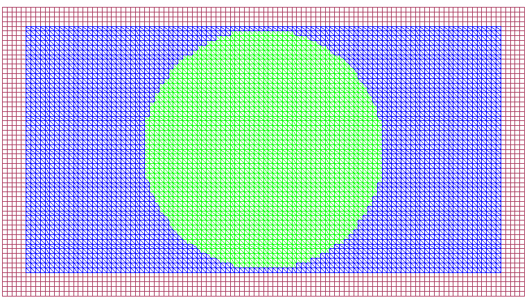
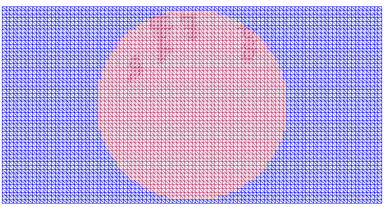
Refer to caption Refer to captionΩ2subscriptΩ2\Omega_{2}Ω1subscriptΩ1\Omega_{1}
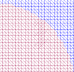
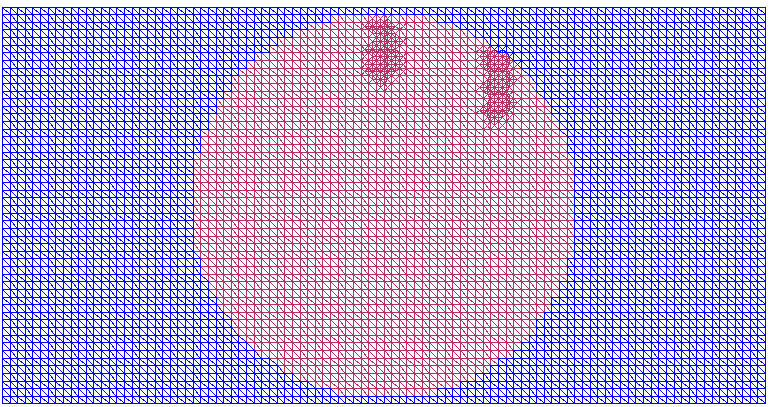
a) ΩΩ\Omega b) ΩFEM=Ω1Ω2subscriptΩ𝐹𝐸𝑀subscriptΩ1subscriptΩ2\Omega_{FEM}=\Omega_{1}\cup\Omega_{2}
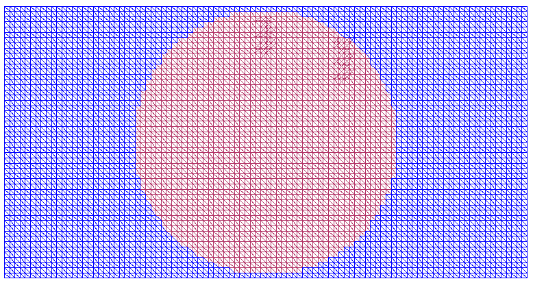
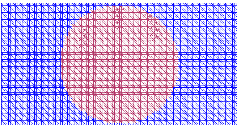
Figure 1: a) Computational mesh used in the domain decomposition of the domain Ω=ΩFEMΩFDMΩsubscriptΩ𝐹𝐸𝑀subscriptΩ𝐹𝐷𝑀\Omega=\Omega_{FEM}\cup\Omega_{FDM}. b) The finite element mesh in ΩFEM=Ω1Ω2subscriptΩ𝐹𝐸𝑀subscriptΩ1subscriptΩ2\Omega_{FEM}=\Omega_{1}\cup\Omega_{2}.
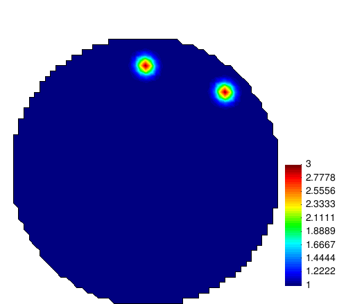
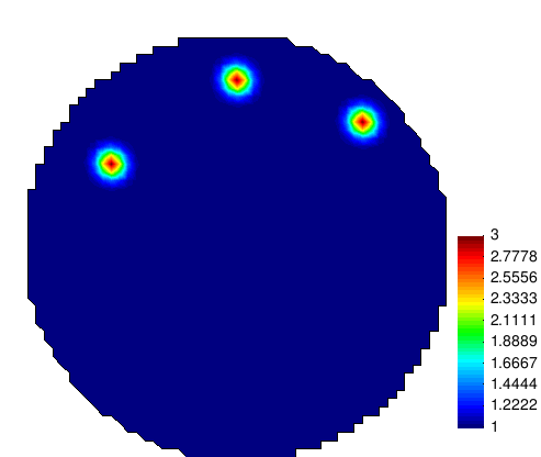
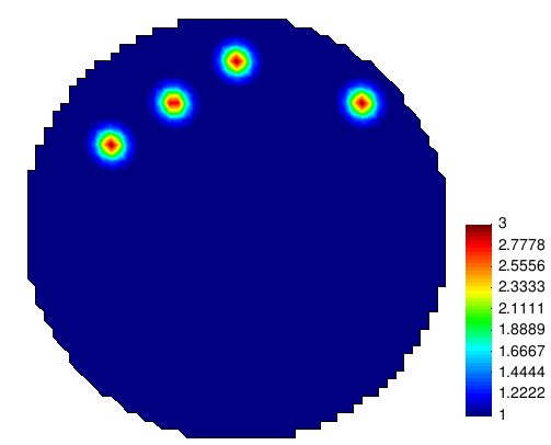
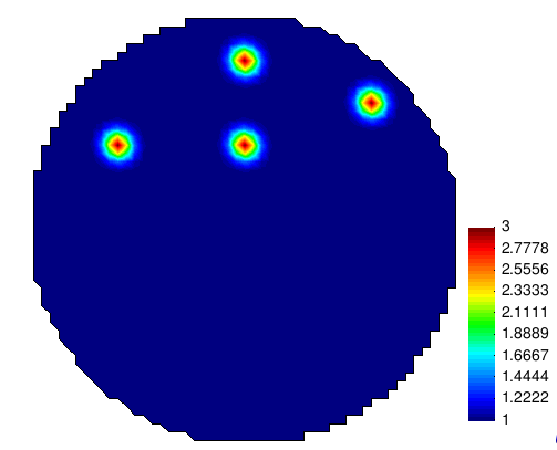
Exact ρ(x)𝜌𝑥\rho(x)
Test 1 Test 2 Test 3 Test 4
Refer to caption Refer to caption Refer to caption Refer to caption
Exact p(x)𝑝𝑥p(x)
Test 1 Test 2 Test 3 Test 4
Refer to caption Refer to caption Refer to caption Refer to caption
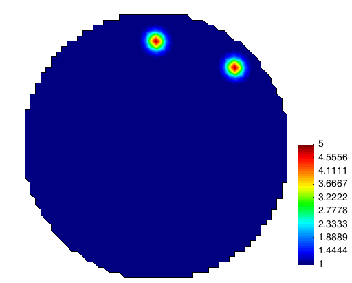
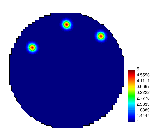
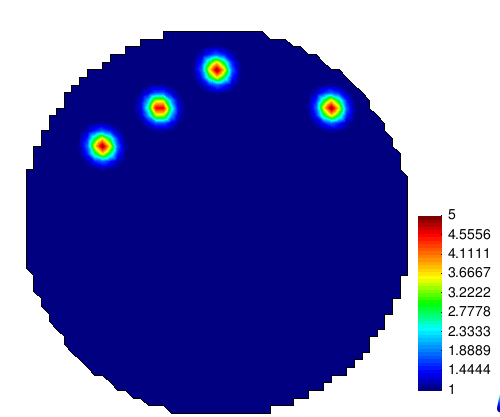
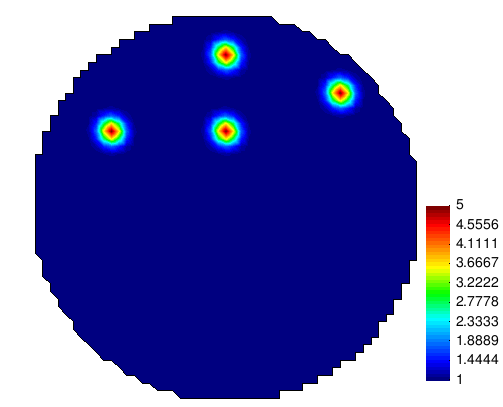
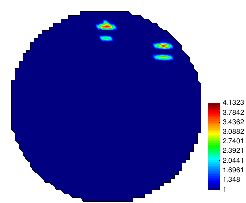
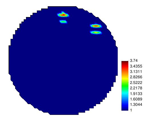
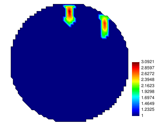
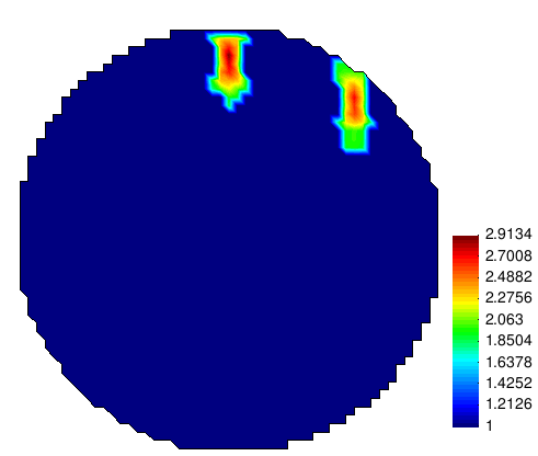
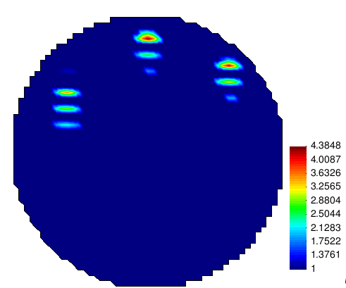
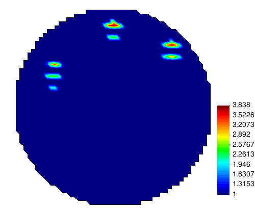
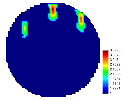
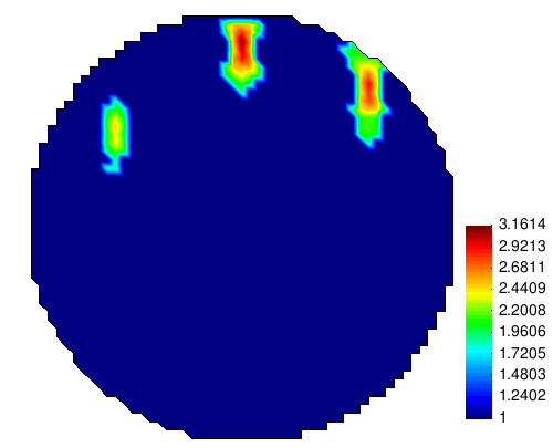
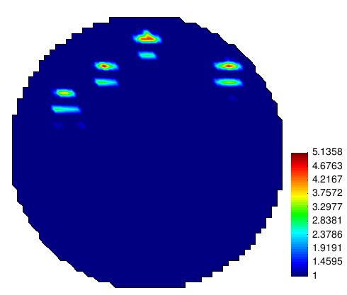
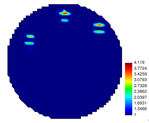
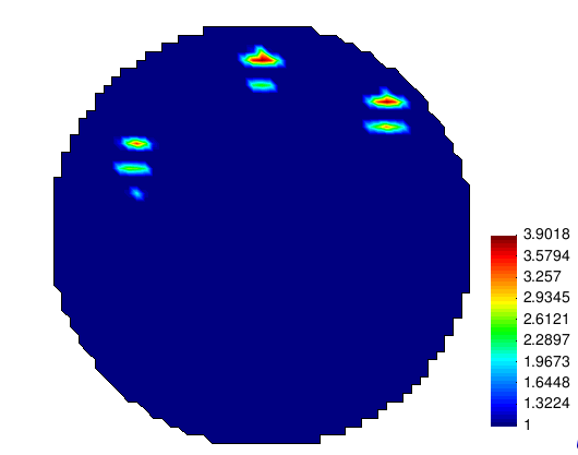
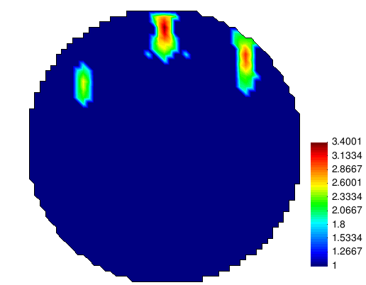
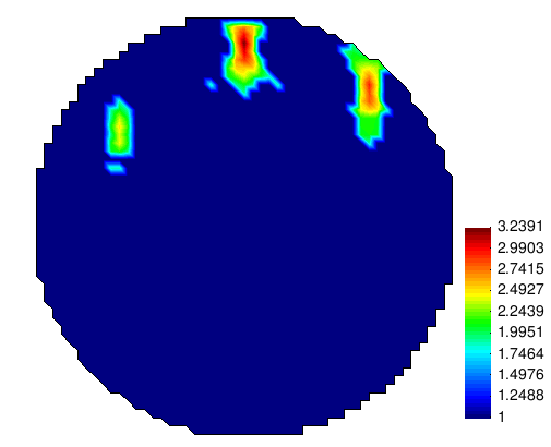
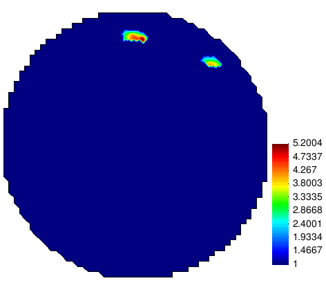
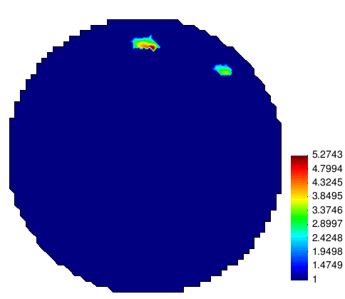
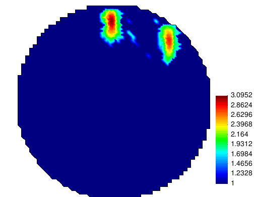
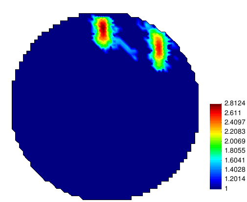
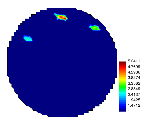
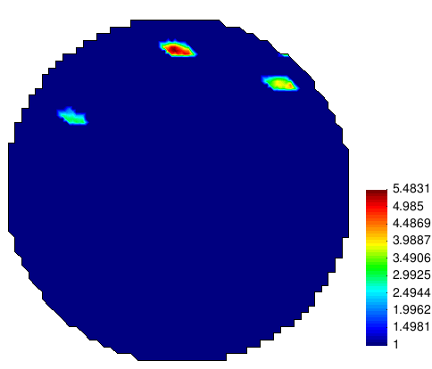
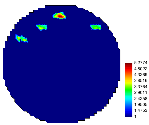
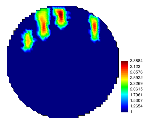
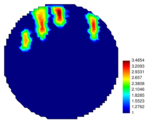
Figure 2: Exact Gaussian functions ρ(x)𝜌𝑥\rho(x) and p(x)𝑝𝑥p(x) in Ω1subscriptΩ1\Omega_{1} in different tests.
Test 1
ρ(x),δ=3%𝜌𝑥𝛿percent3\rho(x),\delta=3\% ρ(x),δ=10%𝜌𝑥𝛿percent10\rho(x),\delta=10\% p(x),δ=3%𝑝𝑥𝛿percent3p(x),\delta=3\% p(x),δ=10%𝑝𝑥𝛿percent10p(x),\delta=10\%
Refer to caption Refer to caption Refer to caption Refer to caption
Test 2
Refer to caption Refer to caption Refer to caption Refer to caption
Test 3
Refer to caption Refer to caption Refer to caption Refer to caption
Test 4
Refer to caption Refer to caption Refer to caption Refer to caption
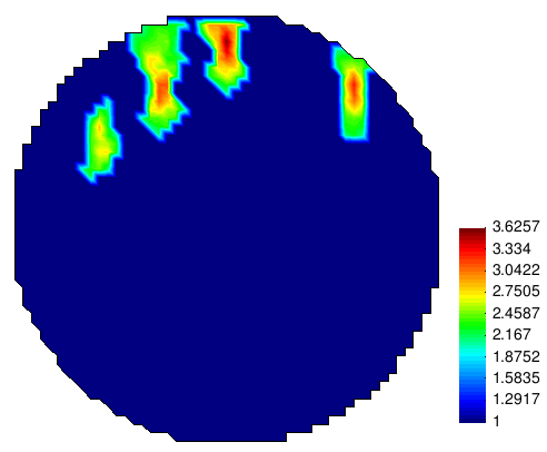
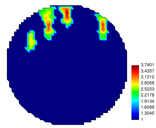
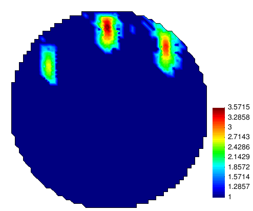
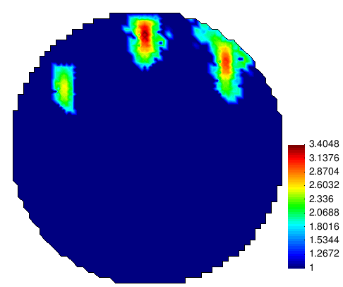
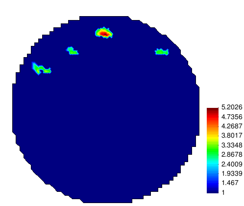
Figure 3: Reconstructions obtained in Tests 1-4 on a coarse mesh for different noise levels δ𝛿\delta in data.

4 Numerical Studies

In this section, we present numerical simulations of the reconstruction of two unknown functions ρ(x)𝜌𝑥\rho(x) and p(x)𝑝𝑥p(x) of the equation (1.1) using the domain decomposition method of [3].

To do that we decompose the computational domain ΩΩ\Omega into two subregions ΩFEMsubscriptΩ𝐹𝐸𝑀\Omega_{FEM} and ΩFDMsubscriptΩ𝐹𝐷𝑀\Omega_{FDM} such that Ω=ΩFEMΩFDMΩsubscriptΩ𝐹𝐸𝑀subscriptΩ𝐹𝐷𝑀\Omega=\Omega_{FEM}\cup\Omega_{FDM} with two layers of structured overlapping nodes between these domains, see Figure 1 and Figure 2 of [4] for details about communication between ΩFEMsubscriptΩ𝐹𝐸𝑀\Omega_{FEM} and ΩFDMsubscriptΩ𝐹𝐷𝑀\Omega_{FDM}. We will apply in our computations the finite element method (FEM) in ΩFEMsubscriptΩ𝐹𝐸𝑀\Omega_{FEM} and the finite difference method (FDM) in ΩFDMsubscriptΩ𝐹𝐷𝑀\Omega_{FDM}. We also decompose the domain ΩFEMsubscriptΩ𝐹𝐸𝑀\Omega_{FEM} into two different domains Ω1,Ω2subscriptΩ1subscriptΩ2\Omega_{1},\Omega_{2} such that ΩFEM=Ω1Ω2subscriptΩ𝐹𝐸𝑀subscriptΩ1subscriptΩ2\Omega_{FEM}=\Omega_{1}\cup\Omega_{2} which are intersecting only by their boundaries, see Figure 1. We use the domain decomposition approach in our computations since it is efficiently implemented in the high performance software package WavES [47] using C++ and PETSc [45]. For further details about construction of ΩFDMsubscriptΩ𝐹𝐷𝑀\Omega_{FDM} and ΩFEMsubscriptΩ𝐹𝐸𝑀\Omega_{FEM} domains as well as the domain decomposition method we refer to [3].

The boundary ΩΩ\partial\Omega of the domain ΩΩ\Omega is such that Ω=1Ω2Ω3ΩΩsubscript1Ωsubscript2Ωsubscript3Ω\partial\Omega=\partial_{1}\Omega\cup\partial_{2}\Omega\cup\partial_{3}\Omega where 1Ωsubscript1Ω\partial_{1}\Omega and 2Ωsubscript2Ω\partial_{2}\Omega are, respectively, top and bottom parts of ΩΩ\Omega, and 3Ωsubscript3Ω\partial_{3}\Omega is the union of left and right sides of this domain. We will collect time-dependent observations Γ1:=1Ω×(0,T)assignsubscriptΓ1subscript1Ω0𝑇\Gamma_{1}:=\partial_{1}\Omega\times(0,T) at the backscattering side 1Ωsubscript1Ω\partial_{1}\Omega of ΩΩ\Omega. We also define Γ1,1:=1Ω×(0,t1]assignsubscriptΓ11subscript1Ω0subscript𝑡1\Gamma_{1,1}:=\partial_{1}\Omega\times(0,t_{1}], Γ1,2:=1Ω×(t1,T)assignsubscriptΓ12subscript1Ωsubscript𝑡1𝑇\Gamma_{1,2}:=\partial_{1}\Omega\times(t_{1},T), Γ2:=2Ω×(0,T)assignsubscriptΓ2subscript2Ω0𝑇\Gamma_{2}:=\partial_{2}\Omega\times(0,T) and Γ3:=3Ω×(0,T)assignsubscriptΓ3subscript3Ω0𝑇\Gamma_{3}:=\partial_{3}\Omega\times(0,T).

We have used the following model problem in all computations:

ρ(x)t2u(x,t)div((p(x)u(x,t))=0inΩT,u(x,0)=a(x),ut(x,0)=0inΩ,nu=f(t)onΓ1,1,nu=tuonΓ1,2,nu=tuonΓ2,nu=0onΓ3.\begin{split}\rho(x)\partial_{t}^{2}u(x,t)-\mbox{div}\thinspace((p(x)\nabla u(x,t))&=0~{}\mbox{in}~{}~{}\Omega_{T},\\ u(x,0)=a(x),~{}~{}~{}u_{t}(x,0)&=0~{}\mbox{in}~{}~{}\Omega,\\ \partial_{n}u&=f(t)~{}\mbox{on}~{}\Gamma_{1,1},\\ \partial_{n}u&=-\partial_{t}u~{}\mbox{on}~{}\Gamma_{1,2},\\ \partial_{n}u&=-\partial_{t}u~{}\mbox{on}~{}\Gamma_{2},\\ \partial_{n}u&=0~{}\mbox{on}~{}\Gamma_{3}.\\ \end{split} (4.1)

In (4.1) the function f(t)𝑓𝑡f(t) represents the single direction of a plane wave which is initialized at 1Ωsubscript1Ω\partial_{1}\Omega in time t=[0,2.0]𝑡02.0t=[0,2.0] and is defined as

f(t)={sin(ωft), if t(0,2πωf),0, if t>2πωf.𝑓𝑡casessubscript𝜔𝑓𝑡 if 𝑡02𝜋subscript𝜔𝑓0 if 𝑡2𝜋subscript𝜔𝑓\begin{split}f(t)=\left\{\begin{array}[]{ll}\sin\left(\omega_{f}t\right),&\text{ if }t\in\left(0,\frac{2\pi}{\omega_{f}}\right),\\ 0,&\text{ if }t>\frac{2\pi}{\omega_{f}}.\end{array}\right.\end{split} (4.2)

We initialize initial condition a(x)𝑎𝑥a(x) at the boundary 1Ωsubscript1Ω\partial_{1}\Omega as

u(x,0)=f0(x)=e(x12+x22+x33)cost|t=0=e(x12+x22+x33).𝑢𝑥0subscript𝑓0𝑥evaluated-atsuperscriptesuperscriptsubscript𝑥12superscriptsubscript𝑥22superscriptsubscript𝑥33𝑡𝑡0superscriptesuperscriptsubscript𝑥12superscriptsubscript𝑥22superscriptsubscript𝑥33\begin{split}u(x,0)&=f_{0}(x)={\rm e}^{-(x_{1}^{2}+x_{2}^{2}+x_{3}^{3})}\cdot\cos t|_{t=0}={\rm e}^{-(x_{1}^{2}+x_{2}^{2}+x_{3}^{3})}.\end{split} (4.3)

We assume that both functions ρ(x)=p(x)=1𝜌𝑥𝑝𝑥1\rho(x)=p(x)=1 are known inside ΩFDMΩ2subscriptΩ𝐹𝐷𝑀subscriptΩ2\Omega_{FDM}\cup\Omega_{2}. The goal of our numerical tests is to reconstruct simultaneously two smooth functions ρ(x),p(x)𝜌𝑥𝑝𝑥\rho(x),p(x) of the domain Ω1subscriptΩ1\Omega_{1} of Figure 1. The main feature of these functions is that they model inclusions of a very small sizes what can be of practical interest in real-life applications.

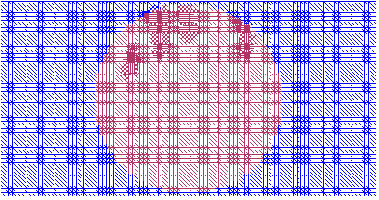
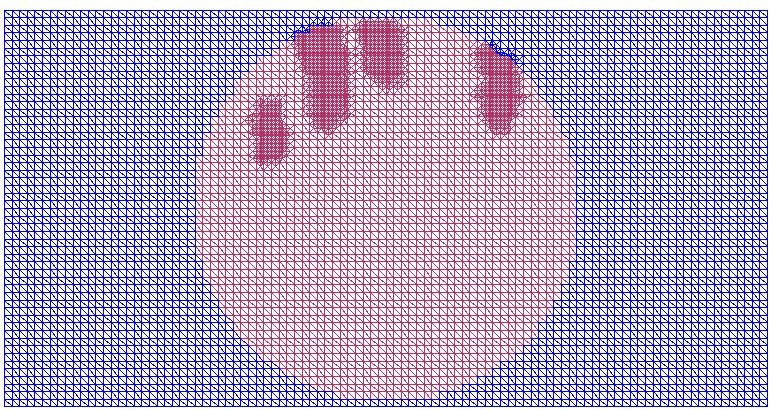
adaptively refined meshes zoomed
Refer to caption Refer to caption
once refined mesh
Refer to caption Refer to caption
twice refined mesh
Refer to caption Refer to caption
three times refined mesh
ρ(x),δ=3%𝜌𝑥𝛿percent3\rho(x),\delta=3\% ρ(x),δ=10%𝜌𝑥𝛿percent10\rho(x),\delta=10\% p(x),δ=3%𝑝𝑥𝛿percent3p(x),\delta=3\% p(x),δ=10%𝑝𝑥𝛿percent10p(x),\delta=10\%
Refer to caption Refer to caption Refer to caption Refer to caption
Figure 4: Test 1: reconstructions obtained on three times adaptively refined mesh for different noise levels δ𝛿\delta in data.
adaptively refined meshes zoomed
Refer to caption Refer to caption
once refined mesh
Refer to caption Refer to caption
twice refined mesh
Refer to caption Refer to caption
three times refined mesh
ρ(x),δ=3%𝜌𝑥𝛿percent3\rho(x),\delta=3\% ρ(x),δ=10%𝜌𝑥𝛿percent10\rho(x),\delta=10\% p(x),δ=3%𝑝𝑥𝛿percent3p(x),\delta=3\% p(x),δ=10%𝑝𝑥𝛿percent10p(x),\delta=10\%
Refer to caption Refer to caption Refer to caption Refer to caption
Figure 5: Test 2: reconstructions obtained on two times adaptively refined mesh for different noise levels δ𝛿\delta in data.
adaptively refined meshes zoomed
Refer to caption Refer to caption
once refined mesh
Refer to caption Refer to caption
twice refined mesh
Refer to caption Refer to caption
three times refined mesh
ρ(x),δ=3%𝜌𝑥𝛿percent3\rho(x),\delta=3\% ρ(x),δ=10%𝜌𝑥𝛿percent10\rho(x),\delta=10\% p(x),δ=3%𝑝𝑥𝛿percent3p(x),\delta=3\% p(x),δ=10%𝑝𝑥𝛿percent10p(x),\delta=10\%
Refer to caption Refer to caption Refer to caption Refer to caption
Figure 6: Test 3: reconstructions obtained on three times adaptively refined mesh for different noise levels δ𝛿\delta in data.

We set the dimensionless computational domain ΩΩ\Omega in the domain decomposition as

Ω={x=(x1,x2):x1(1.1,1.1),x2(0.62,0.62)},Ωconditional-set𝑥subscript𝑥1subscript𝑥2formulae-sequencesubscript𝑥11.11.1subscript𝑥20.620.62\Omega=\left\{x=(x_{1},x_{2}):x_{1}\in(-1.1,1.1),x_{2}\in(-0.62,0.62)\right\},

and the domain ΩFEMsubscriptΩ𝐹𝐸𝑀\Omega_{FEM} as

ΩFEM={x=(x1,x2):x1(1.0,1.0),x2(0.52,0.52)}.subscriptΩ𝐹𝐸𝑀conditional-set𝑥subscript𝑥1subscript𝑥2formulae-sequencesubscript𝑥11.01.0subscript𝑥20.520.52\Omega_{FEM}=\left\{x=(x_{1},x_{2}):x_{1}\in(-1.0,1.0),x_{2}\in(-0.52,0.52)\right\}.

We choose the mesh size h=0.020.02h=0.02 in Ω=ΩFEMΩFDMΩsubscriptΩ𝐹𝐸𝑀subscriptΩ𝐹𝐷𝑀\Omega=\Omega_{FEM}\cup\Omega_{FDM}, as well as in the overlapping regions between FE/FD domains.

We assume that our two functions ρ(x),p(x)𝜌𝑥𝑝𝑥\rho(x),p(x) belongs to the set of admissible parameters

Mρ={ρC2(Ω¯);1ρ(x)10},Mp={pC2(Ω¯);1p(x)5}.formulae-sequencesubscript𝑀𝜌formulae-sequence𝜌superscript𝐶2¯Ω1𝜌𝑥10subscript𝑀𝑝formulae-sequence𝑝superscript𝐶2¯Ω1𝑝𝑥5\begin{split}M_{\rho}&=\{\rho\in C^{2}(\overline{\Omega});~{}1\leq\rho(x)\leq 10\},\\ M_{p}&=\{p\in C^{2}(\overline{\Omega});~{}1\leq p(x)\leq 5\}.\end{split} (4.4)

We define now our coefficient inverse problem which we use in computations.

Inverse Problem (IP) Assume that the functions ρ(x),p(x)𝜌𝑥𝑝𝑥\rho(x),p(x)  of the model problem (4.1) are unknown. Let these functions satisfy conditions (4.4,) and ρ(x)=1,p(x)=1formulae-sequence𝜌𝑥1𝑝𝑥1\rho(x)=1,p(x)=1 in the domain Ω\ΩFEM\ΩsubscriptΩFEM\Omega\backslash\Omega_{\rm FEM}. Determine the functions ρ(x),p(x)𝜌𝑥𝑝𝑥\rho(x),p(x) for xΩ\ΩFDM,𝑥\ΩsubscriptΩFDMx\in\Omega\backslash\Omega_{\rm FDM},  assuming that the following function u~(x,t)~𝑢𝑥𝑡\tilde{u}\left(x,t\right) is known

u(x,t)=u~(x,t),(x,t)Γ1.formulae-sequence𝑢𝑥𝑡~𝑢𝑥𝑡for-all𝑥𝑡subscriptΓ1u\left(x,t\right)=\tilde{u}\left(x,t\right),\forall\left(x,t\right)\in\Gamma_{1}. (4.5)

To determine both coefficients ρ(x),p(x)𝜌𝑥𝑝𝑥\rho(x),p(x) in inverse problem IP we minimize the following Tikhonov functional

J(ρ(x),p(x)):=J(u,ρ,p)=12Γ1(uu~)2zδ(t)𝑑s𝑑t+12α1Ω(ρρ0)2𝑑x+12α2Ω(pp0)2𝑑x.assign𝐽𝜌𝑥𝑝𝑥𝐽𝑢𝜌𝑝12subscriptsubscriptΓ1superscript𝑢~𝑢2subscript𝑧𝛿𝑡differential-d𝑠differential-d𝑡12subscript𝛼1subscriptΩsuperscript𝜌subscript𝜌02differential-d𝑥12subscript𝛼2subscriptΩsuperscript𝑝subscript𝑝02differential-d𝑥\begin{split}J(\rho(x),p(x))&:=J(u,\rho,p)=\frac{1}{2}\int_{\Gamma_{1}}(u-\tilde{u})^{2}z_{\delta}(t)dsdt\\ &+\frac{1}{2}\alpha_{1}\int_{\Omega}(\rho-\rho_{0})^{2}~{}~{}dx+\frac{1}{2}\alpha_{2}\int_{\Omega}(p-p_{0})^{2}~{}~{}dx.\end{split} (4.6)

Here, u~~𝑢\tilde{u} is the observed function u𝑢u in time at the backscattered boundary 1Ωsubscript1Ω\partial_{1}\Omega, the function u𝑢u satisfy the equations (4.1) and thus depends on ρ,p𝜌𝑝\rho,p, ρ0,p0subscript𝜌0subscript𝑝0\rho_{0},p_{0} are the initial guesses for ρ,p𝜌𝑝\rho,p, correspondingly, and αi,i=1,2formulae-sequencesubscript𝛼𝑖𝑖12\alpha_{i},i=1,2, are regularization parameters. We take ρ0=1,p0=1formulae-sequencesubscript𝜌01subscript𝑝01\rho_{0}=1,p_{0}=1 at all points of the computational domain since previous computational works [3, 10, 2, 7] as well as experimental works of [43, 44] have shown that a such choice gives good results of reconstruction. Here, zδ(t)subscript𝑧𝛿𝑡z_{\delta}(t) is a cut-off function chosen as in [3, 10, 7]. This function is introduced to ensure the compatibility conditions at Ω¯T{t=T}subscript¯Ω𝑇𝑡𝑇\overline{\Omega}_{T}\cap\left\{t=T\right\} for the adjoint problem, see details in [3, 10, 7].

To solve the minimization problem we take into account conditions (4.4) and introduce the Lagrangian

L(v)=J(u,ρ,p)+Ω0Tλ(ρ2ut2div(pu))𝑑x𝑑t,𝐿𝑣𝐽𝑢𝜌𝑝subscriptΩsuperscriptsubscript0𝑇𝜆𝜌superscript2𝑢superscript𝑡2div𝑝𝑢differential-d𝑥differential-d𝑡\begin{split}L(v)&=J(u,\rho,p)+\int_{\Omega}\int_{0}^{T}\lambda\Big{(}\rho\frac{\partial^{2}u}{\partial t^{2}}-\mbox{div}\thinspace(p\nabla u)\Big{)}~{}dxdt,\end{split} (4.7)

where v=(u,λ,ρ,p)𝑣𝑢𝜆𝜌𝑝v=(u,\lambda,\rho,p). Our goal is to find a stationary point of the Lagrangian with respect to v𝑣v satisfying v¯=(u¯,λ¯,ρ¯,p¯)for-all¯𝑣¯𝑢¯𝜆¯𝜌¯𝑝\forall\bar{v}=(\bar{u},\bar{\lambda},\bar{\rho},\bar{p})

L(v;v¯)=0,superscript𝐿𝑣¯𝑣0L^{\prime}(v;\bar{v})=0, (4.8)

where L(v;)superscript𝐿𝑣L^{\prime}(v;\cdot) is the Jacobian of L𝐿L at v𝑣v. To find optimal parameters ρ,p𝜌𝑝\rho,p from (4.8) we use the conjugate gradient method with iterative choice of the regularization parameters αj,j=1,2formulae-sequencesubscript𝛼𝑗𝑗12\alpha_{j},j=1,2, in (4.6). More precisely, in all our computations we choose the regularization parameters iteratively as was proposed in [1], such that αjn=αj0(n+1)qsubscriptsuperscript𝛼𝑛𝑗subscriptsuperscript𝛼0𝑗superscript𝑛1𝑞\alpha^{n}_{j}=\alpha^{0}_{j}(n+1)^{-q}, where n𝑛n is the number of iteration in the conjugate gradient method, q(0,1)𝑞01q\in(0,1) and αj0subscriptsuperscript𝛼0𝑗\alpha^{0}_{j} are initial guesses for αj,j=1,2formulae-sequencesubscript𝛼𝑗𝑗12\alpha_{j},j=1,2. Similarly with [35] we take αj=δζsubscript𝛼𝑗superscript𝛿𝜁\alpha_{j}=\delta^{\zeta}, where δ𝛿\delta is the noise level and ζ𝜁\zeta is a small number taken in the interval (0,1)01(0,1). Different techniques for the computation of a regularization parameter are presented in works [23, 30, 31, 46], and checking of performance of these techniques for the solution of our inverse problem can be challenge for our future research.

To generate backscattered data we solve the model problem (4.1) in time T=[0,2.0]𝑇02.0T=[0,2.0] with the time step τ=0.002𝜏0.002\tau=0.002 which satisfies to the CFL condition [21]. In order to check performance of the reconstruction algorithm we supply simulated backscattered data at 1Ωsubscript1Ω\partial_{1}\Omega by additive, as in [3, 10, 7], noise δ=3%,10%𝛿percent3percent10\delta=3\%,10\%. Similar results of reconstruction are obtained for random noise and they will be presented in the forthcoming publication.

Table 1. Computational results of the reconstructions on a coarse and on adaptively refined meshes together with computational errors in the maximal contrast of ρ(x),p(x)𝜌𝑥𝑝𝑥\rho(x),p(x) in percents. Here, Nρj,Npjsuperscriptsubscript𝑁𝜌𝑗superscriptsubscript𝑁𝑝𝑗N_{\rho}^{j},N_{p}^{j} denote the final number of iterations in the conjugate gradient method on j𝑗j times refined mesh for reconstructed functions ρ𝜌\rho and p𝑝p, respectively.

Coarse mesh δ=3%𝛿percent3\delta=3\% δ=10%𝛿percent10\delta=10\% Case maxΩ1ρsubscriptsubscriptΩ1𝜌\max_{\Omega_{1}}\rho error, % Nρ0superscriptsubscript𝑁𝜌0N_{\rho}^{0} Test 1 4.13 17.4 13 Test 2 4.38 12.4 151515 Test 3 5.14 2.8 161616 Test 4 4.12 17.6 141414 Case maxΩ1ρsubscriptsubscriptΩ1𝜌\max_{\Omega_{1}}\rho error, % Nρ0superscriptsubscript𝑁𝜌0N_{\rho}^{0} Test 1 3.74 25.2 12 Test 2 3.84 23.2 131313 Test 3 5.08 1.6 161616 Test 4 3.9 22 131313 Case maxΩ1psubscriptsubscriptΩ1𝑝\max_{\Omega_{1}}p error, % Np0superscriptsubscript𝑁𝑝0N_{p}^{0} Test 1 3.09 3 131313 Test 2 3.63 21 151515 Test 3 3.63 21 161616 Test 4 3.4 13.3 141414 Case maxΩ1psubscriptsubscriptΩ1𝑝\max_{\Omega_{1}}p error, % Np0superscriptsubscript𝑁𝑝0N_{p}^{0} Test 1 2.9 3.33 121212 Test 2 3.16 5.33 131313 Test 3 3.74 24.67 161616 Test 4 3.24 8 13 Adaptively refined mesh Case maxΩ1ρsubscriptsubscriptΩ1𝜌\max_{\Omega_{1}}\rho error, % Nρjsuperscriptsubscript𝑁𝜌𝑗N_{\rho}^{j} Test 1 5.2 4 Nρ3=9superscriptsubscript𝑁𝜌39N_{\rho}^{3}=9 Test 2 5.24 4.8 Nρ2=6superscriptsubscript𝑁𝜌26N_{\rho}^{2}=6 Test 3 5.2 4 Nρ3=1superscriptsubscript𝑁𝜌31N_{\rho}^{3}=1 Test 4 5.5 10 Nρ3=8superscriptsubscript𝑁𝜌38N_{\rho}^{3}=8 Case maxΩ1ρsubscriptsubscriptΩ1𝜌\max_{\Omega_{1}}\rho error, % Nρjsuperscriptsubscript𝑁𝜌𝑗N_{\rho}^{j} Test 1 5.3 6 Nρ3=7superscriptsubscript𝑁𝜌37N_{\rho}^{3}=7 Test 2 5.5 10 Nρ2=10superscriptsubscript𝑁𝜌210N_{\rho}^{2}=10 Test 3 5.28 5.6 Nρ3=1superscriptsubscript𝑁𝜌31N_{\rho}^{3}=1 Test 4 5.36 7.2 Nρ3=8superscriptsubscript𝑁𝜌38N_{\rho}^{3}=8 Case maxΩ1psubscriptsubscriptΩ1𝑝\max_{\Omega_{1}}p error, % Npjsuperscriptsubscript𝑁𝑝𝑗N_{p}^{j} Test 1 3.1 3.33 Np3=9superscriptsubscript𝑁𝑝39N_{p}^{3}=9 Test 2 3.57 19 Np2=6superscriptsubscript𝑁𝑝26N_{p}^{2}=6 Test 3 3.39 13 Np3=1superscriptsubscript𝑁𝑝31N_{p}^{3}=1 Test 4 3.4 13.3 Np3=14superscriptsubscript𝑁𝑝314N_{p}^{3}=14 Case maxΩ1psubscriptsubscriptΩ1𝑝\max_{\Omega_{1}}p error, % Npjsuperscriptsubscript𝑁𝑝𝑗N_{p}^{j} Test 1 2.8 6.67 Np3=7superscriptsubscript𝑁𝑝37N_{p}^{3}=7 Test 2 3.4 13.3 Np2=9superscriptsubscript𝑁𝑝29N_{p}^{2}=9 Test 3 3.49 16.3 Np3=1superscriptsubscript𝑁𝑝31N_{p}^{3}=1 Test 4 3.26 8.67 Np3=10superscriptsubscript𝑁𝑝310N_{p}^{3}=10

4.1 Test 1

In this test we present numerical results of the simultaneous reconstruction of two functions ρ(x)𝜌𝑥\rho(x) and p(x)𝑝𝑥p(x) given by

ρ(x)=1.0+4.0e((x10.3)2+(x20.3)2)/0.001+4.0e(x12+(x20.4)2)/0.001,p(x)=1.0+2.0e((x10.3)2+(x20.3)2)/0.001+2.0e(x12+(x20.4)2)/0.001,formulae-sequence𝜌𝑥1.04.0superscriptesuperscriptsubscript𝑥10.32superscriptsubscript𝑥20.320.0014.0superscriptesuperscriptsubscript𝑥12superscriptsubscript𝑥20.420.001𝑝𝑥1.02.0superscriptesuperscriptsubscript𝑥10.32superscriptsubscript𝑥20.320.0012.0superscriptesuperscriptsubscript𝑥12superscriptsubscript𝑥20.420.001\begin{split}\rho(x)=1.0&+4.0\cdot{\rm e}^{-((x_{1}-0.3)^{2}+{(x_{2}-0.3)}^{2})/0.001}\\ &+4.0\cdot{\rm e}^{-(x_{1}^{2}+{(x_{2}-0.4)}^{2})/0.001},\\ p(x)=1.0&+2.0\cdot{\rm e}^{-((x_{1}-0.3)^{2}+{(x_{2}-0.3)}^{2})/0.001}\\ &+2.0\cdot{\rm e}^{-(x_{1}^{2}+{(x_{2}-0.4)}^{2})/0.001},\\ \end{split} (4.9)

which are presented in Figure  2.

Figures 3 show results of the reconstruction on a coarse mesh with additive noise δ=3%,10%𝛿percent3percent10\delta=3\%,10\% in data. We observe that the location of both functions ρ,p𝜌𝑝\rho,p given by (4.9) is imaged correctly. We refer to Table 1 for the reconstruction of the contrast in both functions.

To improve contrast and shape of the reconstructed functions ρ(x)𝜌𝑥\rho(x) and p(x)𝑝𝑥p(x) we run computations again using an adaptive conjugate gradient method similar to the one of [7]. Figure 4 and Table 1 show results of reconstruction on the three times locally refined mesh. We observe that we achieve better contrast for both functions ρ(x)𝜌𝑥\rho(x) and p(x)𝑝𝑥p(x), as well as better shape for the function ρ(x)𝜌𝑥\rho(x).

4.2 Test 2

In this test we present numerical results of the reconstruction of the functions ρ(x)𝜌𝑥\rho(x) and p(x)𝑝𝑥p(x) given by three Gaussians shown in Figure  2 and given by

ρ(x)=1.0+4.0e((x10.3)2+(x20.3)2)/0.001+4.0e(x12+(x20.4)2)/0.001+4.0e((x1+0.3)2+(x20.2)2)/0.001,p(x)=1.0+2.0e((x10.3)2+(x20.3)2)/0.001+2.0e(x12+(x20.4)2)/0.001+2.0e((x1+0.3)2+(x20.2)2)/0.001.formulae-sequence𝜌𝑥1.04.0superscriptesuperscriptsubscript𝑥10.32superscriptsubscript𝑥20.320.0014.0superscriptesuperscriptsubscript𝑥12superscriptsubscript𝑥20.420.0014.0superscriptesuperscriptsubscript𝑥10.32superscriptsubscript𝑥20.220.001𝑝𝑥1.02.0superscriptesuperscriptsubscript𝑥10.32superscriptsubscript𝑥20.320.0012.0superscriptesuperscriptsubscript𝑥12superscriptsubscript𝑥20.420.0012.0superscriptesuperscriptsubscript𝑥10.32superscriptsubscript𝑥20.220.001\begin{split}\rho(x)=1.0&+4.0\cdot{\rm e}^{-((x_{1}-0.3)^{2}+{(x_{2}-0.3)}^{2})/0.001}\\ &+4.0\cdot{\rm e}^{-(x_{1}^{2}+{(x_{2}-0.4)}^{2})/0.001}\\ &+4.0\cdot{\rm e}^{-((x_{1}+0.3)^{2}+{(x_{2}-0.2)}^{2})/0.001},\\ p(x)=1.0&+2.0\cdot{\rm e}^{-((x_{1}-0.3)^{2}+{(x_{2}-0.3)}^{2})/0.001}\\ &+2.0\cdot{\rm e}^{-(x_{1}^{2}+{(x_{2}-0.4)}^{2})/0.001}\\ &+2.0\cdot{\rm e}^{-((x_{1}+0.3)^{2}+{(x_{2}-0.2)}^{2})/0.001}.\end{split} (4.10)

Figures 3 show results of the reconstruction on a coarse mesh with additive noise δ=3%,10%𝛿percent3percent10\delta=3\%,10\% in data. We observe that the location of three Gaussians for both functions ρ,p𝜌𝑝\rho,p is imaged correctly, see Table 1 for the reconstruction of contrast in these functions.

To improve contrast and shape of the reconstructed functions ρ(x)𝜌𝑥\rho(x) and p(x)𝑝𝑥p(x) we run computations again using an adaptive conjugate gradient method similar to the one of [7]. Figure 5 and Table 1 show results of reconstruction on the two times locally refined mesh. We observe that we achieve better contrast for both functions ρ(x)𝜌𝑥\rho(x) and p(x)𝑝𝑥p(x), as well as better shape for the function ρ(x)𝜌𝑥\rho(x). Results on the three times refined mesh were similar to the results obtained on a two times refined mesh, and we are not presenting them here.

4.3 Test 3

This test presents numerical results of the reconstruction of the functions ρ(x)𝜌𝑥\rho(x) and p(x)𝑝𝑥p(x) given by four different Gaussians shown in Figure  2 and given by

ρ(x)=1.0+4.0e((x10.3)2+(x20.3)2)/0.001+4.0e(x12+(x20.4)2)/0.001+4.0e((x1+0.3)2+(x20.2)2)/0.001+4.0e((x1+0.15)2+(x20.3)2)/0.001,p(x)=1.0+2.0e((x10.3)2+(x20.3)2)/0.001+2.0e(x12+(x20.4)2)/0.001+2.0e((x1+0.3)2+(x20.2)2)/0.001+2.0e((x1+0.15)2+(x20.3)2)/0.001.formulae-sequence𝜌𝑥1.04.0superscriptesuperscriptsubscript𝑥10.32superscriptsubscript𝑥20.320.0014.0superscriptesuperscriptsubscript𝑥12superscriptsubscript𝑥20.420.0014.0superscriptesuperscriptsubscript𝑥10.32superscriptsubscript𝑥20.220.0014.0superscriptesuperscriptsubscript𝑥10.152superscriptsubscript𝑥20.320.001𝑝𝑥1.02.0superscriptesuperscriptsubscript𝑥10.32superscriptsubscript𝑥20.320.0012.0superscriptesuperscriptsubscript𝑥12superscriptsubscript𝑥20.420.0012.0superscriptesuperscriptsubscript𝑥10.32superscriptsubscript𝑥20.220.0012.0superscriptesuperscriptsubscript𝑥10.152superscriptsubscript𝑥20.320.001\begin{split}\rho(x)=1.0&+4.0\cdot{\rm e}^{-((x_{1}-0.3)^{2}+{(x_{2}-0.3)}^{2})/0.001}\\ &+4.0\cdot{\rm e}^{-(x_{1}^{2}+{(x_{2}-0.4)}^{2})/0.001}\\ &+4.0\cdot{\rm e}^{-((x_{1}+0.3)^{2}+{(x_{2}-0.2)}^{2})/0.001}\\ &+4.0\cdot{\rm e}^{-((x_{1}+0.15)^{2}+{(x_{2}-0.3)}^{2})/0.001},\\ p(x)=1.0&+2.0\cdot{\rm e}^{-((x_{1}-0.3)^{2}+{(x_{2}-0.3)}^{2})/0.001}\\ &+2.0\cdot{\rm e}^{-(x_{1}^{2}+{(x_{2}-0.4)}^{2})/0.001}\\ &+2.0\cdot{\rm e}^{-((x_{1}+0.3)^{2}+{(x_{2}-0.2)}^{2})/0.001}\\ &+2.0\cdot{\rm e}^{-((x_{1}+0.15)^{2}+{(x_{2}-0.3)}^{2})/0.001}.\end{split} (4.11)

Figures 3 show results of the reconstruction of four Gaussians on a coarse mesh with additive noise δ=3%,10%𝛿percent3percent10\delta=3\%,10\% in data. We have obtained similar results as in the two previous tests: the location of four Gaussians for both functions ρ,p𝜌𝑝\rho,p already on a coarse mesh is imaged correctly. However, as follows from the Table 1, the contrast should be improved. Again, to improve the contrast and shape of the Gaussians we run an adaptive conjugate gradient method similar to one of [7]. Figure 6 shows results of reconstruction on the three times locally refined mesh. Using Table 1 we observe that we achieve better contrast for both functions ρ(x)𝜌𝑥\rho(x) and p(x)𝑝𝑥p(x), as well as better shape for the function ρ(x)𝜌𝑥\rho(x).

4.4 Test 4

In this test we tried to reconstruct four Gaussians shown in Figure  2 and given by

ρ(x)=1.0+4.0e((x10.3)2+(x20.3)2)/0.001+4.0e(x12+(x20.4)2)/0.001+4.0e((x1+0.3)2+(x20.2)2)/0.001+4.0e(x12+(x20.2)2)/0.001,p(x)=1.0+2.0e((x10.3)2+(x20.3)2)/0.001+2.0e(x12+(x20.4)2)/0.001+2.0e((x1+0.3)2+(x20.2)2)/0.001+2.0e(x12+(x20.2)2)/0.001.formulae-sequence𝜌𝑥1.04.0superscriptesuperscriptsubscript𝑥10.32superscriptsubscript𝑥20.320.0014.0superscriptesuperscriptsubscript𝑥12superscriptsubscript𝑥20.420.0014.0superscriptesuperscriptsubscript𝑥10.32superscriptsubscript𝑥20.220.0014.0superscriptesuperscriptsubscript𝑥12superscriptsubscript𝑥20.220.001𝑝𝑥1.02.0superscriptesuperscriptsubscript𝑥10.32superscriptsubscript𝑥20.320.0012.0superscriptesuperscriptsubscript𝑥12superscriptsubscript𝑥20.420.0012.0superscriptesuperscriptsubscript𝑥10.32superscriptsubscript𝑥20.220.0012.0superscriptesuperscriptsubscript𝑥12superscriptsubscript𝑥20.220.001\begin{split}\rho(x)=1.0&+4.0\cdot{\rm e}^{-((x_{1}-0.3)^{2}+{(x_{2}-0.3)}^{2})/0.001}\\ &+4.0\cdot{\rm e}^{-(x_{1}^{2}+{(x_{2}-0.4)}^{2})/0.001}\\ &+4.0\cdot{\rm e}^{-((x_{1}+0.3)^{2}+{(x_{2}-0.2)}^{2})/0.001}\\ &+4.0\cdot{\rm e}^{-(x_{1}^{2}+{(x_{2}-0.2)}^{2})/0.001},\\ p(x)=1.0&+2.0\cdot{\rm e}^{-((x_{1}-0.3)^{2}+{(x_{2}-0.3)}^{2})/0.001}\\ &+2.0\cdot{\rm e}^{-(x_{1}^{2}+{(x_{2}-0.4)}^{2})/0.001}\\ &+2.0\cdot{\rm e}^{-((x_{1}+0.3)^{2}+{(x_{2}-0.2)}^{2})/0.001}\\ &+2.0\cdot{\rm e}^{-(x_{1}^{2}+{(x_{2}-0.2)}^{2})/0.001}.\end{split} (4.12)

We observe that two Gaussians in this example are located one under another one. Thus, backscattered data from these two Gaussians will be superimposed and thus, we expect to reconstruct only three Gaussians from four.

Figure 3 shows results of the reconstruction of these four Gaussians on a coarse mesh with additive noise δ=3%,10%𝛿percent3percent10\delta=3\%,10\% in data. As expected, we could reconstruct only three Gaussians from four, see Table 1 for reconstruction of the contrast in them. Even application of the adaptive algorithm can not give us the fourth Gaussian. However, the contrast in the reconstructed functions is improved, as in Test 3.

5 Conclusions

In this work we present theoretical and numerical studies of the reconstruction of two space-dependent functions ρ(x)𝜌𝑥\rho(x) and p(x)𝑝𝑥p(x) in a hyperbolic problem.
In the theoretical part of this work we derive a local Carleman estimate which allows to obtain a conditional Lipschitz stability inequality for the inverse problem formulated in section 1. This stability is very important for our subsequent numerical reconstruction of the two unknown functions ρ(x)𝜌𝑥\rho(x) and p(x)𝑝𝑥p(x) in the hyperbolic model (4.1).
In the numerical part we present a computational study of the simultaneous reconstruction of two functions ρ(x)𝜌𝑥\rho(x) and p(x)𝑝𝑥p(x) in a hyperbolic problem (4.1) from backscattered data using an adaptive domain decomposition finite element/difference method similar to one developed in [3, 7]. In our numerical tests, we have obtained stable reconstruction of the location and contrasts of both functions ρ(x)𝜌𝑥\rho(x) and p(x)𝑝𝑥p(x) for noise levels δ=3%,10%𝛿percent3percent10\delta=3\%,10\% in backscattered data. Using results of Table 1 and Figures 46 we can conclude, that an adaptive domain decomposition finite element/finite difference algorithm significantly improves qualitative and quantitative results of the reconstruction obtained on a coarse mesh.

Acknowledgments

The research of L. B. is partially supported by the sabbatical programme at the Faculty of Science, University of Gothenburg, Sweden. The research of M.C. is partially supported by the guest programme of the Department of Mathematical Sciences at Chalmers University of Technology and Gothenburg University, Sweden. Research of M.Y. is partially supported by Grant-in-Aid for Scientific Research (S) 15H05740 of Japan Society for the Promotion of Science.

References

  • [1] A. Bakushinsky, M. Y. Kokurin, and A. Smirnova, Iterative Methods for Ill-posed Problems, De Gruyter, Berlin, 2011.
  • [2] L.Beilina, Adaptive Finite Element Method for a coefficient inverse problem for the Maxwell’s system, Applicable Analysis, 90 (2011), 1461–1479.
  • [3] L. Beilina, Domain Decomposition finite element/finite difference method for the conductivity reconstruction in a hyperbolic equation, Communications in Nonlinear Science and Numerical Simulation, Elsevier, 2016, doi:10.1016/j.cnsns.2016.01.016
  • [4] L. Beilina, Adaptive hybrid FEM/FDM methods for inverse scattering problems, Inverse Problems and Information Technologies, 1(3), 73–116, 2002.
  • [5] L. Beilina, M. Cristofol, and S. Li, Uniqueness and stability of time and space-dependent conductivity in a hyperbolic cylindrical domain, arXiv:1607.01615.
  • [6] L. Beilina, M. Cristofol, and K. Niinimäki, Optimization approach for the simultaneous reconstruction of the dielectric permittivity and magnetic permeability functions from limited observations, Inverse Problems and Imaging, 9 (2015), 1-25.
  • [7] L. Beilina and S. Hosseinzadegan, An adaptive finite element method in reconstruction of coefficients in Maxwell’s equations from limited observations, Applications of Mathematics, 61(3) (2016), 253–286.
  • [8] L. Beilina and C. Johnson, A posteriori error estimation in computational inverse scattering, Mathematical Models in Applied Sciences, 1 (2005), 23-35.
  • [9] L. Beilina and M.V. Klibanov, Approximate Global Convergence and Adaptivity for Coefficient Inverse Problems, Springer-Verlag, Berlin, 2012.
  • [10] L. Beilina and K. Niinimäki, Numerical studies of the Lagrangian approach for reconstruction of the conductivity in a waveguide, arXiv:1510.00499, 2015.
  • [11] M. Bellassoued, Uniqueness and stability in determining the speed of propagation of second order hyperbolic equation with variable coefficients, Appl. Anal. 83 (2004), 983-1014.
  • [12] M.Bellassoued, Global logarithmic stability in inverse hyperbolic problem by arbitrary boundary observation, Inverse Problems 20 (2004), 1033-1052.
  • [13] M. Bellassoued, M. Cristofol, and E. Soccorsi, Inverse boundary value problem for the dynamical heterogeneous Maxwell’s system, Inverse Problems 28 (2012), 095009.
  • [14] M. Bellassoued, O. Y. Imanuvilov, and M. Yamamoto, Inverse problem of determining the density and two Lame coefficients by boundary data, SIAM J. Math. Anal. 40 (2008), 238-265.
  • [15] M. Bellassoued, D. Jellali and M. Yamamoto, Lipschitz stability in in an inverse problem for a hyperbolic equation with a finite set of boundary data, Applicable Analysis 87 (2008), 1105-1119.
  • [16] M. Bellassoued and M. Yamamoto, Logarithmic stability in determination of a coefficient in an acoustic equation by arbitrary boundary observation, J. Math. Pures Appl. 85 (2006), 193-224.
  • [17] M. Bellassoued and M. Yamamoto, Determination of a coefficient in the wave equation with a single measurement, Appl. Anal. 87 (2008), 901-920.
  • [18] M. Bellassoued and M. Yamamoto, Carleman Estimates and Applications to Inverse Problems for Hyperbolic Systems, Springer-Japan, to appear.
  • [19] A.L. Bugkheim and M.V.Klibanov, Global uniqueness of class of multidimentional inverse problems, Soviet Math. Dokl. 24 (1981), 244-247.
  • [20] J. Cheng, V. Isakov, M. Yamamoto, and Q. Zhou, Lipschitz stability in the lateral Cauchy problem for elasticity system, J. Math. Kyoto Univ. 43 (2003), 475-501.
  • [21] R. Courant, K. Friedrichs and H. Lewy, On the partial differential equations of mathematical physics, Journal of Research and Development, 11(2) (1967), 215–234.
  • [22] Y. T. Chow and J. Zou, A numerical method for reconstructing the coefficient in a wave equation, Numerical Methods for Partial Differential Equations 31 (2015), 289–307.
  • [23] H. W. Engl, M. Hanke and A. Neubauer, Regularization of Inverse Problems, Kluwer, Boston, 2000.
  • [24] O. Y. Imanuvilov, On Carleman estimates for hyperbolic equations, Asymptotic Analysis 32 (2002), 185-220.
  • [25] O. Y. Imanuvilov, V. Isakov and M. Yamamoto, An inverse problem for the dynamical Lamé system with two sets of boundary data, Comm. Pure Appl. Math. 56 (2003), 1366-1382.
  • [26] O. Y. Imanuvilov and M. Yamamoto, Global uniqueness and stability in determining coefficients of wave equations, Comm. Partial Differential Equations 26 (2001), 1409-1425.
  • [27] O. Y. Imanuvilov and M. Yamamoto, Global Lipschitz stability in an inverse hyperbolic problem by interior observations, Inverse Problems 17 (2001), 717-728.
  • [28] O. Y. Imanuvilov and M. Yamamoto, Determination of a coefficient in an acoustic equation with single measurement, Inverse Problems 19 (2003), 157-171.
  • [29] V. Isakov, Inverse Problems for Partial Differential Equations, Springer-Verlag, Berlin, 1998, 2006.
  • [30] K. Ito, B. Jin, and T. Takeuchi, Multi-parameter Tikhonov regularization, Methods and Applications of Analysis, 18 (2011), 31-46.
  • [31] B. Kaltenbacher, A. Neubauer, and O. Scherzer. Iterative Regularization Methods for Nonlinear Problems, de Gruyter, Berlin, 2008.
  • [32] M. V. Klibanov, Inverse problems in the ”large” and Carleman bounds, Differential Equations, 20 (1984), 755-760.
  • [33] M. V. Klibanov, Inverse problems and Carleman estimates, Inverse Problems, 8(1992), 575-596.
  • [34] M. V. Klibanov, Carleman estimates for global uniqueness, stability and numerical methods for coefficient inverse problems, J. Inverse Ill-Posed Probl., 21 (2013), 477-560.
  • [35] M. V. Klibanov, A. B. Bakushinsky, L. Beilina, Why a minimizer of the Tikhonov functional is closer to the exact solution than the first guess, Journal of Inverse and Ill - Posed Problems, 19 (2011), 83-105.
  • [36] M. V. Klibanov and A. Timonov, Carleman Estimates for Coefficient Inverse Problems and Numerical Applications, VSP, Utrecht, 2004.
  • [37] M. V. Klibanov and M. Yamamoto, Lipschitz stability of an inverse problem for an acoustic equation, Appl. Anal., 85 (2006), 515-538.
  • [38] S. Li, An inverse problem for Maxwell’s equations in bi-isotropic media, SIAM Journal on Mathematical Analysis, 37 (2005), 1027–1043.
  • [39] S. Li and M. Yamamoto, An inverse source problem for Maxwell’s equations in anisotropic media, Applicable Analysis, 84 (2005), 1051–1067.
  • [40] S. Li and M. Yamamoto, An inverse problem for Maxwell’s equations in anisotropic media in two dimensions, Chin. Ann. Math. Ser B 28 (2007), 35-54.
  • [41] J.-L. Lions, Controlabilité Exacte, Perturbations et Stabilisation des Système Distribués, Masson, Paris, 1988.
  • [42] J.-L. Lions and E. Magenes, Non-Homogeneous Boundary Value Problems and Applications, Berlin, Springer, 1972.
  • [43] C. Eyraud, J.-M. Geffrin, and A. Litman, 3-D imaging of a microwave absorber sample from microwave scattered field measurements, IEEE Microwave and Wireless Components Letters, 25(7)(2015), 472–474.
  • [44] T. M. Grzegorczyk, P. M. Meaney, P. A. Kaufman, R. M. diFlorio Alexander, and K.D. Paulsen, Fast 3-d tomographic microwave imaging for breast cancer detection, IEEE Trans Med Imaging, 31 (2012), 1584–1592.
  • [45] PETSc, Portable, Extensible Toolkit for Scientific Computation, http://www.mcs.anl.gov/petsc/
  • [46] A. N. Tikhonov, A. V. Goncharsky, V. V. Stepanov, and A. G. Yagola, Numerical Methods for the Solution of Ill-Posed Problems, Kluwer, London, 1995.
  • [47] WavES, the software package, http://www.waves24.com 
  • [48] M. Yamamoto, Uniqueness and stability in multidimensional hyperbolic inverse problems, J. Math. Pures Appl., 78 (1999), 65-98.