Sampling Random Colorings of Sparse Random Graphs

Abstract

We study the mixing properties of the single-site Markov chain known as the Glauber dynamics for sampling $k$-colorings of a sparse random graph $G(n,d/n)$ for constant $d$. The best known rapid mixing results for general graphs are in terms of the maximum degree $\Delta$ of the input graph $G$ and hold when $k>11\Delta/6$ for all $G$. Improved results hold when $k>\alpha\Delta$ for graphs with girth $\geq 5$ and $\Delta$ sufficiently large where $\alpha\approx 1.7632\ldots$ is the root of $\alpha=\exp(1/\alpha)$; further improvements on the constant $\alpha$ hold with stronger girth and maximum degree assumptions. For sparse random graphs the maximum degree is a function of $n$ and the goal is to obtain results in terms of the expected degree $d$. The following rapid mixing results for $G(n,d/n)$ hold with high probability over the choice of the random graph for sufficiently large constant $d$. Mossel and Sly (2009) proved rapid mixing for constant $k$, and Efthymiou (2014) improved this to $k$ linear in $d$. The condition was improved to $k>3d$ by Yin and Zhang (2016) using non-MCMC methods. Here we prove rapid mixing when $k>\alpha d$ where $\alpha\approx 1.7632\ldots$ is the same constant as above. Moreover we obtain $O(n^{3})$ mixing time of the Glauber dynamics, while in previous rapid mixing results the exponent was an increasing function in $d$. As in previous results for random graphs our proof analyzes an appropriately defined block dynamics to “hide” high-degree vertices. One new aspect in our improved approach is utilizing so-called local uniformity properties for the analysis of block dynamics. To analyze the “burn-in” phase we prove a concentration inequality for the number of disagreements propagating in large blocks.

1 Introduction

Sampling from Gibbs distributions is an important problem in many contexts. For example, in theoretical computer science sampling algorithms are often the key element in approximate counting algorithms, in statistical physics Gibbs distributions describe the equilibrium state of large physical systems, and in statistics they are used for Bayesian inference. In this paper we focus on random colorings, which are an example of a spin system, corresponding to the zero-temperature limit of the anti-ferromagnetic Potts model. The natural combinatorial structure of colorings makes it a nice testbed for studying connections to statistical physics phase transitions and its study has led to many new techniques.

Given a graph $G=(V,E)$ of maximum degree $\Delta$ and a positive integer $k$, can we generate a random $k$-coloring of $G$ in time polynomial in $n=|V|$? To be precise, let $\Omega=\Omega_{G}$ denote the set of proper vertex $k$-colorings of $G$, and let $\pi$ denote the uniform distribution over $\Omega$. Our goal is to obtain an $\mathsf{FPAUS}$ (fully polynomial-time approximate uniform sampling scheme) for sampling from $\pi$: given $\delta>0$ in time $\mathrm{poly}(n,\log(1/\delta))$ generate a coloring $X$ from a distribution $\mu$ which is within variation distance $\leq\delta$ of the uniform distribution $\pi$.

The Glauber dynamics is a simple and well-studied algorithm for sampling colorings, and more generally, for spin systems it is of particular interest as a model of how a physical system approaches equilibrium. The dynamics is the following single-site spin update Markov chain $(X_{t})$ with state space $\Omega$. We present here the heat-bath version, but our results are robust and hold for other versions as well. The Markov chain $(X_{t})$ has the following transitions $X_{t}\rightarrow X_{t+1}$: from $X_{t}$, choose a random vertex $v$, and a random color $c$ not appearing in the current neighborhood of $v$, i.e., from $[k]\setminus X_{t}(N(v))$. Update $v$ to the new color by setting $X_{t+1}(v)=c$, and keep the coloring the same on the rest of the graph $X_{t+1}(w)=X_{t}(w)$ for all $w\neq v$.

The dynamics is ergodic whenever $k\geq\Delta+2$ where $\Delta$ is the maximum degree of the input graph $G$, and hence since it is symmetric its unique stationary distribution $\pi$ is uniform over $\Omega$ [22]. We measure the convergence time to the stationary distribution by the mixing time, the minimum number of steps $T$, from the worst initial state $X_{0}$, to ensure that the distribution $X_{T}$ is within variation distance $\leq 1/4$ of the uniform distribution $\pi$. Our aim is to show that the mixing time is polynomial in $n$, the size of the underlying graph, in which case we say that the dynamics is rapidly mixing. When the mixing time is exponential in $n^{\Omega(1)}$ then we say the dynamics is torpidly mixing.

The study of Gibbs sampling has yielded many beautiful results, we survey the relevant results for the colorings problem here. The natural conjecture is that whenever $k\geq\Delta+2$ then the Glauber dynamics is rapidly mixing. The minimal evidence in favor of the conjecture is that uniqueness, which is a weak form of decay of correlations, holds on infinite $\Delta$-regular trees [23]. On the hardness side, [15] showed that the dynamics is torpid mixing on random bipartite, $\Delta$-regular graphs for even $k$ when $k<\Delta$; more generally, in this regime the approximate counting problem is NP-hard (unless NP=RP) on triangle-free graphs of maximum degree $\Delta$. On the positive side, the best known result for general graphs is $O(n\log{n})$ mixing time for $k>2\Delta$ [22] and $O(n^{2})$ for $k>\frac{11}{6}\Delta$ [34].

Further improvements were made with various assumptions about the graph such as girth or maximum degree. Dyer and Frieze [8] utilized properties of the stationary distribution, later termed local uniformity properties, to prove rapid mixing on graphs with maximum degree $\Delta=\Omega(\log{n})$ and girth $g=\Omega(\log{\Delta})$ when $k>(1+\epsilon)\alpha\Delta$ where $\alpha\approx 1.763...$ is the root of $\alpha=\exp(1/\alpha)$. The girth and maximum degree assumptions were further improved by Dyer et al. [9] to girth $g\geq 5$ and $\Delta>\Delta_{0}$ where $\Delta_{0}=\Delta_{0}(\epsilon)$ is a sufficiently large constant. Further improvements on the constant $\alpha$ were made in [29, 25, 9, 21] with stronger girth and maximum degree assumptions; however, as we’ll outline later these improvements required more sophisticated local uniformity properties which necessitated the stronger conditions and more complicated arguments. This same threshold $\alpha\Delta$ appeared in the work of Goldberg, Martin and Paterson [17] who proved a strong form of decay of correlations on triangle-free graphs when $k>\alpha\Delta$, which implied rapid mixing for amenable graphs. We utilize similar local uniformity properties to [17, 8, 19, 9, 21] and naturally the constant $\alpha$ arises in our work.

An intriguing case to study in this context are sparse random graphs, namely Erdös-Rényi random graphs $G(n,d/n)$ for constant $d>1$. Sampling from Gibbs distributions induced by instances of $G(n,d/n)$, or, more generally, instances of so-called random constraint satisfaction problems, is at the heart of recent endeavors to investigate connections between phase transition phenomena and the efficiency of algorithms [1, 5, 24, 16, 32].

Whereas the rapid mixing results for general graphs bound $k$ in terms of the maximum degree $\Delta$, on the other hand for sparse random graphs $G(n,d/n)$ it is natural to bound $k$ by the expected degree $d$. This is a substantial difference since typical instances of $G(n,d/n)$ have maximum degree as large as $\Theta(\log{n}/\log\log{n})$, while the expected degree $d$ is constant (i.e., independent of $n$). To this end, for deriving our results, it is necessary to argue about the statistical properties of the underlying graph.

The performance of the Glauber dynamics has been studied in statistical physics using sophisticated tools, but mathematically non-rigorous. In particular, in [24] it is conjectured that rapid mixing holds in the uniqueness region and hence it should hold for $k\geq d+2$. Moreover, it is conceivable that there is a weak form of a sampler down to the clustering threshold at $k\approx d/\log{d}$ [1].

The first results in this context were by Dyer et al. [7] who proved rapid mixing of an associated block dynamics when $k=\Omega(\log{\log{{n}}}/\log{\log{\log{n}}})$. A significant improvement was made by Mossel and Sly [30] who established rapid mixing for a constant number of colors $k$ (though $k$ was polynomially related to $d$). This was further improved in [10] to reach $k$ which is linear in $d$, namely $k>\frac{11}{2}d$. Recently, a non-Markov chain $\mathsf{FPAUS}$ was presented for colorings that requires $k>3d+O(1)$ [35]; however this did not imply any guarantees on the behavior of the Glauber dynamics. We note that a significantly weaker form of a sampler was presented for the case $k\geq(1+\epsilon)d$ for all $\epsilon>0$ [11]; this only obtains a weak approximation depending on $n$, whereas an $\mathsf{FPAUS}$ allows arbitrary close approximation.

We further improve rapid mixing results for sparse random graphs. What is especially notable in our results is that the threshold on $k/d$ is now comparable to those on general graphs for $k/\Delta$. Our main result is rapid mixing of the Glauber dynamics on sparse random graphs when $k>\alpha d$.

Theorem 1.

Let $\alpha\approx 1.763...$ denote the root of $\alpha=\exp(1/\alpha)$. For all $\epsilon>0$, there exists $d_{0}$, for all $d>d_{0}$, for $k\geq(\alpha+\epsilon)d$, with probability $1-o(1)$ over the choice of $G\sim G(n,d/n)$, the mixing time of the Glauber dynamics is $O(n^{2+1/(\log d)})$.

From an algorithmic perspective, we have to consider how to get the initial configuration of the dynamics. We use the well-known polynomial time algorithm by Grimmett and McDiarmid [18], which $k$-colors typical instances of $G(n,d/n)$ for any $k>d/\log d$. Note that $\alpha d\gg d/\log d$.

Previous results for the Glauber dynamics on sparse random graphs [30, 10] implied polynomial mixing time but the exponent was an increasing function of $d$; similarly for the running time of the sampler presented in [35]. Here we get a fixed polynomial. This results from an improved comparison argument which utilizes a more detailed analysis of the star graph.

The previous results [7, 30, 10] for sparse random graphs (as does our work) use arguments about the statistical properties of the underlying graph, for example, the distribution of high-degree vertices. To achieve a bound below $2d$ we also need to argue about the statistical properties of random colorings as well; that is, what does a typical coloring of $G(n,d/n)$ look like. This poses new challenges in the analysis of the Glauber dynamics as it requires a meticulous study of its behavior when it starts from a pathological coloring, see further details in Section 4.1.

The first step in our analysis is defining an appropriate block dynamics; the use of the block dynamics was also done in previous results on random graphs [7, 30, 10]. The block dynamics partitions the vertex set $V$ into disjoint blocks $V=B_{1}\cup B_{2}\cup\dots\cup B_{N}$. In each step we choose a random block and recolor that block (uniformly at random conditional on the fixed coloring outside the chosen block). After proving rapid mixing of the block dynamics, rapid mixing of the Glauber dynamics will follow by a standard comparison argument, see Section M.

The key insight is to use the blocks to “hide” high degree vertices deep inside the blocks. By high degree we mean a vertex of degree $>(1+\delta)d$ for a small constant $\delta$, and the remaining vertices are classified as low degree. The blocks are designed so that from a high degree vertex there is a large buffer of low degree vertices to the boundary of the block. In addition, each block is a tree (or unicyclic), and hence it is straightforward to efficiently generate a random coloring of the chosen block. Our block construction builds upon ideas from [10] which assigns appropriate weights on the paths of $G(n,d/n)$ to distinguish which vertices can be used at the boundary of the blocks. For more details regarding the block construction see Section 2.

Our first progress is to achieve rapid mixing when $k>2d$. Even if the maximum degree was $\Delta$ it was unclear how to extend Jerrum’s [22] classic $k>2\Delta$ approach to directly analyze the block dynamics, as opposed to the Glauber dynamics. That is our first contribution: we present a simple weighting scheme so that path coupling applies to establish rapid mixing when $k>2\Delta$ for the block dynamics with “simple” blocks, see Section 3 for more details. From there it is straightforward to extend to random graphs with expected degree $d$ when $k>2d$ (though technically it requires considerable work to deal with the high degree vertices).

To improve the result from $2d$ to $1.763...d$ we utilize the so-called local uniformity properties, in particular the lower bound on available colors as in [17, 8, 19, 9]. The idea is that whereas a worst case coloring has $\Delta$ colors in the neighborhood of a particular $v$ (we’re considering the case of a graph with maximum degree $\Delta$ for simplicity) and hence $k-\Delta$ “available” colors, after a short burn-in period in the coloring $(X_{t})$ we are likely to have $k(1-1/k)^{\Delta}\approx k\exp(-\Delta/k)$ available colors for $v$. Our approach for establishing local uniformity is similar in spirit to that in [8].

Our challenge is that while we are burning-in to obtain this local uniformity property, we need that the initial disagreement does not spread too far. For this we need a concentration bound on the spread of disagreements within a block. To do that we utilize disagreement percolation, which is now a standard tool in the analysis of Markov chains and statistical physics models. This is one of the key technical contribution of our work, see Sections 4.1 and E, for further discussion.

Concluding, we remark that our techniques find application to other models on $G(n,d/n)$. For example in Section L, we prove a rapid mixing result for the so-called hard-core model with fugacity $\lambda$. Our result improves the previous best bound, in terms of $\lambda$, in [10] by a factor $2$.

Outline of paper In Section 2 we introduce the blocks dynamics for which we show rapid mixing. Then, our main theorem (Theorem 1) for the Glauber dynamics follows from rapid mixing of the block dynamics via a comparison argument. In Section 3 we give an overview of how we obtain rapid mixing for $k>2d$ for the block dynamics by introducing a new metric for the space of configurations. In Section 4 we discuss the improved $k>1.763...d$ bound, focusing on utilizing the local uniformity properties and the analysis of the burn-in phase.

Notation We will define a block dynamics with a disjoint set of blocks $\mathcal{B}=\{B_{1}\cup\dots\cup B_{N}\}$. For a block $B\in\mathcal{B}$, denote its outer and inner boundaries as

$$\partial_{\mathrm{out}}B := \{y\in V:y\notin B,\mbox{ there exists }z\in B\mbox{ where }(y,z)\in E\},$$

$$\partial_{\mathrm{in}}B := \{z\in V:z\in B,\mbox{ there exists }y\notin B\mbox{ where }(y,z)\in E\}.$$

For the collection $\mathcal{B}$ we will look at the union of the outer boundaries, or equivalently the union of the inner boundaries, namely:

$${\partial{\cal B}}:=\textstyle\bigcup_{B\in\mathcal{B}}\partial_{\mathrm{out}}B=\bigcup_{B\in\mathcal{B}}\partial_{\mathrm{in}}B.$$

The degree of vertex $v$ is denoted as $\mathrm{deg}(v)$, and its set of neighbors is denoted by $N(v)$. Similarly, for a block $B\in\mathcal{B}$, the neighboring blocks are denoted as $N(B)$.

2 Rapid mixing for Block dynamics

As mentioned earlier, to prove Theorem 1 we will prove rapid mixing of a corresponding block dynamics on $G(n,d/n)$ and then we employ a standard comparison argument [27]. That is, we bound the relaxation time for the Glauber dynamics in terms of the relaxation time of the block dynamics and the relaxation time of the Glauber dynamics within a single block. Since the blocks are trees (or unicyclic) our approach requires studying the mixing rate of the Glauber dynamics on highly non-regular trees and we do so in a manner similar to [26, 33]. We provide some, we believe non-trivial, bounds on the relaxation times of a star-structured block dynamics. We refer the interested reader to Section M of the appendix for the comparison argument.

First we describe how we create the blocks for the dynamics. For this we need use a weighting schema similar to [10]. Assume that we are a given a graph $G=(V,E)$ of maximum degree $\Delta$. We specify weights for the vertices of $G$. There are two parameters, $\epsilon>0$ and $d>0$. We let $\widehat{d}=(1+\epsilon/6)d$ denote the threshold for “low/high” degree vertices. For each vertex $u\in V$ we define its weight $W(u)$ as follows:

$$W(u)=\begin{cases}\left({1+\epsilon/10}\right)^{-1}&\textrm{if }\mathrm{deg}(u)\leq\widehat{d}\\ {d^{15}\ \mathrm{deg}}(u)&\mbox{otherwise.}\end{cases}$$ (1)

The weighting assigns low-degree vertices, namely those with degree $\leq\widehat{d}$, a weight $<1$, whereas high-degree vertices have weight $\gg 1$ which is proportional to their degree. Given the vertex weights in (1) for each path $\mathcal{P}$ in $G$ we specify weights, too. More specifically, for each path $\mathcal{P}=u_{1},\ldots,u_{\ell}$ in $G$ define its weight $W(\mathcal{P})$ as the product of the vertex weights:

$$W(\mathcal{P})=\prod^{\ell}_{i=1}W(u_{i}).$$ (2)

We use the above weighting schema to specify the blocks for our dynamics. Of particular interest are the vertices $v$ for which all of the paths that emanate from $v$ are of low weight. Given some integer $r\geq 0$, a vertex $v$ is called a “$r$-breakpoint” if the following holds:

For every path $$\mathcal{P} r v W(\mathcal{P})\leq 1$$ of length at most that starts at it holds that .

The breakpoints are particularly important for our block construction as we use them to specify the boundary of the blocks. Intuitively, choosing large $r$, for a $r$-breakpoint we have that high degree vertices are far from it.

We say that the graph $G$, of maximum degree at most $\Delta$, admits a “sparse block partition” ${\cal B}={\cal B}(\epsilon,d,\Delta)$, for some $\epsilon,d>0$, if $\cal B$ has the following properties: Each block $B\in{\cal B}$ is a tree with at most one extra edge. Each vertex $u$ which is at the outer boundary of multivertex block $B$, can only have one neighbour inside $B$. More importantly, $u$ is at a sufficiently large distance from the high degree vertices in $B$ as well as the cycle in $B$ (if any). The high degree requirement translates to $u$ being an $r$-breakpoint for large $r$. Finally, $u$ does not belong to any cycle of length less than $d^{2}$. To be more specific we have the following:

Definition 1 (Sparse block partition).

For $\epsilon>0$, $d>0$ and $\Delta>0$, consider a graph $G=(V,E)$ of maximum degree at most $\Delta$. We say that $G$ admits a “sparse block partition” ${\cal B}={\cal B}(\epsilon,d,\Delta)$ if $V$ can be partitioned into the set of blocks ${\cal B}$ for which the following is true:

1. Every $B\in{\cal B}$ is a tree with at most one extra edge.

2. Each vertex $v$ in the outer boundary of a multi-vertex block $B$ has the following properties:

   1. $v$ is an $r$-breakpoint for $r>{\max\{{\tt diam}(B),\log\log n\}}$,

   2. $v$ has exactly one neighbor inside $B$,

   3. if $B$ contains a cycle $C$, then $\textstyle{\tt dist}(v,C)\geq\max\left\{2\log(|C|\ \Delta),\ \frac{\log\log d}{\log d}\left({|C|+\log\Delta}\right)\right\}$

3. Each vertex $u\in\partial_{\mathrm{out}}B$, for any $B\in{\cal B}$, does not belong to any cycle of length $<d^{2}$.

To give an idea how such a partition looks like, we consider the case of $G(n,d/n)$. There, the sparse block partition “hides” the large degree vertices, i.e., $>\widehat{d}$, deep inside the blocks, and similarly the cycles of length $<d^{-2/5}\log n$. For the high degree requirement we use $r$-breakpoints at the boundary of multivertex blocks. Usually $r\leq\log n/\log^{4}d$ and typically $G(n,d/n)$ has a plethora of $r$-breakpoints. We also we the fact that, typically, the short cycles in $G(n,d/n)$ are far apart from each other. The plethora of $r$-breakpoint in $G(n,d/n)$ allow to surround the short cycles from the appropriate distance.

Our rapid mixing result for block dynamics is about graphs which admit a sparse block parition ${\cal B}={\cal B}(\epsilon,d,\Delta)$, for appropriate $\epsilon,d,\Delta$. We consider block dynamics with set of blocks specified by ${\cal B}$. The lower bound on $k$ for rapid mixing will depend on $d$ rather than the maximum degree $\Delta$. In that respect the interesting case is when $\Delta\gg d$, like the typical instances of $G(n,d/n)$.

So as to show rapid mixing for the graphs which admit vertex partition ${\cal B}(\epsilon,d,\Delta)$, we have to guarantee that the corresponding block dynamics is ergodic.

Definition 2.

For $\epsilon,d,\Delta>0$, let ${\cal F}={\cal F}(\epsilon,d,\Delta)$ be the family of graphs on $n$ vertices such that for every $G\in{\cal F}$ the following holds:

1. $G$ admits a sparse block partition ${\cal B}(\epsilon,d,\Delta)$

2. The corresponding block dynamics is ergodic for $k\geq\alpha d$

where the quantity $\alpha$ we use above is the solution of the equation $\alpha^{\alpha}=e$, i.e., $\alpha=1.7632\ldots$

Theorem 2.

For all $\epsilon>0$, there exists $C>0$ such that for all sufficiently large $d>0$ and any graph $G\in{\cal F}(\epsilon,d,\Delta)$, where $\Delta>0$ can be a function of $n$, the following is true: For $k=(\alpha+\epsilon)d$, the block dynamics with set of block ${\cal B}$ has mixing time

$$T_{\mathrm{mix}}\leq Cn\log n,$$

where $\alpha$ is the solution of the equation $\alpha^{\alpha}=e$, i.e., $\alpha=1.7632\ldots$. Moreover, each step of the dynamics can be implemented in $O(k^{3}B_{\rm max})$ time, where $B_{\rm max}$ is the size of the largest block.

The proof of Theorem 2 appears in Section C of the appendix.

In light of Theorem 2 we get rapid mixing for the block dynamics for $G(n,d/n)$ by considering the following, technical, result.

Lemma 3.

For all $\epsilon>0$ and $\Delta=(3/2)\left(\log n/\log\log n\right)$ and sufficiently large $d>0$ it holds that $\Pr[G(n,d/n)\in{\cal F}(\epsilon,d,\Delta)]\geq 1-o(1)$. Moreover, $G(n,d/n)\in{\cal F}(\epsilon,d,\Delta)$ implies that $B_{\rm max}\leq n^{1/(\log d)^{2}}$.

The proof of Lemma 3 appears in Section K of the appendix.

In light of Theorem 2 and Lemma 3, Theorem 1 follows by a comparison argument we present in Section M in the appendix.

3 Analysis of Block Dynamics for $k>2d$ - Overview

The techniques we present in this section are sufficient to show rapid mixing of the corresponding block dynamics for $k>2d$. Later we utilize local uniformity properties to get a better bound on $k$.

3.1 A new metric - Proof overview for $k>2\Delta$

We will use path coupling and hence we consider two copies of the block dynamics $(X_{t}),(Y_{t})$ that differ at a single vertex $u^{*}$. Let us first consider the analysis for a graph with maximum degree $\Delta$. Jerrum’s analysis of the single-site Glauber dynamics [22] (and Bubley-Dyer’s simplification using path coupling [4]) are well-known for the case $k>2\Delta$. They show a coupling so that the expected Hamming distance decreases in expectation.

Our first task is generalizing this analysis of the Glauber dynamics to the block dynamics. The difficulty is that when we update a block $B$ that neighbors the disagree vertex $u^{*}$ the number of disagreements may grow by the size of $B$. However disagreements that are fully contained within a block do not spread. Consequently, we can replace Hamming distance by a simple metric, and then we can prove rapid mixing for $k>2\Delta$ for any block dynamics where the blocks are all trees.

In particular, if some vertex $z$ is internal, i.e., it does not have any neighbors outside its block it gets weight 1. If $z$ is not internal, it is assigned a weight which is $n^{2}$ times its out-degree from its block, i.e., $\mathrm{deg}_{out}(z)=|N(z)\setminus B|$ where $B$ is the block containing $z$. Then for a pair $X_{t},Y_{t}$ their distance is the sum of the weight of the vertices in their symmetric difference, i.e.,

$${\tt dist}(X_{t},Y_{t})=\sum_{z\in V\setminus{\partial{\cal B}}}{\;\mathbf{1}\!\left(z\in X_{t}\oplus Y_{t}\right)}+n^{2}\sum_{z\in{\partial{\cal B}}}\mathrm{deg}_{out}(z){\;\mathbf{1}\!\left(z\in X_{t}\oplus Y_{t}\right)}$$ (3)

To get some intuition, note that the vertices which are internal in the blocks have “tiny” weight compared to the rest ones. This essentially captures that the disagreements that matter in the path coupling analysis are those which involve vertices at the boundary of blocks, while the “potential” for such a vertex to spread disagreements to neighboring blocks depends on its out-degree.

Using the above metric we will derive the following rapid mixing result. For expository reasons we, also, provide the proof here.

Theorem 4.

There exists $C>0$, for all $g\geq 3$, all $G=(V,E)$ with girth $\geq g$, maximum degree $\Delta$ and $k>2\Delta$, for any partition of the vertices $V$ into disjoint blocks $V=B_{1}\cup B_{2}\cup\dots\cup B_{N}$ where $\mathrm{diameter}(B_{i})\leq g/2-3$ for all $i$, the mixing time of the block dynamics satisfies:

$$\textstyle T_{\mathrm{mix}}\leq C\Delta n\log{n}.$$

Proof.

Let $S\subset\Omega\times\Omega$ denote a pair of colorings that differ at a single vertex. Moreover, partition $S=\cup_{v\in V}S_{v}$ where $S_{v}$ contains those pairs $(X_{t},Y_{t})$ which differ at $v$. We will define a coupling for all pairs in $S$ where the expected distance decreases and then apply path coupling [4] to derive a coupling for an arbitrary pair of states where the distance contracts.

Consider a pair of colorings $(X_{t},Y_{t})\in S_{u^{*}}$ the differ at an arbitrary vertex $u^{*}$. In our coupling both chains update the same block at each step. Let $B_{t}$ denote the block updated for this step $(X_{t},Y_{t})\rightarrow(X_{t+1},Y_{t+1})$. Also, let $B^{*}$ denote the block containing $u^{*}$.

We consider two cases for the vertex $u^{*}$, either: (i) $u^{*}$ is an internal vertex to its block $B^{*}$, i.e., $\mathrm{deg}_{out}(u^{*})=0$, or (ii) $u^{*}$ is on the boundary of its block, i.e., $u^{*}\in\partial_{\mathrm{in}}B^{*}$.

The easy case is case (i) when $u^{*}$ is internal. There are no blocks with disagreements on their boundary, and hence new disagreements cannot form. Since the neighborhood of the updated block $B_{t}$ is the same in both chains, we can use the identity coupling so that $X_{t+1}(B_{t})=Y_{t+1}(B_{t})$. The distance cannot increase, and if $B_{t}=B^{*}$ then we have $X_{t+1}=Y_{t+1}$; this occurs with probability $1/N$ where $N$ is the number of blocks. Therefore, in the case that $u^{*}\notin\partial_{\mathrm{in}}B^{*}$ we have:

$${\mathrm{E}\left[{{\tt dist}(X_{t+1},Y_{t+1})\ |\ X_{t},Y_{t}}\right]}\leq\left(1-1/N\right){\tt dist}(X_{t},Y_{t}).$$ (4)

Now consider case (ii) where $u^{*}\in\partial_{\mathrm{in}}B^{*}$. If $u^{*}\notin\partial_{\mathrm{out}}B_{t}$ then we can couple $X_{t+1}(B_{t})=Y_{t+1}(B_{t})$ and hence the distance does not increase. Moreover if $B_{t}=B^{*}$ then we have $X_{t+1}=Y_{t+1}$; thus with probability $1/N$ the distance decreases by $-n^{2}\mathrm{deg}_{out}(u^{*})$. The distance can only increase when $u^{*}\in\partial_{\mathrm{out}}B_{t}$ and hence our main task is to bound the expected change in the distance in this scenario. We will prove the following:

$${\mathrm{E}\left[{{\tt dist}(X_{t+1},Y_{t+1})-{\tt dist}(X_{t},Y_{t})\ |\ X_{t},Y_{t},\ B_{t},\ u^{*}\in\partial_{\mathrm{out}}B_{t}}\right]}\leq n^{2}\left(1-{1}/(2\Delta)\right).$$ (5)

All the above imply that having $u^{*}\in\partial_{\mathrm{out}}B^{*}$ we get that

$${\mathrm{E}\left[{{\tt dist}(X_{t+1},Y_{t+1})\ |\ X_{t},Y_{t}}\right]} \leq {\tt dist}(X_{t},Y_{t})-\frac{n^{2}}{N}\mathrm{deg}_{out}(u^{*})+\frac{n^{2}}{N}\sum_{B:\ u^{*}\in\partial_{\mathrm{out}}B}\left(1-{1}/{(2\Delta)}\right)$$ (6)

$$\leq \left(1-{1}/{(2N\Delta)}\right){\tt dist}(X_{t},Y_{t}),$$

where in the first inequality we use the fact that each block is updated with probability $1/N$. The second inequality follows from the observation that ${\tt dist}(X_{t},Y_{t})=n^{2}\mathrm{deg}_{out}(u^{*})$, while the number of sumads in the first inequality is equal to $\mathrm{deg}_{out}(u^{*})$.

In light of (4) and (6), path coupling implies the following: For two copies of the Glauber dynamics $(X_{t})_{t\geq 0}$, $(Y_{t})_{t\geq 0}$ there is a coupling such that for any $T>0$ and any $X_{0},Y_{0}$ we have

$${\mathrm{E}\left[{{\tt dist}(X_{T},Y_{T})}\mid{X_{0},Y_{0}}\right]}\leq\left(1-{1}/({2N\Delta)}\right)^{T}{\tt dist}(X_{0},Y_{0}).$$

Since ${\tt dist}(X_{0},Y_{0})\leq 2\Delta n^{3}$, we have:

$${\mathrm{Pr}\left[{X_{T}\neq Y_{T}}\right]}\leq 2\Delta n^{3}\exp(-T/(2N\Delta))\leq\epsilon,$$

for $T=20\Delta n\log{n}$, which proves the theorem.

We now prove (5). The disagreements on the inner boundary of a block are the dominant term in ${\tt dist}()$, hence for a pair of colorings $\sigma,\tau$, let

$$\textstyle{\cal R}(\sigma,\tau)=n^{2}\sum_{z\in\sigma\oplus\tau}\mathrm{deg}_{out}(z).$$

By simply “giving away” all of the vertices in $B_{t}$ as internal disagreements after the update we can upper bound the l.h.s. of (5) in terms of ${\cal R}()$:

$${\mathrm{E}\left[{{\tt dist}(X_{t+1},Y_{t+1})-{\tt dist}(X_{t},Y_{t})\ |\ X_{t},Y_{t},\ B_{t},\ u^{*}\in\partial_{\mathrm{out}}B_{t}}\right]}\\ \leq|B_{t}|+{\mathrm{E}\left[{{\cal R}(X_{t+1},Y_{t+1}-{\cal R}(X_{t},Y_{t})\ |\ X_{t},Y_{t},\ B_{t},\ u^{*}\in\partial_{\mathrm{out}}B_{t}}\right]}.$$ (7)

Since $|B_{t}|\leq n$, (5) follows by showing that

$${\mathrm{E}\left[{{\cal R}(X_{t+1},Y_{t+1}-{\cal R}(X_{t},Y_{t})\ |\ X_{t},Y_{t},\ B_{t},\ u^{*}\in\partial_{\mathrm{out}}B_{t}}\right]}\leq n^{2}\left(1-{1}/{(\Delta+1)}\right).$$ (8)

For $v\in V$ and $T\subseteq V$, where the induced subgraph on $T$ is a tree and $\mathrm{diameter}(T)\leq g/2-3$, let

$$Q_{v}(T)=\max_{(X_{t},Y_{t})\in S_{v}}{\mathrm{E}\left[{{\cal R}(X_{t+1},Y_{t+1})-{\cal R}(X_{t},Y_{t})}\mid{X_{t},Y_{t}\mbox{ and recolor block $T$}}\right]}.$$ (9)

The reader may identify the expectation in (8) as $Q_{u^{*}}(B_{t})$. Even though our concern is the blocks of the dynamics, $Q_{v}(T)$ is defined for arbitrary $T$. Note that if $v\in\partial_{\mathrm{out}}T$ and $|N(v)\cap T|\geq 2$ then the diameter assumption for $T$ would imply that a cycle of length $<g$ is present in $G$. Clearly this is not true since $G$ is assumed to have girth $g$. Therefore, we conclude that if $v\in\partial_{\mathrm{out}}T$, then it has is exactly one neighbor in $T$.

We’ll prove by induction on $|T|$ that $Q_{v}(T)\leq n^{2}\left(1-{1}/({\Delta+1})\right)$. When, $v\notin\partial_{\mathrm{out}}T=\emptyset$ we have $Q_{v}(T)=0$, since there are no disagreements on $\partial_{\mathrm{out}}T$ and hence we can trivially use the identical coupling for the vertices in $T$. We proceed with the case where $v\in\partial_{\mathrm{out}}T$.

Assume that $z\in T$ is adjacent to $v$. Furthermore, assume that the tree is rooted at $z$ and for every vertex $y$ let $T_{y}$ be the subtree which contains $y$ and all its descendants.

The identical coupling is precluded because of the disagreement at $\partial_{\mathrm{out}}T$. The coupling decides the colorings of a single vertex at a time. It starts with $z$ and couples $X_{t+1}(z)$ and $Y_{t+1}(z)$ maximally, subject to the boundary conditions of $T$. Then, in a BFS manner it considers the rest of the vertices, starting with the children of $z$. For each $w$ the coupling $X_{t+1}(w)$ and $Y_{t+1}(w)$ is maximal, subject to the boundary conditions of $T$ but also the configuration of the parent of $w$.

Consider $w\in T$ and let $u$ be its parent (with $v$ being the parent of $z$). Given these $w,u$ it is useful to make a few observations: Consider the coupling of $X_{t+1}(w)$ and $Y_{t+1}(w)$ given that $X_{t+1}(u)=Y_{t+1}(u)$. Then, it is direct that there is no disagreement on the boundary of the subtree $T_{w}$ and hence we can use the identical coupling for $X_{t+1}(w)$ and $Y_{t+1}(w)$, and in fact, we can have identical coupling for all of the vertices in $T_{w}$. In the other case of disagreement at $u$, note that

$$\textstyle\Pr[X_{t+1}(w)\neq Y_{t+1}(w)\ |\ X_{t+1}(u)\neq Y_{t+1}(u)]\leq{1}/({k-\Delta}).$$ (10)

since the only disagreement at the boundary of $T_{w}$ is at $u$ and the probability of disagreement at $w$ is upper bounded by the probability of the most likely color for $X_{t+1}(w)$ and $Y_{t+1}(w)$ which is $1/(k-\Delta)$. Since there are at least $k-\Delta$ available colors for $w$.

Now we proceed with the induction. The base case is $T=\{z\}$, then, using (10) we have

$$Q_{v}(T)\ \leq\ n^{2}\Delta\Pr[X_{t+1}(z)\neq Y_{t+1}(z)]\ \leq\ \frac{n^{2}\Delta}{k-\Delta}\leq n^{2}\left(1-\frac{1}{\Delta+1}\right),\ \ \mbox{ for $k>2\Delta$},$$

where the first inequality follows because the contribution of $z$ to the distance is $\leq n^{2}\Delta$. This proves the base of induction. To continue, we note that the following inductive relation holds

$$Q_{v}(T)\leq\textstyle\Pr[X_{t+1}(z)\neq Y_{t+1}(z)]\left(n^{2}\ \mathrm{deg}_{out}(z)+\sum_{y\in N(z)\cap T}Q_{z}(T_{y})\right).$$

The above follows by noting $Q_{v}(T)$ is equal to the expected contribution from $z\in N(u^{*})\cap T$ plus the expected contribution from each subtree $T_{y}$. We multiply the contribution of all $T_{y}$ with the probability of the event $X_{t+1}(z)\neq Y_{t+1}(z)$ because, each subtree starts contributing once we have $X_{t+1}(z)\neq Y_{t+1}(z)$.

The induction hypothesis implies that for any $y$ we have $Q_{z}(T_{y})<n^{2}$. We get that

$$Q_{v}(T) \leq \textstyle\Pr[X_{t+1}(z)\neq Y_{t+1}(z)]\left(n^{2}\ \mathrm{deg}_{out}(z)+n^{2}(\Delta-\mathrm{deg}_{out}(z))\right)$$

$$\leq \frac{n^{2}\Delta}{k-\Delta}\hskip 162.18062pt\mbox{ [by \eqref{eq:introProbDis}]}.$$

$$\leq n^{2}\left(1-{1}/({\Delta+1})\right)\hskip 105.2751pt\mbox{ [since $k\geq 2\Delta+1$]}.$$

The above bound implies that (8) holds, since we can identify the expectation in (8) as $Q_{u^{*}}(B_{t})$.

The theorem follows. ∎

3.2 Proof overview for random graphs $G(n,d/n)$ and $k\geq(2+\epsilon)d$

We extend the above approach to random graphs when $k>(2+\epsilon)d$ where $d$ is the expected degree instead of the maximum degree $\Delta$. Morally, this amounts to having blocks whose behavior, in terms of generating new disagreements, is not too different than that of a tree of maximum degree $\widehat{d}:=(1+\epsilon/6)d$. Our goal is to prove a result similar to (5), i.e., the expected increase from updating a block which is next to a single disagreement is less than $n^{2}$. If we have that, then the proof of rapid mixing follows the same line of arguments as that we have in Theorem 4.

We use blocks from sparse block partition (Definition 1) The blocks here are tree-like with at most one extra edge. There is a buffer of low degree vertices along the inner boundary of a block. (Recall low degree means degree $\leq\widehat{d}$.) Note that even though high degree vertices have tiny weight under our distance $\mathrm{dist}()$, they can still have dramatic consequences since their degree may be a function of $n$ while $k$ and $d$ are constants, and when a disagreement reaches a high degree vertex it then has the potential to propagate along a huge number of paths to the boundary of the block.

The blocks are designed so that high degree vertices and any possible cycle are “deep” inside their respective blocks: specifically, for a vertex $v$ of degree $L>\widehat{d}$, every path from $v$ to the boundary of its block consists of $\Omega(\log{L})$ low degree vertices (in an appropriate amortized sense). Using these low degree vertices the probability of propagating a disagreement along this path of low-degree vertices offsets the potentially huge effect of a high degree vertex disagreeing. Similarly, we work for the cycle inside the block.

More concretely, we get a handle on the expected increase of distance when we update the block $B$ which has a disagreement at $u^{*}\in\partial_{\mathrm{out}}B$ by arguing about the probability of propagation inside the block. For a vertex $v\in B$ we let probability of propagation be the probability of having a path of disagreeing vertices from $u^{*}$ to $v$, given that all the vertices in path but $v$ are disagreeing. We get the desirable bound on the expected increase by showing that for every low degree $v\in B$ which is within small distance from $u^{*}$ (i.e., $\log^{2}d$) the probability of propagation is less than $\frac{1}{(1+\epsilon/2)\mathrm{deg}(v)}$.

For $k\geq(2+\epsilon)d$ the above bound for the probability of propagation is always true, i.e. for every boundary condition of the block $B$. The details of the argument appear in Section B in the appendix. However, to $k>1.76...d$, the extra challenge is that the vertices do not necessarily have a small probability of propagation. This is due to some, somehow, problematic configuration on $\partial_{\mathrm{out}}B$. To this end, we show that after a short burn-in period typically such a problematic boundary configuration is highly unlike to happen. See in the next section for further details.

4 Utilizing uniformity - Rapid mixing for $k>1.76...d$

In the $k>2\Delta$ case, it is illustrative to consider the case when vertices on the inner boundary of a block have only one neighbor outside the block. In this case our new weighting scheme simplifies to the standard Hamming distance. In this case the probability of propagation is $\leq 1/(k-\Delta)$ whereas the branching factor (internal to the block) is $\leq\Delta-2$ and hence these offset when $k>2\Delta$.

Here we want to utilize that when a vertex $z$ has large internal branching factor (i.e., most of $z$’s neighbors are internal to the block) then these neighbors are not worst-case but are from the stationary distribution of the block (conditional on a fixed coloring on the block’s outer boundary). Then we want to exploit the so-called “local uniformity results” first utilized by Dyer and Frieze [8] (and then expanded upon in [19, 17, 9, 12]). The relevant property in this context is that if a set of $\Delta$ vertices receive independently at random colors (uniformly distributed over all $k$ colors) then the expected number of available colors (i.e., colors that do not appear in this set) is $\approx k\exp(-\Delta/k)$. We’d like to replace the probability of propagation from $1/(k-\Delta)$ to $1/(k\exp(-\Delta/k))$ which yields the threshold $k>\alpha\Delta$ where $\alpha\approx 1.7632\ldots$ is the solution to $\Delta/(k\exp(-\Delta/k))=1$ for $k=\alpha\Delta$.

For a vertex $v$ and the block dynamics $(X_{t})$, let $A_{X_{t}}(v)$ denote the set of available colors for $v$:

$$A_{X_{t}}(v):=[k]\setminus X_{t}(N(v)).$$

Roughly the local uniformity result says that after a short burn-in period of $O(n)$ steps, a vertex $v$ has at least the expected number of available colors with high probability (in $d$). Let $\mathcal{U}_{t}(v)$ denote the event that the block $B(v)$ containing $v$ has been recolored at least once by time $\leq t$. We prove the following result that after $C_{0}n$ steps the dynamics gets the uniformity property at $v$ with high probability, and it maintains it for $Cn$ steps for arbitrary $C$ (by choosing $C_{0}$ sufficiently large).

Theorem 5 (Local Uniformity).

For all $\epsilon,C>0$, there exists $C_{0}>0,d_{0}>1$, for all $d>d_{0}$, for $k\geq(\alpha+\epsilon)d$, let ${\cal I}=\left[C_{0}N,(C+C_{0})N\right],$ for $v\in V$,

$$\Pr\left[\exists t\in{\cal I}\;s.t.\;|A_{X_{t}}(v)|\leq{\;\mathbf{1}\!\left(\mathcal{U}_{t}(v)\right)}(1-\epsilon^{2})k\exp\left(-\mathrm{deg}(v)/k\right)\right]\leq\textstyle d^{4}\exp\left(-d^{3/4}\right).$$

The proof of Theorem 5 appears in Section I of the appendix.

Theorem 5 builds on [8, 19]. The basic idea is that the vertex $v$ typically gets local uniformity once most of its neighbors are updated at least once, while their interaction is, somehow, weak prior and during ${\cal I}$. Since we consider block updates a, potentially large, fraction of $N(v)$ belongs to the same block as $v$. Then, it is possible that the vertex gets local uniformity exactly the moment that its block is updated for the first time. The use of the indicator ${\;\mathbf{1}\!\left(\mathcal{U}_{t}(v)\right)}$ expresses exactly this phenomenon.

4.1 Block dynamics and Burn-in

An additional complication with utilizing local uniformity is the following: since the coupling starts from a worst-case pair of colorings, in order to attain the local uniformity properties we first need to “burn-in” for $\Omega(n)$ steps so that most neighbors of most vertices are recolored at least once. However during this burn-in stage the initial disagreement at $u^{*}$ is likely to spread.

In [9] they consider a ball of radius $O(\sqrt{\Delta})$ around $u^{*}$. They show, by a simple disagreement percolation argument, that disagreements are exponentially (in $\Omega(\sqrt{\Delta})$) unlikely to escape from this ball. Extending this approach to block dynamics presents an extra challenge. Our blocks may be of unbounded size (i.e., a function of $n$) whereas the ball in which we want to confine the disagreements is constant sized (roughly $O(\sqrt{d})$ so that the volume of the ball is dominated by the tail bound in Theorem 5).

The disagreements we care about are those on the boundary of a block since these are the ones that can further propagate. Hence, let

$$D_{t}=(X_{t}\oplus Y_{t})\cap{\partial{\cal B}}.$$

denote the disagreements at time $t$ which lie on the boundary of some block, and let $D_{\leq t}=\cup_{r\leq t}D_{r}$ denote the set of vertices that disagree at some point up to time $t$.

First we derive a tail bound on the number of disagreements generated in $\partial_{\mathrm{in}}B$ when the block $B$ has a single disagreement on its boundary.

Proposition 6.

For all $\epsilon>0$, there exists $C>0,d_{0}>1$, for all $d>d_{0}$, for $k\geq(\alpha+\epsilon)d$ and any $u^{*}\in{\partial{\cal B}}$ and any $B$ such that $u^{*}\in\partial_{\mathrm{out}}B$, the following holds. For a pair of colorings $X_{t}$ and $Y_{t}$ such that $X_{t}\oplus Y_{t}=\{u^{*}\}$, there is a coupling of one step of the block dynamics so that

$$\Pr\left[|D_{t+1}\cap\partial_{\mathrm{in}}B|\geq\ell\right]\leq C(dN)^{-1}\exp\left(-\ell/C\right)\qquad\textrm{for any $\ell\geq 1$}.$$

The idea in proving Proposition 6 is to stochastically dominate the disagreements in $B$ with an independent Bernoulli percolation process. Then we employ a non-trivial martingale argument to get the desired tail bound. The detailed proof appears in Section 4.2.

Extending the ideas we develop for Proposition 6 to a setting where we have multiple disagreements we prove that a single initial disagreement at time $0$ is unlikely to spread very far after $O(N)$ steps. Before formally stating the lemma, let us introduce some basic notation. For an integer $R$ and vertex $w$, let ${\tt B}(w,R)$ denote the set of vertices within distance $R$ from $w$ (this is wrt to the graph $G$, independent of the blocks $\mathcal{B}$).

Lemma 7.

For all $\epsilon,C>0$, there exists $C^{\prime}>0,d_{0}>1$, for all $d>d_{0}$, for $k=(\alpha+\epsilon)d$ the following holds. Consider two colorings $X_{0}$ and $Y_{0}$ where $X_{0}\oplus Y_{0}=\{u^{*}\}$ for some $u^{*}\in V$. There is a coupling of the block dynamics such that: for any $1\leq\ell<d^{4/5}$,

$$\Pr\left[|D_{\leq CN}|\geq\ell\right]\leq C^{\prime}\exp\left(-\ell^{\frac{99}{100}}C^{\prime}\right)$$

and for $R=\left\lfloor\epsilon^{-3}(\log d)\sqrt{d}\right\rfloor$ we have

$$\Pr\left[\left(D_{\leq CN}\right)\not\subseteq{\tt B}\left(u^{*},R\right)\right]\leq\textstyle 2\exp\left(-d^{0.49}C^{\prime}\right).$$

The proof of Lemma 7 appears in Section F of the appendix.

Rapid mixing:

We give here a brief sketch of how we derive rapid mixing of the block dynamics from Theorem 5 and Lemma 7; the high-level idea is inspired by the approach in [9] for graphs of maximum degree $\Delta$. We apply path coupling and hence we start with a pair of colorings $X_{0},Y_{0}$ which differ at a single vertex $u^{*}$. We focus our attention on the ball ${\tt B}$ of radius $O((\log d)\sqrt{d})$ around $u^{*}$. We first run the chains for a burn-in period of $T=O(n)$ steps. By Lemma 7 with high probability (in $d$) the disagreements are contained in this local ball ${\tt B}$ around $u^{*}$. Hence we can focus attention inside this local ball ${\tt B}$ (with high probability). Since the volume of this ball is not too large, by Theorem 5 all of the low degree vertices have the local uniformity property and they maintain it for $O(n)$ steps. Hence for $k>\alpha d$ we get contraction for disagreements at low degree vertices. Since the vertices at the boundaries of the block are all low degree vertices and these are the vertices with non-zero weight ${\tt dist}()$ in our path coupling analysis as in the proof of Theorem 4 for the $k>2\Delta$ case, then we get that the expected distance ${\tt dist}()$ contracts in every step. Since the number of disagreements is not too large (by the second part of Lemma 7) after $O(n)$ steps we get that the expected weight is small, and we can conclude that the mixing time is $O(N\log{N})$.

4.2 Proof of Proposition 6

We couple one step of the dynamics such that both copies update the same block. In what follows we describe the coupling when the dynamics updates the block $B$.

We couple $X_{t+1}(B)$ and $Y_{t+1}(B)$ by coloring the vertices of $B$ in a vertex-by-vertex manner. We start with the vertex $z\in B$ which neighbors the disagreement $u^{*}$. Then we proceed by induction by first considering any uncolored vertex in $B$ which neighbors a disagreement. The colors $X_{t+1}(z)$ and $Y_{t+1}(z)$ are chosen from the marginal distribution over the random coloring of $B$ conditional on the fixed coloring outside $B$, and the coupling minimizes the probability that $X_{t+1}(z)\neq Y_{t+1}(z)$. For subsequent vertices $v\in B$, the colors $X_{t+1}(v)$ and $Y_{t+1}(v)$ are from the marginal distributions induced by the pair of configurations on $\partial_{\mathrm{out}}B$ as well as the configuration of the vertices in $B$ that the coupling considered in the previous steps. If the current vertex does not neighbor any disagreements then we can use the identity coupling $X_{t+1}(v)=Y_{t+1}(v)$. Similar inductive couplings have also appeared in, e.g., [7, 17].

Note that the construction of the set of blocks ${\cal B}$ guarantees that there is exactly one vertex $z\in B$ which is next to $u^{*}$. Since block B contains at most one cycle $C$, and due to the order of the vertices in the coupling definition, when we couple the color choice for $v\notin C$ there can be at most one disagreement in its neighborhood. For the vertices on cycle $C$, the block construction guarantees that $C$ is deep inside the block (see condition 2(c) in Definition 1), and hence disagreements are unlikely to even reach this cycle.

We focus on the probability that the disagreement “percolates” from a disagreeing vertex $w\in B\cup\{u^{*}\}$ to some neighbor $v\in B$ in the aforementioned coupling. Specifically, we consider the case where $\mathrm{deg}(v)\leq\widehat{d}$ and $v$ does not belong to the cycle of $B$ (if any). For such a vertex, it is standard to show that the probability of the disagreement percolating, i.e., having $X_{t+1}(v)\neq Y_{t+1}(v)$ given $X_{t+1}(w)\neq Y_{t+1}(w)$, is upper bounded by the probability of the most likely color for $v$ in both copies of dynamics. Choosing $k\geq(\alpha+\epsilon)d$, the probability of a disagreement is upper bounded by $1/((1+\epsilon)\mathrm{deg}_{in}(v))$, where $\deg_{in}(v)$ the degree of $v$ within $B$. This bound follows from our results from Section D, which build on [17]. Roughly speaking, the key is that for a random coloring of $B$ and a fixed coloring $\sigma$ on $\overline{B}$, then, as in [17], for a low degree vertex $v$ we have ${\mathrm{E}\left[{|A(v)|}\mid{\sigma}\right]}\lesssim(k-\deg_{out}(v))\exp(-\deg_{in}(v)/k)\approx(1+\epsilon)\mathrm{deg}_{in}(v)$.

For vertex $v$ which is of degree $>\widehat{d}$ or belongs to the cycle of the block $B$ (if any) we just use the trivial bound $1$, for the probability of disagreement.

We will analyze the spread of disagreements in the coupling above using the following Bernoulli percolation process. Let ${\cal S}_{p}={\cal S}_{p}(B)$ be a random subset of the block $B$ such that each vertex $v\in B$ appears in ${\cal S}_{p}$, independently, with probability $p_{v}$, where for $v$ outside the cycle in $B$ we have

$$p_{v}=\begin{cases}\frac{1}{(1+\epsilon)\deg_{in}(v)}&\textrm{if }\mathrm{deg}(v)\leq\widehat{d}\\ 1&\mbox{otherwise}.\end{cases}$$ (11)

If $v$ is on the cycle of $B$, then $p_{v}=1$.

Consider the random set $X_{t+1}(B)\oplus Y_{t+1}(B)$ induced by the aforementioned coupling. We will show that the disagreements occurring in our coupling are stochastically dominated by the subset ${\cal C}_{u^{*}}\subseteq{\cal S}_{p}(B)$ which contains every vertex $v$ for which there exists a path, using vertices from ${\cal S}_{p}$, that connects $v$ to $u^{*}$. In particular, $X_{t+1}(B)\oplus Y_{t+1}(B)\subseteq{\cal C}_{u^{*}}$. Thus, let ${\cal P}_{u^{*}}={\cal C}_{u^{*}}\cap\partial_{\mathrm{in}}B$. We have

$$\Pr[|D_{t+1}\cap\partial_{\mathrm{in}}B|\geq\ell\ |\ \textrm{$B$ is updated at $t+1$}]\leq\Pr[|{\cal P}_{u^{*}}|\geq\ell]\qquad\textrm{for any $\ell\geq 0$}.$$ (12)

Then using the independent Bernoulli process we derive the following tail bound.

Proposition 8.

In the same setting as in Proposition 6, there exists $C>0$ such that for large $d>0$ the following is true: For any block $B\in{\cal B}$ and any $u^{*}\in\partial_{\mathrm{out}}B$ the following holds:

$$\Pr[|{\cal P}_{u^{*}}|\geq\ell]\leq Cd^{-1}\exp\left(-\ell/C\right)\qquad\textrm{for any $\ell\geq 1$}.$$ (13)

The proof of Proposition 8 appears in Section 4.3.

Proposition 6 follows from Proposition 8, (12) and noting that $B$ is updated in the dynamics with probability $1/N$.

4.3 Proof of Proposition 8

We define the following weight scheme for the vertices of $B$. If $B$ is a tree, then we consider the tree $B\cup\{u^{*}\}$, with root $u^{*}$. Given the root, for each $w\in B$, let ${\tt Parent}(w)$ denote the parent of $w$.

We assign weight $\beta(w)$ to each $w\in B\cup\{u^{*}\}$. We set $\beta(u^{*})=1$, while for each $w\in B$ we have

$$\beta(w)=\min\left\{1,\frac{\beta({\tt Parent}(w))}{(1+\epsilon^{2})\ \mathrm{deg}_{in}({\tt Parent}(w))}\left(p_{w}\right)^{-1}\right\},$$ (14)

If the block $B$ is unicyclic, then we choose a spanning tree of $B$, e.g., $B^{\prime}$, and define the parent relation w.r.t. $B^{\prime}\cup\{u^{*}\}$, rooted at $u$. Then we consider the same weight scheme as in (14). Note that we use $B^{\prime}$ to specify the parent relation only, i.e., $p_{w}$ is defined w.r.t. the degrees in $B$.

As in Section 4.2, consider the random set ${\cal S}_{p}\subseteq B$, where each vertex $v\in B$ appears in ${\cal S}_{p}$ with probability $p_{v}$, defined in (11). Let ${\cal C}_{u^{*}}$ contain every vertex $w\in B$ for which there exists a path of vertices in ${\cal S}_{p}$ that connects $w$ to $u^{*}$. Note that it always holds that ${\cal P}_{u^{*}}\subseteq{\cal C}_{u^{*}}$. Also, let

$${\cal Z}=\sum_{w\in B}\mathbf{1}{\{w\in{\cal C}_{u^{*}}\}}\ \beta(w).$$

From the definition of $\beta(\cdot)$ it follows that for each vertex $w\in B$ we have $0\leq\beta(w)\leq 1$. Furthermore, we have the following result for the weight of vertices in $B\cap{\partial{\cal B}}$.

Lemma 9.

Consider the above weight schema. For any $w\in B\cap{\partial{\cal B}}$ we have $\beta(w)\geq 1/2$.

The proof of Lemma 9 appears in Section G.1 of the appendix.

Recall that ${\cal P}_{u^{*}}={\cal C}_{u^{*}}\cap\partial_{\mathrm{in}}B$. In light of Lemma 9, it always holds that $|{\cal P}_{u^{*}}|\leq 2{\cal Z}$ which implies that

$$\Pr[|{\cal P}_{u^{*}}|\geq\ell]\leq\Pr[{\cal Z}\geq\ell/2].$$ (15)

Eq. (13) will follow by getting an appropriate tail bound for ${\cal Z}$ and using (15). Let $z$ be the single neighbor of $u^{*}$ inside block $B$. For $\ell\geq 1$, we have that

$$\Pr[{\cal Z}\geq\ell/2]\leq\Pr[{\cal Z}\geq\ell/2\ |\ z\in{\cal C}_{u^{*}}]\Pr[z\in{\cal C}_{u^{*}}]\leq Cd^{-1}\Pr[{\cal Z}\geq\ell/2\ |\ z\in{\cal C}_{u^{*}}].$$ (16)

The proposition will follow by bounding appropriately the probability term $\Pr[{\cal Z}\geq\ell/2\ |\ z\in{\cal C}_{u^{*}}]$. For this we are using a martingale argument. In particular we use the following result from [28, 13].

Theorem 10 (Freedman).

Suppose $W_{1},...,W_{n}$ is a martingale difference sequence, and $b$ is an uniform upper bound on the steps $W_{i}$. Let $V$ denote the sum of conditional variances,

$$\textstyle V=\sum^{n}_{i=1}\mathrm{Var}(W_{i}\ |\ W_{1},\ldots,W_{i-1}).$$

Then for every $\alpha,s>0$ we have that

$$\Pr\left[\sum W_{i}>\alpha\ \textrm{and}\ V\leq s\right]\leq\exp\left(-\frac{\alpha^{2}}{2s+2\alpha b/3}\right).$$

Consider a process where we expose ${\cal C}_{u^{*}}$ in a breadth-first-search manner. We start by revealing the vertex right next to $u^{*}$. Let $z\in B$ be the vertex next to $u^{*}$ and let $F_{0}$ be the event that $z\in{\cal C}_{u^{*}}$. For $i>0$, let $F_{i}$ be the outcome of exposing the $i$-th vertex. Let

$$X_{0}\ =\ {\mathrm{E}\left[{{\cal Z}}\mid{F_{0}}\right]} X_{i}\ =\ {\mathrm{E}\left[{{\cal Z}}\mid{F_{0},\ldots,F_{i}}\right]},$$ and

for $i\geq 1$. It is standard to show that $X_{0},X_{1},\ldots$ is a martingale sequence. Also, consider the martingale difference sequence $Y_{i}=X_{i}-X_{i-1}$, for $i\geq 1$.

So as to use Theorem 10, we show the following: Let $V=\sum_{i}\mathrm{Var}(Y_{i}\ |\ Y_{1},Y_{2},\ldots)$. We have that

$$(a)\ X_{0}\leq C_{1}\qquad(b)\ |X_{i}-X_{i-1}|\leq s\qquad(c)\ V\leq C_{2}{\cal Z},$$ (17)

for positive constants $C_{1},C_{2}$ and $s$. Before showing that (17) is indeed true, let us show how we use it to get the tail bound for ${\cal Z}$.

Assume that the martingale sequence $X_{0},X_{1},\ldots,$ runs for $T$ steps, i.e., after $T$ steps we have revealed ${\cal C}_{u^{*}}$. From Theorem 10 and (17) we get the following: there exists $\hat{C}>0$ such that for any $\alpha>0$ we have

$$\Pr[{\cal Z}=\alpha\ |\ z\in{\cal C}_{u^{*}}] = \textstyle\Pr\left[\sum_{i}Y_{i}=\alpha+X_{0}\ \textrm{and}\ V\leq C_{2}\alpha\right]$$ (18)

$$\leq \textstyle\Pr\left[\sum_{i}Y_{i}\geq\alpha+X_{0}\ \textrm{and}\ V\leq C_{2}\alpha\right]\leq\textstyle\exp\left(-2{\alpha}/\hat{C}\right),$$

where $C_{2}$ is defined in (17). The first equality follows from the observation that we always have $V\leq C_{2}{\cal Z}$. From the above it is elementary that, for large $C>0$, we have

$$\Pr[{\cal Z}\geq\alpha\ |\ z\in{\cal C}_{u^{*}}]\leq\exp\left(-2{\alpha}/{C}\right).$$ (19)

Combining (19) and (16) we get that for $\ell>0$ it holds that $\Pr[{\cal Z}\geq\ell/2]\leq Cd^{-1}\exp\left(-\ell/C\right).$ The proposition follows by plugging the inequality into (15).

It remains to show (17). First we observe the following: For a vertex $w\in B$, let $F(w)$ be the set of vertices $u$ such that $w={\tt Parent}(u)$. We have that

$${\mathrm{E}\left[{\sum_{v\in F(w)}\beta(v)\ \mathbf{1}\left\{v\in{\cal C}_{u^{*}}\right\}}\mid{w\in{\cal C}_{u^{*}}}\right]}\leq\frac{\beta(w)}{(1+\epsilon^{2})}.$$ (20)

To see the above note that

$$\textstyle{\mathrm{E}\left[{\sum_{v\in F(w)}\beta(v)\ \mathbf{1}\left\{v\in{\cal C}_{u^{*}}\right\}}\mid{w\in{\cal C}_{u^{*}}}\right]} = \textstyle\sum_{y\in F(w)}\Pr[y\in{\cal C}_{u^{*}}\ |\ w\in{\cal C}_{u^{*}}]\ \beta(y)$$ (21)

$$\leq \mathrm{deg}_{in}(w)\cdot\max_{y\in F(w)}\left\{\Pr[y\in{\cal C}_{u^{*}}\ |\ w\in{\cal C}_{u^{*}}]\ \beta(y)\right\}.\quad$$

Since $\Pr[y\in{\cal C}_{u^{*}}\ |\ w\in{\cal C}_{u^{*}}]\leq p_{y}$, where $p_{y}$ is defined in (11). The definition of $\beta(y)$ yields

$$\Pr[y\in{\cal C}_{u^{*}}\ |\ w\in{\cal C}_{u^{*}}]\ \beta(y) \leq p_{y}\beta(y)\ \leq\ \frac{\beta(w)}{\mathrm{deg}_{in}(w)(1+\epsilon^{2})}.$$

Eq. (20) follows by plugging the above into (21).

Now we proceed to prove (a) in (17). Recall that $z\in B$ is the only vertex next to $u^{*}\in\partial B$. Recall, also, that $F_{0}$ is the event that $z\in{\cal C}_{u^{*}}$. A simple induction and (20) implies that

$${\mathrm{E}\left[{{\cal Z}}\mid{z\in{\cal C}_{u^{*}}}\right]}\leq{2\beta(z)}/{\epsilon^{2}}.$$

Since we always have $0<\beta(z)\leq 1$, (a) in (17) holds for any $C_{1}\geq 2\epsilon^{-2}$.

As far as (b) in (17) is concerned, this follows directly from (20) and the fact that for every $v\in F(w)$ we have $0<\beta(v)\leq 1$.

We proceed by proving (c) in (17). For a vertex $w\in B$ such that $w\in{\cal C}_{u^{*}}$, let ${\cal C}_{u^{*}}^{w}={\cal C}_{u^{*}}\cap T_{w}$, where $T_{w}$ is the subtree rooted at $w$, while

$${\cal Z}_{w}=\textstyle\sum_{v\in T_{w}}\mathbf{1}\{v\in{\cal C}_{u^{*}}^{w}\}\ \beta(v).$$

Assume that at step $i$ we reveal vertex $w_{i}$, we have

$$V_{i} \leq {\mathrm{E}\left[{(X_{i}-X_{i-1})^{2}}\mid{F_{0},F_{1},\ldots,F_{i-1}}\right]}$$

$$\leq \left({\mathrm{E}\left[{{\cal Z}_{w_{i}}}\mid{\ w_{i}\in{\cal C}_{u^{*}}}\right]}\right)^{2}\ \leq\ \left({\beta(w_{i})}/{\epsilon^{2}}\right)^{2}.$$

The last inequality follows from (20) and a simple induction. If $w_{i}\in\partial_{\mathrm{out}}{\cal C}_{u^{*}}$, i.e. it si of small degree and agreeing, then it is direct that the conditional variance is smaller, it is at most $c_{a}d^{-2}\beta^{2}(w_{i})$, for a fixed $c_{a}>0$. Otherwise, $w_{i}$ has conditional variance 0.

Using the above, and the fact that $\beta(v)\leq 1$, for any $v\in B$, we have that

$$V = \sum_{i}V_{i}\ \leq\ 2\sum_{v\in{\cal C}_{u^{*}}}{\beta(v)}/{(\epsilon^{4})}\ \leq\ 2{\cal Z}/\epsilon^{4}.$$

For the third inequality we need the following: In $V$ there is a contribution from the vertices in ${\cal C}_{u^{*}}$, i.e., each $v\in{\cal C}_{u^{*}}$ contributes $\beta^{2}(v)/\epsilon^{4}\leq\beta(v)/\epsilon^{4}$. Also, there is a contribution from the vertices in $\partial_{\mathrm{out}}{\cal C}_{u^{*}}\cap B$. For the later we use the fact that for every $v\in{\cal C}_{u^{*}}$ the contribution of its children that belong to $\partial_{\mathrm{out}}{\cal C}_{u^{*}}\cap B$ is at most $c_{a}d^{-2}\sum_{w\in F(v)}\beta(w)\leq c_{b}d^{-1}\beta(v)$, where $c_{a}$ is defined previously and $c_{b}>0$ is a constant. Note that the bound on the previous sum follows by working as in (21).

Then, (c) in (17) follows by setting $C_{2}=2\epsilon^{4}$. This concludes the proof of Proposition 8. $\hfill\Box$

5 Conclusions

Our main contribution is to reduce the ratio $k/d$ to $\alpha\approx 1.763\dots$ for rapid mixing of the Glauber dynamics on sparse random graphs. The important aspect is that the ratio is now comparable to the ratio $k/\Delta$ for related results concerning rapid mixing of the Glauber dynamics and SSM (strong spatial mixing) on graphs of bounded degree $\Delta$. Any improvement in the ratio $\alpha$ would likely lead to improved results on SSM [17]. In particular, our analysis of the spread of disagreements on a block update builds upon work in [17]. For their purposes they analyze the expected change in the number of disagreements, whereas we need a concentration bound. Hence, significantly improving this ratio $\alpha$ appears to be a major challenge.

Appendix A Some remarks about the breakpoints and blocks

For a graph $G$ which admits a sparse block partition ${\cal B}={\cal B}(\epsilon,d,\Delta)$ we can get an upper bound on the rate at which its grows, starting from a breakpoint. Somehow, it is not surprising that starting from a breakpoint we have branching factor $\approx d$. More formally, we have the following result.

Lemma 11.

Let some $\epsilon>0$, $d>0$, $\Delta>0$ and let $G$ be a graph which admits a sparse block partition ${\cal B}={\cal B}(\epsilon,d,\Delta)$. Then, for every integer $r\geq 0$ for every $r$-breakpoint $v$ and for every integer $0\leq\ell\leq r$ the following is true:

The number of vertices at distance $\ell$ from $v$ is at most $((1+\epsilon/3)d)^{\ell}$.

Proof of Lemma 11.

For every vertex $w$ in $G$, and for every integer $\ell\geq 0$, recall that ${\tt B}_{\ell}(w)$ contains all the vertices within distance $\ell$ from vertex $w$. Furthermore, let $T^{w}_{\ell}$ be the shortest path tree of the induced subgraph of $G$ which includes only the vertices in ${\tt B}_{\ell}(w)$. The lemma follows by showing that for every $r$-breakpoint $v$ in $G$, the number of vertices at level $\ell$ of $T^{v}_{\ell}$ is at most $((1+\epsilon/3)d)^{\ell}$.

Let $D(v,{\ell})$ be the ratio between the number of vertices at level $\ell$ of $T^{v}_{\ell}$ and $((1+\epsilon/3)d)^{\ell}$. We show that $D(v,\ell)\leq 1$. For this, note that $D(v,\ell)$ satisfies the following recursive relation:

$$D(v,\ell)\leq\frac{\mathrm{deg}(v)}{(1+\epsilon/3)d}\times\max_{y\in N(v)}\left\{D(y,\ell-1)\right\}$$

where for $y$, a neighbor of $v$, the quantity $D(y,\ell-1)$ is equal to the ratio between of the number of vertices at level $\ell-1$ of the subtree $T_{y}$ and $((1+\epsilon/3)d)^{\ell-1}$. $T_{y}$ is the subtree of $T^{v}_{\ell}$ that hangs from the vertex $y$. Repeating the same recursive argument as above we get that

$$D(v,\ell)\leq\max_{\mathcal{P}^{\prime}=(u_{0}=v,u_{1},\dots,u_{\ell})}\prod_{i=0}^{\ell-1}\frac{\mathrm{deg}(u_{i})}{(1+\epsilon/3)d},\qquad$$ (22)

where the maximum is over all paths $\mathcal{P}^{\prime}$ of length $\ell$ in $T^{v}_{\ell}$ that start from vertex $v$.

Let $M\subseteq\{u_{0},\ldots,u_{\ell}\}$ be the subset of vertices in $\mathcal{P}^{\prime}$ which are of high degree, i.e., of degree greater than $\widehat{d}=(1+\epsilon/6)d$. Let $m=|M|$. From (22) we get that

$$D(v,\ell) \leq \left(\frac{1+\epsilon/6}{1+\epsilon/3}\right)^{\ell-m}\prod_{u_{i}\in M}\frac{\mathrm{deg}(u_{i})}{(1+\epsilon/3)d}\ \leq\ \left(\frac{(1+\epsilon/6)(1+\epsilon/10)}{1+\epsilon/3}\right)^{\ell-m}d^{-15m}\leq 1.$$

where $m=|M|$. The second inequality uses Corollary 12 to bound the product of the degrees in $M$. The lemma follows. ∎

Another observation which we use in many different places in the paper is the following corollary, which follows directly from (2).

Corollary 12.

For all $\epsilon>0$, $\Delta>0$, there exists $d_{0}>0$ such that for any $d\geq d_{0}$, for every graph $G$ which admits block partition ${\cal B}(\epsilon,d,\Delta)$, and any $v\in{\partial{\cal B}}$ the following is true:

For a multi-vertex block $B$ which is incident to $v$, for any vertex $w\in B$ and a path ${\cal P}$ inside $B$ that connects $w$ to $v$ the following holds:

$$\textstyle\prod_{u\in M}d^{15}\ \mathrm{deg}(u)\leq\left(1+\epsilon/10\right)^{\ell-m+1},$$

where $M$ is the set of high-degree vertices in $\cal P$, $\ell$ is the length of the path and $m=|M|$.

Appendix B A simple criterion for rapid-mixing

As in the case of maximum degree $\Delta$, for showing rapid mixing with expected degree $d$, we need to show a result which is analogous to (5). That is, assume we have some graph $G\in{\cal F}(\epsilon,d,\Delta)$ with set of blocks ${\cal B}$. We have $(X_{t}),(Y_{t})$ to copies of block dynamics. At time $t$ we update block $B$, while there is exactly one $u^{*}\in\partial_{\mathrm{out}}B$ such that $X_{t}(u^{*})\neq Y_{t}(u^{*})$. For showing rapid mixing it suffices to have that the expected number of disagreements generated by the update of block $B$ is less than one. In particular, having such a bound for the expected number of disagreement, rapid mixing follows by following the same line of arguments as those we use for Theorem 4.

We couple $X_{t+1}(B)$ and $Y_{t+1}(B)$ by coloring the vertices of $B$ in a vertex-by-vertex manner as we present at the beginning of Section 4.2. Our focus is on the probability of propagation. That is, the probability vertex $v\in B$ becomes a disagreement in the coupling, given that its neighbor $w\in B\cup\{u^{*}\}$, which is closest to $u^{*}$, is a disagreement, too. Let us call this probability $p_{v}$.

For the coupling $(X_{t})$ and $(Y_{t})$ such that $X_{t}\oplus Y_{t}=\{u^{*}\}$ we describe above, we say that the block $B\in{\cal B}$ is in a convergent configuration if the following is true: We can couple the configurations $X_{t}(B)$ and $Y_{t}(B)$ such that for every $v\in B$ the probability of propagation is bounded as follows: If $v$ is an internal vertex in the block $B$, it is a low degree vertex, i.e., $\mathrm{deg}(v)\leq\widehat{d}$ and it does not belong to a cycle in $B$ (if any) we have

$$\textstyle p_{v}\leq\min\left\{\frac{1}{(1+\epsilon/2)\mathrm{deg}(v)},\frac{2}{d}\right\}.$$

The same bound holds for $v\in{\partial{\cal B}}\cap B$ which is within radius $(\log d)^{2}$ from $u^{*}$, as well.

For a graph $G\in{\cal F}(\epsilon,d,\Delta)$, wether or not some block $B$ is in a convergent configuration depends only on the configuration that $X_{t},Y_{t}$ specify for $\partial_{\mathrm{out}}B$. It the following result we show that if the block is in a convergent configuration the number of disagreements that are generated is less than one, on average.

Theorem 13.

In the same setting as Theorem 2 the following is true:

Let $(X_{t})_{t\geq 0},(Y_{t})_{t\geq 0}$ be two copies of the block dynamics on the coloring (or hard-core) model on $G$ such that for some $t\geq 0$ we have $X_{t}\oplus Y_{t}=\{u^{*}\}$, where $u^{*}\in{\partial{\cal B}}$. Let ${\cal E}$ be the event that $X_{t},Y_{t}$ are such that every $B\in{\cal B}$ for which $u^{*}\in\partial_{\mathrm{out}}B$, is in a convergent configuration. For any such $B$ we have that

$${\mathrm{E}\left[{\left({\tt dist}(X_{t+1},Y_{t+1})-{\tt dist}(X_{t},Y_{t})\right)\mathbf{1}\{{\cal E}\}}\mid{X_{t},Y_{t},\ B\ \textrm{is updated at $t+1$}}\right]}\leq n^{2}(1-\epsilon/4).$$

The proof of Theorem 13 appears in Section J.

Appendix C Analysis for Rapid Mixing - Proof of Theorem 2

C.1 Spread of disagreements during Burn-In

For proving Theorem 2, apart from Lemma 7 we also need the following result.

Proposition 14.

In the same setting as Theorem 2 the following is true:

Let $(X_{t})_{t\geq 0}$ and $(Y_{t})_{t\geq 0}$ be two copies of block dynamics. Assume that $X_{0}\oplus Y_{0}=\{u^{*}\}$. Let $T=\left\lfloor CN/\epsilon\right\rfloor$. Then there is a coupling such that the following holds:

1. There exists $C^{\prime}>0$, independent of $d$, such that

   $${\mathrm{E}\left[{|(X_{T}\oplus Y_{T})\cap{\partial{\cal B}}|}\right]}\leq\textstyle\exp\left(C^{\prime}/\epsilon\right).$$

2. Let ${\cal E}_{T}$ be the event that at some time $t\leq T$ we have $|(X_{t}\oplus Y_{t})\cap{\partial{\cal B}}|>d^{2/3}$. Then

   $${\mathrm{E}\left[{|(X_{T}\oplus Y_{T})\cap{\partial{\cal B}}|\ \mathbf{1}\{{\cal E}_{T}\}}\right]}\leq\textstyle\exp\left(-\sqrt{d}\right).$$

The proof of Proposition 14 appears in Section H.1.

C.2 Results for Local Uniformity

Additionally to Theorem 5 we need the following results: Recall that for the block dynamics $(X_{t})_{t\geq 0}$, and a vertex $u$, we let $A_{X_{t}}(u)$ be the set of colors which are not used for the coloring $X_{t}(N(u))$, where $N(u)$ is the neighborhood of vertex $u$. Furthermore, for a vertex $u$ and $t\geq 0$, let the indicator variable ${\;\mathbf{1}\!\left(\mathcal{U}_{t}(v)\right)}$ be equal to $1$ if vertex $u$ has been updated up to time $t$ at least once in $(X_{t})_{t\geq 0}$. Otherwise it is 0.

Lemma 11, Theorem 5 and a simple union bound imply the following corollary.

Corollary 15.

In the same setting as in Theorem 5 the following is true: Let $v\in{\partial{\cal B}}$ and let $(X_{t})_{t\geq 0}$ be the block dynamics on $G$. For $\mathbold{I}_{1}=\left\lfloor N\log\left(\gamma^{-3}\right)\right\rfloor$ and $\mathbold{I}_{2}=\left\lfloor CN\right\rfloor$, let the time interval ${\cal I}=\left[\mathbold{I}_{1},\mathbold{I}_{2}\right]$. For each $w\in{\tt B}(v,r)\cap{\partial{\cal B}}$, where $R=10(\log d)\sqrt{d}$ let the event

$${\cal Z}_{w}:=\exists t\in{\cal I}\;s.t.\;|A_{X_{t}}(w)|\leq{\;\mathbf{1}\!\left(\mathcal{U}_{t}(w)\right)}(1-\gamma)k\exp\left(-\mathrm{deg}(w)/k\right).$$

Then, it holds that

$$\Pr\left[\textstyle\bigcup_{w\in{\tt B}(v,R)\cap{\partial{\cal B}}}{\cal Z}_{w}\right]\leq\textstyle\exp\left(-d^{3/5}\right).$$

Theorem 5 states that for $(X_{t})_{t\geq 0}$ there is a time period ${\cal I}$ during which some vertex $v\in{\partial{\cal B}}$ has local uniformity with large probability. Corollary 15, extends this result by showing local uniformity not only for $v$, but also for all the vertices in ${\partial{\cal B}}$ which are within distance $10(\log d)\sqrt{d}$ from $v$.

Theorem 16.

In the same setting as Theorem 2 the following is true:

Let $(X_{t})_{t\geq 0},(Y_{t})_{t\geq 0}$ be two copies of the block dynamics on $G$ such that for some $t\geq 0$ we have $X_{t}\oplus Y_{t}=\{u^{*}\}$, where $u^{*}\in{\partial{\cal B}}$. Let ${\cal E}(t)$ be the event that for every $z\in{\tt B}(u^{*},(\log d)^{2})\cap{\partial{\cal B}}$, we have that

$$\min\left\{|A_{X_{t+1}}(z)|,|A_{Y_{t+1}}(z)|\right\}\geq(1-\epsilon/10)k\exp\left(-\mathrm{deg}(z)/k\right).$$

For any block $B\in{\cal B}$ such that $u^{*}\in\partial_{\mathrm{out}}B$, it holds that

$${\mathrm{E}\left[{\left({\tt dist}(X_{t+1},Y_{t+1})-{\tt dist}(X_{t},Y_{t})\right)\mathbf{1}\{{\cal E}(t)\}}\mid{X_{t},Y_{t},\ B\ \textrm{is updated at $t+1$}}\right]}\leq n^{2}(1-\epsilon/4).$$

Theorem 16 follows as a corollary from Theorem 13 once we notice that when the event ${\cal E}$ occurs the block $B$ is in a convergent configuration.

C.3 Proof of Theorem 2

Proposition 17.

In the same setting as Theorem 2, there exists $C_{1}>0$ such that for large $d>0$ the following is true:

Let $(X_{t})_{t\geq 0}$ and $(Y_{t})_{t\geq 0}$ be two copies of block dynamics with set of block ${\cal B}$. Assume that that $X_{0}\oplus Y_{0}=\{u^{*}\}$, where $u^{*}\in{\partial{\cal B}}$. Let $T_{m}=\lfloor C_{1}N/\epsilon\rfloor$. Then there is a coupling such that

$${\mathrm{E}\left[{{\tt dist}(X_{T_{m}},Y_{T_{m}})}\right]}\leq(1/3)\ {\tt dist}(X_{0},Y_{0}).$$

The proof of Proposition 17 appears in Section C.4.

Proof of Theorem 2.

For arbitrary colorings $\sigma,\tau$, consider two copies of block dynamics $(X_{t})_{t\geq 0}$ and $(Y_{t})_{t\geq 0}$ such that $X_{0}=\sigma$ and $Y_{0}=\tau$. The theorem follows by showing that there is a sufficiently large constant $C>5$, such that for $T=Cn\log n$ we have that $\Pr[X_{T}\neq Y_{T}]\leq e^{-1}$. It suffices to show that

$$\Pr[{\tt dist}(X_{T},Y_{T})>0]\leq e^{-1}.$$ (23)

For bounding $\Pr[{\tt dist}(X_{T^{\prime}},Y_{T^{\prime}})>0]$ we use path coupling.

Letting $h=(X_{0}\oplus Y_{0})$ and an arbitrary ordering of the vertices in $(X_{0}\oplus Y_{0})$, e.g., $w_{1},\ldots,w_{h}$, we interpolate $X_{0},Y_{0}$ by using the configurations $\{Q_{i}\}^{h}_{i=0}$, such that $Q_{0}=X_{0},Q_{1},\ldots,Q_{h}=Y_{0}$. Furthermore, $Q_{i}$ is obtained from $Q_{i-1}$ by changing the color of $w_{i}$ from $X_{t}(w_{i})$ to $Y_{t}(w_{i})$. Also, let $Q^{\prime}_{i+1},Q^{\prime}_{i}$ be the resulting pair after coupling $Q_{i+1}$ with $Q_{i}$ for $T$ many steps.

If $w_{i}$ is an internal vertex in some block, then, as we argued in Theorem 4 the disagreement does not spread. It only vanishes once we update its block. Then, we get that

$${\mathrm{E}\left[{{\tt dist}(Q^{\prime}_{i+1},Q^{\prime}_{i})}\right]}\leq\left(1-1/N\right)^{Cn\log n}{\tt dist}(Q_{i+1},Q_{i})\leq n^{-5}{\tt dist}(Q_{i+1},Q_{i}),$$

where in the last inequality we use the fact that $N\leq n$. Note that ${\tt dist}(Q_{i+1},Q_{i})=1$.

For $w_{i}$ which on the boundary of its block, we use Proposition 17 and get that

$${\mathrm{E}\left[{{\tt dist}(Q^{\prime}_{i+1},Q^{\prime}_{i})}\right]}\leq n^{-5}\ {\tt dist}(Q_{i},Q_{i+1}).$$

Then, path coupling implies that

$${\mathrm{E}\left[{{\tt dist}(X_{T},Y_{T})}\right]}\leq n^{-5}{\tt dist}(X_{0},Y_{0})\leq n^{-1}.\qquad\mbox{[since ${\tt dist}(X_{0},Y_{0})<2dn^{3}$]}$$ (24)

Then we get (23) by using (24) and Markov’s inequality.

For showing that the block update requires $O(k^{3}B_{\rm max})$ steps we use the fact that the blocks are trees with at most one extra edge. Implementing a transition of the block dynamics is equivalent to generating a random list coloring of the block $B$. List coloring is a generalization of the coloring problem, where each vertex $u$ is assigned with a list of available colors $L(u)$. Assume that $L(u)\subseteq[k]$. In out setting, when updating block $B$, each vertex $w\in B$ can choose from all but the colors appearing in $N(w)\setminus B$.

It is standard to show that dynamic programing can compute the number of list colorings of a tree efficiently. In particular, for a tree on $h$ vertices, the number of list coloring can be computed in time $h\cdot k$. For our case we consider counting list colorings of a unicyclic block, as well. For such a component, we can simply consider all $\leq?k^{2}$ colorings for the endpoints of the extra edge (i.e. arbitrary edge in the cycle) and then recurse on the remaining tree. It is immediate that this counting requires time $k^{3}\cdot r$, for a block of size $r$. All the above imply that the block updates requires no more time than $O(k^{3}B_{\rm max})$.

The theorem follows. ∎

C.4 Proof of Proposition 17

Let $T_{b}=\lfloor N\log\left((\epsilon/15)^{-1}\right)\rfloor$. Since $T_{m}=\lfloor C_{1}N/\epsilon\rfloor$, we apply Theorem 5 and Corollary 15 to conclude that the necessary local uniformity properties hold with high probability for all vertices in ${\tt B}(v,R^{\prime})\cap{\partial{\cal B}}$, where $R^{\prime}=10(\log d)\sqrt{d}$, for all $t\in I:=[T_{b},T_{m}]$. We show that the expected ${\tt dist}(X_{t},Y_{t})$ decreases for $t\in I$.

For $t\geq T_{b}$ consider the following events:

• ${\cal E}(t)$ denotes the event that at some time $s\leq t$, we have $|(X_{s}\oplus Y_{s})\cap{\partial{\cal B}}|\geq d^{2/3}$

• ${\cal B}_{1}(t)$ denotes the event that $D_{\leq t}\not\subseteq{\tt B}(v,R)$, for $R=(\log d)\sqrt{d}$

• ${\cal B}_{2}(t)$ denotes the event that there exists a time $s\in[T_{b},t]$ and $z\in{\tt B}(v,R^{\prime})\cap{\partial{\cal B}}$, for $R^{\prime}=10(\log d)\sqrt{d}$, such that

  $$A_{X_{t}}(z)<{\;\mathbf{1}\!\left(\mathcal{U}_{t}(z)\right)}(1-\epsilon/15)k\exp\left(-\mathrm{deg}(z)/k\right).$$

  ${\;\mathbf{1}\!\left(\mathcal{U}_{t}(z)\right)}$ is equal to one if $z$ is updated up to time $t$ (including $t$), otherwise it is zero.

For the sake of brevity, let the events

$${\cal B}(t)={\cal B}_{1}(t)\cup{\cal B}_{2}(t)\quad\textrm{and}\quad{\cal G}(t)=\bar{{\cal E}(t)}\cap\bar{{\cal B}(t)}.$$

For any $t>0$, let ${\tt dist}_{t}={\tt dist}(X_{t},Y_{t})$. We have that

$${\mathrm{E}\left[{{\tt dist}_{T_{m}}}\right]} = {\mathrm{E}\left[{{\tt dist}_{T_{m}}\mathbf{1}\{{\cal E}\}}\right]}+{\mathrm{E}\left[{{\tt dist}_{T_{m}}\mathbf{1}\{\bar{{\cal E}}\}\ \mathbf{1}\{{\cal B}\}}\right]}+{\mathrm{E}\left[{{\tt dist}_{T_{m}}\mathbf{1}\{{\cal G}\}}\right]}$$ (25)

$$\leq {\mathrm{E}\left[{{\tt dist}_{T_{m}}\mathbf{1}\{{\cal E}\}}\right]}+2d^{1+2/3}n^{2}\ \Pr[{\cal B}]+{\mathrm{E}\left[{{\tt dist}_{T_{m}}\mathbf{1}\{{\cal G}\}}\right]}.$$

The second derivation uses that for each $w\in{\partial{\cal B}}$ we have $\mathrm{deg}(w)\leq\widehat{d}<2d$.

We have that

$${\mathrm{E}\left[{{\tt dist}_{T_{m}}\mathbf{1}\{{\cal E}\}}\right]}\ \leq\ n+n^{2}\widehat{d}\ {\mathrm{E}\left[{|(X_{T_{m}}\oplus Y_{T_{m}})\cap{\partial{\cal B}}|\ \mathbf{1}\{{\cal E}\}}\right]}\ \leq\ \textstyle 2n^{2}d\exp\left(-\sqrt{d}\right),$$ (26)

where the second inequality follows from Proposition 14. Furthermore, we have that

$$\Pr[{\cal B}]\leq\Pr[{\cal B}_{1}(T_{m})]+\Pr[{\cal B}_{2}(T_{m})]\ \leq\ \textstyle\exp\left(-d^{1/3}\right).$$ (27)

The first inequality above follows from the union bound, while the second is from Corollary 15 and Theorem 29. Finally, we use that

$${\mathrm{E}\left[{{\tt dist}_{T_{m}}\mathbf{1}\{{\cal G}\}}\right]}\leq(1/9)n^{2}\ \mathrm{deg}_{out}(u^{*}).$$ (28)

Before showing that (28) is indeed true, we note that the proposition follows by plugging (26), (27) and (28) into (25) and noting that ${\tt dist}(X_{0},Y_{0})=n^{2}\mathrm{deg}_{out}(u^{*})$.

We conclude this proof by showing that (28) is indeed true. For this we use path coupling. Let ${\cal M}_{0}=X_{t},{\cal M}_{1},{\cal M}_{2},\ldots,{\cal M}_{h_{t}}=Y_{t}$ be a sequence of colorings where $h_{t}=|(X_{t}\oplus Y_{t})|$. Consider an arbitrary ordering of the vertices in $(X_{t}\oplus Y_{t})$, e.g., $w_{1},\ldots,w_{h_{t}}$. For each $i$, we obtain ${\cal M}_{i+1}$ from ${\cal M}_{i}$ by changing the color of $w_{i}$ from $X_{t}(w_{i})$ to $Y_{t}(w_{i})$.

We couple ${\cal M}_{i}$ and ${\cal M}_{i+1}$, maximally, in one step of the block-dynamics to obtain ${\cal M}^{\prime}_{i}$, ${\cal M}^{\prime}_{i+1}$. More precisely, both chains recolor the same block, and maximize the probability of choosing the same new color for the chosen vertex. Let $B_{i}$ be the block that $w_{i}$ belongs to.

If $w_{i}$ is internal in the block $B_{i}$, then we have that

$${\mathrm{E}\left[{{\tt dist}({\cal M}^{\prime}_{i},{\cal M}^{\prime}_{i+1})-{\tt dist}({\cal M}_{i},{\cal M}_{i+1})}\mid{{\cal M}_{i},{\cal M}_{i+1}}\right]} \leq -1/N.$$ (29)

Consider $w_{i}\in\partial_{\mathrm{in}}B_{i}$, With probability $1/N$ both chains recolor block $B_{i}$. Since there is no disagreement at $\partial_{\mathrm{out}}B_{i}$, we can couple ${\cal M}_{i}$ and ${\cal M}_{i+1}$ and the “distance” reduces by $n^{2}\mathrm{deg}_{out}(w_{i})$.

Now, consider $z\in N(w_{i})\setminus B_{i}$ and assume that $z$ belongs to a single vertex block $B$. Let $c_{1}={\cal M}_{i}(w_{i})$ and $c_{2}={\cal M}_{i+1}(w_{i})$. Then, a direct observation is that since ${\cal M}_{i}(w_{i})=c_{1}$ and $z$ is a neighbor of $w_{i}$, we have ${\cal M}^{\prime}_{i}(z)\neq c_{1}$ with probability 1. On the other hand, it could be that $c_{1}$ is available for $W^{\prime}_{i+1}(z)$, if $c_{1}$ is not used in ${\cal M}_{i+1}$ to color any of the neighbors of $z$. Similarly, we have that we have ${\cal M}^{\prime}_{i+1}(z)\neq c_{2}$ with probability 1, while ${\cal M}^{\prime}_{i}(z)$ could be set $c_{2}$ if $c_{2}$ is not used in ${\cal M}_{i}$ to color any of the neighbors of $z$.

Therefore, given ${\cal M}_{i},{\cal M}_{i+1}$, for vertex $z\in N(w_{w})$ which belongs to a single vertex block, we have that

$$\delta_{s}(z) := n^{2}\mathrm{deg}(z)\times\Pr[{\cal M}^{\prime}_{i}(z)\neq{\cal M}^{\prime}_{i+1}(z)\ |\ {\cal M}_{i},{\cal M}_{i+1},\ \textrm{$z$ is updated}]$$ (30)

$$\leq n^{2}\mathrm{deg}(z)\times\frac{\mathbf{1}\left\{U({\cal M}_{i},z,w_{i},c_{1},c_{2})\right\}}{\min\{A_{{\cal M}_{i}}(z),\ A_{{\cal M}_{i+1}}(z)\}},$$

where

$$U({\cal M}_{i},z,w_{i},c_{1},c_{2})=\left\{\begin{array}[]{lcl}1&&\textrm{if $\{c_{1},c_{2}\}\not\subset X_{t}(N(w)\setminus\{c\})$}\\ \vspace{-.3cm}\\ 0&&\textrm{otherwise.}\end{array}\right.$$

Consider $z\in N(w_{i})\setminus B_{i}$ and assume that $z$ belongs to a multi vertex block which we call $B_{z}$. Then, the number of disagreements introduced is

$$\delta_{m}(z):={\mathrm{E}\left[{{\tt dist}({\cal M}_{i},{\cal M}_{i+1})-{\tt dist}({\cal M}^{\prime}_{i},{\cal M}^{\prime}_{i+1})}\mid{{\cal M}_{i},{\cal M}_{i+1},\ \textrm{$B_{z}$ is updated}}\right]}.$$

Then, we get that

$${\mathrm{E}\left[{{\tt dist}({\cal M}^{\prime}_{i},{\cal M}^{\prime}_{i+1})-{\tt dist}({\cal M}_{i},{\cal M}_{i+1})}\mid{{\cal M}_{i},{\cal M}_{i+1}}\right]}$$ (31)

$$\leq \textstyle N^{-1}\left(-n^{2}\mathrm{deg}_{out}(w_{i})+\sum_{z\in N(w_{i})\setminus B_{i}}{\;\mathbf{1}\!\left(S_{z}\right)}\delta_{s}(z)+\left(1-{\;\mathbf{1}\!\left(S_{z}\right)}\right)\ \delta_{m}(z)\right)\qquad$$

where $\mathbf{1}\{S_{z}\}$ is equal to one if vertex $z$ belongs to a single vertex block, otherwise it is zero.

We proceed by bounding $\delta_{m}(z)$ and $\delta_{s}(z)$, for every $z\in N(w_{i})\setminus B_{i}$. First note that the bound for $X_{0}$ in (17) implies that updating $B_{z}$, the block that $z$ belongs to, the expected number of vertices in $B_{z}\cap{\partial{\cal B}}$ is $C/d$, for some large constant $C$ which is independent of $d$. Since every vertex in ${\partial{\cal B}}$ has degree at most $\widehat{d}=(1+\epsilon/6)d$, updating $B_{z}$ we increase the expected distance between the configurations by $(1+\epsilon/6)Cn^{2}$.

The above implies that there is $C_{2}>0$, independent of $d$, such that

$${\mathrm{E}\left[{{\tt dist}({\cal M}^{\prime}_{i},{\cal M}^{\prime}_{i+1})-{\tt dist}({\cal M}_{i},{\cal M}_{i+1})}\mid{{\cal M}_{i},{\cal M}_{i+1}}\right]}\leq C_{2}N^{-1}n^{2}\mathrm{deg}_{out}(w_{i}).$$

Therefore, given $X_{t},Y_{t}$, we have

$${\mathrm{E}\left[{{\tt dist}(X_{t+1},Y_{t+1})}\mid{X_{t},Y_{t}}\right]}\leq\left(1+C_{2}/N\right){\tt dist}(X_{t},Y_{t}).$$ (32)

This bound will be used only for the burn-in phase, i.e., the first $T_{b}$ steps. For the remaining $T_{m}-T_{b}$ steps we show that we have contraction.

For all $t\in[T_{b},T_{m}]$, assuming that assuming that ${\cal G}(t)$ holds we have the following: For all $0\leq i\leq h_{t}$, $z\in{\tt B}(w_{i},R)\cap{\partial{\cal B}}$ , we have

$$A_{{\cal M}_{i}}(z)\geq A_{X_{t}}(z)-d^{2/3}\geq\Theta_{0}-d^{2/3}.$$

The first inequality follows from the assumption that ${\cal E}(t)$ occurs. The second inequality comes from our assumption that ${\cal B}_{2}(t)$ holds. Hence, for $t\in[T_{b},T_{m}]$, given ${\cal M}_{i},{\cal M}_{i+1}$ and assuming ${\cal G}(t)$, then for $z\in N(w_{i})\setminus B_{i}$ which belongs to a single vertex block, we have that

$$\delta_{s}(z)\leq n^{2}\mathrm{deg}(z)\left(\Theta_{0}-d^{2/3}\right)^{-1}\leq n^{2}(1+\epsilon/3)^{-1}.$$ (33)

If $z\in N(w_{i})\setminus B_{i}$ belongs to a multi vertex block, then from Theorem 16 we have

$$\delta_{m}(z)\leq n^{2}(1-\epsilon/4).$$ (34)

Combining (33), (34) and (31) we get that

$${\mathrm{E}\left[{{\tt dist}({\cal M}^{\prime}_{i},{\cal M}^{\prime}_{i+1})-{\tt dist}({\cal M}_{i},{\cal M}_{i+1})}\mid{{\cal M}_{i},{\cal M}_{i+1}}\right]}$$

$$\leq n^{2}\left[-\mathrm{deg}_{out}(w_{i})+(1-\epsilon/5)\mathrm{deg}_{out}(w_{i})\right]\leq-(\epsilon/5)N^{-1}n^{2}\mathrm{deg}_{out}(w_{i}).$$

The above and (29) imply that

$${\mathrm{E}\left[{{\tt dist}(X_{t+1},Y_{t+1})\ {\cal G}(t)}\mid{X_{t},Y_{t}}\right]}\leq\left(1-(\epsilon/6)N^{-1}\right){\tt dist}(X_{t},Y_{t}).$$ (35)

Let $t\in[T_{b},T_{m}-1]$. We have

$${\mathrm{E}\left[{{\tt dist}_{t+1}\ \mathbf{1}\{{\cal G}(t)\}}\right]} = {\mathrm{E}\left[{{\mathrm{E}\left[{{\tt dist}_{t+1}\mathbf{1}\{{\cal G}(t)\}}\mid{X_{0},Y_{0},\ldots,X_{t},Y_{t}}\right]}}\right]}$$

$$= {\mathrm{E}\left[{{\mathrm{E}\left[{{\tt dist}_{t+1}}\mid{X_{0},Y_{0},\ldots,X_{t},Y_{t}}\right]}\ \mathbf{1}\{{\cal G}(t)\}}\right]}$$

$$\leq \left(1-(\epsilon/5)N^{-1}\right){\mathrm{E}\left[{{\tt dist}_{t}\ \mathbf{1}\{{\cal G}(t)\}}\right]}$$

$$\leq \left(1-(\epsilon/5)N^{-1}\right){\mathrm{E}\left[{{\tt dist}_{t}\ \mathbf{1}\{{\cal G}(t-1)\}}\right]}.$$

The first equality is Fubini’s Theorem, while the second equality is because ${\cal G}(t)$ is determined by $X_{0},Y_{0},\ldots X_{t},Y_{t}$. The first inequality uses (35), while the last derivation follows from the observation that ${\cal G}(t-1)\subset{\cal G}(t)$. Using a simple induction, we get

$${\mathrm{E}\left[{{\tt dist}_{T_{m}}\ \mathbf{1}\{{\cal G}\}}\right]}\leq\left(1-(\epsilon/5)N^{-1})\right)^{T_{m}-T_{b}}{\mathrm{E}\left[{{\tt dist}_{T_{b}}\ \mathbf{1}\{{\cal G}(T_{b})\}}\right]}.$$

Also, using (32) and the same arguments as above, we get that

$${\mathrm{E}\left[{{\tt dist}_{T_{b}}\ \mathbf{1}\{{\cal G}\}}\right]}\leq\left(1+C_{2}/N\right)^{T_{b}}{\tt dist}_{0}.$$

Combining the two above inequalities we get

$${\mathrm{E}\left[{{\tt dist}_{T_{m}}\mathbf{1}\{{\cal G}\}}\right]}\leq\left(1-(\epsilon/5)N^{-1}\right)^{T_{m}-T_{b}}\left(1+C_{2}N^{-1}\right)^{T_{b}}{\tt dist}_{0}.$$ (36)

The proposition follows by choosing sufficiently large $C_{1}>0$ in the expression $T_{m}=\lfloor C_{1}N/\epsilon\rfloor$.

Appendix D Spatial Correlation Decay

In this section we present some results for the coloring model. These results are mainly used in the context of disagreement percolation [3] to, essentially, derive spatial correlation decay. Particularly, they are useful for studying the spread of disagreements during burn-in of the block dynamics, see Section E, as well as the comparison arguments in Section M.

For some given $\epsilon,d,\Delta$ and any graph $G\in{\cal F}(\epsilon,d,\Delta)$, we denote by $\mathbold{L}$ the set of vertices $v$ such that $\mathrm{deg}(v)>\widehat{d}$. We use the technical result  [17, Lemma 15] to get the following corollary.

Corollary 18.

For $\epsilon,d,\Delta,k$ as in Theorem 1, let $G\in{\cal F}(\epsilon,d,\Delta)$. Also, let $Z$ be a random $k$-coloring of $G$. For any $B\in{\cal B}$, for any $v\in B$ which does not belong to a cycle inside $B$ and being such that $\mathrm{deg}(v)\leq\widehat{d}$, while $N(v)\cap\mathbold{L}=\emptyset$ the following is true:

For any $B^{\prime}\subseteq B\backslash\{u\}$, let $B^{+}=B^{\prime}\cup\partial_{\mathrm{out}}B$. For any $c\in[k]$ and any fixed $k$-coloring $\sigma\in[k]^{B\cup\partial_{\mathrm{out}}B}$ we have that

$$\Pr[Z(u)=c\ |\ Z(B^{+}_{u})=\sigma(B^{+}_{u})]\leq\frac{1}{\max\{1,|N(u)\backslash B^{+}|\}}\frac{1}{1+\epsilon}.$$

Perhaps the above corollary is most useful when we consider $u\in B\cap{\partial{\cal B}}$ and $B^{\prime}=\emptyset$. Then, essentially, it implies that

$$\Pr[Z(u)=c\ |\ Z(B^{+}_{u})=\sigma(B^{+}_{u})]\leq\frac{1}{\mathrm{deg}_{in}(u)}\frac{1}{1+\epsilon}.$$

Corollary 18 is restricted to low degree vertices which are not next to a high degree vertex. For the vertices deep inside a block $B$ which are not as those in Corollary 18, we have the following result:

Proposition 19.

For $\epsilon,d,\Delta,k$ as in Theorem 1, let $G\in{\cal F}(\epsilon,d,\Delta)$. Let $Z$ be a random $k$-coloring of $G$. For any $B\in{\cal B}$, let $w\in B$ for which either of the following three holds: either $w\in\mathbold{L}$, either $w\notin\mathbold{L}$ but $N(w)\cap\mathbold{L}\neq\emptyset$, or $w$ belongs to the unique cycle in $B$, the following is true:

For any $u\in N(w)$, let $B^{+}=\partial_{\mathrm{out}}B\cup\{u\}$. For any $c\in[k]$ and any fixed $k$-coloring $\sigma\in[k]^{B\cup\partial_{\mathrm{out}}B}$ it holds that

$$\Pr[Z(w)=c\ |\ Z(B^{+})=\sigma(B^{+})]\leq(k-2)^{-1}+20d^{-2}.$$ (37)

The proof of Proposition 19 appears in Section D.1.

Note that a vertex $w$ as in Proposition 19 should be, somehow, away from the boundary of its block. The above proposition implies that any configuration at $\partial_{\mathrm{out}}{\cal B}$ has essentially no effect on the marginal of the configuration at $w$. Finally, we have the following easy to show result.

Corollary 20.

For any $k>0$, for any $k$-colorable graph $G=(V,E)$ and any $k$-coloring $\sigma$ the following is true: Let $Z$ be a random $k$-coloring of $G$. For any $v\in V$ and any $c\in[k]$ it holds that

$$\Pr[Z(u)=c\ |\ Z(N(u))=\sigma(N(u))]\leq\left\{\begin{array}[]{lcl}\frac{1}{k-\mathrm{deg}(v)}&&\textrm{if $\mathrm{deg}(u)<k$}\\ 1&&\textrm{otherwise.}\end{array}\right.$$

D.1 Proof of Proposition 19

So as to prove Proposition 19 first we consider the case where $w$ is either a high degree vertex or next to a high degree vertex, i.e., $w$ does not belong to a cycle in $B$, if any. For such vertex $w$ we will show that (37) is true.

First, consider the case where $B$ is a unicyclic block, e.g. consider the block in Figure 1. Let $C$ be the cycle in $B$. Let $C_{adj}$ be the set of vertices in $B$ that is adjacent to the cycle. Our assumptions imply that there is $x\in C_{adj}$ such that $w\in T_{x}$. We let $T_{x,w}$ be the subtree of $T_{x}$ rooted at vertex $w$.

Let $e=\{w,v\}$ be the edge that connects $T_{x,w}$ with the rest of the block $B$. W.l.o.g. assume that $v\neq u$. There is a probability measure $\nu:[k]\to[0,1]$ such that the following holds: Let $Z$ be a random coloring of $B\cup\partial_{\mathrm{out}}B$.

$$\Pr[Z(w)=c\ |\ Z(B^{+})=\sigma(B^{+})] = \sum_{q\in[k]}\nu(q)\Pr[X(w)=c\ |\ Z(B^{+})=\sigma(B^{+}),Z(v)=q]$$ (38)

$$\leq \max_{q\in[k]}\left\{\Pr[X(w)=c\ |\ Z(B^{+})=\sigma(B^{+}),Z(v)=q]\right\}.$$

It is elementary that we can write the probability term $\Pr[Z(w)=c\ |\ Z(B^{+})=\sigma(B^{+}),Z(v)=q]$ in terms of the Gibbs distribution over $T_{x,w}$. That is, let $X$ be a random $k$-coloring of $T_{x,w}$, then

$$\Pr[Z(w)=c\ |\ Z(B^{+})=\sigma(B^{+}),Z(v)=q]$$ (39)

$$= \Pr[X(w)=c\ |\ X(B^{+}\cap T_{x,w})=\sigma(B^{+}\cap T_{x,w}),X(w)\neq q]$$

$$= \frac{\Pr[X(w)=c\ |\ X(B^{+}\cap T_{x,w})=\sigma(B^{+}\cap T_{x,w})]}{\sum_{c^{\prime}\in[k]\setminus\{q,\sigma(u)\}}\Pr[X(w)=c^{\prime}\ |\ X(B^{+}\cap T_{w,x})=\sigma(B^{+}\cap T_{x,w})]}.\qquad$$

To this end, we utilize the following result, whose proof appears in Section D.2.

Proposition 21.

For $\epsilon,d,\Delta,k$ as in Theorem 1, let $G\in{\cal F}(\epsilon,d,\Delta)$. Consider $B\in{\cal B}$ which contains a single cycle $C$. For any $x\in C_{adj}$, for any $w\in T_{x}$ such that either $w\in\mathbold{L}\cap T_{x}$ or $N(w)\cap\mathbold{L}\neq\emptyset$, for any $c\in[k]$ and any $\tau$, a $k$-coloring of $B\cap\partial_{\mathrm{out}}B$, the following is true:

For $X$ a random $k$-coloring of $T_{x,w}$ we have that

$$\left|\Pr[X(w)=c\ |\ Z(\partial_{\mathrm{out}}B)=\tau(\partial_{\mathrm{out}}B)]-1/k\right|\leq d^{-11}.$$

Combining (39) with Proposition 21, we get that

$$\Pr[Z(w)=c\ |\ Z(B^{+})=\sigma(B^{+}),Z(v)=q]\leq(k-2)^{-1}+d^{-10}.$$

Eq. (37) follows from the above and (38) for the case where $B$ is unicyclic. The case where $B$ is a tree is very similar, for this reason we omit it. For proving the proposition, it remains to consider the case where $B$ is unicyclic and $w$ is a vertex on the unique cycle $C$ in the block.

Let the cycle $C:=w_{0},w_{1},\ldots,w_{\ell-1}$ be the unique cycle in B, for some $\ell\geq 3$. For each $w_{i}\in C$, let ${\cal T}_{w_{i}}$ be the subgraph of $B$ that corresponds to the set of vertices in the connected component of $B$ that contains vertex $w_{i}$ once we delete all the edges of $C$. Let $\partial_{\mathrm{out}}{\cal T}_{w_{i}}$ be the subset of vertices in $\partial_{\mathrm{out}}B$ which are incident with ${\cal T}_{w_{i}}$.

For what follows, we assume that $w$ is a vertex in $C$ and let $T^{+}={\cal T}_{w}\cup\partial_{\mathrm{out}}{\cal T}_{w}$. Working as for Proposition 21, we get the following: let $Z$ be a random $k$-coloring of $T^{+}$. Then, for every $c\in[k]$ and any $\tau$, a $k$-coloring of $T^{+}$, we have that

$$\left|\Pr\left[Z(w)=c|Z(\partial_{\mathrm{out}}{\cal T}_{w})=\tau(\partial_{\mathrm{out}}{\cal T}_{w})\right]-k^{-1}\right|\leq d^{-10}.$$ (40)

Note that the above applies only for $T^{+}$ and not the whole block $B$ with its boundary.

However, (40) and the observation that each $w_{i}$ has exactly 2 neighbors in $C$ imply the following: Let $\sigma,\tau$ two $k$-colorings of $G$, and let $X,Y$ be two random colorings of $G$. Conditional on that $X(\partial_{\mathrm{out}}B)=\sigma(\partial_{\mathrm{out}}B)$ and $Y(\partial_{\mathrm{out}}B)=\tau(\partial_{\mathrm{out}}B)$ there is a coupling such that the probability $X(w_{i})\neq Y(w_{i})$ is less than $3/k$. To see this, note that for any color assignment of $w_{i+1},w_{i-1}$ (the neighbors of $w_{i}$) in $X,Y$ there is always a coupling such that $\Pr[X(w_{i})\neq Y({w_{i}})]\leq 3/k$.

Assume that $w_{j+1}$ and $w_{j-1}$ are the neighbors of $w$ in $C$, i.e., $w=w_{j}$ Using the previous observation and a union bound, there is a coupling such that the probability of having either $X(w_{j-1})\neq Y({w_{j-1}})$ or $X(w_{j+1})\neq Y(w_{j+1})$ is less than 6/k.

Given the assignments $X(w_{j-1}),Y(w_{j-1}),X(w_{j+1}),Y(w_{j+1})$, we have the following: If $X(w_{j-1})=Y(w_{j-1})$ and $X(w_{j+1})=Y(w_{j+1})$, then from (40) there is a coupling such that the probability of having $X(w_{j})\neq Y(w_{j})$ is at most $d^{-8}$. On the other hand, if $X(w_{j-1})\neq Y(w_{j-1})$, or $X(w_{j+1})\neq Y(w_{j+1})$, then there is a coupling such that the probability of having $X(w_{j})\neq Y({w_{j}})$ is at most $3/k$. This implies that there is a coupling such that $X(w_{j})\neq Y({w_{j}})$ with probability less than $20/k^{2}$. This completes the proof.

D.2 Proof of Proposition 21

Let $\partial_{\mathrm{out}}T=T_{x,w}\cap\partial_{\mathrm{out}}B$, also, we let $T=T_{x,w}\cup\partial_{\mathrm{out}}T$. It suffices to show the following: Let $\sigma_{1},\sigma_{2}$ be $k$-colorings of $T$. For random colorings $X,Z$ of the tree $T$ and any color $c\in[k]$, we have that

$$\left|\Pr[X(w)=c\ |X(\partial_{\mathrm{out}}T)=\sigma_{1}(\partial_{\mathrm{out}}T)]-\Pr[Z(w)=c\ |Z(\partial_{\mathrm{out}}T)=\sigma_{2}(\partial_{\mathrm{out}}T)]\right|\leq d^{-13}.$$ (41)

Let $u_{1},\ldots,u_{m}$ be an enumeration of the vertices in $\partial_{\mathrm{out}}T$, i.e., $m=|\partial_{\mathrm{out}}T|$. Let the sequence of boundary conditions $\tau_{0},\ldots,\tau_{m}$ at $\partial_{\mathrm{out}}T$. For $i\in[m]$, it holds that $\tau_{i-1}$ and $\tau_{i}$ differ only on the assignment of vertex $u_{i}$, i.e., $\tau_{i-1}(u_{i})=\sigma_{1}(u_{i})$ and $\tau_{i}(u_{i})=\sigma_{2}(u_{i})$. Triangle inequality implies that

$$\left|\Pr[X(w)=c\ |X(\partial_{\mathrm{out}}T)=\sigma_{1}(\partial_{\mathrm{out}}T)]-\Pr[Z(w)=c\ |X(\partial_{\mathrm{out}}T)=\sigma_{2}(\partial_{\mathrm{out}}T)]\right|$$

$$\leq \sum^{m}_{i=1}\left|\Pr[X(w)=c\ |X(\partial_{\mathrm{out}}T)=\tau_{i-1}]-\Pr[Z(w)=c\ |Z(\partial_{\mathrm{out}}T)=\tau_{i}]\right|.$$

For each term $\left|\Pr[X(w)=c\ |X(\partial_{\mathrm{out}}T)=\tau_{i-1}]-\Pr[Z(w)=c\ |Z(\partial_{\mathrm{out}}T)=\tau_{i}]\right|$ note that we have a single disagreement at $\partial T$. For any coupling of $X,Z$ a path $P\in T$ such that for every $u\in P$ we have $X(u)\neq Z(u)$ is called path of disagreement. Using the Disagreement Percolation coupling construction from [3] we have the following:

$$\left|\Pr[X(w)=c\ |X(\partial_{\mathrm{out}}T)=\tau_{i-1}]-\Pr[Z(w)=c\ |Z(\partial_{\mathrm{out}}T)=\tau_{i}]\right|\leq{\mathrm{E}\left[{\mathbf{1}\{{\cal P}_{i}\textrm{ is a path of disagreement}\}}\right]},\qquad$$ (42)

where the expectation above . is w.r.t. the coupling we use and ${\cal P}_{i}$ is the only path from $u_{i}$ to $w$.

Since $T$ is a tree , whenever the coupling of $X,Z$ decides the coloring for some vertex $u$, the maximum number of disagreements in its neighborhood is at most one. Furthermore, for a vertex $u$ whose number of disagreement in the neighborhood is at most 1, there is a coupling such that the probability of the event $X(u)\neq Z(u)$ is upper bounded by the probability of the most likely color for $u$ in the two chains. For each vertex $u\in T$, let $\xi(u)$ be the probability of disagreement in the coupling. Disagreement percolation is dominated by an independent process, that is,

$${\mathrm{E}\left[{\mathbf{1}\{{\cal P}_{i}\textrm{ is a path of disagreement}\}}\right]}\leq\textstyle\prod_{v\in{\cal P}_{i}}\xi(u).$$ (43)

For every $u\in T$, consider $p_{u}(0)$, as defined in (51). We show that for every $u\in T$ it holds that

$$\xi(u)\leq p_{u}(0).$$ (44)

Before showing that (44) is indeed true, let as show how, using (44), we get the proposition.

Combining (42), (43) and (44) we have that

$$\left|\Pr[X(w)=c\ |X(\partial_{\mathrm{out}}T)=\sigma_{1}(\partial_{\mathrm{out}}T)]-\Pr[Z(w)=c\ |X(\partial_{\mathrm{out}}T)=\sigma_{2}(\partial_{\mathrm{out}}T)]\right| \leq \sum^{m}_{i=1}\prod_{v\in{\cal P}_{i}}p_{u}(0).\qquad$$ (45)

Consider the independent process where each vertex $u\in T$ is set with probability $p_{u}(0)$ disagreeing. Let $D(T)$ be the number of paths of disagreement from the root $w$ to the vertices which are incident to $\partial_{\mathrm{out}}T$. Then, it holds that

$${\mathrm{E}\left[{D(T)}\right]}=\textstyle\sum^{m}_{i=1}\prod_{v\in{\cal P}_{i}}p_{u}(0).$$ (46)

We are going to get an upper bound for the quantities in (46). Assume first that $w\in\mathbold{L}$. Let $D_{\ell}(T)$ denote the number of paths of disagreement from the root $w$ that have length $\ell$. It holds that

$${\mathrm{E}\left[{D_{\ell}(T)}\right]}=p_{w}(0)\textstyle\sum_{y\in N(u)}{\mathrm{E}\left[{D_{\ell-1}(T_{y})}\right]},$$

where ${T}_{y}$ is the subtree of ${T}$ rooted at $y$, child of $w$ in $T$. From the above, we get that

$${\mathrm{E}\left[{D_{\ell}(T)}\right]} < p_{w}(0)\ \mathrm{deg}_{in}(w^{j}_{r})\ \max_{y\in N(w)}\left\{{\mathrm{E}\left[{D_{\ell-1}(T_{y})}\right]}\right\}$$ (47)

$$\leq \max_{\mathcal{P}^{\prime}=(u_{0}=w,u_{1},\dots,u_{\ell})}p_{u_{\ell}}(0)\prod_{i=0}^{\ell-1}p_{u_{i}}(0)\times\left[\mathrm{deg}_{in}(u_{i})\right].\qquad$$

Now, recall that $u_{\ell}\in{\partial{\cal B}}$. Then, weighting schema (2) implies the following: Let $M$ be the set of high degree vertices in $\mathcal{P}^{\prime}$ and let $s=|M|$. Then, using Corollary 12 and (47) we get that

$${\mathrm{E}\left[{D_{\ell}(T)}\right]} \leq \max_{\mathcal{P}^{\prime}=(u_{0}=w^{j}_{r},u_{1},\dots,u_{\ell})}p_{u_{\ell}}(0)\left(\prod_{u_{i}\notin M}p_{u_{i}}(0)\times\mathrm{deg}_{in}(u_{i})\right)\left(\prod_{u_{i}\in M}\mathrm{deg}_{in}(u_{i})\right)$$

$$\leq \max_{\mathcal{P}^{\prime}=(u_{0}=w^{j}_{r},u_{1},\dots,u_{\ell})}p_{u_{\ell}}(0)\left(\prod_{u_{i}\notin M}p_{u_{i}}(0)\times\mathrm{deg}_{in}(u_{i})\right)\frac{\left((1+\epsilon/6)\right)^{\ell}}{((1+\epsilon/6)d^{15})^{s}}$$

$$\leq \textstyle 2\left(\frac{1+\epsilon/6}{1+\epsilon}\right)^{\ell-s}d^{-15s}\ \leq\ 2\left({1+2\epsilon/3}\right)^{-\ell}(d/2)^{-15s}.$$

Note that we used Corollary 12 in the second derivation. The above implies that

$${\mathrm{E}\left[{D(T)}\right]}\leq C^{\prime}d^{-15},$$ (48)

for large $C^{\prime}>0$. Consider $w\notin\mathbold{L}$ but $N(w)\cap\mathbold{L}\neq\emptyset$ and $\bar{w}$ is a high degree neighbour in $N(w)$. Then, since $p_{\bar{w}}=1$, it is direct to see that the paths of disagreement that reach ${w}$ reach $\bar{w}$, as well. This observation, combined with (48) implies that

$${\mathrm{E}\left[{D(T)}\right]}\leq C^{\prime}d^{-15},$$ (49)

regardless of weather the root $w\in\mathbold{L}$ or $N(w)\cap\mathbold{L}\neq\emptyset$. Combining (45), (46) and (49) we have

$$\left|\Pr[X(w)=c\ |X(\partial_{\mathrm{out}}T)=\sigma_{1}(\partial_{\mathrm{out}}T)]-\Pr[Z(w)=c\ |X(\partial_{\mathrm{out}}T)=\sigma_{2}(\partial_{\mathrm{out}}T)]\right|\leq d^{-14}.$$

It remains to show that (44) is indeed true. In light of Corollaries 18, 20 at each step of disagreement percolation which decides on vertex $u$, where $u$ is such that $\mathrm{deg}(u)\leq\widehat{d}$ and $N(u)\cap\mathbold{L}=\emptyset$, we get that $\xi(u)\leq p_{u}(0)$. Also, for a vertex $u\in\mathbold{L}$, we trivially have $\xi(u)\leq p_{u}(0)$, since for such a vertex $p_{u}(0)=1$. It remains to consider vertices $u\in T$ such that $u\notin\mathbold{L}$ and $N(u)\cap\mathbold{L}\neq\emptyset$.

Recall that $\xi(u)$ is the probability of the most biased color for $u$, in both $X,Y$. Consider $T_{u}$, the subtree of $T$ rooted at $u$, for some $u\in T$ such that $u\notin\mathbold{L}$ and $N(u)\cap\mathbold{L}\neq\emptyset$. Also, consider the independent percolation process where each vertex $v$ is disagreeing with probability $\xi(v)$. We are going to show the following: if for every $v\in T_{u}\setminus\{u\}$ (44) holds, then $\xi(u)\leq p_{u}(0)$. Given that, (44) follows by employing a simple induction.

Since (44) holds for every $v\in T_{u}\setminus\{u\}$, with an analysis similar to what we had before, we get ${\mathrm{E}\left[{D(T_{u})}\right]}\leq 2d^{-12}.$ This implies directly that $\xi(u)\leq k^{-1}+2d^{-12}\leq p_{u}(0)$, for large $d$. This completes the proof.

Appendix E Disagreement Percolation Results

Given some $\epsilon,\Delta>0$ and sufficiently large $d$, consider $G=(V,E)$ such that $G\in{\cal F}(\epsilon,d,\Delta)$ with set of blocks ${\cal B}$. Also assume that $k\geq(\alpha+\epsilon)d$. For each vertex $v\in V$ we let $B_{v}\in{\cal B}$ denote the block in which $v$ belongs. Also, recall that $N=|{\cal B}|$.

Figure 1: Unicyclic Block

Due to our assumptions about $\cal B$ each $u\in{\partial{\cal B}}$ is either a breakpoint or a vertex adjacent to a breakpoint. Consider two copies of the block dynamics $(X_{t})_{t\geq 0}$ and $(Y_{t})_{t\geq 0}$. Assume that the two copies of block dynamics are coupled such that at each transition the same block is updated in both of them. In what follows we describe how do we couple the update of a block $B$ in the two chains. To avoid trivialities, assume that $B$ contains more than one vertices. Let $\Lambda=(X_{t}\oplus Y_{t})\cap\partial_{\mathrm{out}}B$ and assume that at time $t+1$ both $(X_{t})_{t\geq 0}$ and $(Y_{t})_{t\geq 0}$ update block $B$. Our focus is on the set ${\Phi}_{t+1}\cap B$. Recall that for each $t\geq 0$ let ${\Phi}_{t}=X_{t}\oplus Y_{t}$. Also, we have ${\Phi}_{\leq t}=\bigcup^{t}_{s=0}{\Phi}_{s}.$

Coupling

The coupling decides $X_{t+1}(B)$ and $Y_{t+1}(B)$ in steps. At each steps it considers a single vertex $u\in B$ and decides $X_{t+1}(u)$, $Y_{t+1}(u)$ conditional the configurations at $\partial_{\mathrm{out}}B$ and the configurations of the vertices in $B$ that were considered in the coupling before $u$. The coupling of $X_{t+1}(u)$, $Y_{t+1}(u)$ is maximal, i.e., minimizes the probability of the event $X_{t+1}(u)\neq Y_{t+1}(u)$.

Initially the disagreements are only in $\Lambda\subseteq\partial_{\mathrm{out}}B$, but in subsequent steps there could also be disagreements inside $B$. The coupling gives priority to vertices which are next to a disagreement. That is, as long as there are vertices next to a disagreeing vertex such that their color is not specified, the coupling chooses one according to the following rule:

Consider some, arbitrary, ordering of the vertices in $\Lambda$. E.g. say $u\in\Lambda$ is the first vertex. The coupling creates a maximal component of disagreeing vertices around $u$, which we call ${\cal C}_{u}$. Initially ${\cal C}_{u}$ contains only $u$. Every time we consider some arbitrary vertex $w$ which is adjacent to ${\cal C}_{u}$ and its coloring has not been decided. The coupling decides both $X_{t+1}(w)$ and $Y_{t+1}(w)$. If this vertex ends up being a disagreement it is inserted into ${\cal C}_{u}$. Otherwise it is not. That is, as we decide the coloring of the vertices of $B$, ${\cal C}_{u}$ may grow. The growth of ${\cal C}_{u}$ stops when it has no neighbors in $B$ that are uncolored. Then the coupling considers the next vertex in $\Lambda$ in the same manner.

Remark 3.

For two or more vertices in $\Lambda$, their corresponding components can be identical. E.g. let $u,w\in\Lambda$ and ${\cal C}_{u}$ contains $v$ which is adjacent to $w$. Then, ${\cal C}_{u}$ and ${\cal C}_{w}$ are identical.

Let $\bar{\psi}=\bar{\psi}_{B,\Lambda}(X_{t},Y_{t})$ be the distribution over the subset of vertices of $B$, induced by the disagreeing vertices in the coupling above. That is $\mathbold{\theta}_{\Lambda}$ distributed as in $\psi$ contains all the disagreeing vertices from the coupling of $X_{t+1}(B)$ and $Y_{t+1}(B)$. Note that we have that

$$\left(X_{t+1}(B)\oplus Y_{t+1}(B)\right)\subseteq\mathbold{\theta}_{\Lambda},$$ (50)

We study the distribution $\bar{\psi}=\bar{\psi}_{B}(X_{t},Y_{t})$ by means of measures which are easier to analyze.

For some $\delta>0$, let ${\cal S}_{\delta}={\cal S}_{\delta}(B)$ be a random subset of the block $B$ such that each vertex $v\in B$ appears in ${\cal S}_{p}$, independently, with probability $p_{v}(\delta)$ where

$$\textstyle p_{u}(\delta)=\begin{cases}(1+\delta)\min\left\{\left((1+\epsilon)\deg_{in}(u)\right)^{-1},(k-\mathrm{deg}(u))^{-1}\right\}&\textrm{if }\mathrm{deg}(v)\leq\widehat{d}\\ 1&\mbox{otherwise}.\end{cases}$$ (51)

For unicyclic $B$ we have the following: for each $u$ outside the cycle $p_{u}(\delta)$ is the same as above. If $u$ belongs to the cycle, then $p_{u}(\delta)=1$.

Given ${\cal S}_{p}$ and $u\in\partial_{\mathrm{out}}B$, let $\mathbold{\theta}_{u}\subseteq{\cal S}_{p}$ contain every vertex $w\in B$ such that there is a path using vertices in $S_{p}$ that connect $u$ and $w$. We let $\psi_{v}(\delta)=\psi_{v,B}(\delta)$ be the distribution induced by $\mathbold{\theta}_{u}$.

Proposition 22 (Stochastic Domination).

For all $\epsilon$, there exist $d_{0}$ such that for all $d\geq d_{0}$, for $k\geq(\alpha+\epsilon)d$ and every graph $G\in{\cal F}(\epsilon,d,\Delta)$, where $\Delta>0$ can depend on $n$, the following is true:

Consider some block $B$ and two $k$-colorings of $G$ $\sigma,\tau$ such that for $\Lambda=(\sigma\oplus\tau)\cap B$ and $|\Lambda|\leq d^{9/10}$. For $u\in\Lambda$, let the independent random variables $\mathbold{\theta}_{u}$, be distributed as $\psi_{u}(\epsilon^{3})$, respectively. Let $\mathbold{\theta}_{\Lambda}$ be distributed as in $\bar{\psi}=\bar{\psi}_{\Lambda,B}(\sigma,\tau)$.

There is a coupling between $\mathbold{\theta}_{\Lambda}$ and $\cup_{u\in\Lambda}\mathbold{\theta}_{u}$ such that with probability 1 we have

$$\mathbold{\theta}_{\Lambda}\subseteq\textstyle\bigcup_{u\in\Lambda}\mathbold{\theta}_{u}.$$

The proof of Proposition 22 appears in Section E.1.

Using the above proposition we get the following useful result.

Lemma 23.

For all $\epsilon,\Delta,C>0$, there exist $C^{\prime},d_{0}>0$, such that for all $d>d_{0}$, for $k=(\alpha+\epsilon)d$ and every graph $G\in{\cal F}(\epsilon,d,\Delta)$, where $\Delta>0$ can depend on $n$ the following is true:

Consider two copies of block dynamics $(X_{t})_{t\geq 0}$ and $(Y_{t})_{t\geq 0}$ such that $|X_{0}\oplus Y_{0}|=S$, for some integer $0<S\leq d^{4/5}$. Letting $r=CN/\log d$, there is a coupling such that

$$\Pr\left[|D_{\leq r}|\geq(1+q)S\right]\leq C^{\prime}\exp\left(-qS/C^{\prime}\right),$$

for any $q$ such that $\left(\log d\right)^{-1/2}\leq q$ and $(1+q)S\leq d^{9/10}$.

The proof of Lemma 23 appears in Section E.1.1

E.1 Proof of Proposition 22

For the sake of brevity, we let $\delta=\epsilon^{2}$. Consider, first, the case where $B$ has multiple vertices. For each $u\in\Lambda$ consider an independent copy of ${\cal S}_{u}$. Each ${\cal S}_{u}$ is a subset of $B$ where each vertex $v$ is included, independently of the other vertices with probability $p_{v}(\delta)$, where $p_{v}$ is defined in (51). Then we define each $\mathbold{\theta}_{u}$ w.r.t. ${\cal S}_{u}$.

In the coupling we reveal the vertices in $\mathbold{\theta}_{\Lambda}$ in the same order as we consider them in the coupling in Section E, i.e, we gave priority to vertices next to disagreements. The disagreeing vertices are the vertices which are already inside $\mathbold{\Lambda}$ and those which are not, are non disagreeing. That is we couple $\mathbold{\theta}_{\Lambda}$ and $\cup_{u\in\Lambda}\mathbold{\theta}_{u}$ in steps.

At $i$-th step assume that we deal with vertex $w_{i}\in B$, while we have revealed $\theta^{i}$ from $\mathbold{\theta}_{\Lambda}$ and $\theta^{i}_{u}$, from $\mathbold{\theta}_{u}$ where $u\in\Lambda$. It suffices to show that for every $i\geq 1$, we have that $\theta^{i-1}\subseteq\bigcup_{u\in\Lambda}\theta^{i-1}_{u}$, while there is $\Lambda^{\prime}\subseteq\Lambda$ such that the probability that $w_{i}\in\theta^{i}$ is upper bounded by the probability $w_{i}\in\bigcup_{u\in\Lambda^{\prime}}\theta^{i}_{u}$. Note that $\theta^{0}=\bigcup_{u}\theta^{0}_{u}=\Lambda$.

Let ${\cal M}_{i}$ be the set of paths of unrevealed vertices in $B$, from $w_{i}$ to the components of $\theta^{i-1}$. Note that $\mathbold{\theta}_{\Lambda}$ may have more than one components. We have the following results.

Claim 24.

For any integer $i\geq 1$, If $\theta^{i-1}\subseteq\bigcup_{u\in\Lambda}\theta^{i-1}_{u}$ holds, then

$$\Pr[w_{i}\in\theta^{i}]\leq\textstyle\sum_{P\in{\cal M}_{i}}\prod_{v\in P}p_{w}(0).$$

The proof of Claim 24 appears after this proof.

Claim 25.

For integer $i\geq 1$, assume that $w_{i}$, at step $i$ of the coupling, is within distance two from at least two disagreements. Then the following is true:

If $w_{i}$ does not belong to a cycle inside $B$, then, for every $v\in{\tt B}(w_{i},4)$ it holds that $\mathrm{deg}(v)\leq\widehat{d}$. If $w_{i}$ belongs to a cycle inside $B$, then there can be at most 2 paths in ${\cal M}_{i}$ of length $1$.

Claim 25 follows easily from the definition of the set of blocks ${\cal B}$ and the way we have defined the coupling for the update of block $B$, in Section E. For this reason we omit this proof.

For $i\geq 1$, let the event ${\cal A}_{i}:=$ “$\theta^{i-1}\subseteq\bigcup_{u}\theta^{i-1}_{u}$. We show that for every $i\geq 1$, we have that

$$\Pr[w\in\theta^{i}\ |\ {\cal A}_{i}]\leq\Pr[\cup_{u}\left(w_{i}\in\theta^{i}_{u}\right)\ |\ {\cal A}_{i}].$$ (52)

First we assume that $B$ is a tree. Let $q=|N(w_{i})\cap\theta^{i-1}|$, i.e., $q$ is the number of disagreement right next to $w_{i}$ at step $i$. We consider the following cases regarding $q$: $q=1$, $q>1$ and $q=0$.

Case : $q=1$.

Assume that $w_{i}$ is right next to $v\in N(w_{i})\cap\theta^{i-1}$. Furthermore, conditioning on the event ${\cal A}_{i}$ implies that there is a non empty $\Lambda^{\prime}\subseteq\Lambda$ such that for every $u\in\Lambda^{\prime}$ we have $v\in\theta^{i-1}_{u}$.

We consider two cases regarding the degree of $w_{i}$. The first is $\mathrm{deg}(w_{i})>\widehat{d}$ and the second is $\mathrm{deg}(w_{i})<\widehat{d}$. The first case is trivial since, by definition we have $\Pr[\forall u\in\Lambda^{\prime}\ w_{i}\in\theta^{i}_{u}]=1$.

We proceed with the case $\mathrm{deg}(w_{i})\leq\widehat{d}$. Note that $\Pr[w_{i}\in\theta^{i}\ |\ {\cal A}_{i}]$ is maximized when there are $|\Lambda|-1$ disagreements at distance 2 from $w_{i}$, let $\bar{N}\subseteq N(w_{i})$ contain the neighbors of $w_{i}$ which are are adjacent to these disagreements. Letting $p_{\max}=\max_{z\in\bar{N}}\{p_{z}(0)\}$, Claims 24 implies that

$$\Pr[w_{i}\in\theta^{i}\ |\ {\cal A}_{i}] \leq p_{w}(0)+p_{w}(0)\sum_{z\in\bar{N}}p_{z}(0)$$ (53)

$$\leq \textstyle\left(1+|\bar{N}|\ p_{\max}\right)p_{w}(0)\ \leq\ (1+d^{-1/12})\ p_{w}(0),$$

For (53) we use that for any $z\in\bar{N}$ we have that $p_{z}(0)\leq Cd^{-1}$ and $|\bar{N}|<|\Lambda|\leq d^{9/10}$. As far as $\theta^{i}_{u}$s are regarded, we have the following:

$$\Pr[\cup_{u\in\Lambda^{\prime}}\left(w_{i}\in\theta^{i}_{u}\right)\ |\ {\cal A}_{i}] \geq p_{w}(\delta)\ =\ (1+\epsilon^{3})\ p_{w}(0),$$ (54)

where second derivation holds because $|\Lambda^{\prime}|\geq 1$. Eq. (52) follows from (54) and (53).

Case: $1<q\leq|\Lambda|$.

Due to Claim 25 we have that if $q>1$, then $\mathrm{deg}(w_{i})\leq\widehat{d}$. Furthermore, conditioning on ${\cal A}_{i}$, implies that there is a non empty $\Lambda^{\prime}\subseteq\Lambda$ such that $|\Lambda^{\prime}|\geq q$, while for every $u\in\Lambda^{\prime}$ we have that $v\in\theta^{i-1}_{u}$, where $v\in N(w_{i})\cap\theta^{i-1}$.

Note that ${\cal M}_{i}$ contains at most $|\Lambda|-q$ paths of length greater than 1. This fact implies that the probability of having $w_{i}\in\theta^{i}$ is maximized by assuming that there are $|\Lambda|-q$ disagreements at distance 2 from $w_{i}$. Let $\bar{N}\subseteq N(w_{i})$ contain the neighbors of $w_{i}$ that are adjacent to these disagreements. Claim 24 implies that

$$\Pr[w_{i}\in\theta^{i}\ |\ {\cal A}_{i}] \leq q\ p_{w_{i}}(0)+p_{w}(0)\sum_{z\in\bar{N}}p_{z}(0)$$ (55)

$$\leq q\ p_{w_{i}}(0)\textstyle\left(1+\sum_{z\in\bar{N}}p_{z}(0)\right)\hskip 28.45274pt\mbox{[since $q>1$]}$$

$$\leq q\ p_{w_{i}}(0)\textstyle\left(1+d^{-1/10}\right).$$

where the last derivation follows with the same arguments as those we use for (53).

Applying inclusion-exclusion we have

$$\Pr[\cup_{u\in\Lambda^{\prime}}\left(w_{i}\in\theta^{i}_{u}\right)\ |\ {\cal A}_{i}] \geq |\Lambda^{\prime}|\ p_{w_{i}}(\delta)-{|\Lambda^{\prime}|\choose 2}\left(p_{w_{i}}(\delta)\right)^{2}$$ (56)

$$= |\Lambda^{\prime}|\ p_{w_{i}}(\delta)\left(1-(|\Lambda^{\prime}|-1)p_{w_{i}}(\delta)/2\right)$$

$$\geq \textstyle(1+\delta)q\ p_{w_{i}}(0)\left(1-(Cd^{1/10})^{-1}\right),$$

for large $C>0$. For the last derivation we use the following facts: it holds that $q\leq|\Lambda^{\prime}|\leq d^{9/10}$. Furthermore, according to Claim 25, we have $\mathrm{deg}(w_{i})\leq\widehat{d}$. For such vertex it is easy to show that there exist appropriate constance $C>0$ such that $p_{w_{i}}(\delta)\geq(Cd)^{-1}$.

Choosing any fixed $\delta>0$ and large $d>0$, from (56) and (55), we get that (52) is indeed true.

Case: $q=0$.

This case is straightforward. Due to the way we define the coupling, once $q=0$ we have that $\Pr[w_{i}\in\theta^{i}\ |\ {\cal A}_{i}]=0$, whereas $\Pr[\cup_{u}\left(w_{i}\in\theta^{i}_{u}\right)\ |\ {\cal A}_{i}]\geq 0$. Then (52) is indeed true.

Now consider the case where $B$ is unicyclic. In such block the cycles are hidden away from $\partial_{\mathrm{out}}B$. The order we consider the vertices in the coupling ensures that we can only have more than 2 disagreements around a vertex only when the vertex is close to the boundary. Recall that close to the boundary there are only vertices of degree at most $\widehat{d}$.

For the case where $B$ is unicyclic we work as in the case where $B$ is a tree. The cases where $w_{i}$ is not in the cycle of $B$ is identical to the previous, i.e., when $B$ is a tree. The case where $w_{i}$ belongs to the cycle of $B$ follows trivially because in $p_{w_{i}}(\delta)=1$ for such a vertex.

We conclude with the single vertex block. This is identical to the case where $B$ is a tree and $q=|\Lambda|$. The proposition follows. $\hfill\Box$

Proof of Claim 24.

For the sake of simplicity consider a $X,Y$ be two random colorings of $B\cup\partial_{\mathrm{out}}B$ and $X(\partial_{\mathrm{out}})\oplus Y(\partial_{\mathrm{out}})=\Lambda$. Assume that $X(B)$ and $Y(B)$ are coupled as specified in Section E.

We reveal $\mathbold{\theta}$ in steps, as we reveal the configuration of $X(B)$ and $Y(B)$ in the coupling. Assume that step $i$ we reveal vertex $w_{i}$ and let $\theta^{i}$ be the configuration of $\mathbold{\theta}_{\Lambda}$ we have revealed.

Let $B_{i}\subseteq B$ be the set of vertices whose coloring has not been specified at step $i$. Let $\partial B_{i}\subset B$ contain the vertices in $B$ whose coloring has been decided by step $i$ and they are next to a vertex whose color has not been specified. The claim follows by showing that

$${\mathrm{E}\left[{\mathbf{1}\{X(w_{i})\neq Y(w_{i})\}}\mid{X(\partial_{\mathrm{out}}B_{i}),\ Y(\partial_{\mathrm{out}}B_{i})}\right]}\leq\sum_{P\in{\cal M}_{i}}\prod_{v\in P}p_{w}(0).$$ (57)

Let ${\tt Dis}\subseteq\partial B_{i}$ contain every vertex $u$ such $X(u)\neq Y(u)$. Clearly, ${\cal M}_{i}$ be the set of paths in $B$ from $w_{i}$ to some vertex in ${\tt Dis}$ such that all but the last vertex in the path belongs to $B_{i}$.

Let $x_{1},x_{2},\ldots,x_{m}$ be some arbitrary ordering of the vertices in ${\tt Dis}$. Let $\tau_{0},\tau_{2},\ldots\tau_{m}$ be colorings of $\partial_{\mathrm{out}}B_{i}$ such that $\tau_{0}=X(\partial_{\mathrm{out}}B_{i}),\tau_{m}=Y(\partial_{\mathrm{out}}B_{i})$, while $\tau_{j}$ and $\tau_{j+1}$ differ only on the assignment of vertex $x_{i}$. In particular, $\tau_{j-1}(x_{i})=X(x_{j})$ and $\tau_{j}(x_{j})=Y(x_{j})$.

For $j=0,\ldots m-1$, consider a coupling of $W_{j},W_{j+1}$, two random colorings of $B_{i}\cap\partial_{\mathrm{out}}B_{i}$ such that $W_{j}(\partial_{\mathrm{out}}B_{i})=\tau_{i}$ and $W_{j+1}(\partial_{\mathrm{out}}B_{i})=\tau_{j+1}$. Note that for each $W_{j},W_{j+1}$, the boundary conditions differ on the assignment of exactly one vertex. It holds that

$${\mathrm{E}\left[{\mathbf{1}\{X(w_{i})\neq Y(w_{i})\}}\mid{X(\partial_{\mathrm{out}}B_{i}),\ Y(\partial_{\mathrm{out}}B_{i})}\right]}$$ (58)

$$\leq \sum^{m-1}_{j=0}{\mathrm{E}\left[{\mathbf{1}\{W_{j}(w_{i})\neq W_{j+1}(w_{i})\}}\mid{W_{j}(\partial_{\mathrm{out}}B_{i})=\tau_{j},\ W_{j+1}(\partial_{\mathrm{out}}B_{i})=\tau_{j+1}}\right]}.$$

Let ${\cal M}_{i,j}$ be the set of paths in $B_{i}$ that connect $x_{j}$ to $w_{i}$. In the coupling of $W_{j},W_{j+1}$ a path $P$ such that $W_{j}(u)\neq W_{j+1}(u)$ for every $u\in P$, is called path of disagreement. It holds that

$${\mathrm{E}\left[{\mathbf{1}\{W_{j}(w_{i})\neq W_{j+1}(w_{i})\}}\mid{W_{j}(\partial_{\mathrm{out}}B_{i})=\tau_{j},\ W_{j+1}(\partial_{\mathrm{out}}B_{i})=\tau_{j+1}}\right]}$$ (59)

$$\leq \sum_{P\in{\cal M}_{i,j}}{\mathrm{E}\left[{\mathbf{1}\{P\textrm{ is a path of disagreement}\}}\right]}.$$

Recall that $B_{i}\subseteq B$ is a tree with at most one extra edge. This implies that whenever the coupling of $W_{j},W_{j+1}$ decides the coloring for some vertex $u$, if $u$ does not belong to a cycle, the maximum number of disagreements in its neighborhood is at most one. If $u$ is on the cycle the maximum number of disagreements in its neighborhood is at most 2.

Furthermore, for a vertex $u$ whose number of disagreement in the neighborhood is at most 1, there is a coupling such that the probability of the event $W_{j}(u)\neq W_{j+1}(u)$ is upper bounded by the probability of the most likely for $u$ in the two chains. In light of Corollaries 18 and 20 at each step of disagreement percolation which decides on vertex $u$, the probability of having a new disagreement is at most $p_{u}(0)$, as defined in (51). For each $P\in{\cal M}_{i,j}$ we have that

$${\mathrm{E}\left[{\mathbf{1}\{P\textrm{ is a path of disagreement}\}}\right]}\leq\textstyle\prod_{v\in P}p_{w}(0).$$ (60)

The claim follows by combining (58), (59), (60) and get

$${\mathrm{E}\left[{\mathbf{1}\{X(w_{i})\neq Y(w_{i})\}}\mid{X(\partial_{\mathrm{out}}B_{i}),\ Y(\partial_{\mathrm{out}}B_{i})}\right]} \leq \sum^{m-1}_{j=0}\sum_{P\in{\cal M}_{i,j}}\prod_{v\in P}p_{w}(0)\ \leq\ \sum_{P\in{\cal M}_{i}}\prod_{v\in P}p_{w}(0).$$

∎

E.1.1 Proof of Lemma 23

The proof of Lemma 23 makes use of the concepts and results from Section E.

Consider the evolution of the maximally coupled $(X_{t})_{t\geq 0}$ and $(Y_{t})_{t\geq 0}$ such that $|X_{0}\oplus Y_{0}|=S$. Assume that we couple the two chains from time $0$ up to time $T=\min\{t^{\prime},CN/\log d\}$, where $t^{\prime}$ is the random time at which we first have $|(X_{t^{\prime}}\oplus Y_{t^{\prime}})\cap{\partial{\cal B}}|\geq(1+q)S$.

Letting $A_{T}=|D_{\leq T}\cap{\partial{\cal B}}|$, it is direct to show that

$$\Pr\left[\exists t\in[0,CN/\log d]\ \textrm{s.t. }\ |(X_{t}\oplus Y_{t})\cap{\partial{\cal B}}|\geq(1+q)S\right]\leq\Pr\left[A_{T}\geq(1+q)S\right].$$ (61)

The lemma will follow by bounding appropriately the r.h.s. of (61).

Each time a block next to a disagreeing vertex is updated, we say that we have a disagreement update. Since different disagreeing vertices can be adjacent to the same block, we can have multiple disagreement updates with a single block update. Let $W$ be the number of disagreement updates up to time $T$. The number of new disagreements generated by $W$ disagreement updates can be dealt by considering $W$ independent processes, as implied by Proposition 22. For $j=1,\ldots,W$, assume that the disagreement update influences the block $B_{j}$ and involves vertex $w_{j}\in\partial_{\mathrm{out}}B_{i}$. For each $w_{i}$, we define $\mathbold{\theta}_{i}$, distributed as $\psi_{w_{i}}(\epsilon^{3})$, independent with each the other. Finally, for each $\mathbold{\theta}_{i}$ let $\mathbold{\zeta}_{i}=\mathbold{\theta}_{i}\cap{\partial{\cal B}}$.

Proposition 22 implies the following: for $m=7C(1+q)S\frac{\widehat{d}}{\log d}$, we have

$$\Pr\left[A_{T}\geq(1+q)S\right] \leq \Pr\left[\sum_{j\in[W]}|\mathbold{\zeta}_{j}|\geq qS\right]\ \leq\ \Pr\left[\sum_{j\in[W]}|\mathbold{\zeta}_{j}|\geq qS\ |\ W\leq m\right]+\Pr\left[W>m\right].\qquad$$ (62)

So as to bound the second probability term in the r.h.s. of (62) we use the following result.

Claim 26.

In the setting of Lemma 23, and for $m=7C(1+q)S\frac{\widehat{d}}{\log d}$, we have that

$$\Pr[W>m]\leq\exp\left(-d/(2\log d)\right).$$

Proof.

Let ${\tt Dis}\subseteq{\partial{\cal B}}$ be the set of vertices which become disagreeing at least once during the time interval $[0,T]$, For each $u\in{\tt Dis}$, let $W_{u}$ be the number of adjacent blocks that are updated up to time $T$.Note that $W_{u}$ does not consider whether $u$ is disagreeing when a neighboring block is updates. This implies that $\textstyle W\leq\sum_{u\in{\tt Dis}}W_{u}.$ It turn, we get that

$$\Pr[W>m]\leq\Pr[\exists u\in{\tt Dis}\ \textrm{s.t.}\ W_{u}\geq 7C\widehat{d}/\log d].$$ (63)

Note that the above holds since we always have $|{\tt Dis}|\leq(1+q)S\leq d$.

Each vertex $u\in{\tt Dis}$ has degree at most $\widehat{d}$. That is, there are at most $\widehat{d}$ blocks that are neighboring to $u$. At each step we have a neighboring block updated with probability, at most, $\widehat{d}/N$. Since $T\leq CN/\log d$, we have that $W_{u}$ is dominated by ${\tt Binomial}(CN/\log d,\widehat{d}/N)$. Using this observation and Chernoff bounds we get that

$$\Pr[W_{u}\geq 7C\widehat{d}/\log d]\leq\exp\left(-7{C\widehat{d}}/{\log d}\right).$$ (64)

A simple union bound over $u\in{\tt Dis}$, and (64) implies the following

$$\Pr[\exists u\in{\tt Dis}\ \textrm{s.t.}\ W_{u}\geq 7C\widehat{d}/\log d]\leq\widehat{d}\exp\left(-{7C\widehat{d}}/{\log d}\right).$$ (65)

For the above inequality we also use the observation that $|{\tt Dis}|\leq(1+q)S\leq\widehat{d}$. The claim follows by plugging (65) into (63) and recalling that $d<\widehat{d}<2d$. ∎

In light of Claim 26, it suffices to show that

$$\textstyle\Pr\left[\left.\sum^{W}_{j=1}|\mathbold{\zeta}_{j}|\geq qS\ \right|\ W\leq m\right]\ \leq\ \textstyle\Pr\left[\sum^{m}_{j=1}|\mathbold{\zeta}_{j}|\geq qS\right]\ \leq\ {\textstyle\exp\left(-3qS/(2C)\right)}.$$ (66)

In the second inequality we may assume $m$, worst case, disagreement updates. It holds that

$$\Pr\left[\sum^{m}_{j=1}|\mathbold{\zeta}_{j}|\geq qS\right]\ \leq\ \sum_{\begin{subarray}{c}(\alpha_{1},\ldots,\alpha_{m})\\ \sum_{i}\alpha_{i}=qS\\ \alpha_{i}\geq 0\end{subarray}}\prod^{m}_{j=1}\Pr[|\zeta_{j}|\geq\alpha_{j}]\ \leq\ \sum_{\begin{subarray}{c}(\alpha_{1},\ldots,\alpha_{m})\\ \sum_{i}\alpha_{i}=qS\\ \alpha_{i}\geq 0\end{subarray}}\prod_{\begin{subarray}{c}j\in[m]\\ j:\ \alpha_{j}\neq 0\end{subarray}}\Pr\left[|\zeta_{j}|\geq\alpha_{j}\right]\\$$

Then Proposition 8 implies that

$$\Pr\left[\sum^{m}_{j=1}|\mathbold{\zeta}_{j}|\geq qS\right] \leq \sum_{\begin{subarray}{c}(\alpha_{1},\ldots,\alpha_{m})\\ \sum_{i}\alpha_{i}=qS\\ \alpha_{i}\geq 0\end{subarray}}\prod_{\begin{subarray}{c}j\in[m]\\ j:\ \alpha_{j}\neq 0\end{subarray}}Cd^{-1}\exp\left(-\alpha_{j}/C\right)$$ (67)

$$\leq \exp\left(-2qS/C\right)\sum_{\begin{subarray}{c}(\alpha_{1},\ldots,\alpha_{m})\\ \sum_{i}\alpha_{i}=qS\\ \alpha_{i}\geq 0\end{subarray}}\prod_{\begin{subarray}{c}j\in[m]\\ j:\ \alpha_{j}\neq 0\end{subarray}}Cd^{-1}\hskip 49.79231pt\mbox{[since $\sum_{i}\alpha_{i}=qS$]}$$

$$\leq \exp\left(-2qS/C\right)\sum^{m}_{r=1}{m\choose r}{qS-1\choose r-1}(C/d)^{r}.$$

Claim 27.

Set $\ell=qS$. It holds that

$$\sum^{m}_{r=1}{m\choose r}{\ell-1\choose r-1}(C/d)^{r}\leq\frac{m^{2}C}{d}\exp\left(\sqrt{1+\frac{4eC\ell m}{d}}\right).$$ (68)

Proof.

Applying Stirling’s approximation for factorial $s!\geq\sqrt{2\pi s}(s/e)^{s}$, we have that

$$\sum^{m}_{r=1}{m\choose r}{\ell-1\choose r-1}(C/d)^{r} = \sum^{m}_{r=1}\frac{1}{(r-1)!r!}\left[\frac{mC(\ell-1)}{d}\right]^{r-1}\frac{mC}{d}$$ (69)

$$\leq \sum^{m-1}_{j=0}\frac{1}{j!(j+1)!}\left[\frac{mC(\ell-1)}{d}\right]^{j}\frac{mC}{d}\qquad\qquad\mbox{[we set $j=r-1$]}$$

$$\leq \sum^{m-1}_{j=0}\frac{1}{2\pi\sqrt{j(j+1)}}\left[\frac{mC(\ell-1)e^{2}}{j(j+1)d}\right]^{j}\frac{mCe}{d}.$$

Consider the function $f(x)=(A/(x(x+1)))^{x}$, for real $x>0$ and $A\gg 1$. Direct calculations imply that $f^{\prime}(x)=f(x)\left(\log\left(\frac{A}{x(x+1)}\right)-\frac{2x+1}{x+1}\right)$. Since $f(x)>0$, for any $x>0$, and the fact that $\log\left(\frac{A}{(x(x+1)}\right)$ is monotonically decreasing and $\frac{2x+1}{x+1}$ is monotonically increasing, imply that the equation $f^{\prime}(x)=0$ has at most one solution. In particular, it has one solution $x_{0}$ which satisfies

$$\frac{A}{x_{0}(x_{0}+1)}=\textstyle\exp\left(2\left(1-\frac{1}{2(x_{0}+1)}\right)\right).$$ (70)

Noting that the above implies that $e<\frac{A}{x_{0}(x_{0}+1)}$, elementary calculations yield $x_{0}\leq\frac{-1+\sqrt{1+4A/e}}{2}$. From the definition of $f(x)$ and (70) we have that

$$f(x_{0}) = \textstyle\exp\left(2x_{0}\left(1-\frac{1}{2(x_{0}+1)}\right)\right)\ \leq\ \exp\left(2x_{0}\right)\ \leq\ \exp\left(-1+\sqrt{1+4A/e}\right),$$ (71)

where in the first inequality we use that $x_{0}>0$. Substituting $A$ with $\frac{MC(qS-1)e^{2}}{d}$, then (71) implies that for any integer $j>0$ we have that

$$\left[\frac{mC(\ell-1)e^{2}}{j(j+1)d}\right]^{j}\leq\exp\left(-1+\sqrt{1+4mC(\ell-1)e/d}\right).$$ (72)

Plugging (72) into (69) we get (68). The claim follows. ∎

Recall that $m=7C(1+q)S\frac{\widehat{d}}{\log d}$. For any $S\leq d^{4/5}$ and any $q>(\log d)^{-1/2}$ it holds that $\lim_{d\to\infty}\frac{\sqrt{qSM/d}}{qS}=0$. Combining this observation, Claim 27, and (67) we get (66). The lemma follows.

Appendix F Proof of Lemma 7

Lemma 7 follows as a corollary from the following two results.

Lemma 28.

For all $\epsilon,\Delta,C>0$, there exist $C^{\prime},d_{0}>0$, such that for all $d>d_{0}$, for $k\geq(\alpha+\epsilon)d$ and every graph $G\in{\cal F}(\epsilon,d,\Delta)$, where $\Delta>0$ can depend on $n$ the following is true:

Let $(X_{t})_{t\geq 0}$ and $(Y_{t})_{t\geq 0}$ be two copies of block dynamics such that $X_{0}\oplus Y_{0}=\{u^{*}\}$, for some vertex $u^{*}$. There is a coupling such that for any $1\leq\ell<d^{4/5}$, we have

$$\Pr\left[|D_{\leq CN}|\geq\ell\right]\leq\textstyle C^{\prime}\exp\left(-\ell^{\frac{99}{100}}C^{\prime}\right).$$

Proof.

Let the time interval ${\cal I}=[0,T]$, where $T=CN$. Consider the partition of ${\cal I}$ into $\log d$ time intervals ${\cal I}_{1},\ldots,{\cal I}_{\log d}$ such that $|{\cal I}_{j}|=\left\lceil|{\cal I}|/\log d\right\rceil$ (the last interval can be smaller). We let $t_{j}$ be the first time step in ${\cal I}_{j}$, e.g., ${\cal I}_{j}=[t_{j},\ldots,t_{j+1}-1]$. Also, we fix some small number $0<\gamma<10^{-3}$, independent of $d$.

Let $j^{\prime}$ be the minimal $j\in[1,\ldots,\log d]$ such that $|D_{\leq t_{j^{\prime}}}|>\ell^{1-\gamma}$. That is, for any $j<j^{\prime}$ we have $|D_{\leq t_{j}}|\leq\ell^{1-\gamma}$. Let $\hat{C}>0$ be a large and let ${\cal A}$ be the event that $|D_{\leq t_{j^{\prime}}}|\geq\hat{C}\ell^{1-\gamma}$. It holds that

$$\Pr\left[|D_{\leq CN}|\geq\ell\right]\leq\Pr[{\cal A}]+\Pr\left[|D_{\leq CN}|\geq\ell\ |\ {\cal A}^{c}\right].$$ (73)

First consider $\Pr[{\cal A}]$. If $|D_{\leq t_{j^{\prime}}}|\geq\hat{C}\ell^{1-\gamma}$ and $|D_{\leq t_{j^{\prime}-1}}|\leq\ell^{1-\gamma}$, then during the interval ${\cal I}_{j-1}$ there was a “big jump” on the number of disagreements in ${\partial{\cal B}}$. That is, more than $(\hat{C}-1)\ell^{1-\gamma}$ new disagreement where created. From Lemma 23 we get that such a jump only occurs with probability at most $C_{1}\exp\left(-\ell^{1-\gamma}/C_{0}\right)$, for large constants constant $C_{0},C_{1}>0$. This implies that

$$\Pr[{\cal A}]\leq C_{1}\exp\left(-\ell^{1-\gamma}C_{0}\right).$$ (74)

Assuming that $|D_{\leq t_{j^{\prime}}}|<\hat{C}\ell^{1-\gamma}$, so as to have $|D_{\leq CN}|\geq\ell$, there should be at least one $j\geq j^{\prime}$ such that during the interval ${\cal I}_{j}$ the number of disagreements increased by a factor, more than, $(1+\gamma/2)$. From Lemma 23 we have that such a jump occurs with probability at most $C_{2}\exp\left(-\ell^{1-\gamma}/C_{3}\right)$, for appropriate constants $C_{2},C_{3}>0$. This implies that

$$\Pr\left[|D_{\leq CN}|\geq\ell\ |\ {\cal A}^{c}\right]\leq C_{2}\exp\left(-\ell^{1-\gamma}C_{3}\right).$$ (75)

The lemma follows by plugging (75) and (74) into (73). ∎

Proposition 29.

In the same setting as Theorem 2 the following is true:

Let $(X_{t})_{t\geq 0}$ and $(Y_{t})_{t\geq 0}$ be two copies of block dynamics. Assume that $X_{0}\oplus Y_{0}=\{u^{*}\}$, for some vertex $u^{*}$. For $r=\left\lfloor\epsilon^{-3}(\log d)\sqrt{d}\right\rfloor$ It holds that

$$\Pr\left[\left(D_{\leq CN}\right)\not\subseteq{\tt B}\left(u^{*},r\right)\right]\leq\textstyle 2\exp\left(-d^{0.49}/C\right).$$

For the full proof of the proposition see in Section F.1.

F.1 Proof of Proposition 29

Recall that for each time $t\geq 0$ let $D_{t}=(X_{t}\oplus Y_{t})\cap{\partial{\cal B}}$. Also, we let $D_{\leq t}=\bigcup^{t}_{s=0}D_{s}.$ Also, we let ${\Phi}_{t}=(X_{t}\oplus Y_{t})$, i.e, as opposed to $D_{t}$, ${\Phi}_{t}$ is not restricted to ${\partial{\cal B}}$. Analogously to $D_{\leq t}$, we define

$${\Phi}_{\leq s}=\bigcup^{s}_{t=0}{\Phi}_{t}$$

Let $C^{\prime}>\epsilon^{-3}$ and let $R=C^{\prime}(\log d)\sqrt{d}$. The subgraph of $G$ induced by ${\tt B}(u^{*},R+1)$ is a tree. This follows from the condition 2.c of Definition 1. Let $T_{0}$ be the random time at which ${\Phi}_{\leq T_{0}}$ includes, for the first time, vertices outside ${\tt B}(u^{*},R)$. For $T=\min\{T_{0},CN\}$, let ${\cal A}$ be the event that ${\Phi}_{\leq T}\not\in{\tt B}(u^{*},R)$. Also, let ${\cal E}$ be the event that $|D_{\leq T}|\leq\sqrt{d}$. It holds that

$$\Pr\left[D_{\leq T}\not\in{\tt B}(u^{*},R)\right]\ \leq\ \Pr[{\cal A}]\ \leq\ \Pr[{\cal E}^{c}]+\Pr[{\cal A}\ |\ {\cal E}].$$ (76)

The proposition follows by bounding appropriately $\Pr[{\cal E}^{c}]$, $\Pr[{\cal A}\ |\ {\cal E}]$.

Noting that $T\leq CN$, Lemma 28 implies that

$$\Pr[{\cal E}^{c}]\leq\textstyle\exp\left(-d^{1/2-\gamma}/C\right).$$ (77)

As far as $\Pr[{\cal A}\ |\ {\cal E}]$ is regarded, we have the following: Consider some vertex $w\in S(u^{*},R+1)$. Let ${\cal P}(u^{*},w)$ be the unique path that connects $u^{*},w$ in ${\tt B}(u^{*},R+1)$. Let $B_{1},B_{2},\ldots,B_{h}$ be the sequence of block we encounter as we traverse the ${\cal P}(u^{*},w)$ from $u^{*}$ towards $w$.

Consider the subpath induced by ${\cal P}(u^{*},w)\cap B_{j}$, for every $j\in[h]$. Let $v^{j}_{a},v^{j}_{b}$ be the first and the last vertex in this subpath as we traverse vertices from $u^{*}$ to $w$. It could be that $v^{j}_{a},v^{j}_{b}$ are identical, i.e., for some $j$ we have $|{\cal P}(u^{*},w)\cap B_{j}|=1$. Let ${\partial{\cal B}}_{j}$ be the set that contains every $u\in{\cal P}(u^{*},w)\cap B_{j}\cap{\partial{\cal B}}$. Note that if $j<h$, then both $v^{j}_{a},v^{j}_{b}\in{\partial{\cal B}}_{j}$. Also, it holds that $v^{h}_{a}\in{\partial{\cal B}}$, whereas $v^{h}_{b}=w$ could be an internal vertex of $B_{h}$.

For every $i\in[h]$, let $t_{i}\in[T]\cup\{\infty\}$ be the least $t$ such that $v^{i}_{b}\in D_{\leq t}$. So as to have $w\in D_{\leq T}$, it is necessary to have $t_{h}\leq T$. Let $Q_{w}$ be the event that $t_{h}\leq T$.

Since every for every $i<q$ we have $v^{i}_{a},v^{i}_{b}\in{\partial{\cal B}}$, conditioning on the event ${\cal E}$ implies that $h\leq\sqrt{d}$. With this observation and a simple union bound, we get that

$$\textstyle\Pr[{\cal A}\ |\ {\cal E}]\ \leq\ \sum_{w\in\hat{S}(u^{*},R+1)}\Pr[Q_{w}\ |\ {\cal E}],$$ (78)

where $\hat{S}(u^{*},R+1)\subseteq S(u^{*},R+1)$ contains the vertices $u$ such that the path ${\cal P}(u^{*},u)$ contains at most $\sqrt{d}$ vertices in ${\partial{\cal B}}$. We get a upper bound for $\Pr[{\cal A}\ |\ {\cal E}]$, by bounding appropriately each $\Pr[Q_{w}\ |\ {\cal E}]$ in (78) and using the fact that that the number of summads in (78) is at most $((1+\epsilon/3)d)^{R+1}$.

Recall that it is assumed that $u^{*}\in{\partial{\cal B}}$. This implies that $u^{*}$ is either a break-point or a vertex next to a break-point. Then, the bound on the cardinality of ${\cal S}(u^{*},R+1)$ follows from Lemma 11.

Proposition 30.

Let $\epsilon,k,d,{\cal B},G,u^{*},C,C^{\prime}$ and the copies of block dynamics $(X_{t})_{t\geq 0}$ and $(Y_{t})_{t\geq 0}$ as defined in the statement of Theorem 29. Also, let $R=C^{\prime}(\log d)\sqrt{d}$.

For a vertex $w\in{\cal S}(u^{*},R+1)$, and the path ${\cal P}(u^{*},w)$ consider the sequence of blocks $B_{1},B_{2},\ldots,B_{h}$ as defined above. For every $i\in[h]$, letting ${\cal F}_{i}$ be the $\sigma$-algebra generated by $t_{1},\ldots,t_{i-1}$, we have

$$\beta(i):=\max_{{\cal F}_{i}}\ \Pr[t_{i}<T\ |\ {\cal F}_{i}]\ \leq\ (1.45)^{r_{i}}\left((1+\epsilon)d\right)^{-\ell_{i}},$$

where $r_{i}=|{\partial{\cal B}}_{i}|$ and $\ell_{i}$ is the length of ${\cal P}(u^{*},w)\cap B_{i}$.

The proof of Proposition 30 appears in Section F.1.1.

Additionally, we have that

$$\Pr[Q(w)\ |\ {\cal E}]\ \leq\ \frac{\Pr[Q(w)]}{\Pr[{\cal E}]}\ \leq\ 2\Pr[Q(w)]\ \leq\ 2\prod^{h}_{j=1}\beta(j),$$

where the third inequality follows from (77), while $\beta(j)$ is defined in Proposition 30.

Using Proposition 30 we have that

$$\Pr[Q(w)\ |\ {\cal E}]\leq 2(1.45)^{\sum^{h}_{i=1}r_{i}}\left((1+\epsilon)d\right)^{-\sum^{h}_{j=1}\ell_{j}}\ \leq\ 2(1.45)^{\sqrt{d}}\left((1+\epsilon)d\right)^{-(R+1-h)}.$$ (79)

The sum of $r_{j}$s, counts the number of vertices in ${\partial{\cal B}}\cap{\cal P}(u^{*},w)$. In the last inequality, above, we used the fact that $\sum_{j}r_{j}\leq\sqrt{d}$, due to the choice of the path. Also, we have argued, previously, that $h\leq\sqrt{d}$. Since $(1+\epsilon)>(1+\epsilon/3)(1+\epsilon/2)$ and $C>\epsilon^{-3}$, the above inequality yields

$$\Pr[Q(w)\ |\ {\cal E}] \leq 2((1+\epsilon/3)d)^{-(R+1)}\left((2d)^{\sqrt{d}}(1+\epsilon/2)^{-(R+1)}\right)$$ (80)

$$\leq \textstyle((1+\epsilon/3)d)^{-(R+1)}\exp\left(-\epsilon^{-1}(\log d)\sqrt{d}\right).$$

Combining (80), the observation that $|\hat{S}(u^{*},R+1)\leq((1+\epsilon/3)d)^{-(R+1)}|$, and (78) we get that

$$\Pr[{\cal A}\ |\ {\cal E}]\ \leq\textstyle\exp\left(-\epsilon^{-1}(\log d)\sqrt{d}\right).$$ (81)

The proposition follows by plugging (81) and (77) into (76). $\hfill\Box$

F.1.1 Proof of Proposition 30

A direct corollary from Corollaries 18 and 20 is the following result.

Corollary 31.

Let $\epsilon,k,d,{\cal B},G,u^{*},R$ and the copies of block dynamics $(X_{t})_{t\geq 0}$ and $(Y_{t})_{t\geq 0}$ as defined in the statement of Proposition 30.

For any $B$ such that $u^{*}\in\partial_{\mathrm{out}}B$ and for any $u\in\partial_{\mathrm{in}}B\cap{\tt B}(u^{*},R)$ it holds that

$$\Pr[u\in D_{1}\ |\ \textrm{$B$ is updated at time $t=1$}]\leq(1.45)^{r}\left((1+\epsilon)d\right)^{-\ell},$$

where $\ell$ is the length of the shortest path, in $B$, between $u^{*}$ and $u$ and $r$ is the number of vertices in ${\partial{\cal B}}$ which belong to this path.

The proof is immediate, for this reason we omit it.

Proof of Proposition 30.

Since the coupling stops when the disagreements escape ${\tt B}(u^{*},R+1)$, the girth assumption about $G$ implies that if $v^{i}_{b}$ becomes disagreeing then the disagreement can only come from the disagreement at vertex $v^{i-1}_{b}$.

Let ${\cal P}_{i}$ be the subpath ${\cal P}(u^{*},w)\cap B_{i}$. Also, recall that ${\partial{\cal B}}_{i}={\cal P}_{i}\cap{\partial{\cal B}}$. Consider the vertices $u_{1},\ldots,u_{s}\in{\partial{\cal B}}_{i}$ in the order we discover them as we traverse ${\cal P}(u^{*},w)$ from $u^{*}$ towards $w$, i.e., $s=|{\partial{\cal B}}_{i}|$. Between $u_{j}$ and $u_{j+1}$ we encounter the vertices $w^{j}_{1},w^{j}_{2},\ldots,w^{j}_{m}$.

Note that $B_{i}\cap{\tt B}(u^{*},R+1)$ induces a graph which is a tree which we call it ${\cal T}$. We assume that the root of the tree is vertex $v^{i}_{a}$. Also, for each vertex $u\in T\cap{\cal P}_{i}$, let ${\cal T}(u)$ be the subtree rooted at $u$ and contains $B_{i}\cap{\tt B}(u^{*},R+1)$ apart from the vertices in ${\cal P}_{i}$ that follow $u$. Also, we let $\Gamma(u)={\cal T}(u)\cap({\partial{\cal B}}\setminus\Gamma_{i})$.

Consider the first update of block $B_{i}$, given that there is a disagreement at vertex $v^{i-1}_{b}$. Then, according to Corollary 31 the disagreement reaches vertex $v^{i}_{b}$ with probability $\rho(\ell_{i})$, where

$$\rho(\ell_{i})\leq(1.45)^{r_{i}}\left((1+\epsilon)d\right)^{-(\ell_{i}+1)}.$$

Consider, now, the next update of $B_{i}$, i.e., the second one. It could be that during the first update the disagreement did not reach $v^{i}_{b}$. However, it could have proceeded towards this vertex, as follows: There is some $j<s$ and $r>0$ such that during the first update the disagreeing reached up to vertex $w^{j}_{r}\in{\cal P}_{i}$. Furthermore, the disagreement continued towards some vertex in $\Gamma(w^{j}_{r})$, i.e., following a different direction than that of ${\cal P}_{i}$. Then, between the first and second update of $B_{i}$, it could be that some breakpoints, outside $B_{i}$, but neighboring to disagreeing vertices in $\Gamma(w^{j}_{r})$, $\Gamma(w^{j}_{r-1}),\ldots$ were updated and became disagreeing and remained disagreeing even during the second update of $B_{i}$. In such a situation the probability of creating a disagreement on $v^{i}_{b}$ during the second update could become higher. In particular, if for $\ell^{\prime}$, the distance between the closest disagreeing break point next to $B_{i}$ and $v^{i}_{b}$ during the second update we have $\ell\ll\ell_{i}$, then the probability of getting $v^{i}_{b}$ is substantially higher than $\rho(\ell_{i})$.

We have a similar situation if the disagreement at the first updated stop at some vertex $u_{j}$, for $j<s$ and between the first and second update of $B_{i}$, neighboring breakpoints became disagreeing.

Claim 32.

Assume that the last update of $B_{i}$ reached up to vertex $w^{j}_{r}$ in ${\cal P}_{i}$, for some $j,r=1,\ldots$ Let ${\cal I}_{j,r}$ be the event that $w^{j}_{r}$ becomes disagreeing at the next update. Then, it holds that

$$\Pr[{\cal I}_{j,r}]\leq d^{-3/2}.$$

The proof of Claim 32 is right after this proof.

Claim 33.

Assume that the last update of $B_{i}$ reached up to vertex $u_{j}$ in ${\cal P}_{i}$, for some $j<s$. Let ${\cal I}_{j}$ be the event that $u_{j}$ becomes disagreeing at the next updated. Then, it holds that

$$\Pr[{\cal I}_{j,r}]\leq(\log d)^{4}d^{-1}.$$

The proof of Claim 33 is very similar to the proof of Claim 32 for this reason we omit it.

Let $U$ be the number of updates of block $B_{i}$ from $t_{i-1}+1$ up to time $T$. Also let $m$ be the number of updates of $B_{i}$, out of these $U$, at which the disagreement propagates further towards $u_{s}=v^{i}_{b}$. Given $U$ the probability that $v^{i}_{b}$ becomes disagreeing is at most $(1.45)^{r_{i}}\left((1+\epsilon)d\right)^{-(\ell_{i})}\times\gamma(U)$, where

$$\textstyle\gamma(U)=\sum^{U}_{m=1}{U\choose m}{\ell_{i}-1\choose m}\left(\frac{(\log d)^{5}}{d}\right)^{m}.$$

Moreover, it holds that

$$\beta(i)\leq(1.45)^{r_{i}}\left((1+\epsilon)d\right)^{-(\ell_{i})}\times\gamma(U){\mathrm{E}\left[{\gamma(U)}\mid{{\cal F}_{i}}\right]},$$ (82)

where the expectation is w.r.t. to the randomness of $U$.

So as to proceed, consider the following: Noting that $\ell_{i}\leq d^{3/5}$, we have that

$$\gamma(U) \leq \sum^{U}_{m=1}{U\choose m}\left(\frac{(\ell_{i}-1)e(\log d)^{5}}{dm}\right)^{m}\ \leq\ \sum^{U}_{m=1}{U\choose m}\left(d^{-1/5}\right)^{m}$$

$$\leq Ud^{-1/5}\sum^{U-1}_{m=0}{U-1\choose m}\left(d^{-1/5}\right)^{m}$$

$$\leq Ud^{-1/5}\ \exp\left(Ud^{-1/5}\right).$$

Since $T\leq CN$, conditional on ${\cal F}_{i}$, $U$ is dominated by ${\tt Binomial}(CN,1/N)$. Noting that $f(x)=ax\exp(ax)$ is an increasing function of $x$, when $a>0$, it is standard to show that

$${\mathrm{E}\left[{\gamma(U)}\mid{{\cal F}_{i}}\right]}\ \leq\ {\mathrm{E}\left[{Ud^{-1/5}\ \exp\left(Ud^{-1/5}\right)}\mid{{\cal F}_{i}}\right]}\ \leq\textstyle\ Cd^{-1/5}\ \exp\left(Cd^{-1/5}\right)\ \leq\ 2Cd^{-1/5}.$$

The proposition follows by plugging the above inequality into (82). ∎

Proof of Claim 32.

For the sake of brevity, in this proof, we let ${\cal T}={\cal T}(w^{j}_{r})$. Let $D_{\ell}({\cal T})$ be the number of disagreeing vertices in ${\cal T}\cap({\partial{\cal B}}\setminus\Gamma_{i})$ which are at distance $\ell$ from $w^{j}_{r}$. It holds that

$$\textstyle{\mathrm{E}\left[{D_{\ell}({\cal T})}\right]}=\Pr[\textrm{$w^{j}_{r}$ disagrees}]\sum_{y\in N(w^{j}_{r})\cap B}{\mathrm{E}\left[{D_{\ell-1}({\cal T}_{y})}\right]},$$

where ${\cal T}_{y}$ is the subtree of ${\cal T}$ rooted at $y$. The general form for the above inequality, i.e., for any $w\in{\cal T}$ at level $i<\ell$, is as follows:

$$\textstyle{\mathrm{E}\left[{D_{\ell-i}({\cal T}_{w})}\right]}=\Pr[\textrm{$w$ disagrees}]\sum_{y\in N(w)\cap B}{\mathrm{E}\left[{D_{\ell-i-1}({\cal T}_{y})}\right]}.$$

From the above, we get that

$${\mathrm{E}\left[{D_{\ell}({\cal T})}\right]} < \Pr[\textrm{$w^{j}_{r}$ disagrees}]\ \mathrm{deg}_{in}(w^{j}_{r})\ \max_{y\in N(w^{j}_{r})\cap B}\left\{{\mathrm{E}\left[{D_{\ell-1}({\cal T}_{y})}\right]}\right\}$$ (83)

$$\leq \max_{\mathcal{P}^{\prime}=(u_{0}=w^{j}_{r},u_{1},\dots,u_{\ell})}p_{u_{\ell}}(0)\prod_{i=0}^{\ell-1}p_{u_{i}}(0)\times\left[\mathrm{deg}_{in}(u_{i})\right],\qquad$$

where the quantities $p_{v_{i}}$ above are defined in (51). Let $M$ be the set of high degree vertices in $\mathcal{P}^{\prime}$ and let $m=|M|$. Recalling that $u_{\ell}\in{\partial{\cal B}}$, Corollary 12 and (83) imply that

$${\mathrm{E}\left[{D_{\ell}({\cal T})}\right]} \leq \max_{\mathcal{P}^{\prime}=(u_{0}=w^{j}_{r},u_{1},\dots,u_{\ell})}p_{u_{\ell}}(0)\left(\prod_{u_{i}\notin M}p_{u_{i}}(0)\times\left[\mathrm{deg}_{in}(u_{i})\right]\right)\left(\prod_{u_{i}\in M}\mathrm{deg}_{in}(u_{i})\right)$$ (84)

$$\leq \max_{\mathcal{P}^{\prime}=(u_{0}=w^{j}_{r},u_{1},\dots,u_{\ell})}p_{u_{\ell}}(0)\left(\prod_{u_{i}\notin M}p_{u_{i}}(0)\times\left[\mathrm{deg}_{in}(u_{i})\right]\right)\frac{\left((1+\epsilon/6)\right)^{\ell}}{((1+\epsilon/6)d^{15})^{m}}$$

$$\leq 2\left({1+2\epsilon/3}\right)^{-\ell}d^{-14m}.$$

Consider the disagreeing vertex $w\in{\partial{\cal B}}(w^{j}_{r})$ at distance $\ell$ from $w^{j}_{r}$. The vertex $w$ has at most $\widehat{d}-1$ neighbors in $N(w)\setminus B$. The number of steps between two consecutive updates of $B$ is at most $CN$. A vertex in $N(w)\setminus B$ is chosen to be updated with probability $|N(w)\setminus B|/N\leq(1+\epsilon/6)d/N$ and each update creates a new disagreement with probability at most $1/((1+\epsilon)d)$.

From the above remarks, we conclude that the number of vertices in $N(w)\setminus B$ which becomes disagreeing between two consecutive updates of $B$ is dominated by the binomial distribution with parameters $CN$, $({(1+\epsilon/2)N})^{-1}$. Chernoff bounds implies that with probability greater than $1-\exp(-(\log d)^{5})$, the number of disagreements of $w$, when $B$ is updated again is less than $(\log d)^{5}$.

At the next update of $B$, the disagreements next to ${\partial{\cal B}}(w^{j}_{r})$ travel back, towards vertex $w^{j}_{r}$. Let $R_{\ell}({\cal T})$ be the number of paths of disagreements, of length $\ell$, that reach back $w^{j}_{r}$. Let $K$ be the event that there exists some $w\in{\partial{\cal B}}(w^{j}_{r})$, at distance $\ell$ from $w^{r}_{j}$, which has more than $(\log d)^{5}$ disagreements in its neighborhood. It holds that

$$\Pr[R_{\ell}({\cal T})>0]\ \leq\ \Pr[K]+\Pr[R_{\ell}({\cal T})>0\ |\ K^{c}]\ \leq\ \Pr[K]+{\mathrm{E}\left[{R_{\ell}({\cal T})}\mid{K^{c}}\right]}.$$ (85)

From the union bound we have $\Pr[K\ |\ D_{\ell}({\cal T})]\leq D_{\ell}({\cal T})\exp(-(\log d)^{5})$. Also, it holds that

$$\Pr[K]\leq\left({1+2\epsilon/3}\right)^{-\ell}d^{-14m}\exp(-(\log d)^{5}).$$ (86)

Furthermore, we have that

$${\mathrm{E}\left[{R_{\ell}({\cal T})}\mid{K^{c}}\right]} \leq {\mathrm{E}\left[{D_{\ell}({\cal T})}\right]}(\log d)^{5}\left((1+\epsilon/2)d\right)^{-(\ell-m)}$$ (87)

$$\leq (\log d)^{5}\left((1+2\epsilon/3)(1+\epsilon/2)d\right)^{-\ell}(d/(1+\epsilon/2))^{-14m}$$

$$\leq (\log d)^{5}\left((1+\epsilon)d\right)^{-\ell}(d/2)^{-14m}.$$

Plugging (86) and (87) into (85) we get that

$$\Pr[R_{\ell}({\cal T})>0]\leq\left({1+2\epsilon/3}\right)^{-\ell}d^{-14m}\exp(-(\log d)^{5})+(\log d)^{5}\left((1+\epsilon)d\right)^{-\ell}(d/2)^{-14m}.$$

Let ${\cal E}(w^{j}_{r})$ be the event that when we have of disagreement at $w^{j}_{r}$ coming from ${\cal T}$. It holds that

$$\Pr[{\cal E}(w^{j}_{r})]\leq\textstyle\sum_{\ell\geq 2}\Pr[R_{\ell}({\cal T})>0]\ \leq\ \hat{C}{(\log d)^{5}}/{d^{2}},$$

for large $\hat{C}>0$. Note that we set $\ell\geq 2$ in the above summation since we assumed that $w^{j}_{r}\notin{\partial{\cal B}}$. The claim follows ∎

Appendix G Proof of Percolation Results

G.1 Proof of Lemma 9

The proof of Lemma 9 assumes the results in Section A. Also, for each vertex $w\in B$ let

$$\chi(w)=\frac{\beta({\tt Parent}(w))}{(1+\epsilon^{2})\ \mathrm{deg}_{in}({\tt Parent}(w))}\left(p_{w}\right)^{-1}.$$ (88)

For $w$ it holds that $\beta(w)=\min\{1,\chi(w)\}$. The lemma follows by showing that $\chi(w)\geq 1/2$ for every $w\in\partial_{\mathrm{in}}B$.

Consider some vertex $u\in\partial_{\mathrm{in}}B$. Let $w$ be the closest ancestor of $u$ such that $\beta(w)=1$. Let ${\cal P}(u,w)$ be the unique path (sequence of ancestors) in $B$ that connects $v,w$. E.g. let the path ${\cal P}:=v_{0},v_{1},\ldots,v_{\ell}$, where $u=v_{0}$ and $w=v_{\ell}$.

As far as $\chi(v_{0})$ is regarded we have the following:

$$\chi(v_{0})\geq\frac{\beta(v_{1})}{(1+\epsilon^{2})\ \mathrm{deg}_{in}(v_{1})}(p_{v_{0}})^{-1}\ \geq\ \frac{(p_{v_{0}})^{-1}}{(1+\epsilon^{2})^{\ell}\mathrm{deg}_{in}(v_{\ell})}\prod^{\ell-1}_{i=1}\frac{(p_{v_{i}})^{-1}}{\mathrm{deg}_{in}(v_{i})}.$$ (89)

We proceed by getting a lower bound for the product on the r.h.s. of the inequality above. Let $S_{1}\subseteq\{1,\ldots,\ell-1\}$ be such that for every $j\in S_{1}$ we have $\mathrm{deg}(v_{j})>\widehat{d}$. Let $S_{2}\subseteq\{1,\ldots,\ell-1\}$ be such that for every $j\in S_{2}$ we have $\mathrm{deg}(v_{j})\leq\widehat{d}$. Then, we have

$$\prod^{\ell-1}_{i=1}\frac{(p_{v_{i}})^{-1}}{\mathrm{deg}_{in}(v_{i})} = \left(\prod_{i\in S_{1}}\frac{1}{\mathrm{deg}_{in}(v_{i})}\right)\left(\prod_{i\in S_{2}}\frac{(p_{v_{i}})^{-1}}{\mathrm{deg}_{in}(v_{i})}\right)\ \geq\ \left(\prod_{i\in S_{1}}\frac{1}{\mathrm{deg}_{in}(v_{i})}\right)\left((1+\epsilon)/(1+\epsilon)^{2}\right)^{|S_{2}|},\qquad$$ (90)

where in the last derivation we use the fact that for $v\in S_{2}$ we have $(\rho_{v})^{-1}\geq\left(\frac{(1+\epsilon)}{1+\epsilon^{3}}\mathrm{deg}_{in}(v)\right)^{-1}$.

Since $v_{0}\in{\partial{\cal B}}\cap B$, from Corollary 12 we have

$$\textstyle\prod_{v:\mathrm{deg}(v)>\widehat{d}}\left[\mathrm{deg}(v)\right]^{-1}\geq(1+r)^{-\ell-2+m}d^{-15m},$$ (91)

where $r=\epsilon/10$ and $m$ is the number of large degree vertices in ${\cal P}$. Note that the r.h.s. of (91) includes vertex $v_{\ell}$, if it is a high degree vertex.

Assume first that $\mathrm{deg}(v_{\ell})\leq\widehat{d}$. Note that if $|S_{1}|=m$, then $|S_{2}|=\ell-m$. Using this observation and (91) for (90), we get that

$$\prod^{\ell-1}_{i=1}\frac{(p_{v_{i}})^{-1}}{\mathrm{deg}_{in}(v_{i})} \geq (1+r)^{-2}\left(\frac{1+\epsilon}{(1+\epsilon^{3})(1+r)}\right)^{\ell}\left(\frac{(1+r)(1+\epsilon^{3})}{d^{15}(1+\epsilon)}\right)^{m}.$$ (92)

Plugging the above inequality into (89) we get

$$\chi(v_{0})\geq\frac{(1+r)^{-2}(p_{v_{0}})^{-1}}{\mathrm{deg}_{in}(v_{\ell})}\left(\frac{1+\epsilon}{(1+\epsilon^{2})(1+\epsilon^{3})(1+r)}\right)^{\ell}\left(\frac{(1+r)(1+\epsilon^{3})}{d^{15}(1+\epsilon)}\right)^{m}.$$

Using the fact that $r=\epsilon/10$ and $(1+\epsilon)\geq(1+\epsilon/9)(1+\epsilon/2)$, from the above we get that

$$\chi(v_{0}) \geq (1+r)^{-2}\frac{(p_{v_{0}})^{-1}}{\mathrm{deg}_{in}(v_{\ell})}\left(1+\epsilon/2\right)^{\ell}\left(\frac{(1+\epsilon/11)}{d^{15}(1+\epsilon)}\right)^{m}$$ (93)

$$\geq (1+r)^{-2}\frac{(p_{v_{0}})^{-1}}{\mathrm{deg}_{in}(v_{\ell})}\exp\left(\epsilon(1-\epsilon/4)\ell/2\right)\left(\frac{(1+\epsilon/11)}{d^{15}(1+\epsilon)}\right)^{m}\mbox{[as $\ln(1+x)\geq x-x^{2}/2$]}.\quad$$

For every $v\in S_{1}$ there should be a certain number $\ell_{v}$ of low degree vertices to compensate for the high weight $W(v)$. In particular, for every $v\in S_{1}$ it holds that

$$\ell_{v}\geq r^{-1}\left[15\log d+\log(\mathrm{deg}(v))\right].$$

Also, recalling that $m=|S_{1}|$, we have that

$$\ell+1-m \geq \textstyle r^{-1}\left[15m\log d+\sum_{v\in M}\log(\mathrm{deg}(v))\right]\ \geq\ 16r^{-1}m\log d.\hskip 42.67912pt\mbox{[as $\widehat{d}>d$]}$$ (94)

Plugging (94) into (93) yields

$$\chi(v_{0}) \geq (1+r)^{-2}\frac{(p_{v_{0}})^{-1}}{\mathrm{deg}_{in}(v_{\ell})}\exp\left(\frac{7\epsilon}{r}m\log d(1-\epsilon/4)\right)\left(\frac{(1+\epsilon/11)}{d^{15}(1+\epsilon)}\right)^{m}\hskip 28.45274pt\mbox{[from \eqref{eq:EllVsM}]}$$

$$\geq (1+r)^{-2}\frac{(p_{v_{0}})^{-1}}{\mathrm{deg}_{in}(v_{\ell})}d^{60m}\left(\frac{(1+\epsilon/11)}{d^{15}(1+\epsilon)}\right)^{m}\hskip 132.30513pt\mbox{[as $r=\epsilon/10$]}$$

$$\geq (1+r)^{-2}\frac{(p_{v_{0}})^{-1}}{\mathrm{deg}_{in}(v_{\ell})}$$

$$\geq (1+r)^{-2}\frac{k-d}{(1+\epsilon/6)d}\ \ \geq 1/2.$$

For the case where $\mathrm{deg}(v_{\ell})>\widehat{d}$, in (89) we include ${\mathrm{deg}(v_{\ell})}$ in the product of degrees. We bound the product of degrees in the same manner, i.e., using (91). Then, we get the results by using almost identical arguments as above. For this reason we omit the details. The lemma follows.

Appendix H Proofs of Burn-In Analysis

H.1 Proof of Proposition 14

Proof of Proposition 14.1.

For proving Proposition 14.1 we use path coupling and Proposition 6.

For any $t>0$, given $X_{t},Y_{t}$ we let $W_{0}=X_{t},W_{1},W_{2},\ldots,W_{h}=Y_{t}$ be a sequence of colorings where $h=|(X_{t}\oplus Y_{t})\cap{\partial{\cal B}}|$. Consider an arbitrary ordering of the vertices in $(X_{t}\oplus Y_{t})\cap{\partial{\cal B}}$, e.g., $w_{1},w_{2},\ldots,w_{h}$. We obtain $W_{i+1}$ from $W_{i}$ by changing the color of $w_{i}$ from $X_{t}(w_{i})$ to $Y_{t}(w_{i})$. It could be that $w_{i}$ belongs to the block $B$ such that there is no $j>i$ such that $w_{j}\in B$, while there exists $B^{\prime}\subset B$ such that $B^{\prime}\in X_{t}\oplus Y_{t}$. This means that there are disagreements in $B$ which do not belong to ${\partial{\cal B}}$, while $w_{i}$ is the last vertex in ${\partial{\cal B}}\cap B$ we consider. If this is the case for $w_{i}$, then so as to get from $W_{i}$ to $W_{i+1}$ we not only change $X_{t}(w_{i})$ to $Y_{t}(w_{i})$ but we change $X_{t}(B^{\prime})$ to $Y_{t}(B^{\prime})$, too.

We couple each pair $W_{i},W_{i+1}$, for $i=0,\ldots,h-1$, and we get $W^{\prime}_{i},W^{\prime}_{i+1}$. Recall that $N=|{\cal B}|$. Proposition 6 implies that there is a coupling such that

$${\mathrm{E}\left[{H(W^{\prime}_{i},W^{\prime}_{i+1})}\mid{W_{i},W_{i+1}}\right]}\leq\left(1+c\widehat{d}/(Nd)\right)\leq\left(1+2c/N\right),$$

where $c>0$ is a fixed number, independent of $d$, while we use the fact that $\widehat{d}\leq 2d$.

Any disagreement which does not belong to ${\partial{\cal B}}$ cannot spread during any update. Then, path coupling implies that there is a coupling such that

$${\mathrm{E}\left[{H(X_{t+1},Y_{t+1})}\mid{H(X_{t},Y_{t})}\right]}\leq\left(1+2c/N\right)H(X_{t},Y_{t}).$$

A simple induction on $t$ yields ${\mathrm{E}\left[{H(X_{t},Y_{t})}\right]}\leq\exp\left(2tc/N\right).$ The result follows by setting $t=CN/\epsilon$, in the previous inequality. ∎

Proof of Proposition 14.2.

It holds that

$${\mathrm{E}\left[{|(X_{T}\oplus Y_{T})\cap{\partial{\cal B}}|\ \mathbf{1}\{{\cal E}_{T}\}}\right]}\leq{\mathrm{E}\left[{|D_{\leq T}\cap{\partial{\cal B}}|\ \mathbf{1}\{{\cal E}_{T}\}}\right]}.$$ (95)

For small $\gamma>0$ we specify later, let $\mathbf{I}=[0,T]$ and let $\mathbf{I}_{1},\ldots,\mathbf{I}_{m}$ be a partition of $\mathbf{I}$ into $m$ subintervals each of length $\left\lfloor T/m\right\rfloor$ (the last interval which maybe smaller), where $m=\left\lceil\gamma^{-1}\log d\right\rceil$.

Let $T^{\prime}$ be the first time such that $|D_{\leq T^{\prime}}|\geq d^{2/3}$. Using similar arguments to those for Theorem 29, we see that so as to have $T^{\prime}\leq T$, at least one of the following two events should happen:

$J_{A}:=$

There exists a subinterval $\mathbf{I}_{j}=[t_{j},t_{j+1}-1]$ such that $|D_{t_{j}}|<d^{2/3-\gamma}$ and the increase in the number of disagreements in the set ${\partial{\cal B}}$, during $\mathbf{I}_{j}$, is at least $Cd^{2/3-\gamma}$, for large $C>0$.

$J_{B}:=$

There is a subinterval $\mathbf{I}_{j}=[t_{j},\ldots,t_{j+1}-1]$ such that

$$d^{2/3-\gamma}\leq|D_{\leq t_{j}}|\leq d^{2/3},$$

during which the increase in the number of disagreements in ${\partial{\cal B}}$ is at least $(1+\gamma/2)|D_{\leq t_{j}}|$.

Let ${\cal J}_{T}=J_{A}\cup J_{B}$. Noting that ${\cal E}_{T}\subseteq{\cal J}_{T}$ we have

$${\mathrm{E}\left[{|D_{\leq T}|\ \mathbf{1}\{{\cal E}_{T}\}}\right]}\leq{\mathrm{E}\left[{|D_{\leq T}|\ \mathbf{1}\{{\cal J}_{T}\}}\right]}.$$ (96)

In what follows, we let $\mathbf{I}_{j}$ be the set that the is involved in the realization of ${\cal J}_{T}$. Also, let ${\cal L}$ be the event that there is at least one $t^{\prime}\in\mathbf{I}_{j}$ such that

$$\textstyle|D_{\leq t^{\prime}}|-|D_{\leq t_{j}}|\in(1\pm\delta)\frac{\gamma}{2}\max\left\{|D_{\leq t_{j}}|,\ d^{2/3-\gamma}\right\}$$

for (any) small fixed $\delta\in(10^{-3},10^{-2})$. Intuitively, the event ${\cal L}$ requires that $\mathbf{I}_{j}$ contains a $t^{\prime}$ during which the increase in $|D_{\leq t^{\prime}}|$, compared to $|D_{\leq t_{j}}|$ falls within a specific interval. It holds that

$${\mathrm{E}\left[{|D_{\leq T}|\ \mathbf{1}\{{\cal J}_{T}\}}\right]}={\mathrm{E}\left[{|D_{\leq T}|\ \mathbf{1}\{{\cal J}_{T},{\cal L}\}}\right]}+{\mathrm{E}\left[{|D_{\leq T}|\ \mathbf{1}\{{\cal J}_{T},\bar{\cal L}\}}\right]}.$$ (97)

We proceed by bounding the two expectations on the r.h.s. of the above equality.

Consider ${\mathrm{E}\left[{|D_{\leq T}|\ \mathbf{1}\{{\cal J}_{T},\bar{\cal L}\}}\right]}$. If ${\cal J}_{T}$ and $\bar{\cal L}$ hold, then, there should be a moment in $\mathbf{I}_{j}$ such that a lot of disagreements are generated, i.e., there exist $t^{\prime\prime}$ such that $t^{\prime\prime},t^{\prime\prime}+1\in\mathbf{I}_{j}$ and

$$|D_{\leq t^{\prime\prime}+1}|-|D_{\leq t^{\prime\prime}}|\geq\gamma\ \delta\max\left\{|D_{\leq t_{j}}|,\ d^{2/3-\gamma}\right\},$$ (98)

while

$$|D_{\leq t^{\prime\prime}}|<|D_{\leq t_{j}}|+(1-\delta)({\gamma}/{2})\max\left\{|D_{\leq t_{j}}\cap{\partial{\cal B}}|,\ d^{2/3-\gamma}\right\}.$$ (99)

For the subinterval $\mathbf{I}_{j}$, $t^{\prime\prime}$ is the latest moment that (99) is true. If, subsequently, $t^{\prime\prime}+1$ does not satisfy (98), then the event must $\cal L$ occur. The condition in (98) implies that at time $t^{\prime\prime}+1$ a lot of disagreements are generated in ${\partial{\cal B}}$.

Let ${\cal R}$ be the following event: There exists $\mathbf{I}_{s}$, for some $s=1,2,\ldots,m$, and $t^{\prime\prime},t^{\prime\prime}+1\in\mathbf{I}_{s}$ which satisfy (98),(99), respectively, while $|D_{\leq t^{\prime\prime}}|\leq 2d^{2/3}$. Noting that ${\cal J}_{T}\cap\bar{\cal L}\subseteq{\cal R}$, we have

$${\mathrm{E}\left[{|D_{\leq T}|\ \mathbf{1}\{{\cal J}_{T},\bar{\cal L}\}}\right]}\leq{\mathrm{E}\left[{|D_{\leq T}|\ \mathbf{1}\{{\cal R}\}}\right]}.$$ (100)

Let ${\tt Inc}(t)$ be the number of new disagreements in ${\partial{\cal B}}$ generated at the update at time $t$. From path coupling we get that

$${\mathrm{E}\left[{|D_{\leq T}|\ \mathbf{1}\{{\cal R}\}}\right]} \leq {\mathrm{E}\left[{|D_{\leq t^{\prime\prime}+1}|\ \mathbf{1}\{{\cal R}\}}\right]}\ {\mathrm{E}\left[{|D_{\leq T}|}\right]}$$ (101)

$$\leq \left({\mathrm{E}\left[{|D_{\leq t^{\prime\prime}}|\ \mathbf{1}\{{\cal R}\}}\right]}+{\mathrm{E}\left[{{\tt Inc}(t^{\prime\prime}+1)\ \mathbf{1}\{{\cal R}\}}\right]}\right)\ {\mathrm{E}\left[{|D_{\leq T}|}\right]}$$

$$\leq \left(2d^{2/3}{\mathrm{E}\left[{\mathbf{1}\{{\cal R}\}}\right]}+{\mathrm{E}\left[{{\tt Inc}(t^{\prime\prime}+1)\ \mathbf{1}\{{\cal R}\}}\right]}\right)\ {\mathrm{E}\left[{|D_{\leq T}|}\right]},$$

the last inequality follows from the direct observation that $|D_{\leq t^{\prime\prime}}|\leq 2d^{2/3}$.

Claim 34.

Let $\gamma,\delta$ be as defined above, $t\in\mathbf{I}$ and let $s\in[m]$ be such that $t\in\mathbf{I}_{s}$. Let $\lambda(t)=\max\left\{|D_{\leq t_{s}}|,\ d^{2/3-\gamma}\right\}$. There exists $C^{\prime}>0$ such that for any $\ell\geq\gamma\delta\lambda(t)$ the following is true:

Let ${\cal A}_{t}$ be the event that $|D_{\leq t-1}|\leq|D_{\leq t_{s}}|+(1-\delta)\frac{\gamma}{2}\lambda(t)$ and $|D_{t-1}|\leq 2d^{2/3}$. Then,

$$\Pr[{\tt Inc}(t)\geq\ell\ |\ {\cal A}_{t},D_{\leq t-1}]\leq{C^{\prime}}N^{-1}\textstyle\exp\left(-\ell/C^{\prime}\right).$$

We omit the proof of the above claim, since it follows by using very similar arguments to those we use for Lemma 23.

For $t\in\mathbf{I}$, consider the quantity $\lambda(t)$ and the event ${\cal A}_{t}$ as defined in Claim 34. We have that

$${\mathrm{E}\left[{\mathbf{1}\{{\cal R}\}}\right]} = \Pr[{\cal R}]\ \leq\ \textstyle\sum_{t\in\mathbf{I}}\Pr[{\tt Inc}(t)\geq\gamma\delta\lambda(t),{\cal A}_{t}]\hskip 142.26378pt\mbox{[union bound]}$$ (102)

$$= \sum_{t\in\mathbf{I}}\sum^{2d^{2/3}}_{r=0}\Pr[{\tt Inc}(t)\geq\gamma\delta\lambda(t)\ |\ {\cal A}_{t},\ |D_{t-1}\cap{\partial{\cal B}}|=r]\ \Pr[{\cal A}_{t},\ |D_{t-1}\cap{\partial{\cal B}}|=r]$$

$$\leq \sum_{t\in\mathbf{I}}N^{-1}C^{\prime}\exp\left(-d^{2/3-\gamma}/C^{\prime}\right)\sum^{2d^{2/3}}_{r=0}\Pr[{\cal A}_{t},\ |D_{t-1}\cap{\partial{\cal B}}|=r]\hskip 42.67912pt\mbox{[from Claim \ref{claim:IncreaseTail}]}$$

$$\leq C_{0}\textstyle\exp\left(-d^{2/3-\gamma}/C_{0}\right),$$

where $C_{0}>0$ is a sufficiently large constant, independent of $d$. Furthermore, we have that

$${\mathrm{E}\left[{{\tt Inc}(t^{\prime\prime}+1)\ \mathbf{1}\{{\cal R}\}}\right]} \leq \textstyle\sum_{t\in\mathbf{I}}{\mathrm{E}\left[{{\tt Inc}(t)\ \mathbf{1}\{{\tt Inc}(t)\geq\gamma\delta\lambda(t)\}\ \mathbf{1}\{{\cal A}_{t}\}}\right]}$$ (103)

$$\leq \textstyle\sum_{t\in\mathbf{I}}{\mathrm{E}\left[{{\mathrm{E}\left[{{\tt Inc}(t)\ \mathbf{1}\{{\tt Inc}(t)\geq\gamma\delta\lambda(t)\}\ \mathbf{1}\{{\cal A}_{t}\}}\mid{D_{\leq t_{s}}}\right]}}\right]},$$

in the above inequality we assume that $t\in\mathbf{I}_{s}$, for some $s\in[m]$.

Note that $\lambda(t)$ is fully specified by $D_{\leq t_{s}}$. For any $D_{\leq t_{s}}$ such that $|D_{\leq t_{s}}\cap{\partial{\cal B}}|\leq 2d^{2/3}$, we have

$${\mathrm{E}\left[{{\tt Inc}(t)\ \mathbf{1}\{{\tt Inc}(t)\geq\ell_{0}(t)\}\ \mathbf{1}\{{\cal A}_{t}\}}\mid{D_{\leq t_{s}}}\right]} \leq \sum_{j\geq\gamma\delta\lambda(t)}j\Pr\left[{\tt Inc}(t)=j,\ \mathbf{1}\{{\cal A}_{t}\}\ |\ D_{\leq t_{s}}\right]$$ (104)

$$\leq \sum_{j\geq\gamma\delta\lambda(t)}j\Pr\left[{\tt Inc}(t)\geq j|{\cal A}_{t},D_{\leq t_{s}}\right]$$

$$\leq C_{1}N^{-1}d^{2/3}\textstyle\exp\left(-d^{2/3-\gamma}/C_{1}\right),$$

for large $C_{1}>0$. Due to the indicator of ${\cal A}_{t}$, we have ${\mathrm{E}\left[{{\tt Inc}(t)\ \mathbf{1}\{{\tt Inc}(t)\geq\gamma\delta\lambda(t)\}\ \mathbf{1}\{{\cal A}_{t}\}}\mid{D_{\leq t_{s}}}\right]}=0$, if $|D_{\leq t_{s}}|>2d^{2/3}$. Combining this observation with (104) and (103), we get that

$${\mathrm{E}\left[{{\tt Inc}(t^{\prime\prime}+1)\ \mathbf{1}\{{\cal R}\}}\right]}\leq C_{3}d^{2/3}\textstyle\exp\left(-d^{2/3-\gamma}/C_{3}\right),$$ (105)

for large constant $C_{3}>0$. Finally, combining (102), (105) and (101) we get that

$${\mathrm{E}\left[{|D_{\leq T}|\ \mathbf{1}\{{\cal J}_{T},\bar{\cal L}\}}\right]}\leq\textstyle\exp\left(-d^{3/5}\right).$$ (106)

Now consider the quantity ${\mathrm{E}\left[{|D_{\leq T}|\ \mathbf{1}\{{\cal J}_{T},{\cal L}\}}\right]}$. For some interval $\mathbf{I}_{j}$, such that $|D_{t_{j}}|<d^{2/3-\gamma}$, the probability that event ${\cal J}_{T},{\cal L}$ happens is less than $\exp\left(-d^{2/3-2\gamma}\right)$. This follows from Lemma 23. Similarly, for interval $\mathbf{I}_{j}$ such that $d^{2/3-\gamma}\leq|D_{t_{j}}|\leq d^{2/3}$, the probability that event ${\cal J}_{T},{\cal L}$ happens is less than $\exp\left(-d^{2/3-2\gamma}\right)$.

Furthermore, when ${\cal J}_{T}$ and ${\cal L}$ occurs, the expected number of disagreements is at most

$$|D_{\leq t^{\prime\prime}}|\ {\mathrm{E}\left[{|D_{\leq T}|}\right]}\leq 2d^{2/3}\ {\mathrm{E}\left[{|D_{\leq T}|}\right]}.$$

The above follows from path coupling. Combining all the above together we have that

$${\mathrm{E}\left[{|D_{\leq T}|\ \mathbf{1}\{{\cal J}_{T},{\cal L}\}}\right]} \leq \textstyle 10\exp\left(-d^{2/3-2\gamma}\right)d^{2/3}{\mathrm{E}\left[{|D_{\leq T}|}\right]}$$ (107)

$$\leq \textstyle 10\exp\left(C^{\prime}/\epsilon\right)\exp\left(-d^{2/3-2\gamma}\right)d^{2/3}\ \leq\ \exp\left(-d^{3/5}\right),$$

where in the last inequality holds for any $\gamma\in(0,0.02)$. The second inequality, uses the first part of the proposition to bound ${\mathrm{E}\left[{|(X_{T}\oplus Y_{T})\cap{\partial{\cal B}}|}\right]}$.

Combining (107), (106), (97) and (95) we get Proposition 14.2. ∎

Appendix I Local Uniformity: Proof of Theorem 5

Given the vertex $v$, let $G^{*}_{v}$ denote the graph which is derived from $G$ when we delete all the edges that are incident to the vertex $v$. Also, let $(X^{*}_{t})_{t\geq 0}$ denote the corresponding block dynamics on $G^{*}_{v}$ where the blocks are identical to those of $(X_{t})_{t\geq 0}$.

In the graph $G^{*}_{v}$, the neighborhood of $v$ is empty, since we have deleted all the incident edges. However, we follow the convention and call “neighborhood of $v$” the set of vertices which are adjacent to $v$ in the graph $G$. We denote this set by $N^{*}(v)$.

Lemma 35.

For all $\epsilon,\Delta,C>0$ there exists positive $d_{0}$ such that for all $d\geq d_{0}$ for $k=(\alpha+\epsilon)d$ and every graph $G\in{\cal F}(\epsilon,d,\Delta)$, where $\Delta>0$ can depend on $n$, with set of blocks ${\cal B}$, for any $v\in{\partial{\cal B}}$ the following is true:

Consider, $G^{*}_{v}$ and the block dynamics $(X^{*}_{t})_{t\geq 0}$ and $(Y^{*}_{t})_{t\geq 0}$. Assume that $X^{*}_{0}(w)\neq Y^{*}_{0}(w)$ for every $w\in N^{*}(v)$, while $X^{*}_{0}(w)=Y^{*}_{0}(w)$ for every $w\notin N^{*}(v)$. There is a coupling for $(X^{*}_{t})_{t\geq 0}$ and $(Y^{*}_{t})_{t\geq 0}$ such that

$$\Pr\left[D^{*}_{\leq CN}\not\subseteq{\tt B}\left(N^{*}(v),d^{4/5}\right)\right]\leq\textstyle\exp\left(-d^{3/4}\right),$$

where for any time $s$, we let ${\Phi}^{*}_{\leq s}=\bigcup_{t^{\prime}\leq s}(Y^{*}_{t^{\prime}}\oplus X^{*}_{t^{\prime}})$

Proof.

The proof of Lemma 35 uses the results from Section E. In particular, the proof is very similar to that of Theorem 29. The main difference between this proof and that of Theorem 29 is the assumption that all the vertices in $N^{*}(v)$ at time $t=0$ are disagreeing. Since $v\in{\partial{\cal B}}$, it could be that $|N^{*}(v)|=(1+\epsilon/6)d$, whereas for proving Theorem 29 we need the assumption that the number of disagreements cannot get larger than $d^{9/10}\ll d$.

So as to prove the lemma, first we reduce the problem to studying the spread of disagreements for a pair of chains which, at time $t=0$, disagree on a single vertex in $N^{*}(v)$. More specifically, we work as follows: Consider an arbitrary ordering of the vertices in $N^{*}(v)$, e.g., $w_{1},w_{2},\ldots,w_{h}$, where $h=|N^{*}(v)|$. We have a sequence of configurations $\tau_{0},\tau_{1},\ldots,\tau_{h}$ such that $\tau_{0}=X^{*}_{0}$ and $\tau_{h}=Y^{*}_{0}$, while $\tau_{i}$ differs from $\tau_{i+1}$ in the assignment of vertex $w_{i}$. Furthermore, consider block dynamics $(W^{i}_{t})_{t\geq 0}$, for $i=0,\ldots,h$, such $(W^{0}_{t}),(W^{h}_{t})$ are identical to $(X^{*}_{t})$ and $(Y^{*}_{t})$, respectively. Furthermore, we assume that $W^{i}_{0}=\tau_{i}$.

We are coupling the pairs $(W^{i}_{t})$ and $(W^{i+1}_{t})$, for $i=0,\ldots,h-1$, simultaneously. That is, at each time $t$, we have a transition for $(W^{0}_{t})$, then, given this transition the coupling decides a move for $(W^{1}_{t})$, then, given the move of $(W^{1}_{t})$, it decides the move for $(W^{2}_{t})$ and so on. In this setting, let $B_{i}$ be the event that $\left(\bigcup_{t\leq CN}(W^{i}_{t}\oplus W^{i+1}_{t})\right)\not\subseteq{\tt B}\left(N^{*}(v),d^{4/5}\right)$. It is elementary to verify that

$$\Pr\left[{\Phi}^{*}_{CN}\not\subseteq{\tt B}\left(N^{*}(v),d^{4/5}\right)\right]\ \leq\ \textstyle\Pr\left[\bigcup^{h-1}_{i=1}B_{i}\right]\ \leq\ \sum^{h-1}_{i=1}\Pr[B_{i}].$$ (108)

The last inequality follows from the union bound.

For bounding $\Pr[B_{i}]$ we just work as in the proof of Theorem 29. Then, for every $i=0,\ldots,h-1$, we have that $\Pr[B_{i}]\leq\textstyle\exp\left(-d^{0.77}\right).$ The lemma follows by plugging the above bound into (108). ∎

Lemma 36 ($G$ versus $G^{*}_{v}$).

In the same setting as Lemma 35 the following is true:

Let $(X_{t})_{t\geq 0}$ be the block dynamics on $G$. Also, consider $G^{*}_{v}$ and the corresponding block dynamics $(X^{*}_{t})_{t\geq 0}$. Assume that $X_{0}=X^{*}_{0}$. For any time $s$, let ${\Phi}_{\leq s}=\bigcup_{t^{\prime}\leq s}(X_{t^{\prime}}\oplus X^{*}_{t^{\prime}})$. There is a coupling of $(X_{t})_{t\geq 0}$ and $(X^{*}_{t})_{t\geq 0}$ such that

$$\Pr\left[|{\Phi}_{\leq CN}\cap N^{*}(v)|\geq\gamma^{2}d\right]\leq\textstyle 3\exp\left(-d^{3/4}\right).$$

Proof.

We couple $(X_{t})$ and $(X^{*}_{t})$ such that at each time step we update the same block for both chains. Then, it is possible that disagreements are generated because of the fact that in $G^{*}_{v}$ the vertices in $N^{*}(v)$ are not connected with $v$. E.g., consider some vertex $w\in N^{*}(v)$ and assume that this is a single vertex block. If the coupling updates $w$ at time step $t$, then, for setting $X_{t}(w)$ we need to consider the coloring of vertex $v$. On the other had the choice of $X^{*}_{t}(w)$ is oblivious to the coloring of $v$. This difference can create disagreement at vertex $w$.

If some vertices in $N^{*}(v)$ becomes disagreeing, then, subsequently, the disagreements generated propagate to the whole graph. That is, disagreements in $N^{*}(v)$ generate disagreements to vertices at further distances.

Let $t_{0}=CN$. Assume that we couple the two chains $(X_{t})$ and $(X^{*}_{t})$ up to the point in time $T\leq t_{0}$ such that at least one of the following happens (whatever happens first):

1. there are disagreements outside the ball ${\tt B}\left(N^{*}(v),d^{4/5}\right)$.

2. $|{\Phi}_{\leq T}\cap{\partial{\cal B}}|\geq d^{3/4}$

3. $|{\Phi}_{\leq T}\cap N^{*}(v)|\geq\gamma^{2}d$

4. we have run the coupling for $t_{0}$ steps.

Let ${\cal B}_{1}$ be the event that ${\Phi}_{\leq T}\cap{\tt B}\left(N^{*}(v),d^{4/5}\right)\neq\emptyset$. Let ${\cal B}_{2}$ be the event that $|{\Phi}_{\leq T}\cap{\partial{\cal B}}|\geq d^{31/40}$. Finally, let ${\cal B}_{3}$ be the event that $|{\Phi}_{\leq T}\cap N^{*}(v)|\geq\gamma^{2}d$. Clearly, it holds that

$$\Pr\left[|{\Phi}_{\leq t_{0}}\cap N^{*}(v)|\geq\gamma^{2}d\right] \leq \Pr\left[{\cal B}_{1}\cup{\cal B}_{2}\cup{\cal B}_{3}\right]$$ (109)

$$\leq \Pr\left[{\cal B}_{1}\right]+\Pr\left[{\cal B}_{2}\right]+\Pr\left[{\cal B}^{c}_{1}\cap{\cal B}^{c}_{2}\cap{\cal B}_{3}\right].$$

The lemma will follow by bounding appropriately the probability terms on the r.h.s. of (109). The approach we follow is very similar for all the terms. In particular we use results from Section E.

Working as in Theorem 29 we get that

$$\Pr[{\cal B}_{1}]\leq\textstyle\exp\left(-d^{3/4}\right).$$ (110)

Furthermore, using Lemma 28 we get that

$$\Pr[{\cal B}_{2}]\leq\textstyle\exp\left(-d^{3/4}\right).$$ (111)

Assume that the events ${\cal B}^{c}_{1}$ and $B^{c}_{2}$ hold. Then our girth assumption for $G$ imply that there is $\hat{N}\subseteq N^{*}(v)$ which contains all but at most two vertices of $N^{*}(v)$ such that the following is true: Every time a vertex $w\in\hat{N}$ is updated it becomes disagreeing with probability at most $2/d$, regardless of whether the other vertices in $\hat{N}$ are disagreeing or not.

Let us be more specific. If $w$ belongs to a single vertex block, then ${\cal B}^{c}_{1}$ and the girth assumptions imply that the disagreement at $w$ can only be caused by the lack of edge between $w$ and $v$. If, on the other hand, $w$ belongs to a multi-vertex block, then the disagreement at $B_{w}\cap{\partial{\cal B}}$ can influence $w$ and generate a disagreement. However, when ${\cal B}^{c}_{1}$, ${\cal B}^{c}_{2}$ hold, then the girth assumption and Proposition 22 imply that the influence on $w$ by distant disagreements is minor.

We proceed by considering the rate at which disagreements are generated at $N^{*}(v)$. If $v$ belongs to a multi-vertex block then it can be that many vertices in $\hat{N}$ are updated simultaneously. Still, as long as ${\cal B}^{c}_{1},{\cal B}^{c}_{2}$ occur, the probability of disagreements at each vertex $\hat{N}$ is at most $2/d$, regardless of whether the other vertices in $\hat{N}$ are disagreeing or not. On the other hand, if $v$ belongs to a single-vertex block then only one vertex in $\hat{N}$ are updated at a time.

Let $\tilde{N}\subset N^{*}(v)$ contain the vertices which belong to the same block as $v$. Let $S_{1}={\Phi}_{\leq T}\cap\tilde{N}$. Also, let $S_{2}={\Phi}_{\leq T}\cap(N^{*}(v)\setminus\tilde{N})$. Let $\tilde{N}$ be such that $|\tilde{N}|=ad$, for some $a\in[0,1]$. We will get tail bounds for the cardinalities of $S_{1}$ and $S_{2}$, respectively, by considering cases for $a$.

First, assume that $a>\gamma^{2}/10$. Let ${\cal B}_{4}$ be the event that $|S_{1}|\geq(\gamma^{2}/5)d$. Also, let ${\cal B}_{5}$ be the event that $|S_{2}|\geq(\gamma^{2}/5)d$. Then, we have that

$$\Pr\left[{\cal B}^{c}_{1}\cap{\cal B}^{c}_{2}\cap{\cal B}_{3}\right] \leq \Pr\left[{\cal B}^{c}_{1}\cap{\cal B}^{c}_{2}\cap({\cal B}_{4}\cup{\cal B}_{5})\right]$$ (112)

$$\leq \Pr\left[{\cal B}^{c}_{1}\cap{\cal B}^{c}_{2}\cap{\cal B}_{4}\right]+\Pr\left[{\cal B}^{c}_{1}\cap{\cal B}^{c}_{2}\cap{\cal B}_{5}\right],$$

where the second inequality follows from the union bound.

First we consider $\Pr\left[{\cal B}^{c}_{1}\cap{\cal B}^{c}_{2}\cap{\cal B}_{4}\right]$. At each step, the update chooses $N^{*}(v)$ with probability $1/N$. Let ${\cal Q}$ be the event that the block that $v$ belongs is updated at least $d^{4/5}$ times, during the time interval $[0,T]$. Then, we have that

$$\Pr\left[{\cal B}^{c}_{1}\cap{\cal B}^{c}_{2}\cap{\cal B}_{4}\right]\leq\Pr\left[{\cal B}^{c}_{1}\cap{\cal B}^{c}_{2}\cap{\cal B}_{4}\ |\ {\cal Q}^{c}\right]+\Pr[{\cal Q}]$$ (113)

For each block $B\in{\cal B}$, the number of updates in the interval $[0,T]$ is dominated by the binomial distribution with parameters $C^{\prime}N$ and $1/N$. Taking large $d$, Chernoff’s bound imply that

$$\Pr[{\cal Q}]\leq{\textstyle\exp\left(-d^{4/5}\right)}.$$ (114)

Given ${\cal Q}^{c}$ and that the events ${\cal B}^{c}_{1}\cap{\cal B}^{c}_{2}$ hold, at time $T$, each $w\in\tilde{N}$ is disagreeing with probability at most $2d^{-1/5}$, regardless of the other vertices in $\tilde{N}$. That is, their number is dominated by ${\tt Binomial}((1+\epsilon/6)d,2d^{-1/5})$. From Chernoff bounds we get that following:

$$\Pr\left[{\cal B}^{c}_{1}\cap{\cal B}^{c}_{2}\cap{\cal B}_{4}\ |\ {\cal Q}^{c}\right]\leq\textstyle\exp\left(-\gamma^{6}d\right).$$ (115)

Plugging (114) and (115) into (113), we have

$$\Pr\left[{\cal B}^{c}_{1}\cap{\cal B}^{c}_{2}\cap{\cal B}_{4}\right]\leq\textstyle 2\exp\left(-d^{4/5}\right).$$ (116)

Now, we focus on $\Pr\left[{\cal B}^{c}_{1}\cap{\cal B}^{c}_{2}\cap{\cal B}_{5}\right]$. At each step, the update chooses one vertex in $N^{*}(v)\setminus\tilde{N}$ with probability $|N^{*}(v)\setminus\tilde{N}|/N$. If such a vertex is chosen, then we have a new disagreement with probability at most $2/d$. Noting that $|N^{*}(v)\setminus\tilde{N}|\leq(1+\epsilon/6)d$ and $T\leq C^{\prime}N$, we get the following: The cardinality of $S_{2}$ is dominated by the binomial distribution with parameters $C^{\prime}N$ and $2(1+\epsilon/6)/N$. Then, Chernoff’s bound implies that

$$\Pr\left[{\cal B}^{c}_{1}\cap{\cal B}^{c}_{2}\cap{\cal B}_{5}\right]\leq\textstyle\exp\left(-\gamma^{5}d\right).$$ (117)

Plugging into (116) and (117) into (118) we get the following: For $a\geq\gamma^{2}/10$, we have that

$$\Pr\left[{\cal B}^{c}_{1}\cap{\cal B}^{c}_{2}\cap{\cal B}_{3}\right]\leq\textstyle 3\exp\left(-d^{4/5}\right).$$ (118)

For the case where $a<\gamma^{2}/10$ we work in the same manner. That is, it holds that

$$\Pr\left[{\cal B}^{c}_{1}\cap{\cal B}^{c}_{2}\cap{\cal B}_{3}\right]\leq\Pr\left[{\cal B}^{c}_{1}\cap{\cal B}^{c}_{2}\cap{\cal B}_{5}\right]$$ (119)

We bound $\Pr\left[{\cal B}^{c}_{1}\cap{\cal B}^{c}_{2}\cap{\cal B}_{5}\right]$ in the same manner as for (117). That is, for $a<\gamma^{2}/10$, we have that

$$\Pr\left[{\cal B}^{c}_{1}\cap{\cal B}^{c}_{2}\cap{\cal B}_{3}\right]\leq\textstyle\exp\left(-\gamma^{5}d\right).$$ (120)

The lemma follows by plugging (110), (111), (116) and (120) into (109). ∎

Given the previous two lemmas, it is immediate to get the following two results.

Corollary 37.

In the same setting as Lemma 35 the following is true:

Consider, $G^{*}_{v}$ and the block dynamics $(X^{*}_{t})_{t\geq 0}$ and $(Y^{*}_{t})_{t\geq 0}$. Let ${\cal T}=\{\tau_{1},\tau_{2},\ldots\}$ be the random times at which $B_{v}$ is updated in $(X^{*}_{t})$ during the time interval ${\cal I}=\left[\left\lfloor N\log(\gamma^{-3})\right\rfloor,\left\lfloor CN\right\rfloor\right]$. Assume that $X^{*}_{0}$, $Y^{*}_{0}$ are such that $X^{*}_{0}(w)\neq Y^{*}_{0}(w)$ for every $w\in N^{*}(v)$, while $X^{*}_{0}(w)=Y^{*}_{0}(w)$ for every $w\notin N^{*}(v)$. Then, there is a coupling such that for any $\tau\in{\cal T}$ we have

$$\Pr\left[\mathbf{I}\{{\cal T}\neq\emptyset\}\wedge\left({\Phi}_{\leq\tau}\not\subset{\tt B}\left(N^{*}(v),d^{4/5}\right)\right)\right]\leq\textstyle\exp\left(-d^{3/4}\right).$$ (121)

Furthermore, we have the following:

Corollary 38.

In the same setting as Lemma 35 the following is true:

Let $(X_{t})_{t\geq 0}$ be the block dynamics on $G$. Also, consider $G^{*}_{v}$ and the corresponding block dynamics $(X^{*}_{t})_{t\geq 0}$. Let ${\cal T}=\{\tau_{1},\tau_{2},\ldots\}$ be the random times at which $B_{v}$ is updated in $(X^{*}_{t})$ during the time interval ${\cal I}=\left[\left\lfloor N\log(\gamma^{-3})\right\rfloor,\left\lfloor CN\right\rfloor\right]$. For any $\tau\in{\cal T}$, conditional that $X_{0}=X^{*}_{0}$, there is a coupling such that

$$\Pr\left[\mathbf{I}\{{\cal T}\neq\emptyset\}\wedge\left(|{\Phi}_{\tau}\cap N^{*}(v)|\geq\gamma^{2}d\right)\right]\leq\textstyle\exp\left(-d^{3/4}\right).$$ (122)

Lemma 39.

In the same setting as Lemma 35 the following is true:

Let $(X_{t})_{t\geq 0}$ be the block dynamics on $G$. Also, consider $G^{*}_{v}$ and the corresponding block dynamics $(X^{*}_{t})_{t\geq 0}$. Let ${\cal T}=\{\tau_{1},\tau_{2},\ldots\}$ be the set of random times at which $B_{v}$ is updated during the time interval $[N\log(\gamma^{-3}),CN]$ in $(X^{*}_{t})_{t\geq 0}$. Given $X^{*}_{0}$, for any $\tau\in{\cal T}$ it holds that

$${\mathrm{E}\left[{|A_{X^{*}_{\tau}}(v)|\ \mathbf{1}\{{\cal T}\neq\emptyset\}}\right]}\geq ke^{-\mathrm{deg}(v)/k}(1-50\gamma^{3}),$$

where $\mathbf{1}\{{\cal T}\neq\emptyset\}$ is the indicator of the event that ${\cal T}\neq\emptyset$.

Proof.

Let $R(\tau,v)\subseteq N^{*}(v)$ be the set of vertices which are updated at least once during the time interval $[0,\tau]$. Also, for each $w\in R(\tau,v)$ let $\tau_{w}$ be the time of the last update of vertex $w$ up to time time $\tau$. Let $S_{w}$ be the set of available colors for vertex $w\in R(\tau,v)$ when it is updated at time $\tau_{w}$. For every $j\in[k]$ let $\alpha_{w,j}=1$ if $j\in S_{w}$ and $\alpha_{w,j}=0$, otherwise.

Corollary 37, combined with standard disagreement percolation implies the following:

Claim 40.

For every $j\in[k]$ let $\mathbf{I}_{\{j\}}$ be the event that the color $j$ is not used by any vertex $w\in R(\tau,v)$ at time $\tau$. Then, given $X^{*}_{0}$, for any $j\in[k]$ it holds that

$$\textstyle\left|\Pr\left[\mathbf{I}_{\{j\}}\wedge\mathbf{I}_{\{{\cal T}\neq\emptyset\}}\right]-{\mathrm{E}\left[{\mathbf{1}\{{\cal T}\neq\emptyset\}\ \prod_{w\in R(\tau,v)}\left(1-|S_{w}|^{-1}\right)^{\alpha_{w,j}}}\right]}\right|\leq\textstyle\exp\left(-d^{3/4}\right),$$ (123)

where the expectation on the product is w.r.t. $R(\tau,v)$ and $S_{w}$.

Let $Q_{\tau}$ be the number of colors that are not used by any vertex in $R(\tau,v)$ at time $\tau$. Noting that

$${\mathrm{E}\left[{Q_{\tau}\ \mathbf{1}\{{\cal T}\neq\emptyset\}}\right]}=\textstyle\sum^{k}_{j=1}\Pr[\mathbf{I}_{\{j\}}\wedge\mathbf{I}_{\{{\cal T}\neq\emptyset\}}]\\$$

we have that

$${\mathrm{E}\left[{Q_{\tau}\ \mathbf{1}\{{\cal T}\neq\emptyset\}}\right]} \geq \textstyle{\mathrm{E}\left[{\mathbf{1}\{{\cal T}\neq\emptyset\}\ \sum^{k}_{j=1}\ \prod_{w\in R(\tau,v)}\left(1-|S_{w}|^{-1}\right)^{\alpha_{w,j}}}\right]}-2de^{-d^{3/4}}\qquad\mbox{[From Claim \ref{claim:FactorizationOfProbs1}]}$$ (124)

$$\geq \textstyle k\cdot{\mathrm{E}\left[{\mathbf{1}\{{\cal T}\neq\emptyset\}\prod^{k}_{j=1}\ \prod_{w\in R(\tau,v)}\left(1-|S_{w}|^{-1}\right)^{\alpha_{w,j}/k}}\right]}-2de^{-d^{3/4}},$$

$$\geq \textstyle k\cdot{\mathrm{E}\left[{\mathbf{1}\{{\cal T}\neq\emptyset\}\prod_{w\in R(\tau,v)}\prod^{k}_{j=1}\left(1-|S_{w}|^{-1}\right)^{\alpha_{w,j}/k}}\right]}-2de^{-d^{3/4}}$$

the second line uses the arithmetic-geometric mean inequality. Since $\sum_{j}\alpha_{w,j}=|S_{w}|$ we get that

$${\mathrm{E}\left[{Q_{\tau}\ \mathbf{1}\{{\cal T}\neq\emptyset\}}\right]} \geq \textstyle k\cdot{\mathrm{E}\left[{\mathbf{1}\{{\cal T}\neq\emptyset\}\prod_{w\in R(\tau,v)}\left(1-|S_{w}|^{-1}\right)^{|S_{w}|/k}}\right]}-2de^{-d^{3/4}}$$

$$\geq \textstyle k\cdot{\mathrm{E}\left[{\mathbf{1}\{{\cal T}\neq\emptyset\}\prod_{w\in R(\tau,v)}\left(1-(k-\widehat{d})^{-1}\right)^{(k-\widehat{d})/k}}\right]}-2de^{-d^{3/4}},$$

where in the last derivation we use the fact that for any $w\in R(\tau,v)$ it holds $(1-|S_{w}|^{-1})^{|S_{w}|}\geq(1-(k-\widehat{d}))^{k-\widehat{d}}$. Finally, using the observation that $|R(\tau,v)|\leq\mathrm{deg}(v)$, we get that

$${\mathrm{E}\left[{Q_{\tau}\mathbf{1}\{{\cal T}\neq\emptyset\}}\right]} \geq k\left(1-\frac{1}{k-\widehat{d}}\right)^{\mathrm{deg}(v)(k-\widehat{d})/k}{\mathrm{E}\left[{\mathbf{1}\{{\cal T}\neq\emptyset\}}\right]}-2de^{-d^{3/4}},$$ (125)

$$\geq ke^{-\mathrm{deg}(v)/k}(1-2\gamma^{3}),$$

where the last inequality follows from the, easy to derive, bound that ${\mathrm{E}\left[{\mathbf{1}\{{\cal T}\neq\emptyset\}}\right]}=1-\gamma^{3}$.

Let $U_{1}$ be the number of vertices in $N^{*}(v)\setminus B_{v}$ which are not updated in the time interval $[0,\tau]$. Each vertex in $N^{*}(v)\setminus B_{v}$ is not updated with probability less than $\gamma^{3}$ independently of the other vertices. Since $|N^{*}(v)\setminus B_{v}|\leq\widehat{d}$, $U_{1}$ is dominated by the binomially distribution with parameters parameters $\widehat{d}$ and $\gamma^{3}$.

Let ${\cal U}$, ${\cal A}$ be the events, $U_{1}<15\gamma^{3}\widehat{d}\wedge\mathbf{I}\{{\cal T}\neq\emptyset\}$ and $U_{1}\geq 15\gamma^{3}\widehat{d}\wedge\mathbf{I}\{{\cal T}\neq\emptyset\}$, respectively. From Chernoff’s bounds we get that

$$\Pr[{\cal A}]\leq\exp\left(-10\gamma^{3}\widehat{d}\right).$$ (126)

Also, we have that

$${\mathrm{E}\left[{Q_{\tau}\ \mathbf{1}\{{\cal T}\neq\emptyset\}}\right]} = {\mathrm{E}\left[{Q_{\tau}\ \mathbf{1}\{{\cal T}\neq\emptyset\}}\mid{{\cal A}}\right]}\ \Pr[{\cal A}]+{\mathrm{E}\left[{Q_{\tau}\ \mathbf{1}\{{\cal T}\neq\emptyset\}}\mid{{\cal U}}\right]}\ \Pr[{\cal U}]$$

$$\leq k\Pr[{\cal A}]+{\mathrm{E}\left[{Q_{\tau}\ \mathbf{1}\{{\cal T}\neq\emptyset\}}\mid{{\cal U}}\right]}\ \Pr[{\cal U}]\hskip 85.35826pt\mbox{[since $Q_{\tau}\leq k$]}$$

$$\leq k\exp\left(-10\gamma^{3}\widehat{d}\right)+{\mathrm{E}\left[{Q_{\tau}\ \mathbf{1}\{{\cal T}\neq\emptyset\}}\mid{{\cal U}}\right]},$$

in the third derivation we use (126) and the fact that $\Pr[{\cal U}]\leq 1$. The above inequality implies that

$${\mathrm{E}\left[{Q_{\tau}\ \mathbf{1}\{{\cal T}\neq\emptyset\}}\mid{{\cal U}}\right]} \geq {\mathrm{E}\left[{Q_{\tau}\ \mathbf{1}\{{\cal T}\neq\emptyset\}}\right]}-k\exp\left(-10\gamma^{3}\widehat{d}\right)$$ (127)

$$\geq ke^{-\mathrm{deg}(v)/k}(1-2\gamma^{3})-k\exp\left(-10\gamma^{3}\widehat{d}\right)\qquad\mbox{[from \eqref{eq:LowerBound4ExpctQt}]}$$

$$\geq ke^{-\mathrm{deg}(v)/k}(1-3\gamma^{3}).$$

Since the vertices in $N^{*}(v)\setminus R(\tau,v)$ can use at most $U_{1}$ many colors, we have that

$${\mathrm{E}\left[{|A_{X^{*}_{\tau}}(v)|\ \mathbf{1}\{{\cal T}\neq\emptyset\}}\mid{{\cal U}}\right]}\geq ke^{-\mathrm{deg}(v)/k}(1-30\gamma^{3}).$$

The lemma follows by noting that since $|A_{X^{*}_{\tau}}(v)|\cdot\mathbf{1}\{{\cal T}\neq\emptyset\}\geq 0$, we have that

$${\mathrm{E}\left[{|A_{X^{*}_{\tau}}(v)|\ \mathbf{1}\{{\cal T}\neq\emptyset\}}\right]}\geq\Pr[{\cal U}]\cdot{\mathrm{E}\left[{|A_{X^{*}_{t}}(v)|\mathbf{1}\{{\cal T}\neq\emptyset\}}\mid{{\cal U}}\right]},$$

while Chernoff’s bounds give $\Pr[{\cal U}]\geq 1-2\exp(-10\gamma^{3}\widehat{d})$. ∎

Lemma 41 (Uniformity for $G^{*}_{v}$).

In the same setting as Lemma 35 the following is true:

Consider $G^{*}_{v}$ and let the block dynamics $(X^{*}_{t})_{t\geq 0}$. Let ${\cal T}=\{\tau_{1},\tau_{2},\ldots\}$ be the random times at which $B_{v}$ is updated during the time iterval ${\cal I}$. For any $\tau\in{\cal T}$ and any $X^{*}_{0}$ the following holds:

$$\Pr\left[\mathbf{I}\{{\cal T}\neq\emptyset\}\wedge\left(A_{X^{*}_{\tau}}(v)|\leq(1-100\gamma^{3})k\exp\left(-\mathrm{deg}(v)/k\right)\right)\right]\leq\exp\left(-\gamma^{4}\widehat{d}\right).$$ (128)

Proof.

First we focus on (128). Using the fact that for any two events $A,B$ it holds $\Pr[A\wedge B]\leq\Pr[B|A]$, for (128) it suffices to show that

$$\Pr\left[\left({|A_{X^{*}_{\tau}}(v)|}\leq(1-100\gamma^{3})\ k\exp\left(-\mathrm{deg}(v)/k\right)\right)\ |\ \mathbf{I}\{{\cal T}\neq\emptyset\}\right]\leq\exp\left(-\gamma^{4}\Delta\right).$$ (129)

Let $\mu={\mathrm{E}\left[{|A_{X^{*}_{\tau}}(v)|}\mid{\mathbf{I}\{{\cal T}\neq\emptyset\}}\right]}$. We have that

$$\mu = \frac{{\mathrm{E}\left[{|A_{X^{*}_{\tau}}(v)|\ \mathbf{1}\{{\cal T}\neq\emptyset\}}\right]}}{\Pr[\mathbf{I}\{{\cal T}\neq\emptyset\}]}\ \geq\ {\mathrm{E}\left[{|A_{X^{*}_{\tau}}(v)|\ \mathbf{1}\{{\cal T}\neq\emptyset\}}\right]}\hskip 17.78296pt\mbox{[since $\Pr[\mathbf{I}\{{\cal T}\neq\emptyset\}]\leq 1$]}$$ (130)

$$\geq ke^{-\mathrm{deg}(v)/k}(1-50\gamma^{3}).\hskip 161.46947pt\mbox{[from Lemma \ref{lemma:ExpctACondBt}]}$$

Using Hoeffding’s inequality we get the following: for any $\eta>0$ we have that

$$\Pr\left[|A_{X^{*}_{t}}(v)|-\mu<\eta\;|\;\mathbf{I}_{\{{\cal T}\neq\emptyset\}}\right]\leq\exp(-\eta^{2}/(2\mathrm{deg}(v))).$$

Note that we always have $|A_{X^{*}_{t}}(v)|>k-\widehat{d}\geq(1-\alpha)\widehat{d}$ and $\mathrm{deg}(v)\leq\widehat{d}$ since $v\in{\partial{\cal B}}$. Setting $\eta=\gamma\mu$ we get

$$\Pr\left[|A_{X^{*}_{t}}(v)|<(1-\gamma)\mu\;|\;\mathbf{I}\{{\cal T}\neq\emptyset\}\right]\leq\exp(-\gamma^{2}(1-\alpha)^{2}\widehat{d}/2).$$

Plugging (130) into the above tail bound we get (129). The lemma follows. ∎

Proof of Theorem 5.

We start by assuming that $v\in{\partial{\cal B}}$. Let ${\cal S}=\{t_{1},t_{2},\ldots\}$ be the set of (random) times when the block $B_{v}$ is updated in $(X_{t})$. Let ${\cal T}=\{\tau_{1},\ldots,\tau_{\ell}\}={\cal S}\cap{\cal I}$. We follow the convention that $\tau_{j}\leq\tau_{j+1}$.

Let $\mathbf{J}_{1},\ldots,\mathbf{J}_{\ell}$ be such that $\mathbf{J}_{j}=(\tau_{j},\tau_{{j+1}})$, where $\tau_{\ell+1}=\mathbf{I}_{2}$. We let $\mathbf{J}_{0}=[\mathbf{I}_{1},\min\{\mathbf{I}_{2},\tau_{1}\})$, where we follow the convention that $\tau_{1}=\infty$ if ${\cal T}=\emptyset$.

The result follows by showing the following two inequalities and taking a union bound.

$$\Pr\left[\mathbf{1}\{{\cal T}\neq\emptyset\}\wedge\left(\exists t\in\bigcup^{\ell}_{i=1}\mathbf{J}_{i}\;s.t.\;{|A_{X_{t}}(v)|}\leq(1-\gamma)\ k\exp\left(-\mathrm{deg}(v)/k\right)\right)\right]\leq 3d^{3}\exp\left(-d^{3/4}\right)\qquad\qquad$$ (131)

and

$$\Pr\left[\exists t\in\mathbf{J}_{0}\;s.t.\;\left({|A_{X_{t}}(v)|}/{k}\right)^{\mathbf{\Large 1}_{\{v,t\}}}\leq(1-20\gamma)\exp\left(-\mathrm{deg}(v)/k\right)\right]\leq\exp\left(-d^{3/4}\right),$$ (132)

where $\mathbf{I}\{{\cal T}\neq\emptyset\}$ is the event that ${\cal T}$ is non-empty.

Noting that both $\ell$, the cardinality of ${\cal T}$ is a random variable. In particular, $\ell$ is dominated by the binomial distribution with parameters $CN$ and $1/N$. Applying Chernoff’s bounds we get that

$$\Pr\left[\ell\geq d^{2}\right]\leq\exp\left(-d^{2}\right).$$ (133)

Let ${\cal E}_{j}$ be the event that at time $\tau_{j}$, we have that ${|A_{X_{\tau_{j}}}(v)|}>(1-12\gamma^{2})\ k\exp\left(-\mathrm{deg}(v)/k\right)$. We are going to show that

$$\textstyle\Pr\left[\mathbf{I}\{{\cal T}\neq\emptyset\}\wedge\left(\bigcup^{\ell}_{i=1}\bar{\cal E}_{i}\right)\right]\leq 2d^{2}\exp\left(-d^{3/4}\right).$$ (134)

Consider $\tau_{j}\in{\cal T}$. Also, consider $G^{*}_{v}$ and the corresponding block dynamics $(X^{*}_{t})$. Assume that $(X_{t})_{t\geq 0}$ and $(X^{*}_{t})_{t\geq 0}$ are such that $X_{0}=X^{*}_{0}$. Using (128), in Lemma 41, we get that

$$\Pr\left[\mathbf{1}\{{\cal T}\neq\emptyset\}\wedge\left({|A_{X^{*}_{\tau_{j}}}(v)|}\leq(1-100\gamma^{3})\ k\exp\left(-\mathrm{deg}(v)/k\right)\right)\right]\leq\textstyle\exp\left(-\gamma^{4}\widehat{d}\right).$$

Combining the above with (122), in Corollary 38, we get that

$$\Pr[\mathbf{1}\{{\cal T}\neq\emptyset\}\wedge\bar{\cal E}_{j}]\leq\textstyle\exp\left(-d^{3/4}\right).$$ (135)

Using (135) we get the following:

$$\Pr\left[\mathbf{I}\{{\cal T}\neq\emptyset\}\wedge\left(\cup^{\ell}_{i=1}\bar{\cal E}_{i}\right)\right] \leq \Pr\left[\mathbf{I}\{{\cal T}\neq\emptyset\}\wedge\left(\cup^{\ell}_{i=1}\bar{\cal E}_{i}\right)\ |\ \ell<d^{2}\right]+\Pr\left[\ell\geq d^{2}\right]$$

$$\leq \sum^{d^{2}-1}_{i=1}\Pr\left[\mathbf{I}\{{\cal T}\neq\emptyset\}\wedge\bar{\cal E}_{i}\ |\ \ell<d^{2}\right]+\Pr\left[\ell\geq d^{2}\right]\hskip 35.56593pt\mbox{[union bound]}$$

$$\leq \sum^{d^{2}-1}_{i=1}\frac{\Pr[\mathbf{I}\{{\cal T}\neq\emptyset\}\wedge\bar{\cal E}_{i}]}{1-\exp\left(-d^{2}\right)}+\exp\left(-d^{2}\right)\hskip 85.35826pt\mbox{[from \eqref{eq:FromProofThrm:Uniformity176}]}$$

$$\leq \textstyle 2d^{2}\exp\left(-d^{3/4}\right).\hskip 173.56198pt\mbox{[from \eqref{eq:UniformityForTs+1}]}$$

The above derivations shows that (134) is indeed true.

Consider the time interval $\mathbf{J}_{i}$. W.l.o.g. assume that $|\mathbf{J}_{i}|>\gamma^{3}N$. Consider a partition of $\mathbf{J}_{i}$ into subintervals each of length (at most) $\gamma^{3}N$, where the last part can be of smaller length. Let $\mathbf{J}_{i}(j)=(t_{i,j},t_{i,j+1})$ be the $j$-th part in this partition, while we have $t_{i,0}=\tau_{i}$.

Let ${\cal E}_{i}(j)$ be the event that $\frac{|A_{X_{t_{i,j}}}(v)|}{k}>(1-12\gamma^{2})\exp\left(-\mathrm{deg}(v)/k\right)$. For any $0\leq j\leq\lceil C\gamma^{-3}\rceil$, we are going to show that

$$\Pr[\mathbf{I}_{\{{\cal T}\neq\emptyset\}}\wedge\bar{\cal E}_{i}(j)]\leq\textstyle\exp\left(-d^{3/4}\right).$$ (136)

Eq. (135) implies that the above is true for $j=0$. Consider $1\leq j\leq\lceil C\gamma^{-3}\rceil$. Consider, also, $G^{*}_{v}$ and the corresponding block dynamics $(X^{*}_{t})_{t\geq 0}$. Assume that $(X_{t})_{t\geq 0}$ and $(X^{*}_{t})_{t\geq 0}$ are such that $X_{0}=X^{*}_{0}$. Using Lemma 41 for $(X^{*}_{t})$ we get that

$$\textstyle\Pr\left[\mathbf{1}\{{\cal T}\neq\emptyset\}\wedge\left({|A_{X^{*}_{t_{i,j}}}(v)|}\leq(1-100\gamma^{3})\ k\exp\left(-\mathrm{deg}(v)/k\right)\right)\right]\leq\exp\left(-\gamma^{4}\widehat{d}\right).$$

Combining the above Corollary 38, we get that

$$\Pr[\mathbf{1}\{{\cal T}\neq\emptyset\}\wedge\bar{\cal E}_{i}(j)]\leq\textstyle\exp\left(-d^{3/4}\right),$$ (137)

for $1\leq j\leq C\gamma^{-3}$. The above implies that (136) is indeed true.

Let ${\cal R}^{i}_{j}$ be the event that there is some $s\in\mathbf{J}_{i}(j)$ such that $\frac{|A_{X_{s}}(v)|}{k}>(1-14\gamma^{2})\exp\left(-\mathrm{deg}(v)/k\right)$. Some vertex $w\in N(v)\setminus B_{v}$ is updated in a transition of the chain with probability at most $\widehat{d}/N$. Note that the vertices in $N(v)\setminus B_{v}$ belong to different blocks. That is, an update of vertex in $N(v)\setminus B_{v}$ updates only a single vertex.

Chernoff’s bounds imply that with probability at least $1-\exp\left(-\gamma^{3}d\right)$, the number of updates of vertices in $N(v)\setminus B_{v}$ during $\mathbf{J}_{i}(j)$ is at most $\widehat{d}\gamma^{2}$. By definition, during $\mathbf{J}_{i}(j)$ the vertices in $N(v)\cap B_{v}$ are not updated.

Since changing any $\widehat{d}\gamma^{2}$ vertices in $N(v)$ can only change the number of available colors for $v$ by at most $\widehat{d}\gamma^{2}$, we get the following: With probability at least $1-\exp\left(-\gamma^{3}\widehat{d}\right)$, during the time period $\mathbf{J}_{i}(j)$ the ratio $|A_{X^{*}_{t_{i}}}(v)|/k$ does not change by more than $\gamma^{2}/1.5$. Then, we get that

$$\Pr[\bar{R}^{i}_{j}\ |\ \mathbf{I}\{{\cal T}\neq\emptyset\}\wedge{\cal E}_{i}(j)]\leq\exp(-\gamma^{3}\widehat{d}).$$ (138)

We have that

$$\Pr\left[\mathbf{I}\{{\cal T}\neq\emptyset\}\wedge\left(\cup_{j}\bar{R}^{i}_{j}\right)\right] \leq \sum^{\lceil C\gamma^{-3}\rceil}_{j=0}\Pr[\mathbf{I}\{{\cal T}\neq\emptyset\}\wedge\bar{R}^{i}_{j}]\hskip 19.91684pt\mbox{[union bound]}$$ (139)

$$\leq \sum^{\lceil C\gamma^{-3}\rceil}_{j=0}\left(\Pr[\mathbf{I}\{{\cal T}\neq\emptyset\}\wedge\bar{\cal E}_{i}(j)]+\Pr[\bar{R}^{i}_{j}\;|\;\mathbf{I}\{{\cal T}\neq\emptyset\}\wedge{\cal E}_{i}(j)]\right)$$

$$\leq \textstyle d\exp\left(-d^{3/4}\right).$$

The last derivation follows from (138) and (137). Let ${\cal R}_{i}=\bigcup_{j}{\cal R}^{i}_{j}$. Note that the event insider the probability term in (131) is equivalent to the event $\mathbf{I}_{\{{\cal T}\neq\emptyset\}}\wedge\left(\cup_{i}{\cal R}_{i}\right)$. It holds that

$$\Pr\left[\mathbf{I}\{{\cal T}\neq\emptyset\}\wedge\left(\cup_{i}{\cal R}_{i}\right)\right] \leq \Pr\left[\mathbf{I}\{{\cal T}\neq\emptyset\}\wedge\left(\cup_{i}{\cal R}_{i}\right)\ |\ \ell<d^{2}\right]+\Pr\left[\ell\geq d^{2}\right]$$

$$\leq \sum^{d^{2}-1}_{i=1}\Pr\left[\mathbf{I}\{{\cal T}\neq\emptyset\}\wedge{\cal R}_{i}\ |\ \ell<d^{2}\right]+\Pr\left[\ell\geq d^{2}\right]$$

$$\leq 2\sum^{d^{2}-1}_{i=1}\Pr\left[\mathbf{I}\{{\cal T}\neq\emptyset\}\wedge{\cal R}_{i}\right]+\exp\left(-d^{2}\right)\qquad\mbox{[from \eqref{eq:FromProofThrm:Uniformity176}]}$$

$$\leq \textstyle 2d^{3}\exp\left(-d^{3/4}\right),$$

where in the last derivation we used (139). Eq. (131), follows.

It remains to show that (132) is indeed true. Recall that $t_{1}$ is the time the block dynamics updates $B_{v}$ for first time. We consider cases for $t_{1}$. The first case is when $t_{1}>\mathbf{I}_{2}$. Then, (132) is trivially true, i.e., there is no update of $B_{v}$ during the time interval ${\cal I}$. If $t_{1}\in{\cal I}$, i.e., the first update of $B_{v}$ happened after the beginning of the time interval ${\cal I}$, then by definition it follows that the block $B_{v}$ is not updated during $\mathbf{J}_{0}$. This implies that (132) is true.

The less trivial case is when $t_{1}<\mathbf{I}_{1}$, i.e., there was an update of block $B_{v}$ before the time period ${\cal I}$ had started. Let $t^{\prime}=\mathbf{I}_{1}$. Since we assume that $t_{1}<t^{\prime}$, Lemma 41 and (133) imply that

$$\Pr\left[\left({|A_{X_{t^{\prime}}}(v)|}\right)\leq(1-12\gamma^{2})\ k\exp\left(-\mathrm{deg}(v)/k\right)\right]\leq\textstyle\exp\left(-d^{3/4}\right).$$

Furthermore, using a “covering argument” very similar to that we used before, we prove that $\frac{|A_{X_{t}}(v)|}{k}\leq(1-20\gamma^{2})\exp\left(-\mathrm{deg}(v)/k\right)$, for any $t\in\mathbf{J}_{0}$, with probability $\leq\exp(-d^{3/4})$, as promised.

The case where $v$ is an internal vertex is almost direct. Updating the block of $v$, we have the following: conditional on the configuration of $v$ and the vertices at distance $2$ from $v$ the expected number of available colors is at least $k\exp\left(-\mathrm{deg}(v)/k\right)$. This bound follows by using arguments very similar to those we have in the proof of Lemma 39. Then, the tail bound on the available colors follows by using Azuma’s inequality, similarly to the proof of Lemma 41. The derivations are very similar to the aforementioned results for this reason we omit them. The theorem follows. ∎

Appendix J Proof of Theorem 13

Let $B_{1},B_{2},\ldots,B_{s}$ be the blocks that are adjacent to $u^{*}$. Recall that each of these blocks is a tree with at most one extra edge. For each $B_{j}$, let $\mathbf{T}^{j}$ be the maximal sub-block of $B_{j}$ which contains all the vertices that are reachable from $v$ through a path inside $B_{j}$ that does not uses any edges of the cycle of $B_{j}$. Note that $\mathbf{T}^{j}$ is always a tree. The root of $\mathbf{T}^{j}$ is the vertex which is adjacent to $u^{*}$. For each $B_{j}$, there is only one vertex such vertex.

If the block $B_{j}$ is a tree, then $B_{j}$ and $\mathbf{T}^{j}$ are identical. Otherwise, if $B_{j}$ is unicyclic then what remains outside $\mathbf{T}^{j}$ is the cycle and the subtrees that hang from the cycle. For $B_{j}$ that contains the cycle $C$, and vertex $x$ which is adjacent to a vertex in $C$, we define the subtree $\mathbf{T}^{j}_{x}$ that contains $x$ and all the vertices in $B_{j}$ which are reachable from $x$ through a path inside $B_{j}$ which does not uses edges of $C$, e.g., see Figure 2

Figure 2: $\mathbf{T}^{j}$ does not contain $C$ and the subtrees than hang from $z_{2},\ldots,z_{\ell}$.

For $\Lambda\subset V$ for which there exists $B_{j}$ such that $\Lambda\subseteq B_{j}$ let

$${\cal R}(\Lambda,X_{t},Y_{t})=n^{2}\sum_{z\in\Lambda\cap{\partial{\cal B}}}\mathrm{deg}_{out}(z){\;\mathbf{1}\!\left(z\in X_{t}\oplus Y_{t}\right)}.$$

For any $w\in\partial_{\mathrm{out}}\Lambda$ we let

$$Q_{w}(\Lambda)={\mathrm{E}\left[{{\cal R}(\Lambda,X_{t+1},Y_{t+1})\mathbf{1}\{{\cal E}\}}\mid{X_{t+1}(w)\neq Y_{t+1}(w),\ X_{t},Y_{t},\ B_{j}\textrm{ is updated at time $t+1$}}\right]}.$$

For introducing the following concepts, consider the block in Figure 2. We let the event $\mathbold{A}_{j}=$“The block $B_{j}$ contains cycle $C$”. For each vertex $w\in B$, we let the event $\mathbold{D}_{w}=$“From $u^{*}$, there is a path of disagreement in $B_{j}$ that reaches $w$”. The linearity of expectation yields

$$Q_{u^{*}}(B_{j})\leq Q_{u^{*}}(\mathbf{T}^{j})+\mathbf{1}\{\mathbold{A}_{j}\}\left(\Pr[\mathbold{D}_{u}]\cdot Q_{u}(C)+\sum_{z_{i}\in C\backslash\{z_{1}\}}\sum_{x\in N(z_{i})\backslash C}\Pr[\mathbold{D}_{z_{i}}]\ Q_{z_{i}}(\mathbf{T}^{j}_{x})\right),$$ (140)

where $u$ is the only vertex in $\mathbf{T}^{j}$ which is adjacent to the cycle $C$ and it is assumed that $u$ is adjacent to the vertex $z_{1}\in C$ (see Figure 2). With (140) we break the vertices of $B_{j}$ which contributed to $Q_{v}(B_{j})$ into groups. That is, the vertices in $\mathbf{T}^{j}$, the vertices in the cycle $C$ and, finally, the trees that hang from $z_{2},\ldots,z_{\ell}$, respectively.

The theorem follows by plugging the bounds from Propositions 42 and 43 into (140) and Note that we have that

$${\mathrm{E}\left[{\left({\tt dist}(X_{t+1},Y_{t+1})-{\tt dist}(X_{t},Y_{t})\right)\mathbf{1}\{{\cal E}\}}\mid{X_{t},Y_{t},\ B\ \textrm{is updated at $t+1$}}\right]}\leq Q_{u^{*}}(B_{j})+n.$$ (141)

The theorem will follow by using (140) to bound $Q_{u^{*}}(B_{j})$. To that end, we use the following results, whose proofs appear in Sections J.1 and J.2, respectively.

Proposition 42.

Under the assumptions of Theorem 13, for any block $B_{j}$, adjacent to $v$, we have

$$Q_{u^{*}}(\mathbf{T}^{j})\leq n^{2}(1-2\epsilon/7).$$

Proposition 43.

Under the assumptions of Theorem 13. for any block $B_{j}$, incident to $v$, we have

$$\textstyle\mathbf{1}\{\mathbold{A}_{j}\}\left(\Pr[\mathbold{D}_{u}]\cdot Q_{u}(C)+\sum_{z_{i}\in C\backslash\{z_{1}\}}\sum_{x\in N_{z_{i}}\backslash C}\Pr[\mathbold{D}_{z_{i}}]\cdot Q_{z_{i}}(\mathbf{T}^{j}_{x})\right)\leq n^{2}(\log\log d)^{-|C|/10},$$

(see in Figure 2 for the placement of the vertices above).

Plugging the bounds from Propositions 42 and 43 into (140) we get the desirable bound for $Q_{u^{*}}(B_{j})$. The theorem follows by using (141).

J.1 Proof of Proposition 42

So as to bound $Q_{u^{*}}(\mathbf{T}^{j})$ we consider the quantities $Q^{a}$ and $Q^{b}$ defined as follows: Let ${T}_{a}=\mathbf{T}^{j}\cap{\tt B}(v,r)$, where $r=(15\log d)/\log(1+\epsilon/10)$. Similarly, let ${T}_{b}=\mathbf{T}^{j}\setminus{\tt B}(v,r)$. The quantity $Q^{a}$ includes the contribution on $Q_{u^{*}}(\mathbf{T}^{j})$ from the vertices in the subtree ${T}_{a}$. $Q^{b}$ includes the contribution on $Q_{v}(\mathbf{T}^{j})$ from vertices in ${T}_{b}$. The linearity of expectation implies that

$$Q_{u^{*}}(\mathbf{T}^{j})=Q^{a}+Q^{b}.$$ (142)

The proposition will follow by bounding appropriately $Q^{a},Q^{b}$. The bound of $Q^{a}$ is related on the event ${\cal E}$, in the statement of Theorem 13.

Lemma 44.

Under the assumptions of Proposition 42, we have that $Q^{a}\leq n^{2}(1+\epsilon/3)^{-1}$.

Proof.

A very useful observation is that since $u^{*}\in{\partial{\cal B}}$, every vertex in ${T}_{a}$ is of degree at most $\widehat{d}$, i.e., low degree vertex. Clearly we get an overestimate if we assume that every vertex $w\in T_{a}$ contributes to the distance with weight $n^{2}\mathrm{deg}_{out}(w)$. if it becomes disagreeing.

We prove the lemma using induction. The base case is when $T_{a}$ is a single vertex tree, i.e., it is of height $0$. Let $T_{a}=\{z\}$. Recall that $\mathrm{deg}(z)\leq\widehat{d}$. Recall that $p_{z}$ is the probability of propagation for vertex $z$.

$$Q_{v}(z)\ \leq\ p_{z}n^{2}\mathrm{deg}(z)\ \leq\ n^{2}(1+\epsilon/2)^{-1}.$$

The second inequality follows from our assumptions about the event ${\cal E}$ which implies that $p_{z}\leq[(1+\epsilon/2)\mathrm{deg}(z)]^{-1}$.

Assume that the root of $T_{a}$ is vertex $z$. Also assume that the induction hypothesis is true for the subtrees $T_{a}(y)$s, where $T_{a}(y)$ is the subtree that contains $y$, child of $z$, and all its decadents. We are going to show that the induction is also true for $T_{a}$.

$$Q_{u^{*}}\left(T_{a}\right) \leq \textstyle p_{z}\left(n^{2}\mathrm{deg}_{out}(z)+\sum_{y\in N(z)\cap{T}_{a}(y)}Q_{z}(T_{a}(y))\right)$$

$$< p_{z}\left(n^{2}\mathrm{deg}_{out}(z)+n^{2}(\mathrm{deg}(z)-\mathrm{deg}_{out}(z))\right)\hskip 28.45274pt\mbox{[induction hypothesis]}$$

$$< n^{2}(1+\epsilon/2)^{-1}.$$

The lemma follows. ∎

Lemma 45.

Under the assumptions of Proposition 42, we have that $Q^{b}\leq n^{2}d^{-10}$.

Before proceeding with the proof of Lemma 45, we note that the proposition follows by plugging the bounds from Lemmas 44 and 45 into (142).

Proof of Lemma 45.

So as to the lemma, first note that the following holds for $Q_{u^{*}}(\mathbf{T}^{j})$.

$$\textstyle Q_{u^{*}}(\mathbf{T}^{j})\leq p_{z}\left(n^{2}\mathrm{deg}_{out}(z)+\sum_{y\in N(z)\cap B_{j}}Q_{u}(\mathbf{T}^{j}(y))\right),$$

where $\mathbf{T}^{j}(y)$ is the subtree of $\mathbf{T}^{j}$ rooted at $y$, child of $z$. From the above, we get that

$$Q_{u^{*}}(\mathbold{T}^{j}) < p_{z}\left(n^{2}\mathrm{deg}_{out}(z)+(\mathrm{deg}(z)-\mathrm{deg}_{out}(z))\max_{y\in N(z)\cap\mathbf{T}^{j}}\left\{Q_{z}(\mathbold{T}_{y})\right\}\right)$$ (143)

$$\leq n^{2}\max_{\mathcal{P}^{\prime}=(u_{0}=z,u_{1},\dots,u_{\ell})}\sum_{j=0}^{\ell}p_{u_{j}}\cdot\mathrm{deg}_{out}(u_{j})\prod_{i=0}^{j-1}p_{u_{i}}\times\left[\mathrm{deg}(u_{i})-\mathrm{deg}_{out}(u_{i})\right].\qquad$$

For $\ell_{0}=15\frac{\log d}{(1+\epsilon/10)}$, it is direct that

$$Q^{b}=n^{2}\sum_{j\geq\ell_{0}+1}p_{u_{j}}\cdot\mathrm{deg}_{out}(u_{j})\prod_{i=0}^{j-1}p_{u_{i}}\times\left[\mathrm{deg}(u_{i})-\mathrm{deg}_{out}(u_{i})\right].\qquad$$

Since for every vertex $w\in\mathbf{T}^{j}$ we have $0\leq\mathrm{deg}_{out}(w)\ \leq\widehat{d}-1$, it holds that

$$Q^{b} \leq n^{2}\widehat{d}\ \sum_{j\geq\ell_{0}+1}p_{u_{j}}\prod_{i=0}^{j-1}p_{i}\times\mathrm{deg}_{in}(u_{i}).$$ (144)

The lemma will follow by bounding appropriately the magnitude of each sumad in (144), separately.

For $j\geq 1$, we let the set $M\subseteq\{u_{0},\ldots,u_{\ell_{0}+j-1}\}$ contain all vertices $u_{i}$ such that $\mathrm{deg}(u_{i})>\widehat{d}$. Also, let $m=|M|$. Also, let

$$\mathbold{R}(j) = p_{\ell_{0+j}}\prod_{i=0}^{\ell_{0}+j-1}p_{u_{i}}\times\mathrm{deg}(u_{i})$$ (145)

$$\leq \left(1-\epsilon/3\right)^{\ell_{0}+j-m}\left(\mathbf{1}\{\mathrm{deg}(u_{\ell_{0}+j})\leq\widehat{d}\}\frac{1}{k-\widehat{d}}+\mathbf{1}\{\mathrm{deg}(u_{\ell_{0}+j})>\widehat{d}\}\right)\prod_{w\in M}\mathrm{deg}(w).\qquad$$

In the inequalities above, we use the convention that when $M=\emptyset$, then $\prod_{w\in M}\mathrm{deg}(w)=1$.

So as to bound $\mathbold{R}(j)$ we need to argue about $\prod_{w\in M}\mathrm{deg}(w)$. Using Corollary 12 we get that

$$\textstyle\prod_{w\in M}\mathrm{deg}(w)\leq d^{-15m}\left(1+\epsilon/10\right)^{\ell_{0}+j-m+1}.$$ (146)

Plugging (146) into (145) we get that

$$\mathbold{R}(j) \leq \left(1-\epsilon/5\right)^{\ell_{0}+j-m}d^{-15m}(1+\epsilon/10)$$ (147)

$$\leq \left(1-\epsilon/5\right)^{\ell_{0}+j}\hskip 142.26378pt\mbox{[since $(1+\epsilon/10)d^{-15m}\left(1-\epsilon/5\right)^{-m}\ll 1$]}$$

$$\leq d^{-13}\left(1-\epsilon/5\right)^{j}\hskip 133.30109pt\mbox{[since $\ell_{0}\geq 15\frac{\log d}{\log(1+\epsilon/10)}$].}$$

Plugging (147) into (144) we get

$$Q^{b} \leq n^{2}\widehat{d}\ \sum_{j\geq 1}\mathbold{R}(j)\ \leq n^{2}\widehat{d}\ d^{-13}\cdot\sum_{j\geq 0}\left(1-\epsilon/5\right)^{j}\leq n^{2}(10/\epsilon)d^{-12},$$

where in the last inequality we used the fact that $\widehat{d}<2d$. The lemma follows. ∎

J.2 Proof of Proposition 43

To avoid trivialities assume $B_{j}$ is unicyclic. It is trivial to show that $Q_{z^{\prime}}(C)\leq|C|$. Also, it holds that $\Pr[\mathbf{D}_{u}]\geq\Pr[\mathbf{D}_{z_{i}}]$, for any $z_{i}\in C$. Thus, it suffices to show that

$$\Pr[\mathbold{D}_{u}]|C|\left(1+\Delta\ \max_{z_{i}\in C\setminus\{z_{1}\},x\in N_{z_{i}}\backslash C}\left\{Q_{z_{i}}(\mathbf{T}^{j}_{x})\right\}\right)\leq(\log\log d)^{(-|C|/10)}.$$ (148)

Claim 46.

${\cal P}$ be any path inside the block $B$ starting from $z$. Let $\phi$ be the fraction of vertices $w\in{\cal P}$ such that $\mathrm{deg}(w)>\widehat{d}$. If the length of the path is at least 2, then $\phi\leq\frac{\epsilon}{80\log d}$.

Proof.

Let $\ell$ be the length of the path ${\cal P}$. Also let $M$ be the set of high degree vertices in ${\cal P}$. Using Corollary 12 and noting that for every $w\in M$ it holds $\mathrm{deg}(w)>\widehat{d}>d$, we get that

$$\left[(1+\epsilon/10)d^{16}\right]^{m}\leq(1+\epsilon/10)^{\ell+1},$$

where $m=|M|$. Taking logarithm from both sides, we get that

$$\frac{m}{\ell+1}\leq\frac{\log(1+\epsilon/10)}{16\log d}\leq\frac{\epsilon}{160\log d}.\qquad\mbox{[since $1+x<e^{x}$]}$$

Since $\ell\geq 1$, it elementary to verify that $\phi=m/\ell\leq 2m/(\ell+1)$. The claim follows. ∎

Let $\ell_{0}$ be the distance between the vertex $v$ and the cycle $C$. Also, let $m$ be the number of high degree vertices in the path, in $B_{j}$, from vertex $z$ to vertex $u$, e.g see Figure 2. It holds that

$$\Pr[\mathbold{D}_{u}] \leq \left(d/2\right)^{-(\ell_{0}-m)}\leq(d/2)^{-9\ell_{0}/10}.\qquad\mbox{[from Claim \ref{claim:yVsl}]}.$$ (149)

In the first inequality we also use the fact that $p_{z}>d/2$ for a low degree vertex. Furthermore, using (149) and the fact that $\ell_{0}\geq 2\log(\Delta\ |C|)$, we get that

$$\Pr[\mathbold{D}_{u}]\cdot|C|\leq(d/2)^{-\frac{3}{5}{\log\Delta^{3}|C|}}.$$ (150)

For the following result it helps to consider Figure 3.

Lemma 47.

For every $z_{i}\in C\setminus\{z_{1}\}$, and any $x\in N_{z_{i}}\backslash C$ the following is true: Let ${\cal P}$ be a path from $z$ to $z_{i}$ (any path). Let $H$ be the set of vertices of high degree in this path. In the setting of Proposition 43, it holds that

$$\textstyle Q_{z_{i}}(\mathbf{T}^{j}_{x})\leq n^{2}3(2\epsilon)^{-1}\left(1+\epsilon/10\right)^{l-h}\left(\prod_{w\in H}d^{15}\ \mathrm{deg}(w)\right)^{-1},$$

where $h=|H|$ and $l$ is equal to the length of ${\cal P}$.

The proof of Lemma 47 appears in Section J.2.1. Using Lemma 47 and (149), we get that

$$\Pr[\mathbold{D}_{u}]\ \Delta\ Q_{z_{i}}(\mathbf{T}^{j}_{x}) \leq \textstyle n^{2}3(2\epsilon)^{-1}\Delta\ \left(d/2\right)^{-9\ell_{0}/10}\left(1+\epsilon/10\right)^{l-h}\left(\prod_{w\in H}d^{15}\cdot\mathrm{deg}(w)\right)^{-1}$$

$$\leq n^{2}3(2\epsilon)^{-1}\Delta\ \left(d/2\right)^{-9\ell_{0}/10}\left(1+\epsilon/10\right)^{l-h}d^{-16h}\hskip 56.9055pt\mbox{[since $\forall w\in H\;\mathrm{deg}(w)>d$]}$$

$$\leq n^{2}3(2\epsilon)^{-1}\Delta\ \left(d/2\right)^{-9\ell_{0}/10}\left(1+\epsilon/10\right)^{l}\hskip 96.73918pt\mbox{[since $(1+\epsilon/10)d^{16}>1$]}$$

$$\leq n^{2}3(2\epsilon)^{-1}\Delta\ \left(d/2\right)^{-9\ell_{0}/10}\left(1+\epsilon/10\right)^{\ell_{0}+|C|}\hskip 73.97733pt\mbox{[since $\ell<\ell_{0}+|C|$]}$$

$$\leq n^{2}\left(3\epsilon^{-1}\Delta\left(\frac{2+\epsilon}{d^{9/10}}\right)^{\frac{(\log\log d)\log\Delta}{\log d}}\right)\ \left(\left(\frac{2+\epsilon}{d^{8/10}}\right)^{\frac{(\log\log d)}{\log d}}(1+\epsilon)\right)^{|C|}d^{-\frac{(\log\log d)|C|}{10\log d}},$$

where in the last inequality we use that $\ell_{0}>\frac{(\log\log d)}{\log d}\left(|C|+\log\Delta\right)$. It is direct that

$$\Pr[\mathbold{D}_{u}]\ \Delta\ Q_{z_{i}}(\mathbf{T}^{j}_{x})\leq n^{2}(\log d)^{-|C|/10}.$$ (151)

Combining (151) and (150) we get that (148) is true. The proposition follows.

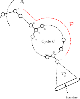
Figure 3: “Unicyclic Block”.

J.2.1 Proof of Lemma 47

Using the same arguments as for (143) in the proof of Lemma 45 , we get that

$$Q_{z_{i}}(\mathbf{T}^{j}_{x}) \leq n^{2}\max_{\mathcal{P}^{\prime}=(u_{0}=z,u_{1},\dots,u_{\ell})}\sum_{j=0}^{\ell}p_{u_{j}}\cdot\mathrm{deg}_{out}(u_{j})\prod_{i=0}^{j-1}p_{u_{i}}\times\left[\mathrm{deg}(u_{i})-\mathrm{deg}_{out}(u_{i})\right]\qquad$$ (152)

$$\leq n^{2}\ \widehat{d}\ \max_{\mathcal{P}^{\prime}=(u_{0}=z,u_{1},\dots,u_{\ell})}\sum_{j=0}^{\ell}p_{u_{j}}\prod_{i=0}^{j-1}p_{u_{i}}\times\left[\mathrm{deg}(u_{i})\right],\qquad$$

where the last inequality follows from the fact that $0\leq\mathrm{deg}_{out}(u_{j})\leq\widehat{d}$, for any $u_{j}$.

Let ${\cal P}_{z}=\{w_{0}=z,\ldots,w_{\ell}\}$ be the path that maximizes the r.h.s. of (152). Also let

$$\textstyle\mathbold{R}(j)=p_{w_{j}}\prod_{i=0}^{j-1}p_{w_{i}}\times\left[\mathrm{deg}(w_{i})\right].$$

That is, $\mathbold{R}(j)$ is the $j$-th sumad in (152). Let $M$ be the set of high degree vertices in the subpath of ${\cal P}_{z}$, $w_{0},\ldots,w_{j}$. Also let $m=|M|$. It holds that

$$\mathbold{R}(j) \leq \textstyle\left(\frac{1}{1+\epsilon/5}\right)^{j-m}\prod_{w\in M}\mathrm{deg}(w).$$ (153)

So as to compute $\prod_{w\in M}\mathrm{deg}(w)$ we use Corollary 12 and get that

$$\textstyle\prod_{w\in M}\mathrm{deg}(w)\leq d^{-15m}\left(1+\epsilon/10\right)^{\ell+j-(h+m)}\left(\prod_{w\in H}d^{15}\ \mathrm{deg}(w)\right)^{-1}.$$

Plugging the above into (153) we get that

$$\mathbold{R}(j) \leq \textstyle\left(1-2\epsilon/3\right)^{j-m}d^{-15m}\left(1+\epsilon/10\right)^{\ell-h}\left(\prod_{w\in H}d^{15}\ \mathrm{deg}(w)\right)^{-1}$$

$$\leq \textstyle\left(1-2\epsilon/3\right)^{j}\left(1+\epsilon/10\right)^{\ell-h}\left(\prod_{w\in H}d^{15}\ \mathrm{deg}(w)\right)^{-1}.$$

In the above bound for $\mathbold{R}(j)$, the only quantity that depends on $j$ is $(1-2\epsilon/3)^{j}$. We have that

$$Q_{z_{i}}(\mathbf{T}^{j}_{x}) \leq n^{2}\textstyle\sum_{j\geq 0}\mathbold{R}(j)\ \leq\ \frac{3}{2\epsilon}\left(1+\epsilon/10\right)^{l-h}\left(\prod_{w\in H}d^{15}\ \mathrm{deg}(w)\right)^{-1}.$$

The lemma follows.

Appendix K Proof of Lemma 3

First we show that typical instances of $G(n,d/n)$ admit a block partition ${\cal B}(\epsilon,d,\Delta)$. Given $\epsilon>0$, consider the graph $G\sim G(n,d/n)$ for sufficiently large $d>0$. We use the weighting schema in (1) and (2) to specify the breakpoints. At this point we introduce the notion of “influence path”.

Definition 4.

The path $L$ is called “influence path” only if none of its vertices is a breakpoint.

If vertex $w_{1}$ is a breakpoint, we define that there is only one influence path that starts from $w_{1}$, this is the trivial path $L={w_{1}}$.

The following result which implies that typically $G(n,d/n)$ does not have long influence paths. We call elementary every path $L=w_{1},\ldots,w_{\ell}$ such that there is no other path $P$ of length less than $10\frac{\ln n}{d^{4/5}}$ which connects any two vertices in $L$.

Theorem 48 (Efthymiou [10]).

Let $\epsilon\in(0,3/2)$. For large $d$, consider $G\sim G(n,d/n)$. Let $\mathbf{U}$ be the set of the elementary paths in $G$ of length $\frac{\ln n}{(\ln d)^{5}}$ that do not have any $r$-breakpoint for $r=\log n/d^{4/5}$. It holds that $\Pr[\mathbf{U}\neq\emptyset]\leq 4n^{(-\frac{1}{2}\ln d+2)}.$

Furthermore, we use the following result from [10].

Lemma 49.

Let $\epsilon\in(0,3/2)$. For large $d$, consider $G\sim G(n,d/n)$. With probability at least $1-2n^{-\frac{d^{2/5}}{2}}$ over the graph instances the following is true: Every vertex $v$ which is $r$-breakpoint for $r=\log n/d^{4/5}$, it is, also, a $r^{\prime}$-breakpoint for $r^{\prime}=10\log n$.

The proof of Lemma 49 is the same as the proof of Lemma 3 in [10].

Let ${\cal C}$ be the set of all cycles of length at most $4\frac{\ln n}{(\ln d)^{5}}$ in $G$. We need to argue that any two cycles in ${\cal C}$ are far apart from each other. In particular, we have the following result:

Lemma 50.

With probability at least $1-10n^{-3/4}$ over the instances of $G(n,d/n)$, any two cycles in ${\cal C}$ are at distance greater than $10\frac{\log n}{(\log d)^{5}}$.

Proof.

If there is a pair of cycles in ${\cal C}$ at distance less than $10\frac{\ln n}{(\ln d)^{5}}$, then the following should hold: There is a set of vertices $S$ of cardinality less than $2\frac{\ln n}{(\ln d)^{2}}$ such that the number of edges between the vertices in $S$ is at least $|S|+1$. We show that such a set does not exist in $G(n,d/n)$ with probability at least $1-n^{-3/4}$.

Let $D$ be the event that such a set exists. It holds that

$$\Pr[D] \leq \sum_{r=1}^{2\frac{\ln n}{(\ln d)^{2}}}{n\choose r}{{r\choose 2}\choose r+1}\left(\frac{d}{n}\right)^{r+1}\leq\sum_{r=1}^{2\frac{\ln n}{(\ln d)^{2}}}\left(\frac{ne}{r}\right)^{r}\left(\frac{r^{2}e}{2(r+1)}\right)^{r+1}\left(\frac{d}{n}\right)^{r+1}\hskip 21.33955pt\textstyle\left[\textrm{as }{n\choose r}\leq\left(\frac{ne}{r}\right)^{r}\right]$$

$$\leq \frac{1}{n}\sum_{r=1}^{2\frac{\ln n}{(\ln d)^{2}}}\left(\frac{erd}{2}\right)\left(\frac{e^{2}d}{2}\right)^{r}\leq\frac{ed}{(\ln d)^{2}}\ \frac{\ln n}{n}\sum_{r=1}^{2\frac{\ln n}{(\ln d)^{2}}}\left(\frac{e^{2}d}{2}\right)^{r}\hskip 89.626pt\mbox{[as $r\leq 2\ln n/(\ln d)^{2}$]}$$

$$\leq n^{-9/10}\left({e^{2}d}/{2}\right)^{2\frac{\ln n}{(\ln d)^{2}}}\leq n^{-3/4}.$$

The lemma follows ∎

Finally we use the following standard result, for a proof see e.g. in [14], in Section 3.

Lemma 51.

Let $\Delta$ be the maximum degree in $G(n,d/n)$. It holds that

$$\Pr[\Delta\geq(3/2)\log n/\log\log n]\leq n^{-1/4}.$$

We are going to show that $G$ admits the partition ${\cal B}={\cal B}(\epsilon,d,\Delta)$ if (a) the maximum degree $\Delta$ is less than $(3/2)\log n/\log\log n$, (b) the distance between any two cycles in ${\cal C}$ is at least $10\log n/(\log d)^{5}$, (c) there are no elementary paths of length $\log n/(\log d)^{5}$ which do not contain a $r$ breakpoint for $r=\log n/d^{4/5}$ and (d) every $r$ breakpoint in $G$ is also an $r^{\prime}$ breakpoint for $r=10\log n$. From Lemmas 49, 50, 51 and Theorem 48, $G$ satisfies these properties with probability $1-o(1)$.

Let ${\cal H}$ be the set of breakpoints in $G$. Given the sets ${\cal H}$ and ${\cal C}$ we specify the set of block ${\cal B}$ as follows: For the cycle $C\in{\cal C}$ we create the block $B_{C}$. Let $\partial^{r}C$ contain all the vertices which are at distance $r=\textstyle\max\left\{2\log(|C|\ \Delta),\ \frac{\log\log d}{\log d}\left({|C|+\log\Delta}\right)\right\}$. Note that we always have $r\leq 5\frac{\log\log d}{(\log d)^{6}}\log n$. The block $B_{C}$ contains all the vertices in the cycle $C$ and $\partial^{r}C$. Additionally the block $B_{C}$ contains every vertex $w$ for which there is an influence path from $w$ to $\partial^{r}C$. We repeat the above process for every cycle in ${\cal C}$. Note that our assumptions about $G$ imply that the blocks created for each cycle are vertex disjoint.

Having specified the blocks which correspond to the cycles in ${\cal C}$, there are vertices whose block has not been specified yet. For each such vertex $w$ we specify its block $B_{w}$ by working as follows: The block $B_{w}$ contains $w$ and every $u$ which is reachable from $w$ through an influence path. The block construction ends once we have specified the block for all vertices in $G$. Note that if $w$ is a breakpoint then $B_{w}$ is a single vertex block. This follows from the definition of influence path.

In the following result we show that the blocks in ${\cal B}$ have the structured we promised.

Lemma 52.

For $\epsilon,d$ as specified in the statement of Lemma 3, consider the graph $G$ which admits the block partition as we described above. Additionally, assume that $G$ is such that

1. the distance between any two cycles in ${\cal C}$ is at least $10\log n/(\log d)^{5}$

2. there are no elementary paths of length $\log n/(\log d)^{5}$ which do not contain a breakpoint.

Then, the set of blocks ${\cal B}$ contains only blocks which are trees with one extra edge.

Proof.

Let ${\cal B}_{1}$ be the set of blocks created from the cycles in ${\cal C}$ and let ${\cal B}_{2}={\cal B}\backslash{\cal B}_{1}$. It suffices to show that ${\cal B}_{1}$ contains only unicyclic blocks and ${\cal B}_{2}$ contains only trees.

First we focus on ${\cal B}_{1}$. The assumption that there are no elementary paths of length $\log n/(\log d)^{5}$ which do not contain a breakpoint implies the following: There is no vertex $w$ at distance more than $(3/2)\log n/(\log d)^{5}$ from a cycle $C\in{\cal C}$ such that both $w$ and $C$ belong to the same block. Then, the assumption that for any two cycles in ${\cal C}$ their distance is at least $10\log n/(\log d)^{5}$ implies that for any two cycles $C_{1},C_{2}\in{\cal C}$ the corresponding blocks do not intersect.

So as to show that ${\cal B}_{2}$ consists of tree-like blocks we work as follows: Let some $B\in{\cal B}_{2}$ and let $w$ be the vertex we used to created it. It is direct that every path that connects $w$ to some vertex in any of the blocks in ${\cal B}_{1}$ should contain at least one breakpoint (otherwise $w$ should belong to a block in ${\cal B}_{1}$). That is, if $B$ contains a cycle $C$, then $C\notin{\cal C}$. This implies that $|C|>4\frac{\ln n}{(\ln d)^{5}}$. It suffices to show that every $B\in{\cal B}_{2}$ cannot contain a cycle of length $\ell\geq 3\frac{\ln n}{(\ln d)^{5}}$. But the second assumption about $G$ implies that the maximum cycle in $B$ is $2\log n/(\log d)^{5}$. This implies that $B$ cannot contain any cycle. We conclude that ${\cal B}_{2}$ contains only blocks which are trees.

The lemma follows. ∎

So as to show that $G$ admits the block partition ${\cal B}(\epsilon,d,\Delta)$, it suffices to show that the graph $G$ (and the set of blocks ${\cal B}$) has the following properties:

1. for each multi-vertex block $B\in{\cal B}$, each $u\in\partial_{\mathrm{out}}B$ is $r$-breakpoints for $r\geq{\max\{{\tt diam}(B),\log\log n\}}$

2. for each multi-vertex block $B$, each vertex in $\partial_{\mathrm{out}}B$ has exactly one neighbor inside $B$

3. if $B$ contains a cycle $C$, we have that ${\tt dist}(v,C)\geq\max\left\{2\log(|C|\ \Delta),\ \frac{\log\log d}{\log d}\left({|C|+\log\Delta}\right)\right\}$, for every $v\in\partial_{\mathrm{out}}B$

4. every $v\in{\partial{\cal B}}$ does not belong to any cycle of length less than $d^{2}$.

We start by arguing about (1). First, we show that $\partial_{\mathrm{out}}B$ consists of $r$-breakpoints for $r=10\log n$. Assume that some vertex $u\in\partial_{\mathrm{out}}B$ is not a $r$ breakpoint. W.l.o.g. assume that this block is a tree. Let $w$ be the vertex that is used to specify the block $B$. Since we assume that $B$ is multi-vertex $w$ is not a breakpoint. Furthermore, since $u\in\partial_{\mathrm{out}}B$ is not a breakpoint there should be an influence path from $w$ to $u$. In turn, this implies that $u$ should be included into $B$ during the construction of $B$. Clearly, this is a contradiction since $u$ was assumed to be in $\partial_{\mathrm{out}}B$. Then, (1) follows by noting that the diameter of $B$ is always less than $10\log n$.

For showing (2) we use proof by contradiction, as well. Assume that we have a multi-vertex block $B$ and there is $u\in\partial_{\mathrm{out}}B$ which has at least two neighbors inside $B$. Consider first the case where $B$ was created by a single vertex $w$. The block that is created by a single vertex cannot intersect with a cycle of length less than $4\log n/(\log d)^{5}$ However, if there exists such $u\in\partial_{\mathrm{out}}B$ then there should be a cycle of length less than $(5/2)\log n/(\log d)^{5}$ that intersects with the block $B$. Clearly this cannot be the case since we assumed that the block is created by a single vertex and not a short cycle. If on the other hand the block $B$ started from a cycle $C\in{\cal C}$, then the fact that there exists $u\in\partial_{\mathrm{out}}B$ implies that there two cycles of length less than $4\log n/(\log d)^{5}$ whose distance is much less than $(3/2)\log n/(\log d)^{5}$. This is a contradiction, since we assumed that any two cycles in ${\cal C}$ are at greater distance.

As far as (3) is concerned, consider the block construction for a block which includes a cycle $C\in{\cal C}$. In such a block we always add the vertex sets $\partial^{r}C$ in the block. The assumption that $\Delta=(3/2)\log n/\log\log n$ and the fact that the length of the cycle $C$ is at most $\log n/(\log d)^{5}$ imply that the addition of the set of vertices $\partial^{r}C$ into the block guarantees that (3) is satisfied.

Finally, for (4) we only need to observe that every $v$ in the outer boundary of a block cannot belong to a cycle in ${\cal C}$.

We, also, need to show for $k\geq\alpha d$, with high probability over the instances of $G(n,d/n)$, the graph can be colored using at least $k\geq\alpha d$ colors and the state space is connected. As far as the $k$-colorability of $G(n,d/n)$, for $k\geq\alpha d$, is regarded we use the result from [2, 6], i.e., with probability $1-o(1)$ the chromatic number of $G(n,d/n)$ is $d/(2\ln d)$.

From [7] we have that the Glauber dynamics (and hence the block dynamics) is ergodic with probability $1-o(1)$ over the instances $G(n,d/n)$ when $k\geq d+2$. For the sake of completeness let us sketch the proof for ergodicity in [7]. It is shown that if a graph $G$ has no $t$-core, then for all $k\geq t+2$ the Glauber dynamics for $k$-coloring yields an ergodic Markov chain (Lemma 2 in [7]). Then the authors use the result in [31], which states that w.h.p. $G(n,d/n)$ has no $t$-core for $t\geq d$.

We consider the claim about the size of the blocks. The fact that the vertices in $\partial_{\mathrm{in}}B$, for every $B\in{\cal B}$, are next to a break-point and Lemma 11 imply the following: for each $w\in\partial_{\mathrm{in}}B$ the number of vertices that are at distance $\ell$ from $w$ is less than $[(1+\epsilon)d]^{\ell}$. Then, the result follows easily one we note that the diameter of each block in ${\cal B}$, given that $\Delta=\Theta(\log n/(\log\log n))$, is less than $10\log n/\log^{4}d$.

Appendix L Hard-Core Model - Analysis for Rapid Mixing

In this section we show the following result:

Theorem 53.

For all $\epsilon>0$, there exists $d_{0}>1$, for all $d>d_{0}$, for $\lambda\leq(1-\epsilon)/d$, there exists $C=C(d)>0$ such that with probability $1-o(1)$ over the choice of $G\sim G(n,d/n)$, the mixing time of the Glauber dynamics is $O(n^{C})$.

So as to get Theorem 53 first we prove the following result that concerns block dynamics.

Theorem 54.

For all $\epsilon,\Delta>0$, there exists $C,d_{0}>0$ such that for all $d\geq d_{0}$, and any graph $G$ which admits block partition ${\cal B}={\cal B}(\epsilon,d)$ the following is true: For $\lambda\leq(1-\epsilon)/d$, the block dynamics with set of block ${\cal B}$ has mixing time

$$T_{\mathrm{mix}}\leq Cn\log n.$$

Additionally to Theorem 54 we have the following result.

Lemma 55.

For all $\epsilon>0$ and $\Delta=(3/2)\left(\log n/\log\log n\right)$, there exists $d_{0}>0$ such that for all $d\geq d_{0}$ $G(n,d/n)$ admits the block partition ${\cal B}={\cal B}(\epsilon,d,\Delta)$.

The proof of Lemma 55 is almost identical to that of Lemma 3. For this reason we omit it.

In light of Theorem 54 and Lemma 55, Theorem 53 follows by utilizing a standard comparison argument, see Section M.

We proceed with the proof of Theorem 54. First we note that for any $\lambda>0$ the dynamics is trivially ergodic for any $G$ which admits a block partition ${\cal B}(\epsilon,d,\Delta)$. This follows from the observation that from every independent set of $G$ there is a sequence of transitions to the empty independent set, each with positive probability, and the other way around.

For showing the rapid mixing result for the hard-core model it suffices to show that in the block dynamics the blocks are always in a convergent configuration. Then rapid mixing follows by using Theorem 13 and standard arguments, almost identical to those we use for Theorem 4.

Corollary 56.

For all $\epsilon>0$, $\Delta>0$, there exists $d_{0}>0$ such that for any $d\geq d_{0}$, for every graph $G$ which admits block partition ${\cal B}(\epsilon,d,\Delta)$, and any $v\in{\partial{\cal B}}$ the following is true:

Let $(X_{t})_{t\geq 0},(Y_{t})_{t\geq 0}$ be two copies of the block dynamics on the hard-core model on $G$ such that for some $t\geq 0$ we have $X_{t}\oplus Y_{t}=\{u^{*}\}$. For any $B$ such that $u^{*}\in\partial_{\mathrm{out}}B$ and any vertex $w\in B$ we have that the probability of propagation $p_{w}<(1-\epsilon)/d$.

Proof.

Let $(X_{t})_{t\geq 0},(Y_{t})_{t\geq 0}$ be two copies of the block dynamics on the hard-core model on $G$ such that for some $t\geq 0$ we have $X_{t}\oplus Y_{t}=\{u^{*}\}$. Consider some block $B$ such that $v\in\partial_{\mathrm{out}}B$. Then, so as to bound the probability of propagation for each vertex $u$ note the following: Assume that the vertex $w$ is disagreeing, w.l.o.g. assume that $X_{t+1}(w)$ is occupied, i.e., $w$ belongs to the independent set, and $Y_{t+1}(w)$ is unoccupied. Clearly $X_{t+1}(u)$ cannot become occupied. The only way we can have disagreement at $u$, is when all the neighbours of $u$, apart from $w$, in both configurations are unoccupied. Then, $Y_{t+1}(u)$ becomes occupied (disagreeing) with probability $\frac{\lambda}{1+\lambda}$.

Choosing $\lambda\leq(1-\epsilon)/d$, the above remarks implies that the probability of propagation is less than $(1-\epsilon)/d$, always. ∎

In light of Corollary 56, Theorem 54 follows.

Appendix M Rapid Mixing for Single Site Dynamics - The Comparison

In this section we show that the rapid mixing result we get for the block dynamics for coloring imply Theorem 1. Similarly, for the hard-core model, i.e., Theorem 53. In a lot of our results in this section we need to use continuous time Markov chains, rather than discrete time. In the continuous time block dynamics each block is updated according to an independent Poisson clock with rate 1.

We use the following comparison result from [27], which in our context writes as follows:

Proposition 57.

Consider some graph $G$. Let $(X_{t})_{t\geq 0}$ be the continuous time block dynamics, with set of blocks ${\cal B}$, where each vertex $v$ belongs to $Q_{v}$ different blocks. Also, let $(Y_{t})_{t\geq 0}$ be the continuous time single site dynamics on $G$. Let $\tau_{block},\tau$ be the relaxation times of $(X_{t})$ and $(Y_{t})$, respectively. Furthermore, for each block $B\in{\cal B}$ let $\tau_{B}$ be the relaxation time of the continuous time single site dynamics on $B$, given any arbitrary condition at $\partial_{\mathrm{out}}B$. Then we have that

$$\tau\leq\tau_{block}(\max_{B\in{\cal B}}\tau_{B})(\max_{v}Q_{v}).$$

For some $G\in{\cal F}(\epsilon,d,\Delta)$, with block partition ${\cal B}$, let ${\cal P}$ be the set of paths which connect either a high degree vertex or the cycles in the block $B$ (if any) to $\partial_{\mathrm{in}}B$.

We show rapid mixing for the single site Glauber dynamics of $G(n,d/n)$ if, additionally to the condition $G(n,d/n)\in{\cal F}(\epsilon,d,\Delta)$, for $\Delta=(3/2)\log n/(\log\log n)$, the graph, also, satisfies the following one: For each path $P\in{\cal P}$ let

$${\cal J}(P)=450\sum_{u\in P}\left(\log(\mathrm{deg}(u))+{\mathrm{deg}(u)}/{k}\right).$$

The additional property is that every path $P\in{\cal P}$ is such that

$${\cal J}(P)\leq 10^{4}\log n/(\log d)^{2}.$$ (154)

where $|P|$ is the number of vertices in $P$.

For some $\epsilon,d,\Delta>0$, let ${\cal L}(\epsilon,d,\Delta)$ be the family of graphs $G$ such that $G\in{\cal F}(\epsilon,d,\Delta)$ and every $P\in{\cal P}$ satisfies (154).

Lemma 58.

For $\epsilon,d$ and $\Delta$ as in Lemma 3, with probability $1-o(1)$ over the graph instances we have that $G(n,d/n)\in{\cal L}(\epsilon,d,\Delta)$.

The proof of Lemma 58 appears in Section O.

For $\epsilon,d$ and $\Delta$ as in Lemma 3, consider some graph $G\sim G(n,d/n)$ such that $G\in{\cal L}(\epsilon,d,\Delta)$. Let $(X_{t})_{t\geq 0}$ be the continuous time, block dynamics, with set of blocks ${\cal B}$. Also, let $(Y_{t})_{t\geq 0}$ be the continuous time single site dynamics on $G$. Theorem 2 and Lemma 3 imply that choosing $k\geq(\alpha+\epsilon)d$, for $\tau_{block}$, the relaxation time of $(X_{t})_{t\geq 0}$, we have that

$$\tau_{block}=O\left(\log n\right).$$ (155)

Lemma 59.

For every $B\in{\cal B}$ consider the continuous time, single site dynamics $(X^{B}_{t})_{t\geq 0}$ over the $k$-colorings of $B$ with arbitrary boundary condition at $\partial_{\mathrm{out}}B$. Let $\tau_{B}$ be the relaxation time of $(X^{B}_{t})_{t\geq 0}$. For any $k\geq(\alpha+\epsilon)d$ it holds that

$$\tau_{B}\leq n^{2/(\log d)^{2}}.$$

The proof of Lemma 59 appears in Section M.1.

Combining (155) with Lemma 59 and Proposition 57 we get the following: letting $\tau_{cont}$ be the relaxation time $(Y_{t})_{t\geq 0}$ for $k\geq(\alpha+\epsilon)d$, we have that

$$\textstyle\tau_{\rm cont}=O\left(n^{2/(\log d)^{2}}\log n\right)=O\left(n^{3/(\log d)^{2}}\right).$$

Now, let $(Z_{t})_{t\geq 0}$ be the discrete time, single site Glauber dynamics on the $k$-colorings of $G$ with $k\geq(\alpha+\epsilon)d$. Let $\tau_{\rm disc}$ and $T_{\rm mix}$ be the relaxation time and the mixing time of $(Z_{t})_{t\geq 0}$, respectively. The above bound for $\tau_{cont}$ implies that $\tau_{disc}\leq n^{1+3/(\log d)^{2}}.$ Then, it is standard that $\textstyle T_{mix}=O\left(n^{2+3/(\log d)^{2}}\right).$ Theorem 1 follows.

As far as the hard-core model is regarded, we show the following result.

Lemma 60.

For every $B\in{\cal B}$ consider the continuous time, single site dynamics $(X^{B}_{t})_{t\geq 0}$ for the hard-core model of $B$ with arbitrary boundary condition at $\partial_{\mathrm{out}}B$. Let $\tau_{B}$ be the relaxation time of $(X^{B}_{t})_{t\geq 0}$. For any $\lambda\leq(1-\epsilon)/d$ there exists $C_{1}>0$ which depends on $\epsilon,d$, such that $\tau_{B}\leq n^{C_{1}}.$

In light of Claim 68, Lemma 60 follows directly from Theorem 4.2 and Lemma 4.1 and 4.4 in [30].

Theorem 54 follows by combining Lemma 60 with arguments which are very similar to those we used for the coloring model.

M.1 The relaxation time for the blocks - Proof of Lemma 59

We proceed by bounding appropriately the quantities $\tau_{B}$ for every $B\in{\cal B}$. As discussed earlier, the blocks of $G$ are trees with at most one extra edge.

Definition 5.

For a tree $T$ rooted at $v$, let the maximal path density be defined as $m(T,v)=\max_{P}{\cal J}(P)$, where the maximum is over all the paths $P$ in $T$ which start from $v$.

For a graph $G\in{\cal L}(\epsilon,d,\Delta)$, with block partition ${\cal B}$, let ${\cal T}={\cal T}(G,{\cal B})$ be the family which contains the following rooted trees, subgraphs of $G$: ${\cal T}$ includes all the tree-like, multi-vertex blocks in ${\cal B}$. The root of each tree is a high degree vertex (any) inside the block. Also, for each $B\in{\cal B}$ that is unicyclic with cycle $C=w_{1},\ldots,w_{\ell}$ , the set ${\cal T}$ contains every subtree $T_{i}$ that hang from the cycle. That is, for $i=1,\ldots,\ell$, $T_{i}$ is the induced subgraph of $B$ that corresponds to the set of vertices in the connected component of $B$ that contains vertex $w_{i}$ once we delete all the edges of $C$. The root for $T_{i}$ is the vertex $w_{i}$. For each $T\in{\cal T}$which belongs to the block $B$, we let $\partial_{\mathrm{out}}T$ be the set of vertices in $\partial_{\mathrm{out}}B$ which are incident to $T$.

The following result relates the relaxation times of the trees in ${\cal T}$ and their, corresponding, maximal path density.

Theorem 61.

For any $\epsilon,\Delta>0$ and sufficiently large $d>0$ let $k\geq(\alpha+\epsilon)d$. Consider $G\in{\cal F}(\epsilon,d,\Delta)$ and block partition ${\cal B}$. For any $T\in{\cal T}$, with root $v$, and boundary condition $\sigma(\partial_{\mathrm{out}}T)$, the relaxation time $\tau_{\rm rel}$ of the Glauber dynamics, we have $\tau_{\rm rel}(T)\leq\exp\left(m(T,v))\right).$

The proof of Theorem 61 appears in Section N.

From Lemma 58 and Theorem 61 we get that if $G(n,d/n)\in{\cal L}(\epsilon,d,\Delta)$, where $\epsilon$, $d$ and $\Delta$ are as in Lemma 3, then the continuous time Glauber dynamics on $T\in{\cal T}(G(n,d/n),{\cal B})$ exhibits relaxation time

$$\tau_{\rm rel}(T)\leq n^{1/(\log d)^{2}}.$$ (156)

The above implies that for a tree-like block $B\in{\cal B}$ the lemma is true.

Consider the unicyclic block $B$ with arbitrary boundary condition at $\partial_{\mathrm{out}}B$. Let $C=w_{1},\ldots,w_{\ell}$ be the cycle inside $B$, for some $\ell\leq\log n/(\log d)^{5}$. Consider $(Z^{B}_{t})_{t\geq 0}$ the continuous time, block dynamics, on $B$ with arbitrary boundary condition at $\partial_{\mathrm{out}}B$. The set of blocks is the subtrees $T\in{\cal T}$ which intersect with the cycle $C$. Using path coupling and Proposition 19 it is elementary to show that the relaxation time of the block dynamics $\tau_{B}\leq 10\log|C|=O(\log\log n)$.

Let $(X_{t})_{t\geq 0}$ be the Glauber dynamics on $B$ with arbitrary boundary at $\partial_{\mathrm{out}}B$. The bound on relaxation time for $(Z^{B}_{t})_{t\geq 0}$, combined with (156) and Proposition 57, imply that the relaxation time for $(X_{t})$ is such that $\tau_{B}=O\left(n^{1/(\log d)^{2}}\log\log n\right)\leq O\left(n^{2/(\log d)^{2}}\right)$. The lemma follows

Appendix N Proof of Theorem 61

For the tree $T$ and some vertex $u\in T_{u}$, let $T_{u}$ denote the subtree of $T$ which contains $u$ and all its descendants. Unless otherwise specified, we assume that the root of $T_{u}$ is $u$. Also, for a boundary set $\partial_{\mathrm{out}}T$ of $T$, we let $\partial_{\mathrm{out}}T_{u}$ contain every $w\in\partial_{\mathrm{out}}T$ which is a boundary at $T_{u}$, as well.

We also have the following result whose proof appears in Section N.1.

Proposition 62.

For $\epsilon,d,\Delta,k$ as in Theorem 61 the following is true:

Let $T\in{\cal T}$ and let $v\in T$. Consider $T_{u}$ and let $w_{1},\ldots,w_{R}$ be the children of the root, where $R=\mathrm{deg}(v)$. Consider the block dynamics with set of blocks ${\cal M}=\{\{v\},T_{w_{1}},\ldots,T_{w_{R}}\}$. Assume that for any $\sigma(\partial_{\mathrm{out}}T)$, any $v\in\{u,w_{1},\ldots,w_{\ell}\}$ for the random coloring $Z$ we have

$$\left|\Pr[Z(v)\ |\ Z(\partial_{\mathrm{out}}T)=\sigma(\partial_{\mathrm{out}}T)]-1/k\right|\leq 100/k^{2}.$$ (157)

Then, under any boundary condition at $\partial_{\mathrm{out}}T$, the block dynamics $(X_{t})_{t\geq 0}$ exhibits

$$\tau_{\rm rel}(T_{u})\leq(10R^{2}\log R)^{15}\exp\left(450R/k\right).$$

For any $T\in{\cal T}$ and any $u\in T$, Proposition 21 implies that if $u$ is a high-degree vertex or it is a low-degree vertex which is adjacent to high degree vertices then the spatial mixing assumption (157) is true. We also have the following result whose proof appears in Section .N.2.

Lemma 63.

For $\epsilon,d,\Delta,k$ as in Theorem 61 the following is true:

Let $T\in{\cal T}$ and let $v\in T$. Consider $T_{u}$ and let $w_{1},\ldots,w_{R}$ be the children of the root, where $R=\mathrm{deg}_{in}(v)$. Let $(X_{t})_{t\geq 0}$ be the block dynamics with set of blocks ${\cal M}=\{\{v\},T_{w_{1}},\ldots,T_{w_{R}}\}$. Assume that the degrees of $v,w_{1},\ldots,w_{R}$ are at most $\widehat{d}$.

Under any boundary condition at $\partial_{\mathrm{out}}T_{u}$, $(X_{t})_{t\geq 0}$ exhibits

$$\tau_{\rm rel}(T_{u})\leq 10^{4}\exp\left(5\max\{\log(R/(k-\widehat{d})),5\}\right)\log R$$

Note that Lemma 63 includes the case where $u$ is such that $\mathrm{deg}_{out}(u)>0$, i.e., some of the neighbors of $u$ belong to $\partial_{\mathrm{out}}T_{u}$ and have frozen color assignment. Unifying Lemma 63 and Proposition 62, we get the following: for any $T\in{\cal T}$ and any $u\in T$ we have that

$$\tau_{\rm rel}(T_{u})\leq\exp\left(450\left(\log(\mathrm{deg}(v))+{\mathrm{deg}(u)}/{k}\right)\right).$$ (158)

In light of (158), Theorem 61 follows by combining a simple induction and Proposition 57. Consider $T\in{\cal T}$. If $T$ is a single vertex, then $\tau_{\rm rel}(T)=1$. Assume, now, that the root $v$ of $T$ has children $w_{1},\ldots,w_{\ell}$, for some $\ell>0$. Then by the induction hypothesis we have that

$$\tau_{\rm rel}(T_{w_{i}})\leq\exp\left(m(T_{w_{i}},w_{i})\right)\qquad\textrm{ for $i=1,\ldots,\ell$}.$$ (159)

Consider the block dynamics on $T$ where the blocks are, the root $v$ and the subtrees $T_{w_{i}}$. The relaxation time for this process is given by (158). The theorem follows from (158), (159) and Proposition 57.

N.1 Proof of Proposition 62

Let $(X_{t}),(Y_{t})$ be two copies of the discrete time block dynamics such that $X_{0},Y_{0}$ are arbitrary $k$-colorings of $T$. We present a coupling such that after $R^{5}\exp\left(100R/k\right)$ steps the probability of the event $X_{t}\neq Y_{t}$ is less than $e^{-1}$.

The coupling is such that we update the same block at each copy of the dynamics. When we update a block are couple the configurations maximally, i.e., when we update block $B$ at time $t$, we minimize the probability of the event $X_{t}(B)\neq Y_{t}(B)$.

Let $t_{1},t_{2},\ldots$ be the random times at which $u$ is updated in the coupling. For $i\geq 1$, we say that $t_{i}$ is a “success” if the following hold:

1. $|t_{i+1}-t_{i}|\geq 3R\max\{\log(R/k),5\}$

2. we have that

   • $|A_{X_{t_{i}}}(u)\oplus A_{Y_{t_{i}}}(u)|\leq 10$

   • $\min\{|A_{X_{t_{i}}}(u),A_{Y_{t_{i}}}(u)\}\geq 100$

3. the number of vertices $w_{j}$ such that $X_{t_{i}}(w_{j})\neq Y_{t_{i}}(w_{j})$ is less than $100R/k$.

Claim 64.

If $t_{i}$ is a success, for $i\geq 1$, then there is a coupling such that $\Pr\left[X_{t_{i+1}}\neq Y_{t_{i+1}}\right]\leq e^{-2}.$

Proof.

Consider the time interval ${\cal I}(t_{i},t_{i+1})$. Note that if $X_{t_{i}}(v)=Y_{t_{i}}(v)$, then in the time interval ${\cal I}$ at every update of the block $T_{w_{j}}$ can be done by using identical coupling. This means that for every $w_{j}$ whose block is updated at least once during ${\cal I}$ we have $X_{t_{i+1}}(w_{j})=Y_{t_{i+1}}(w_{j})$. Thus, if there exists $w_{j}$ such that $X_{t_{i+1}}(w_{j})\neq Y_{t_{i+1}}(w_{j})$, then this must have been a disagreement created at some $t<t_{i}$ and survived during the time interval ${\cal I}$.

Let $W$ be the number of children $w_{i}$ which disagree at time $t_{i}$ and they are not updated during the interval ${\cal I}$. If there are no such disagreements we set $W=0$. Clearly it holds that

$$\Pr[X_{t_{i+1}}=Y_{t_{i+1}}]\leq\Pr[X_{t_{i}}(u)=Y_{t_{i}}(u),W=0]=\Pr[W=0\ |\ X_{t_{i}}(u)=Y_{t_{i}}(u)]\Pr[X_{t_{i}}(u)=Y_{t_{i}}(u)].$$ (160)

Our assumption that $t_{i}$ is success implies that

$$\Pr[X_{t_{i}}(u)\neq Y_{t_{i}}(u)]\leq 1/10.$$ (161)

Note that each block $T_{w_{j}}$ such that $X_{t_{i}}(w_{j})\neq X_{t_{i}}(w_{j})$ is update during the time interval ${\cal I}$ with probability at least $1-\min\{(R/k)^{-2},e^{-15}\}$. Markov’s inequality imply that

$$\Pr[W>0\ |\ X_{t_{i}}(u)=Y_{t_{i}}(u)]\leq\min\{(R/k)^{-1},e^{-12}\}.$$ (162)

The result follows by plugging (161) and (162) into (160). ∎

We also have the following result whose proof appears in Section N.1.1.

Lemma 65.

For any $t_{i}\geq 3R\log R$ we have that $\Pr[\textrm{$t_{i}$ is success}]\geq\rho$, where

$$\rho\geq\exp\left(-15\max\{\log(R/k),5\}-450R/k\right).$$

Let $T=10^{4}\left\lceil\rho^{-1}R\log R\right\rceil$, where $\rho$ is defined in Lemma 65. We consider the time interval ${\cal I}=[0,T]$. We partition ${\cal I}$ into subintervals ${\cal I}_{0},{\cal I}_{1},\ldots$ each of length $4R\log R$. Lemma 65 implies that that the probability of having a success at ${\cal I}_{j+2}$ is at least $\rho$, regardless of what happens in ${\cal I}_{j}$.

Noting that the probability that $v$ is updated during ${\cal I}_{2j}$ is greater than $1/2$, the probability of having $t_{i}\in{\cal I}_{j}$ which is success is at least $\rho/2$.

Let ${\cal E}$ be the event that there exists $j\geq 1$ such that ${\cal I}_{2j}$ there exists $t_{i}$ which is success. Since there are at least $100/\rho$ subintervals to check, it is elementary to verify that

$$\Pr[{\cal E}]\geq 1-e^{-5}.$$ (163)

Let ${\cal C}$ be the event that in the coupling of $(X_{t})$ and $(Y_{t})$ there exists $t\in{\cal I}$ such that $X_{t}=Y_{t}$. Then, we have that

$$\Pr[{\cal C}]\geq\Pr[{\cal C}\ |\ {\cal E}]\Pr[{\cal E}]\geq(1-e^{-2})(1-e^{-5})\geq 1-e^{-1}.$$ (164)

In the above inequalities we substituted $\Pr[{\cal C}\ |\ {\cal E}]$ by using Claim 64 and $\Pr[{\cal E}]$ by using (163).

N.1.1 Proof of Lemma 65

Let ${\cal C}$ be the event that $|t_{i+1}-t_{i}|\geq 3R\max\{\log(R/k),5\}$. Also, let ${\cal D}$ be the event that $t_{i}$ satisfies the requirements 2 and 3 to be “success”. The lemma follows by noting that

$$\rho\geq\Pr[{\cal C}]\Pr[{\cal D}].$$ (165)

At each step the vertex $u$ is updated with probability $\frac{1}{R+1}$. Then we have

$$\Pr[{\cal C}]=\left(1-{1}/({R+1})\right)^{3R\max\{\log(R/k),5\}}\geq\exp\left(-4\max\{\log(R/k),5\}\right).$$ (166)

For computing $\Pr[{\cal D}]$ we consider cases regarding $R/k^{2}$ being larger or at most $10^{-4}$.

Claim 66.

For $R/k^{2}>10^{-4}$ we have that $\Pr[{\cal D}]\geq\exp\left(-450R/k\right)$.

Claim 67.

For $R/k^{2}\leq 10^{-4}$, we have that $\Pr[{\cal D}]\geq\exp\left(-10\max\{\log(R/k),5\}-400R/k\right)$

The lemma follows by plugging the bounds from (166) and Claims 66, 67 into (179).

It remains to show that Claims 66, 67 are indeed true.

Proof of Claim 66.

Let the interval ${\cal I}=[t_{i}-R,t_{i})$ and let the set $W=\{1,2,\ldots,100\}$. Consider the following events: let $\cal G$ be the event that for every $t\in{\cal I}$ we have $W\subseteq A_{X_{t}}(u),A_{Y_{t}}(u)$. That is, the first 100 colors are available for the root during the whole interval ${\cal I}$. Let ${\cal S}$ be the event that at time $t_{i}$ there are $q_{1},q_{2}\in[k]$ such that $A_{X_{t_{i}}}(u)=W\cup\{q_{1}\}$ and $A_{Y_{t_{i}}}(u)=W\cup\{q_{2}\}$. That is, the two sets differ only on at most two colors. Let ${\cal N}$ be the event that $u$ is not updated during interval ${\cal I}$. Finally let ${\cal Z}$ be the event that the number of disagreeing children of $u$ is at most $100R/k$.

It is direct that if the events ${\cal G}$, ${\cal N}$, ${\cal S}$ and ${\cal Z}$ hold then the event ${\cal D}$ holds. That is, $\Pr[{\cal D}]\geq\Pr[{\cal G},{\cal S},{\cal N},{\cal Z}]$. More specifically, we have

$$\Pr[{\cal D}]\geq\Pr[{\cal N}]\Pr[{\cal G}\ |\ {\cal N}]\Pr[{\cal S}\ |\ {\cal G},{\cal N}]\Pr[{\cal Z}\ |\ {\cal G},{\cal N},{\cal S}].$$ (167)

The claim follows by bounding appropriately the probability terms on the r.h.s. of (167).

We start with $\Pr[{\cal N}]$. Using standard coupon collector argument it is elementary to verify that

$$\Pr[{\cal N}]\geq e^{-2}.$$ (168)

We proceed by considering $\Pr[{\cal G}\ |\ {\cal N}]$. Conditional on ${\cal N}$, in the coupling of $(X_{t})$ and $(Y_{t})$ we have that updating block $T_{w_{j}}$, each color in $W$ is not used for both $X_{t}(w_{j})$ and $Y_{t}(w_{j})$ with probability at least $1-{2}/{k}$. Conditioning that all the blocks $T_{w_{j}}$s are updated prior to time $t_{i}-R$, consider the last time that each $T_{w_{j}}$ is updated prior to $t_{i}-R$. The probability that non of the colors in $W$ is used for the children $w_{1},\ldots,w_{R}$ at time $t_{i}-R$, is at least $\left(1-{200}/{k}\right)^{R}\geq\exp\left(-200R/k\right).$ The probability that non of the following $R$ updates uses any color from $W$ for $w_{1},\ldots,w_{R}$ is at least $\left(1-{200}/{k}\right)^{R}\geq\exp\left(-200R/k\right).$ From the above we conclude that

$$\Pr[{\cal G}\ |\ {\cal N},{\cal Q}]\geq\exp\left(-400R/k\right),$$

where ${\cal Q}$ is the event that there is no block $T_{w_{j}}$ which is not updated at least once prior to time $t_{i}-R$. Furthermore, we get that

$$\Pr[\bar{\cal Q}\ |\ {\cal N}]\leq\Delta\ \Pr[{T}_{w_{1}}\textrm{ is not updated by time }t_{i}-R\ |\ {\cal N}]\leq 2R^{-1},$$

since $t_{i}-R>2R\log R$. Or, $\Pr[{\cal Q}\ |\ {\cal N}]\geq 1/2$. We have that

$$\Pr[{\cal G}\ |\ {\cal N}]\ \geq\ \Pr[{\cal G}\ |\ {\cal N},{\cal Q}]\Pr[{\cal Q}\ |\ {\cal N}]\ \geq\ 2^{-1}\exp\left(-400R/k\right).$$ (169)

We proceed by considering $\Pr[{\cal S}\ |\ {\cal G},{\cal N}]$. Conditional on ${\cal N}$ and ${\cal G}$, at each block update $T_{w_{j}}$ some color $q$ is assigned to vertex $w_{j}$ with probability at most $2/k$. Assume that at time $t=t_{i}-\Delta$ we have $X_{t}(v)=q_{1}$ and $Y_{t}(v)=q_{2}$. For $(X_{t})$, we call available colors the set of colors $[k]\setminus(W\cup\{q_{1}\})$. Similarly, for $(Y_{t})$, we call available colors the set of colors $[k]\setminus(W\cup\{q_{2}\})$. Let $K$ be the number of colors which are available in some chain and they are not used from any of $w_{1},\ldots,w_{R}$ in the corresponding chain at time $t_{i}$.

Assume that at time $t\in{\cal I}$ we update block $T_{w_{j}}$. Recall that for any $t\in{\cal I}$ we have $X_{t}(v)=q_{1}$ and $Y_{t}(v)=q_{2}$. We couple $X_{t}(w_{j})$ and $Y_{t}(w_{j})$ such that for each $q\in[k]\setminus(W\cup\{q_{1},q_{2}\})$ we set $\Pr[X_{t}(w_{j})=Y_{t}(w_{j})=q]$ with probability $\min\{\Pr[X_{t}(w_{j})=q],\Pr[Y_{t}(w_{j})=q]\}$, while for the colors $q_{1},q_{2}$ we have $\Pr[X_{t}(w_{j})=q_{2},Y_{t}(w_{j})=q_{1}]$ with probability $\min\{\Pr[X_{t}(w_{j})=q_{2}],\Pr[Y_{t}(w_{j})=q_{1}]\}$. The aforementioned coupling is what we call, “maximal coupling”.

The above implies that if at time $t\in{\cal I}$ the coupling updates block $T_{w_{j}}$, each available color is used for $w_{j}$ with probability at most $2/k$. This implies that some available color is not used at all for coloring any of the vertices in $w_{1},\ldots,w_{\Delta}$ during the period ${\cal I}$ with probability at least $\left(1-2/k\right)^{|{\cal I}|}=\left(1-2/k\right)^{R}$. The linearity of expectation yields

$${\mathrm{E}\left[{K}\mid{{\cal G},{\cal N}}\right]}\leq k\left(1-2/k\right)^{R}\leq k\exp\left(-{3R}/({2k})\right).$$

Markov’s inequality implies that

$$\Pr[{\cal S}\ |\ {\cal G},{\cal N}]\geq 1-{\mathrm{E}\left[{K}\mid{{\cal G},{\cal N}}\right]}\geq 1-k\exp\left(-2R/k\right)\ \geq\ 1-k\exp\left(-10^{-4}k\right)\geq 1/2,$$ (170)

where the third inequality follows from the assumption that $R/k^{2}>10^{-4}$.

Letting ${\cal R}$ be the number of disagreements at the vertices $w_{1},\ldots,w_{R}$, at time $t_{i}$, elementary calculations yield that ${\mathrm{E}\left[{{\cal R}}\mid{{\cal G},{\cal S},{\cal N}}\right]}\leq 10\left(R/k\right)$. Then, Markov’s inequality give

$$\Pr[{\cal Z}\ |\ {\cal G},{\cal S},{\cal N}]\geq 1-\frac{{\mathrm{E}\left[{{\cal R}}\mid{{\cal G},{\cal S},{\cal N}}\right]}}{100\left(R/k\right)}\geq 1/2.$$ (171)

Plugging (168), (169), (170) and (171) into (167) and using that $\exp(R/k)>10^{4}$, the claim follows. ∎

Proof of Claim 67.

Let $\hat{t}=t_{i}-3R\min\{\log(R/k),5\}$. Let the time interval ${\cal I}=(\hat{t},t_{i})$.

We consider the following event. Let ${\cal A}$ be the event that $u$ is not updated during the interval ${\cal I}$. Let ${\cal R}_{1}$ be the event that the number of disagreements on the vertices $w_{1},\ldots,w_{R}$, at time $\hat{t}$, is less than $10^{3}R/k$. Also, let ${\cal R}_{2}$ be the event that the number of disagreements on the vertices $w_{1},\ldots,w_{\Delta}$, at time $t_{i}$, is less than $10^{3}\Delta/k$, while there is $q_{1},q_{2},\in[k]$ such that for each $w_{j}$ such that $X_{t_{i}}(w_{j})\neq Y_{t_{i}}(w_{j})$ we have $X_{t_{i}}(w_{j}),Y_{t_{i}}(w_{j})\in\{q_{1},q_{2}\}.$ Note that this requirement implies that $A_{X_{t_{i}}}(u)$, $A_{Y_{t_{i}}}(u)$ differ only in at most two colors. Finally let ${\cal G}$ be the event that non of the colors in $W=\{1,2,\ldots,100\}$ is used by any of the children of $v$ at time $t_{i}$, in both chains.

It is elementary to show that if the events ${\cal A},{\cal R}_{1},{\cal R}_{2},{\cal G}$ occur, then the event ${\cal D}$ also occurs. That is, we have that

$$\Pr[{\cal D}]\geq\Pr[{\cal A}]\Pr[{\cal G}\ |\ {\cal A}]\Pr[{\cal R}_{1}\ |\ {\cal G},{\cal A}]\Pr[{\cal R}_{2}\ |\ {\cal G},{\cal A},{\cal R}_{1}].$$ (172)

Working as for (166) we have that

$$\Pr[{\cal A}]\geq\exp\left(-4\max\{\log(R/k),5\}\right).$$ (173)

Also, working as in (169) we get that

$$\Pr[{\cal G}\ |\ {\cal A}]\geq\exp\left(-150R/k\right).$$ (174)

Let $K_{1}$ be the number of disagreements on the vertices $w_{1},\ldots,w_{\Delta}$ at time $\hat{t}$. Also, let ${\cal U}$ be the event that there does not exist $w_{j}$ such that $T_{w_{j}}$ is not updated prior to $\hat{t}$.

Conditioning on the events ${\cal A},{\cal G}$, since we couple the two copies $(X_{t})$ and $(Y_{t})$ maximally, we have that each time we update a block $T_{w_{j}}$ the probability of having a disagreement at $w_{j}$, which is bounded by the probability of the most likely color, is less than $2/k$. Then, conditional on the event ${\cal U}$, the time at which $w_{j}$ is updated for last time, prior to $\hat{t}$ becomes disagreeing with probability $2/k$. From the linearity of expectation we have that

$${\mathrm{E}\left[{K_{1}}\mid{{\cal U},{\cal A},{\cal G}}\right]}\leq 2R/k.$$

Since $\hat{t}\geq 2R\log R$ we have that $\Pr[{\cal U}\ |\ {\cal A},{\cal G}]\geq 1/2$. Then we get that

$$\Pr[{\cal R}_{1}\ |\ {\cal A},{\cal G}]\geq\ \Pr[{\cal R}_{1}\ |\ {\cal U},{\cal A},{\cal G}]\Pr[{\cal U}\ |\ {\cal A},{\cal G}]\ \geq\ 2^{-1}\left(1-\frac{{\mathrm{E}\left[{K_{1}}\mid{{\cal U},{\cal A},{\cal G}}\right]}}{10^{3}\Delta/k}\right)\geq 1/3,$$ (175)

where the second derivation follows from Markov’s inequality.

We proceed by bounding $\Pr[{\cal R}_{2}\ |\ {\cal R}_{1},{\cal A},{\cal G}]$. Let $Z$ be the number of blocks such that $X_{\hat{t}}(w_{j})\neq Y_{\hat{t}}(w_{j})$ and the block $T_{w_{j}}$ is not updated during the interval ${\cal I}$. Let ${\cal Z}$ be the event $Z=0$. Conditional on ${\cal R}_{1},{\cal A}$ and ${\cal G}$, the choice of the block update at time $t\in{\cal I}$ is uniformly random among all the blocks but $\{u\}$. Since each block is not updated during ${\cal I}$ with probability at least $\exp\left(-4\max\{\log(R/k),5\}\right)$. We get that

$${\mathrm{E}\left[{Z}\mid{{\cal R}_{1},{\cal A},{\cal G}}\right]}\leq 100(R/k)\exp\left(-4\max\{\log(R/k),5\}\right)\leq\min\{(\Delta/k)^{-2},e^{-10}\}.$$

The above with Markov’s inequality imply that

$$\Pr[{\cal Z}\ |\ {\cal R}_{1},{\cal A},{\cal G}]\geq 1-\min\{(\Delta/k)^{-2},e^{-10}\}\geq 1/2.$$ (176)

Assume that at time $t\in{\cal I}$ we update block $T_{w_{j}}$. Recall that for every $t\in{\cal I}$ we have $X_{t}(v)=q_{1}$ and $Y_{t}(v)=q_{2}$. We couple $X_{t}(w_{j})$ and $Y_{t}(w_{j})$ such that for each $q\in[k]\setminus(W\cup\{q_{1},q_{2}\})$ we set $\Pr[X_{t}(w_{j})=Y_{t}(w_{j})=q]$ with probability $\min\{\Pr[X_{t}(w_{j})=q],\Pr[Y_{t}(w_{j})=q]\}$, while for the colors $q_{1},q_{2}$ we have $\Pr[X_{t}(w_{j})=q_{2},Y_{t}(w_{j})=q_{1}]$ with probability $\min\{\Pr[X_{t}(w_{j})=q_{2}],\Pr[Y_{t}(w_{j})=q_{1}]\}$. The aforementioned coupling is what we call, “maximal coupling”.

Conditional on the events ${\cal A},{\cal Z},{\cal R}_{1},{\cal G}$, the above coupling implies that two kinds of disagreements on some vertex $w_{j}$ can be generated at time $t\in{\cal I}$. The first kind involves having $X_{t}(w_{j})=q_{2}=Y_{t}(v)$ and $Y_{t}(w_{j})=q_{1}=X_{t}(v)$. The second kind of disagreement involves all the rest. Note that the first kind of disagreement occurs with probability at most $2/k$ when we update $T_{w_{j}}$. Furthermore, the second disagreement appears due to the fact that the distributions of $X_{t}(w_{j}),Y_{t}(w_{j})$ are not perfectly uniform over $[k]\setminus\{q_{1}\}$ and $[k]\setminus\{q_{2}\}$, respectively. It is elementary to show that the disagreements of the second kind occur at each update with probability less than $200/k^{2}$.

Let $F$ be the number of disagreements of the second kind on $w_{1},\ldots,w_{R}$ at time $t_{i}$. Let ${\cal F}$ be the event that $F=0$. Since the expected number of such disagreements is $200R/k^{2}$, Markov’s inequality imply that $\Pr[{\cal F}\ |\ {\cal A},{\cal G},{\cal R}_{1},{\cal Z}]\geq 1/2.$ Then we have that

$$\Pr[{\cal F}\ |\ {\cal A},{\cal G},{\cal R}_{1}]\geq\Pr[{\cal F}\ |\ {\cal A},{\cal G},{\cal R}_{1},{\cal Z}]\Pr[{\cal Z}\ |\ {\cal A},{\cal G},{\cal R}_{1}]\geq 1/4.$$ (177)

When the event ${\cal F}$ holds, then we have that $A_{X_{t_{i}}}(v)\oplus A_{Y_{t_{i}}}(v)=\{q_{1},q_{2}\}$.

Let $K_{2}$ be the number of disagreements at vertices $w_{1},\ldots,w_{R}$. Conditional on ${\cal F}$, $K_{2}$ is equal to the number of vertices $w_{j}$ such that $X_{t_{i}}(w_{j})=q_{2}$. Then, it is elementary to verify that each time a vertex $w_{j}$ is updated we have $X_{t_{i}}(w_{j})=q_{2}$ with probability less than $2/k$, conditional on the events ${\cal A},{\cal G},{\cal R}_{1},{\cal F}$. The expected $K_{2}$ is at most $2R/k$. Then, Markov’s inequality imply that $\Pr[K>10^{3}(R/k)\ |\ {\cal A},{\cal G},{\cal R}_{1},{\cal F}]\geq 1/3$. Since ${\cal R}_{2}$ occurs only if ${\cal F}$ occurs and $K_{2}<10^{3}(R/k)$, we get that

$$\Pr[{\cal R}_{2}\ |\ {\cal A},{\cal G},{\cal R}_{1}]\geq 1/20.$$ (178)

Plugging (178), (175), (174) and (173) into (172), the claim follows. ∎

N.2 Proof of Lemma 63

The proof of Lemma 63 is not too different than that of Proposition 62. The only difference now is the lack of condition (157) which implied a certain kind of symmetry between the color assignment of each $w_{j}$. That is, if at time $t$ we update $w_{j}$ then for any $q_{1},q_{2}\in A_{X_{t}}(w_{j})$ we have that $\Pr[X_{t}(w_{j})=q_{1}]\approx\Pr[X_{t}(w_{j})=q_{2}]$. For this proof the bounds we assume are $1/k<\Pr[X_{t}(w_{j})=q_{1}]\leq 1/(k-\widehat{d})$. Note that we may have that the root $u$ is incident to some vertices in $\partial_{\mathrm{out}}T_{u}$.

The case where $R=\mathrm{deg}_{in}(u)$ is too low, i.e., $R<k/3$ follows directly by applying path coupling. For what follows, we assume that $k/3\leq\mathrm{deg}_{in}(u)\leq\widehat{d}$.

Consider discrete time block dynamics $(X_{t})$ and $(Y_{t})$. Assume that $X_{0},Y_{0}$ are arbitrary $k$-colorings of $T_{u}$. We present a coupling such that after $t>10^{4}\exp\left(5\max\{\log(R/(k-\widehat{d})),5\}\right)R\log R$ steps we have $\Pr[X_{t}\neq Y_{t}]\leq e^{-1}$. Then the bound for relaxation time of the continuous version follows immediately.

The coupling is such that we update the same block at each copy of the dynamics. When we update a block are couple the configurations maximally, i.e., when we update block $B$ at time $t$, we minimize the probability of the event $X_{t}(B)\neq Y_{t}(B)$.

Let $t_{1},t_{2},\ldots$ be the random times at which $v$ is updated in the coupling. For $i\geq 1$, we say that $t_{i}$ is a “success” if the following hold

1. $|t_{i+1}-t_{i}|\geq 3R\max\{\log(R/(k-\widehat{d})),5\}$

2. we have that

   • $|A_{X_{t_{i}}}(u)\oplus A_{Y_{t_{i}}}(u)|\leq 500$

   • $\min\{|A_{X_{t_{i}}}(u),A_{Y_{t_{i}}}(u)\}\geq 10^{5}.$

3. The number of vertices $w_{j}$ such that $X_{t_{i}}(w_{j})\neq Y_{t_{i}}(w_{j})$ is less than $100R/(k-\widehat{d})$.

Working as in Claim 64 we get the following: If for some $i\geq 1$ we have $t_{i}$ that is “success”, then there is a coupling such that $\Pr[X_{t_{i+1}}\neq Y_{t_{i+1}}]\leq e^{-2}.$

We are going to show that for any $t_{i}\geq 3R\log R$ we have that $\Pr[\textrm{$t_{i}$ is success}]\geq\rho$, where

$$\rho\geq\exp\left(-5\max\{\log(R/(k-\widehat{d})),5\}\right).$$

Then, the lemma will follow working as in the proof of Proposition 62. That is, we show that in the time interval $[0,\hat{T}]$, where $\hat{T}=10^{4}\left\lceil\rho^{-1}R\log R\right\rceil$, the probability of having $t_{i}$ which is large, i.e., greater than $1-e^{-5}$

Let ${\cal C}$ be the event that $|t_{i+1}-t_{i}|\geq 3\Delta\max\{\log(R/(k-\widehat{d})),5\}$. Let ${\cal D}$ be the event that $T_{i}$ satisfies the requirements 2 and 3 to be “success”. The lemma follows by noting that

$$\rho\geq\Pr[{\cal C}]\Pr[{\cal D}].$$ (179)

At each step the vertex $v$ is updated with probability $\frac{1}{R+1}$. Then we have

$$\Pr[{\cal C}]=\textstyle\left(1-{1}/({R+1})\right)^{3R\max\{\log(R/(k-\widehat{d})),5\}}\geq\exp\left(-4\max\{\log(R/(k-\widehat{d})),5\}\right).$$ (180)

For computing $\Pr[{\cal D}]$, we let $Z$ be the number of disagreements in the set of vertices $w_{1},\ldots,w_{R}$, at time $t_{i}$. The requirement that both $A_{X_{t_{i}}}(u),A_{Y_{t_{i}}}(u)$ are sufficiently large is trivially satisfied since we assume that $R\leq\widehat{d}$ and $k>(3/2)\widehat{d}$. Furthermore, given $Z$, it is elementary to see that the disagreements at the vertices in $w_{1},\ldots w_{R}$ involve at most $2Z$ different colors, i.e., $|A_{X_{t_{i}}}(u)\oplus A_{Y_{t_{i}}}(u)|\leq 2Z+2$. With the above observations, it is elementary to verify that the event holds once we have $Z<90R/(k-\widehat{d})$. That is,

$$\Pr[{\cal D}]\geq\Pr[Z<90R/(k-\widehat{d})].$$

Let ${\cal U}$ be the event that the block of every $w_{i}$ is updated at least once. Each time the block $T_{w_{j}}$ is updated we have a disagreement with probability less than $1/(k-\widehat{d})$. Markov’s inequality implies

$$\Pr[Z\geq 100R/(k-\widehat{d})\ |\ {\cal U}]\leq\frac{{\mathrm{E}\left[{Z}\mid{{\cal U}}\right]}}{100\Delta/(k-\widehat{d})}\leq 1/50.$$

Since $t_{i}\geq 3R\log R$, we get that $\Pr[{\cal U}]\geq 3/4$. Combining all the above, we get that

$$\Pr[{\cal D}]\geq\Pr[Z<100R/(k-\widehat{d})\ |\ {\cal U}]\Pr[{\cal U}]\geq 1/2.$$ (181)

The lemma follows by plugging (181), (180) to (179).

Appendix O Proof of Lemma 58

Rewriting ${\cal J}(P)$ we have that

$$\textstyle{\cal J}(P)=450\left(\log\prod_{u}\mathrm{deg}(u)+k^{-1}\sum_{u}\mathrm{deg}(u)\right).$$ (182)

The theorem will follow by bounding appropriately the above sum and the product.

As far as the product of the degree is concerned, let the set $M$ contain every vertex $u\in P$ such that $\mathrm{deg}(u)>\widehat{d}$. Note that the choice of $P$ implies that at least one the end vertices of the path is either a break-point or it is adjacent to one. Then, from Corollary 12 we have that

$$\textstyle\prod_{u\in M}\mathrm{deg}(u)\leq\left(1+\epsilon\right)^{\ell}$$

Since we trivially have that $\prod_{u\in P\setminus M}\mathrm{deg}(u)\leq(\widehat{d})^{\ell}$, we get that

$$\textstyle\log\left(\prod_{u}\mathrm{deg}(u)\right)\leq 2\ell\log d.$$ (183)

As far as the sum of degrees over $P$ is concerned, we use the following claim.

Claim 68.

With probability $1-10n^{-d/(\log d)^{2}}$, the graph $G(n,d/n)$ has no path $P$ of length at most $\log n/(\log d)^{4}$ such

$$\textstyle k^{-1}\sum_{u\in P}\mathrm{deg}(u)\geq\frac{5\log n}{(\log d)^{2}}.$$ (184)

Proof.

We are showing the property for paths of length, exactly, $\log n/(\log d)^{4}$. The claim follows by noting that if a path $P$ does not satisfy (184) then no subpath of $P$ satisfies (184).

Letting $Z$ be the number of paths in $G(n,d/n)$ that satisfy (184), a simple derivation gives

$${\mathrm{E}\left[{Z}\right]}=(1-o(1))nd^{\ell}p_{\ell},$$ (185)

where $\ell=\log n/(\log d)^{5}$ and $p_{\ell}$ is the probability that a path $P$ in $G(n,d/n)$ of length $\ell$ satisfies (184). The claim follows by showing that $p_{\ell}\leq 2n^{-d/(\log d)^{2}}$.

Given some path $P$, let $A_{ext}$ be the number of edges between a vertex in $P$ and some vertex outside $P$. Also, let $A_{int}$ be the number of edges between non consecutive vertices in $P$. Since $k>d$, we have

$$p_{\ell}\leq\Pr[A_{ext}\geq(d/(\log d)^{2})\log n]+\Pr[A_{int}\geq(d/(\log d)^{2})\log n].$$ (186)

Clearly $A_{ext}$ is dominated by the binomial distribution with parameters $n(\ell+1)$ and $d/n$. Similarly, we note that $A_{int}$ is dominated by the binomial distribution with parameters $(\ell+1)^{2}/2$ and $d/n$. From Chernoff’s bound we get that

$$\Pr[A_{ext}\geq(d/(\log d)^{2})\log n]\ \leq\ n^{-d/(\log d)^{2}}\quad\textrm{and}\quad\Pr[A_{int}\geq(d/(\log d)^{2}\log n]\leq\ n^{-d/(\log d)^{2}}.$$ (187)

Plugging (187) into (186) we get that $p_{\ell}\leq 2n^{-d/(\log d)^{2}}$. The claim follows. ∎

The lemma follows by combining Claim 68, (183) and (182).

References

- [1] D. Achlioptas and A. Coja-Oghlan. Algorithmic barriers from phase transitions. In Proc. of the 49th Annual IEEE Foundations of Computer Science (FOCS), pages 793–802, 2008.
- [2] D. Achlioptas, and A. Naor. The two possible values of the chromatic number of a random graph. Annals of Mathematics, 162(3):1333-1349, 2005.
- [3] J. van den Berg and C. Maes. Disagreement percolation in the study of Markov fields. Annals of Probability, 22(2):749–763, 1994.
- [4] R. Bubley and M. Dyer. Path Coupling: A technique for proving rapid mixing in Markov chains. In Proc. of the 38th Annual IEEE Symposium on Foundations of Computer Science (FOCS), pages 223–231, 1997.
- [5] A. Coja-Oghlan and C. Efthymiou. On independent sets in random graphs. Random Struct. Algorithms, 47(3):436–486, 2015.
- [6] A. Coja-Oghlan and D. Vilenchik. The chromatic number of random graphs for most average degrees. International Mathematics Research Notices, 19:5801–5859, 2016.
- [7] M. Dyer, A. Flaxman, A. M. Frieze and E. Vigoda. Random colouring sparse random graphs with fewer colours than the maximum degree. Random Struct. Algorithms, 29(4):450–465, 2006.
- [8] M. E. Dyer and A. M. Frieze. Randomly coloring graphs with lower bounds on girth and maximum degree. Random Struct. Algorithms, 23(2):167–179, 2003.
- [9] M. E. Dyer, A. M. Frieze, T. P. Hayes and E. Vigoda. Randomly coloring constant degree graphs. Random Struct. Algorithms, 43(2):181–200, 2013.
- [10] C. Efthymiou. MCMC sampling colourings and independent sets of near uniqueness threshold. In Proc. of the 25th Annual ACM-SIAM Symposium on Discrete Algorithms (SODA), pages 305–316, 2014.
- [11] C. Efthymiou. Switching Colouring of for Sampling up to Gibbs Uniqueness Threshold. SIAM J. Comput, 45(6):2087–2116, 2016.
- [12] C. Efthymiou, T. P. Hayes, D. Štefankovič, E. Vigoda and Y. Yin. Convergence of MCMC and Loopy BP in the Tree Uniqueness Region for the Hard-Core Model. In Proc. of the 57th Annual IEEE Symposium on Foundations of Computer Science (FOCS), pages 704–713, 2016.
- [13] D. A. Freedman. On tail probabilities for martingales. Annals of Probability, 3:100–118, 1975.
- [14] A. Frieze and M. Karoński. Introduction to Random Graphs. Cambridge University Press, 2016.
- [15] A. Galanis, D. Štefankovič, and E. Vigoda. Inapproximability for Antiferromagnetic Spin Systems in the Tree Non-Uniqueness Region. J. ACM, 62(6):article 50, 2015.
- [16] D. Gamarnik and M. Sudan. Performance of Sequential Local Algorithms for the Random NAE-K-SAT Problem. SIAM J. Comput., 46(2):590–619, 2017.
- [17] L. A. Goldberg, R. Martin, and M. Paterson. Strong Spatial Mixing with Fewer Colors for Lattice Graphs. SIAM J. Comput., 35(2):486–517, 2005.
- [18] G. R. Grimmett and C. J. H. McDiarmid. On colouring random graphs. Math. Proc. Cambridge Philos. Soc., 77:313–324, 1975.
- [19] T. P. Hayes. Local uniformity properties for Glauber dynamics on graph colorings. Random Struct. Algorithms, 43(2):139–180, 2013.
- [20] T. P. Hayes and E. Vigoda. Coupling with the stationary distribution and improved sampling for colorings and independent sets. In Proc. of the 16th Annual ACM-SIAM Symposium on Discrete Algorithms (SODA), pages 971–979, 2005.
- [21] T. P. Hayes and E. Vigoda. A Non-Markovian Coupling for Randomly Sampling Colorings. In Proc. of the 44th Annual IEEE Symposium on Foundations of Computer Science (FOCS), pages 618–627, 2003.
- [22] M. Jerrum. A very simple algorithm for estimating the number of k-colourings of a low-degree graph. Random Struct. Algorithms, 7(2):157–165, 1995.
- [23] J. Jonasson. Uniqueness of uniform random colorings of regular trees, Statistics and Probability Letters, 57:243–248, 2002.
- [24] F. Krzakala, A. Montanari, F. Ricci-Tersenghi, G. Semerjian and L. Zdeborova. Gibbs states and the set of solutions of random constraint satisfaction problems. Proceedings of the National Academy of Sciences, 104:10318 –10323, 2007.
- [25] L. C. Lau and M. Molloy. Randomly colouring graphs with girth five and large maximum degree. In Proc. of the 7th Latin American Conference on Theoretical Informatics (LATIN), pages 665–676, 2006.
- [26] B. Lucier and M. Molloy. The Glauber dynamics for colorings of bounded deg trees. SIAM J. Discrete Math., 25:827–853, 2011.
- [27] F. Martinelli. Lectures on Glauber dynamics for discrete spin models. In Lectures in Probability Theory and Statistics (Saint-Flour 1997) vol. 1717 of Lecture Notes in Mathematics, pages 93–191, Springer, Berlin, 1999.
- [28] C. McDiarmid. Concentration. In Probabilistic methods for algorithmic discrete mathematics, vol. 16 of Algorithms and Combinatorics, pages 195-248, Springer, Berlin, 1998.
- [29] M. Molloy. The Glauber dynamics on colorings of a graph with high girth and maximum degree. SIAM J. Comput., 33(3):712–737, 2004.
- [30] E. Mossel and A. Sly. Gibbs rapidly samples colorings of . Probab. Theory Relat. Fields, 148:37–69, 2010.
- [31] B. G. Pittel, J. Spencer and N. C .Wormald. Sudden emergence of a giant -core in a random graph. J. Comb. Theory Ser. B, 67:111–151, 1996.
- [32] A. Sly. Computational Transition at the Uniqueness Threshold. In Proceedings of the 51st Annual IEEE Symposium on Foundations of Computer Science (FOCS), pages 287-296, 2010.
- [33] P. Tetali, J. C. Vera, E. Vigoda and L. Yang. Phase Transition for the Mixing Time of the Glauber Dynamics for Coloring Regular Trees. Annals of Applied Probability, 22(6):2210–2239, 2012.
- [34] E. Vigoda. Improved bounds for sampling colorings. J. Math. Phys., 41(3):1555–1569, 2000.
- [35] Y. Yin and C. Zhang. Sampling in Potts Model on Sparse Random Graphs. In Approximation, Randomization, and Combinatorial Optimization. Algorithms and Techniques (APPROX/RANDOM), article 47, 2016.