Collective phases of identical particles interfering on linear multiports

Abstract

We introduce collective geometric phases of bosons and fermions interfering on a linear unitary multiport, where each phase depends on the internal states of identical particles (i.e., not affected by the multiport) and corresponds to a cycle of the symmetric group. We show that quantum interference of $N$ particles in generic pure internal states, i.e., with no pair being orthogonal, is governed by $(N-1)(N-2)/2$ independent triad phases (each involving only three particles). The deterministic distinguishability, preventing quantum interference with two or three particles, allows for the genuine $(N\geq 4)$-particle phase (interference) on a multiport: setting each particle to be deterministically distinguishable from all others except two by their internal states allows for a novel (circle-dance) interference of $N\geq 4$ particles governed by a collective $N$-particle phase, while simultaneously preventing the $R$-particle interference for $3\leq R\leq N-1$. The genuine $N$-particle interference manifests the $N$th order quantum correlations between identical particles at a multiport output, it does not appear in the marginal probability for a subset of the particles, e.g., it cannot be detected if at least one of the particles is lost. This means that the collective phases are not detectable by the usual “quantumness” criteria based on the second-order quantum correlations. The results can be useful for quantum computation, quantum information, and other quantum technologies with single photons.

I Introduction

The Hong-Ou-Mandel experiment HOM with two single photons, recently repeated with neutral atoms AHOM , manifests the proportionality relation between the visibility of interference and the degree of partial distinguishability due to internal states of bosons Mandel1991 . To extend this fundamental relation for $N$ identical bosons and fermions FHOM is an important fundamental problem with applications in the fields of quantum information and computation, quantum state engineering, and quantum metrology KLM ; Peruzzo ; AA ; E1 ; E2 ; E3 ; E4 ; Metcalf ; ULO ; RWPh ; QMet . The theory has advanced considerably in recent years MPBF ; SUN ; PartDist ; Tichy ; Tamma ; Rohde ; MCMS ; BB ; GL ; CrSp , however our understanding of the relation between partial distinguishability of $N$ identical particles and their interference on a multiport is still not complete. Non-trivial quantum-to-classical transition of more than two photons 4PhDist ; 4PhExp ; NonM and the recent observation of a collective (triad) geometric phase in the genuine three-photon interference Triad2 , i.e., a phase attributed to the three photons as a whole, add to the complexity of the problem. The triad phase can be understood as a multi-particle realization of the Pancharatnam-Berry phase Panch ; Berry in the internal Hilbert space, it is also defined quite similarly to the Bargmann geometric invariant Bargm ; ExpBargm for three quantum states. Therefore, distinguishability of identical particles is a global property that cannot be reduced to considering distinguishability of only pairs of states JS . There is also similarity to the fully entangled $N$-particle state, which exhibits the genuine $N$-particle interference with a collective phase GHSZ ; GHZ ; MInt (due to phases in the individual Mach-Zehnder interferometers), demonstrated in another recent experiment Triad1 . In view of these important relations, the collective phases of identical particles deserve to be thoroughly investigated. Is it possible to have multiparticle collective phases for $N$ identical particles, independent of the collective phases of $R<N$ particles, and how to arrange for such a case? How to approach the characterization of the multiparticle interference and collective phases in the general case? Can collective phases be detected by popular criteria of quantum behavior? We formulate a general framework able to provide answers to the above questions and explore the relation of distinguishability due to the internal state discrimination Hel ; Chefles of identical particles and their interference on a multiport. We also find that weighted graph theory illustrates the relation between partial distinguishability and multiparticle interference and allows to simplify the proofs of some of the presented results.

In section II we discuss the general framework for our analysis, introduce the notion of multiparticle interference, define what we call the genuine $N$-particle interference for $N\geq 3$, and make a connection between the weighted graph theory (in a generalized form) and the partial distinguishability of independent identical particles in general (mixed) internal states. In section III we concentrate on identical particles in pure internal states, introduce the notion of a collective multiparticle phase, prove two theorems on the existence of the genuine (circle-dance) multiparticle interference, where we analyze in detail the case of $N=4$ and give an example of the circle-dance interference with single photons in Gaussian spectral states. In section IV we show that the collective $N$-particle phase governing the circle-dance interference of identical particles is a consequence of the genuine $N$th-order quantum correlations between them. Section V contains the conclusion. Some mathematical details from sections II-IV are relegated to the appendices.

II Permutation cycles, multiparticle interference and graph theory

We consider interference on a unitary multiport of noninteracting identical particles (either bosons or fermions) coming from independent sources. E.g., in the case of single photons, a multiport can be a spatial arrangement of beam splitters and phase shifters, or an integrated optical network, as in Refs. KLM ; E1 ; E2 ; E3 ; E4 ; Metcalf ; ULO ; RWPh . Applications are possible even in the case of interacting particles, e.g., to the multiparticle scattering in a fixed number of discrete channels MCMS , where the scattering into a set of discrete channels plays the role of a unitary transformation.

We fix the number of input and output ports of a multiport to be $M$ and the total number of particles to be $N$. We assume that the input to a multiport is given by the states $|k_{1}^{(a)}\rangle\langle k_{1}^{(a)}|\otimes\rho^{(1)},\ldots,|k_{N}^{(a)}\rangle\langle k_{N}^{(a)}|\otimes\rho^{(N)}$, where $\rho^{(i)}$ is the internal state of particle $i$ and $|k_{i}^{(a)}\rangle$ stands for the quantum mode of input port $k_{i}$ of the multiport. A multiport performs a unitary transformation ($U$) between the input and output modes as follows $|k^{(a)}\rangle=\sum_{l=1}^{M}U_{kl}|l^{(b)}\rangle$, or in the second-quantization notation $\hat{a}^{\dagger}_{k,j}=\sum_{l=1}^{M}U_{kl}\hat{b}^{\dagger}_{l,j}$, where $\hat{a}^{\dagger}_{k,j}$ ($\hat{b}^{\dagger}_{l,j}$) creates a particle in the input mode $|k^{(a)}\rangle$ (respectively, output mode $|l^{(b)}\rangle$) and an internal state $|j\rangle\in\mathcal{H}$.

Throughout the text, when discussing the input and output of a multiport, we will use the following notations: the vector $\mathbf{k}=(k_{1},\ldots,k_{N})$ will stand for the sequence of input ports occupied by particles (arranged in nondecreasing order, when there are more than one particle per port), whereas the vector $\mathbf{l}=(l_{1},\ldots,l_{N})$ will stand for the same for the output ports. We will also use $\mathbf{n}=(n_{1},\ldots,n_{M})$ and $\mathbf{m}=(m_{1},\ldots,m_{M})$ for the occupations of the input and output ports, respectively, where $n_{i}$ ($m_{i}$) denote the number of particles in the input (output) port $i$. In the main text only the input with up to one particle per port is considered, with the input ports fixed to be $\mathbf{k}=(1,\ldots,N)$, fig. 1(a) (arbitrary input configuration $\mathbf{n}=(n_{1},\ldots,n_{M})$ is considered in appendix A).

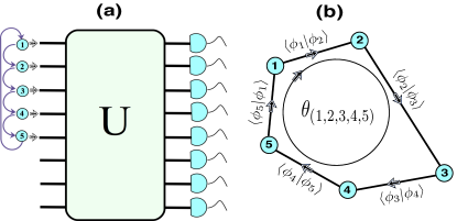
Figure 1: (a) $N$ identical particles are impinging on a multiport with a unitary matrix $U$. The circular arrows illustrate the $N$-particle cycle $(1,2,3,\ldots,N)$ responsible for the circle-dance interference with deterministically distinguishable particles $\alpha$ and $\beta$ for $\beta\neq\alpha\pm 1$ (mod $N$). (b) A weighted directed graph representation of particle distinguishability in panel (a) in the case of pure internal states $|\phi_{k}\rangle$, $k=1,\ldots,N$, where each particle is a vertex and a directed edge $k\to l$ has the complex weight $w(k,l)\equiv-\ln(\langle\phi_{l}|\phi_{k}\rangle)=d_{kl}+i\theta_{kl}$, where $d_{kl}$ serves as the distance between the vertices (here $d_{kl}=\infty$ is indicated by the absence of such an edge) and $\theta_{kl}$ is the phase in the direction $k\to l$. Only two $(R\geq 3)$-particle cycles on a finite path – $1\to 2\to\ldots\to 5\to 1$ and its inverse – contribute to output probability in panel (a), therefore the latter depends on a single collective (five-particle) phase along the edges $\theta_{(1,2,3,4,5)}=\theta_{12}+\theta_{23}+\theta_{34}+\theta_{45}+\theta_{51}$ (see the text).

The internal states define identical particle distinguishability which affects their interference on a linear multiport. For example, in the HOM experiment HOM the main source of photon distinguishability was the arrival time which was recorded to relate it to the dip in the coincidence counting. One can characterize the state of partial distinguishability of identical particles by the degree of possible internal state discrimination. We are mainly interested in the probability of an output configuration $\mathbf{m}$ without account of the internal states (i.e., when the internal states are not resolved by the particle counting detectors or simply ignored) which is mathematically expressed by summation over the probabilities with resolved internal states . The relation between discrimination of the internal states and its effect on multiparticle interference will be briefly considered in section IV (particle counting with discrimination of the internal states is also analyzed to the necessary detail in appendix A). Single photons on an optical multiport, as in Refs. KLM ; E1 ; E2 ; E3 ; E4 ; Metcalf ; ULO ; RWPh , are the main application of the theory. To some extent, the internal state discrimination is routinely done with single photons (e.g., detection of the time of arrival serves as the partial state discrimination).

We will use the fact PartDist that just one complex-valued function on the symmetric group $\mathcal{S}_{N}$ for $N$ particles accounts for the effect of partial distinguishability, if one ignores the information on the internal states at a multiport output (this function can be though of as a generalization of Mandel’s interference visibility $\&$ distinguishability parameter HOM ; Mandel1991 for $N\geq 3$ photons; for full discussion the reader should consult Ref. PartDist ). The exact form of probability of an output configuration $\mathbf{m}$ for interfering identical particles on a linear multiport was studied before PartDist ; BB (for completeness, we also provide brief derivation in appendix A). For independent particles in internal states $\rho^{(1)},\ldots,\rho^{(N)}$ impinging on the input ports $\mathbf{k}=(1,\ldots,N)$ of a unitary multiport $U$, the probability to detect a configuration $\mathbf{m}=(m_{1},\ldots,m_{M})$ in the output ports reads PartDist ; BB

$$p_{N}(\mathbf{l}|\mathbf{k})=\frac{1}{\mathbf{m}!}\sum_{\tau,\sigma\in\mathcal{S}_{N}}J(\tau^{-1}\sigma)\prod_{k=1}^{N}U^{*}_{k,l_{\tau(k)}}U_{k,l_{\sigma(k)}},$$ (1)

where $\mathbf{m}\equiv m_{1}!\ldots m_{M}!$ and the $J$-function accounts for particle distinguishability. In our case it factorizes PartDist according to the disjoint cycle decomposition (see, for instance, Ref. Stanley ) of its argument. Denoting by $cyc(\sigma)$ the set of disjoint cycles of a permutation $\sigma$, we get

$$J(\sigma) = \prod_{\nu\in cyc(\sigma)}g(\nu),$$

$$g(\nu) \equiv (\pm 1)^{|\nu|-1}\mathrm{Tr}\bigl{(}\rho^{(k_{|\nu|})}\rho^{(k_{|\nu|-1})}\ldots\rho^{(k_{1})}\bigr{)},$$ (2)

where $\nu=(k_{1},\ldots,k_{|\nu|})$, $k_{\alpha}\in\{1,\ldots,N\}$, stands for the cycle $k_{1}\to k_{2}\to\ldots\to k_{|\nu|}\to k_{1}$ and $|\nu|$ for its length, the minus sign is due to the signature of a cycle $\mathrm{sgn}(\nu)=(-1)^{|\nu|-1}$ Stanley and applies to fermions.

The specific form of probability in Eqs. (1) and (II) can be understood without a detailed derivation. Indeed, for identical particles the probability $p_{N}(\mathbf{l}|\mathbf{k})$ must be symmetric under permutations of either output ports $\mathbf{l}$ or input ports $\mathbf{k}$ (particles do not have labels). Let us consider a specific $N$-particle transition amplitude on a multiport $\mathcal{A}(\mathbf{k}\to\mathbf{l})\equiv\prod_{k=1}^{N}U_{k,l_{k}}$ with $\mathbf{l}=(l_{1},\ldots,l_{N})$ (i.e., particle $k$ goes to output port $l_{k}$). By the above symmetry of probability, any permutation $\sigma$ of identical particles over the output ports gives another valid transition amplitude contributing to the probability, $\mathcal{A}({\mathbf{k}\to\sigma(\mathbf{l})})=\prod_{k=1}^{N}U_{k,l_{\sigma(k)}}$. The probability, linear in the amplitude and its complex conjugate, is given by the summation over two permutations $\sigma,\tau\in\mathcal{S}_{N}$ in the two amplitudes as in Eq. (1) (with the signature of a permutation in the case of fermions), where there is also a factor equal to the scalar product in $\mathcal{H}^{\otimes N}$ of the internal states, similarly permuted, with the result dependent only on the relative permutation, described by the function $J(\tau^{-1}\sigma)$ in Eq. (1). The disjoint cycles of $\tau^{-1}\sigma$ contribute independent factors, since they permute different particles (the cross-cycle particle distinguishability does not contribute), hence the $J$-function must be in the form of Eq. (II) (which is easily established by considering pure internal states). Finally, by using the arbitrary permutations, we have permuted $m_{l}$ particles in output port $l$ as well, thus have performed the multiple counting of identical terms, hence the factor $\mathbf{m}!$ in the denominator.

Due to the mutual independence of the concept of distinguishability of identical particles and the unitary transformation employed by a multiport, below we will focus on the state of particle distinguishability itself when discussing multiparticle interference on a multiport. Indeed, on a generic multiport, i.e., when none of the matrix elements $U_{kl}$ is zero, all permutations of particles can contribute to the coincidence count output probability and one can observe the discussed examples of multiparticle interference on such a multiport (obviously, an optimization is possible by selecting a particular multiport). We will return to this when discussing a specific example in section III.

From the above discussion, one can derive the physical meaning of the cycles in Eq. (II): to each such cycle can be associated the interference of only the particles involved in the cycle. Below we will frequently use the term “$R$-particle interference” which simply means the contribution from an $R$-cycle in Eq. (II) to the output probability in Eq. (1). Note, however, that a general summation term in Eq. (II) consists of simultaneous and independent interferences of $S_{1},\ldots,S_{d}$ particles according to a partition of $N=S_{1}+\ldots+S_{d}$.

The relative significance of the contribution of $R$-particle interference depends on the $g$-weights of the $R$-cycles in the respective probability. Obviously, there is always two-particle interference, unless the particles have orthogonal internal states, i.e., $\rho^{(k)}\rho^{(l)}=0$ for all $k\neq l$ (distinguishable particles, i.e., the classical case PartDist ). It may happen that some cycles have zero $g$-weight such that there is just two-particle and $N$-particle interference on a multiport. We will say that this case realizes the “genuine $N$-particle interference”, meaning that no $3\leq R\leq N-1$ interference is realized at the same time.

Obviously, no $N$-particle interference contributes to the output probabilities, if one sends a subset of $N$ particles to a multiport. Similarly, no $N$-particle interference contributes to the respective (marginal) output probabilities, when $N$ particles are sent to a multiport input, but at the output the information on some of the particles is lost, or discarded (by binning together the output configurations $\mathbf{m}$ containing a given configuration $\mathbf{m}^{\prime}$ of less than $N$ particles). This is due to the simple fact that the marginal probability of an output configuration for $R$ out of $N$ particles depends only on the $d$-cycles with $d\leq R$. Indeed, one can use the above discussion of Eqs. (1)-(II) to arrive at this conclusion. The probability $p_{N}(\mathbf{l}^{\prime}|\mathbf{k})$ of an output $\mathbf{m}^{\prime}$ with $R<N$ particles $\mathbf{l}^{\prime}=(l^{\prime}_{1},\ldots,l^{\prime}_{R})$ is obtained by partitioning the transition $\mathbf{k}\to\mathbf{l}$ as $(\mathbf{k}^{\prime}\to\mathbf{l}^{\prime},\mathbf{k}^{\prime\prime}\to\mathbf{l}^{\prime\prime})$, summing up over $\mathbf{l}^{\prime\prime}$ (which simply removes the respective matrix elements $U_{kl^{\prime\prime}}$ by the unitarity of $U$) and averaging over all $(R,N-R)$-partitions $(\mathbf{k}^{\prime},\mathbf{k}^{\prime\prime})$ of the input ports, i.e.,

$$p_{N}(\mathbf{l}^{\prime}|\mathbf{k})=\left({N\atop R}\right)^{-1}\sum_{\mathbf{k}^{\prime}\subset\mathbf{k}}p_{R}(\mathbf{l}^{\prime}|\mathbf{k}^{\prime}),$$ (3)

where the summation is over all subsets $\mathbf{k}^{\prime}$ having $R$ indices (for a formal mathematical derivation, see appendix B). In Eq. (3) $p_{R}(\mathbf{l}^{\prime}|\mathbf{k}^{\prime})$ is the probability of $R$ particles at input ports $\mathbf{k}^{\prime}$ to end up at output ports $\mathbf{l}^{\prime\prime}$, given similarly as in Eqs. (1) and (II) but now for $R$ particles, thus it depends only on $d$-cycles with $d\leq R$.

By using the Cauchy-Schwartz inequality for the trace-product of operators, one can prove an important upper bound on the $R$-cycle $g$-weight by the 2-cycle $g$-weights with the same particles (see appendix C)

$$|\mathrm{Tr}(\rho^{(k_{1})}\ldots\rho^{(k_{R})})|^{2}\leq\prod_{\alpha=1}^{R}\mathrm{Tr}(\rho^{(k_{\alpha})}\rho^{(k_{\alpha+1})})$$ (4)

where $\alpha$ is $\textit{mod}\;R$. Up to now, the treatment of identical particle distinguishability was based mainly on combinatorics (permutations), but Eq. (4) suggests a graph interpretation. This, however, requires generalizing the concept of a graph. Let us think of identical particles as vertices, with vertex $i$ being associated with internal state $\rho^{(i)}$ and all the vertices being connected by edges. Our main object of study is a cycle $\nu=(k_{1},\ldots,k_{R})$ on the edges connecting vertices $k_{1},\ldots,k_{R}$ to which we set a complex weight

$$w(\nu) \equiv -\ln\left(\mathrm{Tr}\bigl{\{}\rho^{(k_{|\nu|})}\rho^{(k_{|\nu|-1})}\ldots\rho^{(k_{1})}\bigr{\}}\right)$$ (5)

$$= D_{(k_{1},\ldots,k_{R})}+i\theta_{(k_{1},\ldots,k_{R})},$$

where $D_{(k_{1},\ldots,k_{R})}$ is the path length of the cycle, whereas $\theta_{(k_{1},\ldots,k_{R})}$ (see also fig. 1(b)) we will call the collective $R$-particle phase of the cycle. Note that reversing the cycle orientation changes the sign of the cycle phase (a nonzero cycle phase selects a direction of the path along the cycle). Larger path distance of a cycle means smaller contribution to output probability on a multiport via Eq. (II), whereas Eq. (4) bounds twice the path distance of a higher order cycle by two-vertex cycles on the same edges (a generalization of the usual path addition on a graph). In the case of pure internal states, when the inequality in Eq. (4) becomes equality, one recovers the usual additive distance on a weighted graph and the phases lead to an additional directed graph (see the next section).

The completely indistinguishable particles and the distinguishable (classical) particles have degenerated graphs. The completely indistinguishable particles from independent sources have the same pure internal state (see Refs. PartDist ; BB ) and map to the zero-distance graph with all the vertices coinciding (which makes sense, since the particles are completely indistinguishable). The deterministically distinguishable particles, $\rho^{(i)}\rho^{(j)}=0$, for $i\neq j$, are mapped to a set of vertices lying at infinite distance from each other (the infinite distance between two vertices will be illustrated as absence of the respective edge, as in fig. 1(b)).

III Particles in pure internal states and $N$-particle interference

Consider particles in pure internal states $\rho^{(k)}=|\phi_{k}\rangle\langle\phi_{k}|$, $k=1,\ldots,N$. Let us set $\langle\phi_{k}|\phi_{l}\rangle\equiv r_{kl}e^{i\theta_{kl}}=\exp\{-d_{kl}+i\theta_{kl}\}$, where $r_{kl}=e^{-d_{kl}}$ is the absolute value and $\theta_{kl}=-\theta_{lk}$ is the phase of the inner product. We will call $\theta_{kl}$ the mutual phase of particle $l$ with respect to $k$. For the path distance along an $R$-particle cycle $(k_{1},\ldots,k_{R})$ we now have from Eq. (5)

$$D_{(k_{1},\ldots,k_{R})}=\sum_{\alpha=1}^{R}d_{k_{\alpha},k_{\alpha+1}},$$ (6)

whereas for the collective $R$-particle phase along the cycle

$$\theta_{(k_{1},\ldots,k_{R})}=\theta_{k_{1}k_{2}}+\theta_{k_{2}k_{3}}+\ldots+\theta_{k_{R}k_{1}}$$ (7)

(note the difference between the two concepts of the phase: for $R=2$ the mutual phase $\theta_{kl}$ can be arbitrary, whereas $\theta_{(k,l)}=0$).

We can interpret $d_{kl}$ as the distance between the vertices $k$ and $l$ in a usual distance-weighted graph, whereas the collective phase $\theta_{(k_{1},\ldots,k_{R})}$ (7) leads to a weighted directed graph, see fig. 2, where each directed edge $k\to l$ acquires a real weight $\theta_{kl}$. The two-graph representation is just a single directed graph with complex weights on the edges given by a Hermitian adjacency matrix $w_{kl}\equiv-\ln(\langle\phi_{l}|\phi_{k}\rangle)=d_{kl}+i\theta_{kl}$.

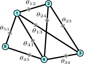
Figure 2: The directed graph for the multiparticle phases, where the mutual phase $\theta_{kl}\equiv\mathrm{arg}(\langle\phi_{k}|\phi_{l}\rangle)$ weights the directed edge $k\to l$. An $(R\geq 3)$-particle collective phase corresponds to a closed oriented path on $R$ vertices. Each closed path on edges has a corresponding multiparticle phase obtained by summation of the mutual phases on the edges passed (with the minus sign, when passing an edge in the inverse direction to the indicated one). The directed paths $1\to 2\to 3\to 1$, $1\to 3\to 4\to 1$ and $1\to 2\to 4\to 1$ allow to express any closed oriented paths on the edges $1,2,3,4$.

Consider the directed graph representation of the collective phases, assuming that none of $r_{kl}$ is zero, i.e., the internal states are only partially distinguishable by the state discrimination Hel ; Chefles . The two-particle collective phase $\theta_{(k,l)}=0$, since the two directed edges $k\to l$ and $l\to k$ cancel each other. For $N=3$ all permutations in $\mathcal{S}_{3}$ are cycles themselves. Since the collective phases of three particleson the same vertices can differ only by a sign (transposition of two particles reverses the path orientation in fig. 2, or $\theta_{(i,j,k)}=\mathrm{sgn}(\sigma)\theta_{(1,2,3)}$, for $\sigma(1,2,3)=(i,j,k)$), consider the 3-cycle $\nu=(1,2,3)$. It has the phase $\theta_{(1,2,3)}\equiv\theta_{12}+\theta_{23}+\theta_{31}$. From the above discussion and section II it is now clear that precisely this phase governs the genuine three-particle interference of Ref. Triad2 , observed experimentally as a variation in the output probability according to this phase (by keeping $r_{kl}$ fixed, while varying the mutual phases $\theta_{kl}$).

We are interested in the setups when there is a collective $N$-particle phase, which cannot be reconstructed with detection of less than $N$ particles, e.g., from any marginal probability. In such a case, we will call such a phase the “genuine $N$-particle phase”. This notion is similar to the triad phase introduced in Ref. Triad2 . From the above discussion and section II, it follows that the two notions coincide for $N=3$. Moreover, as a genuine $(N\geq 4)$-particle phase can serve only the $N$-particle collective phase $\theta_{(k_{1},\ldots,k_{N})}$, when it is independent of all the $R$-particle collective phases $\theta_{(l_{1},\ldots,l_{R})}$ for $3\leq R\leq N-1$. We can now state our first result.

Theorem 1.– Identical particles in pure internal states with no two states being orthogonal do not allow for a genuine $N$-particle phase in an interference experiment on a linear multiport.

Proof.– By the above discussion, the theorem will follow from analysis of the collective phases in Eq. (7). By the linear relations between the mutual and collective phases, the set of all cycles contains as many independent collective phases as there are independent mutual phases $\theta_{kl}$, i.e., exactly $(N-1)(N-2)/2$ phases. Indeed, since the mutual phases $\theta_{kl}$ are defined up to the global phase of a state, exactly $N-1$ of them can be preset to given values by employing the global phase transformation $|\phi_{k}\rangle\to e^{-i\theta_{k}}|\phi_{k}\rangle$ resulting in a phase shift $\theta_{kl}\to\theta_{kl}+\theta_{k}-\theta_{l}$. We can now state the following lemma, which implies theorem 1.

Lemma 1.– For $N$ particles in non-orthogonal pure internal states there are $(N-1)(N-2)/2$ independent triad phases, e.g., $\theta_{(1,k,l)}$ for $2\leq k<l\leq N$. Therefore, all $R$-particle phases, $3\leq R\leq N$, are linear combinations of the triad phases.

Proof.– Let us start with $N=4$ particles, which corresponds to the fully-connected subgraph on the vertices $1,2,3,4$ in fig 2. In this case, we have eight different $3$-cycles, i.e., closed oriented paths on three edges, divided into two groups of four phases, $\theta_{(1,2,3)}$, $\theta_{(1,3,4)}$, $\theta_{(1,2,4)}$, and $\theta_{(2,3,4)}$ and the sign-inverted of these (obtained by transposition of two particles in a cycle). Moreover, we have

$$\theta_{(2,3,4)}=\theta_{(1,2,3)}+\theta_{(1,3,4)}-\theta_{(1,2,4)}.$$ (8)

We need to show that we can express three independent mutual phases as functions of the triad phases $\theta_{(1,2,3)}$, $\theta_{(1,3,4)}$ and $\theta_{(1,2,4)}$. Selecting the mutual phases $\theta_{12}$, $\theta_{23}$, and $\theta_{34}$ as the basis (while setting the rest mutual phases to zero, by using the arbitrariness of the global phase of an internal state) we obtain

$$\theta_{12}=\theta_{(1,2,4)},\;\theta_{23}=\theta_{(1,2,3)}-\theta_{(1,2,4)},\;\theta_{34}=\theta_{(1,3,4)}.$$ (9)

Thus all $R$-particle phases are expressed through the phases $\theta_{(1,2,3)}$, $\theta_{(1,3,4)}$ and $\theta_{(1,2,4)}$, which concludes the proof for $N=4$.

Consider now $N>4$ particles (it is enough to consider just five particles, as in fig. 2). We have to show that the set of phases $\theta_{(1,k,l)}$ is the basis for all possible triad phases. For any triad phase $\theta_{(i,k,l)}$, in the graph representation the corresponding oriented path lies within the complete subgraph on the vertices $1,i,k,l$, which returns us to $N\leq 4$ particles $1,i,k,l$, i.e., to the case considered above. Q.E.D.

In section II we have introduced the notion of the genuine $N$-particle interference and in this section the notion of the genuine $N$-particle phase. Theorem 1 relates the two notions for pure internal states, by stating, in other words, that the genuine $N$-particle phase could be found only in a genuine $N$-particle interference, i.e., when the $R$-particle interferences are forbidden for all $3\leq R\leq N-1$. (We do not know if this relation extends to mixed internal states, since the collective phase of a higher-order cycle in Eq. (5) has no simple linear dependence on the collective phases of lower-order cycles on the same edges.)

III.1 Genuine $N$-particle phase and distinguishability

Theorem 1 states that a genuine $(N\geq 4)$-particles phase may appear only if some particles have orthogonal internal states, i.e., when they behave as distinguishable classical particles with respect to each other, since their internal states can be deterministically discriminated. The deterministic distinguishability prevents quantum interference with two particles HOM ; Mandel1991 . For $N=3$, removing one edge prevents existence of the $3$-cycles and therefore a three-particle interference. On the other hand, the genuine $(N\geq 4)$-particle interference is possible when the respective graph consists of just one cycle, see fig. 1(b), which would prevent $R$-particle interference for $3\leq R\leq N-1$ simply by the absence of an edge. Such an interference would differ conceptually from both the three-particle interference observed in Ref. Triad2 and from the genuine $N$-particle interference from the fully-entangled $N$-particle state GHSZ ; MInt reported in Ref. Triad1 with three photons (by requiring the deterministic distinguishability of particles).

We must find conditions on the internal states of particles that allow for a variable $N$-particle phase (7) while the corresponding graph consists of a single cycle. A given set of parameters $\{r_{kl}\geq 0,0\leq\theta_{kl}<2\pi;1\leq k<l\leq N\}$ comes from the inner products of $N$ vectors $|\phi_{k}\rangle$, $k=1,\ldots,N$, i.e., satisfies $\langle\phi_{k}|\phi_{l}\rangle=r_{kl}e^{i\theta_{kl}}$, if and only if the respective matrix $H_{kl}\equiv r_{kl}e^{i\theta_{kl}}$ (with $H_{kk}=1$) is positive semidefinite Hermitian matrix. The set of conditions $\sum_{l=1}^{N}(1-\delta_{kl})|H_{kl}|=\sum_{l=1}^{N}(1-\delta_{kl})r_{kl}\leq 1$ for $k=1,\ldots,N$ (here $\delta_{kl}$ is the Kronecker delta) is sufficient for $H$ to be such a matrix, since the eigenvalues $\lambda_{1},\ldots,\lambda_{N}$ of $H$ are bounded as follows (known as the Gershgorin circle theorem Gersh )

$$|\lambda_{k}-1|\leq\sum_{l=1}^{N}(1-\delta_{kl})r_{kl}\leq 1$$ (10)

and therefore are all non-negative. Note that the mutual phases $\theta_{kl}$ remain free parameters. We can now formulate our second result.

Theorem 2.– Identical particles in linearly independent internal states $|\phi_{1}\rangle,\ldots,|\phi_{N}\rangle$, where each state being orthogonal to all others except two,

$$\langle\phi_{k}|\phi_{k\pm 1}\rangle\neq 0,\quad\langle\phi_{k}|\phi_{l}\rangle=0,\quad l\neq k\pm 1\quad mod\;N,\quad$$ (11)

can realize the genuine $N$-particle interference on a multiport, governed by a genuine collective $N$-particle phase Eq. (7) due to the permutation cycle $1\to 2\to\ldots\to N\to 1$ and its inverse (independent from the two-particle interference parameters), whereas there is no $R$-particle interference for $3\leq R\leq N-1$.

Proof.– From the above discussion it it clear that theorem 2 follows if there are the state vectors with the inner products as in Eq. (11) and free mutual phases (thus allowing for a free $N$-particle collective phase). By Gershgorin’s circle theorem (10), such state vectors do exist under the condition that $|\langle\phi_{k}|\phi_{k-1}\rangle|+|\langle\phi_{k}|\phi_{k+1}\rangle|\leq 1$, for $k=1,\ldots,N$ (mod $N$). Q.E.D.

Due to the graphical representation by a polygon with the particles as the vertices and no internal edges, see fig. 1(b), such single-cycle $N$-particle interference can be termed the “circle-dance interference”.

Let us further discuss an explicit example of the circle-dance interference with $N=4$ particles and how to detect the respective four-particle collective phase in an experiment. First, we construct the required vectors. One can always find an orthonormal basis $(|e_{1}\rangle,|e_{2}\rangle,|e_{3}\rangle,|e_{4}\rangle)$ such that the matrix $\Phi_{kl}\equiv\langle e_{k}|\phi_{l}\rangle$ reads 

$$\!\!\!\!\Phi=\left(\begin{array}[]{cccc}1&0&0&0\\ r_{12}e^{i\theta_{12}}&\sqrt{1-r^{2}_{12}}&0&0\\ 0&\frac{r_{23}}{\sqrt{1-r^{2}_{12}}}e^{i\theta_{23}}&\frac{\sqrt{1-r^{2}_{12}-r^{2}_{23}}}{\sqrt{1-r^{2}_{12}}}&0\\ r_{14}e^{i\theta_{14}}&-\frac{r_{12}r_{14}}{\sqrt{1-r^{2}_{12}}}e^{i(\theta_{14}-\theta_{12})}&\Phi_{34}&\Phi_{44}\end{array}\right),$$ (16)

$$\!\!\!\Phi_{34}=\frac{r_{34}(1-r^{2}_{12})e^{i\theta_{34}}+r_{12}r_{23}r_{14}e^{i(\theta_{14}-\theta_{12}-\theta_{23})}}{\left[(1-r^{2}_{12})(1-r^{2}_{12}-r^{2}_{23})\right]^{\frac{1}{2}}},$$

$$\!\!\!\Phi_{44}=\left(\frac{1-r^{2}_{12}-r^{2}_{14}}{1-r^{2}_{12}}-|\Phi_{34}|^{2}\right)^{\frac{1}{2}},$$ (17)

where we use $\Phi_{kk}$ to satisfy the normalization condition (set to be real by the freedom of the global phase of a quantum state) and the rest of the row elements to satisfy the cross-state inner products. Obviously, $r_{k,k+1}$ satisfy certain conditions for the above construction to make sense (to satisfy the normalization of the state vectors the expressions in the square roots must be positive). While the set of four conditions $r_{k,k-1}+r_{k,k+1}\leq 1$ (obtained from Gershgorin’s circle theorem (10)) is sufficient, an explicit analysis in this case shows that $\sum_{k=1}^{4}r^{2}_{k,k+1}\leq 1$ is also sufficient (see appendix D). For equal values of $r_{k,k+1}\equiv r$ the two conditions coincide, giving $r\leq 1/2$.

Whereas the three-particle interference is not possible with the states in Eq. (17), there is the four-particle interference due to the cycle $\nu_{4}=(1,2,3,4)$ with the $g$-weight

$$g(\nu_{4})=\pm\prod_{k=1}^{4}\langle\phi_{k}|\phi_{k+1}\rangle=\pm\exp\{-D_{(1,2,3,4)}+i\theta_{(1,2,3,4)}\}.$$ (18)

Besides the deterministic distinguishability of not-the-neighbor particles on the cycle $\nu_{4}=(1,2,3,4)$ the circle-dance interference requires the state-vectors to remain linearly independent (similar as in three-particle case Triad2 ), i.e., unambiguously distinguishable Chefles . Indeed, one can verify that imposing linear dependence of the state vectors $|\phi_{k}\rangle$ (specifically in the case of Eq. (17), by setting $\Phi_{44}=0$) will result in a condition for the mutual phases (making them functions of $r_{k,k+1}$).

We have stated above that any generic multiport can realize the circle-dance interference, i.e., any multiport with no matrix element being zero. Let us consider, as an example, single photons in the symmetric four-port of Ref. ZZH corresponding to the diamond-shaped arrangement of four balanced beamsplitters with one phase plate $\varphi$ inserted into one of the internal paths,

$$U=\frac{1}{2}\left(\begin{array}[]{ccrc}\;e^{i\varphi}&\;e^{i\varphi}&1&1\\ -e^{i\varphi}&-e^{i\varphi}&1&1\\ -1&\;\,1&-1&1\\ \;\,1&-1&-1&1\end{array}\right).$$ (19)

In general, there are $\frac{N!}{R(N-R)!}$ different $R$-cycles with $N$ particles Stanley . The symmetric group $\mathcal{S}_{4}$ contains six 2-cycles, eight 3-cycles, and six 4-cycles, therefore, there are three permutations which are not cycles themselves, but products of disjoint 2-cycles. Since only the neighbor particles in the cyclic order $(1,2,3,4)$ are connected by the edges in the corresponding graph representation, fig. 1(b), only the following eight permutations, besides the trivial $I$, contribute to the probability (divided into groups according to their cycle structure):

$$C_{2}:\;(1,2),\,(2,3),\,(3,4),\,(1,4);$$

$$C_{2\times 2}:\;(1,2)(3,4),\,(1,4)(2,3);$$

$$C_{4}:\;(1,2,3,4),\,(4,3,2,1).$$ (20)

We can rearrange the summation in the probability formula in Eqs. (1) and (II) to represent it as follows

$$p_{N}(\mathbf{l}|\mathbf{k})=\frac{1}{\mathbf{m}!}\sum_{\sigma\in\mathcal{S}_{N}}\mathrm{per}(\mathcal{U}^{*}(I)\circ\mathcal{U}(\sigma))\prod_{\nu\in cyc(\sigma)}g(\nu)$$ (21)

where the symbol “$\circ$” denotes the Hadamard (by-element) product of matrices, $\mathcal{U}_{\alpha,\beta}(\sigma)\equiv U_{k_{\sigma(\alpha)},l_{\beta}}$, and

$$\mathrm{per}(A)=\sum_{\sigma\in\mathcal{S}_{N}}\prod_{k=1}^{N}A_{k,\sigma(k)}.$$ (22)

For $N=4$ photons on the symmetric multiport of Eq. (19) with any of the phase values $\varphi\in\{0,\pi,\pm\pi/2\}$ and the coincidence detection, $\mathbf{l}=\mathbf{k}=(1,2,3,4)$, for the cycles given in Eq. (III.1) we get

$$\mathrm{per}(\mathcal{U}^{*}(I)\circ\,\mathcal{U}(\sigma))=\left\{\begin{array}[]{cc}{3}/{32},&\sigma\in\{I,\,C_{2\times 2}\},\\ -{1}/{32},&\sigma\in\{C_{2},\,C_{4}\}.\end{array}\right.$$ (23)

Using that (for bosons) $g(I)=1$, $g(k,k+1)=r^{2}_{k,k+1}$, $g(1,2,3,4)$ from Eq. (18), and that $g(4,3,2,1)=g^{*}(1,2,3,4)$, we obtain from Eqs. (21) and (23) the probability for the coincidence count as follows

$$p_{4}(\mathbf{k}|\mathbf{k})=\frac{1}{32}\Bigl{\{}3\left(1+r^{2}_{12}r^{2}_{34}+r^{2}_{14}r^{2}_{23}\right)$$

$$\quad-\sum_{k=1}^{4}r^{2}_{k,k+1}-2\prod_{k=1}^{4}r_{k,k+1}\cos\theta_{(1,2,3,4)}\Bigr{\}}.$$ (24)

(For fermions, the only change in formula (III.1) is in the sign at the last two terms, due to the minus sign at $g(k,k+1)$ and $g(1,2,3,4)$.)

Finally, we note that the circle-dance interference is possible also with identical particles in mixed internal states. Indeed, if $\mathrm{Tr}(\rho^{(k)}\rho^{(l)})=0$ for $l\neq k\pm 1$, then by Eq. (4) any cycle $\nu$ passing the edge $kl$ has zero $g$-weight, which prevents any $R$-particle interference with $3\leq R\leq N-1$.

III.2 Four-particle circle-dance interference with single photons having Gaussian spectral profiles

Let us analyze in more detail the case of single photons having Gaussian spectral shapes and different polarizations. We consider each photon in a pure state $|\Phi_{k}\rangle=|\varphi_{k}\rangle|P_{k}\rangle$, where $|P_{k}\rangle=\alpha_{k}|v\rangle+\beta_{k}|h\rangle$, with $|v\rangle$ and $|h\rangle$ being the polarization basis, $|\alpha_{k}|^{2}+|\beta_{k}|^{2}=1$, and (in the frequency basis $|\omega\rangle$)

$$|\varphi_{k}\rangle=\int d\omega\varphi_{k}(\omega)|\omega\rangle,$$ (25)

with

$$\varphi_{k}(\omega)=\left(\frac{1}{\sqrt{\pi}\Delta_{k}}\right)^{1/2}\exp{\left(-\frac{(\omega-\omega_{0k})^{2}}{2\Delta_{k}^{2}}-i\tau_{k}(\omega-\omega_{0k})\right)}.$$ (26)

Here we use the polarization state $|P_{k}\rangle$ to satisfy the necessary orthogonality conditions of theorem 2, thus we introduce an angle $\chi$ and set

$$|P_{1}\rangle=|v\rangle,\quad|P_{2}\rangle=\cos{\chi}|v\rangle+\sin{\chi}|h\rangle,$$

$$|P_{3}\rangle=|h\rangle,\quad|P_{4}\rangle=\sin{\chi}|v\rangle-\cos{\chi}|h\rangle.$$ (27)

We also have

$$\langle\varphi_{k}|\varphi_{j}\rangle=\sqrt{\frac{2\Delta_{k}\Delta_{j}}{\Delta_{k}^{2}+\Delta_{j}^{2}}}\hskip 2.84526pte^{-\eta_{kj}+i\xi_{kj}},$$ (28)

with

$$\eta_{kj} = \frac{1}{2}\left(\frac{\Delta_{k}^{2}\Delta_{j}^{2}}{\Delta_{k}^{2}+\Delta_{j}^{2}}\right)\left[(\tau_{k}-\tau_{j})^{2}-\left(\frac{\omega_{0k}}{\Delta_{k}^{2}}+\frac{\omega_{0j}}{\Delta_{j}^{2}}\right)^{2}\right]$$

$$+ \frac{1}{2}\left(\frac{\omega_{0k}^{2}}{\Delta_{k}^{2}}+\frac{\omega_{0j}^{2}}{\Delta_{j}^{2}}\right),$$

$$\xi_{kj} = \left(\frac{\Delta_{k}^{2}\Delta_{j}^{2}}{\Delta_{k}^{2}+\Delta_{j}^{2}}\right)\left(\frac{\omega_{0k}}{\Delta_{k}^{2}}+\frac{\omega_{0j}}{\Delta_{j}^{2}}\right)(\tau_{j}-\tau_{k})$$ (29)

$$+ (\tau_{k}\omega_{0k}-\tau_{j}\omega_{0j}).$$

From the definition $\langle\Phi_{k}|\Phi_{j}\rangle=r_{kj}e^{i\theta_{kj}}$, we get

$$r_{12} = \cos{\chi}\sqrt{\frac{2\Delta_{1}\Delta_{2}}{\Delta^{2}_{1}+\Delta^{2}_{2}}}e^{\eta_{12}},\quad\theta_{12}=\xi_{12},$$

$$r_{23} = \sin{\chi}\sqrt{\frac{2\Delta_{2}\Delta_{3}}{\Delta^{2}_{2}+\Delta^{2}_{3}}}e^{\eta_{23}},\quad\theta_{23}=\xi_{23},$$

$$r_{34} = \cos{\chi}\sqrt{\frac{2\Delta_{3}\Delta_{4}}{\Delta^{2}_{3}+\Delta^{2}_{4}}}e^{\eta_{34}},\quad\theta_{34}=\pi+\xi_{34},$$

$$r_{41} = \sin{\chi}\sqrt{\frac{2\Delta_{4}\Delta_{1}}{\Delta^{2}_{4}+\Delta^{2}_{1}}}e^{\eta_{14}},\quad\theta_{41}=\xi_{41}.$$ (30)

For $\Delta_{k}\neq\Delta_{l}$ the analysis becomes quite involved, thus we consider below all spectral width being the same, $\Delta_{k}=\Delta$. We have in this case

$$\eta_{k,k+1}=\frac{(\omega_{0k}-\omega_{0,k+1})^{2}}{4\Delta^{2}}+\frac{\Delta^{2}}{4}(\tau_{k}-\tau_{k+1})^{2}$$ (31)

and

$$\xi_{k,k+1}=\frac{1}{2}(\tau_{k}+\tau_{k+1})(\omega_{0k}-\omega_{0,k+1}).$$ (32)

From Eqs. (7), (30) and (32) the four-particle collective phase becomes

$$\theta_{(1,2,3,4)} = \pi+\frac{1}{2}\Bigl{[}(\omega_{04}-\omega_{02})(\tau_{1}-\tau_{3})$$ (33)

$$+(\omega_{03}-\omega_{01})(\tau_{4}-\tau_{2})\Bigr{]}.$$

Eqs. (31) and (33) involve the differences of four frequencies and four arrival times, hence they contain only six real parameters additionally to the polarization angle $\chi$ of Eq. (27). One can therefore arrange for the two-particle interference parameters $r_{kj}$ (30) to remain fixed, which takes up only four free parameters from the total seven, thus leaving the four-particle collective phase (33) to vary on a three-parameter manifold. Therefore, the four-particle circle dance interference can be observed with the photons in Gaussian spectral profiles when one can arrange for variable central frequencies of the spectral states and the photon arrival times.

The above example serves only for illustration, since it may be experimentally challenging. There are other possible ways to arrange for the circle dance interference, one such way is reported elsewhere Cleo .

IV The circle-dance interference and multiparticle correlations

What is the reason behind the fact that the collective phase of the circle-dance interference of $N$ particles cannot be detected in an experiment with less than $N$ particles (irrespectively if some particles are simply not sent to a multiport, there are particle losses, or one bins together the output configurations containing a given configuration with less than $N$ particles)? Here we show that such a phase is a signature of the genuine $N$th-order quantum correlations between them, i.e., the correlations not reducible to the lower-order ones.

We will use the fact that detection of $R$ photons is related to the $R$-th order correlation function Glauber of the quantum field. This relation extends also to our case, when the internal states of identical particles are not resolved (which corresponds to a generalized measurement, mathematically expressed by summing up the probabilities with the resolved internal states). Therefore, we can adopt as the unnormalized $R$th order correlation function $Q_{R}(\mathbf{l})$ in $R$ output ports $\mathbf{l}^{\prime}=(l_{1},\ldots,l_{R})$ the following expression

$$Q_{R}(\mathbf{l}^{\prime})=\left\langle\sum_{\mathbf{j}}\left(\prod_{\alpha=1}^{R}\hat{b}^{\dagger}_{l_{\alpha},j_{\alpha}}\right)\left(\prod_{\alpha=1}^{R}\hat{b}_{l_{\alpha},j_{\alpha}}\right)\right\rangle,$$ (34)

where we sum over the basis states in $\mathcal{H}^{\otimes R}$, $\hat{b}^{\dagger}_{l,j}$ creates a particle in output port $l$ of a multiport and an internal state $j$, and the average is taken with the input state. For $N$ particles in input $\mathbf{k}$, the corresponding function $Q_{R}(\mathbf{l}^{\prime}|\mathbf{k})$, as the probability $p_{N}(\mathbf{l}^{\prime}|\mathbf{k})$ in Eq. (3), depends only on the $d$-cycles with $d\leq R$, since the two are proportional (see appendix E)

$$Q_{R}(\mathbf{l}^{\prime}|\mathbf{k})=\mathbf{m}^{\prime}!\left({N\atop R}\right)p_{N}(\mathbf{l}^{\prime}|\mathbf{k})=\mathbf{m}^{\prime}!\sum_{\mathbf{k}^{\prime}\subset\mathbf{k}}p_{R}(\mathbf{l}^{\prime}|\mathbf{k}^{\prime}).$$ (35)

By Eq. (35) all $Q_{R}(\mathbf{l}^{\prime}|\mathbf{k})$ for $R\leq N-1$ are independent of the $N$-particle collective phase of Eq. (7).

Note that $Q_{R}(\mathbf{l}^{\prime}|\mathbf{k})$ contains both quantum and classical correlations, in the classical case (distinguishable particles in orthogonal internal states) it is proportional to the respective classical probability. The classical correlation function is therefore independent of the collective phases (since particles in the orthogonal internal states do not have collective phases).

Eq. (35) together with the results of the previous sections means that some popular criteria for distinguishing quantum and classical behavior of identical particles in unitary linear multiports as in Ref. Wal and the recently introduced nonclassicality criteria for interference in multiport interferomentry Nonclass , based on the second-order correlation, will not be able to detect quantum $R$-particle phases, for all $R\geq 3$, since they are related to higher than the second-order correlations. Therefore, though such criteria may detect some quantum behavior at a multiport output, they are far from being sufficient for this purpose.

IV.1 Discrimination of internal states and multiparticle interference

Up to now we have assumed that particle detection at the output of a linear multiport does not resolve the internal states of particles. Let us now discuss an internal state resolving detection (see appendix A for the mathematical details of state resolving detection).

If a detector resolves the internal state of at least one particle, the $N$-particle interference does not contribute to the respective probability. Let us illustrate this using the circle-dance $N$-particle interference with identical particles in pure internal states, which requires the internal states to be linearly independent, i.e., unambiguously distinguishable by the scheme of Ref. Chefles . The unambiguous discrimination scheme of Ref. Chefles runs as follows. The state $|\phi_{k}\rangle$ is identified with some probability $p_{k}$, the corresponding measurement operator being $\Pi_{k}=p_{k}|\phi^{(\perp)}_{k}\rangle\langle\phi^{(\perp)}_{k}|$, where $\langle\phi^{(\perp)}_{k}|\phi_{l}\rangle=\delta_{kl}$, whereas an inconclusive result corresponds to $\Pi_{0}=\openone-\sum_{k=1}^{N}\Pi_{k}$. In the graph representation, see fig. 1(b), even a single such an internal state detection with a conclusive result implies that vertex $k$ has no edges (since a particular input particle is detected at an output port, it does not participate in the permutations of particles in the quantum amplitudes, as discussed in section II). Broken edge in the cycle of fig. 1(b) means that the $N$-particle interference is not observed (neither the $(R\geq 3)$-particle interference in this case). The inconclusive result, on the other hand, does not affect the terms in the probability coming from the $(R\geq 2)$-cycles, due to $\langle\phi_{k}|\Pi_{0}|\phi_{l}\rangle=\langle\phi_{k}|\phi_{l}\rangle$ for $k\neq l$, (the edges of the respective graph retain their weights), while simultaneously attenuating the permutations with fixed points, since for each fixed point we have in this case $\langle\phi_{k}|\Pi_{0}|\phi_{k}\rangle=1-p_{k}$, instead of $g(k)=1$ in the state non-resolving detection. Since in the case of the circle-dance interference there are just the two-cycles $(k,k+1)$ and the full $N$-cycle, such a generalized detection attenuates the two-particle interference (the permutations having fixed points). Thus the unambiguous state discrimination would separate the outcomes with either destructed or relatively enhanced circle-dance interference.

The above discussion indicates that the internal state discrimination, even if partial (e.g., the resolution of the arrival times of single photons), can strongly affect the multiparticle interference. Whether one is technically able to perform generalized measurements on the internal states of identical particles, as required in the above unambiguous state discrimination scheme, is another problem that depends on the particular physical setup, the type of identical particles used and the degrees of freedom that serve as the Hilbert space of the internal states.

V Conclusion

We have provided a general framework which allows to study the complex relation between particle distinguishability and higher-order interference effects of independent identical bosons or fermions on a linear multiport. We have introduced the collective geometric phases of identical particles, which govern multiparticle interferences, and related them to the higher-order quantum correlations acquired between independent particles via propagation in a linear multiport. We also have opened the discussion on exact relation between the state-discrimination distinguishability and the distinguishability in the multiparticle interference, by showing that the genuine $N$-particle interference for $N\geq 4$ independent particles in pure internal states requires each particle to be unambiguously distinguishable from all others and deterministically distinguishable from all but two. We show, for instance, that the unambiguous internal state discrimination is detrimental to the interference. However, the latter gets an enhanced visibility, if the measurement result is inconclusive.

Throughout the work we have seen an interesting connection of the partial distinguishability theory to the theory of weighted graphs. We show, for instance, how the usual concept of a weighted directed graph with $N$ vertices appears in the interference of $N$ identical particles in pure internal states, where the weights are defined by the inner products of the internal states. Though one could also obtain all our results by using only the combinatorics with permutations, this connection by itself is very interesting. Indeed, the weighted graph theory is intimately linked with one of most studied computationally hard problems, namely, the traveling salesman problem TSP . Such a connection and what it has to say about the computational complexity of partially distinguishable identical particles is worth exploring in the future publications.

VI Acknowledgements

V.S. was supported by the National Council for Scientific and Technological Development (CNPq) of Brazil, grant 304129/2015-1, and by the São Paulo Research Foundation (FAPESP), grant 2015/23296-8. M. E. O. was supported by FAPESP, grant number 2017/06774-9.

Appendix A Brief derivation of Eqs. (1) and (II)

Here we provide brief derivation of output probability formula which reduces to Eqs. (1) and (II) for particle counting nonresolving the internal states. We follow Ref. PartDist and the Supplemental Material to Refs. BB ; GL . Below we consider simultaneously bosons and fermions using the fact that the respective probability is identical for the same $J$-function (the internal states for the same $J$-function are obviously not the same).

The general possible mixed state of $N$ partially-distinguishable particles impinging at $\mathbf{k}=(k_{1},\ldots,k_{N})$ input ports of a unitary $M$-port $U$, corresponding to the occupations $\mathbf{n}=(n_{1},\ldots,n_{M})$, can always be cast as follows

$${\rho}(\mathbf{n})=\sum_{i}p_{i}|\Psi_{i}\rangle\langle\Psi_{i}|,\quad|\Psi_{i}\rangle=\frac{1}{\sqrt{\mathbf{n}!}}\sum_{\mathbf{j}}C^{(i)}_{\mathbf{j}}\prod_{\alpha=1}^{N}\hat{a}^{\dagger}_{k_{\alpha},j_{\alpha}}|0\rangle,$$ (36)

where $\hat{a}^{\dagger}_{k,j}$ is the creation operator of a boson (fermion) in port $k$ and an internal basis state $|j\rangle\in\mathcal{H}$, $\mathbf{n}!=n_{1}!\ldots n_{M}!$, $\mathbf{j}=(j_{1},\ldots,j_{N})$, and $p_{i}\geq 0$ with $\sum_{i}p_{i}=1$. The permutation symmetry (anti-symmetry) of the operators for bosons (fermions) allows one to choose the expansion coefficients $C^{(i)}_{\mathbf{j}}$ to be symmetric (anti-symmetric) with respect to the symmetry subgroup $\mathcal{S}_{\mathbf{n}}\equiv\mathcal{S}_{n_{1}}\otimes\ldots\otimes\mathcal{S}_{n_{M}}$ of the symmetric group $\mathcal{S}_{N}$, where $\mathcal{S}_{n_{k}}$ corresponds to the permutations of the internal states of the particles in input port $k$ between themselves. The symmetric (anti-symmetric) coefficients are normalized by $\sum_{\mathbf{j}}|C^{(i)}_{\mathbf{j}}|^{2}=1$.

A linear multiport $U$ performs the unitary transformation $\hat{a}^{\dagger}_{k,j}=\sum_{l=1}^{M}U_{kl}\hat{b}^{\dagger}_{l,j}$. Consider a particle counting at the multiport output capable of not only the particle-number, but also the internal state resolution. First, let us assume that the internal states are resolved by the projective measurement in some orthogonal basis (let it be the same as in Eq. (36)). The probability of the output $(l_{1},j_{1}),\ldots,(l_{N},j_{N})$ in the $b$-basis, with the corresponding particle counts $s_{l,j}\geq 1$, reads

$$p_{N}(\mathbf{l},\mathbf{j}|\mathbf{k})=\mathrm{Tr}({\rho}(\mathbf{n})\mathcal{D}(\mathbf{s})).$$ (37)

where

$$\mathcal{D}(\mathbf{s})=\frac{1}{\mathbf{s}!}\left[\prod_{\alpha=1}^{N}\hat{b}^{\dagger}_{l_{\alpha},j_{\alpha}}\right]|0\rangle\langle 0|\left[\prod_{\alpha=1}^{N}\hat{b}_{l_{\alpha},j_{\alpha}}\right].$$ (38)

Using the following identity

$$\langle 0|\left[\prod_{\alpha=1}^{N}\hat{b}_{l_{\alpha},j_{\alpha}}\right]\left[\prod_{\alpha=1}^{N}\hat{b}^{\dagger}_{l^{\prime}_{\alpha},j^{\prime}_{\alpha}}\right]|0\rangle$$

$$=\sum_{\sigma\in\mathcal{S}_{N}}\varepsilon(\sigma)\prod_{\alpha=1}^{N}\delta_{l^{\prime}_{\alpha},l_{\sigma(\alpha)}}\delta_{j^{\prime}_{\alpha},j_{\sigma(\alpha)}},$$ (39)

with $\varepsilon(\sigma)=1$ for bosons and $\varepsilon(\sigma)=\mathrm{sgn}(\sigma)$ for fermions, one obtains

$$p_{N}(\mathbf{l},\mathbf{j}|\mathbf{k})=\frac{1}{\mathbf{s}!\mathbf{n}!}\sum_{\tau,\sigma\in\mathcal{S}_{N}}J(\mathbf{j};\tau^{-1},\sigma)\prod_{a=1}^{N}U^{*}_{k_{\alpha},l_{\tau(\alpha)}}U_{k_{\alpha},l_{\sigma(\alpha)}},$$ (40)

where the $J$-function reads

$$J(\mathbf{j};\tau,\sigma)=\varepsilon(\sigma\tau)\mathrm{Tr}\left(\Pi_{j_{1}}\otimes\ldots\otimes\Pi_{j_{N}}P_{\sigma}\rho^{(int)}P_{\tau}\right)$$ (41)

with $\Pi_{j}=|j\rangle\langle j|$ and the internal state $\rho^{(int)}$ given as

$$\rho^{(int)}=\sum_{i}p_{i}|\psi_{i}\rangle\langle\psi_{i}|,\quad|\psi_{i}\rangle\equiv\sum_{\mathbf{j}}C^{(i)}_{\mathbf{j}}\prod_{\alpha=1}^{N}{\!}^{\otimes}|j_{\alpha}\rangle.$$ (42)

Note the symmetry property of the $J$-function. The permutation symmetry (anti-symmetry) of the internal state (42) for bosons (fermions), i.e., $P_{\pi}\rho^{(int)}=\rho^{(int)}P_{\pi}=\varepsilon(\pi)\rho^{(int)}$ for any $\pi\in\mathcal{S}_{\mathbf{n}}$, implies that

$$J(\mathbf{j};\tau,\sigma\pi)=J(\mathbf{j};\pi\tau,\sigma)=J(\mathbf{j};\tau,\sigma),\quad\forall\pi\in\mathcal{S}_{\mathbf{n}}.$$ (43)

For independent particles $\rho^{(int)}=\rho^{(1)}\otimes\ldots\otimes\rho^{(N)}$ the expression for the $J$-function in Eq. (41) can be simplified. Using that

$$P^{\dagger}_{\sigma}\left(\prod_{\alpha=1}^{N}\Pi_{\alpha}\right)P_{\sigma}=\prod_{\alpha=1}^{N}\Pi_{\sigma(\alpha)}$$ (44)

we get

$$J=\varepsilon(\sigma\tau)\mathrm{Tr}\left(P^{\dagger}_{\sigma^{-1}\tau}\Pi_{j_{\sigma(1)}}\rho^{(1)}\otimes\ldots\otimes\Pi_{j_{\sigma(N)}}\rho^{(N)}\right)$$

$$=\prod_{\nu}(\pm 1)^{|\nu|-1}\mathrm{Tr}\left(\Pi_{j_{\sigma(\alpha_{1})}}\rho^{(\alpha_{1})}\ldots\Pi_{j_{\sigma(\alpha_{|\nu|})}}\rho^{(\alpha_{|\nu|})}\right),$$

where $\nu=(\alpha_{1},\ldots,\alpha_{|\nu|})$ is from the disjoint cycle decomposition of $\sigma^{-1}\tau$, we have used that $\varepsilon(\nu)=(\pm 1)^{|\nu|-1}$ Stanley and the identity

$$\mathrm{Tr}(P^{\dagger}_{\sigma}A^{(1)}\otimes\ldots\otimes A^{(N)})$$

$$=\prod_{\nu\in cyc(\sigma)}\mathrm{Tr}(A^{(\alpha_{1})}\otimes\ldots\otimes A^{(\alpha_{|\nu|})}).$$ (46)

Though we have considered above the specific projective measurement, $\Pi_{j}=|j\rangle\langle j|$, by the linearity property Eqs. (41)-(A) apply also for arbitrary POVM elements $\Pi_{j}$, where $\sum_{j}\Pi_{j}=\openone$.

For the particle counting not resolving their internal states, which is obtained by summation of the probabilities with all possible $\Pi_{j}$ elements in  Eq. (40) for a fixed set of the output ports $\mathbf{l}=(l_{1},\ldots,l_{N})$, the probability reads

$$p_{N}(\mathbf{l}|\mathbf{k})=\sum_{\mathbf{j}}p_{N}(\mathbf{l},\mathbf{j}|\mathbf{k})$$ (47)

$$=\frac{1}{\mathbf{m}!\mathbf{n}!}\sum_{\tau,\sigma\in\mathcal{S}_{N}}J(\tau^{-1}\sigma)\prod_{a=1}^{N}U^{*}_{k_{\alpha},l_{\tau(\alpha)}}U_{k_{\alpha},l_{\sigma(\alpha)}},$$

with $\mathbf{m}=(m_{1},\ldots,m_{M})$ being the corresponding occupations and

$$J(\sigma)=\varepsilon(\sigma)\mathrm{Tr}\bigl{(}P_{\sigma}\rho^{(int)}\bigr{)}.$$ (48)

For independent particles and single particle per input port, from Eqs. (A), (47) and (48) we obtain Eqs. (1)-(II) of section II.

Appendix B The probability to detect $R$ out of $N$ particles

Here we give a direct mathematical derivation of the probability formula in Eq. (3), in particular, we prove the fact that the marginal probability of detecting $R<N$ particles from $N$ input ones depends only on the cycles with length not exceeding $R$.

First of all, since identical particles bear no labels, we have (see also the note in section II)

$$p_{N}(\sigma(\mathbf{l})|\mathbf{k})=p_{N}(\mathbf{l}|\sigma(\mathbf{k}))=p_{N}(\mathbf{l}|\mathbf{k}),\quad\sigma\in\mathcal{S}_{N},$$ (49)

where $\sigma(\mathbf{l})=(l_{\sigma(1)},\ldots,l_{\sigma(N)})$ (and similar for $\mathbf{k}$). For definiteness, let us assume that $\mathbf{k}$ are ordered, $k_{\alpha}\leq k_{\alpha+1}$.

Consider now a symmetric function in $N$ variables $f(\mathbf{l})$. Denote by $m_{k}$ the number of occurrences of $l_{\alpha}=k$ and set $\mathbf{m}=(m_{1},\ldots,m_{M})$. Partitioning $\mathbf{l}=(\mathbf{l}^{\prime},\mathbf{l}^{\prime\prime})$ such that $\mathbf{l}^{\prime}=(l_{1},\ldots,l_{R})$ (and, correspondingly, $\mathbf{m}=(\mathbf{m}^{\prime},\mathbf{m}^{\prime\prime})$) we get

$$\sum_{\mathbf{m}}f(\mathbf{l})=\sum_{\mathbf{l}}\frac{\mathbf{m}!}{N!}f(\mathbf{l})=\frac{1}{N!}\sum_{\mathbf{l}^{\prime}}\sum_{\mathbf{l}^{\prime\prime}}\mathbf{m}!f(\mathbf{l})$$

$$=\left({N\atop R}\right)^{-1}\sum_{\mathbf{m}^{\prime}}\sum_{\mathbf{m}^{\prime\prime}}\frac{\mathbf{m}!}{\mathbf{m}^{\prime}!\mathbf{m}^{\prime\prime}!}f(\mathbf{l}),$$ (50)

where the summation runs over $|\mathbf{m}|\equiv m_{1}+\ldots m_{M}=N$, $|\mathbf{m}^{\prime}|=R$, and $|\mathbf{m}^{\prime\prime}|=N-R$. Eq. (B) applied to the probability $p_{N}(\mathbf{l}|\mathbf{k})$ supplies the expression for the probability to detect $R$ particles out of $N$, corresponding to occupations $\mathbf{m}^{\prime}$

$$p_{N}(\mathbf{l}^{\prime}|\mathbf{k})\equiv\left({N\atop R}\right)^{-1}\sum_{\mathbf{m}^{\prime\prime}}\frac{\mathbf{m}!}{\mathbf{m}^{\prime}!\mathbf{m}^{\prime\prime}!}p_{N}(\mathbf{l}|\mathbf{k}),$$ (51)

where $\mathbf{l}$ is partitioned as above.

Since the probability $p_{N}(\mathbf{l}|\mathbf{k})$ is symmetric in both $\mathbf{k}$ and $\mathbf{l}$, we can rearrange $\mathbf{l}$ such that $\mathbf{l}^{\prime}=(l_{1},\ldots,l_{R})$. Now we plug the general formula Eq. (47) (in an equivalent form) into Eq. (51):

$$p_{N}(\mathbf{l}^{\prime}|\mathbf{k})=\frac{R!}{N!\mathbf{m}^{\prime}!\mathbf{n}!}\sum_{\sigma_{1,2}\in\mathcal{S}_{N}}J(\sigma_{1}\sigma^{-1}_{2})$$

$$\times\sum_{\mathbf{l}^{\prime\prime}}\prod_{\alpha=1}^{N}U^{*}_{k_{\sigma_{1}(\alpha)},l_{\alpha}}U_{k_{\sigma_{2}(\alpha)},l_{\alpha}}$$

$$=\frac{R!}{N!\mathbf{m}^{\prime}!\mathbf{n}!}\sum_{\sigma_{1,2}\in\mathcal{S}_{N}}J(\sigma_{1}\sigma^{-1}_{2})\left[\prod_{\alpha=1}^{R}U^{*}_{k_{\sigma_{1}(\alpha)},l_{\alpha}}U_{k_{\sigma_{2}(\alpha)},l_{\alpha}}\right]$$

$$\times\prod_{\alpha=R+1}^{N}\delta_{k_{\sigma_{1}(\alpha)},k_{\sigma_{2}(\alpha)}},$$ (52)

where we have used the unitarity of the multiport matrix $U$. Let us decompose the permutations $\sigma_{1,2}$ as follows

$$\sigma_{i}=(\sigma_{i}^{\prime}\otimes\sigma^{\prime\prime}_{i})\tau_{i},\quad\sigma_{i}^{\prime}\in\mathcal{S}_{R},\quad\sigma_{i}^{\prime\prime}\in\mathcal{S}_{N-R},$$ (53)

i.e., we define $\tau_{i}\in\mathcal{S}_{N}/(\mathcal{S}_{R}\mathcal{S}_{N-R})$, the permutation choosing two subsets of $R$ and $N-R$ indices from $1\leq\alpha\leq N$ without changing the proper order of the indices in each subset. Then $\tau_{i}(\mathbf{k})\equiv(k_{\tau_{i}(1)},\ldots,k_{\tau_{i}(N)})=(\mathbf{k}^{\prime(i)},\mathbf{k}^{\prime\prime(i)})$ with $k^{\prime}_{\alpha}\leq k^{\prime}_{\alpha+1}$ and $k^{\prime\prime}_{\alpha}\leq k^{\prime\prime}_{\alpha+1}$ (by our choice of the order of $k_{\alpha}$). We have

$$\prod_{\alpha=R+1}^{N}\delta_{k_{\sigma_{1}(\alpha)},k_{\sigma_{2}(\alpha)}}=\delta_{\mathbf{k}^{\prime(1)},\mathbf{k}^{\prime(2)}}\prod_{\alpha=1}^{N-R}\delta_{k^{\prime\prime}_{\sigma^{\prime\prime}_{1}(\alpha)},k^{\prime\prime}_{\sigma^{\prime\prime}_{2}(\alpha)}}$$

$$\qquad=\delta_{\mathbf{k}^{\prime(1)},\mathbf{k}^{\prime(2)}}\sum_{\pi\in\mathcal{S}_{\mathbf{n}^{\prime\prime}}}\delta_{\sigma^{\prime\prime}_{1}(\sigma^{\prime\prime}_{2})^{-1},\pi}$$ (54)

where $\mathcal{S}_{\mathbf{n}^{\prime\prime}}\equiv\mathcal{S}_{n^{\prime\prime}_{1}}\otimes\ldots\otimes\mathcal{S}_{n^{\prime\prime}_{M}}$ is the symmetry group of the input configuration $\mathbf{k}^{\prime\prime}$ with the occupations $\mathbf{n}^{\prime\prime}$. For $\pi\in\mathcal{S}_{\mathbf{n}}$ and an arbitrary $\sigma\in\mathcal{S}_{N}$ we have from Eq. (43)

$$J(\sigma\pi)=J(\pi\sigma)=J(\sigma).$$ (55)

In our case

$$\sigma_{2}\sigma^{-1}_{1}=\sigma^{\prime}_{2}(\sigma^{\prime}_{1})^{-1}\otimes\pi^{\prime\prime}=(\sigma^{\prime}_{2}(\sigma^{\prime}_{1})^{-1}\otimes I)\pi,$$ (56)

with $\pi\equiv I\otimes\pi^{\prime\prime}\in\mathcal{S}_{\mathbf{n}}$. Now note the following identity, valid for any symmetric function $f(\mathbf{k}^{\prime})$,

$$\sum_{\sigma_{1,2}}\delta_{\mathbf{k}^{\prime(1)},\mathbf{k}^{\prime(2)}}\sum_{\pi\in\mathcal{S}_{\mathbf{n}^{\prime\prime}}}\delta_{\sigma^{\prime\prime}_{1}(\sigma^{\prime\prime}_{2})^{-1},\pi}f(\mathbf{k}^{\prime})$$

$$\qquad=(N-R)!\sum_{\mathbf{k}^{\prime}\subset\mathbf{k}}\frac{\mathbf{n}!}{\mathbf{n}^{\prime}!}f(\mathbf{k}^{\prime}),$$ (57)

where the sum over permutations is reduced to that over values $\mathbf{k}^{\prime}$, we have used that exactly $\frac{\mathbf{n}!}{\mathbf{n}^{\prime}!\mathbf{n}^{\prime\prime}!}$ of $\tau_{2}$ give the same set of values $\mathbf{k}^{\prime(2)}$ as $\mathbf{k}^{\prime(1)}$, the number of permutations $\pi\in\mathcal{S}_{\mathbf{n}^{\prime\prime}}$ and that one $\sigma^{\prime\prime}_{i}\in\mathcal{S}_{N-R}$ can be chosen arbitrary. By using the identity from Eq. (B), the fact that the summation over $\tau_{1}$ is equivalent to that over the ordered subsets $\mathbf{k}^{\prime}\subset\mathbf{k}$ (or over all choices of $R$ particles from $N$), and that there are exactly $\mathbf{n}^{\prime\prime}!$ permutations in $\mathcal{S}_{\mathbf{n}^{\prime\prime}}$, we obtain from Eqs. (B)-(56):

$$p_{N}(\mathbf{l}^{\prime}|\mathbf{k})=\left({N\atop R}\right)^{-1}\sum_{\mathbf{k}^{\prime}\subset\mathbf{k}}p_{R}(\mathbf{l}^{\prime}|\mathbf{k}^{\prime}),$$ (58)

where we have introduced the probability of the particles from input $\mathbf{k}^{\prime}$ to be detected at the output ports $\mathbf{l}^{\prime}$

$$p_{R}(\mathbf{l}^{\prime}|\mathbf{k}^{\prime}) = \frac{1}{\mathbf{m}^{\prime}!\mathbf{n}^{\prime}!}\sum_{\sigma_{1,2}\in\mathcal{S}_{R}}J_{\mathbf{n}^{\prime}}(\sigma_{1}\sigma^{-1}_{2})$$ (59)

$$\times\prod_{\alpha=1}^{R}U^{*}_{k_{\sigma_{1}(\alpha)},l_{\alpha}}U_{k_{\sigma_{2}(\alpha)},l_{\alpha}}.$$

Here $J_{\mathbf{n}^{\prime}}$-function is defined as in Eq. (II) of section II for the internal states of the particles labelled by $\mathbf{k}^{\prime}$.

Since the probability in Eq. (58) is given by averaging the respective probabilities $p_{R}(\mathbf{l}^{\prime}|\mathbf{k}^{\prime})$ with input of $R$ particles (selected arbitrarily from $N$), therefore it depends only on the cycles of length $d\leq R$.

Appendix C Bound on the $g$-weight

The bound is valid for arbitrary positive semi-definite Hermitian operators $A_{1},\ldots,A_{n}$, i.e.,

$$|\mathrm{Tr}(A_{1}\ldots A_{n})|^{2}\leq\prod_{k=1}^{n}\mathrm{Tr}(A_{k}A_{k+1}),$$ (60)

where $k$ is $\textit{mod}\;n$. Note that $\mathrm{Tr}(A_{k}A_{k+1})$ is real and positive. Eq. (60) can be proven by using the Cauchy-Schwartz inequality for the Hilbert-Schmidt (a.k.a. Frobenius) norm, i.e., for any two operators $A$ and $B$ having finite Frobenius norm

$$|\mathrm{Tr}(A^{\dagger}B)|\leq\sqrt{\mathrm{Tr}(A^{\dagger}A)}\sqrt{\mathrm{Tr}(B^{\dagger}B)}\equiv||A||\cdot||B||.$$ (61)

Now let us introduce the positive semi-definite Hermitian operator $A^{\frac{1}{2}}_{k}$, i.e., $A^{\frac{1}{2}}_{k}A^{\frac{1}{2}}_{k}=A_{k}$. Rearranging the factors by placing one $A^{\frac{1}{2}}_{1}$ to the right, we have

$$|\mathrm{Tr}(A_{1}\ldots A_{n})|=|\mathrm{Tr}\{(A^{\frac{1}{2}}_{1}A^{\frac{1}{2}}_{2})(A^{\frac{1}{2}}_{2}A^{\frac{1}{2}}_{3})\ldots(A^{\frac{1}{2}}_{n}A^{\frac{1}{2}}_{1})\}|$$

$$\leq||A^{\frac{1}{2}}_{1}A^{\frac{1}{2}}_{2}||\ldots||A^{\frac{1}{2}}_{n}A^{\frac{1}{2}}_{1}||=\prod_{k=1}^{n}\sqrt{\mathrm{Tr}(A_{k}A_{k+1})},$$ (62)

where we have used Eq. (61), the submultiplicativity of the Frobenius norm $||AB||\leq||A||\cdot||B||$ and the effective commutativity when evaluating the trace of a product of two operators.

Appendix D Roots of the matrix $H$ for $N=4$

In this case we have for the characteristic equation for $H_{kl}=\langle\phi_{k}|\phi_{l}\rangle=r_{kl}e^{i\theta_{kl}}$:

$$\mathrm{det}(H-\lambda I)=(\lambda-1)^{4}-(\lambda-1)^{2}a_{2}+a_{0},$$ (63)

with $a_{2}=r^{2}_{12}+r^{2}_{23}+r^{2}_{34}+r^{2}_{14}$ and

$$a_{0}=|r_{12}r_{34}e^{i(\theta_{12}+\theta_{34})}-r_{14}r_{23}e^{i(\theta_{14}+\theta_{32})}|^{2}.$$ (64)

We need to require that $\lambda\geq 0$ for the matrix $H$ to be positive semidefinite Hermitian matrix. For the roots we get

$$(\lambda-1)^{2}=\frac{1}{2}\left(a_{2}\pm\sqrt{a_{2}-4a_{0}}\,\right).$$ (65)

Now, using that $a^{2}_{2}\geq 4a_{0}$ (the matrix $H$ is Hermitian, therefore the roots are real) we get from Eq. (65) that $a_{2}\leq 1$ is a sufficient condition for the matrix $H$ to be positive semidefinite.

Appendix E The expression for the correlation function

Note that following expression for the projector on the symmetric (anti-symmetric) subspace of $N-R$ particles (when one discards the information on the internal states in $\mathcal{H}$)

$$S_{N-R}=\sum_{\mathbf{m}^{\prime\prime}}\frac{1}{\mathbf{m}^{\prime\prime}!}\sum_{\mathbf{j}}\left(\prod_{\alpha=1}^{N-R}\hat{b}^{\dagger}_{l^{\prime\prime}_{\alpha},j_{\alpha}}\right)|0\rangle\langle 0|\left(\prod_{\alpha=1}^{N-R}\hat{b}_{l^{\prime\prime}_{\alpha},j_{\alpha}}\right)$$ (66)

where $\mathbf{m}^{\prime\prime}$ is the occupations of $N-R$ particles in the output ports $\mathbf{l}^{\prime\prime}=(l^{\prime\prime}_{1},\ldots,l^{\prime\prime}_{N-R})$ (in the partition $\mathbf{l}=(\mathbf{l}^{\prime},\mathbf{l}^{\prime\prime})$). Using the fact that the correlation function is computed for an $N$-particle state $\rho(\mathbf{n})$ (symmetric or anti-symmetric under particle permutations, respectively, for bosons and fermions) by inserting the projector of Eq. (66) into the expression in Eq. (34) we get

$$Q_{R}(\mathbf{l}^{\prime}|\mathbf{k})=\left\langle\sum_{\mathbf{j}}\left(\prod_{\alpha=1}^{R}\hat{b}^{\dagger}_{l^{\prime}_{\alpha},j_{\alpha}}\right)S_{N-R}\left(\prod_{\alpha=1}^{R}\hat{b}_{l^{\prime}_{\alpha},j_{\alpha}}\right)\right\rangle$$

$$=\left\langle\sum_{\mathbf{m}^{\prime\prime}}\frac{1}{\mathbf{m}^{\prime\prime}!}\sum_{\mathbf{j}}\left(\prod_{\alpha=1}^{N}\hat{b}^{\dagger}_{l_{\alpha},j_{\alpha}}\right)|0\rangle\langle 0|\left(\prod_{\alpha=1}^{N}\hat{b}_{l_{\alpha},j_{\alpha}}\right)\right\rangle$$

$$=\sum_{\mathbf{m}^{\prime\prime}}\frac{\mathbf{m}!}{\mathbf{m}^{\prime\prime}!}p_{N}(\mathbf{l}|\mathbf{k}),$$ (67)

since starting from the second line in Eq. (E) the evaluation of the average is reduced to the steps similar to those in the derivation of Eq. (47) in appendix A. Comparing Eqs. (E) and (51) we obtain

$$Q_{R}(\mathbf{l}^{\prime}|\mathbf{k})=\mathbf{m}^{\prime}!\left({N\atop R}\right)p_{N}(\mathbf{l}^{\prime}|\mathbf{k}),$$ (68)

i.e., the first formula in Eq. (35), where the second formula follows from Eq. (58).

References

- (1) C. K. Hong, Z. Y. Ou, and L. Mandel, Phys. Rev. Lett. 59, 2044 (1987).
- (2) R. Lopes, A. Imanaliev, A. Aspect, M. Cheneau, D. Boiron, and C. I. Westbrook, Nature 520, 66 (2015).
- (3) L. Mandel, Opt. Lett. 16, 1882 (1991).
- (4) R. C. Liu, B. Odom, Y. Yamamoto, and S. Tarucha, Nature 391, 263 (1998).
- (5) E. Knill, R. Laflamme, and G. J. Milburn, Nature 409 (2001) 46.
- (6) A. Peruzzo, A. Laing, A. Politi, T. Rudolph, and J. L. O’Brien, Nat. Commun. 2, 224 (2011).
- (7) S. Aaronson and A. Arkhipov, Theory of Computing 9, 143 (2013).
- (8) B. J. Metcalf, N. Thomas-Peter, J. B. Spring, D. Kundys, M. A. Broome, P. C. Humphreys, X.-M. Jin, M. Barbieri, W. S. Kolthammer, J. C. Gates, B. J. Smith, N. K. Langford, P. G.R. Smith, and I. A. Walmsley, Nature Comm. 4, 1356 (2013).
- (9) M. A. Broome, A. Fedrizzi, S. Rahimi-Keshari, J. Dove, S. Aaronson, T. C. Ralph, and A. G. White, Science 339, 794 (2013);
- (10) J. B. Spring, B. J. Metcalf, P. C. Humphreys, W. S. Kolthammer, X.-M. Jin, M. Barbieri, A. Datta, N. Thomas-Peter, N. K. Langford, D. Kundys, J. C. Gates, B. J. Smith, P. G. R. Smith, and I. A. Walmsley, Science, 339, 798 (2013).
- (11) M. Tillmann, B. Dakić, R. Heilmann, S. Nolte, A. Szameit, and P. Walther, Nature Photonics, 7, 540 (2013).
- (12) A. Crespi, R. Osellame, R. Ramponi, D. J. Brod, E. F. Galvão, N. Spagnolo, C. Vitelli, E. Maiorino, P. Mataloni, and F. Sciarrino, Nature Photonics, 7, 545 (2013).
- (13) J. Carolan, C. Harrold, C. Sparrow, E. Martín-López, N. J. Russell, J. W. Silverstone, P. J. Shadbolt, N. Matsuda, M. Oguma, M. Itoh, G. D. Marshall, M. G. Thompson, J. C. F. Matthews, T. Hashimoto, J.L. O’Brien, and A. Laing, Science 349, 711 (2015).
- (14) A. Peruzzo et al, Science 329, 1500 (2010).
- (15) K. R. Motes, J. P. Olson, E. J. Rabeaux, J. P. Dowling, S. J. Olson, and P. P. Rohde, Phys. Rev. Lett. 114, 170802 (2015).
- (16) M. C. Tichy, M. Tiersch, F. Mintert, and A. Buchleitner, New Journal of Phys. 14, 093015 (2012).
- (17) V. S. Shchesnovich, Phys. Rev. A 89, 022333 (2014); ibid 91, 013844 (2015).
- (18) M. Tillmann, S.-H. Tan, S. E. Stoeckl, B. C. Sanders, H. de Guise, R. Heilmann, S. Nolte, A. Szameit, and P. Walther, Phys. Rev. X 5, 041015 (2015).
- (19) M. C. Tichy, Phys. Rev. A 91, 022316 (2015).
- (20) V. Tamma and S. Laibacher, Phys. Rev. Lett. 114, 243601 (2015).
- (21) P. P. Rohde, Phys. Rev. A 91, 012307 (2015).
- (22) J.-D. Urbina, J. Kuipers, S. Matsumoto, Q. Hummel, and K. Richter, Phys. Rev. Lett. 116, 100401 (2016).
- (23) V. S. Shchesnovich, Phys. Rev. Lett. 116, 123601 (2016).
- (24) V. S. Shchesnovich, Sci. Rep. 7, 31 (2017).
- (25) M. Walschaers, J. Kuipers, and A. Buchleitner, Phys. Rev. A 94, 020104(R) (2016).
- (26) M. C. Tichy, H.-T. Lim, Y.-S. Ra, F. Mintert, Y.-H. Kim, and A. Buchleitner, Phys Rev. A 83, 062111 (2011).
- (27) Y.-S. Ra, M. C. Tichy, H.-T. Lim, O. Kwon, F. Mintert, A. Buchleitner, and Y.-H. Kim, Nat. Comm. 4, 2451 (2013).
- (28) Y.-S. Ra, M. C. Tichy, H.-T. Lim, O. Kwon, F. Mintert, and A. Buchleitner, Proc. Natl. Acad. Sci. USA 110, 1227 (2013).
- (29) A. J. Menssen, A. E. Jones, B. J. Metcalf, M. C. Tichy, S. Barz, W. S. Kolthammer, and I. A. Walmsley, Phys. Rev. Lett. 118, 153603 (2017).
- (30) S. Pancharatnam, Proc. Ind. Acad. Sci. A 44, 247 (1956).
- (31) M. V. Berry, J. Mod. Opt. 34, 1401 (1987).
- (32) V. Bargmann, J. Math. Phys. 5, 862 (1964).
- (33) H. Kobayashi, S. Tamate, T. Nakanishi, K. Sugiyama, and M. Kitano, Phys. Rev. A 81, 012104 (2010).
- (34) R. Jozsa and J. Schlienz, Phys. Rev. A 62, 012301 (2000).
- (35) D. M. Greenberger, M. A. Horne, A. Shimony, and A. Zeilinger, Am. J. Phys. 58, 1131 (1990).
- (36) D. M. Greenberger, M. A. Horne, and A. Zeilinger, Phys. Today 46, 22 (1993).
- (37) D. A. Rice, C. F. Osborne, and P. Lloyd, Phys. Lett. A 186, 21 (1994).
- (38) S. Agne, J. Jin, J. Z. Salvail, K. J. Resch, T. Kauten, E. Meyer-Scott, D. R. Hamel, G. Weihs, and T. Jennewein, Phys. Rev. Lett. 118, 153602 (2017).
- (39) C. W. Helstrom, Quantum Detection and Estimation Theory (Academic Press, New York, 1976).
- (40) A. Chefles, Phys. Lett. A 239, 339 (1998).
- (41) S. Gerschgorin, Izv. Akad. Nauk. USSR Otd. Fiz.-Mat. Nauk, 6, 749 (1931).
- (42) R. P. Stanley, Enumerative Combinatorics, 2nd ed., Vol. 1 (Cambridge University Press, 2011).
- (43) R. J. Glauber, Optical Coherence and Photon Statistics, (Gordon & Breach, New York, 1965).
- (44) M. Źukowski, A. Zeilinger, and M. A. Horne, Phys. Rev. A 55, 2564 (1997).
- (45) A. Jones, A. Menssen, H. Chrzanowski, V. Shchesnovich, and I. Walmsley, in Conference on Lasers and Electro-Optics, OSA Terchnical Digest (Optical Society of America, 2018), paper FTh1H.4.
- (46) M. Walschaers et al, New Journal of Phys. 18, 032001 (2016).
- (47) L. Rigovacca, C. Di Franco, B. J. Metcalf, I. A. Walmsley, and M. S. Kim, Phys. Rev. Lett. 117, 213602 (2016).
- (48) “The Traveling Salesman Problem and Its Variations”, eds. G. Gutin, and A.P. Punnen (Springer-Verlag US, 2007).