On the theory of Lorentz gases with long range interactions

Abstract. We construct and study the stochastic force field generated by a Poisson distribution of sources at finite density, $x_{1},x_{2},\cdots$ in $\mathbb{R}^{3}$ each of them yielding a long range potential $Q_{i}\Phi(x-x_{i})$ with possibly different charges $Q_{i}\in\mathbb{R}$. The potential $\Phi$ is assumed to behave typically as $|x|^{-s}$ for large $|x|$, with $s>1/2$. We will denote the resulting random field as “generalized Holtsmark field”. We then consider the dynamics of one tagged particle in such random force fields, in several scaling limits where the mean free path is much larger than the average distance between the scatterers. We estimate the diffusive time scale and identify conditions for the vanishing of correlations. These results are used to obtain appropriate kinetic descriptions in terms of a linear Boltzmann or Landau evolution equation depending on the specific choices of the interaction potential.

Keywords. Lorentz model, Holtsmark field, kinetic equations, power law forces, collisions, diffusion.

1 Introduction.

In this paper we study the evolution of a classical Newtonian particle moving in the three-dimensional space, in the field of forces produced by a random distribution of fixed sources (scatterers). We will assume that the force field acting over a particle at the position $x$ due to a scatterer centered at $x_{j}$ is given by $-Q_{j}\nabla\Phi\left(x-x_{j}\right)$, $Q_{j}\in\mathbb{R}$, where the potential $\Phi(x)$ is radially symmetric and behaves typically as $\left|x\right|^{-s}$ for large $\left|x\right|$. The case of gravitational or Coulombian scatterers corresponds to potentials proportional to $\left|x\right|^{-1}$.

The dynamics of tagged particles in fixed centers of scatterers has been extensively studied, see [1, 2, 16, 23] for classical surveys on the topic. Such systems are known generally as Lorentz gases, since they were proposed by Lorentz in 1905 to explain the motion of electrons in metals [24]. The scatterers are assumed to be short ranged and, in the classical setting, they are modelled as elastic hard spheres. A case of weak, long range field with diffusion has been studied in [27].

The statistical properties of the gravitational field generated by a Poisson repartition of point masses with finite density are also well known. The associated distribution, known as Holtsmark field, has been investigated in connection with several applications in spectroscopy and astronomy [5, 14, 17, 20]. It is a symmetric stable distribution with parameter $3/2$, skewness parameter $0$ and semiexplicit form of the density function. In the present paper, we intend to study generalizations of such distribution for a large class of random potentials $\Phi$. The main motivation is to clarify how the tracer particle dynamics depends on the details of $\Phi$.

It is not an easy task to construct the dynamics of a tagged particle for arbitrary $\Phi$. Nevertheless, it is possible to obtain a rather detailed information in the ‘kinetic limit’. We focus on a family of potentials $\left\{\Phi\left(x,\varepsilon\right)\right\}_{\varepsilon>0}$ and denote by $\ell_{\varepsilon}$ the mean free path, namely the characteristic length travelled by a particle before its velocity vector $v$ changes by an amount of the same order of magnitude as the velocity itself. We will denote by $d$ the typical distance between scatterers and we will use this distance as unit of length. We will then fix the unit of time in order to make the speed of the tagged particle of order one. We are interested in potentials for which

$$\lim_{\varepsilon\rightarrow 0}\frac{\ell_{\varepsilon}}{d}=\lim_{\varepsilon\rightarrow 0}\ell_{\varepsilon}=\infty\;.$$ (1.1)

In particular, the forces produced are small at distances of order one from the scatterers (but possibly of order 1 at small distances). Since the location of the centers of force is random, the position of the particle is also a random variable. To describe the evolution, we therefore compute the probability density $f_{\varepsilon}$ of finding the particle at a given point $x$ with a given value of the velocity $v$ at time $t\geq 0$. If an additional condition concerning the independence of the deflections in macroscopic time scales $\ell_{\varepsilon}$ holds as $\varepsilon\to 0$, then on a macroscopic scale of space and time $f_{\varepsilon}$ approximates a function $f$ governed by a kinetic equation. More precisely, $f_{\varepsilon}\left(\ell_{\varepsilon}t,\ell_{\varepsilon}x,v\right)\to f(t,x,v)$ which solves one of the following equations:

1) a linear Boltzmann equation of the form

$$\left(\partial_{t}f+v\partial_{x}f\right)\left(t,x,v\right)=\int_{S^{2}}B\left(v;\omega\right)\left[f\left(t,x,\left|v\right|\omega\right)-f\left(t,x,v\right)\right]d\omega\;,$$ (1.2)

where we denoted by $\partial_{x}$ the three dimensional gradient and $B$ is some nonnegative collision kernel (depending on $\Phi$);

2) a linear Landau type equation

$$\left(\partial_{t}f+v\partial_{x}f\right)\left(x,v,t\right)=\kappa\Delta_{v_{\bot}}f\left(x,v,t\right)\;,$$ (1.3)

where $\kappa>0$ depends on $\Phi$.

The form of the equation derived, as well as the collision kernel $B$ and the diffusion coefficient $\kappa$ depend on the specific families of potentials $\left\{\Phi\left(x,\varepsilon\right)\right\}_{\varepsilon>0}$ under consideration (see Section 3 for further details).

Additionally, there are families of potentials $\left\{\Phi\left(x,\varepsilon\right)\right\}_{\varepsilon>0}$ for which the evolution equation for $f$ contains a sum of both a Boltzmann term as in (1.2), and other terms as in (1.3). In other cases the model describing the dynamics of the tagged particle must take into account the non-negligible correlations between the velocities at points placed within a distance of the order of the mean free path.

Heuristically, (1.2) describes dynamics in which the main deflections are binary collisions taking place when the tagged particle approaches within a distance $\lambda_{\varepsilon}$ of one of the scatterer centers, with $\lambda_{\varepsilon}>0$ converging to $0$ as $\varepsilon\rightarrow 0$. This does not imply that the interaction potential $\Phi$ should be compactly supported or have a very fast decay within distances of order $\lambda_{\varepsilon}$ (cf. Remark 4.10). The quantity $\lambda_{\varepsilon}$ is a fundamental length of the problem and we shall refer to it (when it exists) as collision length associated to $\left\{\Phi\left(x,\varepsilon\right)\right\}_{\varepsilon>0}$. The kinetic equation (1.3) characterizes cases in which $\lambda_{\varepsilon}$ is not reached, meaning that particle deflections are only due to the addition of very small forces produced by the scatterers. In turn, the latter process can arise in different ways, depending on the specific $\Phi$. For instance, at any given time, one can have a huge number of scatterers producing a relevant (small) force in the tagged particle, or no scatterer or just one scatterer producing a relevant force, in such a way that the accumulation of many of these small, binary interactions yields an important deflection of the trajectory on the large time scale. We will discuss several of these possibilities in Section 4.

A mathematical derivation of the kinetic equations (1.2) and (1.3) has been provided in cases of compactly supported potentials, in the so-called low density and weak coupling limits respectively. We refer to [12, 15, 18] for first results in these directions, to [29] (Chapter I.8) and to [30] for an account of the subsequent literature. An alternative way of deriving a linear Landau equation is to consider multiple weak interactions of the tagged particle with the scatterers whose density is intermediate between the Boltzmann-Grad regime and the weak-coupling regime; see for instance [3, 10, 26] (and Section 4.4 below).

As shown in [13], it is furthermore possible to derive Boltzmann equations in cases of potentials with diverging support. It is however unclear, even at a formal level, what kinetic behaviour has to be expected for generic $\left\{\Phi\left(x,\varepsilon\right)\right\}_{\varepsilon>0}$ and in particular for potentials of the form

$$\Phi\left(x,\varepsilon\right)=\frac{\varepsilon^{s}}{\left|x\right|^{s}}$$ (1.4)

(for which $\lambda_{\varepsilon}=\varepsilon$).

We sketch now the main ideas behind the derivation of (1.2) and (1.3) (or combinations of them) for generic $\Phi$. We construct the generalized Holtsmark field associated to $\left\{\Phi\left(x,\varepsilon\right)\right\}_{\varepsilon>0}$. These are random force fields obtained as the sum of the forces generated by a Poisson distribution of points. Their analysis was initiated by Holtsmark in [17].

We assume condition (1.1) and also that the particle deflections are independent in the macroscopic time scale. We split (in a smooth manner) the potential $\Phi\left(x,\varepsilon\right)$ as

$$\Phi\left(x,\varepsilon\right)=\Phi_{B}\left(x,\varepsilon\right)+\Phi_{L}\left(x,\varepsilon\right)$$

where $\Phi_{B}\left(x,\varepsilon\right)$ is supported in a ball of radius $M\lambda_{\varepsilon},$ with $M$ of order one but large, and $\Phi_{L}\left(x,\varepsilon\right)$ is supported at distances larger than $\frac{M\lambda_{\varepsilon}}{2}.$ At distances of order $\lambda_{\varepsilon}$, the particle is deflected for an amount of order one by the interaction $\Phi_{B}\left(x,\varepsilon\right).$ Since the scatterers are distributed according to a Poisson repartition with finite density, the time between two such consecutive collisions is of order of the ‘Boltzmann-Grad time scale’

$$T_{BG}=\frac{1}{\left(\lambda_{\varepsilon}\right)^{2}}\;.$$ (1.5)

We compute next the time scale $T_{L}$ (‘Landau time scale’) in which the deflections produced by $\Phi_{L}$ become relevant. Due to (1.1), we have $T_{BG}\rightarrow\infty$ and $T_{L}\rightarrow\infty$ as $\varepsilon\rightarrow 0.$ We shall have then three different possibilities: (i) if $T_{BG}\ll T_{L}$ as $\varepsilon\rightarrow 0$, the evolution of $f$ will be given by (1.2); (ii) if $T_{BG}\gg T_{L}$ as $\varepsilon\rightarrow 0$, $f$ will evolve according to (1.3); (iii) if $T_{BG}$ and $T_{L}$ are of the same order of magnitude, $f$ will be driven by a Boltzmann-Landau equation. In the case of the potentials (1.4) it turns out that $T_{BG}\ll T_{L}$ as $\varepsilon\rightarrow 0$ if $s>1$ and $T_{BG}\gg T_{L}$ as $\varepsilon\rightarrow 0$ if $1/2<s\leq 1$. The limitation $s>\frac{1}{2}$ is necessary to ensure that the random fields are not almost constant over distances of order $d$ (see Remark 2.10).

Our analysis relies on the smallness of the total force field at distances of order one from the scatterers. For slowly decaying potentials, these fields can be still constructed in the system of infinitely many scatterers, thanks to the mutual cancellations of forces produced by a random, spatially homogeneous distribution of sources (notice that in Lorentz gases, contrarily to plasmas, no screening effects occur, even when the scatterers contain charges with different signs). However, some extra conditions must be imposed, depending on the decay. Let us restrict to (1.4) for definiteness. Then, if $s>2$ the random force field can be written as a convergent series of the binary forces produced by the scatterers. If $\frac{1}{2}<s\leq 2$, it is possible to obtain the random force fields at a given point as the limit of forces produced by scatterers in finite clouds whose size tends to infinity. Nevertheless, the average value of the force field at a given point will generally depend on the geometry of the finite clouds. For $s>1$, a translation invariant field can be still obtained by imposing a symmetry condition on the cloud. Finally, if $s\leq 1$, the force fields become spatially inhomogeneous, unless we consider “neutral” distributions of scatterers (e.g. fields produced by charges $Q_{j}=\pm 1$ yielding attractive and repulsive forces and with average zero charge).

In this paper we restrict the analysis to the three-dimensional case. We also comment on the analogue of our main results in two dimensions (see Remarks 2.11, 4.6).

The paper is organized as follows. In the first part (Section 2) we construct the generalized Holtsmark fields. In the second part (Sections 3 and 4) we study the deflections experienced by a tagged particle in several families of such distributions and deduce the resulting kinetic equation for $f$. A discussion on inhomogeneous cases and concluding remarks are collected in the last two sections (Sections 5 and 6).

2 Generalized Holtsmark fields.

2.1 Definitions.

In this section we characterize in a precise mathematical form the random distribution of forces in which the dynamics of the tagged particle will take place.

We will call scatterer configuration any countable collection of infinitely many points $\left\{x_{n}\right\}_{n\in\mathbb{N}},$ $x_{n}\in\mathbb{R}^{3}$. We will denote by $\Omega$ the set of locally finite scatterer configurations, i.e. such that $\#\left\{x_{n}\right\}_{n\in\mathbb{N}}\cap K<\infty$ for any compact $K\subset\mathbb{R}^{3}$. The associated $\sigma-$algebra $\mathscr{B}$ is generated by the sets $\mathscr{U}_{U,m}=\Big{\{}\left\{x_{n}\right\}_{n\in\mathbb{N}},\ \#\left\{x_{n}\right\}_{n\in\mathbb{N}}\cap U=m\Big{\}}$ for all bounded open $U\subset\mathbb{R}^{3}$ and $m=0,1,2,\cdots$. We then have a measurable space $\left(\Omega,\mathscr{B},\nu\right)$ where $\nu$ is the probability measure associated to the Poisson distribution with intensity one.

Given any finite set

$$I=\left\{Q_{1},Q_{2},Q_{3},...,Q_{L}\right\},\quad Q_{j}\in{\mathbb{R}}$$ (2.1)

we introduce a probability measure $\mu$ in the set $I$. We define the set of charged scatterer configurations $\Omega\otimes I$ as

$$\Omega\otimes I=\left\{\left\{\left(x_{n},Q_{n}\right)\right\}_{n\in\mathbb{N}},\ \left\{x_{n}\right\}_{n\in\mathbb{N}}\in{\Omega},\ Q_{n}\in I\right\}\;.$$

We define the $\sigma-$algebra $\mathscr{B}$ of subsets of $\Omega\otimes I$ as the one generated by the sets

$$\mathscr{U}_{U,m,j}=\Big{\{}\left\{\left(x_{n},Q_{n}\right)\right\}_{n\in\mathbb{N}},\ \#\left\{\left(x_{n},Q_{n}\right):Q_{n}=Q_{j},\ x_{n}\in U\right\}=m\Big{\}},$$

where $U\subset\mathbb{R}^{3}$ and $Q_{j}\in I.$ We then define a probability measure $\nu\otimes\mu$ by means of

$$(\nu\otimes\mu)\left(\bigcap_{j=1}^{L}\left[\mathscr{U}_{U,n_{j},j}\right]\right)=\frac{\exp\left(-\left|U\right|\right)\prod_{j=1}^{L}\left[\mu\left(Q_{j}\right)\left|U\right|\right]^{n_{j}}}{\prod_{j=1}^{L}\left(n_{j}\right)!}\;.$$ (2.2)

Notice that (2.2) defines a probability measure because $\sum_{j=1}^{L}\mu\left(Q_{j}\right)=1.$

Definition 2.1

Suppose that $I$ is a finite set as in (2.1) and let $\mu$ be a probability measure on $I.$ We consider the measure $\nu\otimes\mu$ on $\Omega\otimes I$. We define random force field (associated to $\nu\otimes\mu$) the set of measurable mappings $\left\{F\left(x\right):x\in\mathbb{R}^{3}\right\}$:

$$F\left(x\right):\Omega\otimes I\rightarrow\mathbb{R}^{3}\cup\{\infty\}\ \ ,\ \ \ \ \omega\rightarrow F\left(x\right)\omega$$ (2.3)

satisfying $\left(\nu\otimes\mu\right)\left(\left(F\left(x\right)\right)^{-1}\left(\left\{\infty\right\}\right)\right)=0$ for any $x\in\mathbb{R}^{3}.$

When $I$ has just one element, we shorten the notation $\Omega\otimes I$ by $\Omega$ and $\nu\otimes\mu$ by $\nu$.

Let $\mathscr{B}\left(\mathbb{R}^{3}\right)$ be the Borel algebra of $\mathbb{R}^{3}$. We are interested in translation invariant fields, defined as follows:

Definition 2.2

The random force field $\left\{F\left(x\right):x\in\mathbb{R}^{3}\right\}$ is invariant under translations if for any collection of points $x_{1},x_{2},\cdots\in\mathbb{R}^{3}$, for any collection $A_{1},A_{2},\cdots\in\mathscr{B}\left(\mathbb{R}^{3}\right)$ and any $a\in\mathbb{R}^{3}$ the following identity holds:

$$\left(\nu\otimes\mu\right)\left(\bigcap_{k}\left(F\left(x_{k}+a\right)\right)^{-1}\left(A_{k}\right)\right)=\left(\nu\otimes\mu\right)\left(\bigcap_{k}\left(F\left(x_{k}\right)\right)^{-1}\left(A_{k}\right)\right)\;.$$

Moreover, we focus on additive force fields generated by the scatterers in configurations $\omega\in\Omega$. More precisely:

Definition 2.3

Assign the potential $\Phi\in C^{2}\left(\mathbb{R}^{3}\setminus\left\{0\right\};\mathbb{R}\right)$ and let $I=\left\{Q_{1},Q_{2},...,Q_{L}\right\}$ be a finite set with probability measure $\mu.$ An element $\omega\in\Omega\otimes I$ is then characterized by the sequence $\omega=\left\{\left(x_{n},Q_{j_{n}}\right)\right\}_{n\in\mathbb{N}}.$ We say that the random force field $\left\{F\left(x\right):x\in\mathbb{R}^{3}\right\}$ is a generalized Holtsmark field associated to $\Phi$ if there exists an open set $U\subset\mathbb{R}^{3}$ with $0\in U$ such that, for any $x\in\mathbb{R}^{3}$, the following identity holds:

$$F\left(x\right)\omega=F_{U}\left(x\right)\omega=\lim_{R\rightarrow\infty}F^{(R)}_{U}(x)\omega\;,$$ (2.4)

where

$$F^{(R)}_{U}(x)\,\omega:=-\sum_{x_{n}\in RU}Q_{j_{n}}\nabla\Phi\left(x-x_{n}\right)$$ (2.5)

and the convergence in (2.4) takes place in law. Namely:

$$\lim_{R\to\infty}\left(\nu\otimes\mu\right)\left(\left\{\omega:-\sum_{x_{n}\in RU}Q_{j_{n}}\nabla\Phi\left(x-x_{n}\right)\in A\right\}\right)=\left(\nu\otimes\mu\right)\Big{(}\left\{\omega:F_{U}\left(x\right)\omega\in A\right\}\Big{)}$$

for all $A\in\mathscr{B}\left(\mathbb{R}^{3}\right)$.

Notice that we do not assume the absolute convergence of the series $\sum_{x_{n}}Q_{j_{n}}\nabla\Phi\left(x-x_{n}\right)$. As we shall see in the rest of this section, the limits $F\left(x\right)\omega$ might in general depend on the choice of the domains $U$. Notice also that the generalized Holtsmark fields are not necessarily invariant under translations in the sense of Definition 2.2. Finally, we mention that the $C^{2}-$regularity could be relaxed (it will be used in Section 3 to ensure a well defined dynamics for one particle moving in the Holtsmark field).

We shall refer to the numbers $Q_{j}$ as scatterer charges. Moreover, for brevity, we shall call scatterer distribution the joint distribution $\nu\otimes\mu$ of scatterer configurations and scatterer charges on $\Omega\otimes I$, and indicate by $\mathbb{E}\,[\cdot]$ the corresponding expectation. In particular, the condition $\sum_{j=1}^{L}Q_{j}\mu\left(Q_{j}\right)=0$ models a neutral system. In the case of Coulomb, we shall call this condition ‘electroneutrality’. Neutral systems display special properties. In fact, we will show that when the potential $\Phi$ decays slowly (including the Coulombian case), the neutrality becomes necessary to prove the existence of a translation invariant $F$.

Finally, in the case of scatterers with only one charge, neutrality can be replaced by the assumption of a “background charge” with opposite sign:

Definition 2.4

Assign the potential $\Phi\in C^{2}\left(\mathbb{R}^{3}\setminus\left\{0\right\};\mathbb{R}\right)$ such that $\int_{|y|<1}\left|\nabla\Phi\left(y\right)\right|dy<\infty.$ We will say that the random force field $\left\{F\left(x\right):x\in\mathbb{R}^{3}\right\}$ is a generalized Holtsmark field with background associated to $\Phi$ if there exists an open set $U\subset\mathbb{R}^{3}$ with $0\in U$ such that, for any $x\in\mathbb{R}^{3}$, (2.4) holds (in the sense of convergence in law) with $F^{(R)}_{U}=F^{(R),0}_{U}$ given by

$$F^{(R),0}_{U}\left(x\right)\omega:=-\left[\sum_{x_{n}\in RU}\nabla\Phi\left(x-x_{n}\right)-\int_{RU}\nabla\Phi\left(x-y\right)dy\right]\;.$$ (2.6)

Note that in this case we assume $L=1$ and $Q_{1}=1$, although more general cases could be easily included. The above negative background can be thought as a form of the so-called ‘Jeans swindle’, which has been often used in cosmological problems to study the stability properties of gravitational systems [4, 19].

Remark 2.5 (Historical comment)

The goal of Holtsmark’s paper (cf. [17]) was to describe the broadening of the spectral lines in gases. This broadening of spectral lines is induced by the electrical fields acting on the molecules of the gas (Stark effect). On the other hand the electrical field acting on each individual molecule is a random variable which depends on the specific distribution of the surrounding gas molecules. The properties of such a random field were computed in [17] in the cases in which the fields induced by the gas molecules can be approximated by either point charges (ions), dipoles or quadrupoles. Combining the properties of the resulting random electrical fields with the physical laws describing the Stark effect it is possible to prove that the broadening of the spectral lines scales like a power law of the gas density. The exponents characterizing these laws are different for ions, dipoles and quadrupoles (cf. [17]).

In the rest of this section, we construct several examples of generalized Holtsmark fields, and study their basic properties.

2.2 Construction.

Let $s>1/2$. We will consider potentials $\Phi$ in the following classes

$${\cal C}_{s} := \Big{\{}\;\;\Phi\in C^{2}\left(\mathbb{R}^{3}\setminus\left\{0\right\};\mathbb{R}\right)\;\;\;\ \Big{|}\ \;\;\;\Phi\left(x\right)=\Phi\left(\left|x\right|\right)$$ (2.7)

$$\;\;\;\;\mbox{and }\;\;\exists\,A\neq 0,\;r>\max(s,2)\mbox{ \;\;s.t., for $|x|\geq 1$,}$$

$$\;\;\;\;\left|\Phi\left(x\right)-\frac{A}{\left|x\right|^{s}}\right|+\left|x\right|\left|\nabla\left(\Phi\left(x\right)-\frac{A}{\left|x\right|^{s}}\right)\right|\leq\frac{C}{\left|x\right|^{r}}\;\;\Big{\}}\;.$$

where $C>0$ is a given constant. The potentials in ${\cal C}_{s}$ decay as $|x|^{-s}$ with an explicit error determined by $C,r$. The singularity at the origin, possibly strong, is not relevant in the discussions of this section. The assumption of radial symmetry might be relaxed. The condition $r>\max(s,2)$ is technically helpful in the proofs that follow and it could be also relaxed, at the price of additional estimates of the remainder.

Let us denote by $m^{(R)}\left(\eta_{1},\cdots,\eta_{J};y_{1},\cdots,y_{J}\right)$ the $J-$point characteristic function of the random field $F^{(R)}_{U}(x)$, that is:

$$m^{(R)}\left(\eta_{1},\cdots,\eta_{J};y_{1},\cdots,y_{J}\right):=\mathbb{E}\left[\exp\left(i\sum_{k=1}^{J}\eta_{k}\cdot F^{\left(R\right)}_{U}\left(y_{k}\right)\right)\right]$$ (2.8)

for all $J\geq 1$, $\eta_{1},\cdots,\eta_{J}\in\mathbb{R}^{3}$ and $y_{1},\cdots,y_{J}\in\mathbb{R}^{3}$. Notice that we are dropping from the notation the possible dependence on $U$. We will further abbreviate $m^{(R)}\left(\eta_{1},\cdots,\eta_{J}\right)$ in statements where $y_{1},\cdots,y_{J}$ are fixed.

Suppose that $\Phi\in{\cal C}_{s}$. Let $\xi\in C^{\infty}\left(\mathbb{R}^{3}\right)$ be an arbitrary cutoff function satisfying $\xi\left(y\right)=1$ for $\left|y\right|\geq 1,$ $\xi\left(y\right)=0$ for $\left|y\right|\leq\frac{1}{2}$ and $\xi\left(y\right)=\xi\left(\left|y\right|\right)$ when $|\nabla\Phi|$ is non-integrable at the origin, and $\xi\equiv 1$ otherwise. Then, we will show that (see the proof of the theorem below), as $R\to\infty$, $m^{(R)}$ converges pointwise to

$$m\left(\eta_{1},\cdots,\eta_{J}\right):=\exp\Big{(}i\sum_{k=1}^{J}\eta_{k}\cdot M_{U}(y_{k})\Big{)}$$ (2.9)

$$\ \ \ \ \ \ \ \ \ \ \ \ \ \ \ \ \ \ \ \ \ \ \ \cdot\exp\Big{(}\sum_{j=1}^{L}\mu\left(Q_{j}\right)\int_{\mathbb{R}^{3}}\Big{[}\exp\Big{(}-iQ_{j}\sum_{k=1}^{J}\eta_{k}\cdot\nabla\Phi\left(y_{k}-y\right)\Big{)}$$

$$\ \ \ \ \ \ \ \ \ \ \ \ \ \ \ \ \ \ \ \ \ \ \ \ \ \ \ \ \ \ \ \ \ \ \ \ \ \ -1+iQ_{j}\sum_{k=1}^{J}\eta_{k}\cdot\nabla\Phi\left(y_{k}-y\right)\xi\left(y_{k}-y\right)\Big{]}dy\Big{)}$$

where $M_{U}:\mathbb{R}^{3}\to\mathbb{R}^{3}\cup\{\infty\}$ is given by

$$M_{U}(x):=-A\lim_{R\to\infty}\sum_{j=1}^{L}\mu\left(Q_{j}\right)Q_{j}\int_{RU}\nabla\left(\frac{1}{|x-y|^{s}}\right)\xi\left(x-y\right)dy$$ (2.10)

(and by $0$ in the case of the field (2.6)).

Formula (2.9) is a generalization of the formulas for the Holtsmark field for Coulomb potential in [5]. As we shall explain below, Eq. (2.10) determines the (non)invariance properties of the limiting field as well as its (in)dependence in the features of the geometry $U$.

The integral in the last two lines of (2.9) converges absolutely for $s>1/2$. Moreover, it is $o(\eta)$ for small values of the $\eta-$variables. In particular, if $|M_{U}(x)|<\infty$, then the limit field $F_{U}$ in (2.4) is well defined and

$$\mathbb{E}\left[F_{U}(x)\right]=M_{U}(x)\;.$$ (2.11)

However, the limit integral in (2.10) is only conditionally convergent when $s\leq 2$, so that the existence and the properties of $F_{U}$ depend strongly on $\mu,U,s$ through $M_{U}(x)$. The results are summarized by the following statement.

Theorem 2.6

Suppose that $\Phi\in{\cal C}_{s}$. Let $U\subset\mathbb{R}^{3}$ be a bounded open set with $0\in U$ and $\partial U\in C^{1}$. Then, the right-hand side of (2.4) converges in law and defines a random field $F$ (in the sense of Definition (2.3)) in the following cases:

• $s>2$ ;

• $\sum_{j=1}^{L}Q_{j}\mu\left(Q_{j}\right)=0$ (‘neutrality’) and $s>1/2$;

• $F^{(R)}_{U}=F^{(R),0}_{U}$ (given by (2.6)), $\int_{|y|<1}\left|\nabla\Phi\left(y\right)\right|dy<\infty$ and $s>1/2$ ;

• $1<s\leq 2$ and $\int_{U\setminus\{|y|<\frac{1}{2}\}}\nabla\left(\frac{1}{\left|y\right|^{s}}\right)dy=0$ ;

• $s=1$ and $\int_{U}\nabla\left(\frac{1}{\left|y\right|}\right)dy=0$ .

Moreover, the following properties hold in the specific cases:

• $F$ is independent on the domain $U$, it is invariant under translations in the sense of Definition 2.2, and it has characteristic function given by (2.9) independent of $\xi$ and with $M_{U}=0$;

• $F$ is independent on the domain $U$, it is invariant under translations in the sense of Definition 2.2, and it has characteristic function given by (2.9) independent of $\xi$ and with $M_{U}=0$; however, if $RU$ is replaced by $RU-R^{s-1}e$ in (2.5) with $e\in\mathbb{R}^{3}$ and $|e|$ small enough, then it can be $M_{U}(x)\neq 0$;

• $F=F_{U}(x)$ depends on the domain $U$, it is not invariant under translations, and it has characteristic function given by (2.9) independent of $\xi$ and with

  $$M_{U}(x)=-A\sum_{j=1}^{L}\mu\left(Q_{j}\right)Q_{j}\int_{\partial U}\frac{\left(x\cdot y\right)n\left(y\right)}{\left|y\right|^{3}}dS\left(y\right)$$ (2.12)

  where $n(y)$ is the outer normal to $\partial U$ at $y$.

Some remarks on this result follow.

Remark 2.7

Note that $s\leq 2$ implies that $\sum_{x_{n}}Q_{j_{n}}\nabla\Phi\left(x-x_{n}\right)$ can be no more than conditionally convergent. In this case, if the neutrality condition is not satisfied, we need a rather stringent assumption on the domain (items b and c), which can be thought as a geometrical condition on the cloud scatterer distribution. To prove the criticality of such a condition, we show (see Section 2.3.2 in the proof) in case b that small displacements of the domain $U$ (i.e. slight asymmetries of the cloud) can yield in the limit random force fields with a non-zero component in one particular direction.

Remark 2.8

The case $s=1$ is of course particularly relevant, because it corresponds to gravitational and Coulombian forces. The major distinguishing feature of this case is that, in absence of neutrality, the limiting force field is not invariant under translations (item c.). Roughly speaking, a density of charges of order one with only one sign yields a change in the average force of order one over distances of the order of the scatterer distance. Additional features of this case are discussed in Section 2.4 and in the next remark.

Remark 2.9

In the case of potentials $\Phi$ given exactly by a power law, the random variable $F_{U}\left(x\right)$ is given by $M_{U}(x)+\zeta$ (cf. (2.11)) where $\zeta=\left(\zeta_{1},\zeta_{2},\zeta_{3}\right)$ and each of the random variables $\zeta_{i}$ is a multiple of a symmetric stable Levy distribution [14]. The characteristic exponent is $3/2$ in the case $s=1$. For this particular potential and in the electroneutral case, we can take the limit of the cutoff $\xi$ to one and the 1-point characteristic function $m\left(\eta\right)$ becomes:

$$m\left(\eta\right)=\exp\left(-C_{0}\left|\eta\right|^{\frac{3}{2}}\sum_{j=1}^{L}\mu\left(Q_{j}\right)\left|Q_{j}\right|^{\frac{3}{2}}\right)\ ,\ \eta\in\mathbb{R}^{3}$$

where the constant $C_{0}$ takes the value $2\pi\int_{0}^{\infty}\left[1-\frac{\sin\left(x\right)}{x}\right]x^{-5/2}dx$ (see [5] for the computation). Moreover, using the inversion formula for the Fourier transform we can compute the probability density for the force field $F.$ In particular, elementary computations allow to obtain the probability density $\tilde{p}\left(\left|F\right|\right)$ of the absolute value $|F|$. It turns out that $\tilde{p}\left(\left|F\right|\right)$ is a bounded function which behaves proportionally to $|F|^{-5/2}$ as $\left|F\right|\rightarrow\infty.$ In particular, $\mathbb{E}\left[\left|F\right|\right]<\infty.$

Remark 2.10

Suppose that $s<\frac{1}{2}$ in items a.2 and a.3 and assume by definiteness that $\Phi(x)=\frac{\varepsilon}{|x|^{s}}$, $s<\frac{1}{2}$. In this case, we obtain a completely different picture of the resulting random force fields, because this is due mostly to the particles placed very far away. Assuming neutrality (necessary to deal with spatially homogeneous force fields), one can compute the limit of the fields generated by a cloud of particles contained in $RU,$ where $U$ is the unit ball. One sees that, in order to obtain force fields of order one, $\varepsilon$ has to be rescaled with $R$ as $\varepsilon=R^{1-\frac{1}{2s}}.$ Then, the resulting force field obtained as $R\rightarrow\infty$ is constant in regions where $\left|x\right|$ is bounded and it is given by a Gaussian distribution. Since the dynamics of a tagged particle would greatly differ from the one taking place in the generalized Holtsmark fields obtained in Theorem 2.6, we will not continue with the study of this case in this paper.

Remark 2.11

In two dimensions, the critical value separating absolutely and conditionally convergent cases is $s=1$ (cf. (2.10)) and the Coulombian case would correspond to a logarithmic potential. One can introduce ${\cal C}_{0}$ defined as the class of potentials close to $\frac{A}{\log x}$ for $|x|$ large (as in (2.7)). However, a straightforward adaptation of Theorem 2.6 is valid only for $s>0$, with the following identification of cases: a.1 $s>1$; a.2 ‘neutrality’ and $s>0$; a.3 ‘existence of background’ and $s>0$; b. $0<s\leq 1$ and $\int_{U\setminus\{|y|<\frac{1}{2}\}}\nabla\left(\frac{1}{\left|y\right|^{s}}\right)dy=0$. Note that every power law decay leads to spatially homogeneous generalized Holtsmark fields. If $s\leq 1$, a nontrivial condition on the geometry of the finite clouds is required.

2.3 Proof of Theorem 2.6.

2.3.1 Convergence.

It is a classical computation in probability theory [14]. It is enough to prove convergence of the $J-$point characteristic function of the field $F^{(R)}_{U}(x)$, defined by (2.5) or by (2.6).

Let us assume (2.5). Fix $y_{1},\cdots,y_{J}\in\mathbb{R}^{3}$, $\eta_{1},\cdots,\eta_{J}\in\mathbb{R}^{3}$. By definition (2.8)

$$m^{(R)}=\mathbb{E}\left[\exp\left(i\sum_{k=1}^{J}\eta_{k}\cdot F^{\left(R\right)}_{U}\left(y_{k}\right)\right)\right]=\mathbb{E}\left[\,\prod_{k=1}^{J}\prod_{x_{n}\in RU}\exp\left(-iQ_{j_{n}}\eta_{k}\cdot\nabla\Phi\left(y_{k}-x_{n}\right)\right)\\ \right]$$ (2.13)

and the properties of the scatterer distribution $\nu\otimes\mu$ imply

$$m^{(R)}=\sum_{M=0}^{\infty}\frac{e^{-\left|RU\right|}}{M!}\left(\sum_{j=1}^{L}\mu\left(Q_{j}\right)\int_{RU}\exp\left(-iQ_{j}\sum_{k=1}^{J}\eta_{k}\cdot\nabla\Phi\left(y_{k}-y\right)\right)dy\right)^{M}$$

$$=\exp\Big{(}\sum_{j=1}^{L}\mu\left(Q_{j}\right)\int_{RU}\Big{[}\exp\Big{(}-iQ_{j}\sum_{k=1}^{J}\eta_{k}\cdot\nabla\Phi\left(y_{k}-y\right)\Big{)}$$

$$\ \ \ \ \ \ \ \ \ \ \ \ \ \ \ \ \ -1+iQ_{j}\sum_{k=1}^{J}\eta_{k}\cdot\nabla\Phi\left(y_{k}-y\right)\xi\left(y_{k}-y\right)\Big{]}dy\Big{)}$$

$$\;\;\;\cdot\exp\Big{(}-i\sum_{j=1}^{L}\mu\left(Q_{j}\right)Q_{j}\int_{RU}\sum_{k=1}^{J}\eta_{k}\cdot\nabla\Phi\left(y_{k}-y\right)\xi\left(y_{k}-y\right)dy\Big{)}\;,$$ (2.14)

where $\xi$ has been introduced before (2.9).

Note that the term in the square brackets is of order $(1+\left|y\right|^{2s+2})^{-1}$, which is integrable in $\mathbb{R}^{3}$ for $s>1/2$.

In the neutral case (item a.2), the last exponential in (2.14) is trivially equal to $1$. Furthermore for $s>2$ (item a.1) all the integrals are absolutely convergent and the last exponential in (2.14) converges to $1$ by the dominated convergence theorem, because of the symmetry of $\Phi$ and $\xi$.

Otherwise (items b and c) we write

$$\int_{RU}\eta_{k}\cdot\nabla\Phi\left(y_{k}-y\right)\xi\left(y_{k}-y\right)dy$$ (2.15)

$$=A\int_{RU}\eta_{k}\cdot\nabla\left(\frac{1}{\left|y_{k}-y\right|^{s}}\right)\xi\left(y_{k}-y\right)dy+\int_{RU}\eta_{k}\cdot\nabla\rho\left(y_{k}-y\right)\xi\left(y_{k}-y\right)dy$$

where $A$ is the constant appearing in (2.7) and $\rho\left(y\right):=\Phi\left(y\right)-\frac{A}{\left|y\right|^{s}}.$ Using $\Phi\in{\cal C}_{s}$ as well as the fact that $r>2$ in (2.7), we obtain that $\left|\nabla\rho\left(y\right)\right|$ is integrable in $\mathbb{R}^{3}$ and therefore the symmetry of $\Phi$ and $\xi$ imply $\int_{RU}\eta_{k}\cdot\nabla\rho\left(y_{k}-y\right)\xi\left(y_{k}-y\right)dy\to\int_{\mathbb{R}^{3}}\eta_{k}\cdot\nabla\rho\left(y\right)\xi\left(y\right)dy=0$ in the limit $R\to\infty$.

In the case $F^{(R)}_{U}=F^{(R),0}_{U}$ given by (2.6) (item a.3), the computation is simpler since we do not need to add/subtract the last exponential in (2.14).

By dominated convergence, we conclude that

$$\lim_{R\to\infty}m^{(R)}=m$$

holds in all the cases considered with $m$ given by (2.9) and $M_{U}(x)=0$ in cases a.1-2-3, while we are left with the evaluation of $M_{U}(x)$ defined by the limit (2.10) in cases b and c.

Let us focus on case b. Using the hypothesis on $U$, the symmetry of $\xi$ and a change of variables $y\to Ry$ we find

$$\lim_{R\to\infty}\Big{|}\int_{RU}\nabla\left(\frac{1}{\left|x-y\right|^{s}}\right)\xi\left(x-y\right)dy\Big{|}$$

$$=\lim_{R\to\infty}\Big{|}\int_{RU}\left[\nabla\left(\frac{1}{\left|x-y\right|^{s}}\right)\xi\left(x-y\right)-\nabla\left(\frac{1}{\left|y\right|^{s}}\right)\xi\left(y\right)\right]dy\Big{|}$$

$$=\lim_{R\to\infty}\Big{|}\int_{RU-x}\nabla\left(\frac{1}{\left|y\right|^{s}}\right)\xi\left(y\right)dy-\int_{RU}\nabla\left(\frac{1}{\left|y\right|^{s}}\right)\xi\left(y\right)dy\Big{|}$$

$$\leq\lim_{R\to\infty}C\frac{R^{2}}{R^{s+1}}=0$$ (2.16)

since $s>1$. Therefore $M_{U}(x)=0$. Notice that, in the estimate, $C$ is a positive constant dependent on $x$ and we used the regularity of $\partial U$. Moreover, the cutoff has been used only to treat the non-integrable singularity of the case $s=2$.

Similarly, in case c we get

$$\int_{RU}\nabla\left(\frac{1}{\left|x-y\right|}\right)\xi\left(x-y\right)dy$$

$$=\int_{RU}\nabla\left(\frac{1}{\left|x-y\right|}-\frac{1}{\left|y\right|}\right)dy$$

$$=\int_{R\partial U}\left(\frac{1}{\left|x-y\right|}-\frac{1}{\left|y\right|}\right)n\left(y\right)dS\left(y\right)$$ (2.17)

by using the divergence theorem, where $n\left(y\right)$ is the outer normal at $y\in\partial U.$ Hence, for any given $x$,

$$\int_{RU}\nabla\left(\frac{1}{\left|x-y\right|}\right)\xi\left(x-y\right)dy$$

$$=R\int_{\partial U}\left(\frac{1}{\left|\frac{x}{R}-y\right|}-\frac{1}{\left|y\right|}\right)n\left(y\right)dS\left(y\right)$$

$$=\int_{\partial U}\frac{\left(x\cdot y\right)n\left(y\right)}{\left|y\right|^{3}}dS\left(y\right)+o\left(1\right)\quad\text{as}\quad R\to\infty$$ (2.18)

where $o\left(1\right)$ is the remainder of the Taylor expansion in $x/R$. This proves that the limit (2.10) reduces to (2.12) in this case.

All the properties stated in the theorem follow from the explicit computation of the characteristic function $m$ performed above. In particular, we readily check that

$$m\left(\eta_{1},\cdots,\eta_{J};y_{1},\cdots,y_{J}\right)=\left(\eta_{1},\cdots,\eta_{J};y_{1}+a,\cdots,y_{J}+a\right)$$

for any $a\in\mathbb{R}^{3}$, from which translation invariance of $F$ follows in the cases a.1-2-3 and b.

2.3.2 Dependence on the geometry.

In this section we prove the statement concerning small asymmetries of the cloud of scatterers in the case b. For convenience, we restrict to $1<s<2$ and to $L=1$ and consider the following random field

$$\bar{F}^{(R)}_{U}(x)\,\omega:=-\sum_{x_{n}\in RU-R^{s-1}e}\nabla\Phi\left(x-x_{n}\right)\;.$$ (2.19)

where $e\in\mathbb{R}^{3}$ is small (so that $x\in RU-R^{s-1}e$ for any $R$ large enough).

Notice that the displacement of the domain, which is of order $R^{s-1}$ tends to infinity, since $s>1,$ but it is smaller than the size of the domain. As will become clear, choosing displacements for the domains of order one brings no changes on the value of $F_{U}\left(x\right)$.

Arguing exactly as in the previous section we obtain $\lim_{R\to\infty}m^{(R)}=m$ with $m$ given by (2.9) and the limit in (2.10) to be determined. The computation in (2.16) is now replaced by

$$\int_{\left[RU-R^{s-1}e\right]}\nabla\left(\frac{1}{\left|x-y\right|^{s}}\right)\xi\left(x-y\right)dy$$

$$=-s\int_{\left[RU-R^{s-1}e-x\right]}\frac{y}{\left|y\right|^{s+2}}\xi\left(y\right)dy+s\int_{RU}\frac{y}{\left|y\right|^{s+2}}\xi\left(y\right)dy$$

$$=-s\int_{\left[RU-R^{s-1}e-x\right]\setminus RU}\frac{y}{\left|y\right|^{s+2}}dy+s\int_{RU\setminus\left[RU-R^{s-1}e-x\right]}\frac{y}{\left|y\right|^{s+2}}dy$$

$$=-sR^{2-s}\left[\int_{\left[U-R^{s-2}e-\frac{x}{R}\right]\setminus U}\frac{y}{\left|y\right|^{s+2}}dy-\int_{U\setminus\left[U-R^{s-2}e-\frac{x}{R}\right]}\frac{y}{\left|y\right|^{s+2}}dy\right]\;.$$ (2.20)

Neglecting the contribution $x/R$ and parametrizing the boundary, we obtain

$$\int_{\left[RU-R^{s-1}e\right]}\nabla\left(\frac{1}{\left|x-y\right|^{s}}\right)\xi\left(x-y\right)dy=s\int_{\partial U}\frac{(e\cdot y)n\left(y\right)}{\left|y\right|^{s+2}}dS\left(y\right)+o(1)$$ (2.21)

as $R\to\infty$, where $n\left(y\right)$ is the outer normal at $y\in\partial U.$ Therefore

$$M_{U}(x) = -A\lim_{R\to\infty}\int_{\left[RU-R^{s-1}e\right]}\nabla\left(\frac{1}{|x-y|^{s}}\right)\xi\left(x-y\right)dy$$ (2.22)

$$= -As\int_{\partial U}\frac{(e\cdot y)n\left(y\right)}{\left|y\right|^{s+2}}dS\left(y\right)$$

which is a nontrivial vector depending on $e$.

2.4 Case $\Phi\left(x\right)=\frac{1}{\left|x\right|}$: differential equations.

In the particular case in which $\Phi$ is the Coulomb or the Newton potential the random force field $F_{U}(x)$ described by Theorem 2.6 satisfies a system of (Maxwell) differential equations. In this section we derive such equations (Theorem 2.12). Then, we use them to show that electroneutrality is necessary in order to obtain the translation invariance (Theorem (2.13)).

Theorem 2.12

Suppose that $\Phi\left(x\right)=\frac{1}{\left|x\right|}$ and let $\left\{F_{U}\left(x\right):x\in\mathbb{R}^{3}\right\}$ be the corresponding random force field constructed by means of Theorem 2.6.

(i) In the cases a.2 and c, for almost every $\omega\in\Omega\otimes I$ with the form $\omega=\left\{\left(x_{n},Q_{j_{n}}\right)\right\}_{n\in\mathbb{N}}$ we have that the function $\psi\left(x\right):=F_{U}\left(x\right)\omega$ is a weak solution of (i.e. it satisfies in the sense of distributions) the equation:

$$\operatorname{div}\psi=\sum_{n}Q_{j_{n}}\delta\left(\cdot-x_{n}\right)\ \ ,\ \ \operatorname{curl}\psi=0\;.$$ (2.23)

(ii) In the case a.3, for almost every $\omega\in\Omega$ with the form $\omega=\left\{x_{n}\right\}_{n\in\mathbb{N}}$ we have that the function $\psi\left(x\right):=F_{U}\left(x\right)\omega$ is a weak solution of (i.e. it satisfies in the sense of distributions) the equation:

$$\operatorname{div}\psi=\sum_{n}\delta\left(\cdot-x_{n}\right)-1\ \ ,\ \ \operatorname{curl}\psi=0\;.$$ (2.24)

Proof.

The proof is very similar for the two cases and we perform the computations for (ii) only.

Let $B_{a}(y)$ be the ball of radius $a$ centered in $y$. For any positive integer $n$ we write

$$F_{n}(x)\omega :=\sum_{\left\{\left|x_{j}\right|\leq 2^{n}\right\}}\frac{x-x_{j}}{\left|x-x_{j}\right|^{3}}-\int_{B_{2^{n}}\left(0\right)}\frac{x-y}{\left|x-y\right|^{3}}dy$$

$$=\sum_{\left\{\left|x_{j}\right|\leq 1\right\}}\frac{x-x_{j}}{\left|x-x_{j}\right|^{3}}-\int_{B_{1}\left(0\right)}\frac{x-y}{\left|x-y\right|^{3}}dy$$

$$+\sum_{\ell=1}^{n}\left[\sum_{\left\{2^{\ell-1}<\left|x_{j}\right|\leq 2^{\ell}\right\}}\frac{x-x_{j}}{\left|x-x_{j}\right|^{3}}-\int_{B_{2^{\ell}}\left(0\right)\setminus B_{2^{\ell-1}}\left(0\right)}\frac{x-y}{\left|x-y\right|^{3}}dy\right]$$

$$\equiv\left[\sum_{\left\{\left|x_{j}\right|\leq 1\right\}}\frac{x-x_{j}}{\left|x-x_{j}\right|^{3}}-\int_{B_{1}\left(0\right)}\frac{x-y}{\left|x-y\right|^{3}}dy\right]+\sum_{\ell=1}^{n}f_{\ell}(x)\omega\;.$$

We want to prove that the quantities $|f_{\ell}(x)|$ converge to zero as $\ell\rightarrow\infty$ so quickly as to obtain convergence with probability one as $n\to\infty$ for any fixed $x$.

Set $\Omega_{\ell}=B_{2^{\ell}}\left(0\right)\setminus B_{2^{\ell-1}}(0)$ and $I_{\ell}\left(x\right)=\int_{\Omega_{\ell}}\frac{x-y}{\left|x-y\right|^{3}}dy$. Note that $I_{\ell}\left(0\right)=0$ and (since the gradient is bounded) $I_{\ell}\left(x\right)$ is bounded uniformly in compact sets. By straightforward computation we find that the variance is

$$\mathbb{E}\left[\left(f_{\ell}\left(x\right)\right)^{2}\right] = \sum_{J=0}^{\infty}\frac{1}{J!}e^{-\left|\Omega_{\ell}\right|}\int_{\Omega_{\ell}}dx_{1}\int_{\Omega_{\ell}}dx_{2}...\int_{\Omega_{\ell}}dx_{J}$$ (2.25)

$$\cdot\left(\sum_{\left\{2^{\ell-1}<\left|x_{j}\right|\leq 2^{\ell}\right\}}\frac{x-x_{j}}{\left|x-x_{j}\right|^{3}}-I_{\ell}(x)\right)\left(\sum_{\left\{2^{\ell-1}<\left|x_{k}\right|\leq 2^{\ell}\right\}}\frac{x-x_{k}}{\left|x-x_{k}\right|^{3}}-I_{\ell}(x)\right)$$

$$= \left(I_{\ell}\left(x\right)\right)^{2}\sum_{J=0}^{\infty}\frac{\left|\Omega_{\ell}\right|^{J-2}}{J!}e^{-\left|\Omega_{\ell}\right|}\left[\left(J\left(J-1\right)-2J\left|\Omega_{\ell}\right|+\left|\Omega_{\ell}\right|^{2}\right)\right]$$

$$+\left[\sum_{J=1}^{\infty}\frac{1}{\left(J-1\right)!}e^{-\left|\Omega_{\ell}\right|}\left|\Omega_{\ell}\right|^{J-1}\right]\int_{\Omega_{\ell}}\frac{1}{\left|x-y\right|^{4}}dy$$

$$= \int_{\Omega_{\ell}}\frac{1}{\left|x-y\right|^{4}}dy\;,$$

which is of order $2^{-\ell}$.

If $A_{\ell}:=\left\{\omega:\left|f_{\ell}(x)\right|\geq\frac{1}{\ell^{2}}\right\}$, then by Chebyshev’s inequality $\left|A_{\ell}\right|\leq C\ell^{4}2^{-\ell}$ for some $C>0$, which is summable over $\ell$. Borel-Cantelli implies that, with probability one, there are at most a finite number of values of $\ell$ for which $\omega\in A_{\ell}.$ Thus, the series $\sum_{\ell\geq 1}f_{\ell}(x)\omega$ converges absolutely for any given $x$, with probability one.

In the same way, one estimates the gradients

$$\nabla F_{n}(x)\omega =\nabla\left[\sum_{\left\{\left|x_{j}\right|\leq 1\right\}}\frac{x-x_{j}}{\left|x-x_{j}\right|^{3}}-\int_{B_{1}\left(0\right)}\frac{x-y}{\left|x-y\right|^{3}}dy\right]+\sum_{\ell=1}^{n}\nabla f_{\ell}(x)\omega\;.$$

We conclude that, with probability 1, $F_{n}(x)$ and $\nabla F_{n}(x)$ converge uniformly over compact sets after removal of a finite number of singularities. We can then pass to the limit in the weak formulation of the equation

$$\operatorname{div}F_{n}=\sum_{\left\{\left|x_{j}\right|\leq 2^{n}\right\}}\delta\left(\cdot-x_{j}\right)-1\ \ ,\ \ \operatorname{curl}F_{n}=0\;.$$ (2.26)

∎

Theorem 2.13

Suppose that $\left\{F\left(x\right):x\in\mathbb{R}^{3}\right\}$ is a random force field in the sense of Definition 2.1 with $I=\left\{Q_{1},Q_{2},...,Q_{L}\right\}$ and such that for almost every $\omega\in\Omega\otimes I$ with the form $\omega=\left\{\left(x_{n},Q_{j_{n}}\right)\right\}_{n\in\mathbb{N}}$ the function $\psi\left(x\right):=F\left(x\right)\omega$ satisfies (2.23) in the weak formulation. Suppose that the random force field $\left\{F\left(x\right):x\in\mathbb{R}^{3}\right\}$ is invariant under translations and that the average $\mathbb{E}\left[\left|F\left(x\right)\right|\right]$ is finite for any point $x\in\mathbb{R}^{3}$. Then $\sum_{j=1}^{L}Q_{j}\mu\left(Q_{j}\right)=0.$

Proof.

Let $\varphi\in C_{0}^{\infty}\left(\mathbb{R}^{3}\right)$ be a test function. Let $\overline{\psi}:=\mathbb{E}\left[\psi\right]$. Then, by averaging (2.23) with respect to $\nu\otimes\mu$ (cf. Definition 2.1) we have

$$-\int_{\mathbb{R}^{3}}\nabla\varphi\cdot\overline{\psi}\left(x\right)dx=\left(\sum_{j=1}^{L}\mu\left(Q_{j}\right)Q_{j}\right)\int_{\mathbb{R}^{3}}\varphi,\ \ \ \ \ \ \operatorname{curl}\overline{\psi}=0$$

where we have used that $\mathbb{E}\left[\sum_{n}\varphi\left(x_{n}\right)\right]=\int_{\mathbb{R}^{3}}\varphi.$ Then, there exists $\phi$ such that $\overline{\psi}=\nabla\phi$ and $\phi$ is a weak solution of

$$\Delta\phi=\sum_{j=1}^{L}\mu\left(Q_{j}\right)Q_{j}\ \ \text{in\ \ }\mathbb{R}^{3}\;.$$ (2.27)

On the other hand, since the random field is invariant under traslations, $\overline{\psi}$ must be constant. Taking $\phi$ as a linear function, the left-hand side of (2.27) vanishes and the theorem follows. ∎

Remark 2.14

The Holtsmark field for Newtonian potentials has been studied in connection to astrophysics. Several statistical properties of these random forces can be found in [5, 6, 7, 8, 9].

3 Conditions on the potentials yielding as limit equations for $f$ Boltzmann and Landau equations.

In the rest of this paper we discuss the dynamics of a tagged particle in some families of generalized Holtsmark fields as those constructed in Section 2.2. We shall consider families of potentials of the form

$$\left\{\Phi\left(x,\varepsilon\right);\ \varepsilon>0\right\}$$ (3.1)

where $\varepsilon$ is a small parameter tuning the mean free path $\ell_{\varepsilon}$ (cf. Introduction). The latter is defined as the typical length that the tagged particle must travel in order to have a change in its velocity comparable to the absolute value of the velocity itself. We recall that, in our units, the average distance $d$ between the scatterers is normalized to one, and the characteristic speed of the tagged particle is of order one.

We will be interested in the dynamics of the tagged particle in the so called kinetic limit. One of the assumptions that we need in order to derive such a limit is

$$1=d\ll\ell_{\varepsilon}\ \ \text{as\ \ }\varepsilon\rightarrow 0.$$ (3.2)

A second condition is the statistical independence of the particle deflections experienced over distances of the order of $\ell_{\varepsilon}$. This condition will be discussed in more detail in Section 3.2.

As argued in the Introduction, assumption (3.2) can be obtained in two different ways. A first possibility is that the deflections are small except at rare collisions over distances of order $\lambda_{\varepsilon}\ll d.$ If such rare deflections are the main cause for the change of velocity of the tagged particle, we will obtain that the dynamics is given by a linear Boltzmann equation. A second possibility is that the potentials in (3.1) are very weak, but the interaction with many scatterers of the background yields eventually a change of the velocity of order one when the particle moves over distances $\ell_{\varepsilon}\gg d.$ The force acting over the tagged particle at any given time is a random variable depending on the (random) scatterer configuration, leading to a diffusive process in the space of velocities. The dynamics of the tagged particle is then described by a linear Landau equation (if the deflections are uncorrelated in a time scale of order $\ell_{\varepsilon}$).

We make now more precise the concept of collision length (sometimes also termed ‘Landau length’ in the literature), namely the characteristic distance for which the deflections experienced by the tagged particle are of order one.

Definition 3.1

We will say that a family of radially symmetric potentials (3.1) has a well defined collision length $\lambda_{\varepsilon}$ if there exists a positive function $\left\{\lambda_{\varepsilon}\right\}$ such that $\lambda_{\varepsilon}\rightarrow 0$ as $\varepsilon\rightarrow 0$ and

$$\lim_{\varepsilon\rightarrow 0}\Phi\left(\lambda_{\varepsilon}y,\varepsilon\right)=\Psi\left(y\right)=\Psi\left(\left|y\right|\right)\ \text{uniformly in compact sets of }y\in\mathbb{R}^{3}\;,$$

where $\Psi\in C^{2}\left(\mathbb{R}^{3}\setminus\left\{0\right\}\right)$ is not identically zero and satisfies

$$\lim_{\left|y\right|\rightarrow\infty}\Psi\left(y\right)=0.$$

In this case, the characteristic time between collisions (Boltzmann-Grad time scale) is defined by

$$T_{BG}=\frac{1}{\lambda_{\varepsilon}^{2}}\;.$$ (3.3)

For instance, families of potentials behaving as in (1.4) have a collision length $\lambda_{\varepsilon}=\varepsilon$. On the contrary a family of potentials like $\Phi\left(x,\varepsilon\right)=\varepsilon G\left(x\right),$ where $G$ is globally bounded, do not have a collision length.

Notice that $T_{BG}\rightarrow\infty$ as $\varepsilon\rightarrow 0.$ In the kinetic regime (3.2), Boltzmann terms can appear only if the family of potentials in (3.1) admits a collision length. If a family of potentials does not have a collision length we will set $T_{BG}=\infty,\ \lambda_{\varepsilon}=0.$

Later on we will further assume that the potential $\Psi$ yields a well defined scattering problem between the tagged particle and one single scatterer, in the precise sense discussed in Section 3.1.1.

Next, we recall the class of potentials (3.1) for which we assume (3.2). We will restrict to radially symmetric functions $\Phi$ which are either globally smooth, or singular at the origin. Moreover, we will be interested in random force fields which are defined in the whole space and are spatially homogeneous. As explained in Section 2 this requires to assume that there are different types of charges and a neutrality condition holds, or that a background charge is present, depending on the long range decay of the potential. More precisely, the above assumptions are satisfied by the generalized Holtsmark fields as constructed in Theorem 2.6, items a.1-2-3 and b, by assuming

$$\Phi(\cdot,\varepsilon)\in{\cal C}_{s}$$ (3.4)

for some $s>1/2$ (cf. (2.7)). Clearly the constant $A=A(\varepsilon)$ in (2.7) depends now on $\varepsilon$.

Let $F\left(x,\varepsilon\right)$ be such a generalized Holtsmark field. Let $(x(t),v(t))$ be the position and velocity of the tagged particle moving in the field. For each given scatterer configuration $\omega\in\Omega\times I$ with the form $\omega=\left\{\left(x_{n},Q_{j_{n}}\right)\right\}_{n\in\mathbb{N}}$, the evolution is given by the ODE:

$$\frac{dx}{dt}=v\ \ ,\ \ \ \frac{dv}{dt}=F\left(x,\varepsilon\right)\omega$$ (3.5)

with initial data

$$x\left(0\right)=x_{0},\ \ v\left(0\right)=v_{0}$$ (3.6)

for some $x_{0}\in\mathbb{R}^{3},\ v_{0}\in\mathbb{R}^{3}$. Since the vector fields $F\left(x,\varepsilon\right)\omega$ are singular at the points $\left\{x_{n}\right\}$, given $\left(x_{0},v_{0}\right)$ we do not have global well posedness of solutions for all $\omega\in{\Omega}$. However, with (3.4) we assume to have global existence with probability one, i.e. the fields are locally Lipschitz away from the points $\left\{x_{n}\right\}$ and the tagged particle does not collide with any of the scatterers.

Let us denote by $T^{t}\left(x_{0},v_{0};\varepsilon;\omega\right)$ the hamiltonian flow associated to the equations (3.5)-(3.6). By assumption this flow is defined for all $t\in\mathbb{R}$ and a.e. $\omega$. Suppose that  $f_{0}\in\mathscr{M}_{+}\left(\mathbb{R}^{3}\times\mathbb{R}^{3}\right),$ where $\mathscr{M}_{+}$ denotes the set of nonnegative Radon measures. Our goal is to study the asymptotics of the following quantity as $\varepsilon$ tends to zero:

$$f_{\varepsilon}\left(\ell_{\varepsilon}t,\ell_{\varepsilon}x,v\right)=\mathbb{E}[f_{0}(T^{-\ell_{\varepsilon}t}\left(\ell_{\varepsilon}x,v;\varepsilon;\cdot\right))]$$ (3.7)

where the expectation is taken with respect to the scatterer distribution.

In order to check if it is possible to have a kinetic regime described by a Landau equation, we must examine the contribution to the deflections of the tagged particle due to the action of the potentials $\Phi\left(x,\varepsilon\right)$ at distances larger than the collision length $\lambda_{\varepsilon}.$ To this end we split $\Phi\left(x,\varepsilon\right)$ as follows. We introduce a cutoff $\eta\in C^{\infty}\left(\mathbb{R}^{3}\right)$ such that $\eta\left(x\right)=\eta\left(\left|x\right|\right),$ $0\leq\eta\leq 1,$ $\eta\left(x\right)=1$ if $\left|x\right|\leq 1,$ $\eta\left(x\right)=0$ if $\left|x\right|\geq 2.$ We then write

$$\Phi\left(x,\varepsilon\right)=\Phi_{B}\left(x,\varepsilon\right)+\Phi_{L}\left(x,\varepsilon\right)\$$ (3.8)

with

$$\Phi_{B}\left(x,\varepsilon\right):=\Phi\left(x,\varepsilon\right)\eta\left(\frac{\left|x\right|}{M\lambda_{\varepsilon}}\right)\ \ ,\ \ \Phi_{L}\left(x,\varepsilon\right):=\Phi\left(x,\varepsilon\right)\left[1-\eta\left(\frac{\left|x\right|}{M\lambda_{\varepsilon}}\right)\right]\;.\$$ (3.9)

Here $M>0$ is a large real number which eventually will be sent to infinity at the end of the argument. If the family of potentials does not have a collision length we just set $\Phi_{L}\left(x,\varepsilon\right)=\Phi\left(x,\varepsilon\right).$ In the above definitions $B$ stands for ‘Boltzmann’ and $L$ for ‘Landau’. Indeed the potential $\Phi_{B}$ yields the big deflections experienced by the tagged particle within distances of order $\lambda_{\varepsilon}$ of one single scatterer and $\Phi_{L}$ accounts for the deflections induced by the scatterers which remain at distances much larger than $\lambda_{\varepsilon}$ from the particle trajectory. Note that, if the potentials $\Phi\left(x,\varepsilon\right)$ satisfy the above explained conditions allowing to define spatially homogeneous generalized Holtsmark fields, then $\Phi_{B}\left(x,\varepsilon\right)$ and $\Phi_{L}\left(x,\varepsilon\right)$ satisfy similar conditions and we can define random force fields $\left\{F_{B}\left(x,\varepsilon\right):x\in\mathbb{R}^{3}\right\},\ \left\{F_{L}\left(x,\varepsilon\right):x\in\mathbb{R}^{3}\right\}$ associated respectively to $\Phi_{B}\left(x,\varepsilon\right)$ and $\Phi_{L}\left(x,\varepsilon\right).$

To understand the deflections produced by $\Phi_{L}$ we have to study the ODE

$$\frac{dx}{dt}=v\ \ ,\ \ \ \frac{dv}{dt}=F_{L}\left(x,\varepsilon\right)\omega$$ (3.10)

for $0\leq t\leq T$, with initial data $x\left(0\right)=x_{0},v\left(0\right)=v_{0}$. Due to the invariance under translations, we can assume $x_{0}=0,$ $v_{0}=0.$ The time scale $T$ is chosen sufficiently small to guarantee that the deflection experienced by the tagged particle in the time interval $t\in\left[0,T\right]$ is much smaller than $\left|v_{0}\right|.$ Then, it is reasonable to use the approximation

$$x\left(t\right)\simeq v_{0}t\ \ ,\ \ t\in\left[0,T\right]\ \ \text{as\ \ }\varepsilon\rightarrow 0$$

whence

$$\frac{dv}{dt}\simeq F_{L}\left(v_{0}t,\varepsilon\right)\omega\ \ \text{for }t\in\left[0,T\right]\ \ \text{as\ \ }\varepsilon\rightarrow 0$$

and the change of velocity in $[0,T]$ can be approximated as $\varepsilon\rightarrow 0$ by the random variable

$$D_{T}\left(\varepsilon\right)\omega:=\int_{0}^{T}F_{L}\left(v_{0}t,\varepsilon\right)\omega\,dt\;.$$ (3.11)

As in Section 2.2, we may study these random variables by computing the characteristic function:

$$m_{T}^{(\varepsilon)}\left(\theta\right)=\mathbb{E}\left[\exp\left(i\theta\cdot D_{T}\left(\varepsilon\right)\omega\right)\right]\ \ ,\ \ \theta\in\mathbb{R}^{3}.$$ (3.12)

The following result is a corollary of Theorem 2.6.

Corollary 3.2

Suppose that $\Phi(\cdot,\varepsilon)\in{\cal C}_{s}$. Then, we can define spatially homogeneous random force fields $F_{L}(\cdot,\varepsilon)$ associated to $\Phi_{L}(\cdot,\varepsilon)$, by means of Theorem 2.6 (items a.1-2-3 and b). The characteristic function (3.12) is given by

$$m_{T}^{(\varepsilon)}\left(\theta\right) = \exp\Big{(}\sum_{j=1}^{L}\mu\left(Q_{j}\right)\int_{\mathbb{R}^{3}}\Big{[}\exp\Big{(}-iQ_{j}\theta\cdot\int_{0}^{T}dt\,\nabla_{x}\Phi_{L}\left(v_{0}t-y,\varepsilon\right)\Big{)}$$

$$\ \ \ \ \ \ \ \ \ \ \ \ \ \ \ \ \ \ \ \ \ \ \ \ \ -1+iQ_{j}\theta\cdot\int_{0}^{T}dt\,\nabla_{x}\Phi_{L}\left(v_{0}t-y,\varepsilon\right)\Big{]}dy\Big{)}\;.$$

We focus now on the magnitude of the deflections due to $\Phi_{L}.$ We assume that $\left|\theta\right|$ is of order one. We are interested in time scales $T=T_{\varepsilon}$ for which $D_{T}\left(\varepsilon\right)\omega$ is small, which means $|\int_{0}^{T}dt\,\nabla_{x}\Phi_{L}\left(v_{0}t-y,\varepsilon\right)|\ll 1$ as $\varepsilon\rightarrow 0$ for the range of values of $y\in\mathbb{R}^{3}$ contributing to the integrals in (3.2). We can then approximate the characteristic function as:

$$m_{T}^{(\varepsilon)}\left(\theta\right)=\exp\left(-\frac{1}{2}\sum_{j=1}^{L}\mu\left(Q_{j}\right)Q_{j}^{2}\int_{\mathbb{R}^{3}}\left(\theta\cdot\int_{0}^{T}dt\,\nabla_{x}\Phi_{L}\left(v_{0}t-y,\varepsilon\right)\right)^{2}dy\right)\;.$$ (3.14)

This formula suggests the following way of defining a characteristic time for the deflections. Setting

$$\sigma\left(T;\varepsilon\right):=\sup_{\left|\theta\right|=1}\int_{\mathbb{R}^{3}}dy\left(\theta\cdot\int_{0}^{T}\nabla_{x}\Phi_{L}\left(vt-y,\varepsilon\right)dt\right)^{2}\;,$$ (3.15)

we define the Landau time scale $T_{L}$ as the solution of the equation

$$\sigma\left(T_{L};\varepsilon\right)=1\;.$$ (3.16)

Notice that $T_{L}$ is a function of $\varepsilon$ and that we can assume, without loss of generality, that $|v|=1$ (we will do so in the following). If there is no solution of (3.16) for small $\varepsilon$ we set $T_{L}=\infty.$

Using the time scales $T_{BG},\ T_{L}$, we reformulate condition (3.2) as

$$\ell_{\varepsilon}=\min\left\{T_{BG},T_{L}\right\}\gg 1\ \ \text{as\ \ }\varepsilon\rightarrow 0$$ (3.17)

and we deduce whether the evolution of $f:=\lim_{\varepsilon\to 0}f_{\varepsilon}$ is described by means of a Landau or a Boltzmann equation. In fact the relevant time scale to describe the evolution of $f$ is the shortest among $T_{BG},\ T_{L},$ and the condition (3.17) can take place in different ways:

$$T_{L} \gg T_{BG}\ \ \text{as\ \ }\varepsilon\rightarrow 0$$ (3.18)

$$T_{L} \ll T_{BG}\ \ \text{as\ \ }\varepsilon\rightarrow 0$$ (3.19)

$$\frac{T_{L}}{T_{BG}} \rightarrow C_{\ast}\in\left(0,\infty\right)\ \text{as\ \ }\varepsilon\rightarrow 0\;.$$ (3.20)

If (3.18) holds the dynamics of $f$ will be described by a linear Boltzmann equation. If (3.19) takes place we would obtain that the small deflections produced in the trajectories of the tagged particle due to the part $\Phi_{L}$ of the potential modify $f\left(t,x,v\right)$ faster than the binary encounters with scatterers yielding deflections of order one. In this case, if in addition the deflections of the tagged particle are uncorrelated in time scales of order $T_{L}$, the evolution will be given by a suitable linear Landau equation. Finally, if (3.20) takes place then both processes, binary collisions and collective small deflections of the tagged particle, are relevant in the evolution of $f$, and we can have combinations of the above equations.

A technical point must be addressed here. Due to the presence of the cutoff $M$ in (3.8)-(3.9) some care is needed concerning the precise meaning of (3.16). Indeed, $\Phi_{L}$ yields also contributions due to binary collisions within distances of order $M\lambda_{\varepsilon}$ from the scatterers. This implies that, if (3.18) holds, we have $\sigma\left(T_{BG};\varepsilon\right)\simeq\delta\left(M\right)>0.$ The natural way of giving a precise meaning to the condition (3.18) will be then the following. The dynamics of $f$ will be described by the linear Boltzmann equation if we have

$$\lim\sup_{\varepsilon\rightarrow 0}\sigma\left(T_{BG};\varepsilon\right)\leq\delta\left(M\right)\ \ \text{with\ }\lim_{M\rightarrow\infty}\delta\left(M\right)=0\;,$$ (3.21)

that is, the small deflections due to interactions between the tagged particle and the scatterers at distances larger than $M\lambda_{\varepsilon}$ become irrelevant as $M\rightarrow\infty$ in the time scale $T_{BG}$ .

In the rest of this section, we discuss the specific form of the kinetic equations obtained in the different cases.

3.1 Kinetic equations describing the evolution of the distribution function $f:$ the Boltzmann case.

In this section we describe the evolution of the function $f_{\varepsilon}$ defined in (3.7) as $\varepsilon\rightarrow 0,$ assuming (3.17) and (3.21) (i.e. (3.18)). Before doing that, we briefly review the associated two-body problem. The following discussion is classical. For further details we refer to [22].

3.1.1 Scattering problem in $\Phi_{B}\;.$

We consider the mechanical problem of the deflection of a single particle of mass $m=1$ and initial ($t\to-\infty$) velocity $v\neq 0$ moving in a field $\Phi_{B}$, whose centre (scatterer source) is at rest. Due to Definition 3.1, it is natural to use here $\lambda_{\varepsilon}$ as unit of length. We define $y=\frac{x}{\lambda_{\varepsilon}}$ and focus on the scattering problem associated to the potential $\Psi_{B}\left(y\right):=\Psi\left(y\right)\eta\left(\frac{y}{M}\right).$ We write $V=|v|$ and $r=|y|$.

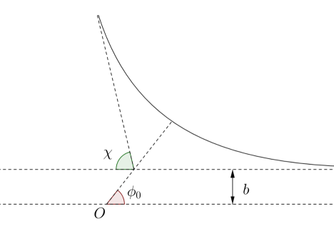
Figure 1: The two-body scattering. The solution of the two-body problem lies in a plane, which is taken to be the plane of the page. The scatterer lies in the origin. The scalar $b$ is the impact parameter and $\chi=\chi(b,V)$ is the scattering angle.

The path of the particle in the central field is symmetrical about a line from the centre to the nearest point in the orbit, hence the two asymptotes to the orbit make equal angles $\phi_{0}$ with this line (see e.g. Figure 1). The angle of scattering is seen from Fig. 1 to be

$$\chi\left(b,V\right)=\pi-2\phi_{0}\;.$$ (3.22)

We will say that the scattering problem is well defined for a given value of $V$ and $b$ if the solution of the equations

$$\frac{dy}{dt}=v\ ,\ \ \frac{dv}{dt}=-\nabla\Psi_{B}\left(y\right)$$ (3.23)

satisfies:

$$\lim_{t\rightarrow-\infty}\left|y\left(t\right)\right|=\lim_{t\rightarrow\infty}\left|y\left(t\right)\right|=\infty,\ \lim_{t\rightarrow-\infty}\left|v\left(t\right)\right|=\lim_{t\rightarrow\infty}\left|v\left(t\right)\right|=V.$$ (3.24)

The effective potential reads

$$\Psi_{eff}\left(r\right)=\Psi_{B}(r)+\frac{b^{2}V^{2}}{2r^{2}}$$ (3.25)

where $r=\left|y\right|.$ A sufficient condition for the scattering problem to be well defined for a given value of $V$ and almost all the values of $b$ is that the set of nontrivial solutions $r$ of the simultaneous equations

$$\frac{\Psi_{B}{}^{\prime}(r)}{V^{2}}=\frac{b^{2}}{r^{3}}\ ,\ \ \frac{\Psi_{B}(r)}{V^{2}}+\frac{b^{2}}{2r^{2}}=\frac{1}{2}$$ (3.26)

is nonempty only for a finite set of values $b>0.$ We will assume that this condition is satisfied for all the families of potentials considered. A standard analysis of Newton equations shows that the scattering angle is given by

$$\chi\left(b,V\right)=\pi-2\phi_{0}=\pi-2\int_{r_{\ast}}^{+\infty}\frac{b\,dr}{r^{2}\sqrt{1-2\Psi_{eff}\left(r\right)/V^{2}}}$$ (3.27)

where $r_{\ast}$ is the nearest approach of the particle to the scatterer (defined as the largest solution to the second equation in (3.26)).

Using spherical coordinates with north pole $\frac{v}{\left|v\right|}$ and azimuth angle $\varphi$ characterizing the plane of scattering, we define a mapping

$$\left(b,\varphi\right)\rightarrow\omega=\omega\left(b,\varphi;v\right)\in S^{2},$$ (3.28)

where $\omega$ is the unit vector in the direction of the velocity of the particle as $t\to+\infty$. Let $\Sigma\left(v\right)\subset S^{2}$ be the image of this mapping. Due to the symmetry of the potential $\Psi$ the set $\Sigma\left(v\right)$ is invariant under rotations around $\frac{v}{\left|v\right|}.$

We do not need to assume that the mapping (3.28) is injective in the variable $b$. In particular, a point $\omega\in\Sigma\left(v\right)$ can have different preimages. We will consider only potentials $\Psi$ for which the number of these preimages is finite. We can then define a family of inverse functions

$$\omega\rightarrow\left(b_{j}\left(\omega\right),\varphi_{j}\left(\omega\right)\right)\ \ ,\ \ j\in J\left(\omega\right)$$

where $J\left(\omega\right)$ is a set of indexes which characterizes the number of preimages of $\omega$ for each $\omega\in\Sigma\left(v\right).$ We classify the points of $\Sigma\left(v\right)$ by means of the number of preimages, i.e. we write $\bigcup_{k=1}^{\infty}A_{k}\left(v\right)=\Sigma\left(v\right)$ with

$$A_{k}\left(v\right):=\left\{\omega\in\Sigma\left(v\right):\#J\left(\omega\right)=k\right\}\ ,\ \ k=1,2,3,...$$ (3.29)

Let $\chi_{A_{k}\left(v\right)}\left(\omega\right)$ be the characteristic function of the set $A_{k}(v)$. We define the differential cross-section of the scattering problem as $\frac{1}{|v|}B$ where

$$B\left(v;\omega\right) =\sum_{k=1}^{\infty}B_{k}\left(v;\omega\right)\chi_{A_{k}\left(v\right)}\left(\omega\right)\ \ \ \ ,\ \ \ \ \omega\in\Sigma\left(v\right)\;,$$ (3.30)

$$\frac{1}{|v|}B_{k}\left(v;\omega\right) =\sum_{j\in J\left(\omega\right)}\frac{b_{j}}{|\sin\chi|}\Big{|}\left(\frac{\partial\chi\left(b_{j},V\right)}{\partial b}\right)^{-1}\Big{|}\ \ \ \ \text{for }\omega\in A_{k}\left(v\right)\;.$$ (3.31)

Since the dynamics defined by the equations (3.23) is invariant under time reversal $\left(y,v,t\right)\rightarrow\left(y,-v,-t\right)$, the following detailed balance condition holds:

$$B_{k}\left(v;\omega\right)=B_{k}\left(\left|v\right|\omega;\frac{v}{\left|v\right|}\right)\;.$$ (3.32)

With a slight abuse, we will use in what follows the same notation for cutoffed and uncutoffed ($M\to\infty$) potential.

3.1.2 Kinetic equations.

We focus first on the case of Holtsmark fields with one single charge ($L=1$, $Q_{1}=1$).

Claim 3.3

Suppose that (3.21) holds. Let us assume that $\Psi$ is as in Definition 3.1. Suppose that the following limit exists:

$$f_{\varepsilon}\left(T_{BG}t,T_{BG}x,v\right)\rightarrow f\left(t,x,v\right)\text{ as }\varepsilon\rightarrow 0\;.$$ (3.33)

Then $f$ solves the linear Boltzmann equation

$$\left(\partial_{t}f+v\partial_{x}f\right)\left(t,x,v\right)=\int_{S^{2}}B\left(v;\omega\right)\left[f\left(t,x,\left|v\right|\omega\right)-f\left(t,x,v\right)\right]d\omega$$ (3.34)

where $B$ is as in (3.30).

Justification of the Claim 3.3. We introduce a time scale $t_{\ast}$ satisfying $1\ll t_{\ast}\ll T_{BG}.$ We define the domain $D_{\varepsilon}\left(vt_{\ast}\right)\subset\mathbb{R}^{3}$ as the set swept out by the sphere of radius $M\lambda_{\varepsilon}$ initially centered at the tagged particle, moving in the direction of $v$ during the time $t_{\ast}$ (cf. (3.9)). The motion of the tagged particle is rectilinear between collisions and is affected by the interaction $\Phi_{B}$ if the domain $D_{\varepsilon}\left(vt_{\ast}\right)$ contains one or more scatterers. Notice that the volume of $D_{\varepsilon}\left(vt_{\ast}\right)$ satisfies $\left|D_{\varepsilon}\left(vt_{\ast}\right)\right|\simeq\pi VM^{2}\lambda_{\varepsilon}^{2}t_{\ast}\ll 1$ where $V=|v|$. Using the properties of the Poisson distribution it follows that the probability of finding one scatterer in $D_{\varepsilon}\left(vt_{\ast}\right)$ is approximately $\left|D_{\varepsilon}\left(vt_{\ast}\right)\right|$ and the probability of finding two or more scatterers is proportional to $\left|D_{\varepsilon}\left(vt_{\ast}\right)\right|^{2}$ which can be neglected. We introduce a system of spherical coordinates having $\frac{v}{\left|v\right|}$ as north pole and we denote by $\varphi$ the azimuth angle (as in Section 3.1.1). Assuming that there is one scatterer in the domain $D_{\varepsilon}\left(vt_{\ast}\right)$, the conditional probability that the scatterer has azimuth angle in the interval $\left[\varphi,\varphi+d\varphi\right]$ and the impact parameter of the collision is in the interval $\left[\bar{b},\bar{b}+d\bar{b}\right]$ can be approximated by $\frac{Vt_{*}\bar{b}d\bar{b}d\varphi}{\left|D_{\varepsilon}\left(vt_{\ast}\right)\right|}$. We obtain deflections in the velocity $v$ of order one if $\bar{b}$ is of order $\lambda_{\varepsilon},$ therefore it is natural to introduce the change of variables $\bar{b}=\lambda_{\varepsilon}b.$ We conclude that the probability of a collision in a time interval of length $t_{\ast}$ with rescaled impact parameter $b$ and azimuth angle $\varphi$ is:

$$\left(\lambda_{\varepsilon}\right)^{2}Vt_{\ast}bdbd\varphi.$$ (3.35)

In order to derive the evolution equation for the function $f\left(t,x,v\right)$ it is convenient to compute the limit behaviour of (cf. (3.7))

$$\psi_{\varepsilon}\left(t,x,v\right):=\mathbb{E}\left[\psi_{0,\varepsilon}\left(T^{t}\left(x,v;\varepsilon;\cdot\right)\right)\right]$$ (3.36)

where $\psi_{0,\varepsilon}=\psi_{0,\varepsilon}\left(x,v\right)$ is a smooth test function. We have the following duality formula

$$\int\int f_{\varepsilon}\left(t,x,v\right)\psi_{0,\varepsilon}\left(x,v\right)dxdv=\int\int f_{0}(x,v)\psi_{\varepsilon}\left(t,x,v\right)dxdv\ \ ,\ \ t>0$$ (3.37)

which follows using (3.7), the change of variables $T^{-t_{0}}\left(x,v;\varepsilon;\cdot\right)=\left(y,w\right),$ and (3.36). We compute the differential equation satisfied by the function $\psi\left(t,x,v\right)=\lim_{\varepsilon\rightarrow 0}\psi_{\varepsilon}\left(T_{BG}t,T_{BG}x,{v}\right)$ with $\psi_{0}\left(x,v\right)=\lim_{\varepsilon\rightarrow 0}\psi_{0,\varepsilon}\left(T_{BG}x,v\right).$ Supposing that $h>0$ is small but such that $hT_{BG}\gg 1$ and using the semigroup property of $T^{t}$ we obtain

$$\psi_{\varepsilon}\left(T_{BG}(t+h),T_{BG}x,v\right) =\mathbb{E}\left[\psi_{0,\varepsilon}\left(T^{T_{BG}(t+h)}\left(T_{BG}x,v;\varepsilon;\cdot\right)\right)\right]$$

$$=\mathbb{E}\left[\psi_{0,\varepsilon}\left(T^{T_{BG}h}T^{T_{BG}t}\left(T_{BG}x,v;\varepsilon;\cdot\right)\right)\right].$$ (3.38)

We assume now that the deflection of the particle during $\left[T_{BG}t,T_{BG}(t+h)\right]$ is independent from its previous evolution in $\left[0,T_{BG}t\right]$ (in particular, recollisions of the particle with the scatterers happen with small probability). To prove this independence would be a crucial step of any rigorous proof of the Claim 3.3 (notice that this implies also the Markovianity of the limit process). Then

$$\psi_{\varepsilon}\left(T_{BG}(t+h),T_{BG}x,v\right)\simeq\mathbb{E}\left[\psi_{\varepsilon}\left(T_{BG}t,T^{T_{BG}h}\left(T_{BG}x,v;\varepsilon;\cdot\right)\right)\right]$$ (3.39)

for small $\varepsilon>0$. If the position of the particle is $\left(T_{BG}x,v\right)$ at the time $T_{BG}t,$ its new position at the time $T_{BG}(t+h)$ is $T_{BG}x+vT_{BG}h.$ Recalling the expression (3.35) for the probability of a collision with given impact parameter and azimuth angle, we deduce

$$\psi_{\varepsilon}\left(T_{BG}(t+h),T_{BG}x,v\right)$$

$$\simeq\psi_{\varepsilon}\left(T_{BG}t,T_{BG}x+vT_{BG}h,v\right)\left[1-\left(\lambda_{\varepsilon}\right)^{2}VhT_{BG}\int_{0}^{2\pi}d\varphi\int_{0}^{M}bdb\right]+$$

$$+\left(\lambda_{\varepsilon}\right)^{2}VT_{BG}h\int_{0}^{2\pi}d\varphi\int_{0}^{M}bdb\,\psi_{\varepsilon}\left(T_{BG}t,T_{BG}x,\left|v\right|\omega\left(b,\varphi;v\right)\right)$$

where $\omega\left(b,\varphi;v\right)$ is as in (3.28). Here we neglected the probability of having more than one collision in the time interval $[T_{BG}t,T_{BG}(t+h)]$, since $h$ is sufficiently small. Using $T_{BG}\lambda_{\varepsilon}^{2}=1$ and a Taylor expansion in $h$, we obtain, in the limit $h\rightarrow 0$,

$$\frac{\partial\psi\left(t,x,v\right)}{\partial\tau}=v\frac{\partial\psi\left(t,x,v\right)}{\partial x}+V\int_{0}^{2\pi}d\varphi\int_{0}^{M}bdb\left[\psi\left(t,x,\left|v\right|\omega\left(b,\varphi;v\right)\right)-\psi\left(t,x,v\right)\right].$$ (3.40)

Finally, we pass to the limit in (3.37). We set $f(t,x,v)=\lim_{\varepsilon\rightarrow 0}f_{\varepsilon}\left(T_{BG}t,T_{BG}x,v\right)$, $f_{0}(x,v)=f\left(0,x,v\right)$ and $\bar{\psi}\left(t,x,v\right)=\psi\left(t_{0}-t,x,v\right)$ for $t_{0}>0$. We get

$$\int\int f\left(t_{0},x,v\right)\bar{\psi}\left(t_{0},x,v\right)dxdv=\int\int f_{0}(x,v)\bar{\psi}_{0}\left(x,v\right)dxdv\ \ \ ,\ t_{0}>0$$

which implies

$$\partial_{t}\left(\int\int f\left(t,x,v\right)\bar{\psi}\left(t,x,v\right)dxdv\right)=0\;.$$ (3.41)

Note that, by (3.40), for $0<t<t_{0}$ we have

$$\frac{\partial\bar{\psi}\left(t,x,v\right)}{\partial t} =-v\frac{\partial\bar{\psi}\left(t,x,v\right)}{\partial x}-V\int_{0}^{2\pi}d\varphi\int_{0}^{M}bdb\left[\bar{\psi}\left(t,x,\left|v\right|\omega\left(b,\varphi;v\right)\right)-\bar{\psi}\left(t,x,v\right)\right]\;,$$

$$\bar{\psi}\left(t_{0},x,v\right) =\psi_{0}\left(x,v\right).$$ (3.42)

Using (3.41) and (3.42) and integrating by parts in the term containing $\partial_{x}$ we obtain

$$0 =\int\int\bar{\psi}\left(t,x,v\right)\partial_{t}f\left(t,x,v\right)dxdv+\int\int\bar{\psi}\left(t,x,v\right)v\partial_{x}f\left(t,x,v\right)dxdv-$$

$$-\int\int dxdv\int_{0}^{2\pi}d\varphi\left|v\right|\int_{0}^{M}bdb\left[\bar{\psi}\left(t,x,\left|v\right|\omega\left(b,\varphi;v\right)\right)-\bar{\psi}\left(t,x,v\right)\right]f\left(t,x,v\right).$$ (3.43)

Performing the change of variables in (3.28) (cf. (3.31)) and taking then the limit $M\rightarrow\infty$ we can write the last integral term in (3.43) as

$$-\int\int dxdv\,\bar{\psi}\left(t,x,v\right)\sum_{k=1}^{\infty}\int_{A_{k}\left(v\right)}\left[B_{k}\left(\left|v\right|\omega;\frac{v}{\left|v\right|}\right)f\left(t,x,\left|v\right|\omega\right)-B_{k}\left(v;\omega\right)f\left(t,x,v\right)\right]d\omega\;.\\$$ (3.44)

From (3.30), (3.32) and the arbitrariness of $\bar{\psi}$, we get (3.34).   

Remark 3.4

The above way of obtaining the Boltzmann equation is reminiscent of the cutoff procedure used in [13] to derive the Boltzmann equation rigorously for potentials of the form $|x|^{-s}$ for $s>2$ in two space dimensions.

Remark 3.5

The condition (3.21) enters in the argument because we assume that the trajectories of the particles between collisions are rectilinear. This is due to the fact that the time $T_{L}$ required to produce deflections between collisions is much larger than the scale $T_{BG}$.

Remark 3.6

If the Holtsmark field in which the particle evolves has different types of charges we must replace (3.34) by the equation

$$\left(\partial_{t}f+v\partial_{x}f\right)\left(t,x,v\right)=\sum_{j=1}^{L}\mu\left(Q_{j}\right)\int_{S^{2}}B\left(v;\omega;Q_{j}\right)\left[f\left(t,x,\left|v\right|\omega\right)-f\left(t,x,v\right)\right]d\omega$$

where $B\left(v;\omega;Q_{j}\right)$ is the scattering kernel obtained computing the deflections for each type of charge. Notice that the form of $\Psi_{eff}$ in (3.25) yields the following functional dependence for the differential cross-section $\Sigma=B/|v|$:

$$\Sigma\left(v;\omega;Q_{j}\right)=\Sigma\left(\frac{v}{\sqrt{\left|Q_{j}\right|}};\omega;\operatorname*{sgn}\left(Q_{j}\right)\right)$$

i.e. we can reduce the computation of the scattering kernel to just two values of the charge $\pm 1$ and arbitrary particle velocities. Notice that there is no reason to expect $B$ to take the same value for positive and negative charges and a given value of the velocity, although it turns out that this happens in the particular case of Coulomb potentials.

3.2 Kinetic equations describing the evolution of the distribution function $f:$ the Landau case.

In this section we consider the evolution of the function $f_{\varepsilon}$ defined in (3.7) as $\varepsilon\rightarrow 0,$ assuming (3.17) and (3.19). The latter condition is not sufficient to obtain a Landau equation, since we need also to have independent deflections on time scales of order $T_{L}.$ Under the conditions yielding the Landau equation the deflections in times of order $T_{L}$ are gaussian variables and the independence condition reads (cf. (3.11))

$$\mathbb{E}\left(D(0)\,D(\tilde{T}_{L})\right)\ll\sqrt{\mathbb{E}\left(D(0)^{2}\right)\mathbb{E}\left(D(\tilde{T}_{L})^{2}\right)}\ \ \text{as\ \ }\varepsilon\rightarrow 0$$ (3.45)

where $\tilde{T}_{L}$ is some time scale much smaller than $T_{L}$, and we denoted $D\left(0\right)$ and $D(\tilde{T}_{L})$ the deflections experienced during the time intervals $\left[0,\tilde{T}_{L}\right],\ \left[\tilde{T}_{L},2\tilde{T}_{L}\right]$ respectively. Furthermore, in order to have a well defined probability distribution for the deflections we need the convergence as $\varepsilon\to 0$ of the characteristic function $m_{T}^{(\varepsilon)}\left(\theta\right)$ in (3.14). More precisely, restricting for simplicity to the case of one single charge and assuming $|v|=1$, we have

$$\frac{1}{2}\int_{\mathbb{R}^{3}}\left(\theta\cdot\int_{0}^{\zeta T_{L}}dt\,\nabla_{x}\Phi_{L}\left(v\zeta T_{L}-y,\varepsilon\right)\right)^{2}dy\rightarrow\kappa\,\zeta\left|\theta_{\bot}\right|^{2}\ \text{as\ }\varepsilon\rightarrow 0$$ (3.46)

for every $\zeta>0$ and for some constant $\kappa>0,$ where $\theta_{\bot}=\theta-\frac{\theta\cdot v}{\left|v\right|}\frac{v}{\left|v\right|}.$ In particular,

$$m_{\zeta T_{L}}^{(\varepsilon)}\left(\theta\right)\rightarrow\exp\left(-\kappa\zeta\left|\theta_{\bot}\right|^{2}\right)\ \ \text{as\ }\varepsilon\rightarrow 0.$$ (3.47)

We will not try to formulate the most general set of conditions under which (3.46) takes place. However, we can expect this formula to be a consequence of the smallness of the deflections, the independence condition (3.45) and the x limit theorem. We will show in Section 4 examples of families of potentials for which the left-hand side of (3.46) converges to a different quadratic form. For those families of potentials (3.45) also fails. Moreover, the following simple argument sheds some light on the relation between (3.45) and (3.46). Suppose that the deflections of the tagged particle in the time intervals $\left[0,\zeta_{1}T_{L}\right]$ and $\left[\zeta_{1}T_{L},\left(\zeta_{1}+\zeta_{2}\right)T_{L}\right]$, denoted by $D_{1}$ and $D_{2}$, are independent (at least asymptotically as $\varepsilon\rightarrow 0$). Then the characteristic function $m_{(\zeta_{1}+\zeta_{2})T_{L}}^{(\varepsilon)}\left(\theta\right)$ of the total deflection $D=D_{1}+D_{2}$ is close to a product $m_{\zeta_{1}T_{L}}^{(\varepsilon)}\left(\theta\right)m_{\zeta_{2}T_{L}}^{(\varepsilon)}\left(\theta\right)$. This is possible only if the function on the right-hand side of (3.46) is linear in $\zeta$ (cf. (3.47)).

In the following we assume both (3.45) and (3.46) and we derive a linear Landau equation.

Claim 3.7

Assume that (3.19) holds and suppose that (3.45), (3.46) are also satisfied. Suppose that the following limit exists:

$$f_{\varepsilon}\left(T_{L}t,T_{L}x,v\right)\rightarrow f\left(t,x,v\right)\text{ as }\varepsilon\rightarrow 0.$$ (3.48)

Then

$$\left(\partial_{t}f+v\partial_{x}f\right)\left(t,x,v\right)=\kappa\Delta_{v_{\perp}}f\left(t,x,v\right)$$ (3.49)

where $\Delta_{v_{\perp}}$ is the Laplace Beltrami operator on $S^{2}$ (sphere of radius $|v|=1$) and the diffusion coefficient $\kappa>0$ is defined by (3.46).

Remark 3.8

Using Cartesian coordinates, the diffusion term in (3.49) reads as

$$\sum_{i,j=1}^{3}\frac{\partial}{\partial v_{i}}A_{i,j}(v)\frac{\partial}{\partial v_{j}}f\left(t,x,v\right)$$ (3.50)

where the diffusion matrix $A_{i,j}(v)$ is given by

$$A_{i,j}(v)=\kappa\left(\delta_{ij}-\frac{v_{i}v_{j}}{|v|^{2}}\right)\;.$$ (3.51)

We refer to [23] and [28] for further details.

Justification of the Claim 3.7. Using (3.47) and the Fourier inversion formula, we can compute the probability density for the transition from $\left(T_{L}x,v\right)$ to $\left(T_{L}y,v+D\right)$ in a time interval of length $T_{L}h$ with $D\in\mathbb{R}^{3}:$

$$p\left(T_{L}y,v+D;T_{L}x,v;T_{L}h\right) =\frac{\delta\left(T_{L}y-T_{L}x-vT_{L}h\right)T_{L}^{3}}{\left(2\pi\right)^{3}}\int_{\mathbb{R}^{3}}\exp\left(-\kappa h\left|\theta_{\bot}\right|^{2}\right)\exp\left(iD\cdot\theta\right)d\theta$$

$$=\frac{\delta\left(T_{L}y-T_{L}x-vT_{L}h\right)\delta\left(D_{\parallel}\right)T_{L}^{3}}{4\kappa\pi h}\exp\left(-\frac{\left|D_{\perp}\right|^{2}}{\kappa h}\right)\;.$$

Here we write $\theta=\left(\theta_{\parallel},\theta_{\bot}\right)$ with

$$\theta_{\parallel}=\theta\cdot\frac{v}{\left|v\right|},\ \ \ \ \theta_{\bot}=\theta-\left(\theta\cdot\frac{v}{\left|v\right|}\right)\frac{v}{\left|v\right|}$$ (3.52)

and use a similar decomposition for $D=\left(D_{\parallel},D_{\perp}\right)$ and other vectors appearing later. That is, the probability density yielding the transition from $\left(T_{L}x,v\right)$ to $\left(T_{L}y,w\right)$ is

$$p\left(T_{L}y,w;T_{L}x,v;T_{L}h\right)=\frac{\delta\left(x-y-vh\right)\delta\left(v_{\parallel}-w_{\parallel}\right)}{4\kappa\pi h}\exp\left(-\frac{\left|v_{\perp}-w_{\perp}\right|^{2}}{\kappa h}\right)\equiv G(y,w;x,v;h)\;.$$ (3.53)

Using the independence assumption, we obtain the following approximation for $h$ small

$$f_{\varepsilon}\left(T_{L}(t+h),T_{L}x,v\right)\simeq\int_{\mathbb{R}^{3}}dy\int_{\mathbb{R}^{3}}dwf_{\varepsilon}\left(T_{L}t,T_{L}y,w;\varepsilon\right)p\left(T_{L}y,w;T_{L}x,v;T_{L}h\right)$$

whence, using (3.48),

$$f\left(t+h,x,v\right)=\int_{\mathbb{R}^{3}}dy\int_{\mathbb{R}^{3}}dwf\left(t,y,w\right)G\left(y,w;x,v;h\right)$$

and by (3.53)

$$f\left(t+h,x,v\right) =\frac{1}{4\kappa\pi h}\int_{\mathbb{R}^{2}}dw_{\bot}f\left(t,x-vh,v_{\parallel},w_{\bot}\right)\exp\left(-\frac{\left|v_{\perp}-w_{\perp}\right|^{2}}{\kappa h}\right)\;.$$

Approximating $f\left(t,y,w\right)$ by means of its Taylor expansion up to second order in $w_{\bot}=v_{\bot}$ and to first order in ${y}={x}$ as well as $f\left(t+h,x,v\right)$ by its first order Taylor expansion in $h=0$, we obtain (3.49).   

3.3 The case of deflections with correlations of order one.

If (3.17) and $T_{L}\ll T_{BG}$ hold but the condition (3.45) fails, then the dynamics of the distribution function $f_{\varepsilon}$ cannot be approximated by means of a Landau equation. We shall not consider this case in detail in this paper. However it is interesting to formulate the type of mathematical problem describing the dynamics of the tagged particle. We discuss such formulation in the present section.

We denote the deflection experienced by the tagged particle at the point $x,$ with initial velocity $v$ during a small (eventually infinitesimal) time $h$ as $D\left(x,v;h\right).$ We use here macroscopic variables for space and time. As $\varepsilon\to 0$, the characteristic function of $D$ approaches the exponential of a quadratic function and the deflections become gaussian variables with zero average. For these variables, the form of the correlation might be strongly dependent on the family of potentials considered, but some general features might be expected.

First of all, due to the invariance under translation of the Holtsmark field, the correlation functions will take the form

$$\mathbb{E}\left[D\left(x_{1},v_{1};h\right)\otimes D\left(x_{2},v_{2};h\right)\right]=K\left(x_{1}-x_{2},v_{1},v_{2};h\right)\neq 0.$$ (3.54)

Furthermore, we will obtain (cf. examples in Section 4)

$$\int_{0}^{1}K\left(y(s),v_{1},v_{2};h\right)ds<\infty$$ (3.55)

for any curve $y(s)$ of class $C^{1}$. This integrability condition might be expected if (3.45) fails, because otherwise one could have large deflections at small distances and $T_{L}$ would not coincide with the scale of the mean free path (cf. (3.17)).

Finally, the equation yielding the evolution of the tagged particle can be written as

$$x\left(\tau+d\tau\right)-x\left(\tau\right)=v(\tau)d\tau\ \ ,\ \ v\left(\tau+d\tau\right)-v\left(\tau\right)=D\left(x\left(\tau\right),v\left(\tau\right);d\tau\right)\;,$$ (3.56)

where the order of magnitude of $D$ is not necessarily $d\tau$, but it might be of order $(d\tau)^{\alpha^{\prime}}$ for some $0<\alpha^{\prime}<1$ (see e.g. Section 4.2.3, $\frac{1}{2}<s<1$).

A typical example which can be derived for a family of power law potentials is the following (cf. Theorem 4.3-(ii)):

$$K\left(y,v_{1},v_{2};d\tau\right)=\frac{1}{\left|y\right|^{\alpha}}\Lambda\left(\frac{y}{\left|y\right|},v_{1},v_{2}\right)\left(d\tau\right)^{2}\ \ ,\ y\neq 0\ ,\ \ \ 0<\alpha<1\ \ ,\ \$$ (3.57)

$$K\left(0,v_{1},v_{2};d\tau\right)=\Lambda\left(v_{1},v_{2}\right)\left(d\tau\right)^{2-\alpha}\;,$$ (3.58)

where $\Lambda$ is a matrix valued function. Note that, likely, due to the integrability of the factor $\frac{1}{\left|y\right|^{\alpha}}$ in (3.57), the condition (3.58) does not play a relevant role.

It would be interesting to clarify if (3.54)-(3.58) forms a well defined mathematical problem which can be solved for a suitable choice of initial values $x\left(0\right)=x_{0},\ v\left(0\right)=v_{0}.$ Note that this is not a standard stochastic differential equation, but rather a stochastic differential equation with correlated noise. The dynamics (3.56) has some analogies with fractional Brownian motion [25].

4 Examples of kinetic equations derived for different families of potentials.

We now apply the formalism of Section 3 to different families of potentials. First we check if the families of potentials considered have an associated collision length, then we examine the behaviour of the functions $\sigma\left(T;\varepsilon\right)$ in (3.15). We compute the time scales $T_{BG},\ T_{L}$ defined in (3.3), (3.16) and check if (3.17) and some of the conditions (3.18)-(3.21) and (3.45)-(3.46) hold. Finally, we write the corresponding kinetic equations.

4.1 Kinetic time scales for potentials with the form $\Phi\left(x,\varepsilon\right)=\Psi\left(\frac{\left|x\right|}{\varepsilon}\right).$

We first consider the family of potentials

$$\left\{\Phi\left(x,\varepsilon\right);\ \varepsilon>0\right\}=\left\{\Psi\left(\frac{\left|x\right|}{\varepsilon}\right);\ \varepsilon>0\right\}$$ (4.1)

where $\Phi(\cdot,\varepsilon)\in{\cal C}_{s}$, $s>1/2$. We have $\Psi\in C^{2}\left(\mathbb{R}^{3}\setminus\left\{0\right\}\right)$ and

$$\Psi\left(y\right)\sim\frac{A}{\left|y\right|^{s}}\ \ \text{as\ \ }\left|y\right|\rightarrow\infty\ \ ,\ \ \ \nabla\Psi\left(y\right)\sim-\frac{sAy}{\left|y\right|^{s+2}}\ \ \text{as\ \ }\left|y\right|\rightarrow\infty$$ (4.2)

for some real number $A\neq 0$ (cf. (2.7)). By Definition 3.1, the collision length is $\lambda_{\varepsilon}=\varepsilon$ and

$$T_{BG}=\frac{1}{\varepsilon^{2}}\;.$$ (4.3)

It is possible to state some general result for these potentials which depends only on the asymptotics of $\Psi\left(y\right)$ as a power law as $\left|y\right|\rightarrow\infty.$

Theorem 4.1

Consider the family of potentials (4.1) with $\Phi(\cdot,\varepsilon)\in{\cal C}_{s}$, $s>1/2$. Suppose that the corresponding Holtsmark field defined in Section 2 is spatially homogeneous. Then

$$\lim\sup_{\varepsilon\rightarrow 0}\sigma\left(T_{BG};\varepsilon\right)\leq\delta\left(M\right)\ \ \text{with\ }\lim_{M\rightarrow\infty}\delta\left(M\right)=0\quad\text{if}\quad s>1$$ (4.4)

where $\sigma\left(T;\varepsilon\right)$ is defined in (3.15). If we define $T_{L}$ by means of (3.16) we have

$$T_{L}\sim\frac{1}{4\pi A^{2}\varepsilon^{2}\log\left(\frac{1}{\varepsilon}\right)}\ \ \text{as\ \ }\varepsilon\rightarrow 0\quad\text{if }\quad s=1$$ (4.5)

and

$$T_{L}\sim\left(\frac{1}{W_{s}A^{2}\varepsilon^{2s}}\right)^{\frac{1}{3-2s}}\ \ \text{as\ \ }\varepsilon\rightarrow 0\quad\text{if}\quad\frac{1}{2}<s<1$$ (4.6)

with

$$W_{s}=\sup_{|\theta|=1}\int_{\mathbb{R}^{3}}d\xi\left[s^{2}\left(\theta_{\bot}\cdot\xi_{\bot}\right)^{2}\left(\int_{0}^{1}\frac{d\tau}{\left|v\tau-\xi\right|^{s+2}}\right)^{2}+\theta_{\parallel}^{2}\,\left(\frac{1}{\left|\xi\right|^{s}}-\frac{1}{\left|\xi-v\right|^{s}}\right)^{2}\right]$$ (4.7)

(cf. (3.52)), whence

$$T_{L}\ll T_{BG}\ \ \text{as }\ \ \varepsilon\rightarrow 0\quad\text{if }\quad s\leq 1.$$

Remark 4.2

We recall that the assumption of spatial homogeneity for the Holtsmark field means that we need to consider neutral distributions of charges or distributions with a background charge if $s\leq 1.$

4.1.1 Proof of Theorem 4.1: general strategy.

We use the splitting (3.8) which in the case of the family (4.1) becomes $\Phi\left(x,\varepsilon\right)=\Phi_{B}\left(x,\varepsilon\right)+\Phi_{L}\left(x,\varepsilon\right)$ with

$$\Phi_{B}\left(x,\varepsilon\right)=\Psi_{B,M}\left(\frac{x}{\varepsilon}\right)\ \ ,\ \ \Phi_{L}\left(x,\varepsilon\right)=\Psi_{L,M}\left(\frac{x}{\varepsilon}\right)\;,\$$ (4.8)

$$\Psi_{B,M}\left(y\right)=\Psi\left(y\right)\eta\left(\frac{y}{M}\right)\ \ ,\ \ \Psi_{L,M}\left(y\right)=\Psi\left(y\right)\left[1-\eta\left(\frac{y}{M}\right)\right].$$ (4.9)

We study the asymptotic properties of the function

$$\sigma\left(T;\varepsilon\right)=\sup_{\left|\theta\right|=1}\int_{\mathbb{R}^{3}}dy\left(\theta\cdot\int_{0}^{T}\nabla_{x}\Phi_{L}\left(vt-y,\varepsilon\right)dt\right)^{2}$$ (4.10)

separately for the three different ranges $s>1,\ s=1$ and $\frac{1}{2}<s<1$ and assuming $|v|=1$.

4.1.2 Proof of Theorem 4.1: the case $s>1$.

Our goal is to prove (4.4). To this end we first notice that (3.15) and (4.3) imply

$$\sigma\left(T_{BG};\varepsilon\right)=\frac{1}{\varepsilon^{8}}\sup_{\left|\theta\right|=1}\int_{\mathbb{R}^{3}}d\xi\left(\frac{\theta}{\varepsilon^{2}}\cdot\int_{0}^{1}\nabla\Psi_{L,M}\left(\frac{v\tau-\xi}{\varepsilon^{3}}\right)d\tau\right)^{2}\;.$$

We use that $\left|\nabla\Psi_{L,M}\right|\leq\frac{C\chi_{\left[M,\infty\right)}\left(\left|y\right|\right)}{\left|y\right|^{s+1}}$ for some $C>0$, where we denote as $\chi_{A}$ the characteristic function of the set $A.$ Then

$$\sigma\left(T_{BG};\varepsilon\right)\leq\frac{C}{\varepsilon^{8}}\int_{\mathbb{R}^{3}}d\xi\left(\frac{\varepsilon^{3\left(s+1\right)}}{\varepsilon^{2}}\int_{0}^{1}\frac{\chi_{\left[M,\infty\right)}\left(\frac{\left|v\tau-\xi\right|}{\varepsilon^{3}}\right)}{\left|v\tau-\xi\right|^{s+1}}d\tau\right)^{2}.$$ (4.11)

We split the integral as $\int_{\mathbb{R}^{3}}\left[\cdot\cdot\cdot\right]d\xi=\int_{\left\{\left|\xi\right|\geq 2\right\}}\left[\cdot\cdot\cdot\right]d\xi+\int_{\left\{\left|\xi\right|<2\right\}}\left[\cdot\cdot\cdot\right]d\xi$ and notice that the first term is

$$\int_{\left\{\left|\xi\right|\geq 2\right\}}\left[\cdot\cdot\cdot\right]d\xi\leq C\varepsilon^{6\left(s-1\right)}\int_{\left\{\left|\xi\right|\geq 2\right\}}\frac{d\xi}{\left|\xi\right|^{2\left(s+1\right)}}\leq C\varepsilon^{6\left(s-1\right)}.$$ (4.12)

We split again the second domain as

$$\left\{\left|\xi_{\bot}\right|\geq\frac{M\varepsilon^{3}}{2},\ \left|\xi\right|<2\right\}\cup\left\{\left|\xi_{\bot}\right|<\frac{M\varepsilon^{3}}{2},\ \left|\xi\right|<2\right\}$$

where $\eta=\left(\eta_{\parallel},\eta_{\bot}\right)$ (as in (3.52)). Note that $\left|v\tau-\xi\right|^{s+1}=\left(\left(\tau-\xi_{\parallel}\right)^{2}+\left(\xi_{\bot}\right)^{2}\right)^{\frac{s+1}{2}}$. If $\left|\xi_{\bot}\right|\geq\frac{M\varepsilon^{3}}{2}$ we use

$$\int_{0}^{1}\frac{\chi_{\left[M,\infty\right)}\left(\frac{\left|v\tau-\xi\right|}{\varepsilon^{3}}\right)}{\left|v\tau-\xi\right|^{s+1}}d\tau\leq\int_{-\infty}^{\infty}\frac{d\tau}{\left(\tau^{2}+\left(\xi_{\bot}\right)^{2}\right)^{\frac{s+1}{2}}}\leq\frac{C}{\left|\xi_{\bot}\right|^{s}}.$$ (4.13)

Otherwise if $\left|\xi_{\bot}\right|<\frac{M\varepsilon^{3}}{2},$ since the integrand is different from zero only if $\frac{\left|v\tau-\xi\right|}{\varepsilon^{3}}\geq M,$ we must have $\left|\tau-\xi_{\parallel}\right|\geq\frac{M\varepsilon^{3}}{2}$ to have a nontrivial contribution, hence

$$\int_{0}^{1}\frac{\chi_{\left[M,\infty\right)}\left(\frac{\left|v\tau-\xi\right|}{\varepsilon^{3}}\right)}{\left|v\tau-\xi\right|^{s+1}}d\tau \leq\int_{\left[0,1\right]\cap\left\{\left|\tau-\xi_{\parallel}\right|\geq\frac{M\varepsilon^{3}}{2}\right\}}\frac{d\tau}{\left(\left(\tau-\xi_{\parallel}\right)^{2}+\left(\xi_{\bot}\right)^{2}\right)^{\frac{s+1}{2}}}$$

$$\leq\frac{1}{\left|\xi_{\bot}\right|^{s}}\int_{\left\{\left|\tau\right|\geq\frac{M\varepsilon^{3}}{2\left|\xi_{\bot}\right|}\right\}}\frac{d\tau}{\left(\tau^{2}+1\right)^{\frac{s+1}{2}}}\leq\frac{C}{M^{s}\varepsilon^{3s}}.$$ (4.14)

Combining (4.13) and (4.14) we get

$$\int_{0}^{1}\frac{\chi_{\left[M,\infty\right)}\left(\frac{\left|v\tau-\xi\right|}{\varepsilon^{3}}\right)}{\left|v\tau-\xi\right|^{s+1}}d\tau\leq\frac{C}{\left(\max\left\{\left|\xi_{\bot}\right|,M\varepsilon^{3}\right\}\right)^{s}}.$$

Plugging this estimate into the term $\int_{\left\{\left|\xi\right|<2\right\}}\left[\cdot\cdot\cdot\right]d\xi$ (cf. (4.11)) we arrive at

$$\frac{1}{\varepsilon^{8}}\int_{\left\{\left|\xi\right|<2\right\}}d\xi\left(\frac{\varepsilon^{3\left(s+1\right)}}{\varepsilon^{2}}\int_{0}^{1}\frac{\chi_{\left[M,\infty\right)}\left(\frac{\left|v\tau-\xi\right|}{\varepsilon^{3}}\right)}{\left|v\tau-\xi\right|^{s+1}}d\tau\right)^{2}$$

$$\leq\frac{C}{\varepsilon^{8}}\int_{-2}^{2}d\xi_{\parallel}\int_{\left\{\left|\xi_{\bot}\right|\leq M\varepsilon^{3}\right\}}d\xi_{\bot}\left(\frac{\varepsilon^{3\left(s+1\right)}}{\varepsilon^{2}}\frac{1}{\left(M\varepsilon^{3}\right)^{s}}\right)^{2}+$$

$$+\frac{C}{\varepsilon^{8}}\int_{-2}^{2}d\xi_{\parallel}\int_{\left\{\left|\xi_{\bot}\right|>M\varepsilon^{3}\right\}}d\xi_{\bot}\left(\frac{\varepsilon^{3\left(s+1\right)}}{\varepsilon^{2}}\frac{1}{\left|\xi_{\bot}\right|^{s}}\right)^{2}\leq\frac{C}{M^{2\left(s-1\right)}}\;.$$

Using this and (4.12) we obtain

$$\sigma\left(T_{BG};\varepsilon\right)\leq C\varepsilon^{6\left(s-1\right)}+\frac{C}{M^{2\left(s-1\right)}}.$$

Taking first the limit $\varepsilon\rightarrow 0$ (using $s>1$) and then $M\rightarrow\infty$ we obtain (4.4). This gives the result of Theorem 4.1 for $s>1.$

4.1.3 Proof of Theorem 4.1: the case $s=1$.

Our goal is to prove the existence of $T_{L}\ll T_{BG}$ such that $\sigma\left(T_{L};\varepsilon\right)\sim 1$ as $\varepsilon\rightarrow 0$, using (4.2) with $s=1$. We assume that $A=1,$ since $A$ can be simply absorbed as a rescaling factor.

Changing variables $y=T\xi,\ t=T\tau$ in (3.15) we can write:

$$\sigma\left(T;\varepsilon\right)=\frac{T^{3}}{\varepsilon^{2}}\sup_{\left|\theta\right|=1}\int_{\mathbb{R}^{3}}d\xi\left(T\theta\cdot\int_{0}^{1}\nabla\Psi_{L,M}\left(\frac{T(v\tau-\xi)}{\varepsilon}\right)d\tau\right)^{2}\;.$$

Let $Z=1-\eta$ (cf. (4.9)). Using (4.2) we obtain

$$\sigma\left(T;\varepsilon\right)=T\varepsilon^{2}\sup_{\left|\theta_{\bot}\right|=1}\int_{\mathbb{R}^{3}}d\xi\left(\left(\theta_{\bot}\cdot\xi_{\bot}\right)\int_{0}^{1}\frac{Z\left(\frac{T\left|v\tau-\xi\right|}{M\varepsilon}\right)}{\left|v\tau-\xi\right|^{3}}d\tau\right)^{2}\left[1+\zeta\left(M;\varepsilon\right)\right]$$ (4.15)

where $\lim\sup_{\varepsilon\rightarrow 0}|\zeta\left(M;\varepsilon\right)|\leq\zeta\left(M\right)$ and $\zeta\left(M\right)\rightarrow 0$ as $M\rightarrow\infty.$ In $\zeta\left(M;\varepsilon\right)$ we collect: (i) the errors coming from the computation of the gradient via (4.9) with the approximation (2.7) (with $s=1$ and $A=1$), which can be estimated as in the previous section; (ii) the contribution of the longitudinal component $\theta_{\parallel}$. Note that the latter yields a term of order

$$T\varepsilon^{2}\int_{\mathbb{R}^{3}}d\xi\left(\frac{Z\left(\frac{T\left|\xi\right|}{M\varepsilon}\right)}{\left|\xi\right|}-\frac{Z\left(\frac{T\left|\xi-v\right|}{M\varepsilon}\right)}{\left|\xi-v\right|}\right)^{2}\;,$$ (4.16)

which can be estimated by $CT\varepsilon^{2}.$ Since the integral in (4.15) will produce an additional contribution of the order $\log\big{(}\frac{1}{\varepsilon}\big{)}$, (4.16) can be absorbed into $\zeta\left(M;\varepsilon\right)$.

We decompose the integral $\int_{\mathbb{R}^{3}}\left[\cdot\cdot\cdot\right]d\xi$ in (4.15) as $\int_{\left\{\left|\xi\right|\geq 2\right\}}\left[\cdot\cdot\cdot\right]d\xi+\int_{\left\{\left|\xi\right|<2\right\}}\left[\cdot\cdot\cdot\right]d\xi$ and notice that the first one is bounded, so that

$$\sigma\left(T;\varepsilon\right)=T\varepsilon^{2}\sup_{\left|\theta_{\bot}\right|=1}\int_{\left\{\left|\xi\right|<2\right\}}d\xi\left(\left(\theta_{\bot}\cdot\xi_{\bot}\right)\int_{0}^{1}\frac{Z\left(\frac{T\left|v\tau-\xi\right|}{M\varepsilon}\right)}{\left|v\tau-\xi\right|^{3}}d\tau\right)^{2}\left[1+\zeta\left(M;\varepsilon\right)\right]+O(T\varepsilon^{2})\;.$$

Arguing similarly we obtain that the main contribution to the integral is due to a cylinder with principal axis $(\xi_{\parallel}\in[0,1],\xi_{\perp}=0)$ and radius much smaller than $1$. In particular

$$\sigma\left(T;\varepsilon\right)\sim T\varepsilon^{2}\int_{0}^{1}d\xi_{\parallel}\int_{\left\{\left|\xi_{\bot}\right|\leq 1\right\}}d\xi_{\bot}\left(\theta_{\bot}\cdot\xi_{\bot}\right)^{2}\left(\int_{0}^{1}\frac{Z\left(\frac{T\left|v\tau-\xi\right|}{M\varepsilon}\right)}{\left|v\tau-\xi\right|^{3}}d\tau\right)^{2}\;,$$ (4.17)

where the error is negligible in the limit $\varepsilon\to 0$ and then $M\to\infty$.

Note that the region with $\left|\xi_{\bot}\right|\leq\frac{2M\varepsilon}{T}$ yields also a contribution of order $T\varepsilon^{2}$ (as it might be seen estimating the integral $\int_{0}^{1}\frac{d\tau}{\left|v\tau-\xi\right|^{3}}$ as $\frac{C}{\left(\frac{M\varepsilon}{T}\right)^{2}}$ if $\frac{M\varepsilon}{T}\leq\left|\xi_{\bot}\right|\leq\frac{2M\varepsilon}{T}$). We then have the approximation

$$\sigma\left(T;\varepsilon\right)\sim T\varepsilon^{2}\int_{0}^{1}d\xi_{\parallel}\int_{\left\{\frac{2M\varepsilon}{T}\leq\left|\xi_{\bot}\right|\leq 1\right\}}d\xi_{\bot}\left(\theta_{\bot}\cdot\xi_{\bot}\right)^{2}\left(\int_{0}^{1}\frac{Z\left(\frac{T\left|v\tau-\xi\right|}{M\varepsilon}\right)}{\left|v\tau-\xi\right|^{3}}d\tau\right)^{2}\;.$$

Finally, for any $\xi_{\parallel}\in\left(0,1\right)$ we have

$$\int_{0}^{1}\frac{Z\left(\frac{T\left|v\tau-\xi\right|}{M\varepsilon}\right)}{\left|v\tau-\xi\right|^{3}}d\tau\sim\frac{1}{\left|\xi_{\bot}\right|^{2}}\int_{-\infty}^{\infty}\frac{d\tau}{\left(\tau^{2}+1\right)^{\frac{3}{2}}}=\frac{2}{\left|\xi_{\bot}\right|^{2}}\ \ \text{as }\left|\xi_{\bot}\right|\rightarrow 0,\ \ \left|\xi_{\bot}\right|\geq\frac{M\varepsilon}{T}\;.$$ (4.18)

The approximation is not uniform in $\xi_{\parallel}$ when $\xi_{\parallel}$ is close to $0$ or $1,$ but the contributions of those regions (which yield terms bounded by the right-hand side of (4.18)) are negligible compared with those due to the region $\xi_{\parallel}\in\left(\varepsilon_{0},1-\varepsilon_{0}\right),\ \varepsilon_{0}>0$ small. Therefore

$$\sigma\left(T;\varepsilon\right)\sim 4T\varepsilon^{2}\int_{0}^{1}d\xi_{\parallel}\int_{\left\{\frac{2M\varepsilon}{T}\leq\left|\xi_{\bot}\right|\leq 1\right\}}\frac{\left(\theta_{\bot}\cdot\xi_{\bot}\right)^{2}}{\left|\xi_{\bot}\right|^{4}}d\xi_{\bot}$$

and, computing the integral in $\xi_{\bot}$ using polar coordinates, we obtain

$$\sigma\left(T;\varepsilon\right)\sim 4\pi T\varepsilon^{2}\log\left(\frac{1}{\varepsilon}\right)\left[1+o\left(1\right)\right]\ \ \text{as\ \ }\varepsilon\rightarrow 0\;.$$ (4.19)

Using (3.16), Eq. (4.5) follows.

4.1.4 Proof of Theorem 4.1: the case $\frac{1}{2}<s<1$.

We proceed as in the previous section, assuming $\frac{1}{2}<s<1$ and $A=1$.

The analogous of (4.15)-(4.16) is

$$\sigma\left(T;\varepsilon\right)=s^{2}T^{3-2s}\varepsilon^{2s}\sup_{\left|\theta\right|=1}(J_{1}({\theta_{\bot}})+J_{2}(\theta_{\parallel}))\left[1+\zeta\left(M;\varepsilon\right)\right]$$ (4.20)

where

$$J_{1}({\theta_{\bot}}):=\int_{\mathbb{R}^{3}}d\xi\left(\theta_{\bot}\cdot\xi_{\bot}\right)^{2}\left(\int_{0}^{1}\frac{Z\left(\frac{T\left|v\tau-\xi\right|}{M\varepsilon}\right)d\tau}{\left|v\tau-\xi\right|^{s+2}}\right)^{2}$$ (4.21)

and

$$J_{2}({\theta_{\parallel}}):=\frac{1}{s^{2}}\int_{\mathbb{R}^{3}}d\xi\,\theta_{\parallel}^{2}\,\left(\frac{Z\left(\frac{T\left|\xi\right|}{M\varepsilon}\right)}{\left|\xi\right|^{s}}-\frac{Z\left(\frac{T\left|\xi-v\right|}{M\varepsilon}\right)}{\left|\xi-v\right|^{s}}\right)^{2}\;.$$ (4.22)

Notice however that, for this range of values of $s$, the region where $\left|v\tau-\xi\right|\leq\frac{M\varepsilon}{T}$ gives a negligible contribution, because the resulting integral is finite, differently from the previous case. Thus we can replace $Z$ by $1$ introducing a negligible error.

The integral $W_{s}$ in (4.7) is a numerical constant depending only on $s$ and

$$\sigma\left(T;\varepsilon\right)\sim W_{s}T^{3-2s}\varepsilon^{2s}$$

as $\varepsilon\rightarrow 0$, from which (4.6) follows.

This concludes the proof of Theorem 4.1.

4.2 Computation of the correlations for potentials $\Phi\left(x,\varepsilon\right)=\Psi\left(\frac{\left|x\right|}{\varepsilon}\right)$.

We now estimate the correlations of the deflections for families of potentials with the form $\Phi\left(x,\varepsilon\right)=\Psi\left(\frac{\left|x\right|}{\varepsilon}\right).$ We restrict to the cases where $T_{L}\ll T_{BG},$ i.e. to potentials with the asymptotics (4.2) with $s\leq 1$. We indicate in this section the deflection vector during the time interval $\left[0,\tilde{T}_{L}\right]$ as

$$D\left(x_{0},v;\tilde{T}_{L}\right)=\int_{0}^{\tilde{T}_{L}}\nabla_{x}\Phi_{L}\left(x_{0}+vt,\varepsilon\right)\omega\,dt\;,$$ (4.23)

where $\tilde{T}_{L}=hT_{L},$ $h>0$, $x_{0}\in\mathbb{R}^{3}$ and $v\in\mathbb{R}^{3}$ with $\left|v\right|=1$.

Theorem 4.3

Suppose that the assumptions in Theorem 4.1 hold.

• Let us assume that $s=1$ and $T_{L}$ is as in (4.5). Then (cf. (3.45))

  $$\mathbb{E}\left(D\left(x_{0},v;\tilde{T}_{L}\right)D\left(x_{0}+v\tilde{T}_{L},v;\tilde{T}_{L}\right)\right)$$

  $$\ll\sqrt{\mathbb{E}\left(\left(D\left(x_{0},v;\tilde{T}_{L}\right)\right)^{2}\right)\mathbb{E}\left(\left(D\left(x_{0}+v\tilde{T}_{L},v;\tilde{T}_{L}\right)\right)^{2}\right)}\ \ \text{as\ \ }\varepsilon\rightarrow 0.$$ (4.24)

• Suppose that $\frac{1}{2}<s<1$ and $T_{L}$ is as in (4.6). Let $x_{1},x_{2}\in\mathbb{R}^{3}$, $\left(x_{2}-x_{1}\right)=T_{L}y$ with $y\in\mathbb{R}^{3}$ and $v_{1},v_{2}\in S^{2}$. Then (cf. Section 3.3)

  $$\mathbb{E}\left(D\left(x_{1},v_{1};\tilde{T}_{L}\right)D\left(x_{2},v_{2};\tilde{T}_{L}\right)\right)\sim K\left(y,v_{1},v_{2};h\right)\ \ \text{as\ \ }\varepsilon\rightarrow 0\;,$$

  where:

  $$K\left(y,v_{1},v_{2};h\right)\sim\frac{\Lambda\left(e\right)h^{2}}{\left|y\right|^{2s-1}}\text{\ \ as\ \ }\left|y\right|\rightarrow\infty$$ (4.25)

  with $e=\frac{y}{|y|}$ and

  $$\Lambda\left(e\right):=\frac{s^{2}}{W_{s}}\int_{\mathbb{R}^{3}}d\eta\frac{\left[\eta\otimes\left(\eta-e\right)\right]}{\left|\eta\right|^{s+2}\left|\eta-e\right|^{s+2}}\;,$$

  and $K(0,v_{1},v_{2};h)=O(h^{3-2s})$. Moreover, as $\varepsilon\to 0$ the correlation matrix is

  $$\frac{\mathbb{E}\left(D\left(x_{1},v_{1};\tilde{T}_{L}\right)\otimes D\left(x_{2},v_{2};\tilde{T}_{L}\right)\right)}{\sqrt{\mathbb{E}\left(\left(D\left(x_{1},v_{1};\tilde{T}_{L}\right)\right)^{2}\right)\mathbb{E}\left(\left(D\left(x_{2},v_{2};\tilde{T}_{L}\right)\right)^{2}\right)}}\sim\frac{K\left(y,v_{1},v_{2};h\right)}{C_{s}h^{3-2s}}$$ (4.26)

  where $C_{s}>0$ is given by (4.30) below.

Remark 4.4

Notice that we approximate in the case (i) the trajectory of the particle by rectilinear ones. In an analogous manner, we could prove that the correlations also tend to zero if we consider particles separated by distances larger than $\tilde{T}_{L}.$ In case (ii) we obtain that the correlations between the particles at distances of the order of the mean free path do not vanish as $\varepsilon\rightarrow 0.$

4.2.1 Proof of Theorem 4.3: the case $s=1$.

We assume, without loss of generality, that $x_{0}=0.$ The result (4.19) in Section 4.1.3 shows that the asymptotic behaviour in the right-hand side of (4.24) is given, up to a multiplicative constant, by $\tilde{T}_{L}\varepsilon^{2}\log\left(\frac{1}{\varepsilon}\right),$ which is of order $h$ as $\varepsilon\rightarrow 0$ if $\tilde{T}_{L}=hT_{L}.$ Therefore, we need to prove that $\mathbb{E}\left(D\left(0,v;\tilde{T}_{L}\right)D\left(v\tilde{T}_{L},v;\tilde{T}_{L}\right)\right)\ll 1$ as $\varepsilon\rightarrow 0.$

We get

$$\mathbb{E}\left(D\left(0,v;\tilde{T}_{L}\right)D\left(v\tilde{T}_{L},v;\tilde{T}_{L}\right)\right)$$

$$=\int_{\mathbb{R}^{3}}d\xi\left(\int_{0}^{\tilde{T}_{L}}\nabla_{x}\Phi_{L}\left(vt_{1}-\xi,\varepsilon\right)dt_{1}\right)\otimes\left(\int_{\tilde{T}_{L}}^{2\tilde{T}_{L}}\nabla_{x}\Phi_{L}\left(vt_{2}-\xi,\varepsilon\right)dt_{2}\right)\;.$$ (4.27)

Arguing as in Section 4.1.3 (cf. (4.15)) we can prove that the longitudinal contributions (i.e. those parallel to $v$) are negligible. Therefore we only consider the components on the plane orthogonal to $v$.

Using the rescaling of variables $t_{1}=T_{L}\tau_{1},\ t_{2}=T_{L}\tau_{2},\ \xi=T_{L}y$, we obtain that (4.27) is bounded by $\frac{\left(T_{L}\right)^{5}}{\varepsilon^{2}}$ times (cf. (4.8))

$$\int_{0}^{h}d\tau_{1}\int_{h}^{2h}d\tau_{2}\int_{\mathbb{R}^{3}}dy\left|\Psi_{L,M}^{\prime}\left(\frac{T_{L}\left(v\tau_{1}-y\right)}{\varepsilon}\right)\right|\left|\Psi_{L,M}^{\prime}\left(\frac{T_{L}\left(v\tau_{2}-y\right)}{\varepsilon}\right)\right|\frac{\left|y_{\bot}\right|}{\left|v\tau_{1}-y\right|}\frac{\left|y_{\bot}\right|}{\left|v\tau_{2}-y\right|}$$

where $y_{\bot}$ denotes the orthogonal projection of $y$ in the plane orthogonal to $v.$ That is, for some $C>0$ (cf. (4.9), (4.2)),

$$\mathbb{E}\left(D\left(0,v;\tilde{T}_{L}\right)D\left(v\tilde{T}_{L},v;\tilde{T}_{L}\right)\right)$$

$$\leq CT_{L}\varepsilon^{2}\int_{0}^{h}d\tau_{1}\int_{h}^{2h}d\tau_{2}\int_{\mathbb{R}^{3}}dy\left|y_{\bot}\right|^{2}\frac{\chi_{\left\{\left|y\right|\geq\frac{\varepsilon}{T_{L}}\right\}}}{\left|y\right|^{3}}\frac{\chi_{\left\{\left|v\left(\tau_{2}-\tau_{1}\right)-y\right|\geq\frac{\varepsilon}{T_{L}}\right\}}}{\left|v\left(\tau_{2}-\tau_{1}\right)-y\right|^{3}}$$

$$=CT_{L}\varepsilon^{2}\int_{-h}^{0}d\tau_{1}\int_{0}^{h}d\tau_{2}\int_{\mathbb{R}^{2}}dy_{\bot}\left|y_{\bot}\right|^{2}\int_{\mathbb{R}}dy_{\parallel}\frac{\chi_{\left\{\left|y\right|\geq\frac{\varepsilon}{T_{L}}\right\}}}{(y^{2}_{\parallel}+y^{2}_{\bot})^{\frac{3}{2}}}\frac{\chi_{\left\{\left|v\left(\tau_{2}-\tau_{1}\right)-y\right|\geq\frac{\varepsilon}{T_{L}}\right\}}}{((y_{\parallel}-(\tau_{2}-\tau_{1}))^{2}+y^{2}_{\bot})^{\frac{3}{2}}}\;.$$

We now use the change of variables $y_{\parallel}=\left|y_{\bot}\right|X.$ Estimating also the characteristic functions by $1$, we find

$$\mathbb{E}\left(D\left(0,v;\tilde{T}_{L}\right)D\left(v\tilde{T}_{L},v;\tilde{T}_{L}\right)\right)\leq CT_{L}\varepsilon^{2}\int_{-h}^{0}d\tau_{1}\int_{0}^{h}d\tau_{2}\int_{\mathbb{R}^{2}}\frac{dy_{\bot}}{\left|y_{\bot}\right|^{3}}Q\left(\frac{\tau_{2}-\tau_{1}}{\left|y_{\bot}\right|}\right)$$

where

$$Q\left(s\right)=\int_{\mathbb{R}}\frac{dX}{\left(X^{2}+1\right)^{\frac{3}{2}}}\frac{1}{\left(\left(X-s\right)^{2}+1\right)^{\frac{3}{2}}}.$$

We remark that $Q\left(s\right)\leq\frac{C}{1+\left|s\right|^{3}}.$ Then

$$\mathbb{E}\left(D\left(0,v;\tilde{T}_{L}\right)D\left(v\tilde{T}_{L},v;\tilde{T}_{L}\right)\right) \leq CT_{L}\varepsilon^{2}\int_{-h}^{0}d\tau_{1}\int_{0}^{h}d\tau_{2}\int_{\mathbb{R}^{2}}\frac{dy_{\bot}}{\left|y_{\bot}\right|^{3}+\left(\tau_{2}-\tau_{1}\right)^{3}}$$

$$\leq CT_{L}\varepsilon^{2}\int_{-h}^{0}d\tau_{1}\int_{0}^{h}\frac{d\tau_{2}}{\left(\tau_{2}-\tau_{1}\right)}\leq CT_{L}\varepsilon^{2}$$

which is negligible as $\varepsilon\rightarrow 0,$ by using the formula (4.5).

4.2.2 Proof of Theorem 4.3: the case $s<1$.

By definition

$$\mathbb{E}\left(D\left(x_{1},v_{1};\tilde{T}_{L}\right)\otimes D\left(x_{2},v_{2};\tilde{T}_{L}\right)\right)$$

$$=\int_{0}^{\tilde{T}_{L}}dt_{1}\int_{0}^{\tilde{T}_{L}}dt_{2}\int_{\mathbb{R}^{3}}d\xi\,\nabla_{x}\Phi_{L}\left(\xi-v_{1}t_{1},\varepsilon\right)\otimes\nabla_{x}\Phi_{L}\left(\xi-\left(x_{2}-x_{1}\right)-v_{2}t_{2},\varepsilon\right)$$

and we are interested in a situation where $\left(x_{2}-x_{1}\right)=T_{L}y,y\in\mathbb{R}^{3}$. We use again the change of variables $\xi=T_{L}\eta,\ t_{j}=T_{L}\tau_{j},\ j=1,2$. Then:

$$\mathbb{E}\left(D\left(x_{1},v_{1};\tilde{T}_{L}\right)\otimes D\left(x_{2},v_{2};\tilde{T}_{L}\right)\right)$$

$$=\frac{\left(T_{L}\right)^{5}}{\varepsilon^{2}}\int_{0}^{h}d\tau_{1}\int_{0}^{h}d\tau_{2}\int_{\mathbb{R}^{3}}d\eta\,\Psi_{L,M}^{\prime}\left(\frac{T_{L}\left(\eta-v_{1}\tau_{1}\right)}{\varepsilon}\right)\Psi_{L,M}^{\prime}\left(\frac{T_{L}\left(\eta-y-v_{2}\tau_{2}\right)}{\varepsilon}\right)$$

$$\quad\left[\frac{\left(\eta-v_{1}\tau_{1}\right)}{\left|\eta-v_{1}\tau_{1}\right|}\otimes\frac{\left(\eta-y-v_{2}\tau_{2}\right)}{\left|\eta-y-v_{2}\tau_{2}\right|}\right]\;.$$

Using (4.2) (with $A=1$) we obtain that, up to an arbitrarily small error $\zeta\left(M;\varepsilon\right)$ (as in (4.15)),

$$\mathbb{E}\left(D\left(x_{1},v_{1};\tilde{T}_{L}\right)\otimes D\left(x_{2},v_{2};\tilde{T}_{L}\right)\right)$$

$$\sim s^{2}\left(T_{L}\right)^{3-2s}\varepsilon^{2s}\int_{0}^{h}d\tau_{1}\int_{0}^{h}d\tau_{2}\int_{\mathbb{R}^{3}}d\eta\frac{\left[\left(\eta-v_{1}\tau_{1}\right)\otimes\left(\eta-y-v_{2}\tau_{2}\right)\right]}{\left|\eta-v_{1}\tau_{1}\right|^{s+2}\left|\eta-y-v_{2}\tau_{2}\right|^{s+2}}$$

$$=\frac{s^{2}}{W_{s}}\int_{0}^{h}d\tau_{1}\int_{0}^{h}d\tau_{2}\int_{\mathbb{R}^{3}}d\eta\frac{\left[\left(\eta-v_{1}\tau_{1}\right)\otimes\left(\eta-y-v_{2}\tau_{2}\right)\right]}{\left|\eta-v_{1}\tau_{1}\right|^{s+2}\left|\eta-y-v_{2}\tau_{2}\right|^{s+2}}$$

$$=\frac{s^{2}}{W_{s}}\int_{0}^{h}d\tau_{1}\int_{0}^{h}d\tau_{2}\int_{\mathbb{R}^{3}}d\eta\frac{\left[\eta\otimes\left(\eta-U\right)\right]}{\left|\eta\right|^{s+2}\left|\eta-U\right|^{s+2}}\;,$$

where we have used that $T_{L}\sim\left(\frac{1}{W_{s}\varepsilon^{2s}}\right)^{\frac{1}{3-2s}}$ (cf. (4.6)) and that $U:=\left[y+v_{2}\tau_{2}-v_{1}\tau_{1}\right].$ We remark that the integral in the variable $\eta$ is well defined for each $U\in\mathbb{R}^{3},$ $U\neq 0$ since $\frac{1}{2}<s<1.$ Let $e=\frac{U}{\left|U\right|}$ be a unit vector in the direction of $U.$ Then, rescaling we obtain

$$\mathbb{E}\left(D\left(x_{1},v_{1};\tilde{T}_{L}\right)\otimes D\left(x_{2},v_{2};\tilde{T}_{L}\right)\right)\sim\int_{0}^{h}d\tau_{1}\int_{0}^{h}d\tau_{2}\frac{\Lambda(e)}{\left|y+v_{2}\tau_{2}-v_{1}\tau_{1}\right|^{2s-1}}$$ (4.28)

where

$$\Lambda\left(e\right)=\frac{s^{2}}{W_{s}}\int_{\mathbb{R}^{3}}d\eta\frac{\left[\eta\otimes\left(\eta-e\right)\right]}{\left|\eta\right|^{s+2}\left|\eta-e\right|^{s+2}}\ \ ,\ \ \ \left|e\right|=1\;.$$

We are interested now in taking $h$ much smaller than $\left|y\right|.$ Then the following approximation holds:

$$\mathbb{E}\left(D\left(x_{1},v_{1};\tilde{T}_{L}\right)\otimes D\left(x_{2},v_{2};\tilde{T}_{L}\right)\right)\sim\frac{h^{2}\Lambda(e)}{\left|y\right|^{2s-1}}$$

with $e=\frac{y}{|y|}$. Therefore (4.25) is proved. Notice also that (4.28) implies

$$\left\|K\left(y,v_{1},v_{2};h\right)\right\|\leq\frac{Ch^{2}}{\left(\left|y\right|+h\right)^{2s-1}}\;.$$

Similarly, we can compute the typical deflection from a given point $x_{1},v_{1}$:

$$\mathbb{E}\left(D\left(x_{1},v_{1};\tilde{T}_{L}\right)\otimes D\left(x_{1},v_{1};\tilde{T}_{L}\right)\right)$$ (4.29)

$$\sim\frac{s^{2}}{W_{s}}\int_{0}^{h}d\tau_{1}\int_{0}^{h}d\tau_{2}\int_{\mathbb{R}^{3}}d\eta\frac{\left[\left(\eta-v_{1}\tau_{1}\right)\otimes\left(\eta-v_{1}\tau_{2}\right)\right]}{\left|\eta-v_{1}\tau_{1}\right|^{s+2}\left|\eta-v_{1}\tau_{2}\right|^{s+2}}$$

$$=\frac{s^{2}}{W_{s}}\int_{0}^{h}d\tau_{1}\int_{0}^{h}d\tau_{2}\int_{\mathbb{R}^{3}}d\eta\frac{\left[\eta\otimes\left(\eta-v_{1}(\tau_{2}-\tau_{1})\right)\right]}{\left|\eta\right|^{s+2}\left|\eta-v_{1}(\tau_{2}-\tau_{1})\right|^{s+2}}$$

$$=\frac{s^{2}}{W_{s}}\int_{0}^{h}d\tau_{1}\int_{0}^{h}\frac{d\tau_{2}}{|\tau_{2}-\tau_{1}|^{2s-1}}\int_{\mathbb{R}^{3}}d\eta\frac{\left[\eta\otimes\left(\eta-v_{1}\right)\right]}{\left|\eta\right|^{s+2}\left|\eta-v_{1}\right|^{s+2}}\;.$$

The last integral is a matrix and it remains invariant under rotations $v_{1}\rightarrow Rv_{1},$ where $R\in O\left(3\right),$ whence it is a multiple of the identity $\sigma_{s}I$. Since the matrix is positive definite we have $\sigma_{s}>0.$ Then the integral above becomes

$$\frac{s^{2}\sigma_{s}}{W_{s}}\int_{0}^{h}d\tau_{1}\int_{0}^{h}\frac{d\tau_{2}}{\left|\tau_{2}-\tau_{1}\right|^{2s-1}}=C_{s}h^{3-2s}$$

where

$$C_{s}=\frac{s^{2}\sigma_{s}}{W_{s}}\int_{0}^{1}d\tau_{1}\int_{0}^{1}\frac{d\tau_{2}}{\left|\tau_{2}-\tau_{1}\right|^{2s-1}}\;.$$ (4.30)

We have then obtained

$$\frac{\mathbb{E}\left(D\left(x_{1},v_{1};\tilde{T}_{L}\right)\otimes D\left(x_{2},v_{2};\tilde{T}_{L}\right)\right)}{\sqrt{\mathbb{E}\left(\left(D\left(x_{1},v_{1};\tilde{T}_{L}\right)\right)^{2}\right)\mathbb{E}\left(\left(D\left(x_{2},v_{2};\tilde{T}_{L}\right)\right)^{2}\right)}}\sim\mathscr{C}\left(y,v_{1},v_{2};h\right)$$

where the correlation function is given by (4.26) and

$$\|\mathscr{C}\left(y,v_{1},v_{2};h\right)\|\leq\frac{C}{\left(1+\frac{\left|y\right|}{h}\right)^{2s-1}}\;.$$

4.2.3 Kinetic equations.

We can now argue as in Section 3 to write the kinetic equations yielding the evolution for the function $f\left(t,x,v\right)$, for families of potentials with the form $\Phi\left(x,\varepsilon\right)=\Psi\left(\frac{\left|x\right|}{\varepsilon}\right)$. Recall that the long range behaviour is given by (4.2).

The case $s>1$: Boltzmann equation.

Let us assume that the scattering problem associated to the potential $\Psi$ is well posed for every $V$ and almost every impact parameter $b$ (cf. Section 3.1.1). Then, since (4.4) holds, Claim 3.3 yields that the function defined by means of (3.33) solves

$$\left(\partial_{t}f+v\partial_{x}f\right)\left(t,x,v\right)=\int_{S^{2}}B\left(v;\omega\right)\left[f\left(t,x,\left|v\right|\omega\right)-f\left(t,x,v\right)\right]d\omega$$

if there are only charges of one type and

$$\left(\partial_{t}f+v\partial_{x}f\right)\left(t,x,v\right)=\sum_{j=1}^{L}\mu\left(Q_{j}\right)\int_{S^{2}}B\left(v;\omega;Q_{j}\right)\left[f\left(t,x,\left|v\right|\omega\right)-f\left(t,x,v\right)\right]d\omega$$

if the distribution of scatterers contains more than one type of charges. In these equations the scattering kernel $B$ is given by (3.30)-(3.31).

A particular case is $\Psi\left(y\right):=\frac{1}{\left|y\right|^{s}},\ s>1.$ A rescaling argument allows to restrict to $V=1$ and the expression for the kernel (with $|v|=1$) is

$$B\left(v;\omega\right)=\frac{b}{|\sin\chi|}\Big{|}\left(\frac{\partial\chi\left(b\right)}{\partial b}\right)^{-1}\Big{|}$$

where the scattering angle $\chi\left(b\right)=\chi\left(b,1\right)$ is a monotone function of $b$ given by

$$\chi\left(b\right)=\pi-2\int_{r_{\ast}}^{+\infty}\frac{b\,dr}{r^{2}\sqrt{1-2\Psi_{eff}\left(r\right)}}\;,$$ (4.31)

with

$$\Psi_{eff}(r)=\frac{1}{r^{s}}+\frac{b^{2}}{2r^{2}}$$

and $r_{*}$ the unique solution of $2\Psi_{eff}(r_{*})=1$. One finds

$$\frac{\partial\chi\left(b\right)}{\partial b}=\frac{2s}{b^{s+1}}\int_{0}^{\frac{\pi}{2}}\frac{\sin(\xi)u^{s-1}}{\left(u+\frac{s}{b^{s}}u^{s-1}\right)^{2}}\left\{(s-1)\frac{\frac{1}{s-1}+\frac{su^{s-2}}{b^{s}}}{\left(1+\frac{su^{s-2}}{b^{s}}\right)}-s\right\}d\xi\;,$$ (4.32)

where $u$ and $\xi$ are related by

$$\sin^{2}\left(\xi\right)=u^{2}+2\left(\frac{u}{b}\right)^{s}\;.$$

The case $s=1$: Landau equation.

Combining Theorems 4.1 and 4.3 we obtain that the function $f\left(t,x,v\right)$ in (3.48) satisfies the linear Landau equation, which in the case of charges of a single type has the form

$$\left(\partial_{t}f+v\partial_{x}f\right)\left(t,x,v\right)=\kappa\,\Delta_{v_{\perp}}f\left(t,x,v\right)$$ (4.33)

where $\kappa=\frac{1}{2}$ (since we have absorbed all the numerical constants in the formula for $T_{L}$, see Section 4.1.3). If we have charges of different types (cf. (3.14)), the same definition of $T_{L}$ in (4.5) leads to

$$\kappa=\frac{1}{2}\sum_{j=1}^{L}\mu\left(Q_{j}\right)Q_{j}^{2}\;.$$ (4.34)

Coulombian potentials, i.e. $\Psi\left(y\right):=\frac{1}{\left|y\right|}$, are particularly relevant in plasma physics and in astrophysics where kinetic equations are used to describe the relaxation to equilibrium. The presence of the logarithmic term in (4.5) is well known in both fields [4, 23]. As explained in [4], in systems where the particles interact by means of Coulombian potentials the scatterers at distances between $R$ and $2R$ of the trajectory with $R$ larger than the collision length contribute equally to the deflections. This is the reason for the onset of the logarithmic term, and also for the fact that the large amount of small deflections yields a larger effect than Boltzmann-type collisions with individual scatterers.

The case $\frac{1}{2}<s<1$: correlated deflections in times of the order of $T_{L}$.

In this case we have $T_{L}\ll T_{BG}.$ However, due to Theorem 4.3, the correlations between the deflections in times of the order of $T_{L}$ are of order one. Therefore the dynamics of the distribution function $f$ cannot be approximated by means of the Landau equation. In fact the probability distribution for the deflection in a time $hT_{L}$ is a gaussian distribution with zero average and typical deviation of order $h^{\frac{3-2s}{2}}$ in the limit $\varepsilon\rightarrow 0$, i.e. we obtain (cf. Section 4.1.4)

$$m_{hT_{L}}^{(\varepsilon)}\left(\theta\right)\rightarrow\exp\left(-\kappa\,h^{3-2s}\theta^{2}\right)\text{ as }\varepsilon\rightarrow 0,\quad\kappa>0\;.$$

Diffusive processes (in the space of velocities) like the ones given by the Landau equation are characterized by typical deviations of order $\sqrt{h}$ which only take place for $s=1.$ Therefore, a diffusive process cannot be expected if $\frac{1}{2}<s<1$, but rather a stochastic differential equation with correlations as explained in Section 3.3, see (3.54)-(3.58).

Remark 4.5

The analysis of the function $\sigma\left(T;\varepsilon\right)$ given by (4.10) allows to determine the set of scatterers which influence the dynamics of the tagged particle. We will denote this set as ‘domain of influence’. This corresponds to the regions in the $y$ variable which determine the asymptotics of the function $\sigma\left(T_{L};\varepsilon\right)$ as $\varepsilon\rightarrow 0$ if $T_{L}\lesssim T_{BG}.$ Assume that $|v|=1$ and that the tagged particle is in the origin at time zero. For the potentials with the form (4.1) considered in this section, we obtain that in the case $s=1$ the domain of influence are the scatterers located in $\left(x_{\parallel},x_{\bot}\right)$ with $x_{\parallel}\in\left[0,T_{L}\right]$ and $k_{1}\leq\left|x_{\bot}\right|\leq\frac{T_{L}}{k_{1}},$ where $k_{1}$ is a large number. These scatterers are responsible for the logarithmic correction which determines the time scale $T_{L}$ (see Section 4.1.3). If $s<1,$ the domain of influence is $x_{\parallel}\in\left[0,T_{L}\right]$ and $\left|x_{\bot}\right|\leq k_{1}T_{L}$ (see Section 4.1.4).

Remark 4.6

In the two-dimensional case, we may consider families of potentials of the form $\Phi\left(x,\varepsilon\right)=\Psi\left(\frac{\left|x\right|}{\varepsilon}\right)$ with $\Phi(\cdot,\varepsilon)\in{\cal C}_{s}$ for any $s>0$ and we always obtain spatially homogeneous Holtsmark fields (see Remark 2.11). Nevertheless, unlike in three dimensions, the Coulombian decay does not correspond to the crossing of the Boltzmann and the Landau time scales. Indeed, $T_{BG}=\frac{1}{\varepsilon}$, (4.4) holds if $s>\frac{1}{2}$ and $T_{L}$ diverges as $\frac{1}{\varepsilon\log\frac{1}{\varepsilon}}$ if $s=\frac{1}{2}$. Moreover, $T_{L}\sim\left(\frac{1}{W_{s}A^{2}\varepsilon^{2s}}\right)^{\frac{1}{2-2s}}\ \ \text{as\ \ }\varepsilon\rightarrow 0\ \ \text{if\ \ }0<s<\frac{1}{2}\;.$ Therefore

$$T_{L}\ll T_{BG}\ \ \text{as\ \ }\varepsilon\rightarrow 0\ \ \text{if\ \ }s\leq\frac{1}{2}\ \ \text{in two dimensions}.$$

Moreover, (4.24) is valid for $s=\frac{1}{2}$ and a Landau equation is expected to hold. Instead, for $0<s<\frac{1}{2}$ the correlations do not vanish on the scale of the mean free path and a set of equations with memory arises as in (3.54)-(3.58) (with $\alpha=2s$ and $\alpha^{\prime}=1-s$).

4.3 Potentials with the form $\Phi\left(x,\varepsilon\right)=\varepsilon\,G\left(\left|x\right|\right)$.

We will now consider families of potentials with a form different from (4.1). We shall see how sensitively the kinetic time scales $T_{BG},\ T_{L}$ and the resulting limiting kinetic equation can depend on the specific details of the interaction. Let us consider

$$\left\{\Phi\left(x,\varepsilon\right);\varepsilon>0\right\}=\left\{\varepsilon G\left(\left|x\right|\right);\varepsilon>0\right\}$$ (4.35)

where $G\in{\cal C}_{s}$, $s>1/2$. We have $G\in C^{2}\left(\mathbb{R}^{3}\setminus\left\{0\right\}\right)$ and

$$G\left(x\right)\sim\frac{A}{\left|x\right|^{s}}\ \ \text{as\ \ }\left|x\right|\rightarrow\infty,\ \ A\neq 0\;.$$ (4.36)

Note that these potentials have an intrinsic length scale of order one, i.e. the order of magnitude of the average distance between scatterers. Other types of potentials with different or additional length scales might be considered with analogous types of arguments, but we restrict to the present case for simplicity. Moreover, we restrict to classes of functions satisfying

$$G\left(x\right)\sim\frac{B}{\left|x\right|^{r}}\ \ \text{as\ \ }\left|x\right|\rightarrow 0\ \ ,\ \ B\neq 0,\ \ r\geq 0\;.$$ (4.37)

The case $r=0$ corresponds to

$$G\in C^{2}\left(\mathbb{R}^{3}\right)\ \ ,\ \ G\text{ bounded near the origin}\;.$$ (4.38)

We remark that in the case (4.38) the family of potentials (4.35) does not have a collision length (or equivalently $\lambda_{\varepsilon}=0$, $T_{BG}=+\infty$). On the other hand, in the case (4.37) the collision length is

$$\lambda_{\varepsilon}=\varepsilon^{\frac{1}{r}}$$ (4.39)

and the Boltzmann-Grad time scale is then (cf. (3.3))

$$T_{BG}=\frac{1}{\varepsilon^{\frac{2}{r}}}.$$ (4.40)

4.3.1 Kinetic time scales.

We now study the properties of the function $\sigma\left(T;\varepsilon\right)$ in (3.15) and compare the time scale $T_{L}$ defined by means of (3.16) with $T_{BG}$ given by (4.40).

Theorem 4.7

Consider the family of potentials (4.35) with $G\in{\cal C}_{s}$, $s>1/2$ and satisfying (4.37). Suppose that the corresponding Holtsmark field defined in Section 2 is spatially homogeneous.

• If $s>1$ and $r>1$, then $\lim\sup_{\varepsilon\rightarrow 0}\sigma\left(T_{BG};\varepsilon\right)\leq\delta\left(M\right)$ with $\delta\left(M\right)\rightarrow 0$ as $M\rightarrow\infty.$

• If $s>1$, then $T_{L}\sim\frac{1}{4\pi B^{2}\varepsilon^{2}\left|\log\left(\varepsilon\right)\right|}$ as $\varepsilon\rightarrow 0$ if $r=1$ and $T_{L}\sim\frac{C}{\varepsilon^{2}}$ for some $C>0$ as $\varepsilon\rightarrow 0$ if $r<1$. In both cases $T_{L}\ll T_{BG}$ as $\varepsilon\rightarrow 0.$

• Suppose that $s=1.$ If $r>1$ we have $\lim\sup_{\varepsilon\rightarrow 0}\sigma\left(T_{BG};\varepsilon\right)\leq\delta\left(M\right)$ with $\delta\left(M\right)\rightarrow 0$ as $M\rightarrow\infty.$ If $r=1$ we obtain $T_{L}\sim\frac{C_{1}}{\varepsilon^{2}\left|\log\left(\varepsilon\right)\right|}$ for some $C_{1}>0$ and therefore $T_{L}\ll T_{BG}$ as $\varepsilon\rightarrow 0.$ If $r<1$ we obtain $T_{L}\sim\frac{C_{2}}{\varepsilon^{2}\left|\log\left(\varepsilon\right)\right|}$ for some $C_{2}>0$ and therefore $T_{L}\ll T_{BG}$ as $\varepsilon\rightarrow 0.$

• Suppose that $s<1.$ If $r+2s>3$ we have $\lim\sup_{\varepsilon\rightarrow 0}\sigma\left(T_{BG};\varepsilon\right)\leq\delta\left(M\right)$ with $\delta\left(M\right)\rightarrow 0$ as $M\rightarrow\infty.$ If $r+2s<3$ we obtain $T_{L}\sim\frac{C_{0}}{\varepsilon^{\frac{2}{3-2s}}}$ as $\varepsilon\rightarrow 0$ and then $T_{L}\ll T_{BG}=\frac{1}{\varepsilon^{\frac{2}{r}}}$ as $\varepsilon\rightarrow 0.$ If $r+2s=3$ we obtain that $T_{L}$ and $T_{BG}$ are comparable as $\varepsilon\rightarrow 0.$

Proof.

We will assume in all the proof that $v=\left(1,0,0\right).$ We use the splitting (3.8) which becomes here $\Phi\left(x,\varepsilon\right)=\Phi_{B}\left(x,\varepsilon\right)+\Phi_{L}\left(x,\varepsilon\right)$ with

$$\Phi_{B}\left(x,\varepsilon\right)=\varepsilon G\left(|x|\right)\eta\left(\frac{|x|}{M\lambda_{\varepsilon}}\right)\ \ ,\ \ \Phi_{L}\left(x,\varepsilon\right)=\varepsilon G\left(|x|\right)\left[1-\eta\left(\frac{|x|}{M\lambda_{\varepsilon}}\right)\right]\;.$$ (4.41)

Proof of (i).

Suppose that $s>1.$ Then using (3.15) and the fact that $\left|\theta_{\bot}\right|\leq 1$ we have (in a similar way as in the proof of Theorem 4.1)

$$\sigma\left(T;\varepsilon\right)=\sup_{\left|\theta\right|=1}\int_{\mathbb{R}^{3}}d\xi\left(\theta\cdot\int_{0}^{T}\nabla_{x}\Phi_{L}\left(vt-\xi,\varepsilon\right)dt\right)^{2}\leq J_{1}+J_{2}$$ (4.42)

where

$$J_{1}=C\varepsilon^{2}\int_{\mathbb{R}^{3}}d\xi\left|\xi_{\bot}\right|^{2}\left(\int_{0}^{T}dt\,\frac{\chi_{\left\{\left|vt-\xi\right|>1\right\}}}{\left|vt-\xi\right|^{s+2}}\right)^{2}\;,$$

$$J_{2}=C\varepsilon^{2}\int_{\mathbb{R}^{3}}d\xi\left|\xi_{\bot}\right|^{2}\left(\int_{0}^{T}dt\,\frac{\chi_{\left\{M\varepsilon^{\frac{1}{r}}\leq\left|vt-\xi\right|\leq 1\right\}}}{\left|vt-\xi\right|^{r+2}}\right)^{2}$$

for some $C>0$.

We estimate $J_{1}$ as

$$J_{1} \leq C\varepsilon^{2}\int_{\mathbb{R}^{3}}d\xi\left|\xi_{\bot}\right|^{2}\left(\int_{0}^{T}dt\frac{\chi_{\left\{\left|\xi-vt\right|>1\right\}}}{\left(\left(\xi_{1}-t\right)^{2}+\left|\xi_{\bot}\right|^{2}\right)^{\frac{s_{\ast}+2}{2}}}\right)^{2}$$

$$\leq C\varepsilon^{2}\int_{-T}^{T}dt_{1}\int_{-T}^{T}H_{1}\left(t\right)dt=CT\varepsilon^{2}\int_{-T}^{T}H_{1}\left(t\right)dt$$ (4.43)

where $s_{\ast}:=\min\{s,2\}$ and

$$H_{1}\left(t\right) :=\int_{\mathbb{R}^{2}}d\xi_{\bot}\left|\xi_{\bot}\right|^{2}\int_{-\infty}^{\infty}d\xi_{1}\frac{\chi_{\left\{\left|\xi\right|>1\right\}}\chi_{\left\{\left|\xi-vt\right|>1\right\}}}{\left(\left(\xi_{1}\right)^{2}+\left|\xi_{\bot}\right|^{2}\right)^{\frac{s_{\ast}+2}{2}}\left(\left(\xi_{1}-t\right)^{2}+\left|\xi_{\bot}\right|^{2}\right)^{\frac{s_{\ast}+2}{2}}}$$

$$=\frac{1}{\left|t\right|^{2s_{\ast}-1}}\int_{\mathbb{R}^{2}}\left|\xi_{\bot}\right|^{2}d\xi_{\bot}\int_{-\infty}^{\infty}\frac{\chi_{\left\{\left|\xi\right|>\frac{1}{t}\right\}}\chi_{\left\{\left|\xi-v\right|>\frac{1}{t}\right\}}d\xi_{1}}{\left(\left(\xi_{1}\right)^{2}+\left|\xi_{\bot}\right|^{2}\right)^{\frac{s_{\ast}+2}{2}}\left(\left(\xi_{1}-1\right)^{2}+\left|\xi_{\bot}\right|^{2}\right)^{\frac{s_{\ast}+2}{2}}}.$$ (4.44)

In the case $t\geq\frac{1}{2}$ we estimate the characteristic functions by one.

Suppose first that $\left|\xi_{\bot}\right|\geq 1.$ We split the integral in $\xi_{1}$ in the regions $\left|\xi_{1}\right|\leq\left|\xi_{\bot}\right|$ and $\left|\xi_{1}\right|>\left|\xi_{\bot}\right|.$ The resulting contribution to the integral in $\xi_{1}$ would be of order $\frac{1}{\left|\xi_{\bot}\right|^{2s_{\ast}+3}}$ in the first region and similar in the second region. This gives an integrable contribution in the region $\left|\xi_{\bot}\right|\geq 1.$ Suppose now that $\left|\xi_{\bot}\right|<1.$ We first estimate the integral

$$\int_{-\infty}^{\infty}\frac{d\xi_{1}}{\left(\left(\xi_{1}\right)^{2}+\left|\xi_{\bot}\right|^{2}\right)^{\frac{s_{\ast}+2}{2}}\left(\left(\xi_{1}-1\right)^{2}+\left|\xi_{\bot}\right|^{2}\right)^{\frac{s_{\ast}+2}{2}}}$$

for $\left|\xi_{\bot}\right|$ small. We separate the regions close to $\xi_{1}=0$ and $\xi_{1}=1.$ The rest gives a bounded contribution. The contributions near these two points are similar and can be bounded by:

$$\int_{-\infty}^{\infty}\frac{d\xi_{1}}{\left(\left(\xi_{1}\right)^{2}+\left|\xi_{\bot}\right|^{2}\right)^{\frac{s_{\ast}+2}{2}}}\leq\frac{C}{\left|\xi_{\bot}\right|^{s_{\ast}+1}}.$$

Then, the contribution to the integral $\int_{|\xi_{\bot}|<1}(\dots)\left|\xi_{\bot}\right|^{2}d\xi_{\bot}$ is bounded by $\int_{|\xi_{\bot}|<1}\frac{d\xi_{\bot}}{\left|\xi_{\bot}\right|^{s_{\ast}-1}}<\infty$. Therefore, for $t\geq\frac{1}{2}$, we have that:

$$0\leq H_{1}\left(t\right)\leq\frac{C}{\left|t\right|^{2s_{\ast}-1}}.$$

Suppose now that $t<\frac{1}{2}.$ Then, since $\left|\xi\right|>1$ and $\left|\xi-vt\right|>1$ we obtain that:

$$\left(\left(\xi_{1}\right)^{2}+\left|\xi_{\bot}\right|^{2}\right)^{\frac{s_{\ast}+2}{2}}\left(\left(\xi_{1}-t\right)^{2}+\left|\xi_{\bot}\right|^{2}\right)^{\frac{s_{\ast}+2}{2}}\geq C\left[1+\left(\left(\xi_{1}\right)^{2}+\left|\xi_{\bot}\right|^{2}\right)^{s_{\ast}+2}\right]$$

whence we obtain the following estimate:

$$H_{1}\left(t\right) \leq C\int_{\mathbb{R}^{2}}d\xi_{\bot}\int_{{\mathbb{R}}}d\xi_{1}\frac{\left|\xi_{\bot}\right|^{2}}{\left[1+\left(\left(\xi_{1}\right)^{2}+\left|\xi_{\bot}\right|^{2}\right)^{s_{\ast}+2}\right]}\leq C<\infty$$

since $s_{\ast}>1>\frac{1}{2}$. Hence, we obtain

$$0\leq H_{1}\left(t\right)\leq\frac{C}{1+\left|t\right|^{2s_{\ast}-1}}$$

and, using (4.43), we get

$$J_{1}\leq CT\varepsilon^{2}\int_{-T}^{T}\frac{dt}{1+\left|t\right|^{2s_{\ast}-1}}\leq CT\varepsilon^{2}$$ (4.45)

if $s>1$.

We have several possibilities for $J_{2}$ depending on the values of $r.$ Here we suppose that $r>1.$ A computation similar to the one yielding (4.43) gives

$$J_{2}\leq CT\varepsilon^{2}\int_{-T}^{T}H_{2}\left(t\right)dt$$ (4.46)

with

$$H_{2}\left(t\right):=\int_{\mathbb{R}^{2}}d\xi_{\bot}\left|\xi_{\bot}\right|^{2}\int_{-\infty}^{\infty}d\xi_{1}\frac{\chi_{\left\{M\varepsilon^{\frac{1}{r}}\leq\left|\xi\right|\leq 1\right\}}\chi_{\left\{M\varepsilon^{\frac{1}{r}}\leq\left|\xi-vt\right|\leq 1\right\}}}{\left(\left(\xi_{1}\right)^{2}+\left|\xi_{\bot}\right|^{2}\right)^{\frac{r+2}{2}}\left(\left(\xi_{1}-t\right)^{2}+\left|\xi_{\bot}\right|^{2}\right)^{\frac{r+2}{2}}}\;.$$

If $\left|t\right|\geq 2$ we have

$$\frac{\chi_{\left\{M\varepsilon^{\frac{1}{r}}\leq\left|\xi\right|\leq 1\right\}}\chi_{\left\{M\varepsilon^{\frac{1}{r}}\leq\left|\xi-vt\right|\leq 1\right\}}}{\left(\left(\xi_{1}\right)^{2}+\left|\xi_{\bot}\right|^{2}\right)^{\frac{r+2}{2}}\left(\left(\xi_{1}-t\right)^{2}+\left|\xi_{\bot}\right|^{2}\right)^{\frac{r+2}{2}}}$$

$$\leq C\frac{\chi_{\left\{M\varepsilon^{\frac{1}{r}}\leq\left|\xi\right|\leq 1\right\}}\chi_{\left\{M\varepsilon^{\frac{1}{r}}\leq\left|\xi-vt\right|\leq 1\right\}}}{\left|t\right|^{r+2}}\left[\frac{1}{\left(\left(\xi_{1}\right)^{2}+\left|\xi_{\bot}\right|^{2}\right)^{\frac{r+2}{2}}}+\frac{1}{\left(\left(\xi_{1}-t\right)^{2}+\left|\xi_{\bot}\right|^{2}\right)^{\frac{r+2}{2}}}\right]$$

whence the contribution of this term to the integral in (4.46) can be estimated as

$$\int_{\left[-T,T\right]\setminus\left[-2,2\right]}H_{2}\left(t\right)dt$$

$$\leq C\int_{\left[-T,T\right]\setminus\left[-2,2\right]}\frac{dt}{\left|t\right|^{r+2}}\int_{\mathbb{R}^{2}}d\xi_{\bot}\left|\xi_{\bot}\right|^{2}\int_{-\infty}^{\infty}\frac{\chi_{\left\{M\varepsilon^{\frac{1}{r}}\leq\left|\xi\right|\leq 1\right\}}d\xi_{1}}{\left(\left(\xi_{1}\right)^{2}+\left|\xi_{\bot}\right|^{2}\right)^{\frac{r+2}{2}}}\leq C\int_{\left\{M\varepsilon^{\frac{1}{r}}\leq\left|\xi\right|\leq 1\right\}}\frac{d^{3}\xi}{\left|\xi\right|^{r}}$$

which implies

$$\int_{\left[-T,T\right]\setminus\left[-2,2\right]}H_{2}\left(t\right)dt\leq C\left[\left(\frac{1}{M\varepsilon^{\frac{1}{r}}}\right)^{r-3+\delta}+1\right]$$ (4.47)

(where the coefficient $\delta>0$ has been introduced to include the case $r=3$ in which the integral diverges logarithmically). On the other hand the contribution to the integral in (4.46) due to the region $\left\{\left|t\right|<2\right\}$ can be estimated as

$$\int_{\left[-T,T\right]\cap\left[-2,2\right]}H_{2}\left(t\right)dt$$

$$\leq C\int_{\left\{M\varepsilon^{\frac{1}{r}}\leq\left|\xi\right|\leq 1\right\}}\frac{d\xi_{\bot}}{\left|\xi_{\bot}\right|^{r}}\int_{-\infty}^{\infty}\frac{d\xi_{1}}{\left(\left(\xi_{1}\right)^{2}+\left|\xi_{\bot}\right|^{2}\right)^{\frac{r+2}{2}}}\leq\frac{C}{\left(M\varepsilon^{\frac{1}{r}}\right)^{2\left(r-1\right)}}\;.$$

Combining this inequality with (4.47) we obtain

$$\int_{-T}^{T}H_{2}\left(t\right)dt\leq C\left[\frac{1}{\left(M\varepsilon^{\frac{1}{r}}\right)^{2\left(r-1\right)}}+1\right].$$

Using now (4.46), as well as $r>1$, we obtain

$$J_{2}\leq\frac{CT\varepsilon^{2}}{\left(M\varepsilon^{\frac{1}{r}}\right)^{2\left(r-1\right)}}=\frac{CT\varepsilon^{\frac{2}{r}}}{M^{2\left(r-1\right)}}.$$ (4.48)

Thanks to (4.42), (4.45), (4.48) as well as (4.40) we obtain

$$\sigma\left(T_{BG};\varepsilon\right)\leq CT_{BG}\varepsilon^{2}+\frac{CT_{BG}\varepsilon^{\frac{2}{r}}}{M^{2\left(r-1\right)}}=C\varepsilon^{2\left(1-\frac{1}{r}\right)}+\frac{C}{M^{2\left(r-1\right)}}$$

so that item (i) in Theorem 4.7 is proved.

Proof of (ii).

Suppose now that $s>1$ and $r\leq 1.$ We can then use formula (4.45), but the above estimate for $J_{2}$ is not enough. Actually we need to approximate the integral

$$\int_{\mathbb{R}^{3}}d\xi\left(\theta\cdot\int_{0}^{T}\nabla_{x}\Phi_{L}\left(vt-\xi,\varepsilon\right)\chi_{\left\{M\varepsilon^{\frac{1}{r}}\leq\left|vt-\xi\right|\leq 1\right\}}dt\right)^{2}$$

as $\varepsilon\rightarrow 0$ for $T$ large. Proceeding as above, we obtain that the integral is approximated by

$$\varepsilon^{2}B^{2}\int_{0}^{T}dt_{1}\int_{-t_{1}}^{T-t_{1}}W\left(t\right)dt$$ (4.49)

where

$$W\left(t\right):=\int_{\mathbb{R}^{2}}d\xi_{\bot}(\theta_{\perp}\cdot\xi_{\perp})^{2}\int_{-\infty}^{\infty}d\xi_{1}\frac{\chi_{\left\{M\varepsilon^{\frac{1}{r}}\leq\left|\xi\right|\leq 1\right\}}\,\chi_{\left\{M\varepsilon^{\frac{1}{r}}\leq\left|\xi-vt\right|\leq 1\right\}}}{\left(\left(\xi_{1}\right)^{2}+\left|\xi_{\bot}\right|^{2}\right)^{\frac{r+2}{2}}\left(\left(\xi_{1}-t\right)^{2}+\left|\xi_{\bot}\right|^{2}\right)^{\frac{r+2}{2}}}\;.$$

We are interested in computing (4.49) for $T\gg 1.$ Note then that most of the contribution is due to the region $t_{1}\in\left[L,T-L\right]$ with $L$ large:

$$\int_{0}^{T}dt_{1}\int_{-t_{1}}^{T-t_{1}}W\left(t\right)dt=\int_{L}^{T-L}dt_{1}\int_{-t_{1}}^{T-t_{1}}W\left(t\right)dt+O\left(L\right)\int_{-\infty}^{\infty}W\left(t\right)dt\;.$$ (4.50)

Moreover, it turns out that $\int_{-\infty}^{\infty}\left|W\left(t\right)\right|dt<\infty.$ The main contribution to the first integral on the right-hand side of (4.50) is due to the strip $\left\{\left|t\right|<L^{\prime}\right\}$ where we can assume that $L^{\prime}<L.$ We then get

$$\int_{0}^{T}dt_{1}\int_{-t_{1}}^{T-t_{1}}W\left(t\right)dt=T\left[1+o\left(1\right)\right]\int_{-\infty}^{\infty}W\left(t\right)dt$$ (4.51)

where $o\left(1\right)\rightarrow 0$ as $T\rightarrow\infty.$ We have

$$\int_{-\infty}^{\infty}W\left(t\right)dt$$

$$=\int_{\mathbb{R}^{2}}d\xi_{\bot}(\theta_{\perp}\cdot\xi_{\perp})^{2}\int_{-\infty}^{\infty}d\xi_{1}\frac{\chi_{\left\{M\varepsilon^{\frac{1}{r}}\leq\left|\xi\right|\leq 1\right\}}}{\left(\left(\xi_{1}\right)^{2}+\left|\xi_{\bot}\right|^{2}\right)^{\frac{r+2}{2}}}\int_{-\infty}^{\infty}dt\frac{\chi_{\left\{M^{2}\varepsilon^{\frac{2}{r}}\leq t^{2}+\left|\xi_{\perp}\right|^{2}\leq 1\right\}}}{\left(t^{2}+\left|\xi_{\bot}\right|^{2}\right)^{\frac{r+2}{2}}}\;.$$ (4.52)

We must deal now separately with the cases $r=1$ and $r<1.$ In the first case, we are going to show that (4.52) diverges logarithmically as $\varepsilon\rightarrow 0.$ The main contribution is due to the region where $\left|\xi_{\bot}\right|\rightarrow 0$. The characteristic function $\chi_{\left\{M^{2}\varepsilon^{2}\leq t^{2}+\left|\xi_{\perp}\right|^{2}\leq 1\right\}}$ can be replaced by $\chi_{\left\{\left|t\right|\leq 1\right\}}$ by making an error of order $O\left(\frac{M\varepsilon}{\left|\xi_{\bot}\right|^{3}}\right)$ in the integral $\int_{-\infty}^{+\infty}dt\cdots$, and the resulting contribution to the whole integral is bounded by a constant:

$$\int_{-\infty}^{\infty}W\left(t\right)dt=\int_{\mathbb{R}^{2}}d\xi_{\bot}\frac{(\theta_{\perp}\cdot\xi_{\perp})^{2}}{|\xi_{\perp}|^{2}}\int_{-\infty}^{\infty}d\xi_{1}\frac{\chi_{\left\{M\varepsilon\leq\left|\xi\right|\leq 1\right\}}}{\left(\left(\xi_{1}\right)^{2}+\left|\xi_{\bot}\right|^{2}\right)^{\frac{3}{2}}}\int_{-\frac{1}{\left|\xi_{\bot}\right|}}^{\frac{1}{\left|\xi_{\bot}\right|}}\frac{dt}{\left(t^{2}+1\right)^{\frac{3}{2}}}+O(1)\;.$$

For $\left|\xi_{\bot}\right|\rightarrow 0$, using $\int_{-\infty}^{\infty}\frac{dt}{\left(t^{2}+1\right)^{\frac{3}{2}}}=2$, we can approximate with

$$2\int_{\mathbb{R}^{2}}d\xi_{\bot}\frac{(\theta_{\perp}\cdot\xi_{\perp})^{2}}{|\xi_{\perp}|^{2}}\int_{-\infty}^{\infty}\chi_{\left\{M\varepsilon\leq\left|\xi\right|\leq 1\right\}}\frac{d\xi_{1}}{\left(\left(\xi_{1}\right)^{2}+\left|\xi_{\bot}\right|^{2}\right)^{\frac{3}{2}}}$$

$$=2\int_{\mathbb{R}^{2}}d\xi_{\bot}\frac{(\theta_{\perp}\cdot\xi_{\perp})^{2}}{|\xi_{\perp}|^{4}}\int_{-\infty}^{\infty}\chi_{\left\{\frac{M\varepsilon}{\left|\xi_{\bot}\right|}\leq\sqrt{X^{2}+1}\leq\frac{1}{\left|\xi_{\bot}\right|}\right\}}\frac{dX}{\left(X^{2}+1\right)^{\frac{3}{2}}}$$

$$\sim 4\pi\left|\theta_{\bot}\right|^{2}\log\left(\frac{1}{\varepsilon}\right)$$

as $\varepsilon\to 0$. We have then obtained

$$\int_{\mathbb{R}^{3}}d\xi\left(\theta\cdot\int_{0}^{T}\nabla_{x}\Phi_{L}\left(vt-\xi,\varepsilon\right)\chi_{\left\{M\varepsilon\leq\left|vt-\xi\right|\leq 1\right\}}dt\right)^{2}\sim 4\pi B^{2}T\left|\theta_{\bot}\right|^{2}\varepsilon^{2}\log\left(\frac{1}{\varepsilon}\right)\ \ \text{as\ }\varepsilon\rightarrow 0$$ (4.53)

whence the asymptotics in Theorem 4.7-(ii) for $r=1.$

In the case $r<1$, (4.52) converges to a finite integral as $\varepsilon\rightarrow 0.$ The regions $\left\{\left|vt-\xi\right|>1\right\}$ and $\left\{\left|vt-\xi\right|\leq 1\right\}$ give contributions of the same order of magnitude and

$$\int_{\mathbb{R}^{3}}d\xi\left(\theta\cdot\int_{0}^{T}\nabla_{x}\Phi_{L}\left(vt-\xi,\varepsilon\right)dt\right)^{2}$$

$$\sim\varepsilon^{2}B^{2}T\int_{\mathbb{R}^{2}}d\xi_{\bot}(\theta_{\perp}\cdot\xi_{\perp})^{2}\int_{-\infty}^{\infty}d\xi_{1}\frac{\chi_{\left\{\left|\xi\right|\leq 1\right\}}}{\left(\left(\xi_{1}\right)^{2}+\left|\xi_{\bot}\right|^{2}\right)^{\frac{r+2}{2}}}\int_{-\infty}^{\infty}dt\frac{\chi_{\left\{\sqrt{t^{2}+|\xi_{\perp}|^{2}}\leq 1\right\}}}{\left(t^{2}+\left|\xi_{\bot}\right|^{2}\right)^{\frac{r+2}{2}}}+$$

$$+\varepsilon^{2}A^{2}T\int_{\mathbb{R}^{2}}d\xi_{\bot}(\theta_{\perp}\cdot\xi_{\perp})^{2}\int_{-\infty}^{\infty}d\xi_{1}\frac{\chi_{\left\{\left|\xi\right|>1\right\}}}{\left(\left(\xi_{1}\right)^{2}+\left|\xi_{\bot}\right|^{2}\right)^{\frac{s+2}{2}}}\int_{-\infty}^{\infty}dt\frac{\chi_{\left\{\sqrt{t^{2}+|\xi_{\perp}|^{2}}>1\right\}}}{\left(t^{2}+\left|\xi_{\bot}\right|^{2}\right)^{\frac{s+2}{2}}}$$ (4.54)

as $\varepsilon\rightarrow 0$ for $T$ large. In particular this implies the asymptotics of $T_{L}$ in Theorem 4.7-(ii) for $r<1.$

Proof of (iii).

We assume that $s=1$ and $r>1.$ We can use the decomposition (4.42) and bound $J_{2}$ using (4.48). Concerning $J_{1},$ we notice that (4.43), (4.44), (LABEL:P5E3a) are valid for $s\leq 1.$ Then

$$\sigma\left(T;\varepsilon\right)\leq CT\log\left(T\right)\varepsilon^{2}+\frac{CT\varepsilon^{\frac{2}{r}}}{M^{2\left(r-1\right)}}\;,$$

therefore (4.40) implies

$$\sigma\left(T;\varepsilon\right)\leq C\log\left(\frac{1}{\varepsilon^{\frac{2}{r}}}\right)\varepsilon^{2\left(1-\frac{1}{r}\right)}+\frac{C}{M^{2\left(r-1\right)}}$$

which proves the first statement of (iii) in Theorem 4.7.

Suppose now that $s=1$ and $r\leq 1.$ The case $r=1$ is already included in the results of Theorem 4.1. For $r<1,$ we consider the asymptotics of the quadratic form appearing in the definition of $\sigma\left(T;\varepsilon\right).$ Computing the contribution due to the region $\left\{M\varepsilon^{\frac{1}{r}}\leq\left|vt-\xi\right|\leq 1\right\}$ we can argue as in the proof of the point (ii) above and we obtain a term identical to the first one on the right-hand side of (4.54). We are left with the contribution due to the region $\left\{\left|vt-\xi\right|>1\right\}.$ We remark as before that

$$\int_{\mathbb{R}^{3}}d\xi\left(\theta\cdot\int_{0}^{T}\nabla_{x}\Phi_{L}\left(vt-\xi,\varepsilon\right)\chi_{\left\{\left|vt-\xi\right|>1\right\}}dt\right)^{2}\sim\varepsilon^{2}A^{2}\int_{0}^{T}dt_{1}\int_{-t_{1}}^{T-t_{1}}\tilde{W}\left(t\right)dt$$ (4.55)

where, using that $s=1$, we get

$$\tilde{W}\left(t\right):=\int_{\mathbb{R}^{2}}d\xi_{\bot}(\theta_{\perp}\cdot\xi_{\perp})^{2}\int_{-\infty}^{\infty}d\xi_{1}\frac{\chi_{\left\{\left|\xi\right|>1\right\}}\,\chi_{\left\{\left|\xi-vt\right|>1\right\}}}{\left(\left(\xi_{1}\right)^{2}+\left|\xi_{\bot}\right|^{2}\right)^{\frac{3}{2}}\left(\left(\xi_{1}-t\right)^{2}+\left|\xi_{\bot}\right|^{2}\right)^{\frac{3}{2}}}\;.$$

Arguing as in the derivation of (4.51) we see that the main contribution to (4.55) as $T\rightarrow\infty$ is due to the regions where $t_{1}\gg 1$ and $\left(T-t_{1}\right)\gg 1.$ However we cannot derive an approximation like (4.51) because the integral of $\tilde{W}$ is not finite. Indeed, proceeding as in the proof of (LABEL:P5E3a) we obtain the asymptotics

$$\tilde{W}\left(t\right)\sim\frac{C^{\prime}}{\left|t\right|}\ \ \text{as\ }\left|t\right|\rightarrow\infty$$ (4.56)

with

$$C^{\prime}=\int_{\mathbb{R}^{2}}d\eta_{\bot}\frac{(\eta_{\perp}\cdot\theta_{\perp})^{2}}{\left|\eta_{\bot}\right|^{5}}\int_{-\infty}^{\infty}\frac{d\eta_{1}}{\left(\left(\eta_{1}\right)^{2}+1\right)^{\frac{3}{2}}\left(\left(\eta_{1}-\frac{1}{\left|\eta_{\bot}\right|}\right)^{2}+1\right)^{\frac{3}{2}}}\;.$$

Moreover, $\tilde{W}\left(t\right)$ is bounded if $\left|t\right|$ is bounded. Writing

$$\int_{0}^{T}dt_{1}\int_{-t_{1}}^{T-t_{1}}\tilde{W}\left(t\right)dt=T^{2}\int_{0}^{1}d\tau_{1}\int_{-\tau_{1}}^{1-\tau_{1}}\tilde{W}\left(T\tau\right)d\tau\;,$$

we obtain that the region where $\left|\tau\right|\leq\frac{L}{T}$ with $L$ large (independent of $T$) yields a contribution of order $O(LT).$ On the other hand, in the region where $\left|\tau\right|>\frac{L}{T}$ we can use (4.56). It follows that

$$T^{2}\int_{0}^{1}d\tau_{1}\int_{-\tau_{1}}^{1-\tau_{1}}\tilde{W}\left(T\tau\right)d\tau$$

$$\quad=C^{\prime}T\int_{0}^{1}d\tau_{1}\int_{-\tau_{1}}^{1-\tau_{1}}\chi_{\left\{\left|\tau\right|>\frac{L}{T}\right\}}\frac{d\tau}{\left|\tau\right|}+O\left(T\right)\sim 2C^{\prime}T\log\left(T\right)+O\left(T\right)\text{ as }T\rightarrow\infty\;.$$ (4.57)

Therefore $\sigma(T;\varepsilon)$ is, up to a multiplicative constant, asymptotic to $\varepsilon^{2}T\log T$ for $T$ large, whence the last statement of (iii) in Theorem 4.7 follows.

Proof of (iv).

We finally consider the case $\frac{1}{2}<s<1.$ Suppose first that $r+2s>3.$ Then $r>3-2s>1.$ We use the splitting (4.42) and bound $J_{1}$ using (4.43), (LABEL:P5E3a) which are valid for $\frac{1}{2}<s<1.$ We then obtain

$$J_{1}\leq C\varepsilon^{2}T^{3-2s}\;.$$

We estimate $J_{2}$ using (4.48) with $r>1$, which yields $J_{2}\leq\frac{CT\varepsilon^{\frac{2}{r}}}{M^{2\left(r-1\right)}}$. Using (4.40) we arrive to

$$\sigma\left(T_{BG};\varepsilon\right)\leq C\varepsilon^{\frac{2\left(r+2s-3\right)}{r}}+\frac{C}{M^{2\left(r-1\right)}}$$

which proves the first statement of case (iv).

Suppose next that $\frac{1}{2}<s<1$ and $r+2s\leq 3.$ If $r>1$ we can use (4.48) to prove $J_{2}\leq\frac{CT\varepsilon^{\frac{2}{r}}}{M^{2\left(r-1\right)}}.$ If $r=1$, (4.53) yields $J_{2}\leq CT\varepsilon^{2}\log\left(\frac{1}{\varepsilon}\right).$ If $r<1$ we argue as in the derivation of (4.54) to obtain $J_{2}\leq CT\varepsilon^{2}.$ We combine all those estimates in a single formula:

$$J_{2}\leq CT\left(\frac{\varepsilon^{\frac{2}{r}}}{M^{2\left(r-1\right)}}+\varepsilon^{2}\log\left(\frac{1}{\varepsilon}\right)\right)\;.$$ (4.58)

On the other hand, we can compute the contribution of the region $\left\{\left|vt-\xi\right|>1\right\}$ to $\sigma\left(T;\varepsilon\right)$ using (4.55) with $\tilde{W}\left(t\right)$ replaced by

$$\bar{W}\left(t\right):=\int_{\mathbb{R}^{2}}d\xi_{\bot}(\theta_{\perp}\cdot\xi_{\perp})^{2}\int_{-\infty}^{\infty}d\xi_{1}\frac{\chi_{\left\{\left|\xi\right|>1\right\}}\,\chi_{\left\{\left|\xi-vt\right|>1\right\}}}{\left(\left(\xi_{1}\right)^{2}+\left|\xi_{\bot}\right|^{2}\right)^{\frac{s+2}{2}}\left(\left(\xi_{1}-t\right)^{2}+\left|\xi_{\bot}\right|^{2}\right)^{\frac{s+2}{2}}}\;.$$

We have the asymptotics

$$\bar{W}\left(t\right)\sim\frac{C^{\prime\prime}}{\left|t\right|^{2s-1}}\ \ \text{as\ \ }\left|t\right|\rightarrow\infty$$

with

$$C^{\prime\prime}=\int_{\mathbb{R}^{2}}d\eta_{\bot}\frac{(\eta_{\perp}\cdot\theta_{\perp})^{2}}{\left|\eta_{\bot}\right|^{2s+3}}\int_{-\infty}^{\infty}\frac{d\eta_{1}}{\left(\left(\eta_{1}\right)^{2}+1\right)^{\frac{s+2}{2}}\left(\left(\eta_{1}-\frac{1}{\left|\eta_{\bot}\right|}\right)^{2}+1\right)^{\frac{s+2}{2}}}\;,$$

whence

$$\int_{0}^{T}dt_{1}\int_{-t_{1}}^{T-t_{1}}\bar{W}\left(t\right)dt\sim C^{\prime\prime}T^{3-2s}\int_{0}^{1}d\tau_{1}\int_{-\tau_{1}}^{1-\tau_{1}}\frac{d\tau}{\left|\tau\right|^{2s-1}}\;.$$

Then, (4.55) and (4.58) imply

$$\sigma\left(T;\varepsilon\right)\sim\varepsilon^{2}\left(\frac{T}{C_{0}}\right)^{3-2s}+O\left(\frac{T\varepsilon^{\frac{2}{r}}}{M^{2\left(r-1\right)}}\right)+O\left(T\varepsilon^{2}\log\left(\frac{1}{\varepsilon}\right)\right).$$ (4.59)

Using that $3-2s>1$ and $r+2s\leq 3$ we obtain that the solution of the equation $\sigma\left(T_{L};\varepsilon\right)=1$ satisfies

$$T_{L}\sim\frac{C_{0}}{\varepsilon^{\frac{2}{3-2s}}}\ \ \text{as\ \ }\varepsilon\rightarrow 0\;,$$

whence case (iv) in Theorem 4.7 follows. ∎

4.3.2 Computation of the correlations.

We now discuss under which conditions the correlations of deflections in times of order of $T_{L}$ are negligible. We restrict our analysis to the case $T_{L}\ll T_{BG}$. We shall use the notation (4.23) for the deflection vector.

Theorem 4.8

Suppose that the assumptions of the Theorem 4.7 hold.

• Suppose that $s>1$ and $r\leq 1.$ Let $T_{L}$ be as in Theorem 4.7, case (ii). Then

  $$\mathbb{E}\left(D\left(x_{0},v;\tilde{T}_{L}\right)D\left(x_{0}+v\tilde{T}_{L},v;\tilde{T}_{L}\right)\right)$$

  $$\ll\sqrt{\mathbb{E}\left(\left(D\left(x_{0},v;\tilde{T}_{L}\right)\right)^{2}\right)\mathbb{E}\left(\left(D\left(x_{0}+v\tilde{T}_{L},v;\tilde{T}_{L}\right)\right)^{2}\right)}\ \ \text{as\ \ }\varepsilon\rightarrow 0.$$ (4.60)

• Suppose that $s=1$ and $r\leq 1.$ Let $T_{L}$ be as in Theorem 4.7, case (iii). Then (4.60) holds.

• Suppose that $s<1$ and $r+2s\leq 3.$ Let $T_{L}$ be as in Theorem 4.7, case (iv). Then

  $$\lim\inf_{\varepsilon\rightarrow 0}\frac{\mathbb{E}\left(D\left(x_{0},v;\tilde{T}_{L}\right)D\left(x_{0}+v\tilde{T}_{L},v;\tilde{T}_{L}\right)\right)}{\sqrt{\mathbb{E}\left(\left(D\left(x_{0},v;\tilde{T}_{L}\right)\right)^{2}\right)\mathbb{E}\left(\left(D\left(x_{0}+v\tilde{T}_{L},v;\tilde{T}_{L}\right)\right)^{2}\right)}}>0$$

  for each fixed $h$.

Proof.

It is similar to the proof of Theorem 4.3 and we just sketch the details. In the case (i) the main contribution to the deflections is due to the region where $\left|\xi-vt\right|\leq 1$ or at least the region where $\left|\xi-vt\right|$ is bounded. On the other hand the computation of the correlations requires to take into account the contribution to the integrals of regions where $\left|\xi-vt\right|$ is large. The latter are negligible and (4.60) follows. The case (ii) with $r=1$ is similar to the case (i) of Theorem 4.3. If $r<1$ we can use analogous arguments to show that (4.60) holds, since the contribution of the regions $\left|\xi-vt\right|\leq 1$ is negligible. Finally, in the case (iii) we argue as in the case (ii) of Theorem 4.3, since the largest contribution to the deflections is due to the region $\left|\xi-vt\right|>1.$ ∎

4.3.3 Kinetic equations.

Combining Theorems 4.7 and 4.8 we can write the kinetic equations yielding the evolution of the distribution $f$ using the arguments in Section 3. We then obtain the following list of cases, assuming that $\Phi\left(x,\varepsilon\right)=\varepsilon\,G\left(\left|x\right|\right)$ with $G$ satisfying (4.36)-(4.37) and restricting for simplicity to the case of one single charge.

• If $s>1$ and $r>1$ we claim that

  $$f_{\varepsilon}\left(T_{BG}t,T_{BG}x,v\right)\rightarrow f\left(t,x,v\right)\text{ as }\varepsilon\rightarrow 0$$ (4.61)

  with $T_{BG}=\frac{1}{\varepsilon^{\frac{2}{r}}}$ where $f$ solves the linear Boltzmann equation

  $$\left(\partial_{t}f+v\partial_{x}f\right)\left(t,x,v\right)=\int_{S^{2}}B\left(v;\omega\right)\left[f\left(t,x,\left|v\right|\omega\right)-f\left(t,x,v\right)\right]d\omega$$ (4.62)

  with $B$ as in (3.30)-(3.31).

• If $s>1$ and $r\leq 1$ we have

  $$f_{\varepsilon}\left(T_{L}t,T_{L}x,v\right)\rightarrow f\left(t,x,v\right)\text{ as }\varepsilon\rightarrow 0$$ (4.63)

  where $f$ solves the Landau equation

  $$\left(\partial_{t}f+v\partial_{x}f\right)\left(t,x,v\right)=\kappa\,\Delta_{v_{\perp}}f\left(t,x,v\right)$$ (4.64)

  with $\kappa$ as in (3.46) and where $T_{L}$ is as in Theorem 4.7, case (ii).

• If $s=1$ and $r>1$ we obtain (4.61) with $T_{BG}=\frac{1}{\varepsilon^{\frac{2}{r}}}$ where $f$ solves (4.62) and $B$ is as in (3.30)-(3.31).

• If $s=1$ and $r\leq 1$ we obtain (4.63) where $f$ solves (4.64) and $T_{L}$ is as in Theorem 4.7, case (iii).

• Suppose that $s<1$ and $r+2s>3.$ Then $r>1$ and we obtain (4.61) with $T_{BG}=\frac{1}{\varepsilon^{\frac{2}{r}}}$ where $f$ solves the linear Boltzmann equation (4.62) with the kernel $B$ given by (3.30)-(3.31).

• Suppose that $s<1$ and $r+2s<3.$ Then the paths yielding the trajectories are given by a probability measure with correlations as described in Section 3.3. If $r+2s=3,$ the trajectories would be given by a measure with correlations plus pointwise large deflections described by the Boltzmann equation.

Notice that in all the examples mentioned above where the dynamics is given by the Boltzmann equation we only need to compute the collision kernel for cross sections associated to the potential $\frac{1}{\left|x\right|^{r}}$ with $r>1.$

We could use similar methods to study more complicated classes of potentials, for instance $\Phi\left(x,\varepsilon\right)=\varepsilon^{a_{1}}\Psi_{1}\left(x\right)+\varepsilon^{a_{2}}\Psi_{2}\left(x\right)$ or $\Phi\left(x,\varepsilon\right)=\Psi_{1}\left(\frac{x}{\lambda_{1,\varepsilon}}\right)+\varepsilon\Psi_{2}\left(\frac{x}{\lambda_{2,\varepsilon}}\right).$ However, we will not continue with a further analysis of these cases or similar generalizations.

Remark 4.9

We have found examples of families of potentials for which the resulting kinetic equation contains both Boltzmann and terms associated to correlations over distances of order $T_{L}$. This phenomenon takes place when the time scale $T_{L}$ associated to the deflections produced by the collective effect of many scatterers is similar to the Boltzmann-Grad time scale $T_{BG}.$ In the family of potentials (4.35)-(4.37) we have obtained that all the potentials satisfying $r+2s=3,\ \frac{1}{2}<s<1$ yield such evolution. In the case of Coulomb potentials the Landau term is the only one which appears in the limit $\varepsilon\rightarrow 0,$ due to the presence of a logarithmically small factor in the Boltzmann type term. It might be possible to modify the Coulomb potential, replacing it by terms like $\frac{1}{\left|x\right|\left(\log\left(1+\left|x\right|\right)\right)^{\alpha}}$ to obtain an evolution equation for the tagged particle described by an equation containing both Boltzmann and Landau terms.

Remark 4.10

It is interesting to remark that the fact that the dynamics is described by a Landau or a Boltzmann equation does not depend only on the decay properties of the potential but also on the size of the coefficients describing such decay. Suppose for instance that we consider the family of potentials $\Phi\left(x,\varepsilon\right)=\frac{\varepsilon^{r}}{\left|x\right|^{r}}+\frac{\varepsilon^{\alpha}}{\left|x\right|^{s}}$ where $r>1,\ \alpha+2s>3,\ \frac{1}{2}<s<1.$ Then, $T_{BG}=\frac{1}{\varepsilon^{2}}.$ Arguing as in the derivation of (4.4) it might be seen that the possible contribution to the Landau time of $\frac{\varepsilon^{r}}{\left|x\right|^{r}}$ would be much larger than $\frac{1}{\varepsilon^{2}}.$ On the other hand the Landau time scale associated to $\frac{\varepsilon^{\alpha}}{\left|x\right|^{s}}$ is of order $\frac{1}{\left(\varepsilon\right)^{\frac{2\alpha}{3-2s}}}$ which is much larger than $\frac{1}{\varepsilon^{2}}$ since $\frac{2\alpha}{3-2s}>2.$ Therefore the dynamics of $f\left(t,x,v\right)$ is given by the linear Boltzmann equation with the cross section associated to the scattering potential $\frac{1}{\left|x\right|^{r}}$ in spite of the fact that the potential $\Phi\left(x;\varepsilon\right)$ behaves for large values of $\left|x\right|$ as $\frac{\varepsilon^{\alpha}}{\left|x\right|^{s}}$ with $s<1.$

Remark 4.11

Let us consider the domain of influence as defined in Remark 4.5. For the potentials with the form (4.35) considered in this section, assuming $v=(1,0,0)$ and that the tagged particle is in the origin at time zero, we obtain that in the case $s=1,\ r<1$ the domain of influence are the scatterers located in $\left(x_{1},x_{\bot}\right)$ with $x_{1}\in\left[0,T_{L}\right]$ and $k_{1}\leq\left|x_{\bot}\right|\leq\frac{T_{L}}{k_{1}},$ where $k_{1}$ is a large number. If $s>1,\ r<1,$ the domain of influence is given by $x_{1}\in\left[0,T_{L}\right]$ and $\left|x_{\bot}\right|\leq k_{1}$. Finally if $s<1$ and $r<3-2s,$ then $\left|x_{\bot}\right|\leq k_{1}T_{L}.$

Remark 4.12

In the two-dimensional case, similar computations lead to kinetic equations as established in this section, with the following differences. The Boltzmann-Grad time scale is $T_{BG}=\frac{1}{\varepsilon^{\frac{1}{r}}}$. The critical value of $r$ separating the Boltzmann and the Landau behaviour is $r=\frac{1}{2}$ (instead of $1$) for $s\geq\frac{1}{2}$. For $0<s<\frac{1}{2}$ and $r>1-s$, a linear Boltzmann equation is expected to hold, while for $r\leq 1-s$ we find that $T_{L}$ grows as $\varepsilon^{-\frac{1}{1-s}}$ and the correlations do not vanish on the macroscopic scale.

4.4 Two different ways of deriving Landau equations with finite range potentials.

We now discuss two classes of potentials which can be studied with the formalism developed above yielding in both cases Landau kinetic equations, but for which the interaction has a very different form. We consider

$$\Phi\left(x,\varepsilon\right)=\varepsilon\Psi\left(\frac{x}{L_{\varepsilon}}\right)\ \ \text{with\ }L_{\varepsilon}\geq 1,$$ (4.65)

$$\Phi\left(x,\varepsilon\right)=\varepsilon\Psi\left(\frac{x}{L_{\varepsilon}}\right)\ \ \text{with\ }L_{\varepsilon}\rightarrow 0\text{ as }\varepsilon\rightarrow 0$$ (4.66)

and we assume that the functions $\Psi$ are bounded and smooth in $\mathbb{R}^{3}$, so that the collision length associated to $\left\{\Phi\left(x,\varepsilon\right);\varepsilon>0\right\}$ is $\lambda_{\varepsilon}=0$ and

$$T_{BG}=\infty\;.$$

For the sake of definiteness we assume also that the potentials $\Psi\left(y\right)=\Psi\left(\left|y\right|\right)$ are compactly supported or decay very fast (say exponentially) as $\left|y\right|\rightarrow\infty,$ but the results described in the following would remain valid if $\Psi\left(\left|y\right|\right)\sim\frac{1}{\left|y\right|^{s}}$ at least if $s>1$. Rigorous derivations of a Landau equation in the case (4.65) have been obtained in [27] if $L_{\varepsilon}\rightarrow\infty$, as $\varepsilon\rightarrow 0$, and in [12, 18, 21] for $L_{\varepsilon}$ of order $1$. The case (4.66) has been considered in [10].

Notice that there is a difference between the dynamics of the tagged particle in the cases (4.65), (4.66). Indeed, in the case (4.65) the tagged particle interacts at any time with a large number of scatterers (of the order of $L_{\varepsilon}^{3}$). These interactions are very weak, but the randomness in the distribution of scatterers has as a consequence that the force acting on the tagged particle at a given time is a random variable and this yields, under suitable assumptions on $\varepsilon,\ L_{\varepsilon}$ a diffusive dynamics for the velocity, or more precisely a Landau equation for $f.$ In the case of potentials as in (4.66) the tagged particle does not interact with any scatterer during most of the time, but meets one scatterer in times of order $\frac{1}{L_{\varepsilon}^{2}}$ much in the same manner as in the Boltzmann-Grad limit. The main difference with the Boltzmann-Grad case is that in these collisions the velocity of the tagged particle is deflected a very small amount. The accumulation of many independent random deflections yields also a diffusive behaviour for the velocity of the tagged particle due to the central limit theorem. In spite of these differences, we obtain the same type of Landau equation in both cases. This is due to the fact that the relevant variable is the deflection of the particle velocity. In the case in which these deflections are small, they are additive, and there is no important difference if many scatterers act on the particle at a given time or if only one of them acts rarely.

Theorem 4.13

We have the following cases.

• Suppose that we consider potentials with the form (4.65) with $\varepsilon^{-\frac{2}{5}}\ll L_{\varepsilon}\ll\varepsilon^{-\frac{2}{3}}\ \$as  $\varepsilon\rightarrow 0.$ Then $T_{L}\sim\frac{1}{\varepsilon\left(L_{\varepsilon}\right)^{\frac{3}{2}}}\rightarrow\infty$ as $\varepsilon\rightarrow 0.$

• Suppose that we consider potentials with the form (4.65) with $\varepsilon\left(L_{\varepsilon}\right)^{\frac{5}{2}}\rightarrow C_{\ast}\in\left(0,\infty\right).$ Then $T_{L}\sim\frac{1}{\varepsilon\left(L_{\varepsilon}\right)^{\frac{3}{2}}}=\frac{L_{\varepsilon}}{C_{\ast}}$ as $\varepsilon\rightarrow 0.$

• Suppose that we consider potentials with the form (4.65) or (4.66) and that $L_{\varepsilon}\ll\varepsilon^{-\frac{2}{5}}$ (notice that this includes the case (4.66)). Then $T_{L}\sim\frac{1}{\varepsilon^{2}\left(L_{\varepsilon}\right)^{4}}$ as $\varepsilon\rightarrow 0.$

Remark 4.14

The condition $L_{\varepsilon}\ll\varepsilon^{-\frac{2}{3}}$ which is assumed in Theorem 4.13 is required in order to have a kinetic limit. It is possible to have potentials for which this condition fails and where $T_{L}\leq C$. Then (3.2) would also fail.

Proof.

Using (4.65), (4.66) and the fact that $\Phi=\Phi_{L}$, we can write the function $\sigma\left(T;\varepsilon\right)$ in (3.15) as

$$\sigma\left(T;\varepsilon\right) = \varepsilon^{2}\sup_{\left|\theta\right|=1}\int_{\mathbb{R}^{3}}d\xi\left(\theta\cdot\int_{0}^{T}\nabla_{x}\Psi\left(\frac{vt-\xi}{L_{\varepsilon}}\right)dt\right)^{2}$$ (4.67)

$$= \varepsilon^{2}\left(L_{\varepsilon}\right)^{3}\sup_{\left|\theta\right|=1}\int_{\mathbb{R}^{3}}d\eta\left(L_{\varepsilon}\theta\cdot\int_{0}^{\frac{T}{L_{\varepsilon}}}\nabla_{x}\Psi\left(v\tau-\eta\right)d\tau\right)^{2}\;.$$

As usual we assume $v=\left(1,0,0\right)$ and study parallel and longitudinal components separately. We have

$$\theta_{1}\int_{0}^{\frac{T}{L_{\varepsilon}}}\frac{\partial\Psi}{\partial x_{1}}\left(v\tau-\eta\right)d\tau=\theta_{1}\left[\Psi\left(\frac{T}{L_{\varepsilon}}v-\eta\right)-\Psi\left(-\eta\right)\right].$$ (4.68)

The longitudinal contribution is

$$\theta_{\bot}\cdot\int_{0}^{\frac{T}{L_{\varepsilon}}}\nabla_{x}\Psi\left(v\tau-\eta\right)d\tau=-\left(\theta_{\bot}\cdot\eta_{\bot}\right)\int_{0}^{\frac{T}{L_{\varepsilon}}}\frac{\partial\Psi}{\partial\left(\left|x\right|\right)}\left(\left|v\tau-\eta\right|\right)\frac{d\tau}{\left|v\tau-\eta\right|}\;.$$ (4.69)

The integral on the right of (4.69) can be approximated in the form $\frac{T}{L_{\varepsilon}}Q\left(\eta\right)$ where $Q\left(\eta\right)$ decreases fast as $\left|\eta\right|\rightarrow\infty$ if $\frac{T}{L_{\varepsilon}}\leq 1.$ If $\frac{T}{L_{\varepsilon}}\geq 1$ we can approximate the integral by a function $W=W\left(\eta_{\bot}\right)$ which is rather independent of $\frac{T}{L_{\varepsilon}}$ for the values of $\eta_{1}$ in the interval $\left[0,\frac{T}{L_{\varepsilon}}\right].$ On the other hand the right-hand side of (4.68) can be estimated by a function decreasing fast if $\frac{T}{\ell_{\varepsilon}}\geq 1$ and as $\frac{T}{L_{\varepsilon}}$ if $\frac{T}{L_{\varepsilon}}\leq 1.$

Suppose first that $\frac{T}{L_{\varepsilon}}\leq 1.$ Then $\sigma\left(T;\varepsilon\right)$ can be approximated as $C\varepsilon^{2}\left(L_{\varepsilon}\right)^{3}T^{2}.$ In order to have a kinetic limit we need to have $T_{L}\gg 1,$ therefore $1=\sigma\left(T_{L};\varepsilon\right)$ yields $L_{\varepsilon}\ll\varepsilon^{-\frac{2}{3}}$. Moreover we have $T_{L}\sim\frac{C}{\varepsilon\left(L_{\varepsilon}\right)^{\frac{3}{2}}}$ if $\frac{T}{L_{\varepsilon}}\sim\frac{C}{\varepsilon\left(L_{\varepsilon}\right)^{\frac{5}{2}}}\leq 1.$ This gives the results in the cases (i) and (ii) of the theorem.

If $\frac{T}{L_{\varepsilon}}\geq 1,$ then the contribution to $\sigma\left(T;\varepsilon\right)$ of the term proportional to $\theta_{1}$ in (4.68) is negligible and we obtain, using also (4.69), the following approximation for $\sigma\left(T;\varepsilon\right)$:

$$\varepsilon^{2}\left(L_{\varepsilon}\right)^{5}\sup_{\left|\theta\right|=1}\int_{0}^{\frac{T}{L_{\varepsilon}}}d\eta_{1}\int d\eta_{\bot}(\theta_{\bot}\cdot\eta_{\bot})^{2}\left(Q\left(\eta_{\bot}\right)\right)^{2}=C_{1}\varepsilon^{2}\left(L_{\varepsilon}\right)^{5}\frac{T}{L_{\varepsilon}}=C_{1}\varepsilon^{2}\left(L_{\varepsilon}\right)^{4}T$$

whence $T_{L}\sim\frac{C_{2}}{\varepsilon^{2}\left(L_{\varepsilon}\right)^{4}}$ as $\varepsilon\rightarrow 0.$ Notice that $\frac{T_{L}}{L_{\varepsilon}}\geq 1$ if $\frac{1}{\varepsilon^{2}\left(L_{\varepsilon}\right)^{5}}\geq c_{0}>0,$ whence case (iii) follows. ∎

We can now examine in which cases we can derive a Landau equation for $f.$ This is not possible if $\frac{T_{L}}{L_{\varepsilon}}\leq C$ because in that case the form of the interaction potential in (4.65) implies that deflections separated by times of order $T_{L}$ have correlations of order one and (3.45) would not be satisfied. In this case a correlated model in the spirit of the one discussed in Section 3.3 would allow to describe the trajectories of the tagged particle. We then restrict our attention to the case in which $L_{\varepsilon}\ll\varepsilon^{-\frac{2}{5}}.$ Suppose that $T=hT_{L},$ $h>0$. In this case we have the approximation

$$\varepsilon^{2}\left(L_{\varepsilon}\right)^{3}\int_{\mathbb{R}^{3}}d\eta\left(L_{\varepsilon}\theta\cdot\int_{0}^{\frac{T}{L_{\varepsilon}}}\nabla_{x}\Psi\left(v\tau-\eta\right)d\tau\right)^{2}$$

$$\sim\varepsilon^{2}\left(L_{\varepsilon}\right)^{3}\int_{0}^{\frac{h}{\varepsilon^{2}\left(L_{\varepsilon}\right)^{5}}}d\eta_{1}\int_{\mathbb{R}^{2}}d\eta_{\bot}(L_{\varepsilon}\theta_{\bot}\cdot\eta_{\bot})^{2}\left(Q\left(\eta_{\bot}\right)\right)^{2}$$

$$\rightarrow h\int_{\mathbb{R}^{2}}d\eta_{\bot}(\theta_{\bot}\cdot\eta_{\bot})^{2}\left(Q\left(\eta_{\bot}\right)\right)^{2}=2\kappa h\left|\theta_{\bot}\right|^{2}$$

where $\kappa>0.$ Then, using the Claim 3.7 we obtain that $f$ satisfies

$$\left(\partial_{t}f+v\partial_{x}f\right)\left(t,x,v\right)=\kappa\Delta_{v_{\perp}}f\left(t,x,v\right)\;.$$

Remark 4.15

Clearly it is possible to describe the difference between the cases $L_{\varepsilon}\ll 1$ and $L_{\varepsilon}\gtrsim 1$ in terms of the domain of influence as introduced in Remark 4.5. In the case of the potentials having the forms (4.65), (4.66) this domain of influence are the points $x=\left(x_{1},x_{\bot}\right)$ with $x_{1}\in\left[0,T_{L}\right],$ $\left|x_{\bot}\right|\leq C_{1}L_{\varepsilon}.$ In the first case the tagged particle interacts at any given time with a large number of scatterers. On the contrary if we assume (4.66) the tagged particle at a given time would interact typically with zero scatterers, and occasionally would interact with one scatterer. These rare interactions are weak collisions, and the accumulation of many of them yields the deflection of the particle velocity.

Remark 4.16

The impossibility to obtain a Landau equation if $\varepsilon^{-\frac{2}{5}}\lesssim L_{\varepsilon}\ll\varepsilon^{-\frac{2}{3}}$ can be seen also in the fact that the characteristic function for the deflections takes the form

$$m_{hT_{L}}^{(\varepsilon)}\left(\theta\right)\rightarrow\exp\left(-h^{2}\int_{\mathbb{R}^{3}}d\eta\left(\theta\cdot\nabla_{x}\Psi\left(\eta\right)\right)^{2}\right)\text{ as }\varepsilon\rightarrow 0\;.$$

The characteristic size of the deflections in this case is $h$ instead of the parabolic rescaling $\sqrt{h}$ which takes place in the diffusive limit.

5 Spacial nonhomogeneous distribution of scatterers

5.1 Dynamics of a tagged particle in a spherical scatterer cloud with Newtonian interactions.

We have seen in Theorem 2.13 that it is not possible to have spatially homogeneous generalized Holtsmark fields for Newtonian scatterers, i.e. having just one sign for the charges and generating potentials of the form $\Phi\left(x,\varepsilon\right)=\frac{\varepsilon}{\left|x\right|}$. In this case it is natural to examine the dynamics of a tagged particle in the field generated by random scatterer distributions in bounded clouds. One of the simplest examples that we might consider is the dynamics of a tagged particle in a spherical cloud of scatterers uniformly distributed. Theorem 2.12 ensures that in this case we cannot ignore the macroscopic average force acting on the tagged particle due to the overall mass distribution on the sphere. Let us assume that the cloud has a radius $R$ and that the tagged particle moves inside this cloud in an orbit with a characteristic semiaxis of order $\frac{R}{2}.$ Then we shall argue that a kinetic description for the dynamics of the tagged particle is not possible, due to the onset of correlations between the forces in macroscopic times.

Assume that $N=\frac{4\pi R^{3}}{3}$ scatterers are distributed independently and uniformly in the ball $B_{R}\left(0\right),$ with density one. A scatterer located in $x_{j}$ yields a potential $\frac{\varepsilon}{\left|x-x_{j}\right|}.$ Since all the forces are attractive, it follows that in the limit $N\rightarrow\infty$ there is a mean force at each point $x\in B_{R}\left(0\right),$ directed towards the centre of the sphere and proportional to $\left|x\right|=r.$ Let the tagged particle have unit mass and move in an orbit around the center with characteristic length $r$ of order $R$, say $\frac{R}{2}$. The orbit can be expected to experience random deflections due to the discreteness of the scatterer distribution. To estimate the time scale in which these deflections take place, we first remark that the potential energy is of order $C_{1}\varepsilon r^{2}$ where $C_{1}$ is just a numerical constant. Since the kinetic energy is $\frac{V^{2}}{2}$, it follows that the velocity of the tagged particle is of order $C_{2}\sqrt{\varepsilon}r.$ We recall that the Landau time scale $T_{L}$ is defined as the time in which the velocity experiences a deflection comparable to itself. In the case of Coulomb potentials, we have seen that $T_{L}$ differs from the Boltzmann-Grad time scale $T_{BG}$ only by a logarithmic factor. The collision length $\lambda_{\varepsilon}$ for a particle with velocity $V$ is given by $\lambda_{\varepsilon}=\frac{\varepsilon}{V^{2}}=\frac{C_{3}}{r^{2}},$ therefore $T_{BG}=\frac{1}{V\left(\lambda_{\varepsilon}\right)^{2}}$. Including the effect of the Coulombian logarithm we would obtain $T_{L}=\frac{1}{V\left(\lambda_{\varepsilon}\right)^{2}}\log\left(\frac{R}{\lambda_{\varepsilon}}\right).$ The mean free path is then approximated if $R\rightarrow\infty$ as $\ell_{\varepsilon}\simeq\frac{1}{\left(\lambda_{\varepsilon}\right)^{2}}\log\left(\frac{R}{\lambda_{\varepsilon}}\right)=C_{4}R^{4}\log\left(R\right)$ and

$$\frac{\ell_{\varepsilon}}{R}\simeq C_{4}R^{3}\log\left(R\right)\simeq C_{5}N\log\left(N\right)\ \ \text{as\ \ }N\rightarrow\infty\;,$$

where $C_{5}$ is just a numerical constant (see [4] for a similar estimate). Namely the mean free path is much larger than the length of the orbit.

If the deviations in one orbit were described by a Landau equation, then they should be approximated by the sum of $\frac{\ell_{\varepsilon}}{R}\sim N\log\left(N\right)$ independent random deflections with zero average. Denoting by $\sigma$ the relative change of velocity in each deflection, we would need $N\log\left(N\right)\sigma^{2}\sim 1$, whence the typical deviation in one orbit would be $\frac{1}{\sqrt{N\log\left(N\right)}}$ and the corresponding change of velocity $\frac{V}{\sqrt{N\log\left(N\right)}}\simeq\frac{\sqrt{\varepsilon}r}{\sqrt{N\log\left(N\right)}}.$ But the period of the orbit is $\frac{1}{\sqrt{\varepsilon}}$ and then the typical change of position of the tagged particle in one period would be$\frac{R}{\sqrt{R^{3}\log\left(R\right)}}\rightarrow 0$.

We finally remark that the onset of large correlations in the forces acting on the tagged particle in times of the order of the orbit period would also take place if the scatterers move, since they would move in elliptical orbits with the same period, given that the density of scatterers is constant in the cloud. The situation could change, however, for a nonspherical cloud, but we will not pursue this analysis here.

5.2 On the derivation of kinetic equations with a Vlasov term.

If we assume that the scatterers are not distributed in a spatially homogeneous way, then it is possible to obtain limit equations for $f$ containing Vlasov terms.

We will restrict here the analysis to particles interacting by means of Coulomb potentials $\Phi\left(x,\varepsilon\right)=\frac{\varepsilon}{\left|x\right|}$. We have shown that, in order to have random force fields which are spatially homogeneous, we need to assume electroneutrality. Let us restrict ourselves to the case in which there are only two types of charges $+1$ and $-1$ and that the scatterers have these charges with probability $\frac{1}{2}$, independently on the probability measure yielding their spatial distribution. We will assume that the two types of scatterers are distributed in space according to inhomogeneous Poisson measures with densities

$$\rho_{+}\left(x\right)=\frac{1}{2}+\delta_{\varepsilon}F_{+}\left(\frac{x}{\ell_{\varepsilon}}\right)\ ,\ \ \rho_{-}\left(x\right)=\frac{1}{2}+\delta_{\varepsilon}F_{-}\left(\frac{x}{\ell_{\varepsilon}}\right)$$ (5.1)

respectively. Here $\ell_{\varepsilon}$ denotes the corresponding mean free path for one tagged particle moving in the field of scatterers with density approximately equal to one. By (3.17), (4.3) and (4.5) we may assume

$$\ell_{\varepsilon}=\frac{1}{\varepsilon^{2}\log\left(\frac{1}{\varepsilon}\right)}.$$

Moreover, the parameter $\delta_{\varepsilon}>0$ converges to zero as $\varepsilon\rightarrow 0.$ Its precise dependence on $\varepsilon$ will be fixed below. Finally we assume also that the functions $F_{+}\left(y\right),\ F_{-}\left(y\right)$ decay fast for large values of $\left|y\right|$ (we could assume for instance that these functions are compactly supported).

The force produced by a given configuration has the form

$$-\frac{\varepsilon}{2}\sum_{j,k}\left[\frac{\left(x-x_{j}^{+}\right)}{\left|x-x_{j}^{+}\right|^{3}}-\frac{\left(x-x_{k}^{-}\right)}{\left|x-x_{k}^{-}\right|^{3}}\right]\;,$$

where $x_{j}^{+},x_{k}^{-}$ are the locations of scatterers with charges $+1$, $-1$. These forces yield deflections described by a Landau equation. In addition, the slight fluctuations of the density yield a nonvanishing mean field which can be approximated by

$$-\varepsilon\delta_{\varepsilon}\int_{\mathbb{R}^{3}}\left[F_{+}\left(\frac{y}{\ell_{\varepsilon}}\right)-F_{-}\left(\frac{y}{\ell_{\varepsilon}}\right)\right]\frac{\left(x-y\right)}{\left|x-y\right|^{3}}dy$$

$$=-\varepsilon\delta_{\varepsilon}\ell_{\varepsilon}\int_{\mathbb{R}^{3}}\left[F_{+}\left(\xi\right)-F_{-}\left(\xi\right)\right]\frac{\left(\frac{x}{\ell_{\varepsilon}}-\xi\right)}{\left|\frac{x}{\ell_{\varepsilon}}-\xi\right|^{3}}d\xi\;.$$

The mean field variation is of order one in regions with macroscopic size $\ell_{\varepsilon}.$ The macroscopic time scale is also $\ell_{\varepsilon}.$ Therefore, the change induced by these terms in the macroscopic time scale is of order $\varepsilon\delta_{\varepsilon}\ell_{\varepsilon}^{2}.$

We select $\delta_{\varepsilon}$ in order to make this quantity of order one, i.e. $\varepsilon\delta_{\varepsilon}\ell_{\varepsilon}^{2}=1,$ whence:

$$\delta_{\varepsilon}=\varepsilon^{3}\left(\log\left(\frac{1}{\varepsilon}\right)\right)^{2}\;.$$ (5.2)

We then obtain that $f_{\varepsilon}\left(\ell_{\varepsilon}t,\ell_{\varepsilon}x,v\right)\rightarrow f\left(t,x,v\right)$ where $f$ solves the Vlasov-Landau equation:

$$\partial_{t}f+v\partial_{x}f+g\partial_{v}f =\kappa\Delta_{v^{\bot}}f\ ,\ \kappa>0$$ (5.3)

$$g\left(x\right) :=-\int_{\mathbb{R}^{3}}\left[F_{+}\left(\xi\right)-F_{-}\left(\xi\right)\right]\frac{\left(x-\xi\right)}{\left|x-\xi\right|^{3}}d\xi\;.$$ (5.4)

Notice that the distributions of charges $F_{+},F_{-}$ must be chosen in such a way that we do not have periodic orbits for the tagged particle, since then there would be correlations and the Landau equation would fail as in Section 5.1.

It is possible to derive Vlasov-Boltzmann or Vlasov-Landau equations for other types of long range potentials like the ones considered in this paper. One obtains mean field forces of the same order of magnitude as the Landau or Boltzmann terms if the size of the inhomogeneities is chosen in a suitable way as indicated above. An attempt for a rigorous derivation of this type of equations is provided in [11].

6 Concluding remarks.

We have developed a formalism which allows to obtain the kinetic equation describing the evolution of a tagged particle moving in a field of fixed scatterers (Lorentz gas) distributed in the whole three-dimensional space according to a Poisson measure with density of order one. Each scatterer is the centre of an interaction potential which decays at infinity as a power law $\frac{1}{\left|x\right|^{s}}$ with $s>\frac{1}{2}.$

We have first studied the properties of the random force field generated by the scatterers and, in particular, the conditions under which this field is invariant under translations. In the case of potentials decreasing for large $\left|x\right|$ as $\frac{1}{\left|x\right|^{s}}$ with $s\leq 1$ some “electroneutrality” of the system must be imposed, either by means of the addition of a background with opposite charge density or using charges with positive and negative signs.

We have then studied the conditions in the interactions which allow to obtain a kinetic description for the dynamics of the tagged particle. To this end, the interaction between the tagged particle and the scatterers must be weak enough to ensure that the mean free path is much larger than the typical distance among the scatterers. Under this assumption, we have three main possibilities. If the fastest process yielding particle deflections are binary collisions with single scatterers, the resulting equation is the linear Boltzmann equation. If, on the contrary, the deflections due to the accumulation of a large number of small interactions yield a relevant change in the direction of the velocity before a binary collision takes place, then we can have a Landau type dynamics. We have denoted as Landau time $T_{L}$ the time scale in which such macroscopic deflections take place. In order to be able to describe the evolution of the tagged particle by means of a Landau equation, we have shown also that deflections experienced by the particle over times of order $T_{L}$ must be uncorrelated. We have provided examples of potentials for which this lack of correlations does not take place. In such cases, we cannot expect to have a single PDE describing the probability distribution in the particle phase space. Instead, the correlations between macroscopic deflections must be taken into account.

Acknowledgment. We thank Chiara Saffirio and Mario Pulvirenti for interesting discussions on the topic. The authors acknowledge support through the CRC 1060 The mathematics of emergent effects at the University of Bonn that is funded through the German Science Foundation (DFG). S. acknowledges hospitality at HCM Bonn as well as support from the DFG grant 269134396.

References

• [1] Alder, B. J.: Computer results on transport properties. In: Garrido L., Seglar P., Shepherd P.J., Stochastic Processes in Nonequilibrium Systems, Lecture Notes in Physics 84, Springer, Berlin, Heidelberg, 1978
• [2] van Beijeren, H.: Transport properties of stochastic Lorentz models, Rev. Mod. Phys. 54, 1982
• [3] Basile, G., Nota, A. and Pulvirenti, M.: A diffusion limit for a test particle in a random distribution of scatterers. J. Stat. Phys., 155(6), 1087–1111, 2014
• [4] Binney, J., Tremaine S.: Galactic Dynamics (Second edition). Princeton University Press, Princeton, 2008
• [5] Chandrashekar, S.: Stochastic Problems in Physics and Astronomy. Rev. Mod. Phys. 15, 1, 1943
• [6] Chandrasekhar, S., Von Neumann, J.: The Statistics of the Gravitational Field Arising from a Random Distribution of Stars. I. The Speed of Fluctuations. Astrophysical J., 95, 489–531, 1941
• [7] Chandrasekhar, S., Von Neumann, J.: The Statistics of the Gravitational Field Arising from a Random Distribution of Stars. II. The speed of fluctuations; dynamical friction; spatial correlations. Astrophysical J., 97, 1–27, 1943
• [8] Chandrasekhar, S.: The Statistics of the Gravitational Field Arising from a Random Distribution of Stars. III. The Correlations in the Forces Acting at Two Points Separated by a Finite Distance. Astrophysical J., 99, 25–46, 1944
• [9] Chandrasekhar, S.: The Statistics of the Gravitational Field Arising from a Random Distribution of Stars. IV. The Stochastic Variation of the Force Acting on a Star. Astrophysical J., 99, 47–58, 1944
• [10] Desvillettes, L. and Ricci, V.: A rigorous derivation of a linear kinetic equation of Fokker–Planck type in the limit of grazing collisions. J. Stat. Phys. 104, 1173–1189, 2001
• [11] Desvillettes, L., Saffirio, S. and Simonella, S.: A derivation of the linear Boltzmann-Vlasov equation from particle systems. In preparation
• [12] DΓΌrr, D., Goldstein, S. and Lebowitz, J.: Asymptotic motion of a classical particle in a random potential in two dimensions: Landau model. Comm. Math. Phys. 113, 209–230, 1987
• [13] Desvillettes, L. and Pulvirenti, M.: The linear Boltzmann equation for long–range forces: a derivation from particle systems. Models Methods Appl. Sci. 9, 1123–1145, 1999
• [14] Feller, W.: An Introduction to Probability Theory and Its Applications. Vol. 2. (Second Edition), Wiley Series in Probability and Statistics, 1971
• [15] Gallavotti, G.: Grad-Boltzmann limit and Lorentz’s Gas. Statistical Mechanics. A short treatise. Appendix 1. A2. Springer, Berlin, 1999
• [16] Hauge, E. H.: What can one learn from Lorentz models? in: Transport Phenomena, Lecture Notes in Physics 31, 1974
• [17] Holtsmark, J.: Uber die Verbreiterung von Spektrallinien. Annalen der Physik. 363(7), 577–630, 1919
• [18] Kesten, H., Papanicolaou, G.: A limit theorem for stochastic acceleration. Comm. Math. Phys. 78, 19–63, 1981
• [19] Kiessling, M. K.-H.: Mathematical Vindications of the β€œJeans Swindle”. Adv. Appl. Math. 31, 132-149, 2003
• [20] Kolokoltsov, V. N.: Markov processes, semigroups and generators. DeGruyter Studies in Mathematics 38, DeGruyter, 2011
• [21] Komorowski, T. and Ryzhik, L.: Diffusion in a weakly random Hamiltonian flow. Comm. Math. Phys. 263, 273–323, 2006
• [22] Landau, L.D., Lifshitz, E.M.: Mechanics. Course of Theoretical Physics. vol.1. Pergamon press, Oxford, 1960
• [23] Landau, L.D., Lifshitz, E.M.: Physical Kinetics. Course of Theoretical Physics. vol.10. Pergamon press, Oxford–Elmsford, N.Y., 1981
• [24] Lorentz, H.A.: The motion of electrons in metallic bodies. Proc. Acad. Amst. 7, 438–453, 1905
• [25] Mandelbrot B., van Ness J.: Fractional brownian motions, fractional noises and applications. SIAM Rev. 10, 4, 1968
• [26] Marcozzi, M., Nota, A.: Derivation of the linear Landau equation and linear Boltzmann equation from the Lorentz model with magnetic field. J. Stat. Phys. 162, 1539–1565, 2016
• [27] Piasecki, J.: Self Diffusion in Fluids with Weak Long-Range Forces. J. Stat. Phys. 26(2), 375–396, 1981
• [28] Spohn, H.: The Lorentz flight process converges to a random flight process. Comm. Math. Phys. 60, 277–290, 1978
• [29] Spohn, H.: Large scale dynamics of interacting particles. Texts and Monographs in Physics, Springer Verlag, Heidelberg, 1991
• [30] Spohn, H.: Kinetic equations from Hamiltonian dynamics: Markovian limits. Rev. Mod. Phys. 53, 569–615, 1980