Hypoelliptic diffusions: filtering and inference from
complete and partial observations

Abstract

The statistical problem of parameter estimation in partially observed hypoelliptic diffusion processes is naturally occurring in many applications. However, due to the noise structure, where the noise components of the different coordinates of the multi-dimensional process operate on different time scales, standard inference tools are ill conditioned. In this paper, we propose to use a higher order scheme to approximate the likelihood, such that the different time scales are appropriately accounted for. We show consistency and asymptotic normality with non-typical convergence rates. When only partial observations are available, we embed the approximation into a filtering algorithm for the unobserved coordinates, and use this as a building block in a Stochastic Approximation Expectation Maximization algorithm. We illustrate on simulated data from three models; the Harmonic Oscillator, the FitzHugh-Nagumo model used to model the membrane potential evolution in neuroscience, and the Synaptic Inhibition and Excitation model used for determination of neuronal synaptic input.

1 Introduction

Hypoelliptic diffusion processes appear naturally in a variety of applications, but most parameter estimation procedures are ill conditioned, especially when only partial observations are available. Hypoellipticity means that the diffusion matrix of the stochastic differential equation (SDE) defining the multidimensional diffusion process is not of full rank, but its solutions admit a smooth density. In this paper we consider parametric estimation for hypoelliptic diffusions defined as solutions to an SDE of the following form:

$$\left\{\begin{array}[]{lcl}dV_{t}&=&a(V_{t},U_{t})dt\\ dU_{t}&=&A(V_{t},U_{t})dt+\Gamma(V_{t},U_{t})dB_{t}\end{array}\right.$$ (1)

where $V_{t}\in\mathbb{R}$ and $U_{t}\in\mathbb{R}^{p}$, from discrete observations of the full system $(V_{t},U_{t}^{T})^{T}$, or from discrete observations of $V_{t}$ only (partial observations), the latter being the most realistic in applications. Here, ^T denotes transposition. The components of $U_{t}$ are rough, since the noise acts directly on $U_{t}$, whereas $V_{t}$ is only indirectly affected by the noise. The noise is propagated through $a(\cdot)$, which has to depend on $U_{t}$ for the model to be hypoelliptic, and thus, $V_{t}$ is the smooth component.

A prominent example is the large class of stochastic damping Hamiltonian systems, also called Langevin equations, describing the motion of a particle subject to potential, dissipative and random forces (Wu, 2001; Cattiaux et al., 2014b, a, 2016; Comte et al., 2017). In this case $a(\cdot)=U_{t}$ and $A(\cdot)=-c(V_{t},U_{t})U_{t}-\nabla P(V_{t})$, for some function $c(\cdot)$ and where $P(\cdot)$ is the potential. They typically arise from a second order differential equation, which develops into a higher dimensional system with some coordinates representing positions, and some coordinates representing velocities. The noise is degenerate because it acts directly on the coordinates of the momentum only, and not on the positions. These models have many applications, such as molecular dynamics (Leimkuhler & Matthews, 2015, eqs. (6.30)-(6.31)), stochastic volatility models, paleoclimate research (Ditlevsen et al., 2002), neural mass models (Ableidinger et al., 2017), random mechanics or classical physics. Specific examples are the harmonic oscillator (HO), where $A(\cdot)=-DV_{t}-\gamma U_{t}$, which will be our first example, the van der Pol oscillator where $A(\cdot)=\mu(1-V_{t}^{2})U_{t}-V_{t}$ and the Duffing oscillator where $A(\cdot)=-\delta U_{t}-\beta V_{t}-\alpha V_{t}^{3}+\gamma\cos\omega t$. In this setting, parametric estimation has been considered before, taking advantage of the special structure of $a(V_{t},U_{t})=U_{t}$. Samson & Thieullen (2012) propose contrast estimators based on the fully observed system, by approximating the unobserved coordinate $U_{t}$ by the increments of the observed coordinate $V_{t}$. Pokern et al. (2009) propose a Gibbs algorithm in a Bayesian framework, still relying on the simple form of $a$. The particular case of integrated diffusions, where the dynamics of $U_{t}$ do not depend on $V_{t}$, has been investigated by Genon-Catalot et al. (2000); Ditlevsen & Sørensen (2004); Gloter (2006).

However, many applications need to allow for a more flexible formulation of the function $a(\cdot)$. For example, it can be convenient to model parts of a large deterministic system exhibiting multiple time scales by a low dimensional stochastic model, leading to a hypoelliptic structure on the reduced model (Pavliotis & Stuart, 2008). An important field of application is neuronal models of membrane potential evolution, where the noise only acts on the input, or on the ion channel dynamics, leading to hypoelliptic SDEs. Examples are the FitzHugh-Nagumo (FHN) model (DeVille et al., 2005; Leon & Samson, 2018), which is our second example, the Hodgkin-Huxley model (Goldwyn & Shea-Brown, 2011; Tuckwell & Ditlevsen, 2016), or conductance based models with stochastic channel dynamics (Ditlevsen & Greenwood, 2013). Also neural field models are often hypoelliptic (Coombes & Byrne, 2017; Ditlevsen & Löcherbach, 2017). It is therefore important to develop reliable estimation methods for this class of models. A particular sub-class are hypoelliptic homogeneous Gaussian diffusions, where the drift is linear and the diffusion is constant, which were considered by Le Breton & Musiela (1985), and where the transition density is explicitly known. A simple example is the HO mentioned above.

Ergodicity of these models has been studied, based on the hypoellipticity of the system (Mattingly et al., 2002). But even if the model is ergodic, the degenerate noise structure complicates the statistical analysis and many standard tools break down. The main difficulty with hypoelliptic models compared to the elliptic case is the transition density for time $\Delta$, which converges pointwise towards a point measure when $\Delta\rightarrow 0$ at a faster rate (with a 1-norm), $1/\Delta^{2}$ (Cattiaux et al., 2014a; Comte et al., 2017), compared to the elliptic case of $1/\Delta$. In general, the transition density is unknown, and the estimation fails if the likelihood is approximated by the Euler-Maruyama scheme, since the scheme can fail to be ergodic for any choice of time step, even if the underlying SDE is (Mattingly et al., 2002). Intuitively, the problem arises because the diffusion matrix is not of full rank, and lower order schemes will have a degenerate variance matrix, even if the underlying model does not, due to the hypoellipticity. As a simple example consider an integrated Brownian motion $dV_{t}=U_{t}dt;dU_{t}=\sigma dB_{t}$. The exact transition density is normal,

$$\left(\begin{array}[]{c}V_{\Delta}\\ U_{\Delta}\\ \end{array}\right)\sim N\left(\left(\begin{array}[]{c}V_{0}+U_{0}{\Delta}\\ U_{0}\\ \end{array}\right),\sigma^{2}\left(\begin{array}[]{cc}\frac{{\Delta}^{3}}{3}&\frac{{\Delta}^{2}}{2}\\ \frac{{\Delta}^{2}}{2}&\Delta\\ \end{array}\right)\right),$$

with a non-degenerate covariance matrix. However, if the transition density is approximated by the Euler-Maruyama scheme, the approximated transition density becomes

$$\left(\begin{array}[]{c}V_{\Delta}\\ U_{\Delta}\\ \end{array}\right)\sim N\left(\left(\begin{array}[]{c}V_{0}+U_{0}{\Delta}\\ U_{0}\\ \end{array}\right),\sigma^{2}\left(\begin{array}[]{cc}0&0\\ 0&\Delta\\ \end{array}\right)\right),$$

which has a non-invertible covariance matrix, so the likelihood function is not well defined.

Pokern et al. (2009) suggest to circumvent this problem by adding the first non-zero noise terms arising in the smooth components of the Itô-Taylor expansion of the process corresponding to a weak order 1.5 scheme. The covariance matrix then becomes the exact covariance matrix for the integrated Brownian motion above, which is also used as an approximation of the covariance matrix in more complicated models. Then they combine it with an Euler scheme for the inference of the drift in a Gibbs loop. They also show that using the weak order 1.5 scheme for inference of the drift parameters leads to a biased drift estimate. Instead we suggest to approximate the unknown transition density with a higher order scheme, namely the strong order 1.5 Taylor scheme (Kloeden & Platen, 1992), which leads to the same approximation of the variance up to leading order as in Pokern et al. (2009), but also approximates the mean up to sufficiently high order. We propose a contrast based on this scheme, and prove consistency under the standard asymptotics of $\Delta\rightarrow 0$ and $n\Delta\rightarrow\infty$. The proof relies on the higher order approximation of the mean, and thus, provides an explanation of why the consistency failed for the weak order 1.5 estimator of the drift parameters proposed by Pokern et al. (2009). To our surprise, we also obtain asymptotic normality, but with faster convergence rates of parameters of the smooth components than the usual rates of the rough components.

When only partial observations are available, i.e., only some coordinates are observed, the statistical difficulties increase. The problem belongs to the class of state-space or hidden Markov models (see for example Cappé et al., 2005; Kantas et al., 2015), but in a degenerate way. The degeneracy arises for two reasons. One problem is that the system is coupled, such that the unobserved coordinates are not autonomous, and the hidden Markov model is the vector $(V_{t},U_{t})$, such that the distribution of the observations conditionally on the Markov process is being reduced to a (non-smooth and degenerate) Dirac density. Second, the variance of the discrete hidden Markov process is itself degenerate if the discretization is applied with a naive scheme. We therefore embed the approximation into a filtering algorithm for the unobserved path and a Stochastic Approximation Expectation Maximization (SAEM) algorithm, as suggested in Ditlevsen & Samson (2014) for the elliptic case. This framework furthermore extends the class we can handle considerably by allowing for general drift functions also for the smooth components, as well as for state dependent diffusion matrices.

The running examples throughout the paper are the HO model, where we compare with the estimators proposed in Pokern et al. (2009) and Samson & Thieullen (2012), the FHN model, where we allow for a general $a(\cdot)$ in the drift of the smooth component, and the Synaptic Inhibition and Excitation (SIE) model, where $p>1$ and the diffusion matrix is state dependent. In Section 2 we introduce the general model, the likelihood and notation, we discuss conditions for hypoellipticity, give formulas for moments and introduce the three example models. In Section 3 we give the discretization scheme and present some theoretical results of the scheme needed to show consistency of the estimators. In Section 4 we present contrast estimators for the completely observed case, which will serve as a basis for the partially observed case, where the unobserved components have to be imputed before employing the contrast estimator. In Section 5 we introduce the particle filter to impute the hidden path and the SAEM algorithm to estimate by alternating between imputation and estimation from the fully observed system, and we give indications of how to choose the initial parameter values for the algorithm. In Section 6 we conduct a simulation study on the three example models, and we compare with other estimators. Proofs are gathered in the Supplementary material.

2 Models

In this paper we consider parametric estimation for hypoelliptic diffusions defined as solutions to an Itô SDE of the following form:

$$\left\{\begin{array}[]{lcl}dV_{t}&=&a(V_{t},U_{t};\psi)dt\\ dU_{t}&=&A(V_{t},U_{t};\varphi)dt+\Gamma(V_{t},U_{t};\sigma)dB_{t}\end{array},\right.$$ (4)

where $V_{t}\in\mathcal{X}_{V}\subset\mathbb{R}$, $U_{t}\in\mathcal{X}_{U}\subset\mathbb{R}^{p}$ with $p\geq 1$ and $B_{t}$ is a $p$-dimensional Brownian motion. Denote the full state space by $(V_{t},U_{t}^{T})^{T}\in\mathcal{X}\subset\mathbb{R}^{p+1}$. The functions $a:\mathcal{X}\mapsto\mathbb{R}$ and $A:\mathcal{X}\mapsto\mathbb{R}^{p}$ are drift functions depending on an unknown parameter vector $\beta=(\psi,\varphi)$. Denote the full drift vector by $b=(a,A^{T})^{T}$. Furthermore, $\Gamma:\mathcal{X}\mapsto\mathbb{R}^{p\times{p}}$ is a partial diffusion coefficient matrix depending on an unknown parameter vector $\sigma$, the full diffusion matrix being

$${C}(v,u;\sigma)=\left[\begin{array}[]{c}\mathbf{0}_{{p}}\\ \Gamma(v,u;\sigma)\\ \end{array}\right],$$ (5)

where $\mathbf{0}_{{p}}$ is the $p$-dimensional row vector of zeros. Equation (4) is assumed to have a weak solution, and the coefficient functions $a,A$ and $\Gamma$ are assumed to be smooth enough to ensure the uniqueness in law of the solution, for every $\beta$ and $\sigma$. Furthermore, the solution is assumed to be ergodic. Most importantly, the process is assumed to be hypoelliptic, meaning that it admits a smooth density with respect to the Lebesgue measure, see Section 2.3. We assume diagonal noise, such that

$$\Gamma(v,u;\sigma)=\left[\begin{array}[]{ccc}\sigma_{1}(v,u;\sigma)&0&0\\ 0&\ddots&0\\ 0&0&\sigma_{p}(v,u;\sigma)\\ \end{array}\right],$$ (6)

where $\sigma_{j}(v,u;\sigma)>0$ for $(v,u^{T})^{T}\in\mathcal{X}$ and $j=1,\ldots,p$. In the applications below $p=1$ or 2.

2.1 Likelihood and objectives

In model (4), the parameters $\psi,\varphi$ and $\sigma$ are unknown. The objective of this paper is to estimate these from observations of the first coordinate $V_{t}$ at discrete times $t_{0},t_{1},\ldots,t_{n}$, with equidistant time steps $\Delta=t_{j+1}-t_{j}$. The ideal would be to maximize the likelihood $p(V_{0:n};\beta,\sigma)$ of the data $V_{0:n}=(V_{0},\ldots,V_{n})$, where we write $V_{j}:=V_{t_{j}}$ for $j=0,1,\ldots,n$. However, the likelihood is intractable, not only because the transition density of model (4) is generally unknown, but also because $V_{0:n}$ is not Markovian, only $(V_{t},U_{t})$ is Markovian. Even if there is no noise on the first coordinate, the hypoellipticity condition implies that the transition density of model (4) exists. Denote the unknown transition density by $p(V_{t+\Delta},U_{t+\Delta}|V_{t},U_{t};\beta,\sigma)$, then the complete likelihood, assuming all coordinates are observed and using the Markov property of $(V_{t},U_{t})$, is given by

$$p(V_{0:n},U_{0:n};\beta,\sigma)=\prod_{i=0}^{n-1}p(V_{i+1},U_{i+1}|V_{i},U_{i};\beta,\sigma).$$ (7)

The marginal likelihood of $V_{0:n}$, when only the first coordinate is observed, is a high-dimensional integral,

$$p(V_{0:n};\beta,\sigma)=\int\prod_{i=0}^{n-1}p(V_{i+1},U_{i+1}|V_{i},U_{i};\beta,\sigma)dU_{0:n},$$ (8)

which is difficult to handle.

A standard approximation to the unknown transition density is given by the Euler-Maruyama scheme, where the true transition density is approximated by the Euler normal density with mean and variance given by the drift and diffusion coefficients multiplied by $\Delta$. However, since the diffusion coefficient on the first coordinate is zero, the normal distribution of the scheme is singular, and the estimation breaks down. The same happens for the Milstein scheme, which has strong order 1, compared to the Euler-Maruyama scheme, which has strong order $1/2$. We suggest instead to approximate with a higher order scheme with strong order 1.5, where, as we shall see, a stochastic term of order $\Delta^{3/2}$ appears in the first coordinate, which is a smoothed version of the stochasticity from the other coordinates. This stochasticity is enough to ensure that the estimation procedure works, as long as drift terms of the same order in $\Delta$ are maintained in the approximation. Denote by

$$p_{\Delta}(V_{i+1},U_{i+1}|V_{i},U_{i};\beta,\sigma)$$ (9)

the approximated transition density from this scheme.

In Section 4, we assume all coordinates $(V_{t},U_{t}^{T})^{T}$ are observed at discrete time points, and explain how we can estimate the parameters in that case. In Section 5 we assume only $V_{t}$ observed, and suggest to impute the hidden coordinates $U_{t}$ and discuss how to maximize the likelihood $p_{\Delta}(V_{0:n};\beta,\sigma)$. Before detailing the estimation approaches, we give further details on hypoellipticity and some moment properties of the process. Section 3 is devoted to the discretization scheme of order 1.5.

2.2 Notation

Let $\bar{\Gamma}(v,u)=(\sigma_{1}(v,u),\ldots,\sigma_{p}(v,u))$ denote the vector of entries in the diagonal of matrix (6). Let $\partial_{u}a(V_{i},U_{i})$ denote the row vector of partial derivatives evaluated at time $t_{i}$, $(\partial_{u_{1}}a(v,u),\ldots,\partial_{u_{p}}a(v,u))|_{(v,u)=(V_{i},U_{i})}$, and likewise for the Jacobian matrix of $A$ and $\bar{\Gamma}$. Let $\bigtriangledown^{2}_{\bar{\Gamma}}(\cdot)=\sum_{j=1}^{p}\sigma_{j}^{2}(v,u)\frac{\partial^{2}}{\partial u_{j}^{2}}(\cdot)$ denote a weighted Laplace type operator. It is applied componentwise to vectors. Let $\partial_{x}f^{i}$ denote the $n$-dimensional row vector of partial derivatives of the $i$th component of a generic function $f:\mathcal{X}\to\mathbb{R}^{n}$ with respect to the elements of $x$, or write $\partial_{x}f$ if $n=1$. We will sometimes use notation $b$ for the drift, and sometimes $a,A$, depending on what is most notationally convenient. Note that $b_{1}=a$ and $b_{j+1}=A_{j}$ for $j=1,\ldots,p$. We sometimes write $X_{t}=(V_{t},U_{t}^{T})^{T}$ for the process, but use $V_{t}$ and $U_{t}$ when we need to distinguish between the smooth and the rough parts of the process. Let $I_{p}$ denote the identity matrix of dimension $p$ and $\mathbf{1}_{p}$ the $p$-column vector of ones.

2.3 Hypoellipticity

An SDE is hypoelliptic if the squared diffusion matrix $CC^{T}$ is not of full rank, but its solutions admit a smooth transition density with respect to the Lebesgue measure. Hörmander’s theorem asserts that this is the case if the SDE in its Stratonovich form satisfies the weak Hörmander condition (Nualart, 2006). We write $\sigma^{j}:\mathbb{R}^{p{+1}}\to\mathbb{R}^{p}$ for the ${p}$ column vectors of the diffusion matrix $\Gamma$, and $\tilde{\sigma}^{j}:\mathbb{R}^{p+1}\to\mathbb{R}^{p+1}$ for the ${p}$ column vectors of the diffusion matrix (5), such that $\tilde{\sigma}^{j}=(0,(\sigma^{j})^{T})^{T}$.

For smooth vector fields $f(x)$ and $g(x):\mathbb{R}^{n}\to\mathbb{R}^{n},$ the $i$th component of the Lie bracket $[f,g]$ is defined by $[f,g]^{i}=(\partial_{x}g^{i})f-(\partial_{x}f^{i})g\;,\;i=1,\ldots,n$, where $(\partial_{x}g^{i})f$ is the scalar product between the row vector $\partial_{x}g^{i}$ and the column vector $f$, and likewise for the second term. Define the set ${\cal L}$ of vector fields by the initial members $\tilde{\sigma}^{j}\in{\cal L},j=1,\ldots,{p}$ and recursively by

$$L\in{\cal L}\;\Longrightarrow\;[b,L],[\tilde{\sigma}^{1},L],\ldots,[\tilde{\sigma}^{{p}},L]\in{\cal L}\;.$$ (10)

The weak Hörmander condition is fulfilled if the vectors of ${\cal L}$ span $\mathbb{R}^{p+1}$ for each $x\in\mathbb{R}^{p+1}$. The initial members span $\{(0,v)\in R^{p+1}:v\in R^{p}\}$, a subspace of dimension $p$, since $\Gamma(v,u)$ is given by (6). Therefore, we only need to check if there exists some $L\in{\cal L}$ which has the first element different from zero. The first iteration of (10) for system (4) yields

$$[b,\tilde{\sigma}^{j}]^{1} =-\partial_{u}a(v,u)\sigma^{j}(v,u)$$

$$[\tilde{\sigma}^{i},\tilde{\sigma}^{j}]^{1} =0$$

for $i,j=1,\ldots,p$. If the first of these is 0, all subsequent iterations will be 0. This leads us to the following sufficient and necessary condition for system (4) to be hypoelliptic.

• $\forall(v,u^{T})^{T}\in\mathcal{X},\,\partial_{u}a(v,u)\sigma^{j}(v,u)\neq 0$ for at least one $j=1,\ldots,p$.

This is a natural assumption; the noise on some of the components of $u$ should be propagated to the first coordinate, which can only happen if $a(v,u)$ depends on at least one component of $u$. Note that the system has to be in its Stratonovich form, whereas we assume model (4) in its Itô form. However, the condition still holds, since it only involves the drift of the first component. If $\Gamma(v,u)$ in (6) does not depend on $(v,u^{T})^{T}$, the Itô and the Stratonovich forms coincide. If it is state dependent, a conversion from Itô to Stratonovich form will change the drift functions of the $U_{t}$ coordinates, but not of $V_{t}$.

2.4 Moments

The distribution of $X_{t}=(V_{t},U_{t}^{T})^{T}$ in eq. (4) is in general unknown, but moments can be approximated when $X_{t}$ is ergodic. For sufficiently smooth and integrable functions $f:\mathcal{X}\mapsto\mathbb{R}$ (with respect to the invariant measure of $X$, see the Appendix 8.1 for the specific conditions), then

$$\mathbb{E}(f(X_{t+\Delta})|X_{t}=x) = \sum_{i=0}^{k}\frac{\Delta^{i}}{i!}L^{i}f(x)+\mathcal{O}(\Delta^{k+1})$$ (11)

where $L$ is the generator of model (4)-(6),

$$Lf(x) = (\partial_{x}f(x))b(x)+\frac{1}{2}\bigtriangledown^{2}_{\bar{\Gamma}}f(x),$$

and $L^{i}f$ means $i$ times iterated application of the generator (Sørensen, 2012, p. 18, Lemma 1.10). In particular, it holds for $f=x$ or $x^{2}$ for the three models in Section 2.5. This yields the first conditional moment of the $j$’th component of $X_{t}$,

$$\mathbb{E}(X_{t+\Delta}^{(j)}|X_{t}=x) = x^{(j)}+\Delta b_{j}(x)+\frac{\Delta^{2}}{2}Lb_{j}(x)+\mathcal{O}(\Delta^{3}).$$ (12)

In particular, for model (4) we have

$$\mathbb{E}(V_{t+\Delta}|X_{t}=x) = v+\Delta a(x)+\frac{\Delta^{2}}{2}\partial_{x}a(x)\,b(x)+\frac{\Delta^{2}}{4}\bigtriangledown^{2}_{\bar{\Gamma}}a(x)+\mathcal{O}(\Delta^{3}),$$ (13)

$$\mathbb{E}(U_{t+\Delta}|X_{t}=x) = u+\Delta A(x)+\frac{\Delta^{2}}{2}\partial_{x}A(x)\,b(x)+\frac{\Delta^{2}}{4}\bigtriangledown^{2}_{\bar{\Gamma}}A(x)+\mathcal{O}(\Delta^{3}).$$ (14)

Furthermore,

$$\mbox{Var}(V_{t+\Delta}| X_{t}=x)=\frac{\Delta^{3}}{3}\partial_{u}a\Gamma\Gamma^{T}(\partial_{u}a)^{T}+\mathcal{O}(\Delta^{4})$$ (15)

$$\mbox{Var}(U_{t+\Delta}^{j}| X_{t}=x)=\Delta\sigma^{2}_{j}(x)+$$ (16)

$$\frac{\Delta^{2}}{2}\left(A_{j}\partial_{u_{j}}\sigma_{j}^{2}(x)+2\sigma^{2}_{j}(x)\partial_{u_{j}}A_{j}(x)+\frac{1}{2}\sigma_{j}^{2}(x)\partial_{u_{j}^{2}}^{2}\sigma_{j}^{2}(x)\right)+\mathcal{O}(\Delta^{3})$$

Note how the order of the variance of the first coordinate is $\Delta^{3}$, whereas the mean is of order $\Delta$. This is the cause of the statistical difficulties of estimating the parameters.

2.5 Three examples

2.5.1 Harmonic Oscillator

Harmonic oscillators are common in nature, and the model is central in classical mechanics. Consider the damped harmonic oscillator driven by a white noise forcing (Pokern et al., 2009),

$$\left\{\begin{array}[]{lcl}dV_{t}&=&U_{t}dt\\ dU_{t}&=&(-DV_{t}-\gamma U_{t})dt+\sigma dB_{t}\end{array}\right.$$ (17)

with $\gamma,D,\sigma>0$. Here, $p=1$. The drift function $a$ does not depend on an unknown parameter, which makes parameter estimation much easier, and thus $\beta=\varphi=(D,\gamma$). For this linear model we know the true distribution. The process is an ergodic Ornstein-Uhlenbeck process, i.e., a Gaussian process. Define

$$X_{t}=\left(\begin{array}[]{c}V_{t}\\ U_{t}\\ \end{array}\right)\ ;\quad M=\left(\begin{array}[]{cc}0&1\\ -D&-\gamma\\ \end{array}\right)\ ;\quad{C}=\left(\begin{array}[]{c}0\\ \sigma\\ \end{array}\right).$$

Then

$$dX_{t}=MX_{t}dt+{C}dB_{t}$$

and the conditional distribution is

$$(X_{t+\Delta}|X_{t}=x)\sim\mathcal{N}\left(e^{\Delta M}x\,,\,\int_{0}^{\Delta}e^{sM}{CC}^{T}e^{sM^{T}}ds\right).$$ (18)

Let $d=\frac{1}{2}\sqrt{\gamma^{2}-4D}$, then

$$\mathbb{E}(X_{t+\Delta}|X_{t}=x)=e^{-\frac{1}{2}\gamma\Delta}\left(\begin{array}[]{c}\left(\cosh\left(d\Delta\right)+\frac{\gamma}{2d}\sinh\left(d\Delta\right)\right)x_{1}+\left(\frac{1}{d}\sinh\left(d\Delta\right)\right)x_{2}\\ \left(-\frac{D}{d}\sinh\left(d\Delta\right)\right)x_{1}+\left(\cosh\left(d\Delta\right)-\frac{\gamma}{2d}\sinh\left(d\Delta\right)\right)x_{2}\end{array}\right),$$ (19)

where we formally define $\sinh(0)/0=0$. Note that $d$ has to be complex for the solution to oscillate, i.e., for negative determinant, which is the case we consider.

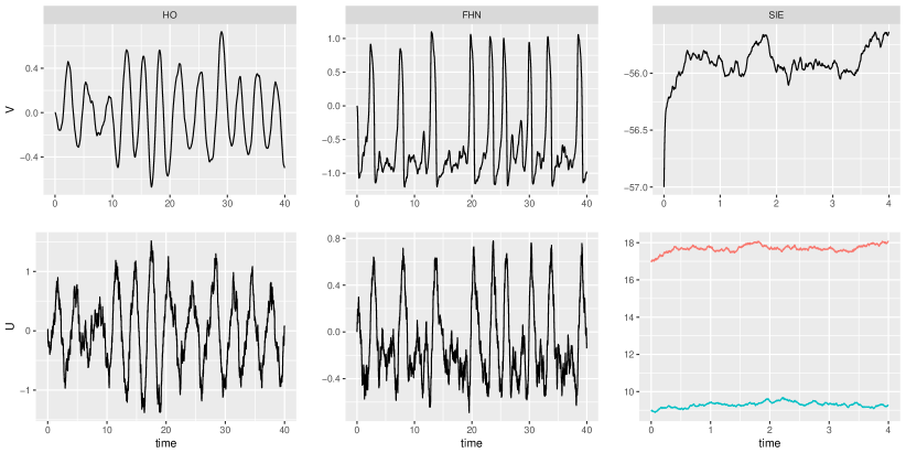
Figure 1: Simulated paths of the three example models. Left: Harmonic Oscillator. Middle: FitzHugh-Nagumo model. Right: Synaptic Inhibition and Excitation model. Upper plots: The smooth coordinate $V$. Lower plots: The rough coordinates $U$. The rough paths of the SIE model are excitatory (red) and inhibitory (green) conductances. Parameter values are given in Section 6.

To compare with the analysis of the other models, we make a Taylor expansion in $\Delta$ up to order 2 obtaining

$$\mathbb{E}(X_{t+\Delta}|X_{t}=x)=x+\Delta B_{\mbox{HO}}(x)+\mathcal{O}(\Delta^{3})$$ (20)

where

$$\Delta B_{\mbox{HO}}(x)=\Delta\left(\begin{array}[]{c}x_{2}-(Dx_{1}+\gamma x_{2})\frac{\Delta}{2}\\ -(Dx_{1}+\gamma x_{2})+(\gamma(Dx_{1}+\gamma x_{2})-Dx_{2})\frac{\Delta}{2}\end{array}\right).$$ (21)

Furthermore,

$$\mbox{Var}(X_{t+\Delta} |X_{t}=x)=\frac{\sigma^{2}}{2\gamma D}\left[\begin{array}[]{cc}1&0\\ 0&D\\ \end{array}\right]+$$ (24)

$$\frac{\sigma^{2}e^{-\gamma\Delta}}{4d^{2}}\left[\begin{array}[]{cc}\frac{2}{\gamma}\!-\!\frac{d}{D}\sinh\left(2d\Delta\right)\!-\!\frac{\gamma}{2D}\cosh\left(2d\Delta\right)&\cosh\left(2d\Delta\right)-1\\ \cosh\left(2d\Delta\right)-1&\frac{2D}{\gamma}\!+\!d\sinh\left(2d\Delta\right)\!-\!\frac{\gamma}{2}\cosh\left(2d\Delta\right)\\ \end{array}\right]$$ (27)

with Taylor expansion up to order 3 in $\Delta$

$$\mbox{Var}(X_{t+\Delta} |X_{t}=x)=\sigma^{2}\left[\begin{array}[]{cc}\frac{1}{3}\Delta^{3}&\frac{1}{2}\Delta^{2}-\frac{1}{2}\Delta^{3}\gamma\\ \frac{1}{2}\Delta^{2}-\frac{1}{2}\Delta^{3}\gamma&\Delta-\gamma\Delta^{2}+\frac{1}{3}\Delta^{3}(2\gamma^{2}-D)\\ \end{array}\right]+\mathcal{O}(\Delta^{4})$$ (30)

where we need a higher order for the variance for later convergence results, since otherwise the variance of the first coordinate is zero.

The invariant distribution is Gaussian,

$$X_{\infty}\sim\mathcal{N}\left(0,\frac{\sigma^{2}}{2\gamma D}\left[\begin{array}[]{cc}1&0\\ 0&D\\ \end{array}\right]\right).$$

The solution of this system has thus moments of any order. An example path can be found in Figure 1.

2.5.2 FitzHugh-Nagumo

A prototype of a model of a spiking neuron is the FitzHugh-Nagumo model, which is a minimal representation of more realistic neuron models, such as the Hodgkin-Huxley model, modelling the neuronal firing mechanisms (FitzHugh, 1961; Nagumo et al., 1962; Hodgkin & Huxley, 1952).

Consider the stochastic hypoelliptic FitzHugh-Nagumo model, defined as the solution to the system

$$\left\{\begin{array}[]{ccl}dV_{t}&=&\frac{1}{\varepsilon}(V_{t}-V_{t}^{3}-U_{t}+s)dt,\\ dU_{t}&=&\left(\gamma V_{t}-U_{t}+{\alpha}\right)dt+\sigma dB_{t},\end{array}\right.$$ (31)

where the variable $V_{t}$ represents the membrane potential of a neuron at time $t$, $U_{t}$ is a recovery variable, which could represent channel kinetics, and $p=1$.

Parameter $s$ is the magnitude of the stimulus current. When only $V_{t}$ is observed, $s$ is not identifiable (Jensen et al., 2012). Often $s$ represents injected current and is thus controlled in a given experiment, and it is therefore reasonable to assume it known, so that $\psi=\varepsilon$. Thus, parameters to be estimated are $\sigma,\psi=(\varepsilon)$ and $\varphi=(\gamma,{\alpha})$.

The distribution of $X_{t}=(V_{t},U_{t})^{T}$ is unknown, but moments can be approximated by using (11), where the generator of model (31) is

$$Lf(x) = \frac{1}{\varepsilon}(x_{1}-x_{1}^{3}-x_{2}+s)\frac{\partial f}{dx_{1}}+(\gamma x_{1}-x_{2}+{\alpha})\frac{\partial f}{dx_{2}}+\frac{1}{2}\sigma^{2}\frac{\partial^{2}f}{dx_{2}^{2}}.$$

We obtain

$$\mathbb{E}(X_{t+\Delta}|X_{t}=x)=x+\Delta B_{\mbox{FHN}}(x)+\mathcal{O}(\Delta^{3})$$

where

$$\Delta B_{\mbox{FHN}}(x)=$$ (32)

$$\Delta\left(\begin{array}[]{c}\frac{1}{\varepsilon}(x_{1}-x_{1}^{3}-x_{2}+s)+\displaystyle{\frac{\Delta}{2}}\frac{1}{\varepsilon}\left(\frac{1}{\varepsilon}(1-3x_{1}^{2})(x_{1}-x_{1}^{3}-x_{2}+s)-(\gamma x_{1}-x_{2}-{\alpha})\right)\\ (\gamma x_{1}-x_{2}+{\alpha})+\displaystyle{\frac{\Delta}{2}}\left(\frac{\gamma}{\varepsilon}(x_{1}-x_{1}^{3}-x_{2}+s)-(\gamma x_{1}-x_{2}+{\alpha})\right)\end{array}\!\!\right)$$ (35)

and

$$\mbox{Var}(X_{t+\Delta} |X_{t}=x)=\sigma^{2}\left[\begin{array}[]{cc}\frac{1}{3}\Delta^{3}\frac{1}{\varepsilon^{2}}{+\mathcal{O}(\Delta^{4})}&-\frac{1}{2}\Delta^{2}\frac{1}{\varepsilon}{+\mathcal{O}(\Delta^{3})\vspace{2mm}}\\ -\frac{1}{2}\Delta^{2}\frac{1}{\varepsilon}{+\mathcal{O}(\Delta^{3})}&\Delta-\Delta^{2}{+\mathcal{O}(\Delta^{3})}\\ \end{array}\right].$$ (38)

An example path can be found in Figure 1.

2.5.3 Synaptic-conductance model

A neuron, which reliably can be characterized as a single electrical compartment, and which receives excitatory and inhibitory synaptic bombardment, has a voltage dynamics across the membrane that can be described by this conductance-based model with diffusion synaptic input (Dayan & Abbott, 2001; Berg & Ditlevsen, 2013)

$$\left\{\begin{array}[]{ccl}CdV_{t}&=&(-G_{L}(V_{t}-V_{L})-G_{E,t}(V_{t}-V_{E})-G_{I,t}(V_{t}-V_{I})+I_{inj})dt\\[2.84526pt] dG_{E,t}&=&-\frac{1}{\tau_{E}}(G_{E,t}-\bar{g}_{E})dt+\sigma_{E}\sqrt{G_{E,t}}dB_{E,t}\\[2.84526pt] dG_{I,t}&=&-\frac{1}{\tau_{I}}(G_{I,t}-\bar{g}_{I})dt+\sigma_{I}\sqrt{G_{I,t}}dB_{I,t}\end{array}\right.$$ (39)

where $C$ is the total capacitance, $G_{L}$, $G_{E}$ and $G_{I}$ are the leak, excitation, and inhibition conductances, $V_{L}$, $V_{E}$ and $V_{I}$ are their respective reversal potentials, and $I_{inj}$ is the injected current. The conductances $G_{{E},t}$ and $G_{{I},t}$ are assumed to be stochastic functions of time, where $(B_{E,t})$ and $(B_{I,t})$ are two independent Brownian motions. The square roots in the diffusion coefficient ensures that the conductances stay positive. Parameters $\tau_{E},\tau_{I}$ are time constants, $\bar{g}_{E},\bar{g}_{I}$ the mean conductances, and $\sigma_{E},\sigma_{I}$ the diffusion coefficients, scaling the variability of these two processes. Here, $U_{t}=(G_{{E},t},G_{{I},t})^{T}$ and $p=2$. We assume the capacitance and the reversal potentials known, which are easily determined in independent experiments (Berg & Ditlevsen, 2013), as well as $I_{inj}$, which is controlled by the experimenter. Thus, the drift function $a$ does not depend on an unknown parameter, $\varphi=(\bar{g}_{E},\bar{g}_{I},\tau_{E},\tau_{I})$, and $\sigma=(\sigma_{E},\sigma_{I})$.

The distribution of $V_{t}$ is also unknown for this model, whereas $U_{t}$ are independent square root processes (also called CIR processes), which have transition densities following non-central chi-square distributions. However, for illustration of the methodology, we will approximate moments by using the generator of model (39),

$$Lf(x) = \frac{1}{C}(-G_{L}(x_{1}-V_{L})-x_{2}(x_{1}-V_{E})-x_{3}(x_{1}-V_{I})+I_{inj})\frac{\partial f}{dx_{1}}$$

$$-\frac{1}{\tau_{E}}(x_{2}-\bar{g}_{E})\frac{\partial f}{dx_{2}}-\frac{1}{\tau_{I}}(x_{3}-\bar{g}_{I})\frac{\partial f}{dx_{3}}+\frac{1}{2}\sigma_{E}^{2}x_{2}\frac{\partial^{2}f}{dx_{2}^{2}}+\frac{1}{2}\sigma_{I}^{2}x_{3}\frac{\partial^{2}f}{dx_{3}^{2}}$$

and equation (11). We obtain

$$\mathbb{E} (X_{t+\Delta})|X_{t}=x)=x+\Delta B_{\mbox{SIE}}(x)+\mathcal{O}(\Delta^{3})$$ (40)

where

$$\Delta B_{\mbox{SIE}}(x)\!=\!\Delta\!\left(\begin{array}[]{c}\!\!\!b_{1}(x)\displaystyle{-\frac{\Delta}{2C}}\!\left(b_{1}(x)(G_{L}\!+\!x_{2}\!+\!x_{3})\!+\!b_{2}(x)(x_{1}\!-\!V_{E})+b_{3}(x)(x_{1}\!-\!V_{I})\right)\\ b_{2}(x)-\displaystyle{\frac{\Delta}{2}}\left(b_{2}(x)\frac{1}{\tau_{E}}\right)\\ b_{3}(x)-\displaystyle{\frac{\Delta}{2}}\left(b_{3}(x)\frac{1}{\tau_{I}}\right)\end{array}\!\!\right)\!$$ (41)

and

$$\mbox{Var}(X_{t+\Delta}|X_{t}=x)=$$ (42)

$$\left[\begin{array}[]{ccc}\frac{\Delta^{3}}{3C^{2}}((x_{1}\!-\!V_{E})^{2}\sigma_{E}^{2}x_{2}\!+\!(x_{1}\!-\!V_{I})^{2}\sigma_{I}^{2}x_{3}){+\mathcal{O}(\Delta^{4})}&-\frac{\Delta^{2}}{2C}\sigma_{E}^{2}x_{2}(x_{1}-V_{E}){+\mathcal{O}(\Delta^{3})}&-\frac{\Delta^{2}}{2C}\sigma_{I}^{2}x_{3}(x_{1}-V_{I}){+\mathcal{O}(\Delta^{3})\vspace{2mm}}\\ -\frac{\Delta^{2}}{2C}\sigma_{E}^{2}x_{2}(x_{1}-V_{E}){+\mathcal{O}(\Delta^{3})}&\Delta\sigma_{E}^{2}x_{2}{+\mathcal{O}(\Delta^{2})}&0\vspace{2mm}\\ -\frac{\Delta^{2}}{2C}\sigma_{I}^{2}x_{3}(x_{1}-V_{I}){+\mathcal{O}(\Delta^{3})}&0&\Delta\sigma_{I}^{2}x_{3}{+\mathcal{O}(\Delta^{2})}\end{array}\right].$$ (46)

An example path can be found in Figure 1. The red path is the excitatory conductance, the green path is the inhibitory conductance.

3 Discretization scheme

The transition density for model (4) is generally unknown, and a possible approximation to the likelihood function is the likelihood for some approximating scheme of the discretized process $X_{0:n}$. We will write $\tilde{X}_{i}$ for the approximated process, or $\tilde{V}_{i}$ and $\tilde{U}_{i}$ where relevant.

The most commonly applied scheme to approximate the likelihood in SDEs, especially for high-frequency data, is the Euler-Maruyama approximation of model (4), which leads to a discretized model defined as follows

$$\tilde{V}_{i+1} = \tilde{V}_{i}+\Delta a(\tilde{V}_{i},\tilde{U}_{i}),$$ (47)

$$\tilde{U}_{i+1} = \tilde{U}_{i}+\Delta A(\tilde{V}_{i},\tilde{U}_{i})+\Gamma(\tilde{V}_{i},\tilde{U}_{i})\eta_{i},$$

where $(\eta_{i})$ are centered Gaussian vectors with variance $\Delta I_{p}$. Thus, the transition density of the approximate discretized scheme is a degenerate Gaussian distribution, since there is no stochastic term on the first coordinate. The same happens for the Milstein-scheme with strong order of convergence equal to 1.

3.1 Discretization with 1.5 scheme

We propose to use a higher order scheme, namely the 1.5 strong order scheme (Kloeden & Platen, 1992), using the hypoellipticity of (4) to propagate the noise into the first coordinate. For a diagonal diffusion matrix as in (6) the scheme is as follows, where for readability we have suppressed the dependence on $(V_{i},U_{i})$,

$$\tilde{V}_{i+1} = \tilde{V}_{i}+\Delta a+\frac{\Delta^{2}}{2}\partial_{x}a\,b+\frac{\Delta^{2}}{4}\bigtriangledown^{2}_{\bar{\Gamma}}a+\partial_{u}a\,\Gamma\xi_{i}$$ (48)

$$\tilde{U}_{i+1} = \tilde{U}_{i}+\Delta A+\frac{\Delta^{2}}{2}\partial_{x}A\,b+\frac{\Delta^{2}}{4}\bigtriangledown^{2}_{\bar{\Gamma}}A+\Gamma\eta_{i}+\partial_{u}A\,\Gamma\xi_{i}$$ (49)

$$+\frac{1}{2}\partial_{u}\bar{\Gamma}\,\Gamma(\eta_{i}^{*2}-{\Delta}\mathbf{1}_{p})+\partial_{u}\bar{\Gamma}\,A(\Delta\eta_{i}-\xi_{i})+\frac{1}{2}\bigtriangledown^{2}_{\bar{\Gamma}}\bar{\Gamma}(\Delta\eta_{i}-\xi_{i})$$

$$+\frac{1}{2}{\left(\left(\partial_{u}\bar{\Gamma}\right)^{2}\Gamma+\bigtriangledown^{2}_{\bar{\Gamma}}\bar{\Gamma}\right)}(\frac{1}{3}\eta_{i}\eta_{i}^{T}-\Delta I_{p})\eta_{i}$$

where $(\eta_{i})$ are centered Gaussian vectors with variance $\Delta I_{p}$, $(\xi_{i})$ are centered Gaussian vectors with variance $\Delta^{3}/3I_{p}$, Cov$(\eta_{i},\xi_{i})=\Delta^{2}/2I_{p}$ and Cov$(\eta_{i},\xi_{j})=0$ for $i\neq j$. Furthermore, $\eta_{i}^{*2}$ denotes the vector with the squared entries of $\eta_{i}$. Notice how noise of order $\Delta^{3/2}$ is now propagated into the first equation, since the last term on the right hand side of (48) is non-zero if condition (C1) is fulfilled. If $\Gamma$ is independent of the process (additive noise) then the last two lines in (49) are zero.

To simplify the notation later on, we rewrite equations (48)-(49) as

$$\left(\begin{array}[]{c}\tilde{V}_{i+1}\\ \tilde{U}_{i+1}\end{array}\right)=\left(\begin{array}[]{c}\tilde{V}_{i}\\ \tilde{U}_{i}\end{array}\right)+\Delta B(\tilde{V}_{i},\tilde{U}_{i})+\varepsilon_{i},\quad\varepsilon_{i}\sim\mathcal{N}_{p+1}(0,\Sigma(\tilde{V}_{i},\tilde{U}_{i}))$$ (50)

where $\Delta B(v,u)_{j}=\Delta b_{j}+\frac{\Delta^{2}}{2}\partial_{x}b_{j}\,b+\frac{\Delta^{2}}{4}\bigtriangledown^{2}_{\bar{\Gamma}}b_{j}$ is the scheme for the drift and $\Sigma(v,u)$ is the variance matrix of the scheme. Up to leading order, the variance matrix is given by

$$\Sigma(v,u)=\left(\begin{array}[]{cc}\partial_{u}a\,\Gamma\Gamma^{T}(\partial_{u}a)^{T}\frac{\Delta^{3}}{3}&\partial_{u}a\,\Gamma\Gamma^{T}\frac{\Delta^{2}}{2}\\ \Gamma\Gamma^{T}(\partial_{u}a)^{T}\frac{\Delta^{2}}{2}&\Gamma\Gamma^{T}\Delta\\ \end{array}\right).$$ (51)

Since the mean term coincides with the true mean up to order $\Delta^{2}$, see eqs. (13) and (14), the functions ${\Delta}B(v,u)$ for models (17), (31), and (39) are given in (21), (32) and (41), respectively. The variance matrix $\Sigma(\tilde{V}_{i},\tilde{U}_{i})$ of the above scheme for the three models (17), (31), and (39) are

$$\,\Sigma_{\mbox{HO}}\,\,=\sigma^{2}\left(\begin{array}[]{cc}\frac{1}{3}\Delta^{3}&\frac{1}{2}\Delta^{2}-\frac{1}{3}\Delta^{3}\gamma\\ \frac{1}{2}\Delta^{2}-\frac{1}{3}\Delta^{3}\gamma&\Delta-\Delta^{2}\gamma+\frac{1}{3}\Delta^{3}\gamma^{2}\\ \end{array}\right),$$ (54)

$$\Sigma_{\mbox{FHN}}=\sigma^{2}\left(\begin{array}[]{cc}\frac{1}{3}\Delta^{3}\varepsilon^{-2}&\left(-\frac{1}{2}\Delta^{2}+\frac{1}{3}\Delta^{3}\right)\varepsilon^{-1}\\ \left(-\frac{1}{2}\Delta^{2}+\frac{1}{3}\Delta^{3}\right)\varepsilon^{-1}&\Delta-\Delta^{2}+\frac{1}{3}\Delta^{3}\\ \end{array}\!\!\right),$$ (57)

$$\,\Sigma_{\mbox{SIE}}(\tilde{V}_{i},\tilde{U}_{i})\,\,=$$ (58)

$$\left(\begin{array}[]{ccc}\!\!\!\!\frac{\Delta^{3}}{3}\!\left({(\tilde{V}_{i}\!-\!V_{E})^{2}}\sigma^{2}_{E}\tilde{G}_{E,i}\!+\!{(\tilde{V}_{i}\!-\!V_{I})^{2}}\sigma^{2}_{I}\tilde{G}_{I,i}\right)&-\sigma^{2}_{E}{(\tilde{V}_{i}\!-\!V_{E})}\tilde{G}_{E,i}\!\left(\frac{\Delta^{2}}{2}\!\!+\!\frac{\Delta^{3}}{6\tau_{E}}\right)&-\sigma^{2}_{I}{(\tilde{V}_{i}\!-\!V_{I})}\tilde{G}_{I,i}\!\left(\frac{\Delta^{2}}{2}\!\!+\!\frac{\Delta^{3}}{6\tau_{I}}\right)\\ -\sigma^{2}_{E}{(\tilde{V}_{i}-V_{E})}\tilde{G}_{E,i}\!\left(\frac{\Delta^{2}}{2}\!\!+\!\frac{\Delta^{3}}{6\tau_{E}}\right)&\sigma^{2}_{E}\tilde{G}_{E,i}\left(\Delta-\frac{\Delta^{2}}{2\tau_{E}}+\frac{\Delta^{3}}{12\tau_{E}^{2}}\right)&0\\ -\sigma^{2}_{I}{(\tilde{V}_{i}-V_{I})}\tilde{G}_{I,i}\!\left(\frac{\Delta^{2}}{2}\!\!+\!\frac{\Delta^{3}}{6\tau_{I}}\right)&0&\sigma^{2}_{I}\tilde{G}_{I,i}\left(\Delta\!-\!\frac{\Delta^{2}}{2\tau_{I}}\!+\!\frac{\Delta^{3}}{12\tau_{I}^{2}}\right)\\ \end{array}\right).$$ (62)

For comparison, we recall the variance matrix for the HO model suggested by Pokern et al. (2009),

$$\,\Sigma_{\mbox{HO, Pokern}}\,\,=\sigma^{2}\left(\begin{array}[]{cc}\frac{1}{3}\Delta^{3}&\frac{1}{2}\Delta^{2}\\ \frac{1}{2}\Delta^{2}&\Delta\\ \end{array}\right),$$ (65)

which coincides with (54) up to lowest order at each matrix entry. Furthermore, it coincides with (51) when $p=1,a(v,u)=u$ and $\Gamma(v,u)=\sigma$.

3.2 Remarks on the convergence of the scheme

The scheme (48)–(49) has a strong order 1.5 and a weak order 2 convergence (Kloeden & Platen, 1992). The following bounds follow by comparing eqs. (11)–(16) with eqs. (48)–(49). These bounds are needed later to prove consistency.

Proposition 1

[Moment bounds]

$$\mathbb{E}(V_{i+1}-V_{i}-\Delta B(X_{i})_{1}|X_{i}{=x}) =\mathcal{O}(\Delta^{3})$$

$$\mathbb{E}(U_{i+1}-U_{i}-\Delta B(X_{i})_{(-1)}|X_{i}{=x}) =\mathcal{O}(\Delta^{3})$$

$$\mathbb{E}((V_{i+1}-V_{i}-\Delta B(X_{i})_{1})^{2}|X_{i}{=x}) =\frac{\Delta^{3}}{3}\partial_{u}a\Gamma\Gamma^{T}(\partial_{u}a)^{T}+\mathcal{O}(\Delta^{4})$$

$$\mathbb{E}((U_{i+1}\!-\!U_{i}\!-\!\Delta B(X_{i})_{(-1)})(U_{i+1}\!-\!U_{i}\!-\!\Delta B(X_{i})_{(-1)})^{T}|X_{i}{=x}) =\Delta\Gamma\Gamma^{T}+\mathcal{O}(\Delta^{2})$$

$$\mathbb{E}((V_{i+1}-V_{i}-\Delta B(X_{i})_{1})^{4}|X_{i}{=x}) =\mathcal{O}(\Delta^{4})$$

$$\mathbb{E}(((U_{i+1}\!-\!U_{i}\!-\!\Delta B(X_{i})_{(-1)})(U_{i+1}\!-\!U_{i}\!-\!\Delta B(X_{i})_{(-1)})^{T})^{2}|X_{i}{=x}) =\mathcal{O}(\Delta^{2})$$

where $B(X_{i})_{(-1)}$ denotes the vector $B(X_{i})$ with the first coordinate omitted.

Note that the expected value of the difference between the true drift and the approximating drift $\Delta B$ is of order $\Delta^{3}$, because of the higher order scheme. This is necessary for the later convergence results in Propositions 2 and 3, in particular, the technical lemmas of Section 7.1.

Another useful convergence result is the convergence of the transition density of the scheme to the exact transition density, as proved in the elliptic case by Bally & Talay (1996) under smooth conditions on the drift functions and diffusion coefficients. Unfortunately, this result is much more difficult to obtain for a hypoelliptic SDE such as system (4). This is beyond the scope of this paper.

4 Complete observations

In this Section we investigate parameter estimation when all coordinates are discretely observed. Later, we extend to the situation where only the first coordinate is observed.

4.1 Contrast estimator

The goal is to estimate the parameter $\theta=(\psi,\varphi,\sigma)$ by maximum likelihood of the approximate model, with complete likelihood

$$p_{\Delta}(V_{0:n},U_{0:n};\theta)=p(V_{0},U_{0};\theta)\prod_{i=1}^{n}p_{\Delta}(V_{i},U_{i}|V_{i-1},U_{i-1};\theta),$$ (66)

where $p(V_{0},U_{0};\theta)$ is the density of the initial value of the process. The contribution from this single data point is negligible for relevant sample sizes, and we will simply assume it degenerate in the observed value $(V_{0},U_{0})$. This likelihood corresponds to a pseudo-likelihood for the exact diffusion, with exact complete likelihood given in (7). The estimator is then the minimizer of minus 2 times the log complete likelihood:

$$\arg\min_{\theta} \sum_{i=0}^{n-1}\left((X_{i+1}\!-\!X_{i}-\Delta B(X_{i};\theta))^{T}\,\Sigma_{i}^{-1}(X_{i+1}\!-\!X_{i}-\Delta B(X_{i};\theta))+\log\det(\Sigma_{i})\right)$$ (67)

This criterion is ill behaved because the system is hypoelliptic, so the order of the variance for $V$ is $\Delta^{3}$ and for $U$ it is $\Delta$. Therefore, we propose to separate the estimation of parameter $\psi$ of the first coordinate from parameters $(\phi,\sigma)$ of the second coordinate.

We thus introduce two new contrasts and their corresponding estimators.

Definition 1

The estimator of the parameters of the first coordinate is given by

$$\hat{\psi}_{n} = \arg\min_{\psi}\left(\frac{3}{\Delta^{3}}\sum_{i=0}^{n-1}\frac{(V_{i+1}-V_{i}-\Delta B(X_{i};\theta)_{1})^{2}}{(\partial_{u}a(X_{i};\psi))\Gamma\Gamma^{T}(X_{i};\sigma)(\partial_{u}a(X_{i};\psi))^{T}}\right.$$

$$\left.+\sum_{i=0}^{n-1}\log((\partial_{u}a(X_{i};\psi))\Gamma\Gamma^{T}(X_{i};\sigma)(\partial_{u}a(X_{i};\psi))^{T})\right)$$

where the parameters $\varphi$ and $\sigma$ are fixed.

The estimator of the parameters of the second coordinate is given by

$$(\hat{\varphi}_{n},\hat{\sigma}_{n}^{2}) = \arg\min_{\varphi,\sigma^{2}}\left(\sum_{i=0}^{n-1}\log(\det(\Gamma\Gamma^{T}(X_{i};\sigma))\right.$$

$$+ \left.\sum_{i=0}^{n-1}(U_{i+1}\!-\!U_{i}\!-\Delta B(X_{i};\theta)_{(-1)})^{T}\left(\Delta\Gamma\Gamma^{T}\!(X_{i};\sigma)\right)^{-1}\!(U_{i+1}\!-\!U_{i}\!-\Delta B(X_{i};\theta)_{(-1)})\right)$$

where the parameter $\psi$ is fixed.

The first contrast corresponds to the pseudo-likelihood of the marginal distribution of the first coordinate. The second contrast is a simplification of the pseudo-likelihood of the marginal of the coordinates with direct noise: the variance appearing in the pseudo-likelihood is $\Delta\Gamma\Gamma^{T}(X_{i},\sigma)(1+o(\Delta))$ and is simplified to $\Delta\Gamma\Gamma^{T}(X_{i},\sigma)$ in the contrast (1), since the variance is dominated by the lowest order term. The contrasts (1) and (1) require the other parameters to be fixed. To estimate the complete parameter vector, the parameters are initialized and then the optimization procedure iterates between the two estimators (1) and (1). The numerical optimization of the criteria is not sensitive to those fixed values since they appear in higher order terms.

4.2 Theoretical properties of the contrast estimators

We start by proving the consistency of the contrast estimators. The asymptotics are in number of observations $n$ and length of time step between observations $\Delta_{n}$, where we have introduced an index $n$ to clarify the relevant asymptotics.

Proposition 2

Assume the drift function $a$ can be decomposed as either: $a(x;\psi)=a_{v}(v,\psi)+a_{u}(u)$ or $a(x;\psi)=a_{v}(v)+\psi a_{u}(x)$. Denote by $\psi_{0}$ the true value of the parameter, and assume $(\varphi,\sigma^{2})$ known. If $\Delta_{n}\rightarrow 0$ and $n\Delta_{n}\rightarrow\infty$ then

$$\hat{\psi}_{n}\stackrel{{\scriptstyle P}}{{\rightarrow}}\psi_{0}.$$

Proposition 3

Denote by $(\varphi_{0},\sigma^{2}_{0})$ the true values of the parameters, and assume $\psi$ known. If $\Delta_{n}\rightarrow 0$ and $n\Delta_{n}\rightarrow\infty$ then

$$(\hat{\varphi}_{n},\hat{\sigma}^{2}_{n})\stackrel{{\scriptstyle P}}{{\rightarrow}}(\varphi_{0},\sigma^{2}_{0}).$$

The proofs are given in Supplementary Material, Section 7. In the numerical examples, the parameters are estimated and not fixed to their true values.

The convergence conditions are standard: the length of the observation interval has to increase for consistency of drift parameters. For consistency of the variance parameter, it can be proven that only $\Delta_{n}\rightarrow 0$ and $n\rightarrow\infty$ are needed, but we will not pursue that here.

The estimators are asymptotically normal. We prove the result for $(\hat{\varphi}_{n},\hat{\sigma}^{2}_{n})$ and give some partial proofs for $\hat{\psi}_{n}$.

Theorem 1

Let $\nu(\cdot)$ denote the stationary density of model (4). If $\Delta_{n}\rightarrow 0$, $n\Delta_{n}\rightarrow\infty$ and $n\Delta_{n}^{2}\rightarrow 0$, then

$$\sqrt{n\Delta_{n}}(\hat{\varphi}_{n}-\varphi_{0}) \stackrel{{\scriptstyle\mathcal{D}}}{{\rightarrow}} \mathcal{N}\left(0,\left(\nu\left((\partial_{\varphi}A(\cdot,\varphi_{0}))^{T}(\Gamma\Gamma^{T}(\cdot,\sigma_{0}))^{-1}(\partial_{\varphi}A(\cdot,\varphi_{0}))\right)\right)^{-1}\right)$$

$$\sqrt{n}(\hat{\sigma}_{n}-\sigma_{0}) \stackrel{{\scriptstyle\mathcal{D}}}{{\rightarrow}} \mathcal{N}\left(0,2\left(\nu\left((\partial_{\sigma}\Gamma\Gamma^{T}(\cdot,\varphi_{0}))^{T}(\Gamma\Gamma^{T}(\cdot,\sigma_{0}))^{-1}(\partial_{\sigma}\Gamma\Gamma^{T}(\cdot,\varphi_{0}))\right)\right)^{2}\right)$$

where $\nu(f(\cdot))=\int f(x)d\nu(x)$.

For the estimator of the parameters of the smooth coordinate, the rate of convergence is faster.

Theorem 2

Let $\nu(\cdot)$ denote the stationary density of model (4). Assume the drift function $a$ can be decomposed as either: $a(x;\psi)=a_{v}(v,\psi)+a_{u}(u)$ or $a(x;\psi)=a_{v}(v)+\psi a_{u}(x)$. If $\Delta_{n}\rightarrow 0$, $n\Delta_{n}\rightarrow\infty$ and $n\Delta_{n}^{2}\rightarrow 0$, then

$$\sqrt{\frac{n}{\Delta_{n}}}(\hat{\psi}_{n}-\psi_{0}) \stackrel{{\scriptstyle\mathcal{D}}}{{\rightarrow}} \mathcal{N}\left(0,\frac{1}{3}\left(\nu\left((\partial_{\psi}a(\cdot,\psi_{0}))^{T}(\partial_{u}a(\cdot,\psi_{0})\Gamma\Gamma^{T}(\cdot,\sigma_{0})(\partial_{u}a(\cdot,\psi_{0}))^{T})^{-1}(\partial_{\psi}a(\cdot,{\psi_{0}}))\right)\right)^{-1}\right)$$

The proofs are given in Supplementary Material, Section 7.

5 Partial observations

In this Section we assume that we do not observe the coordinates $U_{t}$, which is the most relevant case for applications. The likelihood to maximize is therefore not the complete approximate likelihood, but the approximate likelihood $p_{\Delta}(V_{0:n};\theta)$ defined as the integral of the complete approximate likelihood (66) with respect to the hidden components.

$$p_{\Delta}(V_{0:n};\theta)=\int\prod_{i=1}^{n}p_{\Delta}(X_{i}|X_{i-1};\theta)dU_{0:n}.$$ (70)

It corresponds to a discretization of the exact likelihood (8).

The multiple integrals of equation (70) are difficult to handle and it is not possible to maximize the pseudo-likelihood directly. As explained in Section 4, it is easier to maximize the complete approximate likelihood, after imputing the hidden coordinates.

For models where $a(v,u)=a_{v}(v)+a_{u}(v)u$ for some functions $a_{v}$ and $a_{u}$ that do not depend on the parameter, such as in the HO model, the imputation is intuitive: the unobserved coordinate $U_{t}$ can be approximated by the differences of the observed coordinate $V_{t}$, $U_{i}\approx((V_{i+1}-V_{i})/\Delta-a_{v}(V_{i}))/a_{u}(V_{i})$. However, this induces a bias in the estimation of $\sigma$ (see Samson & Thieullen, 2012, for more details), and is moreover only applicable for drift functions of the observed coordinate such that $u$ can be isolated. We will take advantage of that when initializing the estimation algorithm in Section 5.3.

In this paper we propose to use a particle filter, also known as Sequential Monte Carlo (SMC), to impute the hidden coordinates. Then, this imputed path is plugged into a stochastic SAEM algorithm (Delyon et al., 1999), as done in Ditlevsen & Samson (2014) for the elliptic case. The SMC proposed by Ditlevsen & Samson (2014) allows to filter a hidden coordinate that is not autonomous in the sense that the equation for $U_{t}$ depends on the first coordinate $V_{t}$. Here, we extend the algorithm to the case of $p$ hidden coordinates, to deal with a $p+1$-dimensional SDE.

More precisely, the observable vector $V_{0:n}$ is then part of a so-called complete vector $(V_{0:n},U_{0:n})$, where $U_{0:n}$ has to be imputed. At each iteration of the SAEM algorithm, the unobserved data are filtered under the smoothing distribution $p_{\Delta}(U_{0:n}\;|V_{0:n};\theta)$ with an SMC. Then the parameters are updated using the pseudo-likelihood proposed in Section 4. Details on the filtering are given in Section 5.1, and the SAEM algorithm is presented in Section 5.2.

5.1 Particle filter

The SMC proposed in Ditlevsen & Samson (2014) is designed for a $p=1$-dimensional hidden coordinate. Here we extend to the general case. For notational simplicity, $\theta$ is omitted in the rest of this Section.

The SMC algorithm provides $K$ particles $(U^{(k)}_{0:n})_{k=1,\dots,K}$ and weights $(W^{(k)}_{0:n})_{k=1,\dots,K}$ such that the empirical measure $\Psi^{K}_{n}=\sum_{k=1}^{K}W_{n}(U_{0:n}^{(k)})\mathbf{1}_{U_{0:n}^{(k)}}$ approximates the conditional smoothing distribution $p_{\Delta}(U_{0:n}|V_{0:n})$ (Doucet et al., 2001). The SMC method relies on proposal distributions $q(U_{i}|V_{i},V_{i-1},U_{i-1})$ to sample the particles from these distributions. We write $V_{0:i}=(V_{0},\ldots,V_{i})$ and likewise for $U_{0:i}$.

Algorithm 1 (SMC algorithm)

 

• At time $i=0$: $\forall\,k=1,\ldots,K$

  1. sample $U_{0}^{(k)}$ from $p(U_{0}|V_{0})$

  2. compute and normalize the weights:
     $w_{0}\left(U^{(k)}_{0}\right)={1}$, $\quad W_{0}\left(U^{(k)}_{0}\right)=\frac{w_{0}\left(U^{(k)}_{0}\right)}{\sum_{k=1}^{K}w_{0}\left(U^{(k)}_{0}\right)}$

• At time $i=1,\ldots,n$: $\forall\,k=1,\ldots,K$

  1. sample indices $A_{i-1}^{(k)}\sim r(\cdot|W_{i-1}(U_{0:i-1}^{(1)}),\ldots,W_{i-1}(U_{0:i-1}^{(K)}))$ where $r(\cdot)$ denotes the multinomial distribution and set
     $U_{0:i-1}^{{}^{\prime}(k)}=U_{0:i-1}^{(A_{i-1}^{(k)})}$

  2. sample $U^{(k)}_{i}\sim q\left(\cdot|V_{i-1:i},U^{{}^{\prime}(k)}_{i-1}\right)$ and set $U^{(k)}_{0:i}=(U_{0:i-1}^{{}^{\prime}(k)},U^{(k)}_{i})$

  3. compute and normalize the weights $W_{i}(U^{(k)}_{0:i})=\frac{w_{i}\left(U^{(k)}_{0:i}\right)}{\sum_{k=1}^{K}w_{i}\left(U^{(k)}_{0:i}\right)}$ with
     $w_{i}\left(U^{(k)}_{0:i}\right)=\frac{p_{\Delta}\left(V_{0:i},U^{(k)}_{0:i}\right)}{p_{\Delta}\left(V_{0:i-1},U_{0:i-1}^{{}^{\prime}(k)}\right)q\left(U^{(k)}_{i}|V_{i-1:i},U_{0:i-1}^{{}^{\prime}(k)}\right)}$

Natural choices for the proposal $q$ are either the transition density $q(U_{i}|V_{i-1:i},U_{i-1})=p_{\Delta}(U_{i}|V_{i-1},U_{i-1})$ or the conditional distribution $q(U_{i}|V_{i-1:i},U_{i-1})=p_{\Delta}(U_{i}|V_{i-1:i},U_{i-1})$, following Ditlevsen & Samson (2014). The two choices are not equivalent in the hypoelliptic case because the covariance matrix of the approximate scheme is not diagonal. The conditional distribution gives better results in practice and is used in the simulations. This is due to the extra information provided by also conditioning on $V_{i}$.

In the following, we present some asymptotic convergence results on the SMC algorithm. The assumptions can be found in Supplementary Material, Section 8.2. For a bounded Borel function $f$, denote $\Psi_{n}^{K}{(f)}=\sum_{k=1}^{K}f(U_{n}^{(k)})W_{n}(U_{0:n}^{(k)})$, the conditional expectation of $f$ under the empirical measure $\Psi_{n}^{K}$. We also denote $\pi_{n,\Delta}{(f)}=\mathbb{E}_{\Delta}\left(f(U_{n})|V_{0:n}\right)$ the conditional expectation under the smoothing distribution $p_{\Delta}(U_{0:n}|V_{0:n})$ of the approximate model.

Proposition 4

Under assumption (SMC3), for any $\varepsilon>0$, and for any bounded Borel function $f$ on $\mathbb{R}$, there exist constants $C_{1,\Delta}$ and $C_{2,\Delta}$ that do not depend on $K$, such that

$$\mathbb{P}\left(\left|\Psi_{n}^{K}{(f)}-\pi_{n,\Delta}{(f)}\right|\geq\varepsilon\right) \leq C_{1,\Delta}\exp\left(-K\frac{\varepsilon^{2}}{C_{2,\Delta}\|f\|^{2}}\right)$$ (71)

where $\|f\|$ is the sup-norm of $f$ and $C_{1,\Delta}$, $C_{2,\Delta}$ are constants detailed in Ditlevsen & Samson (2014).

The proof is the same as in Ditlevsen & Samson (2014). The hypoellipticity of the process is not a problem as the filter is applied on the discretized process where the noise has been propagated to the first coordinate, such that the ratio in Algorithm 1, step (c) will be well-defined when calculating the weights, since then $p_{\Delta}$ and $q$ are non-degenerate normal densities different from 0.

5.2 SAEM

The estimation method is based on a stochastic version of the EM algorithm (Dempster et al., 1977), namely the SAEM algorithm (Delyon et al., 1999) coupled to the SMC algorithm, as already proposed by Ditlevsen & Samson (2014) in the elliptic case. To fulfill convergence conditions of the algorithm, we consider the particular case of a distribution from an exponential family. Note that it is the discrete pseudo-likelihood (66) using the strong order 1.5 scheme that needs to fulfill the conditions. More precisely, we assume:

• The parameter space $\Theta$ is an open subset of $\mathbb{R}^{p}$. The complete pseudo-likelihood belongs to a curved exponential family, i.e., $\log p_{\Delta}(V_{0:n},U_{0:n};\theta)=-\psi(\theta)+\left\langle S(V_{0:n},U_{0:n}),\nu(\theta)\right\rangle$, where $\psi$ and $\nu$ are two functions of $\theta$, $S(V_{0:n},U_{0:n})$ is known as the minimal sufficient statistic of the complete model, taking its value in a subset ${\mathcal{S}}$ of $\mathbb{R}^{d}$, and $\left\langle\cdot,\cdot\right\rangle$ is the scalar product on $\mathbb{R}^{d}$.

The three models considered in this paper satisfy this assumption. Details of the sufficient statistic $S$ for the HO model are given in the Supplementary Material, Appendix 8.3.

Under assumption (M1), introducing a sequence of positive numbers $(a_{m})_{m\in\mathbb{N}}$ decreasing to zero, the SAEM-SMC algorithm is defined as follows.

Algorithm 2 (SAEM-SMC algorithm)

 

• Iteration $0$: initialization of $\;\widehat{\theta}_{0}$ and set $s_{0}=0$.

• Iteration $m\geq 1$:

  • simulation of the non-observed data $(U_{0:n}^{(m)})$ with SMC targeting the smoothing distribution $p_{\Delta}(U_{0:n}|V_{0:n};\widehat{\theta}_{m-1})$.

  • update $s_{m-1}$ using the stochastic approximation:

    $$s_{m}=s_{m-1}+a_{m-1}\left[S(V_{0:n},U_{0:n}^{(m)})-s_{m-1}\right]$$ (72)

  • update of $\widehat{\theta}_{m}$ by $\widehat{\theta}_{m}=\underset{\theta\in\Theta}{\arg\max}\left(-\psi(\theta)+\langle s_{m},\nu(\theta)\rangle\right).$

Simulation under the smoothing distribution can be performed using a naive forward approach, which amounts to carry forward trajectories in the particle filter. We also implemented a backward SMC smoother, with variance $O(n)$ instead of $O(n^{2})$ for the naive smoother. However, in practice, the stochastic averaging of the SA step reduces the variance by averaging over all the previous iterations using the step size $a_{m}$.

Following Ditlevsen & Samson (2014), we can prove the convergence of the SAEM-SMC algorithm, under standard assumptions that are recalled in the Supplementary Material, Section 8.2.

Theorem 3

Assume that (M1)-(M5), (SAEM1)-(SAEM3), and (SMC1)-(SMC3) hold. Then, with probability 1, $\lim_{m\rightarrow\infty}$ $d(\widehat{\theta}_{m},\mathcal{L})=0$ where $\mathcal{L}=\{\theta\in\Theta,\partial_{\theta}\ell_{\Delta}(\theta)=0\}$ is the set of stationary points of the log-likelihood $\ell_{\Delta}(\theta)=\log p_{\Delta}(V_{0:n};\theta)$.

Moreover, under assumptions (LOC1)-(LOC3) given in Delyon et al. (1999) on the regularity of the log-likelihood, the sequence $\widehat{\theta}_{m}$ converges with probability 1 to a (local) maximum of the likelihood $p_{\Delta}(V_{0:n};\theta)$.

The classical assumptions (M1)-(M5) are usually satisfied. Assumption (SAEM1) is easily satisfied by choosing properly the sequence $(a_{m})$. Assumptions (SAEM2) and (SAEM3) depend on the regularity of the model. They are satisfied for the 3 approximate models.

5.3 Initializing the algorithm

The SAEM algorithm requires initial values of $\theta$ to start. We detail our strategy to find initial values for the two first models. The SIE model is arbitrarily initialized with unknown parameters fixed at values of the correct order of magnitude.

For the HO model, we run the two-dimensional contrast based on complete observations of the two coordinates. As the $U$ coordinate is not observed, we replace it by the increments of $V$: $\tilde{U}_{i}=(V_{i+1}-V_{i})/\Delta$. Then the two-dimensional criterion is minimized and initial values $\hat{D}_{0},\hat{\gamma}_{0},\tilde{\sigma}_{0}$ are obtained. The value $\tilde{\sigma}_{0}$ is biased due to the approximation of $U_{i}$, as shown by Samson & Thieullen (2012). Therefore, we apply the bias correction suggested by Samson & Thieullen (2012) and use $\hat{\sigma}_{0}=\sqrt{\frac{3}{2}}\tilde{\sigma}_{0}$ as initial value.

For the FHN model, the problem is more difficult because the unknown parameter $\varepsilon$ appears in the equation of the observed coordinate. We fix an arbitrary value for $\hat{\varepsilon}_{0}$. Then we replace the hidden coordinate $U_{i}$ by $\tilde{U}_{i}=V_{i}-V_{i}^{3}+s-\hat{\varepsilon}_{0}\frac{V_{i+1}-V_{i}}{\Delta}$. Using $(V_{i},\tilde{U}_{i})$, we minimize the two-dimensional contrast to obtain initial values $\hat{\gamma}_{0},{\hat{\alpha}_{0}},\hat{\varepsilon}_{0}$.

6 Simulation study

6.1 Harmonic Oscillator

Parameter values of the Harmonic Oscillator used in the simulations are the same as those of Pokern et al. (2009); Samson & Thieullen (2012). The values are: $D=4$, $\gamma=0.5$, $\sigma=0.5$. Trajectories are simulated with the exact distribution eqs. (18)–(19)–(24) with time step $\Delta=0.02$ and $n=1000$ points. Then $\theta$ is estimated on each simulated trajectory. A hundred repetitions are used to evaluate the performance of the estimators.

The Particle filter aims at filtering the hidden process $(U_{t})$ from the observed process $(V_{t})$. We illustrate its performance on a simulated trajectory, with $\theta$ fixed at its true value. The SMC Particle filter algorithm is implemented with $K=100$ particles and the conditional transition density as proposal.

The performance of the SAEM-SMC algorithm is illustrated on 100 simulated trajectories. The SAEM algorithm is implemented with $m=80$ iterations and a sequence ($a_{m}$) equal to 1 during the 30 first iterations and equal to $a_{m}=1/(m-30)^{0.9}$ for $m>30$. The SMC algorithm is implemented with $K(m)=100$ particles at each iteration of the SAEM algorithm. The SAEM algorithm is initialized automatically by maximizing the log likelihood of the complete data, replacing the hidden $(U_{i\Delta})$ by the differences $((V_{(i+1)\Delta}-V_{i\Delta})/\Delta)$.

Several estimators are compared. The complete observation case is illustrated with the new contrast estimator (numerical optimisation of contrast (1)) and the Euler contrast from Samson & Thieullen (2012) (explicit estimators). The partial observation case is illustrated with the SAEM estimator and the Euler contrast from Samson & Thieullen (2012). Bayesian results from the weak order 1.5 scheme presented in Pokern et al. (2009) are also recalled, even if they are obtained with a different sampling ($n=10000$ and $\Delta=0.01$). This estimator is known from Pokern et al. (2009) to be biased. Results are given in Table 1.

Table 1: Harmonic Oscillator, mean and standard deviation (in parentheses) of estimators calculated from 100 trajectories with $\Delta=0.02$ and $n=1\,000$. Five estimation methods. Complete observations: new contrast estimator given in eq. (1) and Euler contrast from Samson & Thieullen (2012). Partial observations: SAEM, Euler contrast from Samson & Thieullen (2012) and weak order 1.5 estimator from Pokern et al. (2009) obtained with $n=10\,000$ and $\Delta=0.01$ (only the mean values for $D$ and $\gamma$ are given in their paper).

		Observations
		Complete		Partial
	True	New Contrast	Euler Contrast	SAEM	Euler Contrast	weak order 1.5
$D$	4.0	3.712 (0.634)	3.969 (0.540)	4.081 (0.503)	3.969 (0.540)	1.099 (–)
$\gamma$	0.5	0.701 (0.287)	0.716 (0.273)	0.663 (0.273)	0.754 (0.278)	0.139 (–)
$\sigma$	0.5	0.496 (0.014)	0.496 (0.011)	0.509 (0.012)	0.503 (0.011)	– (–)

The first four estimators give overall acceptable results, while the weak order 1.5 estimator of Pokern et al. (2009) is seriously biased. The best results are obtained with the SAEM. It might seem surprising that the SAEM performs even better than the estimators based on complete observations. This is due to the sensitivity of the numerical optimisation of the contrast (1) to the initial conditions for the iterative procedure, that were set to ${(\hat{\gamma}_{0},\hat{D}_{0},\hat{\sigma}_{0})=}(3,1,1)$. The stochasticity of the SAEM algorithm helps to avoid local optimization points, while the numerical optimizer might get stuck in some local minimum. The optimization of the Euler contrast is explicit for the HO model, and there is thus no dependence on initial conditions. It therefore outperforms the new contrast for $D$.

Comparing the SAEM and the Euler contrast for the partial observation case, they give results of the same order, even if slightly better for the SAEM. However, the SAEM is much more time consuming. Note also that the SAEM algorithm provides confidence intervals easily, which is not possible with the contrast estimators.

6.2 FitzHugh-Nagumo model

Parameter values of the FitzHugh-Nagumo model used in the simulations are : $\varepsilon=0.1$, $s=0$, $\gamma=1.5$, ${\alpha}=0.8$, $\sigma=0.3$. Trajectories are simulated with time step $\delta=0.002$ and $n=1000$ points are subsampled with observation time step $\Delta=10\delta$. Then $\theta$ is estimated on each simulated trajectory. A hundred repetitions are used to evaluate the performance of the estimators.

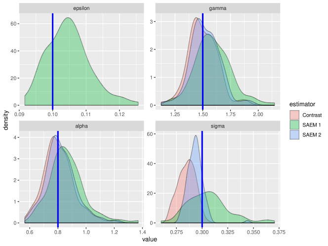
Figure 2: FHN estimation results for partial observations. Densities of estimated parameters over 100 repetitions for the new contrast method assuming $\varepsilon$ known (red), SAEM assuming $\varepsilon$ known (blue), SAEM estimating $\varepsilon$ (green). The blue vertical lines are the true values.

Several estimators are compared. First note that $\varepsilon$ is difficult to estimate because it appears in the first coordinate. Therefore, we first fix it at its true value. This allows to transform the system into a Langevin equation with $dV_{t}=Z_{t}dt$, and to apply the Euler contrast proposed by Samson & Thieullen (2012). With $\varepsilon$ fixed, we compare in the complete observation case the contrast estimator (numerical optimisation of contrast (1)) and the Euler contrast from Samson & Thieullen (2012) (explicit estimators). We also include the estimation of the full parameter vector by the new contrast given in eqs. (1) and (1). In the partial observation case we compare the SAEM estimator, the new contrast and the Euler contrast from Samson & Thieullen (2012). We also run the SAEM algorithm where $\varepsilon$ is not fixed but estimated.

The SAEM algorithm is implemented with $m=350$ iterations and a sequence ($a_{m}$) equal to 1 during the 250 first iterations and equal to $a_{m}=1/(m-250)^{0.9}$ for $m>250$. The SMC algorithm is implemented with $K=100$ particles at each SAEM iteration. The SAEM algorithm is initialized automatically by maximizing the log likelihood of the complete data, replacing the hidden $(U_{i\Delta})$ by the differences $(V_{i\Delta}-V_{i\Delta}^{3}s-\varepsilon(V_{(i+1)\Delta}-V_{i\Delta}))/\Delta$, $\varepsilon$ being initialized at ${\hat{\varepsilon}_{0}=}0.12$. Results are given in Table 2, and densities of estimates in the partially observed case are presented in Figure 2.

Table 2: FitzHugh-Nagumo model. Mean and standard deviation (in parentheses) of estimators calculated from 100 trajectories with $\Delta=0.02$ and $n=1\,000$. Seven estimation methods. Complete observations, $\varepsilon$ fixed: new contrast estimator and Euler contrast from Samson & Thieullen (2012). Complete observations, $\varepsilon$ estimated: new contrast estimator. Partial observations, $\varepsilon$ fixed: SAEM, new contrast and Euler contrast from Samson & Thieullen (2012) $\varepsilon$ fixed. Partial observations, $\varepsilon$ estimated. SAEM.

		Complete observations
		$\varepsilon$ fixed	$\varepsilon$ fixed	$\varepsilon$ estimated
	True	New Contrast	Euler Contrast	New Contrast
$\varepsilon$	0.1	–	–	0.101 (0.0005)
$\gamma$	1.5	1.412 (0.221)	1.363 (0.201)	1.516 (0.149)
${\alpha}$	0.8	0.826 (0.146)	0.756 (0.131)	0.822 (0.131)
$\sigma$	0.3	0.303 (0.014)	0.338 (0.024)	0.299 (0.007)
		Partial observations
		$\varepsilon$ fixed	$\varepsilon$ fixed	$\varepsilon$ fixed	$\varepsilon$ estimated
	True	SAEM	New Contrast	Euler Contrast	SAEM
$\varepsilon$	0.1	–	–	–	0.105 (0.006)
$\gamma$	1.5	1.523 (0.130)	1.512 (0.129)	1.500 (0.130)	1.592 (0.165)
${\alpha}$	0.8	0.822 (0.110)	0.815 (0.110)	0.807 (0.109)	0.865 (0.129)
$\sigma$	0.3	0.293 (0.008)	0.300 (0.023)	0.285 (0.008)	0.306 (0.021)

The results are acceptable overall. In the complete observation case, the new contrast gives better results than the Euler contrast. This is expected because the new constrast has a higher order of convergence. For the partial observation case, when $\varepsilon$ is fixed, the performance of the SAEM and the contrast are close. The Euler contrast gives better results with partial observations than complete observations (except for $\sigma$). This might be due to the sensitivity of the numerical optimization used to minimize the criteria. Finally, the SAEM gives good results when $\varepsilon$ is estimated, and this is the only method that can estimate it.

6.3 Synaptic-conductance model

Parameter values of the SIE model used in the simulations are : $G_{L}=50$, $V_{L}=-70$, $V_{E}=0$, $V_{I}=-80$, $I_{{inj}}=-60$, $\tau_{E}=0.5$, $\tau_{I}=1$, $\bar{g}_{E}=17.8$, $\bar{g}_{I}=9.4$, $\sigma_{E}=0.1$, $\sigma_{I}=0.1$. Initial conditions of the system are $V_{0}=-60$, $G_{e,0}=10$, $G_{i,0}=1$.

Trajectories are simulated with time step $\delta=0.002$ and $n=1000$ points are subsampled with observation time step $\Delta=10\delta$. Then $\theta=(\tau_{E},\tau_{I},\bar{g}_{E},\bar{g}_{I},\sigma_{E},\sigma_{I})$ is estimated on each simulated trajectory. A hundred repetitions are used to evaluate the performance of the estimators.

The SAEM algorithm is implemented with $m={80}$ iterations and a sequence ($a_{m}$) equal to 1 during the 30 first iterations and equal to $a_{m}=1/(m-{30})^{0.9}$ for $m>{30}$. The SMC algorithm is implemented with $K(m)=100$ particles at each iteration of the SAEM algorithm. The SAEM algorithm is initialized with unknown parameters fixed at the correct order of magnitude: time parameters are fixed to 1, unknown mean parameters are fixed to 10 and unknown standard deviation parameters are fixed to 0.1.

Results are given in Table 3. Parameters $(\tau_{E},\tau_{I})$ are best estimated. Variances are larger for estimates of the inhibitory parameters. Inhibitory conductances are generally more difficult to estimate, as also observed in Berg & Ditlevsen (2013), where analytic expressions for approximations of the variance of the estimators of the conductances in a similar model were derived from the Fisher Information matrix. This is because the dynamics of $V_{t}$ are close to the inhibitory reversal potential $V_{I}$, whereas it is far from the excitatory reversal potential $V_{E}$, and thus, the synaptic drive is higher for excitation.

Table 3: Synaptic conductance hypoelliptic model, estimation results obtained from 100 repeated trajectories with SAEM, from partial observations (means and standard deviations over the 100 repeated trajectories).

		Parameters
		$\tau_{E}$	$\tau_{I}$	$\bar{g}_{E}$	$\bar{g}_{I}$	$\sigma_{E}$	$\sigma_{I}$
true		0.500	1.000	17.800	9.400	0.100	0.100
mean		0.486	0.990	17.381	8.414	0.076	0.098
SD		0.031	0.180	0.110	0.250	0.003	0.014

7 Supplementary material: Proofs of Propositions 2 and 3 and Theorems 1 and 2

To ease the notation, we assume that $p=1$ throughout this Section. Furthermore, let $B_{i}(\theta):=B(X_{i};\theta)$ and $\Gamma_{i}(\sigma):=\Gamma(X_{i};\sigma)$, and note that $\Gamma(\cdot)$ is a scalar. Let $\nu(\cdot)$ denote the stationary density of model (4). We write $\mathcal{G}_{i}$ for the filtration generated by $(X_{t},t\leq t_{i})$.

7.1 Technical lemmas

We first present the equivalent of Lemma 8-10 of Kessler (1997) that are essential for the proofs of consistency. The equivalent of Lemma 7 is presented in Proposition 1.

Lemma 1

Let $f:\mathbb{R}^{p+1}\times\Theta\rightarrow\mathbb{R}$ be a function with derivatives of polynomial growth in $x$, uniformly in $\theta$. Assume $\Delta_{n}\rightarrow 0$ and $n\Delta_{n}\rightarrow\infty$. Then

$$\nu_{n}(f):=\frac{1}{n}\sum_{i=1}^{n}f(X_{i},\theta)\stackrel{{\scriptstyle P_{\theta_{0}}}}{{\rightarrow}}\int f(x,\theta)\nu(dx)$$

uniformly in $\theta$.

The proof is the same as the proof of Lemma 8 in Kessler (1997).

Lemma 2

Let $f:\mathbb{R}^{p+1}\times\Theta\rightarrow\mathbb{R}$ be a function with derivatives of polynomial growth in $x$, uniformly in $\theta$.

1. Assume $\Delta_{n}\rightarrow 0$ and $n\rightarrow\infty$. Then

   $$Q_{1,n}(f):=\frac{1}{n\Delta_{n}^{2}}\sum_{i=0}^{n-1}f(X_{i},\theta)(V_{i+1}-V_{i}-\Delta_{n}B_{i}(\theta_{0})_{1})^{2} \stackrel{{\scriptstyle P_{\theta_{0}}}}{{\rightarrow}} 0,$$

   uniformly in $\theta$.

2. Assume $\Delta_{n}\rightarrow 0$ and $n\rightarrow\infty$. Then

   $$Q_{2,n}(f):=\frac{1}{n\Delta_{n}}\sum_{i=0}^{n-1}f(X_{i},\theta)(U_{i+1}-U_{i}-\Delta_{n}B_{i}(\theta_{0})_{2})^{2} \stackrel{{\scriptstyle P_{\theta_{0}}}}{{\rightarrow}} \int f(x,\theta)\Gamma^{2}(x;\sigma_{0})\nu(dx),$$

   uniformly in $\theta$.

Proof of Lemma 2 To prove the first assertion (first coordinate), let

$$\xi_{i+1}(\theta)=\frac{1}{n\Delta_{n}^{2}}f(X_{i},\theta)(V_{i+1}-V_{i}-\Delta_{n}B_{i}(\theta_{0})_{1})^{2}$$

Due to Proposition 1 and the ergodic theorem, Lemma 1, we have

$$\sum_{i=0}^{n-1}\mathbb{E}_{\theta}(\xi_{i}(\theta)|\mathcal{G}_{i-1}) = \mathcal{O}(\Delta_{n})\rightarrow 0\,\mbox{ for }\,\Delta_{n}\rightarrow 0$$

$$\sum_{i=0}^{n-1}\mathbb{E}_{\theta}(\xi_{i}(\theta)^{2}|\mathcal{G}_{i-1}) = \frac{1}{n}\mathcal{O}\left(1\right)\rightarrow 0\,\mbox{ for }\,n\rightarrow\infty$$

Hence, Lemma 9 from Genon-Catalot & Jacod (1993) proves the convergence for all $\theta$. Uniformity in $\theta$ follows as for Lemma 1. The proof of the second assertion is the same. The scaling (of $n\Delta_{n}$) is different (from $n\Delta_{n}^{2}$) because the variance of the scheme is of order $\Delta_{n}$ instead of order $\Delta_{n}^{3}$ (Proposition 1). $\hfill\Box$

Lemma 3

Let $f:\mathbb{R}^{p+1}\times\Theta\rightarrow\mathbb{R}$ be a function with derivatives of polynomial growth in $x$, uniformly in $\theta$.

1. Assume $\Delta_{n}\rightarrow 0$ and $n\Delta_{n}\rightarrow\infty$. Then

   $$I_{1,f}:=\frac{1}{n\Delta_{n}^{2}}\sum_{i=0}^{n-1}f(X_{i},\theta)(V_{i+1}-V_{i}-\Delta_{n}B_{i}(\theta_{0})_{1}) \stackrel{{\scriptstyle P_{\theta_{0}}}}{{\rightarrow}} 0,$$

   uniformly in $\theta$

2. Assume $\Delta_{n}\rightarrow 0$ and $n\Delta_{n}\rightarrow\infty$. Then

   $$I_{2,f}:=\frac{1}{n\Delta_{n}}\sum_{i=0}^{n-1}f(X_{i},\theta)(U_{i+1}-U_{i}-\Delta_{n}B_{i}(\theta_{0})_{2}) \stackrel{{\scriptstyle P_{\theta_{0}}}}{{\rightarrow}} 0,$$

   uniformly in $\theta$

3. Assume $\Delta_{n}\rightarrow 0$ and $n\rightarrow\infty$. Then

   $$I_{3,f}:=\frac{1}{n}\sum_{i=0}^{n-1}f(X_{i},\theta)(U_{i+1}-U_{i}-\Delta_{n}B_{i}(\theta_{0})_{2}) \stackrel{{\scriptstyle P_{\theta_{0}}}}{{\rightarrow}} 0,$$

   uniformly in $\theta$

Proof of Lemma 3 To prove the first assertion (first coordinate), let

$$\xi_{i+1}(\theta)=\frac{1}{n\Delta_{n}^{2}}f(X_{i},\theta)(V_{i+1}-V_{i}-\Delta_{n}B_{i}(\theta_{0})_{1})$$

Due to Proposition 1 and intermediate calculations (not shown), we have

$$\sum_{i=0}^{n-1}\mathbb{E}_{\theta_{0}}(\xi_{i}(\theta)|\mathcal{G}_{i-1}) = \mathcal{O}(\Delta_{n})\rightarrow 0\,\mbox{ for }\,\Delta_{n}\rightarrow 0$$

$$\sum_{i=0}^{n-1}\mathbb{E}_{\theta_{0}}(\xi_{i}(\theta)^{2}|\mathcal{G}_{i-1}) = \frac{1}{n\Delta_{n}}\mathcal{O}\left(1\right)\rightarrow 0\,\mbox{ for }\,n\Delta_{n}\rightarrow\infty$$

Hence, Lemma 9 from Genon-Catalot & Jacod (1993) proves the convergence for all $\theta$. The proof of uniformity in $\theta$ is the same as for Lemma 10 of Kessler (1997).

The proofs of the second and third assertions are the same, only the scalings are different due to Proposition 1. $\hfill\Box$

Next we present some Lemmas which are needed to prove asymptotic normality.

Lemma 4

1. Assume that $n\Delta_{n}^{2}\rightarrow 0$. Then

   $$\frac{1}{\sqrt{n\Delta_{n}}}\sum_{i=0}^{n-1}f(X_{i})(U_{i+1}-U_{i}-\Delta_{n}B_{i}(\theta_{0})_{2})\stackrel{{\scriptstyle\mathcal{D}}}{{\rightarrow}}\mathcal{N}(0,\nu(\Gamma^{2}f^{2}(\cdot)))$$

2. Assume that $n\Delta_{n}^{2}\rightarrow 0$. Then

   $$\frac{1}{\sqrt{n}\Delta_{n}}\sum_{i=0}^{n-1}f(X_{i})(U_{i+1}-U_{i})^{2}-\frac{1}{\sqrt{n}}\sum_{i=0}^{n-1}f(X_{i})\Gamma^{2}_{i}(\sigma_{0})\stackrel{{\scriptstyle\mathcal{D}}}{{\rightarrow}}\mathcal{N}(0,2\nu((\Gamma(\cdot))^{4}f^{2}(\cdot)))$$

Proof of Lemma 4.

Recall that $U_{i+1}-U_{i}-\Delta_{n}B_{i}(\theta_{0})_{2}=\sqrt{\Delta_{n}}\tilde{\xi}_{i}^{U}\Gamma_{i}(\sigma_{0})+\epsilon_{i}^{U}$, where $\sqrt{\Delta_{n}}\tilde{\xi}_{i}^{U}=\eta_{i}+\partial_{u}A\xi_{i}$ and $\epsilon_{i}^{U}$ is the difference between the true process and the scheme. Thus, $\mathbb{E}(\tilde{\xi}_{i}^{U})=0$, $Var(\tilde{\xi}_{i}^{U})=1+\mathcal{O}(\Delta_{n})$, $Cov(\xi_{i}^{U},\xi_{i+1}^{U})=0$, and from Proposition 1, it follows that $\mathbb{E}(\epsilon_{i}^{U})=\mathcal{O}(\Delta_{n}^{3})$ and $Var(\epsilon_{i}^{U})=\mathcal{O}(\Delta_{n}^{2})$. To prove assertion a), rewrite

$$\frac{1}{\sqrt{n\Delta_{n}}}\sum_{i=0}^{n-1}\!f(X_{i})(U_{i+1}\!-\!U_{i}\!-\!\Delta_{n}B_{i}(\theta_{0})_{2})\! = \!\!\frac{\sqrt{\Delta_{n}}}{\sqrt{n\Delta_{n}}}\sum_{i=0}^{n-1}\tilde{\xi}_{i}^{U}\Gamma_{i}(\theta)f(X_{i})+\!\frac{1}{\sqrt{n\Delta_{n}}}\sum_{i=0}^{n-1}\epsilon_{i}^{U}f(X_{i})$$

$$= \!T_{1}+T_{2}$$

Since $\mathbb{E}(\tilde{\xi}_{i}^{U}\Gamma_{i}(\theta)f(X_{i})|\mathcal{G}_{i})=0$ and $\mathbb{E}((\tilde{\xi}_{i}^{U}\Gamma_{i}(\theta)f(X_{i}))^{2}|\mathcal{G}_{i})=(\Gamma_{i}(\theta))^{2}f(X_{i})^{2}(1+\mathcal{O}(\Delta_{n}))$, then $\frac{1}{n}\sum_{i=0}^{n-1}\mathbb{E}\left((\tilde{\xi}_{i}^{U}\Gamma_{i}(\theta)f(X_{i}))^{2}|\mathcal{G}_{i}\right)\rightarrow\nu(\Gamma^{2}(\cdot,\theta)f(\cdot)^{2})$. Since $\mathbb{E}((\tilde{\xi}_{i}^{U})^{4}(\Gamma_{i}(\theta))^{4}f(X_{i})^{4}|\mathcal{G}_{i})$ is bounded it follows that $\frac{1}{n^{2}}\sum_{i=0}^{n-1}\mathbb{E}((\tilde{\xi}_{i}^{U})^{4}(\Gamma_{i}(\theta))^{4}f(X_{i})^{4}|\mathcal{G}_{i})\rightarrow 0$. Using theorem 3.2 in Hall & Heyde (1980), these two conditions are sufficient to imply

$$T_{1}=\frac{1}{\sqrt{n}}\sum_{i=0}^{n-1}\tilde{\xi}_{i}^{U}\Gamma_{i}(\sigma)f(X_{i})\stackrel{{\scriptstyle\mathcal{D}}}{{\rightarrow}}\mathcal{N}(0,\nu(f^{2}\Gamma^{2})).$$

Then we study $T_{2}$. We have $\frac{1}{\sqrt{n\Delta_{n}}}\sum_{i=0}^{n-1}\mathbb{E}(\epsilon_{i}^{U}|\mathcal{G}_{i})=\sqrt{n}\mathcal{O}(\sqrt{\Delta_{n}^{5}})$ and $\frac{1}{n\Delta_{n}}\sum_{i=0}^{n-1}\mathbb{E}((\epsilon_{i}^{U})^{2}|\mathcal{G}_{i})=\mathcal{O}(\Delta_{n})$. The condition $n\Delta^{2}_{n}\rightarrow 0$ implies $n\Delta^{5}_{n}\rightarrow 0$ and $T_{2}\rightarrow 0$. This gives the proof of 1.

To prove assertion 2, rewrite

$$\frac{1}{\sqrt{n}\Delta_{n}}\sum_{i=0}^{n-1} f(X_{i})\left((U_{i+1}-U_{i})^{2}-\Delta_{n}\Gamma^{2}_{i}(\sigma_{0})\right)=\frac{1}{\sqrt{n}}\sum_{i=0}^{n-1}\Gamma^{2}_{i}(\sigma_{0})((\tilde{\xi}_{i}^{U})^{2}-1)f(X_{i})$$

$$+ \frac{2}{\sqrt{n\Delta_{n}}}\sum_{i=0}^{n-1}(\epsilon_{i}^{U}+\Delta_{n}B_{i}(\theta_{0})_{2})\Gamma_{i}(\sigma_{0})\tilde{\xi}_{i}^{U}f(X_{i})+\frac{1}{\sqrt{n}\Delta_{n}}\sum_{i=0}^{n-1}(\epsilon_{i}^{U}+\Delta_{n}B_{i}(\theta_{0})_{i})^{2}f(X_{i})$$

$$= T_{1}+T_{2}+T_{3}$$

Note that $\mathbb{E}((\tilde{\xi}_{i}^{U})^{2}-1|\mathcal{G}_{i})=\mathcal{O}(\Delta_{n})$ and $\mathbb{E}(((\tilde{\xi}_{i}^{U})^{2}-1)^{2}|\mathcal{G}_{i})=2+\mathcal{O}(\Delta_{n})$. Thus,

$\displaystyle{\frac{1}{n}\sum_{i=0}^{n-1}}\mathbb{E}\left(\left(\Gamma^{2}_{i}(\sigma_{0})((\tilde{\xi}_{i}^{U})^{2}-1)f(X_{i})\right)^{2}|\mathcal{G}_{i}\right)\rightarrow 2\nu(\Gamma^{4}(\cdot,\theta)f(\cdot)^{2})$. Since

$\mathbb{E}\left(\left(((\tilde{\xi}_{i}^{U})^{2}-1)(\Gamma^{2}_{i}(\theta))f(X_{i})\right)^{4}|\mathcal{G}_{i}\right)$ is bounded it follows that

$\frac{1}{n^{2}}\sum_{i=0}^{n-1}\mathbb{E}\left(\left(((\tilde{\xi}_{i}^{U})^{2}-1)\Gamma^{2}_{i}(\theta)f(X_{i})\right)^{4}|\mathcal{G}_{i}\right)\rightarrow 0$. Using theorem 3.2 in Hall & Heyde (1980), these two conditions are sufficient to imply

$$T_{1}=\frac{1}{\sqrt{n}}\sum_{i=0}^{n-1}\Gamma^{2}_{i}(\sigma_{0})((\tilde{\xi}_{i}^{U})^{2}-1)f(X_{i})\stackrel{{\scriptstyle\mathcal{D}}}{{\rightarrow}}\mathcal{N}(0,2\nu(f^{2}\Gamma^{4})).$$

We have $\frac{1}{n\Delta_{n}}\sum_{i=0}^{n-1}\mathbb{E}((\epsilon_{i}^{U}+\Delta_{n}B_{i}(\theta_{0})_{2})^{2}\Gamma^{2}_{i}(\sigma_{0})(\tilde{\xi}_{i}^{U})^{2}f^{2}(X_{i})|\mathcal{G}_{i})=\mathcal{O}(\Delta_{n}^{2})$ goes to $0$ when $\Delta_{n}\rightarrow 0$ since $\mathbb{E}((\tilde{\xi}_{i}^{U})^{2}(\epsilon_{i}^{U}+\Delta_{n}B_{i}(\theta_{0})_{2})^{2}|\mathcal{G}_{i})=\mathcal{O}(\Delta_{n}^{2})$, which implies $T_{2}\rightarrow 0$. Furthermore, the condition $n\Delta_{n}^{2}\rightarrow 0$ and $\mathbb{E}((\epsilon_{i}^{U}+\Delta_{n}B_{i}(\theta_{0})_{2})^{2}|\mathcal{G}_{i})=\mathcal{O}(\Delta_{n}^{2})$ imply $\mathbb{E}(T_{3})\rightarrow 0$. We also have $\mathbb{E}((\epsilon_{i}^{U}+\Delta_{n}B_{i}(\theta_{0})_{2})^{4}|\mathcal{G}_{i})=\mathcal{O}(\Delta_{n}^{3})$. We can conclude that $T_{3}\rightarrow 0$. This proves Lemma 4. $\hfill\Box$

Lemma 5

1. Assume that $n\Delta_{n}^{2}\rightarrow 0$. Then

   $$\frac{1}{\sqrt{n\Delta_{n}^{3}}}\sum_{i=0}^{n-1}f(X_{i})(V_{i+1}-V_{i}-\Delta_{n}B_{i}(\theta_{0})_{1})\stackrel{{\scriptstyle\mathcal{D}}}{{\rightarrow}}\mathcal{N}(0,\frac{1}{3}\nu((\partial_{u}a)^{2}\Gamma^{2}f^{2}(\cdot)))$$

2. Assume that $n\Delta_{n}^{2}\rightarrow 0$. Then

   $$\frac{1}{\sqrt{n}\Delta_{n}^{3}}\sum_{i=0}^{n-1}f(X_{i})(V_{i+1}-V_{i}-\Delta_{n}B_{i}(\theta)_{1})^{2}-\frac{1}{\sqrt{n}}\sum_{i=0}^{n-1}f(X_{i})\frac{1}{3}\Gamma^{2}_{i}(\sigma_{0})(\partial_{u}a)^{2}$$

   $$\stackrel{{\scriptstyle\mathcal{D}}}{{\rightarrow}}\mathcal{N}(0,\frac{2}{9}\nu(\Gamma^{4}(\partial_{u}a)^{4}f^{2}(\cdot)))$$

Proof of Lemma 5.

Recall that $V_{i+1}-V_{i}-\Delta_{n}B_{i}(\theta_{0})_{1}=\sqrt{\Delta_{n}^{3}}\tilde{\xi}_{i}^{V}\Gamma_{i}+\epsilon_{i}^{V}$, where $\sqrt{\Delta_{n}^{3}}\tilde{\xi}_{i}^{V}=\partial_{u}a\xi_{i}$ and $\epsilon_{i}^{V}$ is the difference between the true process and the scheme. Thus, $\mathbb{E}(\tilde{\xi}_{i}^{V})=0$, $Var(\tilde{\xi}_{i}^{V})=\frac{1}{3}(\partial_{u}a)^{2}$, $Cov(\xi_{i}^{V},\xi_{i+1}^{V})=0$, and from Proposition 1, it follows that $\mathbb{E}(\epsilon_{i}^{V})=\mathcal{O}(\Delta_{n}^{3})$ and $Var(\epsilon_{i}^{V})=\mathcal{O}(\Delta_{n}^{4})$. To prove assertion a), rewrite

$$\frac{1}{\sqrt{n\Delta_{n}^{3}}}\sum_{i=0}^{n-1}\!f(X_{i})(V_{i+1}\!-\!V_{i}\!-\!\Delta_{n}B_{i}(\theta_{0})_{1})\! = \!\!\frac{\sqrt{\Delta_{n}^{3}}}{\sqrt{n\Delta_{n}^{3}}}\sum_{i=0}^{n-1}\tilde{\xi}_{i}^{V}\Gamma_{i}(\theta)f(X_{i})+\!\frac{1}{\sqrt{n\Delta_{n}^{3}}}\sum_{i=0}^{n-1}\epsilon_{i}^{V}f(X_{i})$$

$$= \!T_{1}+T_{2}$$

Note that $\mathbb{E}(\tilde{\xi}_{i}^{V}\Gamma_{i}(\theta)f(X_{i})|\mathcal{G}_{i})=0$ and $\mathbb{E}((\tilde{\xi}_{i}^{V}\Gamma_{i}(\theta)f(X_{i}))^{2}|\mathcal{G}_{i})=\frac{1}{3}(\partial_{u}a\Gamma_{i}(\theta)f(X_{i}))^{2}$. Thus, $\frac{1}{n}\sum_{i=0}^{n-1}\mathbb{E}\left((\tilde{\xi}_{i}^{V}\Gamma_{i}(\theta)f(X_{i}))^{2}|\mathcal{G}_{i}\right)\rightarrow\frac{1}{3}\nu((\partial_{u}a)^{2}\Gamma^{2}(\cdot,\theta)f(\cdot)^{2})$. Since $\mathbb{E}((\tilde{\xi}_{i}^{V}\Gamma_{i}(\theta)f(X_{i}))^{4}|\mathcal{G}_{i})$ is bounded it follows that $\frac{1}{n^{2}}\sum_{i=0}^{n-1}\mathbb{E}((\tilde{\xi}_{i}^{V}\Gamma_{i}(\theta)f(X_{i}))^{4}|\mathcal{G}_{i})\rightarrow 0$. Using theorem 3.2 in Hall & Heyde (1980), these two conditions are sufficient to imply

$$T_{1}=\frac{1}{\sqrt{n}}\sum_{i=0}^{n-1}\tilde{\xi}_{i}^{V}\Gamma_{i}(\sigma)f(X_{i})\stackrel{{\scriptstyle\mathcal{D}}}{{\rightarrow}}\mathcal{N}(0,\frac{1}{3}\nu(f^{2}(\partial_{u}a)^{2}\Gamma^{2})).$$

To study $T_{2}$, note that $\frac{1}{\sqrt{n\Delta_{n}^{3}}}\sum_{i=0}^{n-1}\mathbb{E}(\epsilon_{i}^{V}|\mathcal{G}_{i})=\sqrt{n}\mathcal{O}(\sqrt{\Delta_{n}^{3}})$ and $\frac{1}{n\Delta_{n}^{3}}\sum_{i=0}^{n-1}\mathbb{E}((\epsilon_{i}^{V})^{2}|\mathcal{G}_{i})=\mathcal{O}(\Delta_{n})$. The condition $n\Delta^{2}_{n}\rightarrow 0$ implies $n\Delta^{3}_{n}\rightarrow 0$ and $T_{2}\rightarrow 0$. This gives the proof of a).

To prove assertion b), rewrite

$$\frac{1}{\sqrt{n}\Delta_{n}^{3}}\sum_{i=0}^{n-1} f(X_{i})\left((V_{i+1}-V_{i}-\Delta_{n}B_{i}(\theta_{0})_{1})^{2}-\Delta_{n}^{3}\frac{1}{3}(\partial_{u}a)^{2}\Gamma^{2}_{i}(\sigma_{0})\right)$$

$$= \frac{1}{\sqrt{n}}\sum_{i=0}^{n-1}\Gamma^{2}_{i}(\sigma_{0})((\tilde{\xi}_{i}^{V})^{2}-\frac{1}{3}(\partial_{u}a)^{2})f(X_{i})$$

$$+\frac{2}{\sqrt{n\Delta_{n}^{3}}}\sum_{i=0}^{n-1}\epsilon_{i}^{V}\Gamma_{i}(\sigma_{0})\tilde{\xi}_{i}^{V}f(X_{i})+\frac{1}{\sqrt{n}\Delta_{n}^{3}}\sum_{i=0}^{n-1}(\epsilon_{i}^{V})^{2}f(X_{i})$$

$$= T_{1}+T_{2}+T_{3}$$

Note that $\mathbb{E}((\tilde{\xi}_{i}^{V})^{2}-\frac{1}{3}(\partial_{u}a)^{2}|\mathcal{G}_{i})=0$ and $\mathbb{E}(((\tilde{\xi}_{i}^{V})^{2}-\frac{1}{3}(\partial_{u}a)^{2})^{2}|\mathcal{G}_{i})=\frac{2}{9}(\partial_{u}a)^{4}$. Thus, $\frac{1}{n}\sum_{i=0}^{n-1}\mathbb{E}\left((\Gamma^{2}_{i}(\sigma_{0})((\tilde{\xi}_{i}^{V})^{2}-\frac{1}{3}(\partial_{u}a)^{2})f(X_{i}))^{2}|\mathcal{G}_{i}\right)\rightarrow\frac{2}{9}\nu(\Gamma^{4}(\cdot,\theta)(\partial_{u}a)^{4}f(\cdot)^{2})$. Moreover, since $\mathbb{E}(((\tilde{\xi}_{i}^{V})^{2}-\frac{1}{3}(\partial_{u}a)^{2}))^{4}(\Gamma^{2}_{i}(\theta))^{4}f(X_{i})^{4}|\mathcal{G}_{i}))$ is bounded, it follows that

$\frac{1}{n^{2}}\sum_{i=0}^{n-1}\mathbb{E}(((\tilde{\xi}_{i}^{V})^{2}-\frac{1}{3}(\partial_{u}a)^{2}))^{4}(\Gamma^{2}_{i}(\theta))^{4}f(X_{i})^{4}|\mathcal{G}_{i}))\rightarrow 0$. Using theorem 3.2 in Hall & Heyde (1980), these two conditions are sufficient to imply

$$T_{1}=\frac{1}{\sqrt{n}}\sum_{i=0}^{n-1}\Gamma^{2}_{i}(\sigma_{0})((\tilde{\xi}_{i}^{V})^{2}-\frac{1}{3}(\partial_{u}a)^{2}))f(X_{i})\stackrel{{\scriptstyle\mathcal{D}}}{{\rightarrow}}\mathcal{N}(0,\frac{2}{9}\nu(\Gamma^{4}(\cdot,\theta)(\partial_{u}a)^{4}f(\cdot)^{2})).$$

We have $\frac{1}{n\Delta_{n}^{3}}\sum_{i=0}^{n-1}\mathbb{E}((\epsilon_{i}^{V})^{2}\Gamma^{2}_{i}(\sigma_{0})(\tilde{\xi}_{i}^{V})^{2}f^{2}(X_{i})|\mathcal{G}_{i})=\mathcal{O}(\Delta_{n})$ goes to $0$ when $\Delta_{n}\rightarrow 0$ since $\mathbb{E}((\tilde{\xi}_{i}^{V})^{2}(\epsilon_{i}^{V})^{2}|\mathcal{G}_{i})=\mathcal{O}(\Delta_{n}^{4})$, which implies $T_{2}\rightarrow 0$. Furthermore, the condition $n\Delta_{n}^{2}\rightarrow 0$ and $\mathbb{E}((\epsilon_{i}^{V})^{2}|\mathcal{G}_{i})=\mathcal{O}(\Delta_{n}^{4})$ imply $T_{3}\rightarrow 0$. This proves Lemma 5. $\hfill\Box$

7.2 Proof of consistency of $\hat{\sigma}_{n}^{2}$, Proposition 3

The estimator $\hat{\sigma}_{n}^{2}$ is defined as the minimal argument of (1) which for $p=1$ reduces to

$$\ell_{n}(\beta,\sigma)=\sum_{i=0}^{n-1}\frac{\left(U_{i+1}-U_{i}-\Delta_{n}B_{i}(\beta)_{2}\right)^{2}}{\Delta_{n}\Gamma^{2}_{i}(\sigma)}+\sum_{i=0}^{n-1}\log(\Gamma^{2}_{i}(\sigma)).$$ (73)

We follow Kessler (1997) and the aim is to prove the following lemma

Lemma 6

Assume $\Delta_{n}\rightarrow 0$ and $n\Delta_{n}\rightarrow\infty$. Then

$$\frac{1}{n}\ell_{n}(\beta,\sigma)\stackrel{{\scriptstyle P_{\beta_{0}}}}{{\rightarrow}}\int\left(\frac{\Gamma^{2}(x;\sigma_{0})}{\Gamma^{2}(x;\sigma)}+\log\Gamma^{2}(x;\sigma)\right)\nu(dx)=:F(\sigma,\sigma_{0})$$ (74)

uniformly in $\theta$.

Then, using Lemma 6, we can prove that there exists a subsequence $n_{k}$ such that $(\hat{\varphi}_{n_{k}},\hat{\sigma}_{n_{k}})$ converges to a limit $(\varphi_{\infty},\sigma^{2}_{\infty})$. Hence, by continuity of $\sigma\rightarrow F(\sigma,\sigma_{0})$, we have

$$\frac{1}{n_{k}}\ell_{n_{k}}(\beta,\sigma)\stackrel{{\scriptstyle P_{\theta_{0}}}}{{\rightarrow}}F(\sigma_{\infty},\sigma_{0}).$$

By definition of $(\hat{\varphi}_{n_{k}},\hat{\sigma}_{n_{k}})$, $F(\sigma_{\infty},\sigma_{0})\leq F(\sigma_{0},\sigma_{0})$.

On the other hand, for all $y>0,y_{0}>0,(y_{0}/y)+\log y\geq 1+\log y_{0}$. Thus, $F(\sigma_{\infty},\sigma_{0})=F(\sigma_{0},\sigma_{0})$, and by identifiability assumption $\sigma_{\infty}^{2}=\sigma_{0}^{2}$. Hence, there exists a subsequence of $\hat{\sigma}_{n}^{2}$ that converges to $\sigma^{2}_{0}$. That proves the consistency of $\hat{\sigma}_{n}^{2}$. It remains to prove Lemma 6.

Proof of Lemma 6

We have $\frac{1}{n}\ell_{n}(\beta,\sigma)=T_{1}+T_{2}+T_{3}+T_{4}$ with

$$T_{1} = \frac{1}{n}\sum_{i=0}^{n-1}\frac{(U_{i+1}-U_{i}-\Delta_{n}B_{i}(\beta_{0})_{2})^{2}}{\Delta_{n}\Gamma^{2}_{i}(\sigma)}$$

$$T_{2} = \frac{2}{n}\sum_{i=0}^{n-1}\frac{(U_{i+1}-U_{i}-\Delta_{n}B_{i}(\beta_{0})_{2})(B_{i}(\beta_{0})_{2}-B_{i}(\beta)_{2})}{\Gamma^{2}_{i}(\sigma)}$$

$$T_{3} = \frac{\Delta_{n}}{n}\sum_{i=0}^{n-1}\frac{(B_{i}(\beta_{0})_{2}-B_{i}(\beta)_{2})^{2}}{\Gamma^{2}_{i}(\sigma)}$$

$$T_{4} = \frac{1}{n}\sum_{i=0}^{n-1}\log\Gamma^{2}_{i}(\sigma)$$

We start with $T_{1}$. Lemma 2 implies

$$\frac{1}{n\Delta_{n}}\sum_{i=1}^{n-1}(U_{i+1}-U_{i}-\Delta_{n}B_{i}(\beta_{0})_{2})^{2}\stackrel{{\scriptstyle P_{\theta_{0}}}}{{\rightarrow}}\int\Gamma^{2}(x;\sigma_{0})\nu(dx)$$

and thus, $T_{1}\stackrel{{\scriptstyle P_{\theta_{0}}}}{{\rightarrow}}\int\frac{\Gamma^{2}(x;\sigma_{0})}{\Gamma^{2}(x;\sigma)}\nu(dx)$, uniformly in $\theta$. Using Lemma 3, we obtain that $T_{2}\stackrel{{\scriptstyle P_{\theta_{0}}}}{{\rightarrow}}0$, uniformly in $\theta$. From Lemma 1 follows $T_{3}\stackrel{{\scriptstyle P_{\theta_{0}}}}{{\rightarrow}}0$ and $T_{4}\stackrel{{\scriptstyle P_{\theta_{0}}}}{{\rightarrow}}\int\log\Gamma^{2}(x;\sigma)\nu(dx)$, uniformly in $\theta$. Finally, we obtain (74). $\hfill\Box$

7.3 Proof of consistency of $\hat{\varphi}_{n}$, Proposition 3

The estimator $\hat{\varphi}_{n}$ is defined as the minimal argument of (73). Consistency of $\hat{\varphi}_{n}$ is deduced from the following lemma.

Lemma 7

Assume $\Delta_{n}\rightarrow 0$ and $n\Delta_{n}\rightarrow\infty$. Then

$$\frac{1}{n\Delta_{n}}\ell_{n}(\beta,\sigma)-\frac{1}{n\Delta_{n}}\ell_{n}(\beta_{0},\sigma)\stackrel{{\scriptstyle P_{\theta_{0}}}}{{\rightarrow}}\int\frac{\left(A(x;\varphi)-A(x;\varphi_{0})\right)^{2}}{\Gamma^{2}(x;\sigma)}\nu(dx)$$

uniformly in $\theta$.

Using Lemma 7, there exists a subsequence $\hat{\varphi}_{n_{k}}$ that tends to $\varphi_{\infty}$. Hence,

$$\frac{1}{n_{k}\Delta_{n_{k}}}\ell_{n_{k}}(\hat{\beta}_{n_{k}},\sigma)-\frac{1}{n_{k}\Delta_{n_{k}}}\ell_{n_{k}}(\beta_{0},\sigma)\stackrel{{\scriptstyle P_{\theta_{0}}}}{{\rightarrow}}\int\frac{\left(A(x;\varphi_{\infty})-A(x;\varphi_{0})\right)^{2}}{\Gamma^{2}(x;\sigma)}\nu(dx)$$

The consistency follows by identifiability of $A(x;\varphi)$. It remains to prove Lemma 7.

Proof of Lemma 7. We have $\frac{1}{n\Delta_{n}}\ell_{n}(\beta,\sigma)-\frac{1}{n\Delta_{n}}\ell_{n}(\beta_{0},\sigma)=T_{1}+T_{2}$ with

$$T_{1} = \frac{2}{n\Delta_{n}}\sum_{i=0}^{n-1}\frac{(U_{i+1}-U_{i}-\Delta_{n}B_{i}(\beta_{0})_{2})}{\Gamma^{2}_{i}(\sigma)}(B_{i}(\beta_{0})_{2}-B_{i}(\beta)_{2})$$

$$T_{2} = \frac{1}{n}\sum_{i=0}^{n-1}\frac{(B_{i}(\beta_{0})_{2}-B_{i}(\beta)_{2})^{2}}{\Gamma^{2}_{i}(\sigma)}$$

Lemma 3 implies $T_{1}\stackrel{{\scriptstyle P_{\theta_{0}}}}{{\rightarrow}}0$, uniformly in $\theta$. Recall that $B_{i}(\beta_{0})_{2}-B_{i}(\beta)_{2}=A(X_{i};\varphi_{0})-A(X_{i};\varphi)+\mathcal{O}(\Delta_{n})$. Combined with Lemma 1 we obtain $T_{2}\stackrel{{\scriptstyle P_{\theta_{0}}}}{{\rightarrow}}\int\frac{\left(A(x;\varphi)-A(x;\varphi_{0})\right)^{2}}{\Gamma^{2}(x;\sigma)}\nu(dx)$, uniformly in $\theta$. Note that the parameter of the first coordinate $\psi$ is not involved in the limit. The result applies for any $\psi$. This gives the Lemma. $\hfill\Box$

7.4 Proof of consistency of $\hat{\psi}_{n}$, Proposition 2

Assume that the drift function $a$ can be split into two functions of $v$ and $u$: $a(x;\psi)=a_{v}(v,\psi_{v})+\psi_{u}a_{u}(u)$. Estimator $\hat{\psi}_{n}=(\hat{\psi_{v}}_{n},\hat{\psi_{u}}_{n})$ is defined as the minimal argument of (1) which for $p=1$ reduces to

$$\ell_{n}(\psi,\sigma) = \frac{3}{\Delta_{n}^{3}}\sum_{i=0}^{n-1}\frac{(V_{i+1}-V_{i}-\Delta_{n}B_{i}(\beta)_{1})^{2}}{\psi_{u}^{2}\,\Gamma^{2}_{i}(\sigma)(a^{\prime}_{u}(U_{i}))^{2}}+n\log(\psi_{u}^{2}).$$ (75)

Consistency of $\hat{\psi}_{n}$ is deduced from the following lemma.

Lemma 8

Assume $\Delta_{n}\rightarrow 0$ and $n\Delta_{n}\rightarrow\infty$. Then

$$\frac{\Delta_{n}}{n}\ell_{n}(\psi,\sigma)-\frac{\Delta_{n}}{n}\ell_{n}(\psi_{0},\sigma)\stackrel{{\scriptstyle P_{\theta_{0}}}}{{\rightarrow}}\int\frac{\left(a(x;\psi)-a(x;\psi_{0})\right)^{2}}{\psi_{u}^{2}\,\Gamma^{2}(x;\sigma)(a^{\prime}_{u}(u))^{2}}\nu(dx)$$

uniformly in $\theta$.

Proof of Lemma 8. We have $\frac{\Delta_{n}}{n}\ell_{n}(\psi,\sigma)-\frac{\Delta_{n}}{n}\ell_{n}(\psi_{0},\sigma)=T_{1}+T_{2}+T_{3}+T_{4}$ with

$$T_{1} = \frac{3\Delta_{n}}{n\Delta_{n}^{3}}\sum_{i=0}^{n-1}\frac{(V_{i+1}-V_{i}-\Delta_{n}B_{i}(\beta_{0})_{1})^{2}}{\Gamma^{2}_{i}(\sigma)(a^{\prime}_{u}(U_{i}))^{2}}\left(\frac{1}{\psi_{u}^{2}\,}-\frac{1}{\psi_{u,0}^{2}\,}\right)$$

$$T_{2} = \frac{6\Delta_{n}^{2}}{n\Delta_{n}^{3}}\sum_{i=0}^{n-1}\frac{(V_{i+1}-V_{i}-\Delta_{n}B_{i}(\beta_{0})_{1})}{\Gamma^{2}_{i}(\sigma)(a^{\prime}_{u}(U_{i}))^{2}}\frac{(B_{i}(\beta_{0})_{1}-B_{i}(\beta)_{1})}{\psi_{u}^{2}}$$

$$T_{3} = \frac{3\Delta_{n}^{3}}{n\Delta_{n}^{3}}\sum_{i=0}^{n-1}\frac{(B_{i}(\beta_{0})_{1}-B_{i}(\beta)_{1})^{2}}{\psi_{u}^{2}\,\Gamma^{2}_{i}(\sigma)(a^{\prime}_{u}(U_{i}))^{2}}$$

$$T_{4} = \Delta_{n}\log(\psi_{u}^{2}/\psi_{u,0}^{2})$$

Lemma 2 implies $T_{1}\stackrel{{\scriptstyle P_{\theta_{0}}}}{{\rightarrow}}0$ and Lemma 3 implies $T_{2}\stackrel{{\scriptstyle P_{\theta_{0}}}}{{\rightarrow}}0$, uniformly in $\theta$. From Lemma 1 combined with $B_{i}(\beta_{0})_{1}-B_{i}(\beta)_{1}=a(X_{i};\psi_{0})-a(X_{i};\psi)+\mathcal{O}(\Delta_{n})$ follows that $T_{3}\stackrel{{\scriptstyle P_{\theta_{0}}}}{{\rightarrow}}3\int\frac{\left(a(x;\psi)-a(x;\psi_{0})\right)^{2}}{\psi_{u}^{2}\,\Gamma^{2}(x;\sigma)(a^{\prime}_{u}(u))^{2}}\nu(dx)$, uniformly in $\theta$. Finally $T_{4}\stackrel{{\scriptstyle P_{\theta_{0}}}}{{\rightarrow}}0$, uniformly in $\theta$. Note that the parameter of the second coordinate $\varphi$ is not involved in the limit. The result applies for any $\varphi$. This gives the Lemma. $\hfill\Box$

7.5 Proof of the asymptotic normality of $(\hat{\varphi}_{n},\hat{\sigma}_{n}^{2})$ (Theorem 1)

Proof of Theorem 1.

The proof of the asymptotic normality is standard, see for instance Genon-Catalot & Jacod (1993); Kessler (1997). Denote $\theta=(\psi,\varphi,\sigma)$ and $\hat{\theta}_{n}=(\psi_{0},\hat{\varphi}_{n},\hat{\sigma}_{n})$. Let $\mathcal{L}_{n}(\theta)=\ell_{n}(\beta,\sigma)$ from (73). By Taylor’s formula,

$${\int_{0}^{1}}\mathcal{C}_{n}(\theta_{0}+{w}(\hat{\theta}_{n}-\theta_{0}))d{w}\;\;\mathcal{E}_{n}=\mathcal{D}_{n}$$

where

$$\mathcal{C}_{n}(\theta)=\left[\begin{array}[]{cc}\frac{1}{n\Delta_{n}}\frac{\partial^{2}}{\partial\varphi^{2}}\mathcal{L}_{n}(\theta)&\frac{1}{n\sqrt{\Delta_{n}}}\frac{\partial^{2}}{\partial\varphi\sigma}\mathcal{L}_{n}(\theta)\\ \frac{1}{n\sqrt{\Delta_{n}}}\frac{\partial^{2}}{\partial\varphi\sigma}\mathcal{L}_{n}(\theta)&\frac{1}{n}\frac{\partial^{2}}{\partial\sigma^{2}}\mathcal{L}_{n}(\theta)\\ \end{array}\right],$$

$$\mathcal{E}_{n}=\left[\begin{array}[]{c}\sqrt{n\Delta_{n}}(\hat{\varphi}_{n}-\varphi_{0})\\ \sqrt{n}(\hat{\sigma}_{n}-\sigma_{0})\\ \end{array}\right],\quad\mathcal{D}_{n}=\left[\begin{array}[]{c}-\frac{1}{\sqrt{n\Delta_{n}}}\frac{\partial}{\partial\varphi}\mathcal{L}_{n}(\theta_{0})\\ -\frac{1}{\sqrt{n}}\frac{\partial}{\partial\sigma}\mathcal{L}_{n}(\theta_{0})\\ \end{array}\right]$$

Lemmas 1-2-3 and 4 allow to prove that

$$\mathcal{D}_{n}\stackrel{{\scriptstyle\mathcal{D}}}{{\rightarrow}}\mathcal{N}\left(0,\left[\begin{array}[]{cc}4\int\frac{(\partial_{\varphi}B_{2})^{2}}{\Gamma^{2}}(\cdot;\theta_{0})\nu(dx)&0\\ 0&2\int(\frac{\partial_{\sigma}\Gamma^{2}}{\Gamma^{2}})^{2}(\cdot;\theta_{0})\nu(dx)\\ \end{array}\right]\right)$$ (76)

(see Kessler, 1997, for more details). From Lemmas 1-2 follows

$$\mathcal{C}_{n}(\theta_{0})\rightarrow C:=\left[\begin{array}[]{cc}2\int\frac{(\partial_{\varphi}B_{2})^{2}}{\Gamma^{2}}(\cdot;\theta_{0})\nu(dx)&0\\ 0&\int(\frac{\partial_{\sigma}\Gamma^{2}}{\Gamma^{2}})^{2}(\cdot;\theta_{0})\nu(dx)\\ \end{array}\right]$$

Using the consistency of $\hat{\theta}_{n}$, we obtain the result. $\hfill\Box$

7.6 Proof of the asymptotic normality of $(\hat{\psi})$

Proof of Theorem 2.

Denote $\hat{\theta}_{n}=(\hat{\psi},\varphi_{0},\sigma_{0})$. Let $\mathcal{L}_{n}(\theta)=\ell_{n}(\psi,\sigma)$ from (75). By Taylor’s formula,

$${\int_{0}^{1}}\mathcal{C}_{n}(\theta_{0}+{w}(\hat{\theta}_{n}-\theta_{0}))d{w}\;\;\mathcal{E}_{n}=\mathcal{D}_{n}$$

where

$$\mathcal{C}_{n}(\theta_{0})=\frac{\Delta_{n}}{n}\frac{\partial^{2}}{\partial\psi^{2}}\mathcal{L}_{n}(\theta),\quad\mathcal{E}_{n}=\sqrt{\frac{n}{\Delta_{n}}}(\hat{\psi}_{n}-\psi_{0}),\quad\mathcal{D}_{n}=-\sqrt{\frac{\Delta_{n}}{n}}\frac{\partial}{\partial\psi}\mathcal{L}_{n}(\theta_{0}).$$

Lemma 5 yields

$$\mathcal{D}_{n}\stackrel{{\scriptstyle\mathcal{D}}}{{\rightarrow}}\mathcal{N}\left(0,12\int\frac{(\partial_{\psi}B_{1})^{2}}{\Gamma^{2}(\partial_{u}a)^{2}}(\cdot;\theta_{0})\nu(dx)\right)$$ (77)

and Lemmas 3 and 1 yield

$$\mathcal{C}_{n}(\theta_{0})\rightarrow C:=6\int\frac{(\partial_{\psi}B_{1})^{2}}{\Gamma^{2}(\partial_{u}a)^{2}}(\cdot;\theta_{0})\nu(dx).$$

Using the consistency of $\hat{\theta}_{n}$, we obtain the result. $\hfill\Box$

8 Supplementary material: details on SAEM-SMC algorithm

8.1 Assumptions for convergence of moment equation

The assumptions for the moment equation (11) to hold are as follows. For an ergodic diffusion with invariant measure with Lebesgue density $\mu$, let $\Phi$ be the class of real functions $f$ defined on the state space $\mathcal{X}$ that are twice continuously differentiable, square integrable with respect to $\mu$, and satisfy that

• $\int_{\mathcal{X}}(Lf(x))^{2}\mu(x)dx<\infty$

• $\sum_{i,j=1}^{p+1}\int_{\mathcal{X}}\partial_{x_{i}}f(x)\partial_{x_{j}}f(x)C_{i,j}(x)\mu(x)dx<\infty$

Then (11) holds for the diffusion process (4), if it is is ergodic, $f$ is $2(k+1)$ times continuously differentiable, and $Lf\in\Phi$ for $i=0,...,k$.

8.2 Assumptions for SAEM convergence

• The functions $\psi(\theta)$ and $\nu(\theta)$ are twice continuously differentiable on $\Theta$.

• The function $\bar{s}:\Theta\longrightarrow\mathcal{S}$ defined by $\bar{s}(\theta)=\int S(v,u)p_{\Delta}(u|v;\theta)dv\,du$ is continuously differentiable on $\Theta$.

• The function $\ell_{\Delta}(\theta)=\log p_{\Delta}(v,u,\theta)$ is continuously differentiable on $\Theta$ and $\partial_{\theta}\int p_{\Delta}(v,u;\theta)dv\,du=\int\partial_{\theta}p_{\Delta}(v,u;\theta)dv\,du.$

• Define $L:\mathcal{S}\times\Theta\rightarrow\mathbb{R}$ by $L(s,\theta)=-\psi(\theta)+\langle s,\nu(\theta)\rangle$. There exists a function $\hat{\theta}:\mathcal{S}\rightarrow\Theta$ such that $\forall\theta\in\Theta,\,\forall s\in\mathcal{S},\,L(s,\hat{\theta}(s))\geq L(s,\theta).$

• The positive decreasing sequence of the stochastic approximation $(a_{m})_{m\geq 1}$ is such that $\sum_{m}a_{m}=\infty$ and $\sum_{m}a^{2}_{m}<\infty$.

• $\ell_{\Delta}:\Theta\rightarrow\mathbb{R}$ and $\hat{\theta}:\mathcal{S}\rightarrow\Theta$ are $d$ times differentiable, where $d$ is the dimension of $S(v,u)$.

• For all $\theta\in\Theta$, $\int||S(v,u)||^{2}\,p_{\Delta}(u|v;\theta)du<\infty$ and the function $\Gamma(\theta)=Cov_{\theta}(S(\cdot,U_{0:n}))$ is continuous, where the covariance is under the conditional distribution $p_{\Delta}(U_{0:n}|V_{0:n};\theta)$.

• Let $\{\mathcal{F}_{m}\}$ be the increasing family of $\sigma$-algebras generated by the random variables $s_{0},U_{0:n}^{(1)}$, $U_{0:n}^{(2)},\ldots,U_{0:n}^{(m)}$. For any positive Borel function $f$, $\mathbb{E}_{\Delta}(f(U_{0:n}^{(m+1)})|\mathcal{F}_{m})=\int f(u)p_{\Delta}(u|v,\widehat{\theta}_{m})du$.

• The number of particles $K$ used at each iteration of the SAEM algorithm varies along the iteration: there exists a function $g(m)\rightarrow\infty$ when $m\rightarrow\infty$ such that $K(m)\geq g(m)\log(m)$.

• The function $S$ is bounded uniformly in $u$.

• The functions $p_{\Delta}(V_{i}|U_{i},V_{i-1},U_{i-1};\theta)$ are bounded uniformly in $\theta$.

8.3 Sufficient statistics of the HO model

We detail the sufficient statistics for the HO model. Let us denote $Y_{i}=V_{i+1}-V_{i}-U_{i}$. There are 6 statistics:

$$S_{1} = \frac{1}{\Delta^{5}}\sum_{i=0}^{n-1}\left(-\frac{\Delta^{3}}{2}U_{i}Y_{u}+\frac{\Delta^{3}}{6}(U_{i+1}-U_{i})V_{i}+\frac{\Delta^{4}}{3}(U_{i+1}-U_{i})U_{i}\right)$$

$$S_{2} = \frac{1}{\Delta^{5}}\sum_{i=0}^{n-1}\left(-\Delta Y_{i}^{2}+\frac{2}{3}\Delta^{2}Y_{i}(U_{i+1}-U_{i})+\frac{\Delta^{3}}{6}(U_{i+1}-U_{i})U_{i}\right)$$

$$S_{3} = \frac{2}{\Delta^{5}}\sum_{i=0}^{n-1}\left(\frac{\Delta^{4}}{12}V_{i}^{2}+\frac{\Delta^{5}}{12}U_{i}V_{i}+\frac{\Delta^{6}}{12}U_{i}^{2}\right)$$

$$S_{4} = \frac{2}{\Delta^{5}}\sum_{i=0}^{n-1}\left(\frac{\Delta^{2}}{3}Y_{i}^{2}+\frac{\Delta^{4}}{12}U_{i}^{2}+\frac{\Delta^{3}}{6}Y_{i}U_{i}\right)$$

$$S_{5} = \frac{1}{\Delta^{5}}\sum_{i=0}^{n-1}\left(\frac{\Delta^{3}}{6}Y_{i}V_{i}+\frac{\Delta^{4}}{6}U_{i}V_{i}+\frac{\Delta^{4}}{3}U_{i}Y_{i}+\frac{\Delta^{5}}{12}U_{i}^{2}\right)$$

$$S_{6} = \frac{1}{\Delta-\Delta^{2}+\Delta^{3}/3}\sum_{i=0}^{n-1}\left(U_{i+1}-U_{i}-\Delta(-DV_{i}-\gamma U_{i})\right)^{2}$$

Then the maximisation step and the updates of the parameters are as follows:

$$\hat{D}_{m} = \frac{S_{2}S_{5}-S_{1}S_{4}}{S_{3}S_{4}-S_{5}^{2}}$$

$$\hat{\gamma}_{m} = \frac{S_{1}S_{5}-S_{2}S_{3}}{S_{3}S_{4}-S_{5}^{2}}$$

$$\hat{\sigma}^{2}_{m} = \frac{S_{6}}{n\Delta}$$

References

- (1)
- Ableidinger et al. (2017) M. Ableidinger, et al. (2017). ‘A stochastic version of the Jansen and Rit neural mass model: Analysis and numerics’. Journal of Mathematical Neuroscience 7(1):8.
- Bally & Talay (1996) V. Bally & D. Talay (1996). ‘The law of the Euler scheme for stochastic differential equations I. Convergence rate of the distribution function’. Probab. Theory Related Fields 104:43–60.
- Berg & Ditlevsen (2013) R. W. Berg & S. Ditlevsen (2013). ‘Synaptic inhibition and excitation estimated via the time constant of membrane potential fluctuations’. J Neurophys 110:1021–1034.
- Cappé et al. (2005) O. Cappé, et al. (2005). Inference in Hidden Markov Models (Springer Series in Statistics). Springer-Verlag New York, USA.
- Cattiaux et al. (2014a) P. Cattiaux, et al. (2014a). ‘Estimation for Stochastic Damping Hamiltonian Systems under Partial Observation. I. Invariant density’. Stochastic Processes and their Applications 124:1236–1260.
- Cattiaux et al. (2014b) P. Cattiaux, et al. (2014b). ‘Estimation for Stochastic Damping Hamiltonian Systems under Partial Observation. II. Drift term’. ALEA 11:359–384.
- Cattiaux et al. (2016) P. Cattiaux, et al. (2016). ‘Estimation for Stochastic Damping Hamiltonian Systems under Partial Observation. III. Diffusion term’. Annals of Applied Probability 26:1581–1619.
- Comte et al. (2017) F. Comte, et al. (2017). ‘Adaptive estimation for stochastic damping Hamiltonian systems under partial observation’. Stochastic Processes and Their Applications 127:3689–3718.
- Coombes & Byrne (2017) S. Coombes & A. Byrne (2017). Lecture Notes in Nonlinear Dynamics in Computational Neuroscience: from Physics and Biology to ICT, chap. Next generation neural mass models. Springer. In press.
- Dayan & Abbott (2001) P. Dayan & L. Abbott (2001). Theoretical Neuroscience. MIT Press.
- Delyon et al. (1999) B. Delyon, et al. (1999). ‘Convergence of a stochastic approximation version of the EM algorithm’. Ann. Statist. 27:94–128.
- Dempster et al. (1977) A. Dempster, et al. (1977). ‘Maximum likelihood from incomplete data via the EM algorithm’. Jr. R. Stat. Soc. B 39:1–38.
- DeVille et al. (2005) R. DeVille, et al. (2005). ‘Two distinct mechanisms of coherence in randomly perturbed dynamical systems’. Physical Review E 72(3, 1).
- Ditlevsen et al. (2002) P. Ditlevsen, et al. (2002). ‘The fast climate fluctuations during the stadial and interstadial climate states’. Annals of Glaciology 35:457–462.
- Ditlevsen & Greenwood (2013) S. Ditlevsen & P. Greenwood (2013). ‘The Morris-Lecar neuron model embeds a leaky integrate-and-fire model’. Journal of Mathematical Biology 67(2):239–259.
- Ditlevsen & Löcherbach (2017) S. Ditlevsen & E. Löcherbach (2017). ‘Multi-class oscillating systems of interacting neurons’. Stochastic Processes and Their Applications 127:1840–1869.
- Ditlevsen & Samson (2014) S. Ditlevsen & A. Samson (2014). ‘Estimation in the partially observed stochastic Morris-Lecar neuronal model with particle filter and stochastic approximation methods.’. Annals of Applied Statistics 2:674–702.
- Ditlevsen & Sørensen (2004) S. Ditlevsen & M. Sørensen (2004). ‘Inference for observations of integrated diffusion processes’. Scand. J. Statist. 31(3):417–429.
- Doucet et al. (2001) A. Doucet, et al. (2001). ‘An introduction to sequential Monte Carlo methods’. In Sequential Monte Carlo methods in practice, Stat. Eng. Inf. Sci., pp. 3–14. Springer, New York.
- FitzHugh (1961) R. FitzHugh (1961). ‘Impulses and Physiological States in Theoretical Models of Nerve Membrane’. Biophysical Journal 1(6):445–466.
- Genon-Catalot & Jacod (1993) V. Genon-Catalot & J. Jacod (1993). ‘On the estimation of the diffusion coefficient for multi-dimensional diffusion processes’. Ann. Inst. H. Poincaré Probab. Statist. 29(1):119–151.
- Genon-Catalot et al. (2000) V. Genon-Catalot, et al. (2000). ‘Stochastic volatility models as hidden Markov models and statistical applications’. Bernoulli 6(6):1051–1079.
- Gloter (2006) A. Gloter (2006). ‘Parameter estimation for a discretely observed integrated diffusion process’. Scand. J. Statist. 33(1):83–104.
- Goldwyn & Shea-Brown (2011) J. H. Goldwyn & E. Shea-Brown (2011). ‘The What and Where of Adding Channel Noise to the Hodgkin-Huxley Equations’. PLOS Computational Biology 7(11).
- Hall & Heyde (1980) P. Hall & C. C. Heyde (1980). Martingale limit theory and its application. Academic Press Inc. [Harcourt Brace Jovanovich Publishers], New York.
- Hodgkin & Huxley (1952) A. Hodgkin & A. Huxley (1952). ‘A quantitative description of membrane current and its application to conduction and excitation in nerve’. Journal of Physiology-London 117(4):500–544.
- Jensen et al. (2012) A. Jensen, et al. (2012). ‘A Markov Chain Monte Carlo approach to parameter estimation in the FitzHugh-Nagumo model.’. Physical Review E 86:041114.
- Kantas et al. (2015) N. Kantas, et al. (2015). ‘On particle methods for Parameter estimation in State-space models’. Statistical Science 3(328-351).
- Kessler (1997) M. Kessler (1997). ‘Estimation of an ergodic diffusion from discrete observations’. Scand. J. Statist. 24(2):211–229.
- Kloeden & Platen (1992) P. E. Kloeden & E. Platen (1992). Numerical Solution of Stochastic Differential Equations. Springer-Verlag Berlin.
- Le Breton & Musiela (1985) A. Le Breton & M. Musiela (1985). ‘Some parameter estimation problems for hypoelliptic homogeneous Gaussian diffusions’. Banach Center Publications 16(1):337–356.
- Leimkuhler & Matthews (2015) B. Leimkuhler & C. Matthews (2015). Molecular Dynamics with deterministic and stochastic numerical methods, vol. 39 of Interdisciplinary Applied Mathematics. Springer International Publishing Switzerland.
- Leon & Samson (2018) J. Leon & A. Samson (2018). ‘Hypoelliptic stochastic FitzHugh-Nagumo neuronal model: mixing, up-crossing and estimation of the spike rate’. Annals of Applied Probability .
- Mattingly et al. (2002) J. Mattingly, et al. (2002). ‘Ergodicity for SDEs and approximations: locally Lipschitz vector fields and degenerate noise’. Stochastic Process. Appl. 101:185–232.
- Nagumo et al. (1962) J. Nagumo, et al. (1962). ‘An active pulse transmission line simulating nerve axon’. Proc. Inst. Radio Eng. 50:2061–2070.
- Nualart (2006) D. Nualart (2006). The Malliavin Calculus and Related Topics. Springer, 2nd edn.
- Pavliotis & Stuart (2008) G. Pavliotis & A. Stuart (2008). Multiscale Methods. Averaging and Homogenization. Springer.
- Pokern et al. (2009) Y. Pokern, et al. (2009). ‘Parameter estimation for partially observed hypoelliptic diffusions’. J. Roy. Stat. Soc. B 71(1):49–73.
- Samson & Thieullen (2012) A. Samson & M. Thieullen (2012). ‘Contrast estimator for completely or partially observed hypoelliptic diffusion’. Stochastic Processes and Their Applications 122:2521–2552.
- Sørensen (2012) M. Sørensen (2012). Statistical methods for stochastic differential equations, chap. Estimating functions for diffusion-type processes, pp. 1–107. Chapman & Hall/CRC Monographs on Statistics & Applied Probability. Chapman and Hall/CRC.
- Tuckwell & Ditlevsen (2016) H. C. Tuckwell & S. Ditlevsen (2016). ‘The Space-Clamped Hodgkin-Huxley System with Random Synaptic Input: Inhibition of Spiking by Weak Noise and Analysis with Moment Equations’. Neural Computation 28(10):2129–2161.
- Wu (2001) L. Wu (2001). ‘Large and moderate deviations and exponential Convergence for Stochastic damping Hamiltonian Systems’. Stochastic Process. Appl. 91:205–238.