A short introduction to quasi-Monte Carlo option pricing

Abstract

One of the main practical applications of quasi-Monte Carlo (QMC) methods is the valuation of financial derivatives. We aim to give a short introduction into option pricing and show how it is facilitated using QMC. We give some practical examples for illustration.

1 Overview

Financial mathematics, and in particular option pricing, has become one of the main application of quasi-Monte Carlo (QMC) methods. By QMC we mean the numerical approximation of high-dimensional integrals over the unit cube

$$I=\int_{[0,1]^{d}}f(x)dx$$

by deterministic equal weight integration rules, that is

$$I\approx\frac{1}{N}\sum_{k=0}^{N-1}f(x_{k})\,,$$

for a suitably chosen point set $x_{0},\ldots,x_{N-1}\in[0,1]^{d}$.

In Section 2 we give a very brief introduction into the theory of option pricing. The main intention is to explain why an option price can be written (approximately!) as a high dimensional integral. We present a couple of examples which are frequently used by researchers as benchmarks for their pricing methods.

In Section 3 we first discuss some generalities of simulation, like the generation of non-uniform random variables. We give some arguments why acceptance-rejection algorithms usually do not work so well with QMC. We give the basic properties of Brownian motion and of Lévy processes and we show how approximate paths can be generated from uniform or normal input variables. A special emphasis is on orthogonal transforms for path generation. We mention the important topic of multilevel Monte Carlo and we conclude with some concrete examples from option pricing.

This article does not try to be a comprehensive survey. There are many problems and solutions that do not find any mention here but which are no less important. Just to mention one topic: for barrier options the discretization bias, when using the maximum of a discrete Brownian path as an approximation to the continuous time path, is very big and thus leads to impractically high dimensions. Therefore one has to find ways to sample from the maximum of the path between discretization nodes or similar, thus using more involved probability theory than is required to understand the basic methods presented here.

This article is also not comprehensive in that it neglects an important point: Why do these methods work for financial problems? Most of the theory of QMC does not apply to the kinds of functions appearing in option pricing. These function are usually well behaved in that they are piecewise log-linear, but they are very high dimensional, they are in general not bounded or of bounded variation, nor do they lie in any of the many weighted Korobov or Sobolev spaces for which integration has been proven to be tractable. Nevertheless the methods described in this articles are widely used in practice and they do seem to work quite well. To fully explain why they give these good results would be a great achievement and is subject to active research.

2 Foundations of Financial Mathematics

2.1 Bonds, stocks and derivatives

Since financial mathematics is (mainly) about the valuation of financial instruments, we now give a short overview of the most basic of these.

• A bond is a financial instrument that pays its owner a fixed amount of money at a pre-specified date in the future. The writer of the bond is usually a big company or a government. The owner effectively becomes a creditor to the writer. If the quality of the debtor is high, the bond can be modeled as a deterministic payment. The bond usually sells at a lower price than its payoff and thus pays interest.

• A share is a financial instrument that warrants its holder ownership of a fraction of a corporation. In particular, the shareholder participates in the business revenue due to dividend payments.

  However, dividend payments are not the only possible source of income through a share. At least equally important is the gain due to a price change. On the downside the price change may result in a loss. If the shares of a company are traded at a stock exchange then buying and selling them is particularly simple and high frequency traders may buy and sell large contingents of shares several times per second.

  The value of a share depends on a host of parameters, such as the preferences of the individual agent, the assets of the company, the future dividend payments and the future interest rates.

  The so-called efficient market hypothesis assumes that the value of the share at a given time is just the market price at that very time. Under this hypothesis it does not make sense to compute the objective value of a share in a mathematical model and compare it to the market price. The only way that a computed value of a share can differ from its market price is that our preferences and/or expectations differ from that of the majority of the market, thus giving a subjective price.

• A contingent claim is a financial instrument whose value at a future date can be completely described in terms of the prices of other financial instruments, its underlyings. A typical example is an option on a share. A European call option on a share with maturity $T$ is a contract which gives its holder the right (but not the obligation) to buy one share from the option writer at some fixed time $T$ in the future at the previously agreed price $K$. Denote the price of the share at time $T$ by $S_{T}$.

  Since the option holder may sell the share instantly at the stock exchange, the value of the option at time $T$ is $S_{T}-K$ if $S_{T}>K$, and $0$ if $S_{T}\leq K$.

  The left hand side of figure 1 shows the payoff of a European call option dependent on the price of the share at maturity. An important feature is the kink at the strike price $K$.

  On the right hand side of figure 1 we plot the payoff of a European put option. This is an option which gives its holder the right (but not the obligation) to sell one share to the option writer at some fixed time $T$ in the future at the previously agreed price $K$. If the share price satisfies $S_{T}\geq K$ at time $T$, then the option is worthless. But if $S_{T}<K$, then the option holder may buy the share at the stock exchange at price $S_{T}$ and sell it immediately to the writer at price $K$, thus realizing a gain of $K-S_{T}$.

  Figure 1: Payoff of a European call and put option

  In Figure 2 we show the payoff of another contingent claim, a so-called digital asset-or-nothing call option. This option pays a fixed amount of cash at expiry if at that time the price $S_{T}$ of the underlying is above the strike $K$. We also plot the payoff of the corresponding put option. The digital option serves as an example of a contingent claim with discontinuous payoff.
  

  Figure 2: Payoff of a digital cash-or-nothing call and put option

  Since the value of an option is strongly tied to that of the underlying and in simple models is completely determined by the parameters of the model, an objective value of the option can be computed in these models using arbitrage arguments.

2.2 Arbitrage and the No-Arbitrage Principle

Suppose you are given an option on a stock. You know the specifications of the option and therefore you know the uncertain payoff at its maturity $T$ given the uncertain value of the stock at that particular time. One is tempted to use statistical methods to estimate from historical stock prices the distribution of the stock price at time $T$ and a fortiori estimate the value of the option as its expected value under the estimated distribution. We will show in this section that this reasonable program will in general yield a price that is unreasonable from a more basic perspective in that it allows for risk-less profit.

While general arbitrage theory is well beyond the scope of this article, the underlying principle can be illustrated rather quickly. For the general theory see [5].

Assume the following simple market model where we have only two times, $0$ and $1$, and three instruments, a bond, a share, and a European call option with strike $K=1$ and maturity $T=1$. Let $B=(B_{t})_{t\in\{0,1\}},S=(S_{t})_{t\in\{0,1\}},C=(C_{t})_{t\in\{0,1\}}$ denote the price processes of the bond, share, option respectively and assume the following parameters: $B_{0}>0$, $B_{1}=B_{0}(1+r)$, $r\geq 0$, $S_{0}>0$, $S_{1}=S_{0}u$ with probability $p$ and $S_{1}=S_{0}d$ with probability $1-p$, where $0<d<1+r<u$. The value of the option at time 1 is $\max(S_{1}-K,0)$, thus $C_{1}=\max(S_{0}u-K,0)$ with probability $p$ and $C_{1}=\max(S_{0}d-K,0)$ with probability $1-p$. Suppose we know, for example from statistical studies, the value of $p$.

Then one would be tempted to conclude that the price of the option at time $0$ is

$$\hat{C}_{0}=\frac{B_{0}}{B_{1}}{\mathbb{E}}(\max(S_{1}-K,0))=\frac{1}{1+r}(p\max(S_{0}u-K,0)+(1-p)\max(S_{0}d-K,0))\,.$$

However, this formula cannot be true in general. Suppose $r=0$, $u=2$, $d=\frac{1}{2}$, $S_{0}=K=1$ and $p=\frac{1}{2}$, for which the above formula gives $\hat{C}_{0}=\frac{1}{2}$.

Then we could do the following: at time 0, write 4 options and sell them for 2 Euros, borrow 1 additional Euro to buy three shares. Note that the net investment is zero.

Now wait until time 1. If the share price goes up, the shares are worth 6. We sell them to get 6 Euros in Cash. Since the share price $S_{T}$ (which is $2$) is bigger than the strike $K$ (which is $1$), the options will be executed, costing us 4 Euros and we have to pay 1 Euro back. Thus our strategy leaves us with a net profit of 1 Euro.

If the share price goes down, the options become worthless and we sell the shares, giving us $\frac{3}{2}$ and thereby, after paying 1 Euro back, leaving us with a profit of $\frac{1}{2}$ Euro.

Thus, whatever happens, we are left with a positive profit without taking any risk. Such a situation is called an arbitrage opportunity and for obvious reasons it is usually assumed that such opportunities do not exist in a viable market.

It can easily be shown that there is only one price in this model that does not allow for arbitrage, namely

$$C_{0}=\frac{1}{1+r}\big{(}p^{*}\max(S_{0}u-K,0)+(1-p^{*})\max(S_{0}d-K,0)\big{)}\,,$$

where $p^{*}=\frac{1+r-d}{u-d}$. The distinctive feature of $p^{*}$ is that $\frac{1}{1+r}(p^{*}S_{0}u+(1-p^{*})S_{0}d)=S_{0}$, that is, the stock price process is a martingale with respect to this new probability.

2.3 The Black-Scholes model

The simple model in the preceding section can be extended to an $n$-step setup. One is tempted to let $n$ go to infinity to obtain a continuous-time model. Indeed, this can be done in rigorous fashion so that we arrive at a model of the form

$$B_{t} =B_{0}\exp(rt)$$ (1)

$$S_{t} =S_{0}\exp(\mu t+\sigma W_{t})\,,$$

where $W$ is a Brownian motion, that is, a continuous-time stochastic process with specific properties. The exact mathematical definition of Brownian motion will be given in Section 3.2.1.

As in the one-step model there exists a probability measure ${\mathbb{P}}^{*}$, equivalent to the original measure ${\mathbb{P}}$, such that $t\mapsto B_{t}^{-1}S_{t}$ becomes a martingale. Under this new probability measure

$$S_{t}=S_{0}\exp\left((r-\frac{\sigma^{2}}{2})t+\sigma W^{*}_{t}\right)\,,$$

where $W^{*}_{t}=W_{t}+\frac{r-\mu-\frac{\sigma^{2}}{2}}{\sigma}$ is a Brownian motion under ${\mathbb{P}}^{*}$.

This new probability measure is now used to price derivatives in this model: if $C$ is some European contingent claim, that is, a derivative whose payoff $C_{T}$ at time $T$ is a function of $S_{t},0\leq t\leq T$, then its arbitrage-free price at time 0 is given by

$$C_{0}={\mathbb{E}}^{*}(B_{T}^{-1}C_{T})\,,$$ (2)

where ${\mathbb{E}}^{*}$ denotes expectation with respect to ${\mathbb{P}}^{*}$. When $C_{T}$ depends only on finitely many $S_{t_{j}},\,j=1,\ldots,m$ then the expectation in (2) can be written as an $m$-dimensional integral, which is where QMC enters the game. The details of this will be given in Section 3.2.

In our continuous time model we assume that the option can be traded at any time prior to its maturity $T$. For this, the time $t$ analog of (2) is

$$B_{t}^{-1}C_{t}={\mathbb{E}}^{*}(B_{T}^{-1}C_{T})\,,$$ (3)

or $C_{t}=B_{t}{\mathbb{E}}^{*}(B_{T}^{-1}C_{T})$.

Because of its simplicity, the Black-Scholes model does not provide us with many interesting examples for simulation. One step towards demanding problems is to look at the $m$-dimensional Black-Scholes model.

Consider $m$ shares $S^{1},\ldots,S^{m}$ whose price processes are given by

$$S^{j}_{t}=S^{j}_{0}\exp\left(\mu_{j}t+\sum_{l=1}^{k}\sigma_{jl}W^{l}_{t}\right)$$

where $W^{1},\ldots,W^{k}$ are $k$ independent Brownian motions and $\sigma=(\sigma_{jl})_{jl}$ is a $m\times k$ matrix. In this model neither the existence nor the uniqueness of a probability measure that makes each process $(e^{-rt}S^{j}_{t})_{0\leq t\leq T}$ a martingale is granted. In fact, every solution $\nu\in{\mathbb{R}}^{m}$ of the linear system

$$\sigma\nu=r\mathbf{1}-\mu-\frac{1}{2}\mathrm{diag}(\sigma\sigma^{\top})$$

gives rise to such a measure ($\mathbf{1}$ is the vector in ${\mathbb{R}}^{m}$ with all entries equal to $1$).

If such a solution exists, the price processes take on the form

$$S^{j}_{t}=S^{j}_{0}\exp\left((r-\frac{1}{2}(\sigma\sigma^{\top})_{jj})t+\sum_{l=1}^{k}\sigma_{jl}\tilde{W}^{l}_{t}\right)\,,$$

where $\tilde{W}^{1},\ldots,\tilde{W}^{k}$ are $k$ independent Brownian motions under the new measure.

Remark 2.1.

The new probability measure is equivalent to the original one only if we restrict to finite time intervals $[0,T]$, $T<\infty$.

These models are interesting from the point of view of (optimal) portfolio selection, but they also provide us with practical high-dimensional integration problems through derivative pricing. Important examples are basket options, which are derivatives whose payoff depends on the price process of several shares. One example of a payoff of a basket option on shares with prices $S^{1},\ldots,S^{d}$ is

$$C_{T}=\max\big{(}w^{1}S^{1}_{T}+\ldots+w^{r}d1S^{d}_{T}-K,0\big{)}\,,$$

for some weights $w^{1},\ldots,w^{d}$.

2.4 SDE models

In many models from financial mathematics, the share price process is not given explicitly but is described via a stochastic differential equation, in short SDE.

For example, the SDE corresponding to the basic Black-Scholes model is

$$dS_{t} =\hat{\mu}S_{t}dt+\sigma S_{t}dW_{t}$$

$$S_{0} =s_{0}\,.$$

The a.s. unique solution to this SDE with initial value $S_{0}$ is

$$S_{t}=s_{0}\exp(\hat{\mu}t+\sigma W_{t}-\frac{\sigma^{2}}{2}t)\,,$$

such that for $\hat{\mu}=\mu+\frac{\sigma^{2}}{2}$ we recover the price process from (1).

More generally, a model could be defined by an $m+1$-dimensional SDE

$$dS_{t} =\mu(t,S_{t})dt+\sigma(t,S_{t})dW_{t}$$ (4)

$$S_{0} =s_{0}\,.$$

where $S=(S^{0},\ldots,S^{m})$ is an $m+1$-dimensional stochastic process and $s=(s^{0},\ldots,s^{m})\in{\mathbb{R}}^{m+1}$. It is assumed that one coordinate is the price of an asset that can function as a numeraire in that it is never 0. In this general model not all the components need to correspond to share prices or indeed to prices at all. Consider, for example the so-called Heston model (already under an equivalent martingale measure):

$$dB_{t} =rB_{t}dt$$

$$dS_{t} =rS_{t}dt+\sqrt{V_{t}}S_{t}(\rho dW^{1}_{t}+\sqrt{1-\rho^{2}}dW^{2}_{t})$$

$$dV_{t} =\kappa(\theta-V_{t})dt+\xi\sqrt{V_{t}}\,dW^{1}_{t}$$

$$(B_{0},S_{0},V_{0}) =(b_{0},s_{0},v_{0})\,.$$

Here, $r,\kappa,\theta,\xi$ are positive constants, $\mu$ is a real constant, and $-1<\rho<1$ is a correlation coefficient.

The third component of our process, $V$, is the so-called volatility of the share price and is not a tradable asset.

It is worth mentioning that, despite there not being an explicit solution known for the SDE, there is a semi-exact formula for the price of a European call option in the Heston model using Laplace inversion.

We do not concern ourselves with the theory of SDEs since this is clearly beyond the scope of our article. From the point of view of (quasi-)Monte Carlo it is mostly of interest to know that under suitable regularity requirements on the coefficients of the SDE there exists a unique solution and that under even stronger conditions this solution can be approximated.

Let $S_{T}$ be the solution to the SDE at time $T$ and let $\hat{S}_{N}$ be some approximation to $S_{T}$ computed on the time grid $0=t_{0}<t_{1}<\ldots<t_{N}=T$ with fineness $\delta=\max_{1\leq k\leq N}(t_{k}-t_{k-1})$. We say that $\hat{S}_{N}$ converges to $S_{T}$ in the strong sense with order $\gamma$, if ${\mathbb{E}}(|S_{T}-\hat{S}_{N}|)=O(\delta^{\gamma})$.

Sometimes it is enough to compute some characteristics of the solution like ${\mathbb{E}}(f(S_{T}))$ for a function $f$ belonging to some class $C$. This question is linked to the concept of weak convergence of numerical schemes. See, for example, [15, Chapter 9.7]. The benefit is that the weak order of an approximation scheme is usually higher than the strong order of the same scheme.

The most straightforward solution method is the Euler-Maruyama method: given (4) we compute an approximate solution $\hat{S}$ on the time nodes $0,h,\ldots,nh=T$ via

$$\widehat{S}_{0} =S_{0}$$

$$\widehat{S}_{k+1} =\widehat{S}_{k}+\mu(kh,\widehat{S}_{k})h+\sigma(kh,\widehat{S}_{k})\Delta W_{k+1}.$$ (5)

It follows from the definition of Brownian motion that $W_{(k+1)h}-W_{kh}$ is a normal random vector with expectation 0 and covariance matrix $\sqrt{h}\mathbf{1}_{{\mathbb{R}}^{m+1}}$. Frequently, (5) is therefore stated in the form

$$\hat{S}_{k+1}=\hat{S}_{k}+\mu(kh,\hat{S}_{k})h+\sigma(kh,\hat{S}_{k})\sqrt{h}Z_{k+1}\,,$$ (6)

where $Z_{1},Z_{2},\ldots$ is a sequence of standard normal vectors. However, we will prefer the original form when using quasi-Monte Carlo.

Under suitable regularity conditions (Lipschitz in second variable, sublinear growth with first variable, sufficient smoothness) on the coefficient functions $\mu,\sigma$ of the SDE, the Euler Maruyama scheme converges in the strong sense with order $\frac{1}{2}$ and in the weak sense with order $1$, such that, for sufficiently regular $f$, ${\mathbb{E}}(f(\hat{S}_{nh}))$ is a decent approximation to ${\mathbb{E}}(f(S_{T}))$, for sufficiently small $h$. Discussion of the regularity conditions and proofs can be found in [15].

We report two other schemes for solving autonomous SDEs numerically, which under appropriate conditions on the coefficients converge in the strong sense with order 1. The first is the Milstein scheme,

$$\hat{S}_{k+1}=\hat{S}_{k}+\mu(\hat{S}_{k})h+\sigma(\hat{S}_{k})\Delta W_{k+1}+\frac{1}{2}\sigma(\hat{S}_{k})\sigma^{\prime}(\hat{S}_{k})(\Delta W_{k+1}^{2}-h)\,,$$ (7)

where $\Delta W_{k+1}:=W_{(k+1)h}-W_{kh}$ and where $\sigma^{\prime}$ is the derivative of $\sigma$. The second is an example for a Runge-Kutta scheme, with the advantage of not requiring a derivative:

$$\hat{S}_{k+1}=\hat{S}_{k}+\mu(\hat{S}_{k})h+\sigma(\hat{S}_{k})\Delta W_{k+1}+\frac{1}{2}(\sigma(Y_{k})-\sigma(\hat{S}_{k}))(\Delta W_{k+1}^{2}-h)h^{-\frac{1}{2}}\,,$$ (8)

where the supporting value $Y_{k}$ is given by $Y_{k}=\hat{S}_{k}+\sigma(\hat{S}_{k})h^{\frac{1}{2}}$.

A problem that can occur in practice is that the simulated path can leave the domain of definition while the exact solution does not. For example, the approximate stock price and/or the volatility process may become negative. See again [15] and also [1] for a thorough treatment of Monte Carlo simulation of the Heston model.

2.5 Lévy models

Lévy processes are generalizations of Brownian motion. The mathematical definition will be given in Section 3.3.

These processes are interesting for financial modeling since they allow for jumps. In analogy to the Gaussian models, i.e. models built on Brownian motion, they come in two flavors. There are explicit models where the stock price is exponential Lévy motion:

$$S_{t}=\exp(L_{t})\,,$$

where $L$ is a Lévy process with ${\mathbb{E}}(\exp(L_{t}))<\infty$r. Alternatively, the stock price might again be given by an SDE, i.e.

$$dS_{t}=f(t,S_{t-})dL_{t}\,.$$

If it is possible to sample from the increments of $L$, then the Euler-Maruyama scheme still allows us to simulate a discrete approximation to the solution $S$,

$$\hat{S}_{k+1}=\hat{S}_{k}+f(kh,\hat{S}_{k})(L_{(k+1)h}-L_{kh})\,.$$

From the point of view of option pricing it is important that the market is arbitrage-free. That is, we need to find an equivalent probability measure, such that discounted prices of tradable assets are martingales. This is usually achieved with the so-called Esscher transform, a change of measure under which the Process $L$ is again a Lévy process, see for example [4, Chaper 9.5].

2.6 Examples

We conclude this very short introduction to financial mathematics with some examples.

A European Call option on a share with price process $(S_{t})_{t\geq 0}$ and with strike $K$ and maturity $T$ has payoff $C_{T}=\max(S_{T}-K,0)$. The pricing equation (2) therefore gives the option price in the Black-Scholes model at time $t$ as

$$C_{0}=e^{-rT}{\mathbb{E}}^{*}(\max(S_{T}-K,0))\,.$$

Since

$$S_{T}=S_{0}\exp\left((r-\frac{\sigma^{2}}{2})T+\sigma W^{*}_{T}\right)\,,$$

and since $(r-\frac{\sigma^{2}}{2})T+\sigma W^{*}_{T}$ is a $N(0,\sigma^{2}T)$ random variable, we get

$$C_{0} =e^{-rT}\int_{-\infty}^{\infty}\max(S_{0}e^{x}-K,0))e^{-\frac{(x-(r-\frac{\sigma^{2}}{2})T)^{2}}{2\sigma^{2}T}}\frac{1}{\sqrt{2\pi\sigma^{2}T}}dx$$

$$=e^{-rT}\int_{\log(\frac{K}{S_{0}})}^{\infty}(S_{0}e^{x}-K)e^{-\frac{(x-(r-\frac{\sigma^{2}}{2})T)^{2}}{2\sigma^{2}T}}\frac{1}{\sqrt{2\pi\sigma^{2}T}}dx\,.$$

The integral can in fact be computed and its value is given by the famous Black-Scholes option pricing formula

$$C_{0}=S_{0}\Phi(d_{1})-e^{-rT}K\Phi(d_{2})\,,$$ (9)

where $\Phi(x)=\int_{-\infty}^{x}e^{-\frac{x^{2}}{2}}\frac{1}{\sqrt{2\pi}}dx$ and

$$d_{1}=\frac{\log{\frac{S_{0}}{K}}+(r+\frac{\sigma^{2}}{2})T}{\sigma\sqrt{T}}\quad\text{and}\quad d_{2}=\frac{\log{\frac{S_{0}}{K}}+(r-\frac{\sigma^{2}}{2})T}{\sigma\sqrt{T}}\,.$$ (10)

So in this case we get a closed-form formula and there is no need to apply simulation techniques. The price $C_{t}$ for $0\leq t\leq T$ can be obtained from equations (9) and (10) simply by substituting $(T-t)$ for $T$. Another class of examples for which there often exist closed formulas are barrier- and lookback options, where the payoff depends on the maximum or minimum of the price over a given interval.

We move on to a somewhat harder example: the payoff of an Asian option written on a share with price process $(S_{t})_{t\in[0,T]}$ depends on the average price over some interval $[T_{0},T]$, $T_{0}<T$, where $T$ is the expiry date of the option. The payoff of a fixed strike Asian call option is given by

$$C^{\mathrm{fix}}_{T}=\max\left(\frac{1}{T-T_{0}}\int_{T_{0}}^{T}S_{\tau}d\tau-K,0\right)\,,$$

The payoff of a floating strike Asian call option is given by

$$C^{\mathrm{flt}}_{T}=\max\left(\frac{1}{T-T_{0}}\int_{T_{0}}^{T}S_{\tau}d\tau-S_{T},0\right)\,.$$

Up to now, nobody has found an explicit formula for either Asian option, but there are rather efficient methods using PDEs to compute the value, see for example [21]. Nevertheless, this example is a nice benchmark for simulation methods.

For basket options on several shares the PDE method becomes intractable. Here, we really have to use simulation. A possible example payoff is

$$\max\left(\frac{1}{m}(S^{1}_{T}+\ldots+S^{m}_{T})-K,0\right)\,,$$

but more complicated dependencies on the price processes can be encountered in practice. In particular, the payoff may depend on the time-averages of the price processes. Then the option also has some Asian characteristics.

3 Monte Carlo and quasi-Monte Carlo simulation

3.1 Non-uniform random number generation

Most random variables encountered in practical models are not uniformly distributed. We are therefore interested in methods for generating pseudo- or quasi-random numbers with a given distribution from their uniform counterparts.

The most straightforward method is the so-called inversion method which will be presented in the first subsection.

We are also going to present the class of acceptance-rejection methods for generating random numbers with a given distribution. We will also argue that these methods, while usually being the most efficient for Monte Carlo, are not suited for quasi-Monte Carlo.

3.1.1 Inversion method

The most straightforward method for constructing non-uniform pseudo random numbers from uniform ones is the inversion method.

We introduce this method for a special case only. Consider a real random variable $X$ with bijective cumulative distribution function (CDF) $F$, i.e. $F:{\mathbb{R}}\longrightarrow(0,1)$, $F(x)={\mathbb{P}}(X\leq x)$ for all $x\in{\mathbb{R}}$ is such that there exists $G:(0,1)\longrightarrow{\mathbb{R}}$ with $G(F(x))=x$ for all $x\in{\mathbb{R}}$ and $F(G(u))=u$ for all $u\in(0,1)$.

Suppose now that the random variable $U$ is uniformly distributed on $(0,1)$ and define a real random variable $Y:=G(U)$. Then $Y$ has the same distribution as $X$. To see this, let $y\in{\mathbb{R}}$. Then

$${\mathbb{P}}(Y\leq y) ={\mathbb{P}}(G(U)\leq y)={\mathbb{P}}\big{(}F(G(U))\leq F(y)\big{)}={\mathbb{P}}(U\leq F(y))=F(y)\,.$$

So $F$ is also the distribution function of $Y$.

A sufficient condition for a cumulative distribution function to be invertible is that it has a positive probability density function (PDF) on ${\mathbb{R}}$.

3.1.2 Acceptance-rejection method

Inverting a CDF numerically can be computationally expensive. A very versatile and cheap alternative method for generating a random variable with prescribed probability density function $f$ is the acceptance-rejection method. For its implementation we need another distribution for which it is cheap to sample from, e.g., via the inversion method. Let $g$ be the probability density function of this distribution. Moreover, we need that, for some $c>0$, $f(x)\leq cg(x)$ for all $x\in{\mathbb{R}}$.

The algorithm is as follows:

Algorithm 3.1.

1. Generate a sample $Y$ from density $g$ and a uniform random variable $U$.

2. If $U\leq\frac{f(Y)}{cg(Y)}$, set $X=Y$ else go back to step 1.

It is not hard to give a proof that the algorithm gives indeed a random variable with the desired distribution, and it follows from the proof that $c$ should be as small as possible so that the algorithm stops after only few steps.

3.1.3 Box-Muller method and Marsaglia-Bray algorithm

Recall the definition of a normal (or Gaussian) random variable:

Definition 3.2.

A random variable $X$ is normally distributed with mean $\mu$ and variance $\sigma^{2}>0$ if it has probability density function

$$f_{X}(x)=\frac{1}{\sqrt{2\pi\sigma^{2}}}\exp\left(-\frac{(x-\mu)^{2}}{2\sigma^{2}}\right)\,.$$

More generally, a random vector $X=(X_{1},\ldots,X_{d})$ is said to be normally distributed with mean $\mu\in{\mathbb{R}}^{d}$ and covariance matrix $\Sigma>0$ if it has joint probability density function

$$f_{X}(x)=\frac{1}{\sqrt{(2\pi)^{d}\det(\Sigma)}}\exp\left(-\frac{(x-\mu)^{\top}\Sigma^{-1}(x-\mu)}{2}\right)\,.$$

Here, $\Sigma>0$ means that $\Sigma$ has to be positive definite, i.e. $x^{\top}\Sigma x>0$ for all $x\in{\mathbb{R}}^{d}\backslash\{0\}$.

Consider a 2-dimensional standard normal vector $(X,Y)$.

$${\mathbb{P}}(\sqrt{X^{2}+Y^{2}}\leq r) =\int_{-r}^{r}\int_{-\sqrt{r^{2}-y^{2}}}^{\sqrt{r^{2}-y^{2}}}\exp(-(x^{2}+y^{2})/2)/\sqrt{2\pi}dx\,dy$$

$$=\int_{0}^{r}\int_{0}^{2\pi}\rho\exp(-\rho^{2}/2)/(2\pi)d\varphi\,d\rho$$

$$=1-\exp(-r^{2}/2)\,.$$

It follows that the modulus of $(X,Y)$ has distribution function $F_{R}(r)=1-\exp(-r^{2}/2)$. But that means that we can generate a random radius by inversion of $F_{R}$, $F_{R}^{-1}(u)=\sqrt{-2\log(1-u)}$

Algorithm 3.3.

1. Generate two independent $U[0,1)$ random samples $U,V$;

2. let $R=\sqrt{-2\log(1-U)}$;

3. let $X=R\cos(2\pi V)$ and $Y=R\sin(2\pi V)$.

Remark 3.4.

In Algorithm 3.3 we could have let $R=\sqrt{-2\log(U)}$ as well. But many implementations of pseudo-random number generators give, with very low but still positive probability 0 while never giving 1. So having $1-U$ as the argument of the logarithm is slightly saver.

There is a acceptance-rejection-type variant of the Box-Muller method which is known as Marsaglia-Bray algorithm:

Algorithm 3.5 (Marsaglia-Bray).

1. Generate two independent $U[0,1)$ random samples $U,V$;

2. let $U_{1}=2U-1$ and $V_{1}=2V-1$;

3. if $U_{1}^{2}+V_{1}^{2}\geq 1$ reject $(U,V)$ and start from the beginning;

4. else let $S=U_{1}^{2}+V_{1}^{2}$;

5. if $S=0$ set $(X,Y)=(0,0)$;

6. else set $X=U_{1}\sqrt{-2\log(S)/S}$ and $Y=V_{1}\sqrt{-2\log(S)/S}$ .

We leave the proof that $(X,Y)$ are independent standard normal variables to the reader.

3.1.4 Importance sampling

For some densities it is very hard – if not impossible – to invert the CDF exactly, and frequently it is very expensive to do so numerically.

On the other hand, it is not always necessary to generate exactly from the given distribution but rather one samples from a distribution that is close (in some sense that remains to be made precise) to it and adjusts for the error made. This method is called importance sampling or, in the present context, smooth rejection.

We present the idea in a one-dimensional setup, the general case is straightforward. Consider a random variable $X$ with PDF $f_{X}$ and suppose we want to compute ${\mathbb{E}}(h(X))$ for some function $h$. Let $F_{X}$ denote the corresponding CDF, $F_{X}(x)=\int_{-\infty}^{x}f_{X}(\xi)d\xi$. Normally, we would compute

$${\mathbb{E}}(h(X))\approx\frac{1}{N}\sum_{n=1}^{N}h(F_{X}^{-1}(U_{n}))$$

using the inversion method, where $U_{1},\ldots,U_{N}$ is a uniform pseudo-random sequence or a low-discrepancy sequence.

Suppose now that we do not know how to (cheaply) invert $F_{X}$.

In addition, assume that there is another PDF $g$ for which $G$, $G(x)=\int_{-\infty}^{x}g(\xi)d\xi$ is easily inverted. Then

$${\mathbb{E}}(h(X)) =\int_{-\infty}^{\infty}h(x)f_{X}(x)dx$$

$$=\int_{-\infty}^{\infty}h(x)\frac{f_{X}(x)}{g(x)}g(x)dx$$

$$={\mathbb{E}}\left(h(Y)\frac{f_{X}(Y)}{g(Y)}\right)\,,$$

where $Y$ is a random variable with PDF $g$. Now the last expected value can be computed by sampling from the density $h$ using the inversion method.

$${\mathbb{E}}\left(h(Y)\frac{f_{X}(Y)}{g(Y)}\right)\approx\frac{1}{N}\sum_{n=1}^{N}g\left(H^{-1}(U_{n})\right)\frac{f_{X}(H^{-1}(U_{n}))}{g(H^{-1}(U_{n}))}$$

Remark 3.6.

When using Monte Carlo, one may also sample from the density $h$ using the rejection method. The goal of importance sampling is then to reduce the variance of the integrand to speed up convergence. See for example [9].

Remark 3.7.

Importance sampling is particularly useful for sampling from a random vector whose components have a complicated correlation structure.

3.1.5 Why not to use rejection with quasi-Monte Carlo

We already mentioned that using rejection algorithms with quasi-Monte Carlo is not appropriate. This does not necessarily mean that doing so will lead to wrong results. But the results will be more costly than with Monte Carlo and less accurate than with QMC without rejection.

But first consider Monte Carlo simulation. Usually we are given a pseudo random number generator that gives us a sequence $(U_{n})_{n\geq 1}$ of numbers in $[0,1]$ which are – ideally – indistinguishable from a truly random sequence of independent random variables with uniform distribution on $[0,1)$. From the sequence $(U_{n})_{n\geq 1}$ we now compute a sequence $(X_{n})_{n\geq 1}$ of independent random variables with given distributions, for example by using a rejection algorithm. To the degree that the original sequence obeys the laws of probability the transformed sequence will do so as well. If on average a fraction $\beta$ close to 1 of the original sequence is rejected, that does not hurt much.

For quasi-Monte Carlo the situation is quite different. If we have a low discrepancy sequence $(u_{n})_{n\geq 1}$ in the $s$-dimensional unit cube and we apply a rejection algorithm to every component then we have to make a decision about what to do if one component is rejected. Do we reject the whole point, that is, all the components? What else could we do?

No matter what we do, we will loose the low-discrepancy structure of the sequence.

We provide a simple example. Let $f$ be the probability density function of the Gamma distribution with parameter $a$, $f(x)=x^{a-1}\exp(-x)/\Gamma(a)$ and let $g$ be the density of the exponential distribution with parameter $b$, $g(x)=b\exp(-bx)$. If $a=1.2$ and $b=0.85$, then $f(x)\leq b^{-1}g(x)$. We apply the rejection algorithm to some lattice rule in dimension 4, that is, the first two components are used to generate the first Gamma-variable while the last two components will be used to generate the second one. If rejection occurs in generating either of the components, the whole 4-dimensional sample is rejected.

The resulting sequence $(x_{n})_{n\geq 1}$ will have the distribution of two independent $\Gamma(1.2)$ variables, so applying the corresponding CDF to the components gives a sequence $(u_{n})_{n\geq 1}$ which is uniform in the unit square. However there is no reason why it should have any additional structure, like having low discrepancy or being a $(t,4)$-sequence. Figure 3 compares $(u_{n})_{n\geq 1}$ with the first and third component of the original lattice. Of course, the whole number of points in the lattice must be greater than the number plotted so we can show an equal number of points in both plots.

It can be seen that, while the points on the left still bear some similarities to the lattice, but that they show some characteristics typical for random numbers, i.e., they show the presence of clusters and holes.

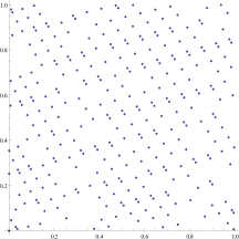
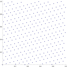
Figure 3: Comparison of rejected and original lattice points

3.1.6 When still not to use rejection with Monte Carlo

Another issue with the acceptance-rejection method is that it sometimes makes the dependence of the result of a Monte Carlo simulation on the model parameters less smooth. It is clear that the result of a true Monte Carlo simulation is by definition stochastic. If one looks for model parameters which minimize (a function of) the integral that is computed, then this has the paractical drawback that for example Newton’s method cannot be used. In practice it is therefore common to fix the random sequence for the Monte Carlo simulation, i.e., the random generator is started afresh for each set of parameters. In this sense the Monte Carlo method becomes closer to QMC, because the point set is now deterministic.

However, if acceptance-rejection is used for the generation of random variables, then the integral as a function of the model parameters can still be noisy. The following artificial example is taken from [6].

Example 3.8.

Let $\left(X_{i}^{\lambda}\right)_{i=1,\ldots,n}$ be a sequence of i.i.d. $\mathrm{Gamma}(\lambda,1)$ random variables and $S^{\lambda}=\sum_{i=1}^{n}X^{\lambda}_{i}$. Let further $f(s):=s-\bar{\lambda}\cdot n$.

We want to approximate

$$\alpha(\lambda)=\mathbb{E}\left[f(S^{\lambda})\right]$$

by the estimator

$$\hat{\alpha}_{N}(\lambda)=\frac{1}{N}\sum_{j=1}^{N}f(S^{\lambda}_{j})$$

for different values of $\lambda$, $\lambda\in(\bar{\lambda}-\epsilon,\bar{\lambda}+\epsilon)$. There are two scenarios:

1. We use a Monte Carlo method and acceptance-rejection with a suitable exponential distribution as dominating function. The pseudo number generator is restarted for every choice of $\lambda$, so that in fact we use the same sequence for every integral evaluation. The reason for this is that otherwise $\hat{\alpha}(\lambda)$ will be by itself random.

2. We use a low discrepancy quasi-Monte Carlo sequence (here: a Sobol sequence) together with the inverse transform method.

We draw those functions for $n=5,N=1024,\bar{\lambda}=2$ and $\epsilon=0.2$, where $\lambda$ changes in steps of $0.001$. In Figure 4 one can see quite some noise while in Figure 5 the graph is very smooth.

Smoothness is of importance if, for example, one wants to minimize $\alpha(\lambda)$. An application would be calibration of a financial model to market data.

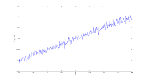
Figure 4: Acceptance-rejection method with a fixed Monte Carlo point set

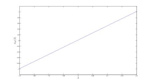
Figure 5: Inverse transform method with a quasi-Monte Carlo point set

3.2 Generation of Brownian paths

Many problems from finance, but also from physics, encompass phenomena which are modeled by a Brownian motion. In this section we give the basic definition and describe some methods for sampling from Brownian motion.

3.2.1 Brownian motion – definition and properties

Definition 3.9.

A standard Brownian motion $B$ in ${\mathbb{R}}^{d}$ is a stochastic process in continuous time, defined on some probability space $(\Omega,\Sigma,{\mathbb{P}})$, having the following properties:

1. $B_{0}=0$ almost surely;

2. $B$ has stationary increments, that is, for any $s,t\geq 0$ the random variables $B_{t+s}-B_{t}$ and $B_{s}$ have the same distribution;

3. $B$ has independent increments, that is, for any $n\in{\mathbb{N}}$ and any $t_{1},\ldots,t_{n}\in[0,\infty)$ with $t_{0}:=0<t_{1}<t_{2}<\ldots<t_{n}$, the random variables $B_{t_{1}}-B_{t_{0}},\ldots,B_{t_{n}}-B_{t_{n-1}}$ are independent;

4. $\sqrt{\frac{1}{t}}B_{t}$ is a standard normal ${\mathbb{R}}^{d}$-valued random variable for every $t\geq 0$;

5. $B$ has continuous paths, that is, for each $\omega\in\Omega$ the mapping $t\longmapsto B_{t}(\omega)$ is continuous.

For applications we usually only need to evaluate the Brownian path at finitely many nodes $t_{1},\ldots,t_{d}$. We therefore define a discrete Brownian path with discretization $0<t_{1}<\ldots<t_{d}$ as a Gaussian vector $(B_{t_{1}},\ldots,B_{t_{d}})$ with mean zero and covariance matrix

$$\big{(}\min(t_{j},t_{k})\big{)}_{j,k=1}^{d}=\left(\begin{array}[]{cccccccc}t_{1}&t_{1}&t_{1}&\ldots&t_{1}\\ t_{1}&t_{2}&t_{2}&\ldots&t_{2}\\ t_{1}&t_{2}&t_{3}&\ldots&t_{3}\\ \vdots&\vdots&\vdots&\ddots&\vdots\\ t_{1}&t_{2}&t_{3}&\ldots&t_{d}\end{array}\right)\,.$$

3.2.2 Classical constructions

There are three classical constructions of discrete Brownian paths:

• the forward method, also known as step-by-step method or piecewise method

• the Brownian bridge construction or Lévy-Ciesielski construction

• the principal component analysis construction (PCA construction)

The forward method is also the most straightforward one: given a standard normal vector $X=(X_{1},\ldots,X_{d})$ the discrete Brownian path is computed inductively by

$$B_{t_{1}}=\sqrt{t_{1}}X_{1}\,,\quad B_{t_{k+1}}=B_{t_{k}}+\sqrt{t_{k+1}-t_{k}}X_{k+1}\,.$$

Using that ${\mathbb{E}}(X_{j}X_{k})=\delta_{jk}$, it is easy to see that $(B_{t_{1}},\ldots,B_{t_{d}})$ has the required correlation matrix. Besides its simplicity, the main attractivity of the forward method lies in the fact that it is very efficient: given that the values $\sqrt{t_{k+1}-t_{k}}$ are pre-computed, generation of a path takes only generation of the normal vector plus $d$ multiplications and $d-1$ additions.

An alternative construction is the Brownian bridge construction, which allows the values $B_{t_{1}},\ldots,B_{t_{d}}$ to be computed in any given order. The main observation that makes this possible is the following lemma, the proof of which is left to the reader.

Lemma 3.10.

Let $B$ be a Brownian motion and let $r<s<t$.

Then the conditional distribution of $B_{s}$ given $B_{r},B_{t}$ is $N(\mu,\sigma^{2})$ with

$$\mu=\frac{t-s}{t-r}B_{s}+\frac{s-r}{t-r}B_{t}\text{ and }\sigma^{2}=\frac{(t-s)(s-r)}{t-r}\,.$$

Suppose the elements of $(B_{t_{1}},\ldots,B_{t_{d}})$ should be computed in the order $B_{t_{\pi(1)}},B_{t_{\pi(2)}},\ldots,B_{t_{\pi(d)}}$ for some permutation $\pi$ of $d$ elements. In computing $B_{t_{\pi(j)}}$ we need to take into account the previously computed elements, and at most two of those are of relevance, the one next to $\pi(j)$ on the left and the one next to $\pi(j)$ on the right: define for every $j\in\{1,\ldots,n\}$ two sets,

$$L(j) :=\{k:k<\pi(j)\;\text{and}\;\pi^{-1}(k)<j\}$$

$$R(j) :=\{k:k>\pi(j)\;\text{and}\;\pi^{-1}(k)<j\}\,.$$

Thus $L$ contains all the indices $k$ that are smaller than $\pi(j)$ and for which $B_{t_{k}}$ has already been constructed and $R$ contains all the indices $k$ that are greater than $\pi(j)$ and for which $B_{t_{k}}$ has already been constructed. Now define

$$l(j):=\left\{\begin{array}[]{cccc}0&\text{if}&L_{j}=\emptyset\\ \max L_{j}&\text{if}&L_{j}\neq\emptyset\end{array}\right.$$

$$r(j):=\left\{\begin{array}[]{cccc}\infty&\text{if}&R_{j}=\emptyset\\ \min R_{j}&\text{if}&R_{j}\neq\emptyset\end{array}\right.$$

and set $B_{t_{0}}=0$,

$$B_{t_{\pi(j)}}:=\left\{\begin{array}[]{ccccc}B_{t_{l(j)}}+\sqrt{t_{\pi(j)}-t_{l(j)}}X_{j}&\text{if}&r(j)=\infty\\[8.99994pt] \begin{array}[]{r}\frac{t_{r(j)}-t_{\pi(j)}}{t_{r(j)}-t_{l(j)}}B_{t_{l(j)}}+\frac{t_{\pi(j)}-t_{l(j)}}{t_{r(j)}-t_{l(j)}}B_{t_{r(j)}}\\ +\sqrt{\frac{(t_{\pi(j)}-t_{l(j)})(t_{r(j)}-t_{\pi(j)})}{t_{r(j)}-t_{l(j)}}}X_{j}\end{array}&\text{if}&r(j)<\infty\,,\end{array}\right.$$

where $X=(X_{1},\ldots,X_{d})$ is a standard normal random vector.

It is easy to check that the vector $(B_{t_{1}},\ldots,B_{t_{d}})$ constructed in that way has again covariance matrix $(\min(t_{j},t_{k}))_{j,k}$. The functions $l$ and $r$, as well as the factors of $B_{t_{l(j)}}$, $B_{t_{r(j)}}$, $Z_{j}$, do not depend on the random vector $X$ so they can be pre-computed. In some special cases the functions $l$ and $r$ can be computed explicitly, for example if the $\pi(t_{j})$ are the first $n$ elements of the van der Corput sequence or of the $\{k\alpha\}$-sequence with $\alpha=\frac{1+\sqrt{5}}{2}$, see [16]. Therefore the Brownian bridge construction is also very efficient: besides the generation of the vector $X$, computation of one sample uses at most $2d$ additions and $3d$ multiplications.

Moreover, we see that the forward construction is a special case of the Brownian bridge construction where $\pi$ is the identical permutation.

The PCA construction exploits the fact that the correlation matrix of $(B_{t_{1}},\ldots,B_{t_{d}})$ is positive definite and can therefore be written in the form $VDV^{-1}$ for a diagonal matrix $D$ with positive entries and an orthogonal matrix $V$. $D$ can be written as $D=D^{\frac{1}{2}}D^{\frac{1}{2}}$, where $D^{\frac{1}{2}}$ is the element-wise positive square root of $D$. Now the PCA construction from a standard normal random vector $X$ is given by

$$(B_{t_{1}},\ldots,B_{t_{d}})^{\top}=VD^{\frac{1}{2}}X\,.$$

The disadvantage of the PCA for high-dimensional problems is that the matrix-vector multiplication, having computational complexity $O(d^{2})$, becomes comparatively costly. Keiner and Waterhouse [14] describe an approximate PCA for which the cost of matrix-vector multiplication is $O(d\log d)$.

3.2.3 What is wrong about the forward construction?

We have provided three different constructions of Brownian paths with one standing apart in that it is clearly the most simple one. So why not use the forward construction for every application?

The answer is that theory predicts a big integration error for QMC if dimensions are big and the number of integration nodes is of realistic order, like a couple of millions only. But one may have the hope that if only a limited number input parameters have significant importance for the result, then QMC might behave very similar as in a low dimensional integration problem.

Figure 6 shows the influence of input parameters on the whole discrete path. We compare the forward construction on the left with the Brownian bridge construction on the right. In the two upper plots all but the first input variables are held fixed. We see that the influence of the first variable on the overall behavior of the path (in an informal sense) is bigger for the Brownian bridge construction.

In the two lower plots all but the 7th input variables are held fixed. We see that in the forward construction only values of the path after the seventh node are influenced, but the overall influence is only slightly smaller than that of the first variable. In contrast, the influence of the seventh variable in the Brownian bridge construction is restricted to the third quarter and is much smaller than that of the first variable.

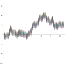
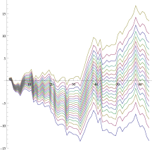
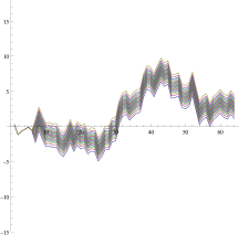
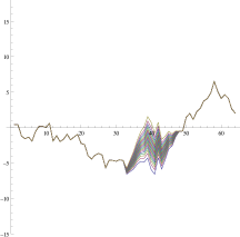
Figure 6: Paths of Brownian motion constructed with the forward construction (left) and the Brownian bridge construction (right). All but one parameters are fixed.

The above notion of “behaving like a low dimensional problem” is made precise in [3] with the notion of effective dimension. It must be added though, that despite of its popularity the concept of effective dimension alone does not fully explain the success of the alternative constructions. There is a great number of authors who investigated this problem and it is still largely unsolved at the present.

To answer the question posed in the header: there is nothing wrong with the forward construction, but for some classes of problems other constructions achieve lower errors, at least empirically. For other problems the forward construction may be just fine, as for example in the example due to [19], which will also be one of the examples in Section 3.5.

3.2.4 Evenly spaced discretization nodes

The case where the $t_{j}$ are evenly spaced is of special interest as will become apparent soon. In that case the covariance matrix equals

$$\Big{(}\frac{1}{d}\min(j,k)\Big{)}_{j,k=1}^{d}=\frac{1}{d}\left(\begin{array}[]{cccccccc}1&1&1&\ldots&1\\ 1&2&2&\ldots&2\\ 1&2&3&\ldots&3\\ \vdots&\vdots&\vdots&\ddots&\vdots\\ 1&2&3&\ldots&d\end{array}\right)\,.$$

We will denote this matrix by $\Sigma^{(d)}$ or, if there is no danger of confusion, simply by $\Sigma$.

Note that we can compute the Cholesky decomposition of $\Sigma$ rather easily: $\Sigma^{(d)}=SS^{\top}$, where

$$S=S^{(d)}:=\frac{1}{\sqrt{d}}\left(\begin{array}[]{cccccccc}1&0&0&\ldots&0\\ 1&1&0&\ldots&0\\ 1&1&1&\ldots&0\\ \vdots&\vdots&\vdots&\ddots&\vdots\\ 1&1&1&\ldots&1\end{array}\right)\,.$$

Note that if $y=(y_{1},\ldots,y_{d})$ is a vector in ${\mathbb{R}}^{d}$, then $Sy$ is the cumulative sum over $y$ divided by $\sqrt{d}$,

$$Sy=\frac{1}{\sqrt{d}}(y_{1},y_{1}+y_{2},\ldots,y_{1}+\ldots+y_{d})\,.$$

We have the following two easy lemmas:

Lemma 3.11.

Let $A$ be any $d\times d$ matrix with $AA^{\top}=\Sigma$ and let $X$ be a standard normal vector. Then $B=AX$ is a discrete Brownian path with discretization $\frac{1}{d},\frac{2}{d},\ldots,\frac{d-1}{d},1$.

Proof.

Since every linear combination of independent normal random variables is still normal, $AX$ is normal. We compute the covariance matrix:

$${\mathbb{E}}\left((AX)_{j}(AX)_{k}\right) ={\mathbb{E}}\left(\sum_{l=1}^{d}A_{jl}X_{l}\sum_{m=1}^{d}A_{km}X_{m}\right)$$

$$=\sum_{l=1}^{d}\sum_{m=1}^{d}A_{jl}A_{km}{\mathbb{E}}\left(X_{l}X_{m}\right)$$

$$=\sum_{l=1}^{d}A_{jl}A_{kl}=(AA^{\top})_{jk}=\Sigma_{jk}\,.$$

∎

Lemma 3.12.

Let $A$ be any $d\times d$ matrix with $AA^{\top}=\Sigma$. Then there is an orthogonal $d\times d$ matrix $V$ with $A=SV$. Conversely, $SV(SV)^{\top}=\Sigma$ for every orthogonal $d\times d$ matrix $V$.

Proof.

Suppose $AA^{\top}=\Sigma$, such that $AA^{\top}=SS^{\top}$. Note that $S$ is invertible and define $V=S^{-1}A$. Then

$$VV^{\top}=S^{-1}AA^{\top}(S^{-1})^{\top}=S^{-1}SS^{\top}(S^{-1})^{\top}=\mathrm{id}_{{\mathbb{R}}^{d}}\,,$$

showing that $V$ is orthogonal. The converse follows from the fact that for orthogonal $V$ we have $V^{\top}=V^{-1}$. ∎

For evenly spaced discretization nodes the orthogonal matrices corresponding to the classical matrices can often be given explicitly. The orthogonal transform corresponding to the forward method is the identical mapping on the ${\mathbb{R}}^{d}$. For $d=2^{k}$, the orthogonal transform corresponding to the Brownian bridge construction where $B$ is computed in the order $B_{1},B_{\frac{1}{2}},B_{\frac{1}{4}},B_{\frac{3}{4}},B_{\frac{1}{8}},B_{\frac{3}{8}},B_{\frac{5}{8}},\ldots$, is given by the inverse Haar transform, see [18]. For the PCA, the orthogonal transform has been given by Scheicher, and it has been shown that the computation complexity is $O(d\log(d))$, see [22]. The advantage of the representation of $A$ in Lemma 3.12 is that there are many orthogonal matrices that allow for fast matrix vector multiplication, that is, a path of length $d$ can be computed using $O(d\log(d))$ operations. Examples include the Walsh transform, discrete sine/cosine transform, Hilbert transform and others. See again [18].

Coming back to the general case of unevenly spaces discretization nodes we note the following: suppose you have nodes $0<t_{1}<\ldots<t_{d}$. We may compute an evenly spaced path $(B_{\frac{1}{d}},\ldots,B_{\frac{1}{d}})$ using our favorite orthogonal transform, then compute

$$\tilde{B}=\sqrt{d}\Big{(}\sqrt{t_{1}}B_{\frac{1}{d}},\sqrt{t_{2}-t_{1}}(B_{\frac{2}{d}}-B_{\frac{1}{d}}),\ldots,\sqrt{t_{d}-t_{d-1}}(B_{\frac{d}{d}}-B_{\frac{d-1}{d}})\Big{)}\,.$$

Then $\tilde{B}$ is a discrete Brownian path with discretization $0<t_{1}<\ldots<t_{d}$.

3.3 Generation of Lévy paths

Definition 3.13.

A Lévy process $L$ in ${\mathbb{R}}^{d}$ is a stochastic process in continuous time, defined on some probability space $(\Omega,{\cal F},{\mathbb{P}})$, having the following properties:

1. $L_{0}=0$ almost surely;

2. $L$ has stationary increments, that is, for any $s,t\geq 0$, the random variables $L_{s+t}-L_{t}$ and $L_{s}$ have the same distribution;

3. $L$ has independent increments, that is, for any $n\in{\mathbb{N}}$ and any $t_{1},\ldots,t_{n}\in[0,\infty)$ with $t_{0}:=0<t_{1}<t_{2}<\ldots<t_{n}$, the random variables $L_{t_{1}}-L_{t_{0}},\ldots,L_{t_{n}}-L_{t_{n-1}}$ are independent;

4. $L$ is continuous in probability, i.e., for all $t\geq 0$ and $c>0$,

   $$\lim_{h\rightarrow 0}{\mathbb{P}}(|L_{t+h}-L_{t}|>c)=0\,.$$

Without loss of generality one may also require (see [20, Chapter I.4, Theorem 30])

1. $L$ has càdlàg paths, that is, for each $\omega\in\Omega$ the mapping $t\longmapsto L_{t}(\omega)$ is right-continuous with limits from the left.

We will concentrate on discrete paths, and therefore properties 4. and 5. are of minor importance for our purpose. One property that follows from the above is that a Lévy process is already completely characterized by the distribution of $L_{1}$. Examples are provided by the Poisson process, where $L_{1}$ has Poisson distribution and by Brownian motion, where $L_{1}\sim N(0,1)$. The Lévy Kintchine formula (see [20, Chapter I.4, Theorem 43]) states that for any Lévy process there are numbers $b,\sigma\in{\mathbb{R}}$ and a measure $\nu$ on ${\mathbb{R}}\backslash\{0\}$ with $\int_{|x|<1}x^{2}\nu(dx)<\infty$ such that the characteristic function of $L_{t}$ is given by

$$\phi_{L_{t}}(u)={\mathbb{E}}\left(\exp(\mathrm{i}uL_{t})\right)=\exp(t\,\psi(u))$$

with

$$\psi(u)=\mathrm{i}bu-\frac{\sigma^{2}}{2}u^{2}+\int_{|x|\geq 1}(\exp(\mathrm{i}ux)-1)\nu(dx)+\int_{|x|<1}(\exp(\mathrm{i}ux)-1-\mathrm{i}ux)\nu(dx)\,.$$

Thus the distribution of $L_{t}$ (and therefore of an increment $L_{t+s}-L_{t}$) can be computed via Fourier inversion. For some distributions like the Normal, Poisson, and Gamma distribution, the density of the increment can be given explicitly.

It is actually straightforward to construct a discrete Lévy path on a given set of nodes $0<t_{1}<\ldots<t_{d}$ : let $F_{t}^{-1}$ denote the inverse of the distribution function of $L_{t}$. Let $U_{1},\ldots,U_{d}$ be independent $U(0,1)$ random variables. Define

$$L_{t_{1}} :=F_{t_{1}}^{-1}(U_{1})$$

$$L_{t_{k}} :=L_{t_{k-1}}+F_{t_{k}-t_{k-1}}^{-1}(U_{k})\,.$$

That is, the forward method works immediately. The other constructions have no direct generalizations to Lévy processes, except for special cases for which the conditional distribution of $L_{m}$ given $L_{l},L_{r}$ for $l<m<r$ can be computed. One such example is the Gamma process, the Lévy process for which $L_{t}$ has gamma distribution with parameters $(t\gamma,\lambda)$, $\gamma,\lambda\in(0,\infty)$, that is,

$${\mathbb{P}}(L_{t}\leq z)=\int_{0}^{z}\frac{x^{\gamma-1}}{\lambda^{\gamma}\Gamma(\gamma)}\exp(-x/\lambda)dx\,,$$

where it is shown in [2] that a Bridge construction is possible for this process and also for the variance-gamma process, which is a Lévy process of the form $t\mapsto W_{L_{t}}$, where $L$ is a gamma process and $W$ is Brownian motion.

However, there is a simple trick, first used in [17] for the Brownian bridge and later, but independently, in [11] for general orthogonal transforms, that recovers some of the qualitative features of those transforms: we may rewrite the forward construction of the discrete Lévy Path as

$$L_{t_{1}} :=F_{t_{1}}^{-1}(\Phi(Y_{1}))$$

$$L_{t_{k}} :=L_{t_{k-1}}+F_{t_{k}-t_{k-1}}^{-1}(\Phi(Y_{k}))\,,$$

where $Y_{1},\ldots,Y_{d}$ are independent standard normal variables and $\Phi$ is the standard normal CDF. The orthogonal transform is now employed simply in that the $Y_{1},\ldots,Y_{d}$ are generated from our input variables $X_{1},\ldots,X_{d}$ by multiplication with the orthogonal matrix, i.e. $Y=VX$.

Figure 7 illustrates the effect of this method on the construction of discrete normal inverse Gaussian (NIG) Lévy paths. The figure on the right shows the effect of the 7th input variable. In comparison to the corresponding Brownian motion example from figure 6 we see that the effect is less localized, but it still the seventh variable mostly influences the behavior of the path on the interval $[\frac{1}{2},\frac{3}{4}]$. Note that the plots are slightly misleading since they interpolate linearly between the discretization points and thus look like continuous functions. In reality, the paths of an NIG process are (with probability 1) discontinuous with infinitely many jumps in every non-empty open interval. It is important to keep this in mind if, for example, some characteristic of the first entry time of the path into some set is to be computed, as is the case, e.g., for barrier options.

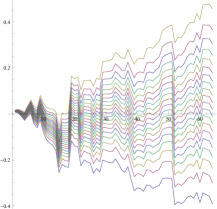
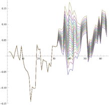
Figure 7: NIG process paths constructed with Brownian bridge orthogonal transform. Left figure: all but the first variables held fixed. Right figure: all but the 7th variable held fixed.

3.4 Multilevel (quasi-)Monte Carlo

Multilevel Monte Carlo is a technique for speeding up Monte Carlo simulation, especially for SDE models. It has gained a lot of recognition over the last couple of years, starting with the pioneering work by Giles [8] and Heinrich [10]. We give a short account of the method.

Suppose we want to approximate ${\mathbb{E}}(Y)$ for some random variable $Y$ which has finite expectation. Suppose further that we have a sequence of sufficiently regular functions $f^{\ell}:{\mathbb{R}}^{d_{\ell}}\rightarrow{\mathbb{R}}$ such that

$$\lim_{\ell\rightarrow\infty}{\mathbb{E}}(f^{\ell}(X^{\ell}))={\mathbb{E}}(Y)\,,$$ (11)

where for each $\ell\geq 0$, $X^{\ell}$ denotes a $d_{\ell}$-dimensional standard normal vector. In most cases the $f^{\ell}$ will be the discrete versions of a function defined on the Brownian paths with $d_{\ell}$ discretization nodes, and typically $d_{\ell}=2^{\ell}$. A standard examples is provided by the fixed strike Asian option, which has payoff

$$f(B):=\max\left(\frac{1}{T}\int_{0}^{T}S_{0}\exp\left(\sigma\sqrt{T}B_{t/T}+(r-\frac{\sigma^{2}}{2})t\right)dt\,,\,K\right)\,,$$

where $B$ is a standard Brownian motion, $S_{0}$ is the stock price at time $0$, $K$ is the strike of the option, $\sigma$ is the volatility and $r$ is the interest rate. $B$ will be approximated by a discrete path of the form $SV^{\ell}X^{\ell}$ where, for example, $V^{\ell}$ is the orthogonal transform corresponding to $d_{\ell}=2^{\ell}$-dimensional PCA.

Eqn. (11) states that there exists a sequence of algorithms which approximate ${\mathbb{E}}(Y)$ with increasing accuracy. For example, if $f^{\ell}(X^{\ell})$ has finite variance, we can approximate ${\mathbb{E}}(Y)$ by $\frac{1}{N}\sum_{k=0}^{N-1}f^{\ell}(X^{\ell}_{k})$ using sufficiently large $\ell$ and $N$, where $(X^{\ell}_{k})_{k\geq 0}$ is a sequence of independent standard normal vectors.

Usually, evaluation of $f^{\ell}(X^{\ell}_{k})$ becomes more costly with increasing $\ell$. Multilevel methods sometimes help us to save significant proportions of computing time by computing more samples for the coarser approximations, which need less computing time but have higher variance.

We have, for large $L$,

$${\mathbb{E}}(Y) \approx{\mathbb{E}}\left(f^{L}(X^{L})\right)$$ (12)

$$={\mathbb{E}}\left(f^{0}(X^{0})\right)+\sum_{\ell=1}^{L}{\mathbb{E}}\left(f^{\ell}(X^{\ell})\right)-{\mathbb{E}}\left(f^{\ell-1}(X^{\ell-1})\right)$$

$$={\mathbb{E}}\left(f^{0}(X^{0})\right)+\sum_{\ell=1}^{L}{\mathbb{E}}\left(f^{\ell}(X^{\ell})\right)-{\mathbb{E}}\left(f_{c}^{\ell-1}(X^{\ell})\right)$$

$$={\mathbb{E}}\left(f^{0}(X^{0})\right)+\sum_{\ell=1}^{L}{\mathbb{E}}\left(f^{\ell}(X^{\ell})-f_{c}^{\ell-1}(X^{\ell})\right)\,,$$

where $(f_{c}^{\ell})_{\ell\geq 0}$ is an arbitrary sequence of functions $f_{c}^{\ell}:{\mathbb{R}}^{d_{\ell+1}}\rightarrow{\mathbb{R}}$ with ${\mathbb{E}}(f_{c}^{\ell-1}(X^{\ell}))={\mathbb{E}}(f^{\ell}(X^{\ell}))$. The “c” in $f_{c}^{\ell}$ stands for “coarse level”.

The most basic example for $f_{c}^{\ell}$ is given for $d_{\ell}=m^{\ell}$ by $f_{c}^{\ell}=f^{\ell}\circ C_{m,\ell}$, where $C_{m,\ell}$ is the linear map defined by the matrix

$$(C_{m,\ell})_{i,j}:=\left\{\begin{array}[]{cl}\frac{1}{\sqrt{m}}&\quad\mbox{ if }~{}(i-1)m+1\leq j\leq i\,m\,,\;1\leq i\leq m^{\ell}\\ 0&\quad\mbox{ else }\end{array}\right.\,.$$

For example,

$$C_{2,\ell}:=\left(\begin{array}[]{cccccccc}\frac{1}{\sqrt{2}}&\frac{1}{\sqrt{2}}&0&0&0&\dots&0&0\\ 0&0&\frac{1}{\sqrt{2}}&\frac{1}{\sqrt{2}}&0&\dots&0&0\\ \vdots&\vdots&\vdots&\vdots&\vdots&&\vdots&\vdots\\ 0&0&0&0&0&\dots&\frac{1}{\sqrt{2}}&\frac{1}{\sqrt{2}}\end{array}\right)\,.$$

In general, $f_{c}^{\ell}$ is chosen in a way to get small variances for the $f^{\ell}(X^{\ell})-f_{c}^{\ell-1}(X^{\ell})$.

Equation (12) becomes useful if, as is often the case in practice, the expectation ${\mathbb{E}}\left(f^{\ell}(X^{\ell})-f^{\ell-1}(C_{m,\ell}X^{\ell})\right)$ can be approximated to the required level of accuracy using less function evaluations $N_{\ell}$ for bigger $\ell$ while the costs $c_{\ell}$ per function evaluation increases. Suppose the error of approximation of ${\mathbb{E}}\left(f^{\ell}(X^{\ell})-f_{c}^{\ell-1}(X^{\ell})\right)$ using $N_{\ell}$ points is $e_{\ell}(N_{\ell})$. We choose $N_{0},\ldots,N_{L}$ so that

$$e_{0}(N_{0})+\ldots+e_{L}(N_{L})\leq\varepsilon$$

while minimizing the total cost

$$c=c_{0}N_{0}+\ldots+c_{L}N_{L}\,.$$

In that way the total computation cost is typically much lower than it would be if ${\mathbb{E}}(f^{L}(X^{L}))$ would be computed directly.

One typical situation is the numerical solution of a stochastic differential equation using time discretization with $d_{\ell}$ time steps and $f^{\ell}$ is some function on the set of solution paths. See [8] for how to exploit this representation for Monte Carlo simulation. See also [7] for the combination of the multilevel technique with QMC.

3.5 Examples

Consider the problem of valuating an Asian option in the Heston model. We solve the SDE using the simple Euler-Maruyama method eqn. (5). The model parameters are $s_{0}=100$, $v_{0}=0.3$, $r=0.03$, $\rho=0.2$, $\kappa=2$, $\theta=0.3$, $\xi=0.5$, the option parameters are $K=100$, $T=1$. The SDE is solved using a two-dimensional Brownian motion with 32 equally spaced time steps. For that we need 64 independent standard normal variables per QMC evaluation. Since the problem is relatively high-dimensional we want to apply an orthogonal transform to the input variables. It is near at hand to apply one transform for each of the two Brownian paths, but at least for this example it seems to be better to use one 64-dimensional transform.

We use the classical Sobol sequence for integration. We add a 64-dimensional random shift to the sequence and plot the $\log_{2}$ of the standard deviation over $64$ integral evaluations each using $2^{m}$ points of the sequence, $m=2,\ldots,10$.

The left hand graph Figure 8 shows the $\log_{2}$ of the standard deviation along $m$ for 4 different transforms: the identity, “Forward”, the orthogonal transform corresponding to the Brownian bridge (i.e., the inverse Haar transform), “BB”, the one corresponding to PCA and the Brownian bridge applied separately to the inputs of the two Brownian paths, “BB2”. On the $x$ axis we plot the $\log_{2}$ of the number of integration points, i.e., $m$, while along the $y$ axis we plot the $\log_{2}$ of the standard deviation of the result over $64$ runs.

We can see that, as in many practical examples, the PCA performs best. Maybe surprisingly the idea of using two independent Brownian bridge constructions performs worse than the two combined transforms, but still much better than the identical transform.

We complement this graph be the corresponding one for the example from [19]. The payoff of this “ratchet” option is

$$f(S_{\frac{T}{d}},S_{\frac{2T}{d}},\ldots,S_{T})=\frac{1}{d}\sum_{j=1}^{d}1_{[0,\infty)}\left(S_{\frac{jT}{d}}-S_{\frac{(j-1)T}{d}}\right)S_{\frac{jT}{d}}\,.$$

The errors are plotted on the right hand side of 8. We can see that the orthogonal transforms that were so successful in the case of an Asian option now perform worse then the identity.

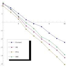
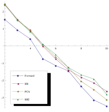
Figure 8: Left: Convergence of the price of an Asian option under different transforms. Right: same graph for the ratchet option.

Thus it has to be kept in mind that the choice of the orthogonal transform has to be in line with the payoff function. How this should be done exactly, and for which types of payoffs it accelerates convergence, is still subject to research. See for example [12, 13], where it is tried to choose the orthogonal transform in a way that puts as much variance as possible into the dependence of the first input variable. To this end the payoff is approximated by a linear function $g$ (“regression”) and an orthogonal (Householder-)transform $V$ is computed such that $g\circ V$ only depends on $X_{1}$. This $V$ is taken as the orthogonal transform for the original problem.

We conclude with an example in which multilevel Monte Carlo is combined with orthogonal transforms and QMC. We compare the multilevel QMC method together with the regression algorithm from [12] with multilevel Monte Carlo and multilevel quasi-Monte Carlo (forward and PCA sampling) numerically. For that we choose the parameters in a Black-Scholes model as $r=0.04$, $\sigma=0.3$, $S_{0}=100$, and we aim to value an Asian call option with parameters $K=100$ and $T=1$. At the finest level we choose $2^{10}$ discretization points and at each coarser level the number of points is divided in by 2, i.e. $L=10$ and $m=2$. The number of sample points are doubled at each level starting with $N_{L}$ sample points at the finest level $L$. For the QMC approaches we take a Sobol sequence with a random shift. In Table 1 we compare for different values $N_{L}$ both the average and the standard deviation of the price of the Asian call option based on $1000$ independent runs. Moreover, the average computing time for one run is given in brackets. As we can see, the regression algorithm yields the lowest standard deviation, but the computing time of the regression algorithm is slightly higher than that for the forward method. The regression algorithm outperforms the PCA construction measured both by standard deviation and computing time.

	multilevel		multilevel QMC
	Monte Carlo		forward		PCA		regression
$N_{L}$	average	stddev	average	stddev	average	stddev	average	stddev
2	7.717	$0.41\times 10^{0}$	7.735	$0.19\times 10^{-1}$	7.736	$0.16\times 10^{-1}$	7.739	$0.10\times 10^{-1}$
	(0.0057 s)		(0.0057 s)		(0.0088 s)		(0.0069 s)
4	7.738	$0.19\times 10^{0}$	7.734	$0.71\times 10^{-2}$	7.736	$0.44\times 10^{-2}$	7.738	$0.29\times 10^{-2}$
	(0.0074 s)		(0.0074 s)		(0.0118 s)		(0.0091 s)
8	7.748	$0.54\times 10^{-1}$	7.737	$0.30\times 10^{-2}$	7.737	$0.14\times 10^{-2}$	7.736	$0.10\times 10^{-2}$
	(0.0101 s)		(0.0100 s)		(0.0165 s)		(0.0124 s)
16	7.746	$0.40\times 10^{-1}$	7.736	$0.11\times 10^{-2}$	7.737	$0.69\times 10^{-3}$	7.736	$0.30\times 10^{-3}$
	(0.0157 s)		(0.0157 s)		(0.0279 s)		(0.0194 s)
32	7.728	$0.31\times 10^{-1}$	7.736	$0.49\times 10^{-3}$	7.737	$0.21\times 10^{-3}$	7.736	$0.10\times 10^{-3}$
	(0.0266 s)		(0.0265 s)		(0.0585 s)		(0.0326 s)
64	7.739	$0.81\times 10^{-2}$	7.736	$0.20\times 10^{-3}$	7.737	$0.69\times 10^{-4}$	7.737	$0.32\times 10^{-4}$
	(0.0486 s)		(0.0484 s)		(0.1202 s)		(0.0583 s)

Table 1: Multilevel (Q)MC using $2^{10}$ time steps $(L=10)$. The average and the standard deviation of the option price are based on $1000$ runs. The average computing time is given in brackets.

References

- [1] L. Andersen. Simple and efficient simulation of the heston stochastic volatility model. Journal of Computational Finance, 11(3), 2008.
- [2] A. N. Avramidis and P. L’Ecuyer. Efficient Monte Carlo and quasi-Monte Carlo option pricing under the variance gamma model. Manage. Sci., 52:1930–1944, 2006.
- [3] R. E. Caflisch, W. Morokoff, and A. Owen. Valuation of mortgage-backed securities using Brownian bridges to reduce effective dimension. The Journal of Computational Finance, 1(1):27–46, 1997.
- [4] R. Cont and P. Tankov. Financial Modelling with Jump Processes. Chapman & Hall/Crc Financial Mathematics Series. Chapman & Hall/CRC, 2012.
- [5] F. Delbaen and W. Schachermayer. The Mathematics of Arbitrage. Springer, 2006.
- [6] A. Eichler, G. Leobacher, and H. Zellinger. Calibration of financial models using quasi-Monte Carlo. Monte-Carlo Methods Appl., 17(2):99–131, 2011.
- [7] M. Giles and B. Waterhouse. Multilevel quasi-Monte Carlo path simulation. Radon Series Comp. Appl. Math., 8:1–18, 2009.
- [8] M. B. Giles. Multilevel Monte Carlo path simulation. Oper. Res., 56(3):607–617, 2008.
- [9] P. Glasserman. Monte Carlo methods in financial engineering. Springer, 2004.
- [10] S. Heinrich. Multilevel monte carlo methods. In S. Margenov, J. Waśniewski, and P. Yalamov, editors, Large-Scale Scientific Computing, volume 2179 of Lecture Notes in Computer Science, pages 58–67. Springer Berlin Heidelberg, 2001.
- [11] J. Imai and K. S. Tan. An accelerating quasi-Monte Carlo method for option pricing under the generalized hyperbolic Lévy process. SIAM J. Sci. Comput., 31(3):2282–2302, 2009.
- [12] C. Irrgeher and G. Leobacher. Fast orthogonal transforms for pricing derivatives with quasi-Monte Carlo. In C. Laroque, J. Himmelspach, R. Pasupathy, O. Rose, and A. M. Uhrmacher, editors, Proceedings of the 2012 Winter Simulation Conference, 2012.
- [13] C. Irrgeher and G. Leobacher. Fast orthogonal transforms for multilevel quasi-Monte Carlo simulation in computational finance. In Vanmaele, W. et al., editor, Proceedings of Actuarial and Financial Mathematics Conference 2013: Interplay between Finance and Insurance, 2013.
- [14] J. Keiner and B. J. Waterhouse. Fast principal components analysis method for finance problems with unequal time steps. L’Ecuyer, Pierre (ed.) et al., Monte Carlo and quasi-Monte Carlo methods 2008. Proceedings of the 8th international conference Monte Carlo and quasi-Monte Carlo methods in scientific computing, Montréal, Canada, July 6–11, 2008. Berlin: Springer. 455-465 (2009)., 2009.
- [15] P. E. Kloeden and E. Platen. Numerical Solution of Stochastic Differential Equations. Springer, Berlin, 1992.
- [16] G. Larcher, G. Leobacher, and K. Scheicher. On the tractability of the Brownian bridge algorithm. J. Complexity, 19:511–528, 2003.
- [17] G. Leobacher. Stratified sampling and quasi-Monte Carlo simulation of Lévy processes. Monte-Carlo methods and applications, 12(3-4):231–238, 2006.
- [18] G. Leobacher. Fast orthogonal transforms and generation of Brownian paths. J. Complexity, 28(2):278–302, 2012.
- [19] A. Papageorgiou. The Brownian bridge does not offer a consistent advantage in quasi-Monte Carlo integration. J. Complexity, 18(1):171–186, 2002.
- [20] P. E. Protter. Stochastic integration and differential equations. 2nd ed. Springer, 2004.
- [21] L. C. G. Rogers and Z. Shi. The Value of an Asian Option. Journal of Applied Probability, 32(4):1077–1088, 1995.
- [22] K. Scheicher. Complexity and effective dimension of discrete Lévy areas. J. Complexity, 23(2):152–168, 2007.