Kernel Method for Detecting Higher Order Interactions in multi-view Data: An Application to Imaging, Genetics, and Epigenetics

Abstract

Technological advances are enabling us to collect multiple types of data at an increasing depth and resolution while decreasing the labor needed to compile and analyze it. A central goal of multimodal data integration is to understand the interaction effects of different features. Understanding the complex interaction among multimodal datasets, however, is challenging. In this study, we tested the interaction effect of multimodal datasets using a novel method called the kernel method for detecting higher order interactions among biologically relevant mulit-view data. Using a semiparametric method on a reproducing kernel Hilbert space (RKHS), we used a standard mixed-effects linear model and derived a score-based variance component statistic that tests for higher order interactions between multi-view data. The proposed method offers an intangible framework for the identification of higher order interaction effects (e.g., three way interaction) between genetics, brain imaging, and epigenetic data. Extensive numerical simulation studies were first conducted to evaluate the performance of this method. Finally, this method was evaluated using data from the Mind Clinical Imaging Consortium (MCIC) including single nucleotide polymorphism (SNP) data, functional magnetic resonance imaging (fMRI) scans, and deoxyribonucleic acid (DNA) methylation data, respectfully, in schizophrenia patients and healthy controls. We treated each gene-derived SNPs, region of interest (ROI) and gene-derived DNA methylation as a single testing unit, which are combined into triplets for evaluation. In addition, cardiovascular disease risk factors such as age, gender, and body mass index were assessed as covariates on hippocampal volume and compared between triplets. Our method identified $13$-triplets ($p$-values $\leq 0.001$) that included $6$ gene-derived SNPs, $10$ ROIs, and $6$ gene-derived DNA methylations that correlated with changes in hippocampal volume, suggesting that these triplets may be important in explaining schizophrenia-related neurodegeneration. With strong evidence ($p$-values $\leq 0.000001$), the triplet (MAGI2, CRBLCrus1.L, FBXO28) has the potential to distinguish schizophrenia patients from the healthy control variations. This novel method may shed light on other disease processes in the same manner, which may benefit from this type of multimodal analysis.

keywords: Multimodal data, Higher order interaction, Kernel methods, Imaging genetics, Imaging epigenetics, and Schizophrenia.

1 Introduction

The advancements in data science technology over the last decade has rapidly evolved to collect multi-view data, which has emerged to provide a comprehensive way to explore statistical structures and information embedded in the relationship between datasets. The integration of imaging and genetic information into a format capable of predicting disease phenotypes, however, continues to be challenging problem.

One of the goals of imaging genetics is the modeling and understanding of how genetic variations influence the structure and function of brain disease. This goal can be achieved by collating multimodal data including functional magnetic resonance imaging (fMRI), structural MRI (sMRI), and positron emission tomography (PET) scans with single nucleotide polymorphisms (SNPs), deoxyribonucleic acid (DNA) methylations, gene expression (GE), transcriptomics, epigenomics, and proteomics factors. Numerous studies have suggested that these different factors do not act in isolation, but rather they interact at multiple levels and depend on one another in an intertwined manner Calhoun  Sui (2016); Pearlson . (2015). Extracting the interaction effects from within and among data sets, however, remains a challenge for multi-view data analysis J. Li . (2015); Chekouo . (2016); Zheng . (2015); Zhao . (2016); M. Liu . (2016). Figure 1 illustrates how the interaction effects of different data sets can be used to model and predict human illness.

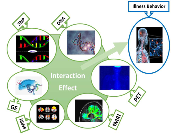
Figure 1: An illustration of the different imaging genetics and epigenetics data along with their interaction effect on human behavior. Note, SNP: single nucleotide polymorphism, DNA: deoxyribonucleic acid methylations, PET: positron emission tomography (PET), fMRI: functional magnetic resonance imaging (fMRI), sMRI: structural MRI, GE: gene expression.

To date, both genetic techniques and brain imaging have played a substantial role in detecting disease phenotypes. For example, by correlating imaging and genetic data, it has been shown that certain genes affect specific brain functions, connectivity, and serve as risk predictors for certain diseases. Jahanshad . (2012); Lin . (2014); Bis . (2012); Jahanshad  X. Hua (2013). Additionally, Bis . (2012) have identified genetic variants affecting the volume of the hippocampus, which could be used as predictors of cognitive decline and dementia Jahanshad  X. Hua (2013). As shown in Wen . (2017), accurate identification of Tourette’s syndrome in children has notably improved using multi-view features as compared to relying solely on one view. Accumulating evidence also shows that the inherent genetic variations for complex traits can sometimes be explained by the joint analysis of multiple genetic features with environmental factors.

Schizophrenia (SZ) is a complex brain disorder that affects how a person thinks, feels and acts, which is thought to be caused through an interplay of genetic effects, brain region, and DNA methylation abnormalities Richfield . (2017). Studies using neurological tests and brain imaging technologies (fMRI and PET) have been used to examine functional differences in brain activity that seem to arise within the frontal lobes, hippocampus and temporal lobes Van  Kapur (2009); Kircher  Renate (2005). Many researchers have shown that genetic alterations at the mRNA and SNP level, however, also play a significant role in SZ Chang . (2013); Lencz . (2007). Thus, only focusing on brain imaging data is not sufficient in the identification of the related risk factors for SZ Potkin . (2015). To address this, Chekouo . (2016) have developed the ROI-SNP network for the selection of discriminatory markers using brain imaging and genetics information.

A number of studies suggest that epigenetics also has a role in SZ disease susceptibility. Genome-wide DNA methylation analysis of human brain tissue from SZ patients shows a heritable epigenetic modification, which can regulate gene expression. The cell specific differences in chromatin structure that influence cell development, including DNA methylation, have emerged as a potential explanation for the non-Mendelian inheritance of SZ Wockner . (2014). There is also evidence on epigenetic alterations in the blood and central nervous system of patients with SZ, and it has been shown that methylation status in brain tissue from SZ patients varies significantly from controls Aberg . (2014); Montano . (2016). In this paper, we consider the interaction effects among the genetics, brain imaging, and epigenetics data on hippocampal volume measurements between SZ patients and healthy controls using a novel kernel method for detecting these higher order interactions.

Many advancements in multimodal fusion methods have utilized such approaches as co-training, multi-view learning, subspace learning, multi-view embedding, and kernel multiple learning, to analyze multi-view data of biological relevance Xu . (2013). However, due to the large number of genes, SNPs, DNA methylations and different types of imaging, positive definite kernel based methods have become a popular and effective tool for conducting genome-wide association studies (GWASs) and imaging genetics, especially for identifying genes associated with diseases S. Li  Cui (2012); Ge . (2015); Alam, Calhoun  Wang (2016); Alam, Komori . (2016). Kernel methods are emerging as innovative techniques that map data from high dimension input spaces to a kernel feature space using a nonlinear function. The main advantage of these methods is to combine statistics and geometry in an effective way Hofmann . (2008). Kernel methods offer useful algorithms to learn how a large number of genetic variants are associated with complex phenotypes, to help explore the relationship between the genetic markers and the outcome of interest Camps-Valls . (2007); S. Yu  Moreau (2011); Alam (2014); Alam  Fukumizu (2015); Schölkopf . (1998); Kung (2014).

In genetics, the detection of gene-gene interactions or co-associations in most methods are divided into two types: SNP based and gene-based methods in GWASs. In the last decade, a number of statistical methods have been used to detect gene-gene interactions (GGIs). Logistic regression, multifactor dimensionality reduction, linkage disequilibrium and entropy based statistics are examples of such methods Hieke . (2014); Wan . (2010). While most of these methods are based on the unit association of the SNPs, testing the associations between the phenotype and SNPs has limitations and is not sufficient for interpretation of GGIs Yuan . (2012). In GWASs, gene-based methods are always more effective than the ones based only on a SNP, and powerful tools for multivariate gene-based genome-wide associations have been proposed Sluis . (2015).

In recent years, linear, kernel, and robust canonical correlation based U statistic have been utilized to identify gene-gene co-associations Peng . (2010); Alam, Komori . (2016). S. Li  Cui (2012) have proposed a model-based kernel machine method for GGIs. In addition, Ge . (2015) have also proposed a kernel machine method for detecting effects of interactions between multi-variable sets. This is an extended model of S. Li  Cui (2012) to jointly model the genetics and non-genetic features, and their interactions. While these methods could ultimately shed light on novel features of the etiology of complex diseases, they cannot be reliable used in multi-view data sets. Thus, there exists a need to extend kernel machine based methods.

The contribution of this paper, therefore, is threefold. By examining the three-way interaction effects between triplet data sets combining genetics, imaging, and epigenetics, we hope to shed light on the phenotype features associated with disease mechanisms. This is done iteratively. First, we propose a novel semiparametric method on a reproducing kernel Hilbert space (RKHS) to study the interaction effects among the multiple-view datasets. We name a kernel method for detecting higher order interactions (KMDHOI) and include the pairwise and higher order Hadamard product of the features from different views. Second, we formulate the problem as a standard mixed-effect linear model to derive a score-based variance component test for the higher order interactions. The proposed method offers a flexible framework to account for the main (single), pairwise, triplet, other higher order effects and test for the overall higher order effects. Finally, we validate the proposed method on both simulation and the Mind Clinical Imaging Consortium (MCIC) data J. Chen . (2012); Gollub . (2013).

The remainder of this paper is organized as follows. In Section 2, we propose a standard mixed-effects linear model to derive score-based variance component test for higher order interaction. In Section 3, we propose statistical testing for higher order interaction effects. The relevant methods are discussed in Section 4. In Section 5, we describe the experiments conducted on both synthesized and the imaging genetics data sets. We conclude the paper with a discussion of major findings and future research in Section 6. Details of the theoretical analysis for the proposed method, Satterthwaite approximation to the score test, and supplementary tables and figures on application to imaging genetics and epigenetics can be found in the appendix.

2 Method

In kernel methods, the nonlinear feature map is given by a positive definite kernel, which provides nonlinear methods for data analysis. It is known Aronszajn (1950) that a positive definite kernel $k$ is associated with a Hilbert space $\mathcal{H}$, called reproducing kernel Hilbert space (RKHS), consisting of functions on $\mathcal{X}$ so that the function value is reproduced by the kernel; namely, for any function $f\in\mathcal{H}$ and a point $X\in\mathcal{X}$, the function value $f(X)$ is $f(X)=\langle f(\cdot),k(\cdot,X)\rangle_{\mathcal{H}},$ where $\langle,\rangle_{\mathcal{H}}$ in the inner product of $\mathcal{H}$ is called the reproducing property. Replacing $f$ with $k(\cdot,\tilde{X})$ yields $k(X,\tilde{X})=\langle k(\cdot,X),k(\cdot,\tilde{X})\rangle_{\mathcal{H}}$ for any $X,\tilde{X}\in\mathcal{X}$. A symmetric kernel $k(\cdot,\cdot)$ defined on a space $\mathcal{X}$ is called positive definite, if for an arbitrary number of points $X_{1},\ldots,X_{n}\in\mathcal{X}$ the Gram matrix $(k(X_{i},Y_{j}))_{ij}$ is positive semi-definite. To transform data for extracting nonlinear features, the mapping $\mathbf{\Phi}:\mathcal{X}\to\mathcal{H}$ is defined as $\mathbf{\Phi}(X)=k(\cdot,X),$ which is a function of the first argument. This map is called the feature map, and the vector $\mathbf{\Phi}(X)$ in $\mathcal{H}$ is called the feature vector. The inner product of two feature vectors is then $\langle\mathbf{\Phi}(X),\mathbf{\Phi}(\tilde{X})\rangle_{\mathcal{H}}=k(X,\tilde{X}).$ This is known as the kernel trick. By this trick the kernel can evaluate the inner product of any two feature vectors efficiently without knowing an explicit form of $\mathbf{\Phi}(\cdot)$.

2.1 Model setting

Assuming that we have $n$ independent identical distributed (IID) subjects $y_{i}$ $(i=1,2,\cdots,n)$ with $(q-1)$ covariates $X_{i}=[X_{i1},X_{i2}\cdots X_{i(q-1)}]^{T}$ and m-view datasets, $\mathbf{M}_{i}^{(1)},\cdots,\mathbf{M}_{i}^{(m)}$. In the following semiparametric model, we associate the output $y_{i}$ with covariates including intercept and $m$-view datasets:

$$y_{i}=X_{i}^{T}\mathbf{\boldsymbol{\beta}}+f(\mathbf{M}_{i}^{(1)},\cdots,\mathbf{M}_{i}^{(m)})+\epsilon_{i},$$ (1)

where $X_{i}$ is a $q\times 1$ vector of covariates including intercept for the $i-$th subject, $\boldsymbol{\beta}$ is a $q\times 1$ vector of fixed effects, $f$ is an unknown function on the product domain, $\mathcal{M}=\mathcal{M}^{(1)}\otimes\mathcal{M}^{(2)}\otimes,\cdots,\otimes\mathcal{M}^{(m)}$ with $\mathbf{M}_{i}^{(\ell)}\in\mathcal{M}_{\ell},\ell=1,2,\cdots m$ and the error $\epsilon_{i}$’s are IID as normal with mean zero and variance $\sigma^{2}$, $\epsilon_{i}\sim\rm{NIID}(0,\sigma^{2})$. According to the ANOVA decomposition, the function, $f$ can be extended as:

$$f(\mathbf{M}^{(1)}_{i},\cdots,\mathbf{M}^{(m)}_{i})=\sum_{\ell=1}^{m}h_{\mathbf{M}^{(\ell)}}(\mathbf{M}_{i}^{(\ell)})+\sum_{\ell_{1}>\ell_{2}}h_{\mathbf{M}^{(\ell_{1})},\mathbf{M}^{(\ell_{2})}}(\mathbf{M}^{(\ell_{1})}_{i},\mathbf{M}^{(\ell_{2})}_{i})+\\ \sum_{\ell_{1}>\ell_{2}>\ell_{3}}h_{\mathbf{M}^{(\ell_{1})}\times\mathbf{M}^{(\ell_{2})}\times\mathbf{M}^{(\ell_{3})}}(\mathbf{M}^{(\ell_{1})}_{i},\mathbf{M}^{(\ell_{2})}_{i},\mathbf{M}^{(\ell_{3})}_{i})+\cdots+h_{\mathbf{M}^{(1)}\times\mathbf{M}^{(2)}\times\mathbf{M}^{(3)}\times\cdots,\times\mathbf{M}^{(m)}}(\mathbf{M}^{(1)}_{i},\mathbf{M}^{(2)}_{i},\cdots,\mathbf{M}^{(m)}_{i}),$$ (2)

where $h_{\mathbf{M}^{(\ell)}}(\mathbf{M_{i}}^{(\ell)})$’s ($\ell:1,2,\cdots m$) are the main effects for the respective dataset, $h_{{\mathbf{M}^{(\ell_{1})}},{\mathbf{M}^{(\ell_{2})}}}(\mathbf{M}_{i}^{(\ell_{1})},\mathbf{M}_{i}^{(\ell_{2})})$ are pairwise interactions effects, $h_{{\mathbf{M}^{(\ell_{1})}}\times{\mathbf{M}^{(\ell_{2})}},{\mathbf{M}^{(\ell_{3})}}}(\mathbf{M}_{i}^{(\ell_{1})},\mathbf{M}_{i}^{(\ell_{2})},\mathbf{M}_{i}^{(\ell_{3})})$ are the interactions effects of the three dataset and so on. The functional space, RKHS, is decomposes as:

$$\mathcal{H}=\mathcal{H}_{\mathbf{M}^{(1)}}\oplus\mathcal{H}_{\mathbf{M}^{(2)}}\oplus\cdots\oplus\mathcal{H}_{\mathbf{M}^{(m)}}\oplus\mathcal{H}_{\mathbf{M}^{(1)}\times\mathbf{M}^{(2)}}\oplus\mathcal{H}_{\mathbf{M}^{(1)}\times\mathbf{M}^{(3)}}\oplus\cdots\oplus\mathcal{H}_{\mathbf{M}^{(1)}\times\mathbf{M}^{(m)}}\oplus\mathcal{H}_{\mathbf{M}^{(2)}\times\mathbf{M}^{(3)}}\\ \oplus\cdots\oplus\mathcal{H}_{\mathbf{M}^{(1)}\times\mathbf{M}^{(2)}\times\mathbf{M}^{(3)}}\oplus\cdots\oplus\mathcal{H}_{\mathbf{M}^{(1)}\times\mathbf{M}^{(2)}\times\cdots\times\mathbf{M}^{(m)}},$$ (3)

equipped with an inner product, $\langle\cdot,\cdot\rangle$ and a norm $\|\cdot\|_{\mathcal{H}}.$ If $m=1$, Eq. (1) becomes simple semiparametric regression model as shown in D. Liu . (2007). S. Li  Cui (2012) and Ge . (2015) have proposed similar models (special case of Eq. (1), $m=2$) for detecting interaction effects among multidimensional variable sets.

Specifically, in our case we have three data sets. To do this, we assume that we have $n$ IID subjects under investigation; $y_{i}\,(i=1,2,\cdots n)$ is a quantitative phenotype for the $i$-th subject (say, hippocampal volume derived from structural MRI scan). We associate the clinical covariates (e.g., age, weight, height) with three views: genetics, imaging, and epigentics (gene-derived SNP, ROIs, and gene-derived DNA methylation). Let $\mathbf{X}_{i}$ denote the $(q-1)$ covariates, where $X_{ij},j=1,2,\cdots(q-1)$ is a measure of the $i$-th subject. Let $M_{i}^{(1)}=[M_{i1}^{(1)},M_{i2}^{(1)},\cdots,M_{is}^{(1)}]$, $M_{i}^{(2)}=[M_{i1}^{(2)},M_{i2}^{(2)},\cdots,M_{is}^{(2)}]$ and $M_{i}^{(3)}=[M_{i1}^{(3)},M_{i2}^{(3)},\cdots,M_{is}^{(3)}]$ be a genes-derived SNP with $s$ SNP markers, a ROI with $r$ voxels of the fMRI scan, and a gene-derived DNA methylation with $d$ methylation profiles of the $i$-th subject, respectively. Under this setting, Eq. (1), Eq. (2) and Eq. (3) become:

$$y_{i}=X_{i}^{T}\mathbf{\boldsymbol{\beta}}+f(\mathbf{M}_{i}^{(1)},\mathbf{M}_{i}^{(2)},\mathbf{M}_{i}^{(3)})+\epsilon_{i},$$ (4)

$$f(\mathbf{M}^{(1)}_{i},\mathbf{M}^{(2)}_{i},\mathbf{M}^{(3)}_{i})=h_{\mathbf{M}^{(1)}}(\mathbf{M}_{i}^{(1)})+h_{\mathbf{M}^{(2)}}(\mathbf{M}_{i}^{(2)})+h_{\mathbf{M}^{(3)}}(\mathbf{M}_{i}^{(3)})+h_{\mathbf{M}^{(1)}\times\mathbf{M}^{(2)}}(\mathbf{M}_{i}^{(1)},\mathbf{M}_{i}^{(2)})+\\ h_{\mathbf{M}^{(1)}\times\mathbf{M}^{(3)}}(\mathbf{M}_{i}^{(1)},\mathbf{M}_{i}^{(3)})+h_{\mathbf{M}^{(2)}\times\mathbf{M}^{(3)}}(\mathbf{M}_{i}^{(2)},\mathbf{M}_{i}^{(3)})+h_{\mathbf{M}^{(1)}\times\mathbf{M}^{(2)}\times\mathbf{M}^{(3)}}(\mathbf{M}_{i}^{(1)},\mathbf{M}_{i}^{(2)},\mathbf{M}_{i}^{(3)}),$$ (5)

and

$$\mathcal{H}=\mathcal{H}_{\mathbf{M}^{(1)}}\oplus\mathcal{H}_{\mathbf{M}^{(2)}}\oplus\mathcal{H}_{\mathbf{M}^{(3)}}\oplus\mathcal{H}_{\mathbf{M}^{(1)}\times\mathbf{M}^{(2)}}\oplus\mathcal{H}_{\mathbf{M}^{(1)}\times\mathbf{M}^{(3)}}\oplus\mathcal{H}_{\mathbf{M}^{(2)}\times\mathbf{M}^{(3)}}\oplus\mathcal{H}_{\mathbf{M}^{(1)}\times\mathbf{M}^{(2})\times\mathbf{M}^{(3)}},$$ (6)

respectively. Here $\mathcal{H}_{\mathbf{M}^{(1)}}$, $\mathcal{H}_{\mathbf{M}^{(2)}}$ and $\mathcal{H}_{\mathbf{M}^{(3)}}$, and $\mathcal{H}_{\mathbf{M}^{(1)}\times\mathbf{M}^{(2)}}$, $\mathcal{H}_{\mathbf{M}^{(1)}\times\mathbf{M}^{(3)}}$ and $\mathcal{H}_{\mathbf{M}^{(2)}\times\mathbf{M}^{(3)}}$, and $\mathcal{H}_{\mathbf{M}^{(1)}\times\mathbf{M}^{(2)}\times\mathbf{M}^{(3)}}$ are RKHSs functions on $\mathcal{M}_{1}$, $\mathcal{M}_{2}$ and $\mathcal{M}_{3}$, and $\mathcal{M}_{1}\times\mathcal{M}_{2}$, $\mathcal{M}_{1}\times\mathcal{M}_{3}$ and $\mathcal{M}_{2}\times\mathcal{M}_{3}$ and $\mathcal{M}_{1},\mathcal{M}_{2}\times\mathcal{M}_{3}$, respectively. The notation $\oplus$ is a direct sum of RKHS.

2.2 Model estimation

We can estimate the function $f\in\mathcal{H}$ by minimizing the penalized squared error loss function of Eq. (4) as:

$$\mathcal{L}(\mathbf{y},\boldsymbol{\beta},f)=\frac{1}{2}\sum_{i=1}^{n}\left[y_{i}-X_{i}^{T}\boldsymbol{\beta}-f(\mathbf{M}_{i}^{(1)},\mathbf{M}_{i}^{(2)},\mathbf{M}_{i}^{(3)})\right]^{2}+\frac{\lambda}{2}\mathcal{J}(f)$$ (7)

where $\mathcal{J}(\cdot)=\|\cdot\|_{\mathcal{H}}^{2}$ is a roughness penalty with tuning parameter $\lambda$. It is known that the complete function space of Eq. (6), $\mathcal{H}$, has the orthogonal decomposition. Hence the function $\mathcal{J}(\cdot)$ can be decomposed accordingly. Eq. (7) then becomes:

$$\mathcal{L}(\mathbf{y},\boldsymbol{\beta},f) = \frac{1}{2}\sum_{i=1}^{n}\left[y_{i}-X_{i}^{T}\boldsymbol{\beta}-h_{\mathbf{M}^{(1)}}(\mathbf{M}_{i}^{(1)})-h_{\mathbf{M}^{(2)}}(\mathbf{M}_{i}^{(2)})-h_{\mathbf{M}^{(3)}}(\mathbf{M}_{i}^{(3)})-h_{\mathbf{M}^{(1)}\times\mathbf{M}^{(2)}}(\mathbf{M}_{i}^{(1)},\mathbf{M}_{i}^{(2)})\right.$$

$$- \left.h_{\mathbf{M}^{(1)}\times\mathbf{M}^{(3)}}(\mathbf{M}_{i}^{(1)},\mathbf{M}_{i}^{(3)})-h_{\mathbf{M}^{(2)}\times\mathbf{M}^{(3)}}(\mathbf{M}_{i}^{(2)},\mathbf{M}_{i}^{(3)})-h_{\mathbf{M}^{(1)}\times\mathbf{M}^{(2)}\times\mathbf{M}^{(3)}}(\mathbf{M}_{i}^{(1)},\mathbf{M}_{i}^{(2)},\mathbf{M}_{i}^{(3)})\right]^{2}$$

$$+ \frac{\lambda^{(1)}}{2}\|h_{\mathbf{M}^{(1)}}\|^{2}+\frac{\lambda^{(2)}}{2}\|h_{\mathbf{M}^{(2)}}\|^{2}+\frac{\lambda^{(3)}}{2}\|h_{\mathbf{M}^{(3)}}\|^{2}+\frac{\lambda^{(1\times 2)}}{2}\|h_{\mathbf{M}^{(1)}\times\mathbf{M}^{(2)}}\|^{2}+\frac{\lambda^{(1\times 3)}}{2}\|h_{\mathbf{M}^{(1)}\times\mathbf{M}^{(3)}}\|^{2}$$

$$+ \frac{\lambda^{(2\times 3)}}{2}\|h_{\mathbf{M}^{(2)}\times\mathbf{M}^{(3)}}\|^{2}+\frac{\lambda^{(1\times 2\times 3)}}{2}\|h_{\mathbf{M}^{(1)}\times\mathbf{M}^{(2)}\times\mathbf{M}^{(3)}}\|^{2}$$

$$= \left[\mathbf{y}-\mathbf{X}\boldsymbol{\beta}-\mathbf{h}_{\mathbf{M}^{(1)}}-\mathbf{h}_{\mathbf{M}^{(2)}}-\mathbf{h}_{\mathbf{M}^{(3)}}-\mathbf{h}_{\mathbf{M}^{(1)}\times\mathbf{M}^{(2)}}-\mathbf{h}_{\mathbf{M}^{(1)}\times\mathbf{M}^{(3)}}\right.$$

$$- \left.\mathbf{h}_{\mathbf{M}^{(2)}\times\mathbf{M}^{(3)}}-\mathbf{h}_{\mathbf{M}^{(1)}\times\mathbf{M}^{(2)}\times\mathbf{M}^{(3)}}\right]^{2}+\frac{\lambda^{(1)}}{2}\|h_{\mathbf{M}^{(1)}}\|^{2}+\frac{\lambda^{(2)}}{2}\|h_{\mathbf{M}^{(2)}}\|^{2}+\frac{\lambda^{(3)}}{2}\|h_{\mathbf{M}^{(3)}}\|^{2}$$

$$+ \frac{\lambda^{(1\times 2)}}{2}\|h_{\mathbf{M}^{(1)}\times\mathbf{M}^{(2)}}\|^{2}+\frac{\lambda^{(1\times 3)}}{2}\|h_{\mathbf{M}^{(1)}\times\mathbf{M}^{(3)}}\|^{2}+\frac{\lambda^{(2\times 3)}}{2}\|h_{\mathbf{M}^{(2)}\times\mathbf{M}^{(3)}}\|^{2}+\frac{\lambda^{(1\times 2\times 3)}}{2}\|h_{\mathbf{M}^{(1)}\times\mathbf{M}^{(2)}\times\mathbf{M}^{(3)}}\|^{2},$$

where $\mathbf{y}=[y_{1},y_{2},\cdots,y_{n}]^{T}$,  $\mathbf{X}=[X_{1},X_{2},\cdots,X_{n}]^{T}$,  $\mathbf{h}_{\mathbf{M}^{(1)}}=[h_{\mathbf{M}^{(1)}}(\mathbf{M}_{1}^{(1)}),h_{\mathbf{M}^{(1)}}(\mathbf{M}_{2}^{(1)}),\cdots,h_{\mathbf{M}^{(1)}}(\mathbf{M}_{n}^{(1)})]^{T},$   $\mathbf{h}_{\mathbf{M}^{(2)}}=[h_{\mathbf{M}^{(2)}}(\mathbf{M}_{1}^{(2)}),h_{\mathbf{M}^{(2)}}(\mathbf{M}_{2}^{(2)}),\cdots,h_{\mathbf{M}^{(2)}}(\mathbf{M}_{n}^{(2)})]^{T}$,   $\mathbf{h}_{\mathbf{M}^{(3)}}=[h_{\mathbf{M}^{(3)}}(\mathbf{M}_{1}^{(3)}),h_{\mathbf{M}^{(3)}}(\mathbf{M}_{2}^{(3)}),\cdots,h_{\mathbf{M}^{(3)}}(\mathbf{M}_{n}^{(3)})]^{T}$,   $\mathbf{h}_{\mathbf{M}^{(1)}\times\mathbf{M}^{(2)}}=[h_{\mathbf{M}^{(1)}\times\mathbf{M}^{(2)}}(\mathbf{M}_{1}^{(1)},\mathbf{M}_{1}^{(2)}),h_{\mathbf{M}^{(1)}\times\mathbf{M}^{(2)}}(\mathbf{M}_{2}^{(1)},\mathbf{M}_{2}^{(2)}),\cdots,h_{\mathbf{M}^{(1)}\times\mathbf{M}^{(2)}}(\mathbf{M}_{n}^{(1)},\mathbf{M}_{n}^{(2)})]^{T}$,
$\mathbf{h}_{\mathbf{M}^{(1)}\times\mathbf{M}^{(3)}}=[h_{\mathbf{M}^{(1)}\times\mathbf{M}^{(3)}}(\mathbf{M}_{1}^{(1)},\mathbf{M}_{1}^{(3)}),h_{\mathbf{M}^{(1)}\times\mathbf{M}^{(3)}}(\mathbf{M}_{2}^{(1)},\mathbf{M}_{2}^{(3)}),\cdots,h_{\mathbf{M}^{(1)}\times\mathbf{M}^{(3)}}(\mathbf{M}_{n}^{(1)},\mathbf{M}_{n}^{(3)})]^{T}$,
$\mathbf{h}_{\mathbf{M}^{(2)}\times\mathbf{M}^{(3)}}=[h_{\mathbf{M}^{(2)}\times\mathbf{M}^{(3)}}(\mathbf{M}_{1}^{(2)},\mathbf{M}_{1}^{(3)}),h_{\mathbf{M}^{(2)}\times\mathbf{M}^{(3)}}(\mathbf{M}_{2}^{(2)},\mathbf{M}_{2}^{(3)}),\cdots,h_{\mathbf{M}^{(2)}\times\mathbf{M}^{(3)}}(\mathbf{M}_{n}^{(2)},\mathbf{M}_{n}^{(3)})]^{T}$,   $\mathbf{h}_{\mathbf{M}^{(1)}\times\mathbf{M}^{(2)}\times\mathbf{M}^{(3)}}=[h_{\mathbf{M}^{(1)}\times\mathbf{M}^{(2)}\times\mathbf{M}^{(3)}}(\mathbf{M}_{n}^{(1)},\mathbf{M}_{1}^{(2)},\mathbf{M}_{1}^{(3)}),h_{\mathbf{M}^{(1)}\times\mathbf{M}^{(2)}\times\mathbf{M}^{(3)}}(\mathbf{M}_{n}^{(1)},\mathbf{M}_{2}^{(2)},\mathbf{M}_{2}^{(3)}),\cdots,h_{\mathbf{M}^{(1)}\times\mathbf{M}^{(2)}\times\mathbf{M}^{(3)}}(\mathbf{M}_{n}^{(1)},\mathbf{M}_{n}^{(2)},\mathbf{M}_{n}^{(3)})]^{T}$,  $\lambda^{(1)}$, $\lambda^{(2)}$, $\lambda^{(3)}$, $\lambda^{(1\times 2)}$, $\lambda^{(1\times 3)}$, $\lambda^{(2\times 3)}$ and $\lambda^{(1\times 2\times 3)}$ are the positive tuning parameters that trade-off between the model fits and its complexity.

By the representer theorem Kimeldorf  Wahhba (1971); Schölkopf  Smola (2002) and the fact that the reproduction kernel of a product of an RKHS is the product of the reproducing kernels Aronszajn (1950), the expanded functions of $f$ in Eq.(2.2) for arbitrary $\tilde{\mathbf{M}}^{(1)}\in\mathcal{M}^{(1)}$, $\tilde{\mathbf{M}}^{(2)}\in\mathcal{M}^{(2)}$ and $\tilde{\mathbf{M}}^{(3)}\in\mathcal{M}^{(3)}$ can be written as:

$$h_{\mathbf{M}^{(1)}}=\sum_{i=1}^{n}\alpha^{(1)}_{i}k^{(1)}(\tilde{\mathbf{M}}^{(1)},\mathbf{M}_{i}^{(1)}),$$

$$h_{\mathbf{M}^{(2)}}=\sum_{i=1}^{n}\alpha^{(2)}_{i}k^{(2)}(\tilde{\mathbf{M}}^{(2)},\mathbf{M}_{i}^{(2)}),$$

$$h_{\mathbf{M}^{(3)}}=\sum_{i=1}^{n}\alpha^{(3)}_{i}k^{(3)}(\tilde{\mathbf{M}}^{(3)},\mathbf{M}_{i}^{(3)}),$$

$$h_{\mathbf{M}^{(1)}\times\mathbf{M}^{(2)}}=\sum_{i=1}^{n}\alpha^{(1\times 2)}_{i}k^{(1)}(\tilde{\mathbf{M}}^{(1)},\mathbf{M}_{i}^{(1)})k^{(3)}(\tilde{\mathbf{M}}^{(1)},\mathbf{M}_{i}^{(2)}),$$

$$h_{\mathbf{M}^{(1)}\times\mathbf{M}^{(3)}}=\sum_{i=1}^{n}\alpha^{(1\times 3)}_{i}k^{(1)}(\tilde{\mathbf{M}}^{(1)},\mathbf{M}_{i}^{(1)})k^{(3)}(\tilde{\mathbf{M}}^{(3)},\mathbf{M}_{i}^{(3)},$$

$$h_{\mathbf{M}^{(2)}\times\mathbf{M}^{(3)}}=\sum_{i=1}^{n}\alpha^{(2\times 3)}_{i}k^{(2)}(\tilde{\mathbf{M}}^{(2)},\mathbf{M}_{i}^{(2)})k^{(3)}(\tilde{\mathbf{M}}^{(3)},\mathbf{M}_{i}^{(3)}),$$

$$h_{\mathbf{M}^{(1)}\times\mathbf{M}^{(2)}\times\mathbf{M}^{(3)}}=\sum_{i=1}^{n}\alpha^{(1\times 2\times 3)}_{i}k^{(1)}(\tilde{\mathbf{M}}^{(1)},\mathbf{M}_{i}^{(1)})k^{(2)}(\tilde{\mathbf{M}}^{(2)},\mathbf{M}_{i}^{(2)})k^{(3)}(\tilde{\mathbf{M}}^{(3)},\mathbf{M}_{i}^{(3)}).$$

For each data view, we can define the kernel matrices: $\mathbf{K}^{(1)}=(k^{(1)}(M_{i}^{1},\mathbf{M}_{j}^{1}))_{ij}$, $\mathbf{K}^{(2)}=(k^{(2)}(M_{i}^{2},\mathbf{M}_{j}^{2}))_{ij}$, $\mathbf{K}^{(3)}=(k^{(3)}(M_{i}^{3},\mathbf{M}_{j}^{3}))_{ij}$, $\mathbf{K}^{(1\times 2)}=\mathbf{K}^{(1)}\odot\mathbf{K}^{(2)}$, $\mathbf{K}^{(1\times 3)}=\mathbf{K}^{(1)}\odot\mathbf{K}^{(3)}$, $\mathbf{K}^{(2\times 3)}=\mathbf{K}^{(2)}\odot\mathbf{K}^{(3)}$ and $\mathbf{K}^{(1\times 2\times 3)}=\mathbf{K}^{(1)}\odot\mathbf{K}^{(2)}\odot\mathbf{K}^{(3)}$, where $\odot$ is denoted as the element-wise product of two matrices. Now we have

$$\mathbf{h}_{\mathbf{M}^{(1)}} = \mathbf{K}^{(1)}\boldsymbol{\alpha}^{(1)},\,\mathbf{h}_{\mathbf{M}^{(2)}}=\mathbf{K}^{(2)}\boldsymbol{\alpha}^{(2)},\,\mathbf{h}_{\mathbf{M}^{(3)}}=\mathbf{K}^{(3)}\boldsymbol{\alpha}^{(3)},\,\mathbf{h}_{\mathbf{M}^{(1)}\times\mathbf{M}^{(2)}}=\mathbf{K}^{(1\times 2)}\boldsymbol{\alpha}^{(1\times 2)},$$

$$\mathbf{h}_{\mathbf{M}^{(1)}\times\mathbf{M}^{(3)}} = \mathbf{K}^{(1\times 3)}\boldsymbol{\alpha}^{(1\times 3)},\mathbf{h}_{\mathbf{M}^{(2)}\times\mathbf{M}^{(3)}}=\mathbf{K}^{(2\times 3)}\boldsymbol{\alpha}^{(2\times 3)},\,\mathbf{h}_{\mathbf{M}^{(1)}\times\mathbf{M}^{(2)}\times\mathbf{M}^{(3)}}=\mathbf{K}^{(1\times 2\times 3)}\boldsymbol{\alpha}^{(1\times 2\times\times 3)},\qquad\qquad$$ (9)

where $\boldsymbol{\alpha}^{(1)}=[\alpha^{(1)}_{1},\alpha^{(1)}_{2},\cdots,\alpha^{(1)}_{n}]^{T}$, $\boldsymbol{\alpha}^{(2)}=[\alpha^{(2)}_{1},\alpha^{(2)}_{2},\cdots,\alpha^{(2)}_{n}]^{T}$, $\boldsymbol{\alpha}^{(3)}=[\alpha^{(3)}_{1},\alpha^{(3)}_{2},\cdots,\alpha^{(3)}_{n}]^{T}$, $\boldsymbol{\alpha}^{(1\times 2)}=[\alpha^{(1\times 2)}_{1},\alpha^{(1\times 2)}_{2},\cdots,\alpha^{(1\times 2)}_{n}]^{T}$, $\boldsymbol{\alpha}^{(1\times 3)}=[\alpha^{(1\times 3)}_{1},\alpha^{(1\times 3)}_{2},\cdots,\alpha^{(1\times 3)}_{n}]^{T}$, $\boldsymbol{\alpha}^{(2\times 3)}=[\alpha^{(2\times 3)}_{1},\alpha^{(2\times 3)}_{2},\cdots,\alpha^{(2\times 3)}_{n}]^{T}$ and $\boldsymbol{\alpha}^{(1\times 2\times 3)}=[\alpha^{(1\times 2\times 3)}_{1},\alpha^{(1\times 2\times 3)}_{2},\cdots,\alpha^{(1\times 2\times 3)}_{n}]^{T}$.

Substituting $\mathbf{h}_{\mathbf{M}^{(1)}}$, $\mathbf{h}_{\mathbf{M}^{(2)}}$, $\mathbf{h}_{\mathbf{M}^{(3)}}$, $\mathbf{h}_{\mathbf{M}^{(1)}\times\mathbf{M}^{(2)}}$, $\mathbf{h}_{\mathbf{M}^{(1)}\times\mathbf{M}^{(3)}}$, $\mathbf{h}_{\mathbf{M}^{(2)}\times\mathbf{M}^{(3)}}$ and $\mathbf{h}_{\mathbf{M}^{(1)}\times\mathbf{M}^{(2)}\times\mathbf{M}^{(3)}}$ into Eq. (2.2), and applying the reproducing kernel properties, we get

$$\mathcal{L}(\mathbf{y},\boldsymbol{\beta},\boldsymbol{\alpha}) = \frac{1}{2}\boldsymbol{\epsilon}^{T}\boldsymbol{\epsilon}+\frac{\lambda^{(1)}}{2}[\boldsymbol{\alpha}^{(1)}]^{T}\mathbf{K}^{(1)}\boldsymbol{\alpha}^{(1)}+\frac{\lambda^{(2)}}{2}[\boldsymbol{\alpha}^{(2)}]^{T}\mathbf{K}^{(2)}\boldsymbol{\alpha}^{(3)}+\frac{\lambda^{(3)}}{2}[\boldsymbol{\alpha}^{(3)}]^{T}\mathbf{K}^{(3)}\boldsymbol{\alpha}^{(3)}$$ (10)

$$+ \frac{\lambda^{(1\times 2)}}{2}[\boldsymbol{\alpha}^{(1\times 2)}]^{T}\mathbf{K}^{(1\times 2)}\boldsymbol{\alpha}^{(1\times 2}+\frac{\lambda^{(1\times 3)}}{2}[\boldsymbol{\alpha}^{(1\times 3)}]^{T}\mathbf{K}^{(1\times 3)}\boldsymbol{\alpha}^{(1\times 3)}+\frac{\lambda^{(2\times 3)}}{2}[\boldsymbol{\alpha}^{(2\times 3)}]^{T}\mathbf{K}^{(2\times 3)}\boldsymbol{\alpha}^{(2\times 3)}$$

$$+ \frac{\lambda^{(1\times 2\times 3)}}{2}[\boldsymbol{\alpha}^{(1\times 2\times 3)}]^{T}\mathbf{K}^{(1\times 2\times 3)}\boldsymbol{\alpha}^{(1\times 2\times 3)}$$

where $\epsilon=\mathbf{y}-\mathbf{X}\boldsymbol{\beta}-\mathbf{K}^{(1)}\boldsymbol{\alpha}^{(1)}-\mathbf{K}^{(2)}\boldsymbol{\alpha}^{(2)}-\mathbf{K}^{(3)}\boldsymbol{\alpha}^{(3)}-\mathbf{K}^{(1\times 2)}\boldsymbol{\alpha}^{(1\times 2)}-\mathbf{K}^{(1\times 3)}\boldsymbol{\alpha}^{(1\times 3)}-\mathbf{K}^{(2\times 3)}\boldsymbol{\alpha}^{(2\times 3)}-\mathbf{K}^{(1\times 2\times 3)}\boldsymbol{\alpha}^{(1\times 2\times 3)}$ and $\boldsymbol{\alpha}=(\boldsymbol{\alpha}^{(1)},\boldsymbol{\alpha}^{(2)},\boldsymbol{\alpha}^{(3)},\boldsymbol{\alpha}^{(1\times 2)},\boldsymbol{\alpha}^{(1\times 3)},\boldsymbol{\alpha}^{(2\times 3)},\boldsymbol{\alpha}^{(1\times 2\times 3)})$.

The gradients of $\mathcal{L}$ with respect to the parametric coefficients $\boldsymbol{\beta}$ and nonparametric coefficients $\boldsymbol{\alpha}^{\prime}s$ are

$$\frac{\partial\mathcal{L}}{\partial\boldsymbol{\beta}}=\mathbf{X}^{T}\boldsymbol{\epsilon},\,\frac{\partial\mathcal{L}}{\partial\boldsymbol{\alpha}^{(1)}}=[\mathbf{K}^{(1)}]^{T}\boldsymbol{\epsilon}+\lambda^{(1)}\mathbf{K}^{(1)}\boldsymbol{\alpha}^{(1)},$$

$$\frac{\partial\mathcal{L}}{\partial\boldsymbol{\alpha^{(2)}}}=[\mathbf{K}^{(2)}]^{T}\boldsymbol{\epsilon}+\lambda^{(2)}\mathbf{K}^{(2)}\boldsymbol{\alpha}^{(2)},\,\frac{\partial\mathcal{L}}{\partial\boldsymbol{\alpha^{(3)}}}=[\mathbf{K}^{(3)}]^{T}\boldsymbol{\epsilon}+\lambda^{(3)}\mathbf{K}^{(3)}\boldsymbol{\alpha}^{(3)},$$

$$\frac{\partial\mathcal{L}}{\partial\boldsymbol{\alpha}^{(1\times 2)}}=[\mathbf{K}^{(1\times 2)}]^{T}\boldsymbol{\epsilon}+\lambda^{(1\times 2)}\mathbf{K}^{(1\times 2)}\boldsymbol{\alpha}^{(1\times 2)},\frac{\partial\mathcal{L}}{\partial\boldsymbol{\alpha}^{(1\times 3)}}=[\mathbf{K}^{(1\times 3)}]^{T}\boldsymbol{\epsilon}+\lambda^{(1\times 3)}\mathbf{K}^{(1\times 3)}\boldsymbol{\alpha}^{(1\times 3)},$$

$$\frac{\partial\mathcal{L}}{\partial\boldsymbol{\alpha}^{(2\times 3)}}=[\mathbf{K}^{(2\times 3)}]^{T}\boldsymbol{\epsilon}+\lambda^{(2\times 3)}\mathbf{K}^{(2\times 3)}\boldsymbol{\alpha}^{(2\times 3)},\,\frac{\partial\mathcal{L}}{\partial\boldsymbol{\alpha}^{(1\times 2\times 3)}}=[\mathbf{K}^{(1\times 2\times 3)}]^{T}\boldsymbol{\epsilon}+\lambda^{(1\times 2\times 3)}\mathbf{K}^{(1\times 2\times 3)}\boldsymbol{\alpha}^{(1\times 2\times 3)}$$ (11)

By setting the gradients to zero, this first-order condition is given by the linear system as follows:

$$\begin{bmatrix}\mathbf{X}^{T}\mathbf{X}&\mathbf{X}^{T}\mathbf{K}^{(1)}&\mathbf{X}^{T}\mathbf{K}^{(2)}&\mathbf{X}^{T}\mathbf{K}^{(3)}&\mathbf{X}^{T}\mathbf{K}^{(1\times 2)}&\mathbf{X}^{T}\mathbf{K}^{(1\times 3)}&\mathbf{X}^{T}\mathbf{K}^{(2\times 3)}&\mathbf{X}^{T}\mathbf{K}^{(1\times 2\times 3)}\\ [\mathbf{K}^{(1)}]^{T}\mathbf{X}&A&[\mathbf{K}^{(1)}]^{T}\mathbf{K}^{(2)}&[\mathbf{K}^{(1)}]^{T}\mathbf{K}^{(3)}&[\mathbf{K}^{(1)}]^{T}\mathbf{K}^{(1\times 2)}&[\mathbf{K}^{(1)}]^{T}\mathbf{K}^{(1\times 3)}&[\mathbf{K}^{(1)}]^{T}\mathbf{K}^{(2\times 3)}&[\mathbf{K}^{(1)}]^{T}\mathbf{K}^{(1\times 2\times 3)}\\ [\mathbf{K}^{(2)}]^{T}\mathbf{X}&[\mathbf{K}^{(2)}]^{T}\mathbf{K}^{(1)}&B&[\mathbf{K}^{(2)}]^{T}\mathbf{K}^{(3)}&[\mathbf{K}^{(2)}]^{T}\mathbf{K}^{(1\times 2)}&[\mathbf{K}^{(2)}]^{T}\mathbf{K}^{(1\times 3)}&[\mathbf{K}^{(2)}]^{T}\mathbf{K}^{(2\times 3)}&[\mathbf{K}^{(2)}]^{T}\mathbf{K}^{(1\times 2\times 3)}\\ [\mathbf{K}^{(3)}]^{T}\mathbf{X}&[\mathbf{K}^{(3)}]^{T}\mathbf{K}^{(1)}&[\mathbf{K}^{(3)}]^{T}\mathbf{K}^{(2)}&C&[\mathbf{K}^{(3)}]^{T}\mathbf{K}^{(1\times 2)}&[\mathbf{K}^{(3)}]^{T}\mathbf{K}^{(1\times 3)}&[\mathbf{K}^{(3)}]^{T}\mathbf{K}^{(2\times 3)}&[\mathbf{K}^{(3)}]^{T}\mathbf{K}^{(1\times 2\times 3)}\\ [\mathbf{K}^{(1\times 2)}]^{T}\mathbf{X}&[\mathbf{K}^{(1\times 2)}]^{T}\mathbf{K}^{(1)}&[\mathbf{K}^{(1\times 2)}]^{T}\mathbf{K}^{2}&[\mathbf{K}^{(1\times 2)}]^{T}\mathbf{K}^{3}&D&[\mathbf{K}^{(1\times 2)}]^{T}\mathbf{K}^{(1\times 3)}&[\mathbf{K}^{(1\times 2)}]^{T}\mathbf{K}^{(2\times 3)}&[\mathbf{K}^{(1\times 2)}]^{T}\mathbf{K}^{(1\times 2\times 3)}\\ [\mathbf{K}^{(1\times 3)}]^{T}\mathbf{X}&[\mathbf{K}^{(1\times 3)}]^{T}\mathbf{K}^{(1)}&[\mathbf{K}^{(1\times 3)}]^{T}\mathbf{K}^{2}&[\mathbf{K}^{(1\times 3)}]^{T}\mathbf{K}^{3}&[\mathbf{K}^{(1\times 3)}]^{T}\mathbf{K}^{(1\times 2)}&E&[\mathbf{K}^{(1\times 3)}]^{T}\mathbf{K}^{(2\times 3)}&[\mathbf{K}^{(1\times 3)}]^{T}\mathbf{K}^{(1\times 2\times 3)}\\ [\mathbf{K}^{(2\times 3)}]^{T}\mathbf{X}&[\mathbf{K}^{(2\times 3)}]^{T}\mathbf{K}^{(1)}&[\mathbf{K}^{(2\times 3)}]^{T}\mathbf{K}^{2}&[\mathbf{K}^{(2\times 3)}]^{T}\mathbf{K}^{3}&[\mathbf{K}^{(2\times 3)}]^{T}\mathbf{K}^{(1\times 2)}&[\mathbf{K}^{(2\times 3)}]^{T}\mathbf{K}^{(1\times 3)}&F&[\mathbf{K}^{(2\times 3)}]^{T}\mathbf{K}^{(1\times 2\times 3)}\\ [\mathbf{K}^{(1\times 2\times 3)}]^{T}\mathbf{X}&[\mathbf{K}^{(1\times 2\times 3)}]^{T}\mathbf{K}^{(1)}&[\mathbf{K}^{1\times 2\times 3}]^{T}\mathbf{K}^{2}&[\mathbf{K}^{(1\times 2\times 3)}]^{T}\mathbf{K}^{3}&[\mathbf{K}^{(1\times 2\times 3)}]^{T}\mathbf{K}^{(1\times 2)}&[\mathbf{K}^{1\times 2\times 3}]^{T}\mathbf{K}^{(1\times 3)}&[\mathbf{K}^{(1\times 2\times 3)}]^{T}\mathbf{K}^{2\times 3}&G\end{bmatrix}$$

$$\begin{bmatrix}\boldsymbol{\beta}\\ \boldsymbol{\alpha}^{(1)}\\ \boldsymbol{\alpha}^{(2)}\\ \boldsymbol{\alpha}^{(3)}\\ \boldsymbol{\alpha}^{1\times 2}\\ \boldsymbol{\alpha}^{1\times 3}\\ \boldsymbol{\alpha}^{2\times 3}\\ \boldsymbol{\alpha}^{1\times 2\times 3}\end{bmatrix}=\begin{bmatrix}\mathbf{X}^{T}\mathbf{y}\\ \mathbf{K}^{(1)}\mathbf{y}\\ \mathbf{K}^{(2)}\mathbf{y}\\ \mathbf{K}^{(3)}\mathbf{y}\\ \mathbf{K}^{(1\times 2)}\mathbf{y}\\ \mathbf{K}^{(1\times 3)}\mathbf{y}\\ \mathbf{K}^{(2\times 3)}\mathbf{y}\\ \mathbf{K}^{(1\times 2\times 3)}\mathbf{y}\end{bmatrix},$$ (12)

where $A=[\mathbf{K}^{(1)}]^{T}\mathbf{K}^{(1)}+\lambda^{(1)}\mathbf{K}^{(1)}$, $B=[\mathbf{K}^{(2)}]^{T}\mathbf{K}^{(2)}+\lambda^{(2)}\mathbf{K}^{(2)}$, $C=[\mathbf{K}^{(3)}]^{T}\mathbf{K}^{(3)}+\lambda^{(3)}\mathbf{K}^{(3)}$, $D=[\mathbf{K}^{(1\times 2)}]^{T}\mathbf{K}^{(1\times 2)}+\lambda^{(1\times 2)}\mathbf{K}^{(1\times 2)}$, $E=[\mathbf{K}^{(1\times 3)}]^{T}\mathbf{K}^{(1\times 3)}+\lambda^{(1\times 3)}\mathbf{K}^{(1\times 3)}$,$F=[\mathbf{K}^{(2\times 3)}]^{T}\mathbf{K}^{(2\times 3)}+\lambda^{(2\times 3)}\mathbf{K}^{(2\times 3)}$ $G=[\mathbf{K}^{(1\times 2\times 3)}]^{T}\mathbf{K}^{(1\times 2\times 3)}+\lambda^{(1\times 2\times 3)}\mathbf{K}^{(1\times 2\times 3)}$. Following many derivations in the literature (e.g., D. Liu . (2007); S. Li  Cui (2012); Ge . (2015)), we can show that a first-order linear system is equivalent to the normal equation of the linear mixed effects model:

$$\mathbf{y}=\mathbf{X}\boldsymbol{\beta}+\mathbf{h}_{\mathbf{M}^{(1)}}+\mathbf{h}_{\mathbf{M}^{(2)}}+\mathbf{h}_{\mathbf{M}^{(3)}}+\mathbf{h}_{\mathbf{M}^{(1)}\times\mathbf{M}^{(2)}}+\mathbf{h}_{\mathbf{M}^{(1)}\times\mathbf{M}^{(3)}}+\mathbf{h}_{\mathbf{M}^{(2)}\times\mathbf{M}^{(3)}}+\mathbf{h}_{\mathbf{M}^{(1)}\times\mathbf{M}^{(2)}\times\mathbf{M}^{(3)}}+\boldsymbol{\epsilon},$$ (13)

where $\boldsymbol{\beta}$ is a coefficient vector of fixed effects, $\mathbf{h}_{\mathbf{M}^{(1)}}$, $\mathbf{h}_{\mathbf{M}^{(2)}}$, $\mathbf{h}_{\mathbf{M}^{(3)}}$, $\mathbf{h}_{\mathbf{M}^{(1)}\times\mathbf{M}^{(2)}}$, $\mathbf{h}_{\mathbf{M}^{(1)}\times\mathbf{M}^{(3)}}$, $\mathbf{h}_{\mathbf{M}^{(2)}\times\mathbf{M}^{(3)}}$ and $\mathbf{h}_{\mathbf{M}^{(1)}\times\mathbf{M}^{(2)}\times\mathbf{M}^{(3)}}$ are independent random effects with distribution as $\mathbf{h}_{\mathbf{M}^{(1)}}\sim N(0,\tau^{(1)}\mathbf{K}^{(1)}),\tau^{(1)}=\frac{\sigma^{2}}{\lambda^{(1)}}$, $\mathbf{h}_{\mathbf{M}^{(2)}}\sim N(0,\tau^{(2)}\mathbf{K}^{(2)}),\tau^{(2)}=\frac{\sigma^{2}}{\lambda^{(2)}}$, $\mathbf{h}_{\mathbf{M}^{(3)}}\sim N(0,\tau^{(3)}\mathbf{K}^{(3)}),\tau^{(3)}=\frac{\sigma^{2}}{\lambda^{(3)}}$, $\mathbf{h}_{M^{(1\times 2)}}\sim N(0,\tau^{(1\times 2)}\mathbf{K}^{(1\times 2)}),\tau^{(1\times 2)}=\frac{\sigma^{2}}{\lambda^{(1\times 2)}}$, $\mathbf{h}_{M^{(1\times 3)}}\sim N(0,\tau^{(1\times 3)}\mathbf{K}^{(1\times 3)}),\tau^{(1\times 3)}=\frac{\sigma^{2}}{\lambda^{(1\times 3)}}$, $\mathbf{h}_{M^{(2\times 3)}}\sim N(0,\tau^{(2\times 3)}\mathbf{K}^{(2\times 3)}),\tau^{(2\times 3)}=\frac{\sigma^{2}}{\lambda^{(2\times 3)}}$, $\mathbf{h}_{M^{(1\times 2\times 3)}}\sim N(0,\tau^{(1\times 2\times 3)}\mathbf{K}^{(1\times 2\times 3)}),\tau^{(1\times 2\times 3)}=\frac{\sigma^{2}}{\lambda^{(1\times 2\times 3)}}$. $\boldsymbol{\epsilon}$ is also an independent random variable with the distribution $\boldsymbol{\epsilon}\sim N(0,\sigma^{2}\mathbf{I})$, where $\mathbf{I}$ is an identity matrix. This relationship insures that all of the effects extracted by minimizing the loss function in Eq. (7), are the same as the best linear unbiased predictors (BLUPs) of the linear mixed effects model in Eq. (13). It is possible to estimate the variance components using the restricted maximum likelihood (ReML) approach (see in the appendix for details). The solution of the linear system in Eq. (2.2) gives the coefficients of the fixed effect, $\boldsymbol{\beta}$, and coefficients for the random effect, $\boldsymbol{\alpha}$. By inserting $\boldsymbol{\alpha}$ into Eq. (2.2), we can estimate the random effects $\hat{\mathbf{h}}_{\mathbf{M}^{(1)}}$, $\hat{\mathbf{h}}_{\mathbf{M}^{(2)}}$, $\hat{\mathbf{h}}_{\mathbf{M}^{(3)}}$, $\hat{\mathbf{h}}_{M^{1\times 2}}$, $\hat{\mathbf{h}}_{M^{(1\times 3)}}$, $\hat{\mathbf{h}}_{M^{(2\times 3)}}$ and $\hat{\mathbf{h}}_{M^{(1\times 2\times 3)}}$, respectively.

3 Statistical testing

Using positive definite kernels, we treat each gene-derived SNP, ROI, and gene-derived DNA methylation as a testing unit. In the following subsections, we study the test statistic of the overall effect and higher order interaction effects.

3.1 Testing overall effect

We known that the overall testing effect $H_{0}:h_{\mathbf{M}^{(1)}}(\cdot)=h_{\mathbf{M}^{(2)}}(\cdot)=h_{\mathbf{M}^{(3)}}(\cdot)=h_{\mathbf{M}^{(1)}\times\mathbf{M}^{(2)}}(\cdot)=h_{\mathbf{M}^{(1)}\times\mathbf{M}^{(3)}}(\cdot)=h_{\mathbf{M}^{(2)}\times\mathbf{M}^{(3)}}(\cdot)=h_{\mathbf{M}^{(1)}\times\mathbf{M}^{(2)}\times\mathbf{M}^{(3)}}(\cdot)=0$ is equivalent to test the variance components in Eq.(13), $H_{0}:\tau^{(1)}=\tau^{(2)}=\tau^{(3)}=\tau^{(1\times 2)}=\tau^{(1\times 3)}=\tau^{(2\times 3)}=\tau^{(1\times 2\times 3)}=0$.

Unfortunately, under the null hypothesis, the asymptotic distribution of a likelihood ratio test (LRT) statistic does not follow a chi-square distribution or a mixture chi-square distribution. Because the parameters in the variance components analysis are laid on the boundary of the parameter space when the null hypothesis is true and kernel matrices are not block-diagonal, S. Li and Cui (2012) have proposed a score test statistic based on the restricted likelihood. In this paper, we have constructed a score test statistic for the multi-view data model, Eq. (13). Assuming that the linear mixed model in Eq. (13) has multivariate normal distribution with mean $\mathbf{X}\boldsymbol{\beta}$ and variance-covariance matrix $\Theta(\boldsymbol{\theta})=\sigma^{2}\mathbf{I}+\tau^{(1)}\mathbf{K}^{(1)}+\tau^{(2)}\mathbf{K}^{(2)}+\tau^{(3)}\mathbf{K}^{(3)}+\tau^{(1\times 2)}\mathbf{K}^{(1\times 2)}+\tau^{(1\times 3)}\mathbf{K}^{(1\times 3)}+\tau^{(2\times 3)}\mathbf{K}^{(2\times 3)}+\tau^{(1\times 2\times 3)}\mathbf{K}^{(1\times 2\times 3)}$, where $\boldsymbol{\theta}=(\sigma^{2},\tau^{(1)},\tau^{(2)},\tau^{(3)},\tau^{(1\times 2)},\tau^{(2\times 3)},\tau^{(1\times 2\times 3)})$ are the variance components. The restricted log-likelihood function of Eq. (13) can be written as

$$\ell_{R}(\boldsymbol{\theta})=-\frac{1}{2}ln(|\Theta(\boldsymbol{\theta})|)-\frac{1}{2}ln(|\mathbf{X}^{T}\mathbf{\Theta}^{-1}(\boldsymbol{\theta})\mathbf{X}|)-\frac{1}{2}(\mathbf{y}-\mathbf{X}\boldsymbol{\hat{\beta}})^{T}\boldsymbol{\Theta}^{-1}(\boldsymbol{\theta})(\mathbf{y}-\mathbf{X}\boldsymbol{\beta})$$ (14)

The estimate of the variance components are obtained by the partial derivative of Eq. (14) with respect to each of the variance components (see appendix for more detail). By considering that the true value of $\sigma^{2}$ under the null hypothesis is $\sigma^{2}_{0}$, under the ReML the score test statistic is defined as

$$S(\sigma^{2}_{0})=\frac{1}{2\sigma^{2}_{0}}(\mathbf{y}-\mathbf{X}\hat{\boldsymbol{\beta}})^{T}\mathbf{K}(\mathbf{y}-\mathbf{X}\hat{\boldsymbol{\beta}})$$ (15)

where $\mathbf{K}=\mathbf{K}^{(1)}+\mathbf{K}^{(2)}+\mathbf{K}^{(3)}+\mathbf{K}^{(1\times 2)}+\mathbf{K}^{(1\times 3)}+\mathbf{K}^{(2\times 3)}+\mathbf{K}^{(1\times 2\times 3)}$, $\hat{\boldsymbol{\beta}}$ is the maximum likelihood estimator (MLE) of the regression coefficient under the null hypothesis $\mathbf{y}=\mathbf{X}\boldsymbol{\beta}+\epsilon_{0}$, $\sigma_{0}^{2}$ is the variance of $\epsilon_{0}$, and $S(\sigma_{0}^{2})$ is the quadratic function for the variable $\mathbf{y}$, which follows a mixture of the chi-square distribution under the null hypothesis. By the Satterthwaite method Satterthwaite (1946), we can approximate the distribution of $S(\sigma_{0}^{2})$ to a scaled chi-square distribution, i.e., $S(\sigma_{0}^{2})\sim\gamma\chi^{2}_{\nu}$, where the scale parameter $\gamma$ and the degrees of freedom $\nu$ can be measured by the method of moments (MOM). The mean and variance of the test statistic $S(\sigma_{0}^{2})$ are

$$\rm{E}[S(\sigma_{0}^{2})]=\rm{E}[\gamma\chi^{2}_{\nu}]=\gamma\nu,\qquad\rm{and}\qquad\rm{Var}[S(\sigma_{0}^{2})=\rm{Var}[[\gamma\chi^{2}_{\nu}]=2\gamma^{2}\nu,$$

respectively. By solving the above two equations, we have $\hat{\gamma}=\frac{\rm{Var}[S(\sigma_{0}^{2})]}{2\rm{E}[S(\sigma_{0}^{2})]}$ and $\hat{\nu}=\frac{2\rm{E}[S(\sigma_{0}^{2})^{2}]}{\rm{Var}[S(\sigma_{0}^{2})]}$. In practices, $\sigma_{0}^{2}$ is unknown but we can replace it by its ReML under the null model denoted by $\hat{\sigma}_{0}^{2}$. Lastly, the $p-$value of an experimental score statistic $S(\hat{\sigma}_{0}^{2})$ is obtained using the scaled chi-square distribution $\hat{\gamma}\chi^{2}_{\hat{\nu}}$.

3.2 Testing higher order interaction effect

To test the higher order interaction effect, we show that testing the null hypothesis $H_{0}:h_{\mathbf{M}^{(1)}\times\mathbf{M}^{(2)}\times\mathbf{M}^{(3)}}(\cdot)=0$ is equivalent to testing the variance component: $H_{0}:\tau^{(1\times 2\times 3)}=0$. Let $\Sigma=\sigma^{2}\mathbf{I}+\tau^{(1)}\mathbf{K}^{(1)}+\tau^{(2)}\mathbf{K}^{(2)}+\tau^{(3)}\mathbf{K}^{(3)}+\tau^{1\times 2}\mathbf{K}^{(1\times 2)}+\tau^{1\times 3}\mathbf{K}^{(1\times 3)}+\tau^{2\times 3}\mathbf{K}^{(2\times 3)}$, and $\tau^{(1)},\tau^{(2)},\tau^{(3)},\tau^{(1\times 2)},\tau^{(1\times 3)},\tau^{(2\times 3)}$, and $\sigma^{2}$ are model parameters under the null model $\mathbf{y}=\mathbf{X}\boldsymbol{\beta}+\mathbf{h}_{\mathbf{M}^{(1)}}+\mathbf{h}_{\mathbf{M}^{(2)}}+\mathbf{h}_{\mathbf{M}^{(3)}}+\mathbf{h}_{\mathbf{M}^{(1)}\times\mathbf{M}^{(2)}}+\mathbf{h}_{\mathbf{M}^{(1)}\times\mathbf{M}^{(3)}}+\boldsymbol{\epsilon}$. We formulate a test statistic:

$$S_{\rm{I}}(\boldsymbol{\tau}_{\rm{I}})=\frac{1}{2\sigma^{2}_{0}}\mathbf{y}^{T}\mathbf{W}_{01}\mathbf{K}^{(1\times 2\times 3)}\mathbf{W}_{01}\mathbf{y},$$ (16)

where $\boldsymbol{\tau}_{\rm{I}}=(\sigma^{2},\tau^{(1)},\tau^{(2)},\tau^{(3)},\tau^{(1\times 2)},\tau^{(1\times 3)},\tau^{(2\times 3)})$, and $\mathbf{W}_{01}=\Sigma^{-1}-\Sigma^{-1}\mathbf{X}(\mathbf{X}^{T}\Sigma^{-1}\mathbf{X})^{-1}\mathbf{X}^{T}\Sigma^{-1}$ is the projection matrix under the null hypothesis. Similarly to the overall effect test, we can use the Satterthwaite method to approximate the distribution for the higher order intersection test statistic $S_{\rm{I}}(\boldsymbol{\tau}_{\rm{I}})$ by a scaled chi-square distribution with scaled $\gamma_{\rm{I}}$ and degree of freedom $\nu_{\rm{I}}$, i.e., $S_{\rm{I}}(\boldsymbol{\tau}_{\rm{I}})\sim\gamma_{\rm{I}}\chi^{2}_{\nu_{\rm{I}}}$. The scaled parameter and degree of freedom are estimated by the MOM, $\hat{\gamma}_{\rm{I}}=\frac{\rm{Var}[S_{\rm{I}}(\boldsymbol{\tau}_{\rm{I}})]}{2\rm{E}[S_{\rm{I}}(\boldsymbol{\tau}_{\rm{I}})]}$ and $\hat{\nu}_{\rm{I}}=\frac{2\rm{E}[S_{\rm{I}}(\boldsymbol{\tau}_{\rm{I}})]}{\rm{Var}[S_{\rm{I}}(\boldsymbol{\tau}_{\rm{I}})]}$, respectively. In practice, the unknown model parameters $\tau^{(1)},\tau^{(2)},\tau^{(3)},\tau^{(1\times 2)},\tau^{(1\times 3)},\tau^{(2\times 3)}$, and $\sigma^{2}$ are estimated by their respective ReML estimates $\hat{\tau}^{(1)},\hat{\tau}^{(2)},\hat{\tau}^{(3)},\hat{\tau}^{(1\times 2)},\hat{\tau}^{(1\times 3)},\hat{\tau}^{(2\times 3)}$, and $\hat{\sigma}^{2}$ under the null hypothesis. Lastly, the $p-$value for the observed higher order interaction effect (score statistic $S_{\rm{I}}(\boldsymbol{\tau}_{\rm{I}})$) is obtained using the scaled chi-square distribution $\hat{\gamma}_{\rm{I}}\chi^{2}_{\hat{\nu_{\rm{I}}}}$.

3.3 Kernel choice

In kernel methods, choosing a suitable kernel is indispensable. Most kernel methods suffer from poor selection of a suitable kernel. It is often the case that the kernel has parameters which may strongly influence the results. Assuming $k:\mathcal{X}\times\mathcal{X}\to\mathbb{R}$ is a positive definite kernel. Then for any $X,\tilde{X}\in\mathcal{X}$, a linear positive definite kernels on $\mathbb{R}$ is defined as

$$k(X,\tilde{X})=\langle X,\tilde{X}\rangle=X^{T}\tilde{X}.$$

The linear kernel is used by the underlying Euclidean space to define the similarity measure. Whenever the dimensionality of $\mathbf{X}$ is very high, this may allow for more complexity in the function class than what we could measure and assess otherwise. The polynomial kernel is defined as

$$k(X,\tilde{X})=(X^{T}\tilde{X}+c)^{d},\,(c\geq 0,d\in\mathbb{N}).$$

Using the polynomial kernel makes it possible to use higher order correlations between data for different purposes. This kernel incorporates every polynomial interaction up to degree $d$ (provided that $c>0$). For instance, if we want to take only the mean and variance into account, we only need to consider $d=2$ and $c=1$. For more emphasis on mean we need to increase the constant offset $a$. Polynomial kernels only map data into a finite dimensional space. Due to the finite bounded degree the given kernel will not provide us with guarantees for a good dependency measure. In addition, both linear and polynomial kernels are unbounded.

Many radial basis function kernels, such as the Gaussian kernel, map $X$ into a infinite dimensional space. The Gaussian kernel is defined as:

$$k(X,\tilde{X})=e^{\frac{1}{2\sigma^{2}}-||X-\tilde{X}||^{2}},\,(\sigma>0).$$

While the Gaussian kernel has a free parameter (bandwidth), it still follows a number of theoretical properties such as boundedness, consistence, universality, robustness etc. It is the most applicable kernel of the kernel methods B. K. Sriperumbudur  Schölkopf (2009). For the Gaussian kernel, we can use the median of the pairwise distance as a bandwidth Gretton . (2008); Song . (2012).

For GWASs, a kernel captures the pairwise similarity across a number of SNPs in each gene. Kernel projects the genotype data from original space (high dimension and nonlinear) to a feature space (linear space). One of the more popular kernels used for genomics similarity is the identity-by-state (IBS) kernel (nonparametric function of the genotypes) L. C. Kwee (2008):

$$k(\mathbf{M}_{i},\mathbf{M}_{j})=1-\frac{1}{2s}\sum_{b=1}^{s}|M_{ib}-M_{jb}|.$$

where $s$ is the number of SNP markers of the corresponding gene. The IBS kernel does not need any assumption on these types of genetic interactions. Thus, in principle, it can capture any effect between genetic features and their influences on the phenotype. In this paper, we used the Gaussian kernel for the quantitative data view (imaging and epigenetics) and the IBS kernel for the qualitative data view (genetics).

4 Relevant methods

Li and Cui (2012) have proposed a linear PCA (LPCA) based regression method for the interaction effect between two genes. This makes it possible to extend the notion to three datasets. Let $\mathbf{M}^{(1)}=[M_{1}^{1},M_{2}^{1},\cdots,M_{s}^{1}]$, $\mathbf{M}^{(2)}=[M_{1}^{2},M_{2}^{2},\cdots,M_{r}^{2}]$, and $\mathbf{M}^{(3)}=[M_{1}^{3},M_{2}^{3},\cdots,M_{d}^{3}]$ be the data matrix for the genetics, imaging and epigenetics, respectively. Using the PCA we can compute the first $\ell$ principle components: $U_{1}^{1},U_{2}^{1},\cdots U_{s_{\ell}}^{1}$, $U_{1}^{2},U_{2}^{2},\cdots U_{r_{\ell}}^{2}$, and $U_{1}^{3},U_{2}^{3},\cdots U_{d_{\ell}}^{3}$ with $s_{\ell}\leq s$, $r_{\ell}\leq r$, and $d_{\ell}\leq d$, for the corresponding data matrix, respectively. We then compared the numerical, simulation and real data analysis with the following methods: test based on only first and first few principal components multiple regression, which we are called partial principal component regression (pPCAR) and full principal component regression (fPCAR)), respectively.

4.1 Principal component multiple regression

By considering only the first principal component, the $3$rd order interaction model ( i.e., pPCA) can be stated as:

$$\mathbf{y}=\mathbf{X}\beta+\sum_{a=1}^{s}\alpha_{a}\mathbf{M}^{(1)}_{a}+\sum_{b=1}^{r}\alpha_{b}\mathbf{M}^{(2)}_{b}+\sum_{c=1}^{d}\alpha_{c}\mathbf{M}^{(3)}_{c}+\eta U_{1}^{(1)}U_{1}^{(2)}U_{1}^{(3)}.$$ (17)

This model is called partial PCA regression (pPCAR). Using the multiple regression in Eq. (17), the interaction of $\mathbf{M}^{(1)}\times\mathbf{M}^{(2)}\times\mathbf{M}^{(3)}$ is assessed by testing $H_{0}:\eta=0.$ To consider all possible interactions of the selected principal components, we can also replace the main effects by the first $\ell$ principal components. The number of principal components $\ell$ is selected based on the proportion of variation explained by the principal components, which can explain the major variations (say, $\geq 85\%$). The models in Eq. (17) then becomes

$$\mathbf{y}=\mathbf{X}\beta+\sum_{a=1}^{s_{\ell}}\alpha_{a}U^{(1)}_{a}+\sum_{b=1}^{r_{\ell}}\alpha_{b}U^{(2)}_{b}+\sum_{c=1}^{d_{\ell}}\alpha_{c}U^{(3)}_{c}+\sum_{a=1}^{s_{\ell}}\sum_{b=1}^{r_{\ell}}\sum_{c=1}^{d_{\ell}}\eta_{123}U_{a}^{(1)}U_{b}^{(2)}U_{c}^{(3)}$$ (18)

Using the multiple regression in Eq. (18), the interaction of $\mathbf{M}^{(1)}\times\mathbf{M}^{(2)}\times\mathbf{M}^{(3)}$ is assessed by testing $H_{0}:\eta_{123}=0.$

4.2 Principal component sequence kernel association test

Over the past several years, the sequence kernel association test (SKAT) approach has been widely used in GWASs due to its flexibility and computational efficiency. The SKAT is based on a SNP-set (e.g., a gene or a region) level test for the association between a set of variants and dichotomous or quantitative phenotypes. This method aggregates individual test statistics of SNPs and efficiently computes SNP-set level p-values, while adjusting for covariates, such as principal components to account for population stratification MC. Wu . (2011); I. Ionita-Laza (2013). We applied SKAT to gene-derived SNPs, ROIs, and gene-derived DNA methylations data. To do this, we use SKAT in Eq. (18) and the interaction of $\mathbf{M}^{(1)}\times\mathbf{M}^{(2)}\times\mathbf{M}^{(3)}$ is assessed by testing $H_{0}:\eta_{123}=0.$

5 Experiments

We conducted experiments on both the simulation studies (numerical data and real MCIC data) and imaging genetics with the SZ study. We considered the IBS kernel for the genetic data and the Gaussian kernel for all other data. For the Gaussian kernel, we used the median of the pairwise distance as the bandwidth. The proposed method is based on the ReML algorithm (Fisher’s scoring algorithm). The ReML algorithm converged in less than $50$ iterations (the difference between successive log ReML values was smaller than $10^{-04}$), and in most of the cases it converged very quickly with $10$ iterations, taking only a few seconds with an R-program. Solving the ReML may be trapped by local minima. To avoid this problem, we use a set of initial points ($0$, $0.00001$, $0.0001$, $0.001$, $0.01$, $0.1$, $1$) for the optimization algorithm and chose the best one (maximized ReML).

5.1 Simulation studies

The goal of these simulation studies is to evaluate the performance of the proposed method and the accuracy of the score tests. To synthesize quantitative phenotypes, we applied the following model:

$$y_{i}=\mathbf{X}_{i}^{T}\beta+\alpha_{1}\left[h_{S}(S_{i})+h_{T}(T_{i})+h_{C}(C_{i})\right]+\alpha_{2}\left[h_{S\times T}(S_{i},T_{i})+h_{S\times C}(S_{i},C_{i})+h_{T\times C}(T_{i},C_{i})\right]\\ +\alpha_{3}\left[h_{S\times T\times C}(S_{i},T_{i}C_{i})\right]+\sigma\epsilon_{i}$$ (19)

where $\mathbf{X}_{i}$ is a vector of covariates including an intercept (e.g., age, height, etc.,) of $i$th subject ($i=1,2,\cdots,n$) and $\beta$’s are the coefficient. $S_{i}$, $T_{i}$, and $C_{i}$ are the three data sets and $\epsilon_{i}$ is a random error that follows the Gaussian distribution with mean zero and unit variance, i.e., $\epsilon_{i}\sim N(0,1)$, and $\sigma$ is the standard deviation of the error and was fixed to $10^{-02}$, of the $i-$th subject. For each function, we designed the following form
$h_{S}(S_{i})=\sum_{a=1}^{10}S[i,a]\rm{cos}(S[i,a]),\quad h_{T}(T_{i})=\sum_{b=1}^{2}2T[i,b]\rm{sin}(T[i,b]),\quad h_{C}(C_{i})=\sum_{c=1}^{10}\frac{i}{\sqrt{2}\exp(C[i,c])},\\ h_{S\times T}(S_{i},T_{i})=h_{S}(S_{i})2h_{T}(T_{i}),\qquad h_{S\times C}(S_{i},C_{i})=h_{S}(S_{i})3h_{C}(C_{i}),\quad h_{T\times C}(S_{i},T_{i})=2h_{T}(T_{i})3h_{C}(C_{i}),\\ h_{S\times T\times C}(S_{i},T_{i},C_{i})=h_{S}(S_{i})2h_{T}(T_{i})3h_{C}(C_{i}).$

In simulation-I and simulation-II, we generated data under different values of $(\alpha_{1},\alpha_{2},\alpha_{3})$ to evaluate the performance of the test. In other words, for $\alpha_{1}=\alpha_{2}=\alpha_{3}=0$ both main effects and all interaction effects vanish and we examined the false positive rate of the score test of the over all effect. For $\alpha_{1}\geq 0$, $\alpha_{2}=0$ ( $\alpha_{2}\geq 0)$ and $\alpha_{3}=0$, there are main effects (2nd order interaction effects) but no higher order interaction effects, hence we can evaluate the power of the score test. We also set $(\alpha_{1},\alpha_{2},\alpha_{3})$ to many different values to test the power of both score tests. In each setting $500$ simulations were performed to confirm the variation of the results.

5.1.1 Simulation-I (numerical data)

In this simulation, we generated two covariates (height and weight) and three views (genetics, topological, and categorical data). We generated the height and weight by the regular sequencing of the interval $(50,80)$ and $(60,225)$ with increment of $2.05$ and $4.7$ for the $n=500$ subject, respectively. Then, we added the noise $3N(0,1)$ to each of the variables. The element of coefficient vector $\beta$ is fixed to $0.5$. For the genetics data, we simulated a gene with $10$ SNPs using the latent model for $500$ subjects as in Parkhomenko . (2009); Alam, Komori . (2016). We generated data along three circles of different radii with small noise for topological features Alam  Fukumizu (2014):

$$T_{i}=r_{i}\begin{pmatrix}\cos(\mathbf{R}_{i})\\ \sin(\mathbf{R}_{i})\end{pmatrix}+\epsilon_{i},$$

where $r_{i}=1$, $0.5$ and $0.25$, for $i=1,\ldots,n_{1}$, $i=n_{1}+1,\ldots,n_{2}$, and $i=n_{2}+1,\ldots,n_{3}$ $(n=n_{1}+n_{2}+n_{3}=500)$, respectively, $\mathbf{R}_{i}\sim U[-1,1]$ and $\epsilon_{i}\sim\mathcal{N}(0,\,I_{2})$ independently. For the categorical data, we considered $10$ categories with probability $1/10$ and converted these features into the dummy features with levels zero and one.

In addition, to draw the receiver operating characteristic (ROC) the data was generated by fixing $\alpha_{1}=1$, $\alpha_{2}=1$ and $\alpha_{3}$ was allocated with probability $0.5$ for each run, whether a random number was uniformly distributed on $[0,1]$ or at $0$ . We also only fixed $\alpha_{1}=1$ and for each run $\alpha_{3}$ ($\alpha_{2}$= $\alpha_{3}$) was allocated with probability $0.5$, whether a random number is uniformly distributed on $[0,1]$ or at $0$. We considered three sample sizes $n\in\{100,500,1000\}$ and compared the ROC curves of the proposed method with the three state-of-the-art methods in identifying the interaction effects.

5.2 Simulation-II (Mind Clinical Imaging Consortium’s schizophrenia data)

To validate Eq. (19) under different values of $(\alpha_{1},\alpha_{2},\alpha_{3})$, we consider real data. This simulation was based on the SZ data which was collected by the MCIC J. Chen . (2012); J. Liu . (2014); Chekouo . (2016). These are $208$ subjects including $92$ schizophrenic patients (age: $34\pm 11$, $22$ females) and $116$ (age: $32\pm 11$, $44$ females) healthy controls. All participants’ symptoms were evaluated by the scale for the assessment of positive symptoms and negative symptoms Andreasen (1984). By filtering missing data, the number of subjects was reduced to $182$ subjects ($79$ SZ patients and $103$ healthy controls). We considered the age, height, and weight as the covariates and gene-derived SNP, ROIs with voxels, and gene-derived DNA methylation information as the three views.

Genetics: For each subject (SZ patients and healthy controls) a blood sample was taken and DNA was extracted. Gene typing was performed for all subjects at the Mind Research Network using the Illumina Infinium HumanOmni1- Quad assay covering $1140419$ SNP loci. To form the final genotype calls and to perform a series of standard quality control procedures the bead studio and PLINK software packages were applied, respectively. The final dataset spans $722177$ loci with $22442$ genes of $182$ subjects. Genotypes “aa” (non-minor allele), “Aa” (one minor allele) and “AA” (two minor alleles) were coded as $0$, $1$ and $2$ for each SNP, respectively Alam, Komori . (2016). A list of the top $75$ genes for the SZ are listed in the SZ genes database $\rm{(https://bioinfo.uth.edu/SZGR/)}$.

Imaging: Participants’ fMRI data were collected during a block design motor response for auditory stimulation. State-of-the-art approaches using participant feedback and expert observation were used. The aim was to continuously monitor the patients while acquiring images with the parameters (TR=2000 ms, TE= 30ms, field of view=22cam, slice thickness=4mm, 1 mm skip, 27 slices, acquisition matrix $64\times 64$, flip angle=$90^{\circ}$) on a Siemens 3T Trio Scanner and 1.5 T Sonata. The data comes from four different sites (& scanners) with echo-planar imaging (EPI). Data were pre-processed with SPM software and were realigned spatially, normalized and resliced to $3\times 3\times 3$ mm. They were smoothed with a $10\times 10\times 10$ $\rm{mm}^{3}$ Gaussian kernel and then analyzed by multiple regression that considered the stimulus and their temporal derivatives plus an intercept term as a regressors. Finally the stimulus-on versus stimulus-off contrast images were extracted. Next, $41236$ voxels were extracted from $116$ ROIs based on the AAL brain atlas for analysis Alam, Calhoun  Wang (2016). For imaging features (ROIs), we considered $116$ ROIs. The name for the ROIs is given by the automated anatomical labeling (AAL) template Yan  Zang (2010).

Epigenetics: DNA methylation is one of the main epigenetic mechanisms to regulate gene expression, and may be involved in the development of SZ. For this paper, we investigated $27481$ DNA methylation markers in blood from SZ patients and healthy controls. DNA from blood samples were measured by the Illumina Infinium Methylation27 Assay. The methylation value is calculated by taking the ratio of the methylated probe intensity and the total probe intensity.

In this paper, the top $72$ genes (from $\rm{https://bioinfo.uth.edu/SZGR/}$ and genes have more than one SNP), $116$ ROIs, and form DNA methylation $129$ genes (genes have more than 5 methylations) are considered as gene-derived SNPs, ROIs with voxel, and gene-derived DNA methylations features, respectively.

5.3 Simulation results

Table 1 presents the simulation results (simulation-I and simulation-II) for the overall and higher order interaction tests. The nominal $p-$value threshold was fixed to $0.05$. By observing this table, we can see that when $\alpha_{1}=\alpha_{2}=\alpha_{3}=0$, the size of the overall score test is close to the nominal $p-$value threshold. When $\alpha_{1}\geq 0$, $\alpha_{2}=0$ (or ($\alpha_{2}\geq 0$)) and $\alpha_{3}=0$, the false positive rate of the test for higher order interaction effects is also controlled. For the power analysis ($\alpha_{3}\geq 0$) we found that the power of the interaction test for the proposed method quickly exceeds $0.85$ and $0.90$ for simulation-I and simulation-II, respectively. While the SKAT method has higher power when compared to other relevant methods (pPCAR and fPCA) it has lower power when compared to the proposed method both in simulation-I and in simulation-II. We observed that dimension reduction methods (pPCAR and fPCA) can significantly inflate the false positive rates and dramatically loses power when compared to the proposed one and SKAT methods.

Figure 2 shows the receiver operating characteristics (ROC) of the proposed method and three alternative methods to detect interactions using the simulation-III with three sample sizes, $n\in\{100,500,1000\}$ for (a) third parameter value is random only, (b) second and third parameter values are random. The sensitivity are plotted against (1- specificity) with the $p$-values threshold in the range $0-1$ with a step size $0.0001$. The power gain of the proposed method relative to the alternative methods is evident in all situations. When the sample size was increased, and the second order interaction was equal to one, a higher power was observed. We also observed extremely high power for the similar second and higher order interactions.

Table 1: Power of the overall and higher order interaction score tests, and the alternative methods for interaction detection based on dimension reduction regression (pPCAR, fPCAR) and sequence kernel association test (SKAT). The nominal $p-$values threshold was fixed to $0.05$.

Parameters	Simulation - I					Simulation-II
	KMDHOI		State-of-the-art methods			KMDHOI		State-of-the-art methods
			pPCAR	fPCAR	SKAT			pPCAR	fPCAR	SKAT
($\alpha_{1}$, $\alpha_{2}$, $\alpha_{3}$)	Overall	HOI	HOI	HOI	HOI	Overall	HOI	HOI	HOI	HOI
(0, 0, 0)	$0.047$	$0.003$	$0.044$	$0.036$	$0.052$	$0.055$	$0.009$	$0.046$	$0.056$	$0.045$
(0.5, 0, 0)	$1.00$	$0.000$	$0.137$	$0.041$	$0.127$	$0.999$	$0.339$	$0.172$	$0.077$	$0.188$
(1, 0, 0)	$1.00$	$0.000$	$0.060$	$0.015$	$0.143$	$0.999$	$0.457$	$0.199$	$0.077$	$0.176$
(0, 0.5, 0)	$1.00$	$0.336$	$0.137$	$0.053$	$0.160$	$1.000$	$0.882$	$0.189$	$0.095$	$0.261$
(0, 0.5, 0.5)	$1.00$	$0.745$	$0.161$	$0.093$	$0.410$	$1.000$	$0.899$	$0.199$	$0.107$	$0.288$
(0, 0.5, 1)	$1.00$	$0.843$	$0.157$	$0.082$	$0.478$	$1.000$	$0.904$	$0.173$	$0.092$	$0.305$
(0, 0,0.1)	$1.00$	$0.813$	$0.173$	$0.080$	$0.787$	$1.000$	$0.924$	$0.231$	$0.132$	$0.362$
(0, 0,1)	$1.00$	$0.882$	$0.213$	$0.110$	$0.748$	$1.000$	$0.918$	$0.283$	$0.115$	$0.351$
(0.5, 0.5, 0.5)	$1.00$	$0.765$	$0.174$	$0.107$	$0.403$	$1.000$	$0.872$	$0.151$	$0.117$	$0.381$
(1,1,1)	$1.00$	$0.785$	$0.207$	$0.111$	$0.526$	$1.000$	$0.896$	$0.190$	$0.110$	$0.405$

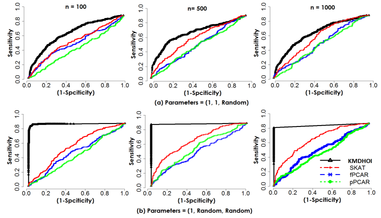
Figure 2: Receiver operating characteristics (ROC) of the kernel methods and relevant methods for higher order interaction detection with three sample sizes, $n\in\{100,500,1000\}$ for (a) third parameter value is random, (b) second and third parameter values are random. The sensitivity are plotted against (1- specificity) with the $p$-values threshold in the range zero to one $(0-1)$ with a step size $0.0001$.

5.4 Application to imaging genetics and epigenetics with schizophrenia

Here it is demonstrated the power of our proposed method and SKAT utilization for imaging genetic and epigenetic SZ data collected by MCIC. The key to integration, here, is to characterize the underlying interactions between the genetic features (gene-derived SNPs), human brain features (ROIs) and epigenetic features (gene-derived DNA methylation) with covariates (age, height, weight) on hippocampal volume derived from structural MRI scans of the SZ. To do this, we extracted significant (gene-derived SNPs)-ROI-(gene-derived DNA methylations) interactions using the proposed method and compared them to the SKAT methods.

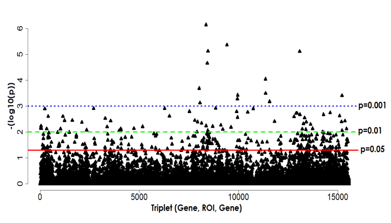
Figure 3: The plot of $-\rm{log}_{10}(p)$ with $15436$ triplets.

By considering $72$ genes-derived SNP, $116$ ROIs and $129$ gene-derived DNA methylation, we have $1077408\,(72\times 116\times 129)$ triplets. By the overall tests, we obtained $15436$ significant triplets at a $5\%$ level ($p$ $\leq 0.05$). Figure 3 visualizes the index plot of $-\rm{log}_{10}(p)$ for $15436$ triplets (the triplets in X-axis and $-\rm{log}_{10}(p)$ in Y-axis). The vertical solid, doted and double doted lines indicate the p-values at $0.05$, $0.01$, $0.001$, respectively. Based on these lines, we observed that $272$, $72$, and $13$ triplets are identified to have significantly higher order interactions at $0.05$, $0.01$ and $0.001$ levels, respectively.

Table 2 presents the ReML estimates of $\sigma^{2}$, $\tau^{(1)}$, $\tau^{(2)}$, $\tau^{(3)}$, $\tau^{(1\times 2)}$, $\tau^{(1\times 3)}$, $\tau^{(2\times 3)}$, $\tau^{(1\times 2\times 3)}$ and the $p$-values for the proposed and SKAT methods on each of the $13$ triplets, which are identified to have interaction significance at a level of $0.001$. At this $p$-value, we have $6$ gene-derives SNPs (IL1B, MAGI2, NRG1, PDLIM5, SLC18A1, TDRD3), $10$ ROIs (CRBL8.L, CRBLCrus1.L, ORBSUP.R, LING.L, CAU.R, IPL.L, IPL.R, PoCG.L, ITG.R, VER54), and 6 gene-derived DNA methylations (CRABP1, FBXO28, DUSP1, FHIT, PLAGL1, TFPI2) that have significant interaction effects on the hippocampal volume of SZ patients.

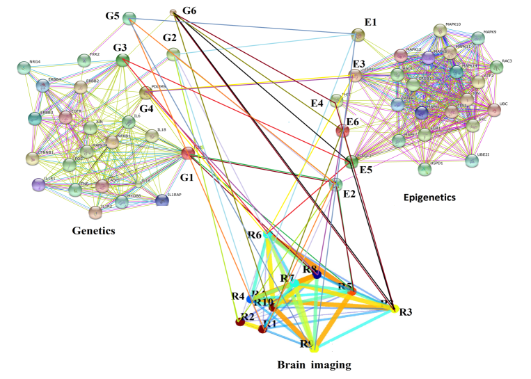
Figure 4: The network graph of features interaction of each individual view and features interactions of among others view ($p\leq 0.001$). Each node represents genes-derived SNP ( G1: IL1B, G2: MAGI2, G3: NRG1, G4: PDLIM5, G5: SLC18A1, G6: TDRD), ROIs (R1: CRBL8.L, R2: CRBLCrus1.L, R3: ORBSUP.R, R4: LING.L, R5: CAU.R, R6: IPL.L, R7: IPL.R, R8: PoCG.L, R9: ITG.R, R10: VER54) and gene-derived DNA methylation (E1: CRABP1, E2: FBXO28, E3: DUSP1, E4:FHIT, E5: PLAGL1, E6: TFPI2).

Figure 4 shows the network within each genetics, imaging and epigentics interactions as well as the interactions they have between all others views. Each node represents the gene-derived SNPs, ROIs and gene-derived DNA methylations, respectively. The interacting genes-derived SNPs, ROIs and gene-derived DNA methylations are connected with lines. The thickness of the connection line indicates the strength of the interaction among genes-derived SNPs, ROIs and gene-derived DNA methylations. These selected gene-derived SNPs and gene-derived DNA methylations show the interactions between several other genes. The selected ROIs also show the interaction within each selected ROI (shown in Figure 4) as well as the other ROIs (not shown in the figure). Following many studies in the literature, we have shown that each selected gene-derived SNPs our method has identified also has robust research discussing its role in the expression of SZ disease Siawa . (2016); Shibuya . (2013); Koide . (2013); Harrison  Law (206); Moselhy . (2015); Bly (2005).

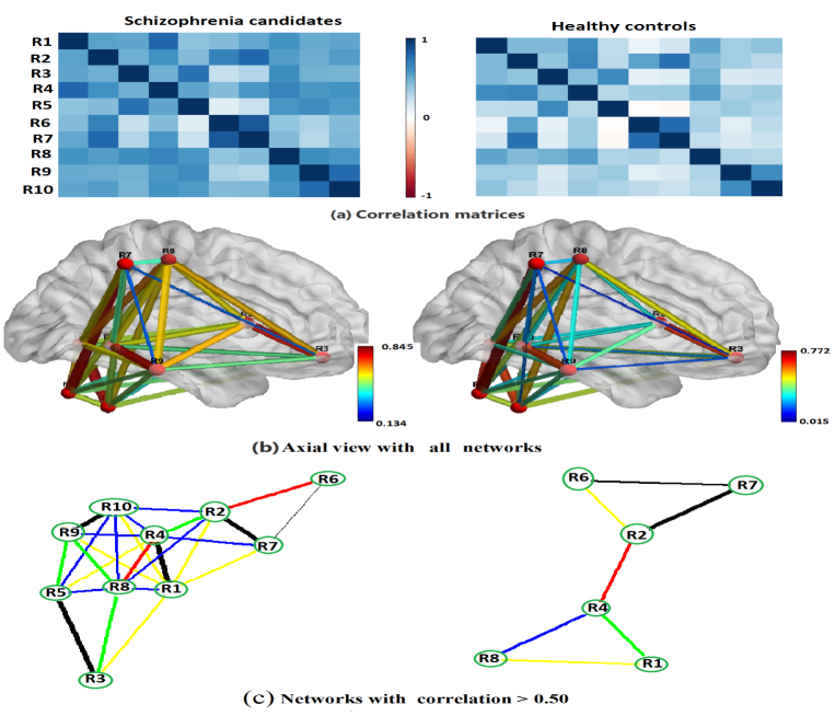
Figure 5: The visualization of selected $10$ ROIs for schizophrenia candidate and healthy control groups: (a) correlation matrices, (b) axial view with all networks, (c) networks with correlation $>0.5$.

Recent research has also shown that the $10$ ROIs selected by the proposed method have a critical role in brain related diseases Suk . (2016); Z. Chen . (2013); K. Wu . (2013). We additionally investigated the $10$ ROIs to confirm their role in SZ. To do this, each multidimensional variable ROI was converted to a univariate variable by taking the weighted mean. We then evaluated the differences between the SZ candidates and healthy controls using network measures and visualizations. Table 3 presents the transitivity, degree and global efficiency of each ROI for the SZ candidate and network and healthy control. From this table, we observed that the transitivity (measuring the probability that the adjacent vertices of a vertex are connected) of the SZ candidate group is larger than in the healthy control group (most of the ROIs and on average); this suggests that SZ tends to have more transitive triples. The degree (the number of edges incident to the vertex) of the SZ candidate group is larger than in the healthy control group for all of the ROIs; this indicates that these ROIs could have an impact on the SZ candidate. The global efficiency, the mean of all nodal efficiencies, of the SZ candidate group is different from the healthy control group. This may suggest that functional activity of the SZ candidate is not similar to the functional activity of the healthy control group in these regions. Figure 5 shows the visualization of correlation matrices, axial view with all networks and networks with correlation $>0.05$ for the SZ candidate and healthy control group. From Figure 5, it can be observed that the ROIs in the SZ candidate groups are more correlated and connected than the healthy control group. Therefore, with strong agreement, it has been shown that the selected ROIs have potential impact on the expression of SZ disease.

Table 4 lists the selected significant gene-derived SNP, ROIs and gene-derived DNA methylation using the proposed method (KMDHOI) and SKAT at a $p\leq 0.01$. We found that $31$ genes-derived SNP, $35$ ROIs and $20$ genes-derived DNA methylation from $72$ triplets were identified to have significance on the hippocampal volume of the SZ patients and the healthy controls. We also observed that $6$ gene-derived SNPs, $10$ ROIs and 6 gene-derived DNA methylations were significant at a $p\leq 0.001$. The underlined elements indicated in Table 4 have significant interaction triplets. Table  $5$ & $6$ (in the appendix) lists $72$ triplets, which were significant at a $p\leq 0.001$.

For the proposed KMDHOI approach, we considered triplets (gene-derived SNP, ROI, gene-derived DNA methylation) with a $p\leq 4^{-8}$ to be statistically significant after the Bonferroni correction for $1077408$ tests. Although the interaction (gene-derived SNP, ROI, gene-derived DNA methylation) results do not appear to be significant after adjusting for multiple comparisons, some of them appear promising consistent results. According to the $p-$values, we can determine the gene-derived SNPs, ROIs, and gene-derived DNA methylations that have a highly significant hippocampal volume on SZ patients and healthy controls. We observed gene-derived SNP (MAGI2, NRG1, SLC18A1, TDRD3), ROIs (CRBL8.L, CRBLCrus1.L, ORBSUP.R, LING.L, IPL.L, IPL.R) and gene-derived DNA methylations (CRABP1, FBXO28, FHIT, PLAGL1) at a $p\leq 0.0001$, gene-derived SNP (MAGI2, NRG1, TDRD3), ROIs (CRBL8.L, CRBLCrus1.L, IPL.L, IPL.R) and gene-derived DNA methylation (FBXO28, PLAGL1) at a $p\leq 0.00001$, and genes-derived SNP (MAGI2), ROIs (CRBLCrus1.L), and gene-derived DNA methylation (FBXO28) at a $p\leq 0.000001$, which are identified to have high interaction effects on hippocampal volume of SZ patients and healthy control.

To confirm this discovery, we used the DAVID, and gene ontology (GO) enrichment analysis to find the most relevant GO terms associated with the selected $31$ genes. The selected genes are associated with a set of annotation terms. We compared $5$ annotation categories, including literature, disease, gene ontology, pathways and protein interaction using DAVID Huang . (2009). Table  $7$ (in the appendix) presents five annotation categories of the $31$ selected genes. From this table, we observed that the selected genes have had remarkable literature review done in past studies. According to the disease annotation, the selected genes are highly associated with complex diseases including SZ, cognitive function, bipolar disorder, and others. By GO annotation, the selected genes have significant relationship to single-organism processes, response to stimuli, developmental processes and etc. From the table, we observed that the selected genes have a significant pathway to facilitate biological interpretation in a network context. Moreover, protein interaction annotations show that the selected genes have been discussed in many biomedical papers Sanders . (2008); Gerhard . (2004); Strausberg . (2002).

Genes do not function alone. Rather, they interact with each other. When genes share a similar set of GO annotation terms, they are most likely to be involved in similar biological mechanisms. To confirm this, we extracted the (gene-derived SNPs)-(gene-derived DNA methylations) network using STRING Szklarczyk . (2007). STRING imports protein association knowledge from databases of physical interaction and databases of curated biological pathway knowledge. In STRING, the simple interaction unit is the functional association (functional relationship between two proteins/ genes) that is most likely contributing to a common biological purpose. In this view, the color saturation of the edges represents the confidence score of a functional association. Further network analysis shows that the number of nodes, expected number of edges, number of edges, average node degree, clustering coefficient, PPI enrichment $p$-values are $51$, $93$, $300$, $11.8$, $0.603$, and $p\leq 0\times 10^{-16}$, respectively Szklarczyk . (2007). This network has significantly more interactions than expected. This means that these genes have more interactions among themselves than what would be expected for a random set of genes of similar size drawn from the genome. Such an enrichment indicates that the proteins/genes are at least biologically connected as a group.

Table 2: The selected significant genes-derived SNP, ROIs and gene-derived DNA methylation using the proposed method (KMDHOI) and SKAT. The $p-$values threshold was fixed to $0.001$.

			KMDHOI										SKAT
Genetics	Imaging	Epigenetics	$\sigma^{2}$	$\tau^{(1)}$	$\tau^{(2)}$	$\tau^{(3)}$	$\tau^{1\times 2}$	$\tau^{1\times 3}$	$\tau^{2\times 3}$	$\tau^{1\times 2\times 3}$	OVA	HOI	HOI
${\bf IL1B}$	${\bf CAU.R}$	${\bf FBXO28}$	$0.6755$	$0.0038$	$0.0229$	$0.1225$	$1.1013$	$0.0000$	$0.1307$	$1.3606$	$0.0383$	$2E-04$	$0.4943$
${\bf IL1B}$	${\bf PoCG.R}$	${\bf FBXO28}$	$0.5837$	$0.0189$	$0.1827$	$0.1247$	$1.8403$	$0.0000$	$0.3469$	$1.0603$	$0.0202$	$7E-04$	$0.2871$
${\bf MAGI2}$	${\bf CRBLCrus1.L}$	${\bf FBXO28}$	$0.1833$	$0.3246$	$0.0000$	$0.2693$	$1.1963$	$2.2426$	$1.3683$	$0.0100$	$0.0288$	$0E-06$	$0.01891$
${\bf MAGI2}$	${\bf LING.L}$	${\bf CRABP1}$	$0.1813$	$0.4366$	$0.0000$	$0.0885$	$1.5370$	$2.6299$	$1.0271$	$0.0100$	$0.0470$	$0E-05$	$0.4030$
${\bf MAGI2}$	${\bf IPL.R}$	${\bf FBXO28}$	$0.1833$	$0.3778$	$0.0000$	$0.3044$	$0.9808$	$2.3888$	$1.2203$	$0.0100$	$0.0457$	$0E-05$	$0.5592$
${\bf NRG1}$	${\bf IPL.L}$	${\bf PLAGL1}$	$0.3682$	$0.0024$	$0.2162$	$0.1270$	$1.1227$	$2.7930$	$0.0000$	$0.2056$	$0.0284$	$0E-05$	$0.6664$
${\bf PDLIM5}$	${\bf IPL.L}$	${\bf DUSP1}$	$0.3648$	$0.0000$	$0.0804$	$0.2182$	$1.5177$	$1.9409$	$1.0276$	$0.0100$	$0.0183$	$5E-04$	$0.0173$
${\bf PDLIM5}$	${\bf PoCG.R}$	${\bf DUSP1}$	$0.3598$	$0.0000$	$0.2256$	$0.0139$	$0.9189$	$1.7853$	$1.2796$	$0.0100$	$0.0498$	$Ee-04$	$0.2761$
${\bf SLC18A1}$	${\bf ORBsup.R}$	${\bf FHIT}$	$0.4096$	$0.0065$	$0.5356$	$0.2276$	$1.3456$	$0.0000$	$1.0003$	$0.1323$	$0.0495$	$1E-04$	$0.0522$
${\bf SLC18A1}$	${\bf ORBsup.R}$	${\bf PLAGL1}$	$0.2869$	$0.0000$	$0.3909$	$0.1933$	$1.0186$	$1.3148$	$1.3676$	$0.0100$	$0.0373$	$3E-04$	$0.0149$
${\bf SLC18A1}$	${\bf Vermis45}$	${\bf TFPI2}$	$0.5571$	$0.0447$	$0.0815$	$0.0020$	$0.0000$	$1.0458$	$0.5579$	$0.0100$	$0.0354$	$7E-04$	$0.4234$
${\bf TDRD3}$	${\bf CRBL8.L}$	${\bf FBXO28}$	$0.5856$	$0.2284$	$0.0022$	$0.0702$	$1.1722$	$0.7667$	$0.0000$	$0.0100$	$0.0052$	$0E-05$	$0.0807$
${\bf TDRD3}$	${\bf ITG.R}$	${\bf CRABP1}$	$0.5291$	$0.2318$	$0.0000$	$0.0223$	$0.7052$	$0.6038$	$0.6240$	$0.0100$	$0.0033$	$4E-04$	$0.0359$

Table 3: The network measurements (transitivity, degree, and global efficiency) of the selected $10$ ROIs for schizophrenia candidate and healthy control groups.

	Transitivity		Degree		Global efficiency
ROIs	Schizophrenia	Healthy	Schizophrenia	Healthy	Schizophrenia	Healthy
R1 = CRBL8.L	$0.571$	$1.000$	$7$	$2$	$0.800$	$0.317$
R2 = CRBLCrus1.L	$0.600$	$0.333$	$6$	$3$	$0.750$	$0.400$
R3 = ORBSUP.R	$0.667$	$0.000$	$3$	$1$	$0.5833$	$0.100$
R4 = LING.L	$0.667$	$0.333$	$7$	$3$	$0.800$	$0.400$
R5 = CAU.R	$0.700$	$0.000$	$5$	$1$	$0.683$	$0.100$
R6 = IPL.L	$1.000$	$1.000$	$2$	$2$	$0.500$	$0.317$
R7 = IPL.R	$0.667$	$1.000$	$4$	$2$	$0.650$	$0.317$
R8 = PoCG.L	$0.667$	$1.000$	$7$	$2$	$0.800$	$0.3167$
R9 = ITG.R	$0.900$	$0.000$	$5$	$1$	$0.683$	$0.100$
R10 = VER45	$0.800$	$0.000$	$6$	$1$	$0.750$	$0.100$

Table 4: The selected significant gene-derived SNPs, ROIs and gene-derived DNA methylations using the proposed method (KMDHOI) and SKAT at $p\leq 0.01$. The bold indicates significant at $p\leq 0.001$. Note: the name of ROI is given by the AAL template.

Genetics	IL1B	MAGI2	NRG1	PDLIM5	SLC18A1	TDRD3	BDNF	CHGA	CHGB	CLINT1
	COMTD1	DAOA	DISC1	DRD2	DTNBP1	ERBB4	GABBR1	GABRB2	GRIN2B	GRM3
	HTR2A	IL10RA	MAGI1	MICB	NOS1AP	NOTCH4	NR4A2	NUMBL	PLXNA2	PPP3CC
	SNAP29
Imaging	CRBL8.L	CRBLCrus1.L	ORBSUP.R	LING.L	CAU.R	IPL.L	IPL.R	PoCG.L	ITG.R	VER45
	AMYG.L	CRBL10.R	CRBL10.L	CRBL3.R	CRBL3.R	CRBL45.L	CRBL6.L	CRBL8.R	CRBLCrus2.R	CRBLCrus2.L
	DCG.R	DCG.L	PCG.R	ORBsup.L	ORBmid.R	LING.R	ROL.R	SMA.R	TPOsup.R	TPOsup.L
	STG.L	ITG.L	Vermis10	Vermis3	MTG.R
Epigenetic	CRABP1	FBXO28	DUSP1	FHIT	PLAGL1	TFPI2	CCND2	CDKN1A	EDNRB	ESR1
	EYA4	FEN1	GPSN2	HOXA9	HOXB4	PTGS2	RB1	SRF	WDR37	ZNF512

Lastly, we conducted standard logistic regression analysis with covariates of age, gender, and BMI on the outcome of SZ disease (SZ vs healthy control). We found that BMI is a significant covariate for the SZ vs healthy control at a $p\leq 0.0353$. Thus, BMI is one of the risk factors of SZ disease. For a BMI $\geq 25$, we considered the subject to be a high risk. Based on this risk, we divided the estimated higher order interaction effect $\hat{\mathbf{h}}_{\mathbf{M}^{(1)}\times\mathbf{M}^{(2)}\times\mathbf{M}^{(3)}}$ values into four regimes: SZ with high BMI risk, SZ with low BMI risk, healthy control with high BMI risk, and healthy control with low BMI risk. Figure 6 shows the boxplots of the estimated interaction effect within each of the four regimes for the most significant triplet (MAGI2, CRBLCrus1.L, and FBXO28). The small variation indicates a higher risk of the interaction effect (hippocampal volume). This figure shows that the SZ and BMI risks largely dominate the interaction effect (i.e., higher SZ and BMI risk associated with higher risk of interaction) and vice versa.

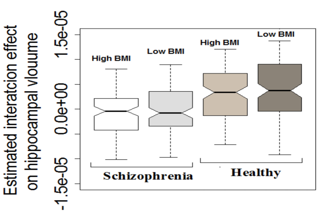
Figure 6: Boxplost of significant interaction effects in different regimes (SZ and high BMI risk, SZ and low BMI risk, healthy control and high BMI risk, healthy control and low BMI risk) for the most significant triplet (MAGI2, CRBLCrus1.L, FBXO28).

6 Discussion and future research

In this paper, we have proposed a semiparametric kernel method for higher order interactions between multiple data sets. Compared to the traditional PCA multiple regression and SKAT methods, the proposed method shows a more flexible and biological plausible way to model higher order epistasis among the genetic, imaging, and epigenetic data. While kernel based methods on multi-view data naturally produce more powerful and reproducible results, and are biologically more meaningful, the interpretation of model parameters is often challenging. Incorporating the gene and pathway analysis of biological information would facilitate additional improvements of model interpretation.

The performance of the proposed method was evaluated on both simulated and real MCIC data. The extensive simulation studies show evidence of the power gain of the proposed method relative to the alternative methods and suggest that the proposed methods perform remarkably better than the dimension reduction multiple regression and SKAT methods.

The utility of the proposed method is further demonstrated with the application to imaging genetics study of SZ. According to the $p-$values, the proposed method is able to rank the triplets (gene-derived SNPs)-ROI-(gene-derived DNA methylations) and subset of triplets can be selected which are highly related to SZ disease. At a $p\leq 0.01$ the proposed method extract the unique $31$ genes-derived SNP, $35$ ROIs and $20$ gene-derived DNA methylation from $72$ triplets, which are identified to have significant impact on hippocampal volume of SZ patients. By conducting gene ontology, pathway analysis, and several network measures including visualizations, we find evidence that the selected (gene-derived SNPs)- ROI-(gene-derived DNA methylations) have a significant influence on the manifestation of SZ disease. The identified triplets suggest that these statistical and biologically significant triplets may an important role in SZ related neurodegenerations. Our findings have indicated that genetic elements interplay with brain regions and epigenetic factors.

While we illustrated the proposed model using a quantitative hippocampal volume derived from structural MRI image phenotype, the utility of this model is that it can be applied to any phenotypes to detect higher order interactions in genetics, imaging, and epigenetic features, to include environmental covariates. The proposed model can also be extended to qualitative phenotypes for potentially widely applicable case-control studies (e.g., generalized kernel logistic regression).

It must be repeated that choosing a suitable kernel is indispensable. Kernel parameters may strongly influence the result desired for its application. Although the linear kernel does not have any free parameters, the linear kernel has certain limitations. Using the polynomial kernel makes it possible to detect higher order correlations. Polynomial kernels only map data into a finite dimensional space. In addition, both linear and polynomial kernels are unbounded. Many radial basis function kernels, such as the Gaussian kernel, map input data into an infinite dimensional space. The Gaussian kernel has a free parameter (bandwidth) but follows a number of properties (e.g., boundedness, consistency, universality, and robustness).

In this study, while we applied the median of the pairwise distance as a bandwidth for the Gaussian kernel, future studies might also compare the higher order interaction effects using a number of different kernels with different parameters, which may have broad implications to the detection of higher order interactions between disease phenotypes as described in the methods of this paper.

Acknowledgments

The authors wish to thank the NIH (R01 GM109068, R01 MH104680, ROI MH107354) and NSF EPSCoR program (1539067) for support.

Appendix

In the following sections, we present the details of the proposed method, Satterthwaite approximation to the score test, in addition we present supplementary tables and figures on our methods to their application to imaging genetics and epigenetics.

Appendix A Estimation of the linear mixed effect model using ReML

As discussed in the literature, we can estimate the variance components using the restricted maximum likelihood (ReML) approach Harville (1974); Lindstrom  Bates (1988). The restricted log-likelihood function of Eq. (13) is written as:

$$\ell_{R}(\boldsymbol{\theta})=-\frac{1}{2}ln(|\Theta(\boldsymbol{\theta})|)-\frac{1}{2}ln(|\mathbf{X}^{T}\mathbf{\Theta}^{-1}(\boldsymbol{\theta})\mathbf{X}|)-\frac{1}{2}(\mathbf{y}-\mathbf{X}\boldsymbol{\hat{\beta}})^{T}\boldsymbol{\Theta}^{-1}(\boldsymbol{\theta})(\mathbf{y}-\mathbf{X}\boldsymbol{\beta})$$ (A.1)

where $\boldsymbol{\hat{\beta}}$ is the BLUP of the regression coefficients $\boldsymbol{\beta})$ $\Theta(\boldsymbol{\theta})=\sigma^{2}\mathbf{I}+\tau^{(1)}\mathbf{K}^{(1)}+\tau^{(2)}\mathbf{K}^{(2)}+\tau^{(3)}\mathbf{K}^{(3)}+\tau^{(1\times 2)}\mathbf{K}^{(1\times 2)}+\tau^{(1\times 3)}\mathbf{K}^{(1\times 3)}+\tau^{(2\times 3)}\mathbf{K}^{(2\times 3)}+\tau^{(1\times 2\times 3)}\mathbf{K}^{(1\times 2\times 3)}$, where $\boldsymbol{\theta}=(\sigma^{2},\tau^{(1)},\tau^{(2)},\tau^{(3)},\tau^{1\times 2},\tau^{2\times 3},\tau^{1\times 2\times 3})$ are the variance components. To estimate the variance components, we need to perform the partial derivative of Eq. (A.1) with respective to each variance component:

$$\frac{\partial\ell_{R}}{\partial\boldsymbol{\theta}_{i}} = -\frac{1}{2}\rm{{\bf tr}}(\mathbf{W}\mathbf{G}_{i})+\frac{1}{2}(\mathbf{y}-\mathbf{X}\boldsymbol{\hat{\beta}})^{T}\boldsymbol{\Theta}^{-1}(\boldsymbol{\theta})\mathbf{G}_{i}\boldsymbol{\Theta}^{-1}(\boldsymbol{\theta})\mathbf{1}^{T}(\mathbf{y}-\mathbf{X}\boldsymbol{\beta})$$ (A.2)

$$= -\frac{1}{2}\rm{{\bf tr}}\left(\mathbf{W}\mathbf{G}_{i}\right)+\frac{1}{2}\mathbf{y}^{T}\mathbf{W}\mathbf{G}_{i}\mathbf{W}\mathbf{y}=0$$

where $\mathbf{G}_{i}=\frac{\partial\boldsymbol{\Theta}}{\boldsymbol{\theta}_{i}}$ and $\mathbf{W}=\boldsymbol{\Theta}^{-1}-\boldsymbol{\Theta}^{-1}\mathbf{X}(\mathbf{X}^{T}\boldsymbol{\Theta}^{-1}\mathbf{X})^{-1}\mathbf{X}^{T}\boldsymbol{\Theta}^{-1}$. We also have $\frac{\partial\boldsymbol{\Theta}}{\partial\sigma^{2}}=\mathbf{I}$,   $\frac{\partial\boldsymbol{\Theta}}{\partial\tau^{(1)}}=\mathbf{K}^{(1)}$,   $\frac{\partial\boldsymbol{\Theta}}{\partial\tau^{(2)}}=\mathbf{K}^{(2)}$,   $\frac{\partial\boldsymbol{\Theta}}{\partial\tau^{(3)}}=\mathbf{K}^{(3)}$,   $\frac{\partial\boldsymbol{\Theta}}{\partial\tau^{(1\times 2)}}=\mathbf{K}^{(1\times 2)}$,  $\frac{\partial\boldsymbol{\Theta}}{\partial\tau^{(1\times 3)}}=\mathbf{K}^{(1\times 3)}$,  $\frac{\partial\boldsymbol{\Theta}}{\partial\tau^{(1\times 2\times 3)}}=\mathbf{K}^{(1\times 2\times 3)}$. The $(i,j)$-th element of the observed and expected information matrices are

$$\left[\frac{\partial^{2}\ell_{R}}{\partial\boldsymbol{\theta}_{i}\partial\boldsymbol{\theta}_{j}}\right]_{ij}=-\frac{1}{2}\rm{{\bf tr}}(\mathbf{W}\mathbf{G}_{i}\mathbf{W}\mathbf{G}_{j})+\mathbf{y}^{T}\mathbf{W}\mathbf{G}_{i}\mathbf{W}\mathbf{G}_{i}\mathbf{W}\mathbf{y},$$

$$\rm{\mathbf{E}}\left[\frac{\partial^{2}\ell_{R}}{\partial\boldsymbol{\theta}_{i}\partial\boldsymbol{\theta}_{j}}\right]_{ij}=-\frac{1}{2}\rm{{\bf tr}}(\mathbf{W}\mathbf{G}_{i}\mathbf{W}\mathbf{G}_{j})=\mathcal{I}(\boldsymbol{\theta}),$$

respectively. Using Fisher’s scoring algorithm (Newton-Raphson method to solve maximum likelihood equations numerically), given an initial value of unknown parameters at the $h$-th iteration $\boldsymbol{\theta}_{(k+1)}$, the parameters are updated as

$$\boldsymbol{\theta}_{(k+1)}=\boldsymbol{\theta}_{(k)}+[\mathcal{I}(\boldsymbol{\theta}^{-1}_{(h)}][\frac{\partial\ell_{R}}{\partial\boldsymbol{\theta}}]_{\boldsymbol{\theta}_{(k)}}.$$

In expectation maximization (EM) algorithm, we used a set of initial points ($0$, $0.00001$, $0.0001$, $0.001$, $0.01$, $0.1$, $1$) of the variance components for the optimization algorithm and chose the best one (maximized ReML) to avoid the local minim Laid . (1987). For the $\sigma^{2}$, we fixed initial values to $\rm{Var}(\mathbf{y})$. After EM update, we then conducted the Fisher’s scoring algorithm for the left iterations until the difference between successive log ReML values ($|\ell_{R(h+1)}-\ell_{R(h)}|$) was smaller than $10^{-05}$. In most cases the ReML algorithm converged in less than $50$ iterations and in some cases it converged very quickly with $10$ iterations, taking only a few seconds with an R-program.

Appendix B Satterthwaite approximation to the score test

The restricted score function under the null hypothesis $H_{0}:\tau^{(1)}=\tau^{(2)}=\tau^{(3)}=\tau^{(1\times 2)}=\tau^{(1\times 3)}=\tau^{(2\times 3)}=\tau^{(1\times 2\times 3)}=0$ is given by:

$$\frac{\partial\ell_{R}}{\partial\boldsymbol{\theta}_{i}}\big{|}_{\boldsymbol{\tau}=0}=-\frac{1}{2\sigma^{2}}\rm{{\bf tr}}\left(\mathbf{W}_{0}\mathbf{G}_{i}\right)+\frac{1}{2\sigma^{4}}(\mathbf{y}-\mathbf{X}\boldsymbol{\hat{\beta}})^{T}\boldsymbol{\Theta}^{-1}\mathbf{G}_{i}(\mathbf{y}-\mathbf{X}\boldsymbol{\beta})$$ (B.1)

where $\mathbf{W}_{0}=\mathbf{I}-\mathbf{I}(\mathbf{I}^{T}\mathbf{I})^{-1}\mathbf{I}^{T}$ and $\boldsymbol{\tau}=\tau^{(1)}=\tau^{(2)}=\tau^{(3)}=\tau^{(1\times 2)}=\tau^{(1\times 3)}=\tau^{(2\times 3)}$. Since the MLE is $\sqrt{n}$ consistent, the asymptotic distribution of $S(\hat{\sigma}_{0}^{2})$ can still be approximated by the scaled chi-square distribution. By considering the true value of $\sigma^{2}$ under null hypothesis as $\sigma^{2}_{0}$, the mean and variance of the test statistic $S(\hat{\sigma}_{0}^{2})$ are:

$$\rm{E}[S(\sigma_{0}^{2})]=\frac{1}{2}\rm{{\bf tr}}\left(\mathbf{W}_{0}\mathbf{K}\right)=\rm{E}[\gamma\chi^{2}_{\nu}]=\gamma\nu,\rm{and}$$

$$\rm{Var}[S(\sigma_{0}^{2})]=\frac{1}{2}\rm{{\bf tr}}\left(\mathbf{W}_{0}\mathbf{K}\mathbf{W}_{0}\mathbf{K}\right)=\rm{Var}[\gamma\chi^{2}\nu]=2\gamma^{2}\nu$$

where $\mathbf{K}=\mathbf{K}^{(1)}+\mathbf{K}^{(2)}+\mathbf{K}^{(3)}+\mathbf{K}^{(1\times 2)}+\mathbf{K}^{(1\times 3)}+\mathbf{K}^{(2\times 3)}+\mathbf{K}^{(1\times 2\times 3)}$ and $\hat{\boldsymbol{\beta}}$. To account for this substitution, we need to estimate $\gamma$ and $\nu$ by replacing the $\rm{Var}[S(\hat{\sigma}_{0}^{2})]$ based on the efficient information. The elements of the Fisher information matrix $\boldsymbol{\tau}$ are written as:

$$\scalebox{0.75}{\mbox{$\displaystyle\mathcal{I}_{\boldsymbol{\tau}\boldsymbol{\tau}}=\begin{bmatrix}\rm{{\bf tr}}(\mathbf{A}^{(1)}\mathbf{A}^{(1)})&\rm{{\bf tr}}(\mathbf{A}^{(1)}\mathbf{A}^{(2)})&\rm{{\bf tr}}(\mathbf{A}^{(1)}\mathbf{A}^{(3)})&\rm{{\bf tr}}(\mathbf{A}^{(1)}\mathbf{A}^{(1\times 2)})&\rm{{\bf tr}}(\mathbf{A}^{(1)}\mathbf{A}^{(1\times 3)})&\rm{{\bf tr}}(\mathbf{A}^{(1)}\mathbf{A}^{(2\times 3)})&\rm{{\bf tr}}(\mathbf{A}^{(1)}\mathbf{A}^{(1\times 2\times 3)})\\ \rm{{\bf tr}}(\mathbf{A}^{(2)}\mathbf{A}^{(1)})&\rm{{\bf tr}}(\mathbf{A}^{(2)}\mathbf{A}^{(2)})&\rm{{\bf tr}}(\mathbf{A}^{(2)}\mathbf{A}^{(3)})&\rm{{\bf tr}}(\mathbf{A}^{(2)}\mathbf{A}^{(1\times 2)})&\rm{{\bf tr}}(\mathbf{A}^{(2)}\mathbf{A}^{(1\times 3)})&\rm{{\bf tr}}(\mathbf{A}^{(2)}\mathbf{A}^{(2\times 3)})&\rm{{\bf tr}}(\mathbf{A}^{(2)}\mathbf{A}^{(1\times 2\times 3)})\\ \rm{{\bf tr}}(\mathbf{A}^{(3)}\mathbf{A}^{(1)})&\rm{{\bf tr}}(\mathbf{A}^{(3)}\mathbf{A}^{(2)})&\rm{{\bf tr}}(\mathbf{A}^{(3)}\mathbf{A}^{(3)})&\rm{{\bf tr}}(\mathbf{A}^{(3)}\mathbf{A}^{(1\times 2)})&\rm{{\bf tr}}(\mathbf{A}^{(3)}\mathbf{A}^{(1\times 3)})&\rm{{\bf tr}}(\mathbf{A}^{(3)}\mathbf{A}^{(2\times 3)})&\rm{{\bf tr}}(\mathbf{A}^{(3)}\mathbf{A}^{(1\times 2\times 3)})\\ \rm{{\bf tr}}(\mathbf{A}^{(1\times 2)}\mathbf{A}^{(1)})&\rm{{\bf tr}}(\mathbf{A}^{(1\times 2)}\mathbf{A}^{(2)})&\rm{{\bf tr}}(\mathbf{A}^{(1\times 2)}\mathbf{A}^{(3)})&\rm{{\bf tr}}(\mathbf{A}^{(1\times 2)}\mathbf{A}^{(1\times 2)})&\rm{{\bf tr}}(\mathbf{A}^{(1\times 2)}\mathbf{A}^{(1\times 3)})&\rm{{\bf tr}}(\mathbf{A}^{(1\times 2)}\mathbf{A}^{(2\times 3)})&\rm{{\bf tr}}(\mathbf{A}^{(1\times 2)}\mathbf{A}^{(1\times 2\times 3)})\\ \rm{{\bf tr}}(\mathbf{A}^{(1\times 3)}\mathbf{A}^{(1)})&\rm{{\bf tr}}(\mathbf{A}^{(1\times 3)}\mathbf{A}^{(2)})&\rm{{\bf tr}}(\mathbf{A}^{(1\times 3)}\mathbf{A}^{(3)})&\rm{{\bf tr}}(\mathbf{A}^{(1\times 3)}\mathbf{A}^{(1\times 2)})&\rm{{\bf tr}}(\mathbf{A}^{(1\times 3)}\mathbf{A}^{(1\times 3)})&\rm{{\bf tr}}(\mathbf{A}^{(1\times 3)}\mathbf{A}^{(2\times 3)})&\rm{{\bf tr}}(\mathbf{A}^{(1\times 3)}\mathbf{A}^{(1\times 2\times 3)})\\ \rm{{\bf tr}}(\mathbf{A}^{(2\times 3)}\mathbf{A}^{(1)})&\rm{{\bf tr}}(\mathbf{A}^{(2\times 3)}\mathbf{A}^{(2)})&\rm{{\bf tr}}(\mathbf{A}^{(2\times 3)}\mathbf{A}^{(3)})&\rm{{\bf tr}}(\mathbf{A}^{(2\times 3)}\mathbf{A}^{(1\times 2)})&\rm{{\bf tr}}(\mathbf{A}^{(2\times 3)}\mathbf{A}^{(1\times 3)})&\rm{{\bf tr}}(\mathbf{A}^{(2\times 3)}\mathbf{A}^{(2\times 3)})&\rm{{\bf tr}}(\mathbf{A}^{(2\times 3)}\mathbf{A}^{(1\times 2\times 3)})\\ \rm{{\bf tr}}(\mathbf{A}^{(1\times 2\times 3)}\mathbf{A}^{(1)})&\rm{{\bf tr}}(\mathbf{A}^{(1\times 2\times 3)}\mathbf{A}^{(2)})&\rm{{\bf tr}}(\mathbf{A}^{(1\times 2\times 3)}\mathbf{A}^{(3)})&\rm{{\bf tr}}(\mathbf{A}^{(1\times 2\times 3)}\mathbf{A}^{(1\times 2)})&\rm{{\bf tr}}(\mathbf{A}^{(1\times 2\times 3)}\mathbf{A}^{(1\times 3)})&\rm{{\bf tr}}(\mathbf{A}^{(1\times 2\times 3)}\mathbf{A}^{(2\times 3)})&\rm{{\bf tr}}(\mathbf{A}^{(1\times 2\times 3)}\mathbf{A}^{(1\times 2\times 3)})\\ \end{bmatrix}$}},$$

$$\scalebox{0.75}{\mbox{$\displaystyle\mathcal{I}_{\boldsymbol{\tau}\sigma^{2}}=\frac{1}{2}[\rm{{\bf tr}}(\mathbf{A}^{(1)})\qquad\rm{{\bf tr}}(\mathbf{A}^{(2)})\qquad\rm{{\bf tr}}(\mathbf{A}^{(1)})\qquad\rm{{\bf tr}}(\mathbf{A}^{(1\times 2)})\qquad\rm{{\bf tr}}(\mathbf{A}^{(1\times 3)})\qquad\rm{{\bf tr}}(\mathbf{A}^{(2\times 3)})\qquad\rm{{\bf tr}}(\mathbf{A}^{(1\times 2\times 3)}$}}],$$

and $\mathcal{I}_{\sigma^{2}\sigma^{2}}=\frac{1}{2}\rm{{\bf tr}}(\mathbf{W}_{0}\mathbf{W}_{0})$, where $\mathbf{A}^{(1)}=\mathbf{W}_{0}\mathbf{K}^{(1)}$,  $\mathbf{A}^{(2)}=\mathbf{W}_{0}\mathbf{K}^{(2)}$,  $\mathbf{A}^{(3)}=\mathbf{W}_{0}\mathbf{K}^{(3)}$,   $\mathbf{A}^{(1\times 2)}=\mathbf{W}_{0}\mathbf{K}^{(1\times 2)}$,  $\mathbf{A}^{(1\times 3)}=\mathbf{W}_{0}\mathbf{K}^{(1\times 3)},$  $\mathbf{A}^{(2\times 3)}=\mathbf{W}_{0}\mathbf{K}^{(2\times 3)}$,  $\mathbf{A}^{(1\times 2\times 3)}=\mathbf{W}_{0}\mathbf{K}^{(1\times 2\times 3)}$. Using these information matrices, we have the efficient information $\tilde{\mathcal{I}}_{\boldsymbol{\tau}\boldsymbol{\tau}}=\mathcal{I}_{\boldsymbol{\tau},\boldsymbol{\tau}}-\mathcal{I}_{\boldsymbol{\tau}\sigma^{2}}^{T}\mathcal{I}_{\sigma^{2}\sigma^{2}}^{-1}\mathcal{I}_{\boldsymbol{\tau}\sigma^{2}}$ and $\rm{Var}[S(\hat{\sigma}_{0}^{2})]=\rm{SUM}[\tilde{\mathcal{I}}_{\boldsymbol{\tau}\boldsymbol{\tau}}]$, where the operator ”SUM” indicates the sum of all the element in the matrix. By considering the adjusted parameters $\hat{\gamma}=\frac{\rm{Var}[S(\hat{\sigma}_{0}^{2})]}{2\rm{E}[S(\sigma_{0}^{2})]}$ and $\hat{\nu}=\frac{2\rm{E}[S(\sigma_{0}^{2})^{2}]}{\rm{Var}[S(\hat{\sigma}_{0}^{2})]}$, the $p-$value of an experimental score statistic $S(\hat{\sigma}_{0}^{2})$ is obtained using the scaled chi-square distribution $\hat{\gamma}\chi^{2}_{\hat{\nu}}$.

The score test statistic $S_{\rm{I}}(\tilde{\tau_{\rm{I}}})$ defined in Eq. (16) for the higher order interaction effect that testing the null hypothesis $H_{0}:\tau^{(1\times 2\times 3)}=0$ is approximated by a scaled chi-square distribution $\hat{\gamma}_{\rm{I}}\chi^{2}_{\hat{\nu_{I}}}$. To do this, let $\Sigma=\sigma^{2}\mathbf{I}+\tau^{(1)}\mathbf{K}^{(1)}+\tau^{(2)}\mathbf{K}^{(2)}+\tau^{(3)}\mathbf{K}^{(3)}+\tau^{1\times 2}\mathbf{K}^{(1\times 2)}+\tau^{(1\times 3)}\mathbf{K}^{(1\times 3)}+\tau^{(2\times 3)}\mathbf{K}^{(2\times 3)}$, and $\tau^{(1)},\tau^{(2)},\tau^{(3)},\tau^{(1\times 2)},\tau^{(1\times 3)},\tau^{(2\times 3)}$, and $\sigma^{2}$ are model parameters under the null model $\mathbf{y}=\mathbf{X}\boldsymbol{\beta}+\mathbf{h}_{\mathbf{M}^{(1)}}+\mathbf{h}_{\mathbf{M}^{(2)}}+\mathbf{h}_{\mathbf{M}^{(3)}}+\mathbf{h}_{\mathbf{M}^{(1)}\times\mathbf{M}^{(2)}}+\mathbf{h}_{\mathbf{M}^{(1)}\times\mathbf{M}^{(3)}}+\boldsymbol{\epsilon}$. The score function Eq. (A.1) under the null hypothesis becomes

$$\frac{\partial\ell_{R}}{\partial\tau^{(1\times 2\times 3)}}\big{|}_{\tau^{(1\times 2\times 3)}=0} = -\frac{1}{2\sigma^{2}}[\rm{{\bf tr}}\left(\mathbf{W}_{01}\mathbf{K}^{(1\times 2\times 3)}\right)-(\mathbf{y}-\mathbf{X}\boldsymbol{\hat{\beta}})^{T}\mathbf{\Sigma}^{-1}\mathbf{K}^{(1\times 2\times 3)}\mathbf{\Sigma}^{-1}(\mathbf{y}-\mathbf{X}\boldsymbol{\beta})]$$ (B.2)

$$= -\frac{1}{2}[\rm{{\bf tr}}\left(\mathbf{W}_{01}\mathbf{K}^{(1\times 2\times 3)}\right)-\mathbf{y}^{T}\mathbf{W}_{01}\mathbf{K}^{(1\times 2\times 3)}\mathbf{W}_{01}\mathbf{y})$$

where $\mathbf{W}_{01}=\Sigma^{-1}-\Sigma^{-1}\mathbf{X}(\mathbf{X}^{T}\Sigma^{-1}\mathbf{X})^{-1}\mathbf{X}^{T}\Sigma^{-1}$ is the projection matrix under the null hypothesis. The test statistic for the higher order interaction effect is as follows:

$$S_{\rm{I}}(\boldsymbol{\tau}_{\rm{I}})=\frac{1}{2\sigma^{2}_{0}}\mathbf{y}^{T}\mathbf{W}_{01}\mathbf{K}^{(1\times 2\times 3)}\mathbf{W}_{01}\mathbf{y},$$

where $\boldsymbol{\tau}_{\rm{I}}=(\tau^{(1)},\tau^{(2)},\tau^{(3)},\tau^{(1\times 2)}).$ Similarly for overall effect test, we can use the Satterthwaite method to approximate the distribution of higher order intersection test statistic $S_{\rm{I}}(\tau_{\rm{I}})$ by a scaled chi-square distribution with a scaled $\gamma_{\rm{I}}$ and degree of freedom $\nu_{\rm{I}}$, i.e., $S_{\rm{I}}(\tau_{\rm{I}})\sim\gamma_{\rm{I}}\chi^{2}_{\nu_{\rm{I}}}$. The mean and variance of the test statistic $S_{\rm{I}}(\boldsymbol{\tau}_{\rm{I}})$ are:

$$\rm{E}[S_{\rm{I}}(\boldsymbol{\tau}_{\rm{I}})]=\frac{1}{2}\rm{{\bf tr}}\left(\mathbf{W}_{01}\mathbf{K}^{(1\times 2\times 3)}\right)=\rm{E}[\gamma_{\rm{I}}\chi^{2}_{\nu_{\rm{I}}}]=\gamma_{\rm{I}}\nu_{\rm{I}},\rm{and}$$

$$\rm{Var}[S_{\rm{I}}(\boldsymbol{\tau}_{\rm{I}})]=\frac{1}{2}\rm{{\bf tr}}\left(\mathbf{W}_{0}\mathbf{K}^{(1\times 2\times 3)}\mathbf{W}_{0}\mathbf{K}^{(1\times 2\times 3)}\right)=\rm{Var}[\gamma_{\rm{I}}\chi^{2}_{\nu_{\rm{I}}}]=2\gamma_{\rm{I}}^{2}\nu_{\rm{I}}$$

where $\mathbf{K}=\mathbf{K}^{(1)}+\mathbf{K}^{(2)}+\mathbf{K}^{(3)}+\mathbf{K}^{(1\times 2)}+\mathbf{K}^{(1\times 3)}+\mathbf{K}^{(2\times 3)}+\mathbf{K}^{(1\times 2\times 3)}$, $\gamma_{\rm{I}}=\frac{\rm{Var}[S_{\rm{I}}(\boldsymbol{\tau}_{\rm{I}}]}{2\rm{E}[S_{\rm{I}}(\boldsymbol{\tau}_{\rm{I}}]}$ and $\nu_{\rm{I}}=\frac{2\rm{E}[S_{\rm{I}}(\boldsymbol{\tau}_{\rm{I}}]}{\rm{Var}[S_{\rm{I}}(\boldsymbol{\tau}_{\rm{I}}]}$, receptively. In practice, the unknown model parameters $\tau^{(1)},\tau^{(2)},\tau^{(3)},\tau^{(1\times 2)},\tau^{(1\times 3)},\tau^{(2\times 3)}$, and $\sigma^{2}$ are estimated by their respective ReML estimates $\hat{\tau}^{(1)},\hat{\tau}^{(2)},\hat{\tau}^{(3)},\hat{\tau}^{(1\times 2)},\hat{\tau}^{(1\times 3)},\hat{\tau}^{(2\times 3)}$, and $\hat{\sigma}^{2}$ under the null hypothesis. The scaled parameter and degree of freedom are estimated by the MOM. Specifically, $\hat{\gamma}_{\rm{I}}=\frac{\widehat{\rm{Var}[S_{\rm{I}}(\boldsymbol{\tau}_{\rm{I}})]}}{2\widehat{\rm{E}[S_{\rm{I}}(\boldsymbol{\tau}_{\rm{I}})]}},$ and $\hat{\nu}_{\rm{I}}=\frac{2\widehat{\rm{E}[S_{\rm{I}}(\boldsymbol{\tau}_{\rm{I}})]}}{\widehat{\rm{Var}[S_{\rm{I}}(\boldsymbol{\tau}_{\rm{I}})]}}$, where $\widehat{\rm{E}[S_{\rm{I}}(\boldsymbol{\tau}_{\rm{I}})]}=\frac{1}{2}\rm{{\bf tr}}\left(\mathbf{W}_{01}\mathbf{K}^{(1\times 2\times 3)}\right)$ and $\widehat{\rm{Var}[S_{\rm{I}}(\boldsymbol{\tau}_{\rm{I}})]}=\frac{1}{2}\rm{{\bf tr}}\left(\mathbf{W}_{0}\mathbf{K}^{(1\times 2\times 3)}\mathbf{W}_{0}\mathbf{K}^{(1\times 2\times 3)}\right)-\frac{\boldsymbol{\Delta}\boldsymbol{\xi}^{-1}\boldsymbol{\Delta}}{2}$, in which

where $\mathbf{B}^{(1)}=\mathbf{W}_{01}\mathbf{K}^{(1)}$,  $\mathbf{B}^{(2)}=\mathbf{W}_{01}\mathbf{K}^{(2)}$,  $\mathbf{B}^{(3)}=\mathbf{W}_{01}\mathbf{K}^{(3)}$,   $\mathbf{B}^{(1\times 2)}=\mathbf{W}_{01}\mathbf{K}^{(1\times 2)}$,  $\mathbf{B}^{(1\times 3)}=\mathbf{W}_{01}\mathbf{K}^{(1\times 3)},$  $\mathbf{B}^{(2\times 3)}=\mathbf{W}_{01}\mathbf{K}^{(2\times 3)}$,  $\mathbf{B}^{(1\times 2\times 3)}=\mathbf{W}_{01}\mathbf{K}^{(1\times 2\times 3)}$. The $p-$value of an observed higher order interaction effect test score statistic $S_{\rm{I}}(\tau_{\rm{I}})$ is obtained using the scaled chi-square distribution $\hat{\gamma}_{\rm{I}}\chi^{2}_{\hat{\nu_{\rm{I}}}}$.

Appendix C Supplementary figures and tables

Table 5: The selected significant genes-derived SNP, ROIs and gene-derived DNA methylation using the proposed method (KMDHOI). The $p-$values threshold was fixed to $0.01$.

			KMDHOI
Genetics	Imaging	Epigenetics	$\sigma^{2}$	$\tau^{(1)}$	$\tau^{(2)}$	$\tau^{(3)}$	$\tau^{1\times 2}$	$\tau^{1\times 3}$	$\tau^{2\times 3}$	$\tau^{1\times 2\times 3}$	OVA	HOI
${\bf BDNF}$	${\bf AMYG.L}$	${\bf DUSP1}$	$0.5658$	$0.0559$	$0.0887$	$0.0041$	$0.0494$	$2.1147$	$0.0000$	$0.0100$	$0.0345$	$0.0069$
${\bf BDNF}$	${\bf CRBL10.L}$	${\bf FBXO28}$	$0.5589$	$0.0334$	$0.1414$	$0.0157$	$1.2657$	$0.0000$	$0.2034$	$0.0100$	$0.0102$	$0.0058$
${\bf BDNF}$	${\bf CRBL3.R}$	${\bf DUSP1}$	$0.4255$	$0.2077$	$0.0000$	$0.0556$	$0.7339$	$2.1418$	$1.0345$	$0.0100$	$0.0414$	$0.0072$
${\bf BDNF}$	${\bf ORBsup.L}$	${\bf FBXO28}$	$0.5515$	$0.0033$	$0.4506$	$0.0535$	$0.8534$	$0.6955$	$0.0000$	$0.0100$	$0.0078$	$0.0013$
${\bf BDNF}$	${\bf LING.R}$	${\bf CRABP1}$	$0.5510$	$0.5258$	$0.2416$	$0.0640$	$0.9032$	$0.7442$	$0.0000$	$0.0100$	$0.0114$	$0.0074$
${\bf BDNF}$	${\bf IPL.R}$	${\bf FBXO28}$	$0.4471$	$0.0388$	$0.1458$	$0.0644$	$1.2503$	$2.3689$	$0.0000$	$1.9045$	$0.0367$	$0.0024$
${\bf CHGA}$	${\bf AMYG.L}$	${\bf HOXA9}$	$0.4326$	$0.0027$	$0.3130$	$0.3598$	$1.5185$	$0.0000$	$1.1948$	$0.7093$	$0.0474$	$0.0075$
${\bf CHGB}$	${\bf CRBL3.L}$	${\bf DUSP1}$	$0.6779$	$0.0321$	$0.1444$	$0.1232$	$0.2505$	$0.5545$	$0.0000$	$0.0100$	$0.0454$	$0.0025$
${\bf CHGB}$	${\bf DCG.L}$	${\bf DUSP1}$	$0.5253$	$0.0247$	$0.0213$	$0.0570$	$1.2794$	$1.0467$	$0.0000$	$0.0100$	$0.0408$	$0.0035$
${\bf CHGB}$	${\bf STG.L}$	${\bf DUSP1}$	$0.5415$	$0.1053$	$0.0360$	$0.0017$	$1.1720$	$1.2059$	$0.0000$	$0.0100$	$0.0293$	$0.0035$
${\bf CLINT1}$	${\bf IPL.R}$	${\bf GPSN2}$	$0.4074$	$0.6728$	$0.0404$	$0.0514$	$1.2476$	$1.6953$	$0.0000$	$0.0100$	$0.0228$	$0.0042$
${\bf COMTD1}$	${\bf ROL.R}$	${\bf FBXO28}$	$0.5717$	$0.0740$	$0.0095$	$0.0479$	$2.5561$	$0.3378$	$0.0000$	$2.3490$	$0.0370$	$0.0083$
${\bf DAOA}$	${\bf ORBsup.L}$	${\bf DUSP1}$	$0.3721$	$0.1079$	$0.0731$	$0.0097$	$0.5586$	$3.5344$	$0.0000$	$0.0100$	$0.0490$	$0.0012$
${\bf DISC1}$	${\bf IPL.R}$	${\bf PLAGL1}$	$0.3370$	$0.0161$	$0.0547$	$0.1417$	$1.5286$	$3.2871$	$0.0000$	$1.4004$	$0.0439$	$0.0029$
${\bf DRD2}$	${\bf ORBsup.R}$	${\bf DUSP1}$	$0.3772$	$0.0000$	$0.3189$	$0.0073$	$1.1268$	$2.0353$	$0.9757$	$0.0100$	$0.0445$	$0.0062$
${\bf DTNBP1}$	${\bf IPL.R}$	${\bf SRF}$	$0.3940$	$0.1987$	$0.0637$	$0.2312$	$1.4537$	$1.8458$	$0.0000$	$0.0100$	$0.0267$	$0.0037$
${\bf ERBB4}$	${\bf CRBLCrus2.R}$	${\bf DUSP1}$	$0.2576$	$0.0000$	$0.0413$	$0.0401$	$1.2244$	$3.1904$	$1.0830$	$0.0100$	$0.0459$	$0.0088$
${\bf ERBB4}$	${\bf IPL.R}$	${\bf FEN1}$	$0.4484$	$0.0000$	$0.0762$	$0.0357$	$0.8799$	$2.9942$	$0.1061$	$0.0100$	$0.0294$	$0.0074$
${\bf ERBB4}$	${\bf IPL.R}$	${\bf HOXB4}$	$0.3308$	$0.6704$	$0.0669$	$0.0222$	$2.3489$	$1.9820$	$0.0000$	$0.0100$	$0.0396$	$0.0082$
${\bf GABBR1}$	${\bf LING.R}$	${\bf CRABP1}$	$0.5610$	$0.0068$	$0.4045$	$0.0563$	$1.8524$	$0.0000$	$0.7076$	$0.0100$	$0.0166$	$0.0072$
${\bf GABRB2}$	${\bf SMA.R}$	${\bf EDNRB}$	$0.5276$	$0.0139$	$0.1276$	$0.0364$	$1.3359$	$2.4832$	$0.0000$	$2.0971$	$0.0283$	$0.0061$
${\bf GRIN2B}$	${\bf IPL.R}$	${\bf HOXB4}$	$0.3523$	$0.2359$	$0.0352$	$0.0297$	$2.1599$	$2.1357$	$0.0000$	$0.0100$	$0.0421$	$0.0012$
${\bf GRM3}$	${\bf SMA.R}$	${\bf EYA4}$	$0.6435$	$0.0088$	$0.3928$	$0.0384$	$0.5390$	$1.5425$	$0.0000$	$0.4976$	$0.0237$	$0.0024$
${\bf HTR2A}$	${\bf ITG.L}$	${\bf FBXO28}$	$0.4496$	$0.3074$	$0.0087$	$0.0970$	$0.1874$	$2.0080$	$0.0000$	$0.0100$	$0.0211$	$0.0016$
${\bf IL10RA}$	${\bf LING.L}$	${\bf CRABP1}$	$0.5128$	$0.1846$	$0.1055$	$0.0436$	$1.3817$	$0.0000$	$0.1076$	$0.0100$	$0.0373$	$0.0035$
${\bf IL10RA}$	${\bf TPOsup.R}$	${\bf CRABP1}$	$0.5644$	$0.2024$	$0.0000$	$0.0364$	$1.3936$	$1.1762$	$0.0700$	$0.0100$	$0.0425$	$0.0098$
${\bf IL1B}$	${\bf AMYG.L}$	${\bf FBXO28}$	$0.5708$	$0.0130$	$0.4484$	$0.0755$	$1.8572$	$0.0000$	$0.3580$	$1.0757$	$0.0445$	$0.0040$
${\bf IL1B}$	${\bf CAU.R}$	${\bf FBXO28}$	$0.6755$	$0.0038$	$0.0229$	$0.1225$	$1.1013$	$0.0000$	$0.1307$	$1.3606$	$0.0383$	$0.0002$
${\bf IL1B}$	${\bf PoCG.R}$	${\bf FBXO28}$	$0.5837$	$0.0189$	$0.1827$	$0.1247$	$1.8403$	$0.0000$	$0.3469$	$1.0603$	$0.0202$	$0.0007$
${\bf MAGI1}$	${\bf CRBL6.L}$	${\bf CRABP1}$	$0.3178$	$0.5873$	$0.0201$	$0.0249$	$1.7962$	$1.7014$	$0.0000$	$0.0100$	$0.0346$	$0.0045$
${\bf MAGI2}$	${\bf CRBLCrus1.L}$	${\bf FBXO28}$	$0.1833$	$0.3246$	$0.0000$	$0.2693$	$1.1963$	$2.2426$	$1.3683$	$0.0100$	$0.0288$	$0.0000$
${\bf MAGI2}$	${\bf DCG.R}$	${\bf FBXO28}$	$0.3211$	$0.0000$	$0.1485$	$0.0513$	$2.0150$	$2.5252$	$0.3083$	$0.0100$	$0.0298$	$0.0057$

Table 6: Table $5$ continued:

			KMDHOI
Genetics	Imaging	Epigenetics	$\sigma^{2}$	$\tau^{(1)}$	$\tau^{(2)}$	$\tau^{(3)}$	$\tau^{1\times 2}$	$\tau^{1\times 3}$	$\tau^{2\times 3}$	$\tau^{1\times 2\times 3}$	OVA	HOI
${\bf MAGI2}$	${\bf LING.L}$	${\bf CRABP1}$	$0.1813$	$0.4366$	$0.0000$	$0.0885$	$1.5370$	$2.6299$	$1.0271$	$0.0100$	$0.0470$	$0.0000$
${\bf MAGI2}$	${\bf IPL.R}$	${\bf SRF}$	$0.2510$	$0.2349$	$0.0325$	$0.2015$	$1.4611$	$3.1453$	$0.0000$	$0.0100$	$0.0198$	$0.0087$
${\bf MAGI2}$	${\bf IPL.L}$	${\bf FBXO28}$	$0.1833$	$0.3778$	$0.0000$	$0.3044$	$0.9808$	$2.3888$	$1.2203$	$0.0100$	$0.0457$	$0.0000$
${\bf MICB}$	${\bf Vermis3}$	${\bf FBXO28}$	$0.6579$	$0.0806$	$0.0199$	$0.0444$	$0.0000$	$0.2964$	$0.4610$	$0.0100$	$0.0458$	$0.0060$
${\bf NOS1AP}$	${\bf IPL.R}$	${\bf DUSP1}$	$0.2939$	$0.0000$	$0.2870$	$0.3240$	$0.8961$	$1.8125$	$1.2330$	$0.0100$	$0.0185$	$0.0012$
${\bf NOTCH4}$	${\bf Vermis3}$	${\bf FBXO28}$	$0.7878$	$0.0000$	$0.0183$	$0.0896$	$0.3783$	$0.2783$	$0.0057$	$1.1039$	$0.0256$	$0.0054$
${\bf NR4A2}$	${\bf PAL.R}$	${\bf CRABP1}$	$0.4953$	$0.1173$	$0.0000$	$0.0237$	$1.4544$	$0.3867$	$0.7814$	$0.0100$	$0.0491$	$0.0078$
${\bf NRG1}$	${\bf IPL.R}$	${\bf PLAGL1}$	$0.3682$	$0.0024$	$0.2162$	$0.1270$	$1.1227$	$2.7930$	$0.0000$	$0.2056$	$0.0284$	$0.0000$
${\bf NUMBL}$	${\bf ORBsup.R}$	${\bf CDKN1A}$	$0.5418$	$0.0585$	$0.4680$	$0.0865$	$0.6606$	$0.4765$	$0.0000$	$0.0100$	$0.0479$	$0.0065$
${\bf PDLIM5}$	${\bf ORBsup.R}$	${\bf CCND2}$	$0.4108$	$0.0109$	$0.4396$	$0.2792$	$0.0000$	$2.5753$	$0.2739$	$2.2025$	$0.0437$	$0.0016$
${\bf PDLIM5}$	${\bf IPL.R}$	${\bf DUSP1}$	$0.3648$	$0.0000$	$0.0804$	$0.2182$	$1.5177$	$1.9409$	$1.0276$	$0.0100$	$0.0183$	$0.0005$
${\bf PDLIM5}$	${\bf IPL.R}$	${\bf PLAGL1}$	$0.3134$	$0.0000$	$0.2173$	$0.2447$	$1.5550$	$1.8347$	$1.5020$	$0.0100$	$0.0460$	$0.0027$
${\bf PDLIM5}$	${\bf PoCG.R}$	${\bf DUSP1}$	$0.3598$	$0.0000$	$0.2256$	$0.0139$	$0.9189$	$1.7853$	$1.2796$	$0.0100$	$0.0498$	$0.0004$
${\bf PLXNA2}$	${\bf SMA.R}$	${\bf RB1}$	$0.2386$	$0.2186$	$0.2257$	$0.0341$	$0.8229$	$3.2966$	$0.0000$	$0.0100$	$0.0432$	$0.0017$
${\bf PPP3CC}$	${\bf IPL.R}$	${\bf FBXO28}$	$0.7594$	$0.0000$	$0.1627$	$0.0338$	$0.8919$	$0.5701$	$0.6865$	$0.0100$	$0.0199$	$0.0012$
${\bf SLC18A1}$	${\bf ORBsup.R}$	${\bf FHIT}$	$0.4096$	$0.0065$	$0.5356$	$0.2276$	$1.3456$	$0.0000$	$1.0003$	$0.1323$	$0.0495$	$0.0001$
${\bf SLC18A1}$	${\bf ORBsup.R}$	${\bf PLAGL1}$	$0.2869$	$0.0000$	$0.3909$	$0.1933$	$1.0186$	$1.3148$	$1.3676$	$0.0100$	$0.0373$	$0.0003$
${\bf SLC18A1}$	${\bf Vermis45}$	${\bf TFPI2}$	$0.5571$	$0.0447$	$0.0815$	$0.0020$	$0.0000$	$1.0458$	$0.5579$	$0.0100$	$0.0354$	$0.0007$
${\bf SNAP29}$	${\bf ORBsup.R}$	${\bf DUSP1}$	$0.5384$	$0.0333$	$0.3235$	$0.0685$	$0.2128$	$1.3135$	$0.0000$	$0.0100$	$0.0417$	$0.0039$
${\bf TDRD3}$	${\bf CRBL10.R}$	${\bf EDNRB}$	$0.5890$	$0.3319$	$0.0000$	$0.0310$	$0.9546$	$0.5359$	$0.8984$	$0.0100$	$0.0236$	$0.0025$
${\bf TDRD3}$	${\bf CRBL3.L}$	${\bf EYA4}$	$0.5162$	$0.1651$	$0.1782$	$0.0612$	$0.4628$	$0.4991$	$0.0000$	$0.0100$	$0.0180$	$0.0019$
${\bf TDRD3}$	${\bf CRBL45.L}$	${\bf CCND2}$	$0.5346$	$0.0523$	$0.2672$	$0.1649$	$0.3055$	$1.1277$	$0.0000$	$0.0100$	$0.0124$	$0.0019$
${\bf TDRD3}$	${\bf CRBL8.L}$	${\bf FBXO28}$	$0.5856$	$0.2284$	$0.0022$	$0.0702$	$1.1722$	$0.7667$	$0.0000$	$0.0100$	$0.0052$	$0.0000$
${\bf TDRD3}$	${\bf CRBL8.L}$	${\bf ZNF512}$	$0.5627$	$0.2690$	$0.0000$	$0.0375$	$0.7126$	$0.7087$	$1.3420$	$0.0101$	$0.0196$	$0.0021$
${\bf TDRD3}$	${\bf CRBLCrus1.L}$	${\bf WDR37}$	$0.5287$	$0.1848$	$0.0563$	$0.0201$	$1.4667$	$0.6084$	$0.0000$	$0.0100$	$0.0423$	$0.0076$
${\bf TDRD3}$	${\bf CRBLCrus2.L}$	${\bf DUSP1}$	$0.4862$	$0.2265$	$0.3120$	$0.0235$	$0.0000$	$1.2779$	$0.6463$	$0.0100$	$0.0185$	$0.0047$
${\bf TDRD3}$	${\bf DCG.R}$	${\bf EYA4}$	$0.5874$	$0.1843$	$0.3626$	$0.0010$	$0.5656$	$0.1007$	$0.0000$	$0.0100$	$0.0135$	$0.0028$
${\bf TDRD3}$	${\bf PCG.R}$	${\bf DUSP1}$	$0.8170$	$0.1434$	$0.0746$	$0.0690$	$0.0000$	$0.3873$	$0.0623$	$0.0100$	$0.0082$	$0.0079$
${\bf TDRD3}$	${\bf PCG.R}$	${\bf PTGS2}$	$0.8223$	$0.1481$	$0.1251$	$0.0182$	$0.1414$	$0.5447$	$0.0000$	$0.0100$	$0.0256$	$0.0040$
${\bf TDRD3}$	${\bf ORBsup.L}$	${\bf FBXO28}$	$0.5762$	$0.1398$	$0.3331$	$0.0679$	$0.8560$	$0.4102$	$0.0000$	$0.0100$	$0.0014$	$0.0050$
$TDRD3$	${\bf ORBmid.R}$	${\bf HOXA9}$	$0.7235$	$0.3465$	$0.0000$	$0.2839$	$0.8353$	$0.5320$	$0.1433$	$0.0100$	$0.0067$	$0.0073$
${\bf TDRD3}$	${\bf LING.L}$	${\bf ZNF512}$	$0.6416$	$0.0308$	$0.0000$	$0.1771$	$1.4260$	$0.3854$	$0.0717$	$0.0100$	$0.0312$	$0.0098$
${\bf TDRD3}$	${\bf CAU.R}$	${\bf CCND2}$	$0.6381$	$0.1076$	$0.0170$	$0.0635$	$0.7395$	$1.2557$	$0.0000$	$0.0100$	$0.0096$	$0.0021$
${\bf TDRD3}$	${\bf IPL.L}$	${\bf ZNF512}$	$0.6093$	$0.2597$	$0.0520$	$0.0380$	$1.0761$	$0.9126$	$0.0000$	$0.0100$	$0.0180$	$0.0018$
${\bf TDRD3}$	${\bf TPOsup.L}$	${\bf PLAGL1}$	$0.6437$	$0.1242$	$0.0000$	$0.1318$	$0.0209$	$0.8248$	$0.3640$	$1.6934$	$0.0374$	$0.0024$
${\bf TDRD3}$	${\bf MTG.R}$	${\bf CCND2}$	$0.2905$	$0.3650$	$0.0000$	$0.5177$	$0.8603$	$1.2746$	$1.6902$	$0.0100$	$0.0334$	$0.0040$
${\bf TDRD3}$	${\bf ITG.R}$	${\bf CRABP1}$	$0.5291$	$0.2318$	$0.0000$	$0.0223$	$0.7052$	$0.6038$	$0.6240$	$0.0100$	$0.0033$	$0.0004$
${\bf TDRD3}$	${\bf ITG.R}$	${\bf EDNRB}$	$0.4778$	$0.3792$	$0.0000$	$0.0265$	$1.0527$	$1.1174$	$0.9571$	$0.0100$	$0.0243$	$0.0085$
${\bf TDRD3}$	${\bf Vermis10}$	${\bf FEN1}$	$0.3894$	$0.5985$	$0.0000$	$0.0103$	$0.7989$	$1.4191$	$0.9878$	$0.0100$	$0.0377$	$0.0037$
${\bf TDRD3}$	${\bf Vermis45}$	${\bf PTGS2}$	$0.7504$	$0.1816$	$0.0718$	$0.0085$	$0.0000$	$0.4176$	$0.3236$	$0.0100$	$0.0121$	$0.0073$

Table 7: A part of $31$ genes-derived SNP annotation using DAVID software.

Annotation	Database	Term	No. genes	P-Value	Benjamini
Literature	Pubmed-ID	$19367581$	$12$	$1.6E-22$	$5.8E-19$
		$18198266$	$7$	$3.0E-15$	$5.5E-12$
		$19328558$	$8$	$1.1E-13$	$1.4E-10$
		$19086053$	$11$	$5.3E-13$	$4.9E-102$
		$12477932$	$31$	$4.4E-6$	$1.8E-3$
		$15489334$	$21$	$5.5E-5$	$.3E-2$
Disease	GADB-disease-class	$\rm{Schizophrenia}$	$26$	$1.1E-26$	$4.4E-24$
		$\rm{Cognitive\leavevmode\nobreak\ function}$	$6$	$4.4E-6$	$8.9E-4$
		$\rm{Bipolar\leavevmode\nobreak\ disorder}$	$6$	$1.5E-3$	$9.8E-2$
Gene-Ontology	GOTERM-BP-1	multicellular  organismal process	$17$	$1.3E-4$	$2.4E-3$
		$\rm{Developmental\leavevmode\nobreak\ process}$	$13$	$1.7E-3$	$2.4E-3$
Pathways	KEGG	$\rm{Neuroactive\leavevmode\nobreak\ ligand-receptor\leavevmode\nobreak\ interaction}$	$6$	$2.0E-3$	$6.6E-2$
	PANTHER	$\rm{P05912}$	$4$	$7.8E-3$	$2.6E-1$
		$\rm{P00001}$	$3$	$9.0E-3$	$1.6E-1$
Protein Interactions	UCSC	$\rm{HFH3}$	$22$	$2.5E-5$	$4.4E-3$
		$\rm{BRN2}$	$24$	$4.8E-5$	$4.2E-3$
		$\rm{CDP}$	$24$	$1.6E-3$	$9.0E-3$
		$\rm{GATA}$	$20$	$1.8E-3$	$9.2E-3$

References

• Aberg \BOthers. (\APACyear2014) \APACinsertmetastarAberg-14{APACrefauthors}Aberg, K\BPBIA., McClay, J\BPBIL., Nerella, S.\BCBL \BBA et al., S\BPBIC.  \APACrefYearMonthDay2014. \BBOQ\APACrefatitleMethylome-Wide Association Study of Schizophrenia Identifying Blood Biomarker Signatures of Environmental Insults Methylome-wide association study of schizophrenia identifying blood biomarker signatures of environmental insults.\BBCQ \APACjournalVolNumPagesJAMA Psychiatry71(3)255-264. \PrintBackRefs\CurrentBib
• Alam (\APACyear2014) \APACinsertmetastarAshad-14T{APACrefauthors}Alam, M\BPBIA.  \APACrefYearMonthDay2014. \BBOQ\APACrefatitleKernel Choice for Unsupervised Kernel Methods Kernel choice for unsupervised kernel methods.\BBCQ \APACaddressPublisherJapanPhD. Dissertation, The Graduate University for Advanced Studies. \PrintBackRefs\CurrentBib
• Alam, Calhoun\BCBL \BBA Wang (\APACyear2016) \APACinsertmetastarAlam-16a{APACrefauthors}Alam, M\BPBIA., Calhoun, V.\BCBL \BBA Wang, Y\BPBIP.  \APACrefYearMonthDay2016. \BBOQ\APACrefatitleInfluence Function of Multiple Kernel Canonical Analysis to Identify Outliers in Imaging Genetics Data Influence function of multiple kernel canonical analysis to identify outliers in imaging genetics data.\BBCQ \APACjournalVolNumPagesProceedings of 7th ACM Conference on Bioinformatics, Computational Biology, and Health Informatics (ACM BCB),Seattle, WA, USA210-2198. \PrintBackRefs\CurrentBib
• Alam \BBA Fukumizu (\APACyear2014) \APACinsertmetastarAshad-14{APACrefauthors}Alam, M\BPBIA.\BCBT \BBA Fukumizu, K.  \APACrefYearMonthDay2014. \BBOQ\APACrefatitleHyperparameter Selection in Kernel Principal Component Analysis Hyperparameter selection in kernel principal component analysis.\BBCQ \APACjournalVolNumPagesJournal of Computer Science10(7)1139–1150. \PrintBackRefs\CurrentBib
• Alam \BBA Fukumizu (\APACyear2015) \APACinsertmetastarAshad-15{APACrefauthors}Alam, M\BPBIA.\BCBT \BBA Fukumizu, K.  \APACrefYearMonthDay2015. \BBOQ\APACrefatitleHigher-Order Regularized Kernel Canonical Correlation Analysis Higher-order regularized kernel canonical correlation analysis.\BBCQ \APACjournalVolNumPagesInternational Journal of Pattern Recognition and Artificial Intelligence29(4)1551005(1-24). \PrintBackRefs\CurrentBib
• Alam, Komori\BCBL \BOthers. (\APACyear2016) \APACinsertmetastarAlam-16b{APACrefauthors}Alam, M\BPBIA., Komori, O., Calhoun, V.\BCBL \BBA Wang, Y\BPBIP.  \APACrefYearMonthDay2016. \BBOQ\APACrefatitleRobust Kernel Canonical Correlation Analysis to Detect Gene-Gene Interaction for Imaging Genetics Data Robust kernel canonical correlation analysis to detect gene-gene interaction for imaging genetics data.\BBCQ \APACjournalVolNumPagesProceedings of 7th ACM Conference on Bioinformatics, Computational Biology, and Health Informatics (ACM BCB),Seattle, WA, USA279-288. \PrintBackRefs\CurrentBib
• Andreasen (\APACyear1984) \APACinsertmetastarAndreasen-84{APACrefauthors}Andreasen, N\BPBIC.  \APACrefYearMonthDay1984. \BBOQ\APACrefatitleScale for the assessment of positive symptoms (SAPS) Scale for the assessment of positive symptoms (saps).\BBCQ \APACaddressPublisherIowa City, University of IowaSpringer. \PrintBackRefs\CurrentBib
• Aronszajn (\APACyear1950) \APACinsertmetastarAron-RKHS{APACrefauthors}Aronszajn, N.  \APACrefYearMonthDay1950. \BBOQ\APACrefatitleTheory of reproducing kernels Theory of reproducing kernels.\BBCQ \APACjournalVolNumPagesTransactions of the American Mathematical Society68337-404. \PrintBackRefs\CurrentBib
• Bis \BOthers. (\APACyear2012) \APACinsertmetastarBis-12{APACrefauthors}Bis, J\BPBIC., DeCarli, C.\BCBL \BBA et al., A\BPBIS.  \APACrefYearMonthDay2012. \BBOQ\APACrefatitleCommon variants at 12q14 and 12q24 are associated with hippocampal volume Common variants at 12q14 and 12q24 are associated with hippocampal volume.\BBCQ \APACjournalVolNumPagesNature Genetics44(5)545-551. \PrintBackRefs\CurrentBib
• B. K. Sriperumbudur \BBA Schölkopf (\APACyear2009) \APACinsertmetastarSriperumbudur-09{APACrefauthors}B. K. Sriperumbudur, A\BPBIG\BPBIG\BPBIR\BPBIG\BPBIL., K. Fukumizu\BCBT \BBA Schölkopf, B.  \APACrefYearMonthDay2009. \BBOQ\APACrefatitleKernel Choice and Classifiability for RKHS Embeddings of Probability Distributions Kernel choice and classifiability for rkhs embeddings of probability distributions.\BBCQ \APACjournalVolNumPagesAdvances in Neural Information Processing Systems211750-1758. \PrintBackRefs\CurrentBib
• Bly (\APACyear2005) \APACinsertmetastarBly-05{APACrefauthors}Bly, M.  \APACrefYearMonthDay2005. \BBOQ\APACrefatitleMutation in the vesicular monoamine gene, SLC18A1, associated with schizophrenia Mutation in the vesicular monoamine gene, slc18a1, associated with schizophrenia.\BBCQ \APACjournalVolNumPagesSchizophrenia Research78337-338. \PrintBackRefs\CurrentBib
• Calhoun \BBA Sui (\APACyear2016) \APACinsertmetastarCalhoun-16{APACrefauthors}Calhoun, V\BPBID.\BCBT \BBA Sui, J.  \APACrefYearMonthDay2016. \BBOQ\APACrefatitleMultimodal fusion of brain imaging data: A key to finding the missing link(s) in complex mental illness Multimodal fusion of brain imaging data: A key to finding the missing link(s) in complex mental illness.\BBCQ \APACjournalVolNumPagesBiol Psychiatry Cogn Neurosci Neuroimaging1230-244. \PrintBackRefs\CurrentBib
• Camps-Valls \BOthers. (\APACyear2007) \APACinsertmetastarCamps-07{APACrefauthors}Camps-Valls, G., Rojo-Alvarex, J\BPBIL.\BCBL \BBA Martinez-Romon, M.  \APACrefYearMonthDay2007. \BBOQ\APACrefatitleKernel Methods in Bioengineering, Signal and Image Kernel methods in bioengineering, signal and image.\BBCQ \APACaddressPublisherLondonIdea Group publishing. \PrintBackRefs\CurrentBib
• Chang \BOthers. (\APACyear2013) \APACinsertmetastarChang-13{APACrefauthors}Chang, B., Kruger, U., Kustra, R.\BCBL \BBA Zhang, J.  \APACrefYearMonthDay2013. \BBOQ\APACrefatitleCanonical Correlation Analysis based on Hilbert-Schmidt Independence Criterion and Centered Kernel Target Alignment Canonical correlation analysis based on hilbert-schmidt independence criterion and centered kernel target alignment.\BBCQ \APACjournalVolNumPagesProceedings of the $30$th International Conference on Ma- chine Learning, Atlanta, Georgia, USA. \PrintBackRefs\CurrentBib
• Chekouo \BOthers. (\APACyear2016) \APACinsertmetastarChekouo-16{APACrefauthors}Chekouo, T., Stingo, F\BPBIC., Guindani, M.\BCBL \BBA Do, K\BPBIA.  \APACrefYearMonthDay2016. \BBOQ\APACrefatitleA Bayesian Predictive Model for Imaging genetics with Application to Schizophrenia A bayesian predictive model for imaging genetics with application to schizophrenia.\BBCQ \APACjournalVolNumPagesThe Annals of Applied Statistics10(3)1547-1571. \PrintBackRefs\CurrentBib
• J. Chen \BOthers. (\APACyear2012) \APACinsertmetastarChen-12MCIC{APACrefauthors}Chen, J., Calhiun, V\BPBID., Pearlson, G\BPBID., Ehrlich, S., Turner, J\BPBIA., Ho, B\BPBIC.\BDBLLiu, J.  \APACrefYearMonthDay2012. \BBOQ\APACrefatitleMultifaceted genomic risk for brain function in schizophrenia Multifaceted genomic risk for brain function in schizophrenia.\BBCQ \APACjournalVolNumPagesNeuroImage61866-875. \PrintBackRefs\CurrentBib
• Z. Chen \BOthers. (\APACyear2013) \APACinsertmetastarChen-13{APACrefauthors}Chen, Z., Liu, M., Gross, D\BPBIW.\BCBL \BBA Beaulieu, C.  \APACrefYearMonthDay2013. \BBOQ\APACrefatitleGraph theoretical analysis of developmental patterns of the white matter network Graph theoretical analysis of developmental patterns of the white matter network.\BBCQ \APACjournalVolNumPagesFrontiers in Human Neuroscience7199-211. \PrintBackRefs\CurrentBib
• Ge \BOthers. (\APACyear2015) \APACinsertmetastarGe-15{APACrefauthors}Ge, T., Nichols, T\BPBIE., Ghoshd, D., Morminoe, E\BPBIC., J. W.Smoller, a\BPBIM\BPBIR\BPBIS.\BCBL \BBA the Alzheimer’s Disease Neuroimaging Initiative.  \APACrefYearMonthDay2015. \BBOQ\APACrefatitleA kernel machine method for detecting effects of interaction between multidimensional variable sets: An imaging genetics application A kernel machine method for detecting effects of interaction between multidimensional variable sets: An imaging genetics application.\BBCQ \APACjournalVolNumPagesNeuroImage109505-514. \PrintBackRefs\CurrentBib
• Gerhard \BOthers. (\APACyear2004) \APACinsertmetastarGerhard-04{APACrefauthors}Gerhard, D\BPBIS., Wagner, L., Feingold, E\BPBIA.\BCBL \BBA et al.  \APACrefYearMonthDay2004. \BBOQ\APACrefatitleThe status, quality, and expansion of the NIH full-length cDNA project: the Mammalian Gene Collection (MGC) The status, quality, and expansion of the nih full-length cdna project: the mammalian gene collection (mgc).\BBCQ \APACjournalVolNumPagesThe American Journal of Psychiatry14(10B)2121-7. \PrintBackRefs\CurrentBib
• Gollub \BOthers. (\APACyear2013) \APACinsertmetastarGollub-13{APACrefauthors}Gollub, R\BPBIL., Shoemaker, J\BPBIM., King, M\BPBID., White, T., Ehrlich, S., Sponheim, S\BPBIR.\BDBLAndreasen, N\BPBIC.  \APACrefYearMonthDay2013. \BBOQ\APACrefatitleThe MCIC collection: a shared repository of multi-modal, multi-site brain image data from a clinical investigation of schizophrenia The mcic collection: a shared repository of multi-modal, multi-site brain image data from a clinical investigation of schizophrenia.\BBCQ \APACjournalVolNumPagesFront Genet11367-38. \PrintBackRefs\CurrentBib
• Gretton \BOthers. (\APACyear2008) \APACinsertmetastarGretton-08{APACrefauthors}Gretton, A., Fukumizu, K., Teo, C\BPBIH., Song, L., Schölkopf, B.\BCBL \BBA Smola, A.  \APACrefYearMonthDay2008. \BBOQ\APACrefatitleA Kernel statistical test of independence A kernel statistical test of independence.\BBCQ \APACjournalVolNumPagesIn Advances in Neural Information Processing Systems20585-592. \PrintBackRefs\CurrentBib
• Harrison \BBA Law (\APACyear206) \APACinsertmetastarHarrison-06{APACrefauthors}Harrison, P\BPBIJ.\BCBT \BBA Law, A\BPBIJ.  \APACrefYearMonthDay206. \BBOQ\APACrefatitleNeuregulin 1 and Schizophrenia: Genetics, Gene Expression, and Neurobiology Neuregulin 1 and schizophrenia: Genetics, gene expression, and neurobiology.\BBCQ \APACjournalVolNumPagesBIOL PSYCHIATRY60132-140. \PrintBackRefs\CurrentBib
• Harville (\APACyear1974) \APACinsertmetastarHarville-74{APACrefauthors}Harville, D\BPBIA.  \APACrefYearMonthDay1974. \BBOQ\APACrefatitleBayesian inference for variance components using only error contrasts Bayesian inference for variance components using only error contrasts.\BBCQ \APACjournalVolNumPagesBiometrika61(2)383-385. \PrintBackRefs\CurrentBib
• Hieke \BOthers. (\APACyear2014) \APACinsertmetastarHieke-14{APACrefauthors}Hieke, S., Binder, H., Nieters, A.\BCBL \BBA Schumacher, M.  \APACrefYearMonthDay2014. \BBOQ\APACrefatitleConvergence analysis of kernel canonical correlation analysis: theory and practice Convergence analysis of kernel canonical correlation analysis: theory and practice.\BBCQ \APACjournalVolNumPagesComputational Statistics29(1-2)51-63. \PrintBackRefs\CurrentBib
• Hofmann \BOthers. (\APACyear2008) \APACinsertmetastarHofmann-08{APACrefauthors}Hofmann, T., Schölkopf, B.\BCBL \BBA Smola, J\BPBIA.  \APACrefYearMonthDay2008. \BBOQ\APACrefatitleKernel Methods in Machine Learning Kernel methods in machine learning.\BBCQ \APACjournalVolNumPagesThe Annals of Statistics361171-1220. \PrintBackRefs\CurrentBib
• Huang \BOthers. (\APACyear2009) \APACinsertmetastarDAVID{APACrefauthors}Huang, D., Sherman, B\BPBIR.\BCBL \BBA Lempicki, R\BPBIA.  \APACrefYearMonthDay2009. \BBOQ\APACrefatitleSystematic and integrative analysis of large gene lists using DAVID Bioinformatics Resources Systematic and integrative analysis of large gene lists using david bioinformatics resources.\BBCQ \APACjournalVolNumPagesNature Protocols4(1)44-57. \PrintBackRefs\CurrentBib
• I. Ionita-Laza (\APACyear2013) \APACinsertmetastarIonita-13{APACrefauthors}I. Ionita-Laza, V\BPBIM\BPBIJ\BPBIB\BPBIX\BPBIL\BPBIX\BPBI., S. Lee.  \APACrefYearMonthDay2013. \BBOQ\APACrefatitleSequence kernel association tests for the combined effect of rare and common variants Sequence kernel association tests for the combined effect of rare and common variants.\BBCQ \APACjournalVolNumPagesAmerican Journal of Human Genetics92841-853. \PrintBackRefs\CurrentBib
• Jahanshad \BOthers. (\APACyear2012) \APACinsertmetastarJahanshad-12{APACrefauthors}Jahanshad, N., Hibar, D\BPBIP., Ryles, A., Toga, A\BPBIW., McMahon, K\BPBIL., de Zubicaray, G\BPBII.\BDBLThompson, P\BPBIM.  \APACrefYearMonthDay2012. \BBOQ\APACrefatitleDISCOVERY OF GENES THAT AFFECT HUMAN BRAIN CONNECTIVITY: A GENOME-WIDE ANALYSIS OF THE CONNECTOME Discovery of genes that affect human brain connectivity: A genome-wide analysis of the connectome.\BBCQ \APACjournalVolNumPagesIn Proceeding IEEE Int Symp Biomed Imaging542–545. \PrintBackRefs\CurrentBib
• Jahanshad \BBA X. Hua (\APACyear2013) \APACinsertmetastarJahanshad-13{APACrefauthors}Jahanshad, N.\BCBT \BBA X. Hua, e\BPBIa.  \APACrefYearMonthDay2013. \BBOQ\APACrefatitleGenome-wide scan of healthy human connectome discovers SPON1 gene variant influencing dementia severity Genome-wide scan of healthy human connectome discovers spon1 gene variant influencing dementia severity.\BBCQ \APACjournalVolNumPagesIn Proceedings of the National Academy of Sciences110(12)4768-73. \PrintBackRefs\CurrentBib
• Kimeldorf \BBA Wahhba (\APACyear1971) \APACinsertmetastarKimeldorf-71{APACrefauthors}Kimeldorf, G.\BCBT \BBA Wahhba, G.  \APACrefYearMonthDay1971. \BBOQ\APACrefatitleSome Results on Tchebycheffian Spline Functions Some results on tchebycheffian spline functions.\BBCQ \APACjournalVolNumPagesJournal of mathematical analysis and applications33(1)82-95. \PrintBackRefs\CurrentBib
• Kircher \BBA Renate (\APACyear2005) \APACinsertmetastarKircher-05{APACrefauthors}Kircher, T.\BCBT \BBA Renate, T.  \APACrefYearMonthDay2005. \BBOQ\APACrefatitleFunctional brain imaging of symptoms and cognition in schizophrenia Functional brain imaging of symptoms and cognition in schizophrenia.\BBCQ \APACjournalVolNumPagesProgress in Brain Research150299 308. \PrintBackRefs\CurrentBib
• Koide \BOthers. (\APACyear2013) \APACinsertmetastarKoide-12{APACrefauthors}Koide, T., Banno, M., Aleksic, B.\BCBL \BBA et al.  \APACrefYearMonthDay2013. \BBOQ\APACrefatitleCommon Variants in MAGI2 Gene Are Associated with Increased Risk for Cognitive Impairment in Schizophrenic Patients Common variants in magi2 gene are associated with increased risk for cognitive impairment in schizophrenic patients.\BBCQ \APACjournalVolNumPagesPLoS ONE7(9)e36836. \PrintBackRefs\CurrentBib
• Kung (\APACyear2014) \APACinsertmetastarKung-14{APACrefauthors}Kung, S\BPBIY.  \APACrefYearMonthDay2014. \BBOQ\APACrefatitleKernel Methods and Machine Learning Kernel methods and machine learning.\BBCQ \APACaddressPublisherNew YorkCambridge University Press. \PrintBackRefs\CurrentBib
• Laid \BOthers. (\APACyear1987) \APACinsertmetastarLaird-87{APACrefauthors}Laid, N., Lange, N.\BCBL \BBA Stram, D.  \APACrefYearMonthDay1987. \BBOQ\APACrefatitleMaximum Likelihood Computations with Repeated Measures: Application of the EM Algorithm Maximum likelihood computations with repeated measures: Application of the em algorithm.\BBCQ \APACjournalVolNumPagesJournal of the American Statistical Association82(397)97-105. \PrintBackRefs\CurrentBib
• L. C. Kwee (\APACyear2008) \APACinsertmetastarKwee-08{APACrefauthors}L. C. Kwee, X\BPBIL\BPBID\BPBIG\BPBIM\BPBIP\BPBIE., D. Liu.  \APACrefYearMonthDay2008. \BBOQ\APACrefatitleA powerful and flexible multilocus association test for quantitative traits A powerful and flexible multilocus association test for quantitative traits.\BBCQ \APACjournalVolNumPagesAnnals of Human Genetics82(2)386-397. \PrintBackRefs\CurrentBib
• Lencz \BOthers. (\APACyear2007) \APACinsertmetastarLencz-07{APACrefauthors}Lencz, T., Morgan, T\BPBIV., Athanasiou, M., Dain, B., Reed, C\BPBIR., Kane, J\BPBIM.\BDBLMalhotra, A\BPBIK.  \APACrefYearMonthDay2007. \BBOQ\APACrefatitleConverging evidence for a pseudoautosomal cytokine receptor gene locus in schizophrenia Converging evidence for a pseudoautosomal cytokine receptor gene locus in schizophrenia.\BBCQ \APACjournalVolNumPagesMolecular Psychiatry12572-580. \PrintBackRefs\CurrentBib
• J. Li \BOthers. (\APACyear2015) \APACinsertmetastarLi-15{APACrefauthors}Li, J., Huang, D., Guo, M., Liu, X., Wang, C., Teng, Z.\BDBLWang, L.  \APACrefYearMonthDay2015. \BBOQ\APACrefatitleA gene-based information gain method for detecting gene gene interactions in case control studies A gene-based information gain method for detecting gene gene interactions in case control studies.\BBCQ \APACjournalVolNumPagesEuropean Journal of Human Genetics231566-1572. \PrintBackRefs\CurrentBib
• S. Li \BBA Cui (\APACyear2012) \APACinsertmetastarLi-12{APACrefauthors}Li, S.\BCBT \BBA Cui, Y.  \APACrefYearMonthDay2012. \BBOQ\APACrefatitleGene-Centric gene-gene interaction: a model-based kernel machine method Gene-centric gene-gene interaction: a model-based kernel machine method.\BBCQ \APACjournalVolNumPagesThe Annals of Applied Statistics6(3)1134-1161. \PrintBackRefs\CurrentBib
• Lin \BOthers. (\APACyear2014) \APACinsertmetastarDongdong-14{APACrefauthors}Lin, D., Callhoun, V\BPBID.\BCBL \BBA Wang, Y\BPBIP.  \APACrefYearMonthDay2014. \BBOQ\APACrefatitleCorrespondence between fMRI and SNP data by group sparse canonical correlation analysis Correspondence between fmri and snp data by group sparse canonical correlation analysis.\BBCQ \APACjournalVolNumPagesMedical Image Analysis18891 - 902. \PrintBackRefs\CurrentBib
• Lindstrom \BBA Bates (\APACyear1988) \APACinsertmetastarLindstrom-88{APACrefauthors}Lindstrom, M\BPBIJ.\BCBT \BBA Bates, M\BPBID.  \APACrefYearMonthDay1988. \BBOQ\APACrefatitleNewton-Raphson and EM algorithms for linear mixed-effects models for repeated-measures data Newton-raphson and em algorithms for linear mixed-effects models for repeated-measures data.\BBCQ \APACjournalVolNumPagesJournal of the American Statistical Association83(404)1014-1022. \PrintBackRefs\CurrentBib
• D. Liu \BOthers. (\APACyear2007) \APACinsertmetastarLiu-07{APACrefauthors}Liu, D., Lin, X.\BCBL \BBA Ghosh, D.  \APACrefYearMonthDay2007. \BBOQ\APACrefatitleSemiparametric regression of multidimensional genetics pathway data: least squares kernel machines and linear mixed model, Semiparametric regression of multidimensional genetics pathway data: least squares kernel machines and linear mixed model,.\BBCQ \APACjournalVolNumPagesBiometrics630(4)1079-1088. \PrintBackRefs\CurrentBib
• J. Liu \BOthers. (\APACyear2014) \APACinsertmetastarLiu-13{APACrefauthors}Liu, J., Chen, J., Ehrlich, S., Walton, E., T. White, N\BPBIP\BPBIB., Bustillo, J.\BDBLCalhoun, V\BPBID.  \APACrefYearMonthDay2014. \BBOQ\APACrefatitleMethylation Patterns in Whole Blood Correlate With Symptoms in Schizophrenia Patients Methylation patterns in whole blood correlate with symptoms in schizophrenia patients.\BBCQ \APACjournalVolNumPagesSchizophrenia Bulletin40(4)769-776. \PrintBackRefs\CurrentBib
• M. Liu \BOthers. (\APACyear2016) \APACinsertmetastarLiu-16{APACrefauthors}Liu, M., Min, R., Y. Gao, D\BPBIZ.\BCBL \BBA Shen, D.  \APACrefYearMonthDay2016. \BBOQ\APACrefatitleMultitemplate-based multiview learning for Alzheimer s disease diagnosis Machine Learning and Medical Imaging Multitemplate-based multiview learning for alzheimer s disease diagnosis machine learning and medical imaging.\BBCQ \APACjournalVolNumPagesMachine Learning and Medical Imaging259-297. \PrintBackRefs\CurrentBib
• Montano \BOthers. (\APACyear2016) \APACinsertmetastarMontano-16{APACrefauthors}Montano, C., Tauband, M\BPBIA., Jaffe, A., Briem, E.\BCBL \BBA et al.  \APACrefYearMonthDay2016. \BBOQ\APACrefatitleAssociation of DNA Methylation Differences With Schizophrenia in an Epigenome-Wide Association Study Association of dna methylation differences with schizophrenia in an epigenome-wide association study.\BBCQ \APACjournalVolNumPagesJAMA Psychiatry73(5)506-514. \PrintBackRefs\CurrentBib
• Moselhy \BOthers. (\APACyear2015) \APACinsertmetastarMoselhy-15{APACrefauthors}Moselhy, H., Eapenb, V., Akawi, N\BPBIA., Younis, A.\BCBL \BBA et. al.  \APACrefYearMonthDay2015. \BBOQ\APACrefatitleSecondary association of PDLIM5 with paranoid schizophrenia in Emirati patients Secondary association of pdlim5 with paranoid schizophrenia in emirati patients.\BBCQ \APACjournalVolNumPagesMeta Gene5135-139. \PrintBackRefs\CurrentBib
• Parkhomenko \BOthers. (\APACyear2009) \APACinsertmetastarParkhomenko-09{APACrefauthors}Parkhomenko, E., Tritchler, D.\BCBL \BBA Beyene, J.  \APACrefYearMonthDay2009. \BBOQ\APACrefatitleSparse canonical correlation analysis with application to genomic data integration Sparse canonical correlation analysis with application to genomic data integration.\BBCQ \APACjournalVolNumPagesStatistical Applications in Genetics and Molecular Biolog8(1)1-34. \PrintBackRefs\CurrentBib
• Pearlson \BOthers. (\APACyear2015) \APACinsertmetastarPearlson-15{APACrefauthors}Pearlson, G\BPBID., Liu, J.\BCBL \BBA Calhoun, V\BPBID.  \APACrefYearMonthDay2015. \BBOQ\APACrefatitleAn introductory review of parallel independent component analysis (p-ICA) and a guide to applying p-ICA to genetic data and imaging phenotypes to identify disease-associated biological pathways and systems in common complex disorders An introductory review of parallel independent component analysis (p-ica) and a guide to applying p-ica to genetic data and imaging phenotypes to identify disease-associated biological pathways and systems in common complex disorders.\BBCQ \APACjournalVolNumPagesFront Genet6276. \PrintBackRefs\CurrentBib
• Peng \BOthers. (\APACyear2010) \APACinsertmetastarPeng-10{APACrefauthors}Peng, Q\BPBIN., Zhao, J.\BCBL \BBA Xue, F.  \APACrefYearMonthDay2010. \BBOQ\APACrefatitleA gene-based method for detecting gene gene co-association in a case control association study A gene-based method for detecting gene gene co-association in a case control association study.\BBCQ \APACjournalVolNumPagesEuropean Journal of Human Genetics18582-587. \PrintBackRefs\CurrentBib
• Potkin \BOthers. (\APACyear2015) \APACinsertmetastarPotkin-15{APACrefauthors}Potkin, S\BPBIG., T. G. M. Van, E., Ling, S., Macciardi, F.\BCBL \BBA Xie, X.  \APACrefYearMonthDay2015. \BBOQ\APACrefatitleUnanticipated Genes and Mechanisms in Serious Mental Illness: GWAS based Imaging Genetics Strategies Unanticipated genes and mechanisms in serious mental illness: Gwas based imaging genetics strategies.\BBCQ \BIn (\BVOL 209). \APACaddressPublisherLondonOxford University Press. \PrintBackRefs\CurrentBib
• Richfield \BOthers. (\APACyear2017) \APACinsertmetastarRichfield-17{APACrefauthors}Richfield, O., Alam, M\BPBIA., Calhoun, V.\BCBL \BBA Wang, Y\BPBIP.  \APACrefYearMonthDay2017. \BBOQ\APACrefatitleLearning Schizophrenia Imaging Genetics Data Via Multiple Kernel Canonical Correlation Analysis Learning schizophrenia imaging genetics data via multiple kernel canonical correlation analysis.\BBCQ \APACjournalVolNumPagesProceedings - 2016 IEEE International Conference on Bioinformatics and Biomedicine, BIBM 2016, Shenzhen, China5507-5011. \PrintBackRefs\CurrentBib
• Sanders \BOthers. (\APACyear2008) \APACinsertmetastarSanders-08{APACrefauthors}Sanders, A\BPBIR., Duan, J., Levinson, D\BPBIF.\BCBL \BBA et. al.  \APACrefYearMonthDay2008. \BBOQ\APACrefatitleNo significant association of 14 candidate genes with schizophrenia in a large European ancestry sample: implications for psychiatric genetics No significant association of 14 candidate genes with schizophrenia in a large european ancestry sample: implications for psychiatric genetics.\BBCQ \APACjournalVolNumPagesThe American Journal of Psychiatry165(10)1359-1368. \PrintBackRefs\CurrentBib
• Satterthwaite (\APACyear1946) \APACinsertmetastarSatterthwaite-46{APACrefauthors}Satterthwaite, F\BPBIE.  \APACrefYearMonthDay1946. \BBOQ\APACrefatitleAn Approximate Distribution of Estimates of Variance Components An approximate distribution of estimates of variance components.\BBCQ \APACjournalVolNumPagesBiometrics Bulletin2(6)110-114. \PrintBackRefs\CurrentBib
• Schölkopf \BBA Smola (\APACyear2002) \APACinsertmetastarSchlkof-book{APACrefauthors}Schölkopf, B.\BCBT \BBA Smola, A\BPBIJ.  \APACrefYear2002. \APACrefbtitleLearning with Kernels Learning with kernels. \APACaddressPublisherCambridge MAMIT Press. \PrintBackRefs\CurrentBib
• Schölkopf \BOthers. (\APACyear1998) \APACinsertmetastarSchlkof-kpca{APACrefauthors}Schölkopf, B., Smola, A\BPBIJ.\BCBL \BBA Müller, K\BHBIR.  \APACrefYearMonthDay1998. \BBOQ\APACrefatitleNonlinear component analysis as a kernel eigenvalue problem Nonlinear component analysis as a kernel eigenvalue problem.\BBCQ \APACjournalVolNumPagesNeural Computation.101299-1319. \PrintBackRefs\CurrentBib
• Shibuya \BOthers. (\APACyear2013) \APACinsertmetastarShibuya-13{APACrefauthors}Shibuya, M., Watanabe, Y., Nunokawa, A., Egawa, J., Kaneko, N., Igeta, H.\BCBL \BBA Someya, T.  \APACrefYearMonthDay2013. \BBOQ\APACrefatitleInterleukin 1 beta gene and risk of schizophrenia: detailed case control and family-based studies and an updated meta-analysis Interleukin 1 beta gene and risk of schizophrenia: detailed case control and family-based studies and an updated meta-analysis.\BBCQ \APACjournalVolNumPagesHuman Psychopharmacology2931-37. \PrintBackRefs\CurrentBib
• Siawa \BOthers. (\APACyear2016) \APACinsertmetastarSiaw-16{APACrefauthors}Siawa, G\BPBIE\BHBIL., Liuc, I\BHBIF., Linc, P\BPBIY., Beend, M\BPBID.\BCBL \BBA Hsiehc, T.  \APACrefYearMonthDay2016. \BBOQ\APACrefatitleDNA and RNA topoisomerase activities of Top3 are promoted by mediator protein Tudor domain-containing protein 3 Dna and rna topoisomerase activities of top3 are promoted by mediator protein tudor domain-containing protein 3.\BBCQ \APACjournalVolNumPagesProc Natl Acad Sci USA1135544-5551. \PrintBackRefs\CurrentBib
• Sluis \BOthers. (\APACyear2015) \APACinsertmetastarSluis-15{APACrefauthors}Sluis, S\BPBIV\BPBID., Dolan, C\BPBIV., Li, J., Song, Y., Sham, P., Posthuma1, D.\BCBL \BBA Li, M.  \APACrefYearMonthDay2015. \BBOQ\APACrefatitleMGAS: a powerful tool for multivariate gene-based genome-wide association analysis Mgas: a powerful tool for multivariate gene-based genome-wide association analysis.\BBCQ \APACjournalVolNumPagesBioinformatics311007-1015. \PrintBackRefs\CurrentBib
• Song \BOthers. (\APACyear2012) \APACinsertmetastarSong-12{APACrefauthors}Song, L., Smola, A., Gretton, A., Bedo, J.\BCBL \BBA Borgwardt, K.  \APACrefYearMonthDay2012. \BBOQ\APACrefatitleFeature Selection via Dependence Maximization Feature selection via dependence maximization.\BBCQ \APACjournalVolNumPagesJournal of Machine Learning Research131393–1434. \PrintBackRefs\CurrentBib
• Strausberg \BOthers. (\APACyear2002) \APACinsertmetastarStrausberg-02{APACrefauthors}Strausberg, R\BPBIL., Feingold, E\BPBIA., Grouse, L\BPBIH.\BCBL \BBA et al.  \APACrefYearMonthDay2002. \BBOQ\APACrefatitleGeneration and initial analysis of more than 15,000 full-length human and mouse cDNA sequences Generation and initial analysis of more than 15,000 full-length human and mouse cdna sequences.\BBCQ \APACjournalVolNumPagesProceedings of the National Academy of Sciences, USA99(26)16899-903. \PrintBackRefs\CurrentBib
• Suk \BOthers. (\APACyear2016) \APACinsertmetastarSuk-16{APACrefauthors}Suk, H., Wee, C., Lee, S.\BCBL \BBA Shen, D.  \APACrefYearMonthDay2016. \BBOQ\APACrefatitleState-spacemodel with deep learning for functional dynamics estimation in resting-state fMRI State-spacemodel with deep learning for functional dynamics estimation in resting-state fmri.\BBCQ \APACjournalVolNumPagesNeuroImage129292-307. \PrintBackRefs\CurrentBib
• S. Yu \BBA Moreau (\APACyear2011) \APACinsertmetastarYu-11{APACrefauthors}S. Yu, B\BPBID\BPBIM., L-C. Tranchevent\BCBT \BBA Moreau, Y.  \APACrefYearMonthDay2011. \BBOQ\APACrefatitleKernel-based Data Fusion for Machine Learning Kernel-based data fusion for machine learning.\BBCQ \APACaddressPublisherVerlag Berlin HeidelbergSpringer. \PrintBackRefs\CurrentBib
• Szklarczyk \BOthers. (\APACyear2007) \APACinsertmetastarSTRING-15{APACrefauthors}Szklarczyk, D., Franceschini, A., Wyder, S., Forslund, K., Heller, D., Huerta-Cepas, J.\BDBLvon Mering, C.  \APACrefYearMonthDay2007. \BBOQ\APACrefatitleSTRING v10: Protein protein Interaction Networks, Integrated over the Tree of Life STRING v10: Protein protein interaction networks, integrated over the tree of life.\BBCQ \APACjournalVolNumPagesNucleic Acids Research43531–543. \PrintBackRefs\CurrentBib
• Van \BBA Kapur (\APACyear2009) \APACinsertmetastarVan-09{APACrefauthors}Van, S\BPBIO.\BCBT \BBA Kapur, S.  \APACrefYearMonthDay2009. \BBOQ\APACrefatitleSchizophrenia Schizophrenia.\BBCQ \APACjournalVolNumPagesLancet374 (9690)635 645. \PrintBackRefs\CurrentBib
• Wan \BOthers. (\APACyear2010) \APACinsertmetastarWan-10{APACrefauthors}Wan, X., Yang, C., Yang, Q., Xue, H., Fan, X., Tang, N\BPBIL.\BCBL \BBA Yu, W.  \APACrefYearMonthDay2010. \BBOQ\APACrefatitleBOOST: A Fast Approach to Detecting Gene-Gene Interactions in Genome-wide Case-Control Studies Boost: A fast approach to detecting gene-gene interactions in genome-wide case-control studies.\BBCQ \APACjournalVolNumPagesThe American Journal of Human Genetics87325-340. \PrintBackRefs\CurrentBib
• Wen \BOthers. (\APACyear2017) \APACinsertmetastarWen-17{APACrefauthors}Wen, H., Liu, Y., Rekik, I., Wang, S., Chen, Z., Zhang, J.\BDBLHe, H.  \APACrefYearMonthDay2017. \BBOQ\APACrefatitleMulti-modal multiple kernel learning for accurate identification of Tourette Syndrome children Multi-modal multiple kernel learning for accurate identification of tourette syndrome children.\BBCQ \APACjournalVolNumPagesPattern Recognition63601-611. \PrintBackRefs\CurrentBib
• Wockner \BOthers. (\APACyear2014) \APACinsertmetastarWockner-14{APACrefauthors}Wockner, L\BPBIF., Noble, E\BPBIP., Lawford, B\BPBIR., Young, R\BPBIM., Morris, C\BPBIP., Whitehall, V\BPBIL\BPBIJ.\BCBL \BBA Voisey, J.  \APACrefYearMonthDay2014. \BBOQ\APACrefatitleGenome-wide DNA methylation analysis of human brain tissue from schizophrenia patients Genome-wide dna methylation analysis of human brain tissue from schizophrenia patients.\BBCQ \APACjournalVolNumPagesTransl Psychiatry4 (e339)1-8. \PrintBackRefs\CurrentBib
• K. Wu \BOthers. (\APACyear2013) \APACinsertmetastarWu-13{APACrefauthors}Wu, K., Taki, Y., Sato, K., Oi, H., Kawashima, R.\BCBL \BBA Fukuda, H.  \APACrefYearMonthDay2013. \BBOQ\APACrefatitleA longitudinal study of structural brain network changes with normal aging A longitudinal study of structural brain network changes with normal aging.\BBCQ \APACjournalVolNumPagesFrontiers in Human Neuroscience7225-236. \PrintBackRefs\CurrentBib
• M\BPBIC. Wu \BOthers. (\APACyear2011) \APACinsertmetastarWu-11{APACrefauthors}Wu, M\BPBIC., Lee, S., Cai, T., Li, Y., Boehnke, M.\BCBL \BBA Lin, X.  \APACrefYearMonthDay2011. \BBOQ\APACrefatitleRare Variant Association Testing for Sequencing Data Using the Sequence Kernel Association Test (SKAT) Rare variant association testing for sequencing data using the sequence kernel association test (SKAT).\BBCQ \APACjournalVolNumPagesAmerican Journal of Human Genetics8982-93. \PrintBackRefs\CurrentBib
• Xu \BOthers. (\APACyear2013) \APACinsertmetastarXu-13{APACrefauthors}Xu, C., Tao, D.\BCBL \BBA Xu, C.  \APACrefYearMonthDay2013. \BBOQ\APACrefatitleA survey of multi-view machine learning A survey of multi-view machine learning.\BBCQ \APACjournalVolNumPagesNeural Computation and Applications23(7-8)2031-2038. \PrintBackRefs\CurrentBib
• Yan \BBA Zang (\APACyear2010) \APACinsertmetastarYan-10{APACrefauthors}Yan, C.\BCBT \BBA Zang, Y.  \APACrefYearMonthDay2010. \BBOQ\APACrefatitleDPARSF: a MATLAB toolbox for pipeline data analysis of resting-state fMRI DPARSF: a MATLAB toolbox for pipeline data analysis of resting-state fMRI.\BBCQ \APACjournalVolNumPagesFrontiers in Systems Neuroscience4 (13)1-7. \PrintBackRefs\CurrentBib
• Yuan \BOthers. (\APACyear2012) \APACinsertmetastarZhongshang-12{APACrefauthors}Yuan, Z., Gao, Q., He, Y., Zhang, X., Li, F., Zhao, J.\BCBL \BBA Xue, F.  \APACrefYearMonthDay2012. \BBOQ\APACrefatitleDetection for gene-gene co-association via kernel canonical correlation analysis Detection for gene-gene co-association via kernel canonical correlation analysis.\BBCQ \APACjournalVolNumPagesBMC Genetic13:83. \PrintBackRefs\CurrentBib
• Zhao \BOthers. (\APACyear2016) \APACinsertmetastarZhao-16{APACrefauthors}Zhao, F., Qiao, L., F. Shi, P\BPBIT\BPBIY.\BCBL \BBA Shen, D.  \APACrefYearMonthDay2016. \BBOQ\APACrefatitleFeature fusion via hierarchical supervised local CCA for diagnosis of autism spectrum disorder Feature fusion via hierarchical supervised local cca for diagnosis of autism spectrum disorder.\BBCQ \APACjournalVolNumPagesBrain Imaging and Behavior1-11. \PrintBackRefs\CurrentBib
• Zheng \BOthers. (\APACyear2015) \APACinsertmetastarZhen-15{APACrefauthors}Zheng, S., Cai, X., Ding, C\BPBIH., Nie, F.\BCBL \BBA Hung, H.  \APACrefYearMonthDay2015. \BBOQ\APACrefatitleA closed form solution to multi-view low-rank regression A closed form solution to multi-view low-rank regression.\BBCQ \APACjournalVolNumPagesIn Proceedings of the Twenty-Ninth AAAI Conference on Artificial Intelligence(AAAI-15)1973-1979. \PrintBackRefs\CurrentBib