Nonequilibrium phase transition in spin-S Ising ferromagnet driven by Propagating and Standing magnetic field wave.

$\bf Ajay\leavevmode\nobreak\ Halder^{\dagger}$ and $\bf Muktish\leavevmode\nobreak\ Acharyya^{\star}$
Department of Physics,
Presidency University
86/1 College Street, Kolkata-700073, India
$\bf{}^{\dagger}ajay.rs@presiuniv.ac.in$
$\bf{}^{\star}muktish.physics@presiuniv.ac.in$

Abstract

The dynamical response of spin-S (S=1, 3/2, 2, 3) Ising ferromagnet to the plane propagating wave , standing magnetic field wave and uniformly oscillating field with constant frequency are studied separately in two dimensions by extensive Monte Carlo simulation. Depending upon the strength of the magnetic field and the value of the spin state of the Ising spin lattice two different dynamical phases are observed. For a fixed value of $S$ and the amplitude of the propagating magnetic field wave the system undergoes a dynamical phase transition from propagating phase to pinned phase as the temperature of the system is cooled down. Similarly in case with standing magnetic wave the system undergoes dynamical phase transition from high temperature phase where spins oscillates coherently in alternate bands of half wavelength of the standing magnetic wave to the low temperature pinned or spin frozen phase. For a fixed value of the amplitude of magnetic field oscillation the transition temperature is observed to decrease to a limiting value as the value of spin $S$ is increased. The time averaged magnetisation over a full cycle of the magnetic field oscillation plays the role of the dynamic order parameter. A comprehensive phase boundary is drawn in the plane of magnetic field amplitude and dynamic transition temperature. It is found that the phase boundary shrinks inwards for high value of spin state $S$. Also in the low temperature (and high field) region the phase boundaries are closely spaced.

PACS Nos: 05.10.Ln; 42.25.Bs; 64.60.-i; 75.30.Ds

Keywords: Ising model, Dynamic phase transition, Monte-Carlo algorithm, Propagating wave, Standing wave,

1. Introduction

Ising model has long been used to understand the behaviour of ferromagnetic system in thermodynamic equilibrium as well as in nonequilibrium conditions. Specially dynamical response[1, 2] of a ferromagnet under nonequilibrium situations is quite interesting. Mainly the nonequilibrium dynamic phase transition and the hysteretic response characterise any ferromagnetic system driven by time dependent magnetic field. Dynamic specific heat[3], relaxation time[4] and the relevant length scale near the transition point[5] appear to diverge near the transition point. These along with tricritical behaviour[6, 7], hysteresis loss[8] etc. show similarity of such dynamical behaviour with the well known equilibrium thermodynamic phase transition. Ferromagnetic behaviour under the influence of oscillating magnetic field was also studied in continuous systems and in anisotropic systems as well; such as: off-axial dynamic phase transition in Heisenberg model[9] and in XY model[10], multiple (surface and bulk) dynamic transition in classical Heisenberg model[11], dynamic phase transition in kinetic spin 3/2 Blume-Capel model[12] and in Blume-Emery-Griffiths model[13] and so on. Behaviour of mixed spin systems[14, 15, 16, 17, 18] have also been studied recently. Mainly Mean field approximation and the Monte-Carlo simulation techniques were used in these studies. Blume-Capel model has widely been used in various anisotropic ferromagnetic systems[19, 20, 21, 22, 23] such as $S=1$, $S={3\over 2}$, $S={5\over 2}$ etc. to study the bicritical/tricritical behaviours in phase transitions. Using renormalization group theory in Midgal- Kadanoff approximation[24] three dimensional $S={3\over 2}$ Ising system has been studied recently and a very rich phase diagram is obtained. General spin BC model was studied using meanfield approximation[25]. Competing behaviours of the metastable states in BC model[26, 27] were also studied using dynamic Monte Carlo and numerical transfer matrix method.

More interesting dynamical phase transitions between various dynamical phases have been observed[28, 29, 30, 31, 32] recently in Ising ferromagnets as well as in BC ferromagnets driven by propagating and standing magnetic waves. In these situations magnetic field varies both in space and time throughout the lattice. Effect of waves on transition temperature and phase boundaries were mainly studied here.

Instead of specific spin system, this would be interesting to know the general behaviour of a $S$-spin ferromagnet under intense magnetic field wave. How the transtion temperature and the dynamical phase boundary in a ferromagnet change with the number of spin states under various types of externally applied magnetic waves may reveal interesting facts about ferromagnetic systems.

In this paper, we have investigated the response of an $S$-spin Ising ferromagnet in the presence of propagating and standing magnetic field wave using Monte-Carlo simulation. The paper is organised as follows: The model and the MC simulation technique are discussed in Sec. II, the numerical results are reported in Sec. III and the paper ends with a summary in Sec. IV.

2. Model and Simulation

The time dependent Hamiltonian of a two dimensional Ising ferromagnet, having $S$ numbers of spin states is represented by,

$$H(t)=-J\Sigma\Sigma^{\prime}s^{z}(x,y,t)s^{z}(x^{\prime},y^{\prime},t)-\Sigma h^{z}(x,y,t)s^{z}(x,y,t).$$ (1)

Here $s^{z}(x,y,t)$ is the $z$ component of the Ising S-state unit spin variable at lattice site $(x,y)$ at time $t$. The summation $\Sigma^{\prime}$ extends over the nearest neighbour sites $(x^{\prime},y^{\prime})$ of a given site $(x,y)$. $J(>0)$ is the ferromagnetic spin-spin interaction strength between the nearest neighbour pairs of spin. The value of $J$ is considered to be uniform over the whole lattice, for simplicity. The externally applied magnetic field, $h^{z}(x,y,t)$, at site $(x,y)$ at time $t$, has the following forms for Propagating wave, Standing wave and uniformly oscillating field respectively,

$$h^{z}(x,y,t)=h_{0}cos\{2\pi(ft-\frac{x}{\lambda})\}$$ (2)

$$h^{z}(x,y,t)=h_{0}sin(2\pi ft)sin(2\pi\frac{x}{\lambda})$$ (3)

$$h^{z}(x,y,t)=h_{0}cos(2\pi ft)$$ (4)

Here $h_{0}$ and $f$ represent respectively the field amplitude and the frequency for the propagating magnetic wave, standing magnetic wave as well as uniformly oscillating field, whereas $\lambda$ represents the wavelength for both the waves. The propagating wave propagates along the $X$-direction and the modulation of the standing wave is also taken along the same direction.

A model of an $L\times L$ square lattice of Ising spins having periodic boundary conditions, applied at both directions, is considered here. Such boundary conditions preserve the translational invariances in the system. The spins have unit magnitude and S states. For eg. a 3-state spin has values of spin variable $s^{z}=+1,\ 0\ and\ -1$ whereas a 4-state spin has values $+\frac{3}{2}$, $+\frac{1}{2}$, $-\frac{1}{2}$ and $-\frac{3}{2}$ for $s^{z}$ and so on. The results are simulated using Monte Carlo Metropolis single spin flip algorithm with parallel updating rule[33]. The initial phase is chosen as the high temperature random disordered phase, where all the $s^{z}$ values of the ferromagnetic spins have equal probabilities. The Metropolis rate of spin flip at temperature $T$ is given by,

$$W((s^{z})_{i}\to(s^{z})_{f})=Min[exp(\frac{-\Delta E}{k_{B}T}),1]$$ (5)

where $\Delta E$ is the energy change due to spin flip from $i$-th state to $f$-th and $k_{B}$ is the Boltzman constant. Updating of $L^{2}$ spin states in an $L\times L$ square lattice constitute the unit time step called Monte Carlo Step per Spin (MCSS). The units of the applied magnetic field and the temperature are $J$ and $J/k_{B}$, respectively.

In the present study we have taken $L=100$. The system is cooled down slowly in small steps ($\Delta T=0.02$) from the high-temperature phase, i.e., the dynamical disordered phase, before reaching any dynamical steady phase at lower temperature $T$. This particular choice of system size is a compromise between the computational time and finite size effect. The detail study of finite size analysis (for different system sizes) is going on which requires a huge computational time and will be reported after having the results.

3. Results

3.1. Propagating field wave:

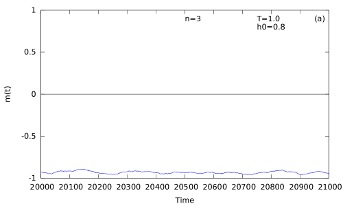
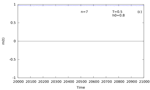
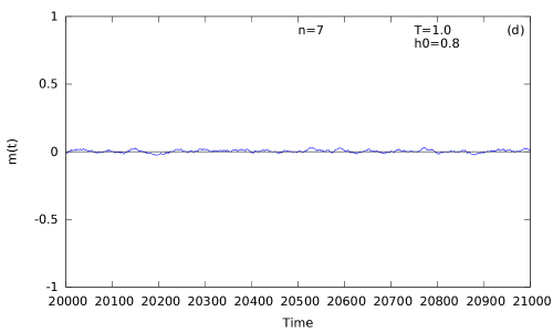
Figure 1: Variation of magnetisation with time at constant temperature ($T$) and field amplitude ($h_{0}$) for propagating wave. Fig.1a & fig.1b. represent 3-state spin whereas fig.1c. & fig.1d. represent 7-state spin. Frequency $f=0.01$.

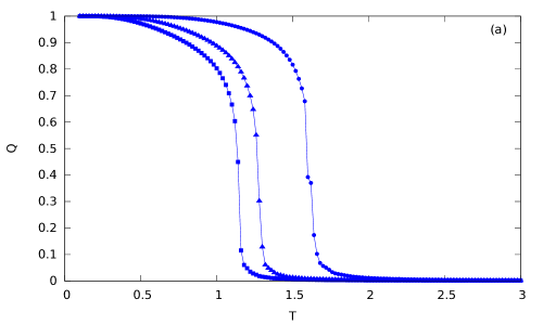
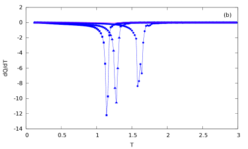
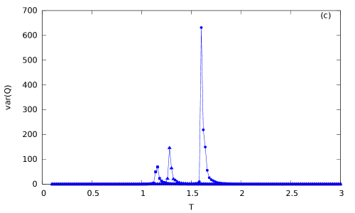
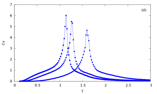
Figure 2: Temperature variation of (a) $Q$, (b) $\frac{dQ}{dT}$, (c) $V$, (d) $C_{v}$ for 3-state (circle), 5-state (uptriangle) and 7-state (square) spins for constant field amplitude ($h_{0}=0.2$) and frequency ($f=0.01$) of propagating wave.

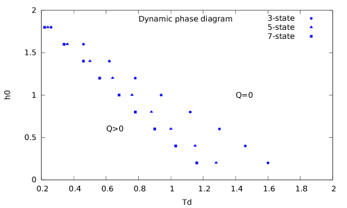
Figure 3: Phase diagram in $T_{d}$-$h_{0}$ plane for 3-state (circle), 5-state (uptriangle) and 7-state (square) spins for propagating wave.

To study the nonequilibrium behaviour of S-spin Ising ferromagnet in 2D we have taken a lattice of dimension ($100\times 100$). Propagating magnetic field waves having different values of field amplitude $h_{0}$ but fixed wavelength $(\lambda=25\ lattice\ units(lu))$ and frequency $(f=0.01\ MCSS^{-1})$ are allowed to pass through the system. The dynamical quantities at any temperature $T$ is calculated when the system has achieved steady state. For this we have kept the system at constant temperature $T$ for a sufficient long time ($100000\ MCSS$) i.e. through $1000$ complete cycles of magnetic oscillations while discarding initial (or transient) $500$ cycles and taking average over the remaining $50000\ MCSS$. We have identified a phase transition between high temperature symmetric phase and low temperature symmetry-broken phase. The order parameter for the phase transition is defined as the average magnetisation of each spin over a complete cycle of magnetic field oscillation, i.e. $Q=f\times\oint M(t)dt$, where $M(t)$ is the instantaneous magnetisation per spin state at time $t$. At very high temperature the order parameter has a low value which means that the spins are symmetrically distributed over all of their S states. At high temperature thermal energy of spins exceeds their mutual interaction energy and hence in varying magnetic field these spins flips more easily along the direction of field oscillation depending upon the strength of the magnetic field. As a result this phase propagates coherently alongwith the propagating wave. This propagation of spins have no relation with the conventional spin waves in ferromagnets. This phase may also be called as propagating phase. When the system is cooled down and the magnetic energy alongwith the thermal energy becomes insufficient to overcome the mutual interaction strength between any pair of spins this symmetric distribution of spin states breaks and the absolute value of magnetisation begins to grow as the temperature falls below the transition temperature. Thus the value of the order parameter becomes high. The variations of the instantaneous magnetisation per spin state, measured as $M(t)={{1}\over{L^{2}}}\sum_{i}S_{i}^{z}(x,y,t)$, with time in symmetric phase and symmetry-broken phase are shown in figs.1 for $3$-state and $7$-state spins respectively. In symmetric phase magnetisation varies around zero value resulting in very low average whereas it varies around a nonzero value in symmetry-broken phase. Figs.2 show the variation of different dynamical quantities at steady state; such as: order parameter $(Q)$, time derivative of the order parameter $\frac{dQ}{dT}$, variance of the order parameter $(V=L^{2}(\langle Q^{2}\rangle-\langle Q\rangle^{2}))$, and the dynamic heat capacity $(C_{v}=\frac{dE}{dT})$ for $3$-state, $5$-state and $7$-state spins respectively. Order parameter takes on nonzero value as the system cools and becomes unity below certain transition temperature defining the dynamic phase transition. The transition is detected by the sharp variations of $\frac{dQ}{dT}$, $V$ and $C_{v}$ at the transtion temperature $(T_{d})$. It is observed that the transition temperature decreases and approaches a minimum value as the number of spin states increases. Fig.3 shows the dynamic phase diagrams $(T_{d}\ vs\ h_{0})$ for 3-state, 5-state and 7-state spins respectively which shrinks inwards for greater number of spin states $S$. These also manifest that the transition occurs at lower temperature ($T_{d}$) for higher values of field amplitude ($h_{0}$) as we usually observe in other studies with 2-state Ising spins. Here, it may be noted that the typical size of the errorbar of the data in Fig-2 is around 0.03. From the peak (or dip) positions of various quantities the transition temperature was determined. Here the maximum possible error in estimating the transition temperature will be 0.02 (this is the value of $\Delta T$ by which the temperature of the system is reduced). So, the data shown in the phase diagram (in Fig-3) involves the error of size 0.02 in the estimation of transition temperature.

3.2. Standing field wave:

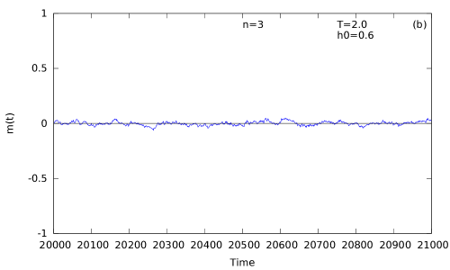
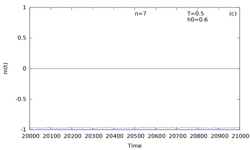
Figure 4: Variation of magnetisation with time at constant temperature ($T$) and field amplitude ($h_{0}$) for standing wave. Fig.4a & fig.4b. represent 3-state spin whereas fig.4c. & fig.4d. represent 7-state spin. Frequency $f=0.01$.

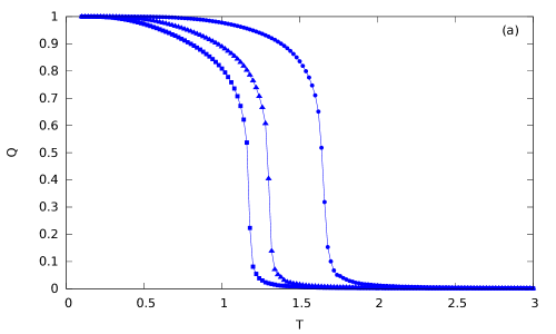
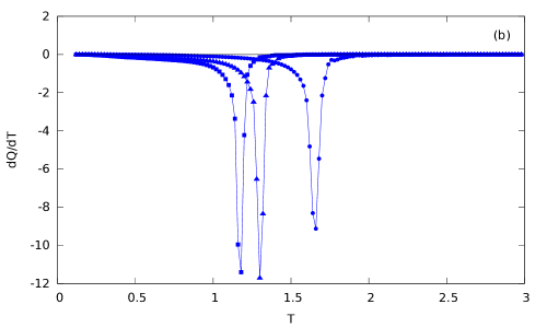
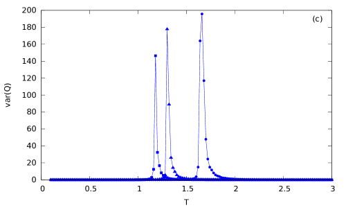
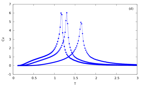
Figure 5: Temperature variation of (a) $Q$, (b) $\frac{dQ}{dT}$, (c) $V$, (d) $C_{v}$ for 3-state (circle), 5-state (uptriangle) and 7-state (square) spins for constant field amplitude ($h_{0}=0.2$) and frequency ($f=0.01$) of standing wave.

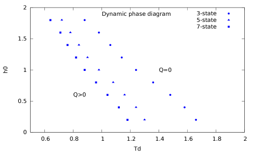
Figure 6: Phase diagram in $T_{d}$-$h_{0}$ plane for 3-state (circle), 5-state (uptriangle) and 7-state (square) spins for standing wave.

The dynamic phase transition is also observed in Ising ferromagnet having S number of spin states driven by standing magnetic wave. Here also the lattice size is $100\times 100$. In our study we have chosen fixed value for wavelength of the wave which is $\lambda=24.5\ lu$ so that there are exactly 8 loops of magnetic oscillation in a lattice. The frequency of magnetic oscillation is taken as $(f=0.01\ MCSS^{-1})$. Steady state dynamical behaviour is observed by keeping the system in constant temperature for a sufficently long time $200000\ MCSS$ i.e. for through $2000$ complete oscillations of magnetic field. Various dynamical quantities are calculated after discarding initial $1000$ cycles of oscillations and then taking average over the remaining $100000\ MCSS$. At steady state we have observed a dynamical phase transition between high temperature symmetric phase and low temperature symmetry-broken phase similar to that with propagating wave. The order parameter for the transition is also defined in a way similar to that of the propagating wave. At sufficiently high temperature all the S states of spin have equal probability and hence the average magnetisation per spin $M(t)$ at any time $t$ is nearly zero, which is shown in fig.4b & fig.4d for 3-state and 7-state spins respectively, whereas at low temperature thermal energy of spins are much less and the probability of spin flip is mainly magnetic field driven. If the magnetic field amplitude becomes low the mutual interaction energy between any pair of spins does not allow them to respond to the variations of magnetic field coherently and hence the value of magnetisation per spin at any time $t$ takes nonzero value as shown by the fig.4a. & fig.4c. respectively for 3-state and 7-state spins. Unlike the situation in propagating magnetic field wave, in standing magnetic wave there is a local variation of field amplitude; zero at the nodes and maximum at the antinodes. So at nodes of the standing wave the dynamics of the spin states are always thermally driven but at antinodes the value of field amplitude may have the effect on spin flip at relatively lower but above the transition temperature. Above the transition temperature alternate bands of spins ($s^{z}=+1\ or\ -1$) forming standing wave is observed. This wave is not the usual spin wave in ferromagnets. Near the boundaries of the standing wave bands there are almost equal population of all S-states of spin. Below the transition temperature field energy as well as thermal energy is insufficient to alter any spin state and all the ferromagnetic spins orient themselves in a particular direction giving rise to symmetry-broken or spin-frozen phase with nonzero magnetisation per spin. Thus the order parameter varies continuously from zero at high temperature to unity below the transition temperature as shown in fig.5a. for 3-state, 5-state and 7-state spins respectively. The transition is detected by observing the sharp variation of $\frac{dQ}{dT}$, $V$ and $C_{v}$ with temperature near the dynamic transition temperature $T_{d}$. These variations are shown in fig.5b., fig.5c. and fig.5d. respectively. All of these variations show that the transition temperature decreases and approaches a minimum value as the number of spin states increases. We have also drawn three comprehensive phase boundaries for 3-state, 5-state and 7-state spins in $T_{d}$-$h_{0}$ plane (fig.6.). It is observed here also that the phase boundary shrinks inwards for greater number of spin states. The phase boundaries also show that the transition temperature decreases as the magnetic field amplitude increases similar to previous results obtained with 2-state Ising spins. Here, it may be noted that the typical size of the errorbar of the data in Fig-5 is around 0.03. From the peak (or dip) positions of various quantities the transition temperature was determined. Here the maximum possible error in estimating the transition temperature will be 0.02 (this is the value of $\Delta T$ by which the temperature of the system is reduced). So, the data shown in the phase diagram (in Fig-6) involves the error of size 0.02 in the estimation of transition temperature.

3.3. Uniformly Oscillating field:

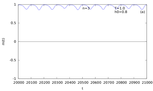
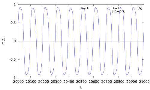
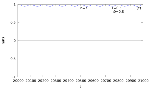
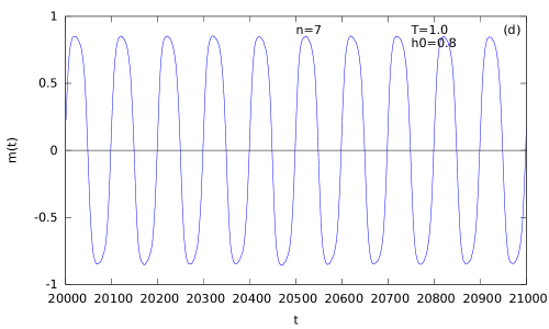
Figure 7: Variation of magnetisation with time at constant temperature ($T$) and field amplitude ($h_{0}$) for uniformly varying field. Fig.7a & fig.7b. represent 3-state spin whereas fig.7c. & fig.7d. represent 7-state spin. Frequency $f=0.01$.

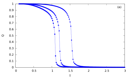
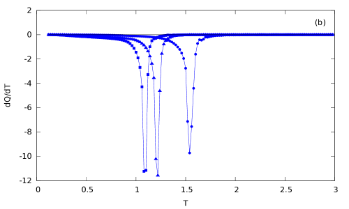
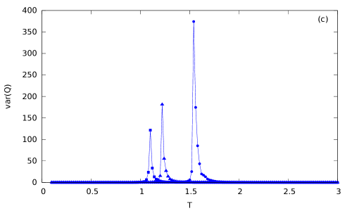
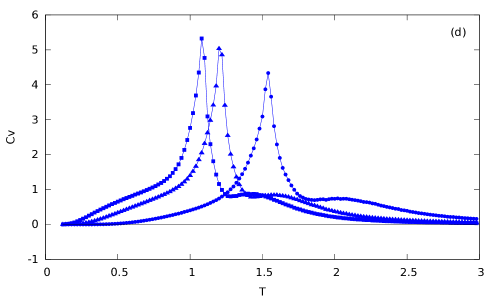
Figure 8: Temperature variation of (a) $Q$, (b) $\frac{dQ}{dT}$, (c) $V$, (d) $C_{v}$ for 3-state (circle), 5-state (uptriangle) and 7-state (square) spins for constant field amplitude ($h_{0}=0.3$) and frequency ($f=0.01$) of uniformly varying field.

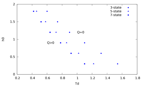
Figure 9: Phase diagram in $T_{d}$-$h_{0}$ plane for 3-state (circle), 5-state (uptriangle) and 7-state (square) spins for uniformly varying field.

We have also checked the nonequilibrium phase transition in S-state Ising ferrromagnets under uniformly oscillating magnetic field, where there is no spatial variation of the magnetic field throughout the Ising spin lattice. We kept the size of the lattice and the frequency of magnetic field oscillation similar to the above mentioned studies with propagating and standing magnetic wave. Steady state behaviour is studied as previously mentioned. It is observed that the system undergoes phase transition from high temperature symmetric phase to low temperature symmetry-broken phase depending on the values of the magnetic field amplitude $h_{0}$ and the number of spin states $S$. At sufficiently high temperature spins are uniformly distributed over all of its states which is considered as the initial state of the spin system. As the temperature is cooled this uniform distribution over all the states is no longer observed, rather spins orient themselves along the direction of the externally applied magnetic field and average magnetisation per spin $(M(t))$ follows the magnetic oscillation. The value of order parameter is zero as a result. This is shown in fig.7b. and fig.7d. for 3-state and 7-state spins respectively. At temperature below the transition temperature the probability of spin flip is much low and the spins freeze in a fixed direction parallel to the magnetic oscillation and $M(t)$ takes nonzero value as shown in the fig.7a. and fig7c. respectively. The value of order parameter hence also becomes nonzero. The variations of $Q$, $\frac{dQ}{dT}$, $V$ and $C_{v}$ with temperature $T$ are shown in the fig.8a., fig.8b., fig.8c. and fig.8d. respectively. The variations observed in these figures show that the transition temperature decreases and approaches a minimum value as the number of spin states increases. We have also drawn comprehensive phase boundaries for 3-state, 5-state and 7-state spins in $T_{d}$-$h_{0}$ plane (fig.9.) which shrink inwards for greater number of spin states $S$. These phase boundaries also reveals that the transition temperature decreases as the field amplitude increases. Here, it may be noted that the typical size of the errorbar of the data in Fig-8 is around 0.03. From the peak (or dip) positions of various quantities the transition temperature was determined. Here the maximum possible error in estimating the transition temperature will be 0.02 (this is the value of $\Delta T$ by which the temperature of the system is reduced). So, the data shown in the phase diagram (in Fig-9) involves the error of size 0.02 in the estimation of transition temperature.

4. Summary:

The dynamics of $S$-state Ising ferromagnet in the presence of propagating magnetic wave, standing magnetic wave and uniformly oscillating magnetic field has been studied here using Monte Carlo simulation with parallel updating rule for the spin states. Two distinct dynamical phases namely: symmetric phase and symmetry-broken phase are observed depending on the values of temperature, strength of the magnetic field and the number of states of the Ising spins for all kinds of magnetic excitations. For a fixed field amplitude the dynamic transition temperature decreases as the number of spin states increases. Transitions occur also at lower temperature for higher magnetic field amplitudes for a fixed number of spin states. The symmetric phase propagates coherently with the propagating magnetic wave whereas in case of standing magnetic wave alternate bands of spins oscillate out of phase forming standing waves of spin bands in symmetric phase. For uniformly oscillating field the spins oscillates coherently with the magnetic field. Below transition temperature the spins orient in some fixed direction (either up or down) and are not affected by the magnetic fields, yielding the maximum for the absolute value of magnetisation. The transitions are detected by observing the variations of $Q$, $\frac{dQ}{dT}$, $V$ and $C_{v}$ with $T$. Transition temperatures, found from the peaks in the $V$-$T$ or $C_{v}$-$T$ curves are employed to draw the phase boundaries.

Qualitative nature of the nonequilibrium phase transition driven by different magnetic excitations are more or less same in case of multiple state Ising spins. The transition temperature decreases towards a limiting value (in the limit of very large number of states) with greater number of spin states.

The question naturally arises here, what is the reason of considering different types of external driving magnetic field. Although the qualitative nature of the phase boundary is same for all different types of magnetic fields, the morphological structures of the dynamical spin configurations are different for different kinds of magnetic field. These are shown explicitly in the figures. For propagating magnetic field Fig-10 shows the coherent propagation of spin bands. The variations of spin configuration with temperature , field amplitude and the values of spin S , are shown in Fig-11. As a contrast, the coherent spin propagation is absent in the case of standing magnetic wave. In this case, the change in values (of the spins) of the alternate bands is observed here. This is shown in Fig-12. Here also, the variations of spin configuration with temperature, field amplitude and values of spin S, are shown in Fig-13. The uniform (over the space) and time dependent (sinusoidal) magnetic field does not have any spatial variation at any instant of time. So, one should not expect any dynamical pattern in the spin configuration. This is shown in Fig-14. The variations of spin configuration (without any significant pattern) with temperature , field amplitude and values of spin S, are shown in Fig-15.

The present study, though looks pedagogical, has a motivation with experimental background. Recently, the site diluted Blume-Capel model was studied[34] by meanfield renormalization group analysis with good agreement of the experimental phase diagram of Fe-Al alloy. In our case, studied here, this can be generalised for S=1 Ising ferromagnet. This coherent propagation of spin bands can be experimentally studied by time resolved magneto optic Kerr (TRMOKE) effect. We believe, that this has a significant role in the field of spintronics and magmonincs[35]. The magnetic behaviours of core-shell magnetic nanoparticles has an important role in the magnetism research as well as in the technology. The properties of magnetism have been studied[36] in bimagnetic ($FePt/MFe_{2}O_{4}(M=Fe,Co))$ core-shel nanoparticles. The nonequilibrium phase transition has been studied [37] by Monte Carlo simulation in spherical core-shell (s=3/2 core and s=1 shell) under time dependent (uniform over space) magnetic field. We propose to study the dynamic responses of core-shell magnetic nanoparticles in the presence of magnetic field having spatio temporal variation in the form of propagating and standing magnetic wave.

V. References:

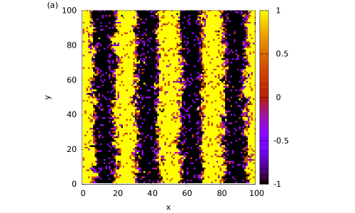
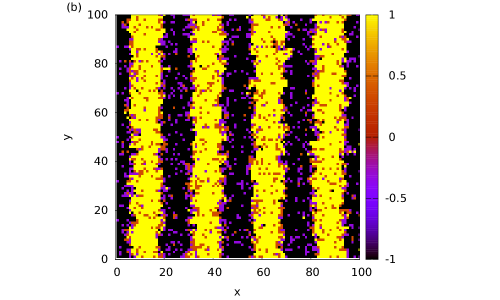
Figure 10: Coherent propagation of spin-wave is shown at two different times for propagating magnetic wave: (a) at $t=4018$ and (b) at $t=4067$. Here $n=4$, $h_{0}=1.0$ & $T=1.2$.

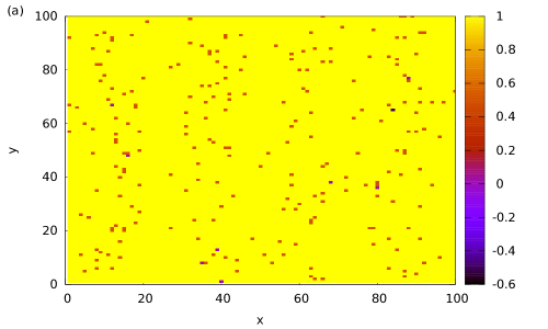
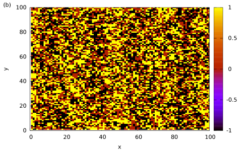
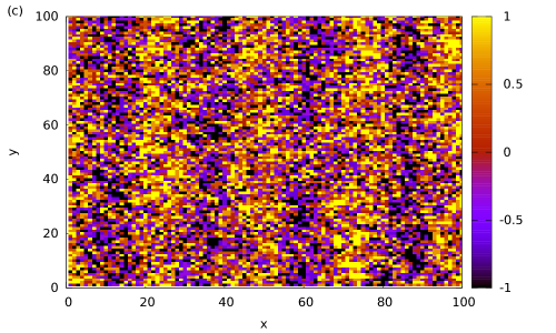
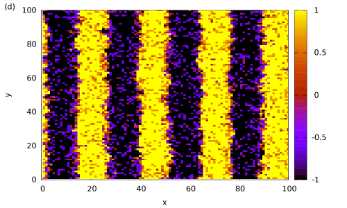
Figure 11: Lattice morphology (value of $S^{z}(x,y,t)$) at time $t=4000$ for different values of $n$, $h_{0}$ and $T$ for propagating magnetic wave: (a) $n=5$, $h_{0}=0.8$ & $T=0.5$, (b) $n=3$, $h_{0}=0.2$ & $T=2.8$, (c) $n=7$, $h_{0}=0.3$ & $T=1.8$ and (d) $n=7$, $h_{0}=1.2$ & $T=0.8$.

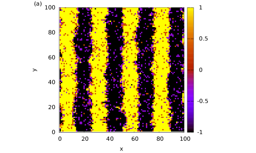
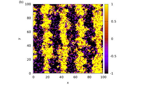
Figure 12: Morphologies of standing wave dynamical modes (non-propagating) for standing magnetic wave are shown at two different times: (a) at $t=4040$ and (b) at $t=4067$. Here $n=4$, $h_{0}=1.2$ & $T=1.2$.

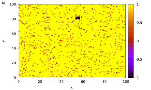
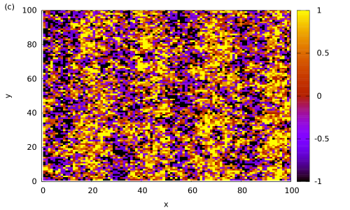
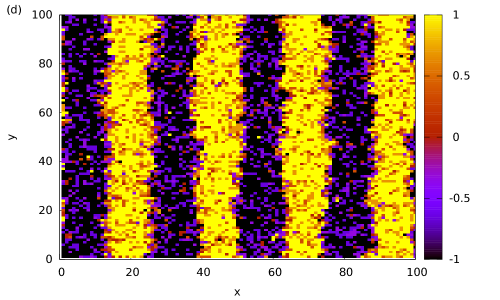
Figure 13: Lattice morphology (value of $S^{z}(x,y,t)$) at time $t=4000$ for different values of $n$, $h_{0}$ and $T$ for standing magnetic wave: (a) $n=5$, $h_{0}=0.8$ & $T=0.8$, (b) $n=3$, $h_{0}=0.2$ & $T=2.2$, (c) $n=7$, $h_{0}=0.3$ & $T=1.5$, & (d) $n=7$, $h_{0}=1.2$ & $T=1.0$.

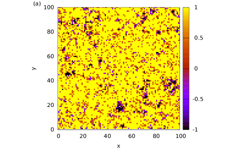
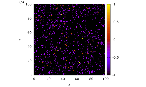
Figure 14: Oscillation of spins shown at different times ($t=4000$ & $t=4067$) in symmetric phase for uniformly oscillating magnetic field. Here $n=4$, $h_{0}=1.2$ & $T=1.2$.

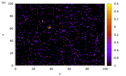
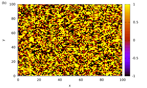
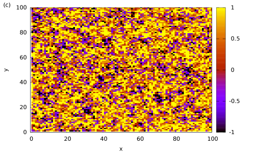
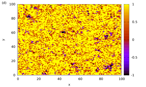
Figure 15: Lattice morphology (value of $S^{z}(x,y,t)$) for different values of $n$, $h_{0}$ and $T$ for uniformly oscillating magnetic field: (a) $n=5$, $h_{0}=0.8$ & $T=0.8$ at time $t=3950$ and (b) $n=3$, $h_{0}=0.2$ & $T=2.9$, (c) $n=7$, $h_{0}=0.3$ & $T=1.5$, & (d) $n=7$, $h_{0}=1.2$ & $T=1.0$ at time $t=4000$.

References

- [1] B. K. Chakrabarti and M. Acharyya, Rev. Mod. Phys. 71 (1999) 847
- [2] M. Acharyya, Int. J. Mod. Phys. C16 (2005) 1631
- [3] M. Acharyya, Phys. Rev. E 56, 2407 (1997).
- [4] M. Acharyya, Physica A 235, 469 (1997).
- [5] S. W. Sides, P. A. Rikvold, M. A. Novotny, Phys. Rev. Lett. 81, 834 (1998).
- [6] M. Acharyya, Phys. Rev. E 59, 218 (1999).
- [7] G. Korniss, P. A. Rikvold, M. A. Novotny, Phys. Rev. E 66, 056127 (2002)
- [8] M. Acharyya, Phys. Rev. E 58, 179 (1998).
- [9] M. Acharyya, Int. J. Mod. Phys. C 14, 49 (2003).
- [10] H. Jung, M. J. Grimson, C. K. Hall, Phys. Rev. B 67, 094411 (2003).
- [11] H. Jung, M. J. Grimson, C. K. Hall, Phys. Rev. E 68, 046115 (2003).
- [12] M. Keskin, O. Canko, B. Deviren, Phys. Rev. E 74, 011110 (2006).
- [13] U. Temizer, E. Kantar, M. Keskin, O. Canko, J. Magn. Magn. Mater, 320, 1787 (2008).
- [14] M. Ertas, B. Deviren and M. Keskin, Phys. Rev. E, 86 (2012) 051110
- [15] U. Temizer, J. Magn. Magn. Mater, 372 (2014) 47
- [16] E. Vatansever, A. Akinci and H. Polat, J. Magn. Magn. Mater, 389 (2015) 40
- [17] M. Ertas and M. Keskin, Physica A, 437 (2015) 430
- [18] X. Shi, L. Wang, J. Zhao, X. Xu, J. Magn. Magn. Mater, 410 (2016) 181
- [19] D. M. Saul, M. Wortis and D. Stauffer, Phys. Rev. B, 9 (1974) 4964
- [20] A. K. Jain and D. P. Landau, Phys. Rev. B, 22 (1980) 445
- [21] M. Deserno, Phys. Rev. E, 56 (1997) 5204
- [22] J. C. Xavier, F. C. Alcaraz, D. P. Lara, J. A. Plascak, Phys. Rev. E, 57 (1998) 11575
- [23] M. Ertas, M. Keskin and B. Deviren, J. Magn. Magn. Mater, 324 (2012) 1503
- [24] C. Yunus, B. Renklioglu, M. Keskin and A. N. Berker, Phys. Rev. E, 93 (2016) 062113
- [25] J. A. Plascak, J. G. Moreira, F. C. saBarreto, Phys. Lett. A, 173 (1993) 360
- [26] T. Fiig, B. M. Gorman, P. A. Rikvold and M. A. Novotny, Phys. Rev. E, 50 (1994) 1930
- [27] F. Manzo and E. Olivieri, J. Stat. Phys, 104 (2001) 1029
- [28] M. Acharyya, J. Magn. Magn. Mater, 354 (2014) 349
- [29] M. Acharyya, J. Magn. Magn. Mater, 382 (2015) 206
- [30] M. Acharyya, Acta Physica Polonica B, 45 (2014) 1027
- [31] A. Halder and M. Acharyya, J. Magn. Magn. Mater, 420 (2016) 290
- [32] M. Acharyya and A. Halder, J. Magn. Magn. Mater, 426 (2017) 53
- [33] K. Binder and D. W. Heermann, Monte Carlo simulation in statistical physics, Springer series in solid state sciences, Springer, New-York, 1997
- [34] D. Das and J. A. Plascak, Phys. Lett. A, 375 (2011) 2089
- [35] S. Bader and S. S. P. Parkin, Annu. Rev. Condens. Matter Phys, 1 (2010) 71-88
- [36] H. Zeng, S. Sun, J. Li, Z. L. Wang and J. P. Liu, Applied Physics Letters, 85 (2004) 792
- [37] E. Vatansever and H. Polat, J. Magn. Magn. Mater, 343 (2013) 221