Gaussian Process Model Predictive Control of An Unmanned Quadrotor

Abstract

The mpc trajectory tracking problem of an unmanned quadrotor with input and output constraints is addressed. In this article, the dynamic models of the quadrotor are obtained purely from operational data in the form of probabilistic gp models. This is different from conventional models obtained through Newtonian analysis. A hierarchical control scheme is used to handle the trajectory tracking problem with the translational subsystem in the outer loop and the rotational subsystem in the inner loop. Constrained gp based mpc are formulated separately for both subsystems. The resulting mpc problems are typically nonlinear and non-convex. We derived a gp based local dynamical model that allows these optimization problems to be relaxed to convex ones which can be efficiently solved with a simple active-set algorithm. The performance of the proposed approach is compared with an existing unconstrained nmpc. Simulation results show that the two approaches exibit similar trajectory tracking performance. However, our approach has the advantage of incorporating constraints on the control inputs. In addition, our approach only requires $\displaystyle 20\%$ of the computational time for nmpc.

1 Introduction

The quadrotor helicopter (or quadrotor for short) is an aerial vehicle with vertical take-off and landing capabilities. It has received a lot of interests recently due to its simplicity, maneuverability, and payload capabilities A-Alexis-SwitchMPC-QuadrotorUAV-2011 ; A-Abdolhosseini-MPC-QuadrotorUAV-2013 . It has been used in various military and civilian tasks A-Metni-UAV-BridgeInspection-2007 ; IC-Doherty-UAV-HumanBodyDetection-2007 .

Trajectory tracking is one of the basic functions performed by a quadrotor in autonomous flight. Designing a control system to perform this function is challenging because the quadrotor’s dynamics are highly nonlinear and are subjected to random external disturbances. Several control approaches have previously been investigated with varying degrees of success. They include linear techniques such as pid and lqr control IP-Bouabdallah-PID/LQ-UAV-2004 , as well as nonlinear techniques such as sliding mode IP-Madani-SlidingModeAndBackStepping-UAV-2007 and backstepping control IP-Huang-AdaptiveTrackingUsingBackstepping-UAV-2010 . More recently, due to the conceptual simplicity, mpc techniques have been used in A-Raffo-HinfinityControl-UAV-2010 ; A-Alexis-SwitchMPC-QuadrotorUAV-2011 based on the linearised model and in A-Abdolhosseini-MPC-QuadrotorUAV-2013 based on the nonlinear model. Moreover, physical constraints on the system inputs and outputs, which is important for quadrotors, could easily be included as appropriate penalty terms in the cost function that is used to compute the optimal control.

The performance of mpc is highly dependent on how accurately the model describes the dynamics of the system being controlled. Conventionally, dynamical models are derived from first principles through Newton-Euler A-Zuo-QuadrotorTrackingControl-2010 or Euler-Lagrange based formalisms IP-Bouabdallah-PID/LQ-UAV-2004 . Alternatively, empirical input-output data could be collected from a real, working quadrotor. These data could then be used to construct a fm IP-Han-UAVfuzzymodelcontrol-2014 or an ann model IP-Voos-offlineNNbasedUAVcontrol-2007 ; A-Dierks-NNbasedUAVcontrol-2010 . This data-driven approach has the advantage that unknown dynamics that are not considered by Newtonian analysis could be captured by the empirical observations. However, it is difficult to evaluate the quality of these fm and ann models. gp modelling is an alternative data-driven technique based on Bayesian theory. Compared to ann and fm, a major advantage is that the quality of obtained gp model can be directly evaluated by gp variances which are naturally computed during the modelling and prediction processes. gp based technique has recently been used to learn the flight model of uav IP-Hemakumara-IndentificationUAVusingDGP-2011 ; IP-Hemakumara-IndentificationUAVusingDGP-2013 and quadrotors IP-Berkenkamp-RboustLBNMPC-2014 ; IP-GPMPC4Quad-Gang-2016b .

The cost functions used in early gp based mpc problems are deterministic even though the gp models are probabilistic IP-Kocijan-MPC-2003 ; IP-Kocijan-MPC-GP-2004 ; A-Likar-MPC-2007 ; IP-Grancharova-ApproxExplicitNMPC-2007 . This issue has been addressed recently in A-Klenske-GPMPC4Periodic-2015 ; IP-GPMPC4LTV-Gang-2016a ; IP-GPMPC4Quad-Gang-2016b where the expectation of the cost function is used instead, as proposed in A-Mesbah-SMPC-2016 . However, these works did not take into consideration any constraint on system inputs and outputs. In addition, a computationally efficient method is required to solve the resulting gp based mpc optimization problem which is usually nonlinear and non-convex.

In this article, a hierarchical control scheme is applied to the trajectory tracking problem of a quadrotor, where a translational subsystem forms the outer loop and a rotational subsystem is in the inner loop A-Raffo-HinfinityControl-UAV-2010 ; A-Alexis-SwitchMPC-QuadrotorUAV-2011 . Each subsystem is independently modelled by a gp model. We propose a gp based mpc control scheme, referred to as GPMPC, solve the resulting two mpc tracking problems. It tackles the issues mentioned above regarding the objective function and computational efficiency. The performance of GPMPC is evaluated by simulations on two non-trivial trajectories.

2 Quadrotor System Modelling Using GP

The quadrotor can be viewed as a 6 dof rigid body with generalized coordinates $\displaystyle\mathbf{q}=[x,y,z,\phi,\theta,\psi]^{T}\in\mathbb{R}^{6}$, where $\displaystyle x,y,z$ denotes the quadrotor’s positions w.r.t. earth-fixed frame (E-frame) and $\displaystyle\phi,\theta,\psi$ represents quadrotor’s attitudes w.r.t. body-fixed frame (B-Frame). Motion is controlled by a main thrust $\displaystyle U_{1}$ and three torques $\displaystyle U_{2}$, $\displaystyle U_{3}$ and $\displaystyle U_{4}$. Thus it is an underactuated system. Furthermore, the dynamical model of the quadrotor is defined by the state-space function $\displaystyle\ddot{\mathbf{q}}=f_{\mathbf{q}}(\mathbf{q},\dot{\mathbf{q}},U_{1},U_{2},U_{3},U_{4})$ which is usually nonlinear A-Raffo-HinfinityControl-UAV-2010 . In order to simplify the control of the quadrotor, the system is typically decomposed into two subsystems – a translational subsystem and a rotational subsystem. Let the system state of the translational subsystem be $\displaystyle\mathbf{x}^{\xi}=[x,\dot{x},y,\dot{y},z,\dot{z}]^{T}\in\mathbb{R}^{6}$ and its control be $\displaystyle\mathbf{u}^{\xi}=[U_{1},u_{x},u_{y}]^{T}\in\mathbb{R}^{3}$. The dynamics of this subsystem can be described by A-Raffo-HinfinityControl-UAV-2010

$$\dot{\mathbf{x}}^{\xi}=f_{\xi}\left(\mathbf{x}^{\xi},\mathbf{u}^{\xi}\right)+\bm{\epsilon}^{\xi}$$ (1)

where $\displaystyle f_{\xi}:\mathbb{R}^{6}\times\mathbb{R}^{3}\rightarrow\mathbb{R}^{6}$ is nonlinear and is usually corrupted by white noises $\displaystyle\bm{\epsilon}^{\xi}\in\mathbb{R}^{6}$. $\displaystyle u_{x}$ and $\displaystyle u_{y}$ are two intermediate controls to actuate the translational subsystem and are given by

$$u_{x} =\cos{\phi}\sin{\theta}\cos{\psi}+\sin{\phi}\sin{\psi}$$ (2)

$$u_{y} =\cos{\phi}\sin{\theta}\sin{\psi}-\sin{\phi}\cos{\psi}$$

Similarly, let $\displaystyle\mathbf{x}^{\eta}=[\phi,\dot{\phi},\theta,\dot{\theta},\psi,\dot{\psi}]^{T}\in\mathbb{R}^{6}$ and $\displaystyle\mathbf{u}^{\eta}=[U_{2},U_{3},U_{4}]^{T}\in\mathbb{R}^{3}$ be the state and control for the rotational subsystem. Its system equation is given by A-Raffo-HinfinityControl-UAV-2010

$$\dot{\mathbf{x}}^{\eta}=f_{\eta}\left(\mathbf{x}^{\eta},\mathbf{u}^{\eta}\right)+\bm{\epsilon}^{\eta}$$ (3)

where $\displaystyle f_{\eta}:\mathbb{R}^{6}\times\mathbb{R}^{3}\rightarrow\mathbb{R}^{6}$ is another nonlinear function and $\displaystyle\bm{\epsilon}^{\eta}\in\mathbb{R}^{6}$ represents the white noise.

2.1 GP Modelling

The system equations (1) and (3) of both subsystems can be expressed in the following general form in the discrete-time domain by

$$\mathbf{x}_{k+1}=f(\mathbf{x}_{k},\mathbf{u}_{k})+\mathbf{w}_{k}$$ (4)

where $\displaystyle\mathbf{x}_{k}\in\mathbb{R}^{n}$ denotes an $\displaystyle n$-dimensional state vector and $\displaystyle\mathbf{u}_{k}\in\mathbb{R}^{m}$ represents an $\displaystyle m$-dimensional input vector at the sampling time $\displaystyle k$. $\displaystyle f:\mathbb{R}^{n}\times\mathbb{R}^{m}\rightarrow\mathbb{R}^{n}$ is a discrete nonlinear function, and $\displaystyle\mathbf{w}_{k}\in~{}\mathbb{R}^{n}$ is Gaussian white noise. To learn such an unknown function $\displaystyle f(\cdot)$ using gp modelling techniques, a natural choice for the model inputs and outputs are the state-control tuple $\displaystyle\tilde{\mathbf{x}}_{k}=(\mathbf{x}_{k},\mathbf{u}_{k})\in\mathbb{R}^{n+m}$ and the next state $\displaystyle\mathbf{x}_{k+1}$ respectively. However, in practice, the difference $\displaystyle\Delta\mathbf{x}_{k}=\mathbf{x}_{k+1}-\mathbf{x}_{k}\in\mathbb{R}^{n}$ is usually smaller less than the values of $\displaystyle\mathbf{x}_{k}$. Thus it is more advantageous to use $\displaystyle\Delta\mathbf{x}_{k}$ as the model output instead PHD-Deisenroth-EfficientRLusingGP-2010 .

A gp model is completely specified by its mean and covariance function B-GPMLbook-2006 . Assuming that the mean of the model input $\displaystyle\tilde{\mathbf{x}}_{k}$ is zero, the squared exponential covariance is given by $\displaystyle\mathbf{K}(\tilde{\mathbf{x}}_{i},\tilde{\mathbf{x}}_{j})=\sigma_{s}^{2}\exp(-\frac{1}{2}(\tilde{\mathbf{x}}_{i}-\tilde{\mathbf{x}}_{j})^{T}\bm{\varLambda}(\tilde{\mathbf{x}}_{i}-\tilde{\mathbf{x}}_{j}))+\sigma_{n}^{2}$, where $\displaystyle i$ and $\displaystyle j$ denote two sampling time steps. The parameters $\displaystyle\sigma_{s}^{2},\sigma_{n}^{2}$ and the entries of matrix $\displaystyle\bm{\varLambda}\in\mathbb{R}^{(n+m)\times(n+m)}$ (usually is a diagonal matrix) are referred to as the hyperparameters $\displaystyle\bm{\theta}$ of a gp model. Given $\displaystyle D$ training inputs $\displaystyle\tilde{\mathbf{X}}=[\tilde{\mathbf{x}}_{1},\cdots,\tilde{\mathbf{x}}_{D}]\in\mathbb{R}^{(n+m)\times D}$ and their corresponding training targets $\displaystyle\mathbf{y}=[\Delta\mathbf{x}_{1},\cdots,\Delta\mathbf{x}_{D}]^{T}\in\mathbb{R}^{nD}$, the joint distribution between $\displaystyle\mathbf{y}$ and a test target $\displaystyle\Delta\mathbf{x}^{*}_{k}$ corresponding to the test input $\displaystyle\tilde{\mathbf{x}}_{k}^{*}$ at sampling time $\displaystyle k$ is assumed to follow a Gaussian distribution. That is

$$p\Bigg{(}\begin{array}[]{c}\mathbf{y}\\ \Delta\mathbf{x}^{*}_{k}\end{array}\Bigg{)}\sim\mathcal{N}\Bigg{(}{\color[rgb]{0,0,0}\mathbf{0}},\begin{array}[]{cc}\mathbf{K}(\tilde{\mathbf{X}},\tilde{\mathbf{X}})+\sigma_{n}\mathbf{I}&\mathbf{K}(\tilde{\mathbf{X}},\tilde{\mathbf{x}}^{*}_{k})\\ \mathbf{K}(\tilde{\mathbf{x}}^{*}_{k},\tilde{\mathbf{X}})&\mathbf{K}(\tilde{\mathbf{x}}^{*}_{k},\tilde{\mathbf{x}}^{*}_{k})\end{array}\Bigg{)}$$ (5)

where $\displaystyle\mathcal{N}(\cdot)$ denotes a multivariate Gaussian distribution and $\displaystyle\mathbf{0}\in\mathbb{R}^{nD}$ is a zero vector. In addition, the posterior distribution over the observations can be obtained by restricting the joint distribution to only contain those targets that agree with the observations. This is achieved by conditioning the joint distribution on the observations, and results in the predictive mean and variance function as follows B-GPMLbook-2006

$$\displaystyle m(\tilde{\mathbf{x}}^{*}_{k})=\textit{E}_{f}[\Delta\mathbf{x}^{*}_{k}] \displaystyle=\mathbf{K}(\tilde{\mathbf{x}}^{*}_{k},\tilde{\mathbf{X}})\mathbf{K}_{\sigma}^{-1}\mathbf{y}$$ (6a)

$$\displaystyle\sigma^{2}(\tilde{\mathbf{x}}^{*}_{k})=\textit{Var}_{f}[\Delta\mathbf{x}^{*}_{k}] \displaystyle=\mathbf{K}(\tilde{\mathbf{x}}^{*}_{k},\tilde{\mathbf{x}}^{*}_{k})$$ (6b)

$$\displaystyle-\mathbf{K}(\tilde{\mathbf{x}}^{*}_{k},\tilde{\mathbf{X}})\mathbf{K}_{\sigma}^{-1}\mathbf{K}(\tilde{\mathbf{X}},\tilde{\mathbf{x}}^{*}_{k})$$

where $\displaystyle\mathbf{K}_{\sigma}=\mathbf{K}(\tilde{\mathbf{X}},\tilde{\mathbf{X}})+\sigma_{n}\mathbf{I}$. The state at the next sampling time $\displaystyle k+1$ also follows a Gaussian distribution. That is

$$p(\mathbf{x}_{k+1})\sim\mathcal{N}(\bm{\mu}_{k+1},\bm{\Sigma}_{k+1})$$ (7)

where

$$\displaystyle\bm{\mu}_{k+1} \displaystyle=\mathbf{x}_{k}+m(\tilde{\mathbf{x}}^{*}_{k})$$ (8a)

$$\displaystyle\quad\bm{\Sigma}_{k+1} \displaystyle=\sigma^{2}(\tilde{\mathbf{x}}^{*}_{k})$$ (8b)

Typically, the hyperparameters of the gp model are learned by maximizing the log-likelihood function given by

$$\log p(\mathbf{y}|\tilde{\mathbf{X}},\bm{\theta})= -\frac{1}{2}\mathbf{y}^{T}\mathbf{K}_{\sigma}^{-1}\mathbf{y}-\frac{1}{2}\log\left|\mathbf{K}_{\sigma}^{-1}\right|$$ (9)

$$-\frac{D}{2}\log(2\pi)$$

This results in a nonlinear non-convex optimization problem that is traditionally solved by using cg or bfgs algorithms.

2.2 Uncertainty propagation

With the gp model obtained, one-step-ahead predictions can be made by using (6) and (8). When multiple-step predictions are required, the conventional way is to iteratively perform multiple one-step-ahead predictions using the estimated mean values. However, this process does not take into account the uncertainties introduced by each successive prediction. This issue has been shown to be important in time-series predictions IP-Girard-MultiStepTimeSeriesForecasting-2003 .

The uncertainty propagation problem can be dealt with by assuming that the joint distribution of the training inputs is uncertain and follows a Gaussian distribution. That is,

$$p(\tilde{\mathbf{x}}_{k})=p\big{(}\mathbf{x}_{k},\mathbf{u}_{k}\big{)}\sim\mathcal{N}(\tilde{\bm{\mu}}_{k},\tilde{\bm{\Sigma}}_{k})$$ (10)

with mean and variance given by

$$\displaystyle\tilde{\bm{\mu}}_{k} \displaystyle=\left[\bm{\mu}_{k},\textit{E}\left[\mathbf{u}_{k}\right]\right]^{T}$$ (11a)

$$\displaystyle\tilde{\bm{\Sigma}}_{k} \displaystyle=\left[\begin{array}[]{cc}\bm{\Sigma}_{k}&\textit{Cov}\left[\mathbf{x}_{k},\mathbf{u}_{k}\right]\\ \textit{Cov}\left[\mathbf{u}_{k},\mathbf{x}_{k}\right]&\textit{Var}\left[\mathbf{u}_{k}\right]\end{array}\right]$$ (11d)

where $\displaystyle\textit{Cov}\left[\mathbf{x}_{k},\mathbf{u}_{k}\right]=\textit{E}\left[\mathbf{x}_{k}\mathbf{u}_{k}\right]-\bm{\mu}_{k}\textit{E}\left[\mathbf{u}_{k}\right]$. Here, $\displaystyle\textit{E}\left[\mathbf{u}_{k}\right]$ and $\displaystyle\textit{Var}\left[\mathbf{u}_{k}\right]$ are the mean and variance of the system controls.

The exact predictive distribution of the training target could then be obtained by integrating over the training input distribution:

$$p(\Delta\mathbf{x}^{*}_{k})=\int p(f(\tilde{\mathbf{x}}^{*}_{k})|\tilde{\mathbf{x}}^{*}_{k})p(\tilde{\mathbf{x}}^{*}_{k})d\tilde{\mathbf{x}}^{*}_{k}$$ (12)

However, this integral is analytically intractable. Numerical solutions can be obtained using Monte-Carlo simulation techniques. In IP-Candela-GPUncertainPropagation-2003 , a moment-matching based approach is proposed to obtain an analytical Gaussian approximation. The mean and variance at an uncertain input can be obtained through the laws of iterated expectations and conditional variances respectively PHD-Deisenroth-EfficientRLusingGP-2010 . They are given by

$$\displaystyle m(\tilde{\mathbf{x}}^{*}_{k}) \displaystyle=\textit{E}_{\tilde{\mathbf{x}}^{*}_{k}}\Big{[}\textit{E}_{f}\big{[}\Delta\mathbf{x}^{*}_{k}\big{]}\Big{]}$$ (13a)

$$\displaystyle\sigma^{2}(\tilde{\mathbf{x}}^{*}_{k}) \displaystyle=\textit{E}_{\tilde{\mathbf{x}}^{*}_{k}}\Big{[}\textit{Var}_{f}\big{[}\Delta\mathbf{x}^{*}_{k}\big{]}\Big{]}+\textit{Var}_{\tilde{\mathbf{x}}^{*}_{k}}\Big{[}\textit{E}_{f}\big{[}\Delta\mathbf{x}^{*}_{k}\big{]}\Big{]}$$ (13b)

Equation (8) then becomes

$$\displaystyle\bm{\mu}_{k+1}= \displaystyle\bm{\mu}_{k}+m(\tilde{\mathbf{x}}^{*}_{k})$$ (14a)

$$\displaystyle\bm{\Sigma}_{k+1}= \displaystyle\bm{\Sigma}_{k}+\sigma^{2}(\tilde{\mathbf{x}}^{*}_{k})$$ (14b)

$$\displaystyle+\textit{Cov}\big{[}\mathbf{x}_{k},\Delta\mathbf{x}_{k}\big{]}+\textit{Cov}\big{[}\Delta\mathbf{x}_{k},\mathbf{x}_{k}\big{]}$$

The computational complexity of gp inference using (13) is $\displaystyle\mathcal{O}(D^{2}n^{2}(n+m))$ which is quite high. Hence, gp is normally only suitable for problems with limited dimensions (under 12 as suggested by most publications) and limited size of training data. For problems with higher dimensions, sparse gp approaches A-Sparse-Appro-2005 are often used.

3 Control Problem Formulation

Figure 1: The Overall Control Scheme for Quadrotor

3.1 MPC Problem for Subsystems

With the quadrotor system decomposed into two subsystems, a hierarchical structure as shown in Figure 1 can be used for the controller A-Raffo-HinfinityControl-UAV-2010 ; A-Alexis-SwitchMPC-QuadrotorUAV-2011 . In the outer loop, the translational subsystem is controlled to follow a sequence of desired positions $\displaystyle[x_{d},y_{d},z_{d}]^{T}$. The optimal control $\displaystyle U_{1}$ and two intermediate controls $\displaystyle u_{x}$ and $\displaystyle u_{y}$ are obtained by minimizing the tracking errors. With $\displaystyle\psi_{d}=0$, the desired attitudes $\displaystyle\theta_{d}$ and $\displaystyle\phi_{d}$ can be obtained using (2). Then, the rotational subsystem’s attitudes $\displaystyle[\phi,\theta,\psi]^{T}$ are tuned to achieve the given target values in the inner loop. By minimizing attitude errors, the optimal controls $\displaystyle U_{2}$, $\displaystyle U_{3}$ and $\displaystyle U_{4}$ can be obtained. Finally, the optimal control inputs $\displaystyle U_{1}$, $\displaystyle U_{2}$, $\displaystyle U_{3}$ and $\displaystyle U_{4}$ are applied to the quadrotor.

For a horizon of $\displaystyle H\geq 1$, the discrete mpc trajectory tracking problem in the outer loop is given by

$$\displaystyle\min_{\mathbf{u}^{\xi}(\cdot)} \displaystyle\sum_{i=1}^{H}\bigg{\{}\left\|\mathbf{x}^{\xi}_{k+i}-\mathbf{r}^{\xi}_{k+i}\right\|_{\mathbf{Q}^{\xi}}^{2}+\left\|\mathbf{u}^{\xi}_{k+i-1}\right\|_{\mathbf{R}^{\xi}}^{2}\bigg{\}}$$ (15a)

s.t. $$\displaystyle\mathbf{x}^{\xi}_{k+i+1}=f_{1}(\mathbf{x}^{\xi}_{k+i},\mathbf{u}^{\xi}_{k+i-1})$$ (15b)

$$\displaystyle\mathbf{x}^{\xi}_{\text{min}}\leq\mathbf{x}^{\xi}_{k+i}\leq\mathbf{x}^{\xi}_{\text{max}}$$ (15c)

$$\displaystyle\mathbf{u}^{\xi}_{\text{min}}\leq\mathbf{u}^{\xi}_{k+i-1}\leq\mathbf{u}^{\xi}_{\text{max}}$$ (15d)

where the $\displaystyle f_{1}(\cdot)$ represents the gp model of the translational subsystem. $\displaystyle\big{\|}\cdot\big{\|}_{\mathbf{Q}^{\xi}}$ and $\displaystyle\big{\|}\cdot\big{\|}_{\mathbf{R}^{\xi}}$ denote the two $\displaystyle 2$-norms weighted by positive definite matrices $\displaystyle\mathbf{Q}^{\xi}$ and $\displaystyle\mathbf{R}^{\xi}$ respectively. $\displaystyle\mathbf{x}^{\xi}_{k+i}$ and $\displaystyle\mathbf{u}^{\xi}_{k+i-1}$ are the system states and control inputs, and $\displaystyle\mathbf{r}^{\xi}_{k+i}=[x_{d,k+i},y_{d,k+i},z_{d,k+i}]^{T}$ denotes the desired positions at time $\displaystyle k+i$. In addition, $\displaystyle\mathbf{x}^{\xi}_{\text{max}}\geq\mathbf{x}^{\xi}_{\text{min}}$ and $\displaystyle\mathbf{u}^{\xi}_{\text{max}}\geq\mathbf{u}^{\xi}_{\text{max}}$ are the upper and lower bounds of the system states and control inputs respectively.

In the same way, for the inner loop, the discrete mpc optimization problem is given by

$$\displaystyle\min_{\mathbf{u}^{\eta}(\cdot)} \displaystyle\sum_{i=1}^{H}\bigg{\{}\left\|\mathbf{x}^{\eta}_{k+i}-\mathbf{r}^{\eta}_{k+i}\right\|_{\mathbf{Q}^{\eta}}^{2}+\left\|\mathbf{u}^{\eta}_{k+i-1}\right\|_{\mathbf{R}^{\eta}}^{2}\bigg{\}}$$ (16a)

s.t. $$\displaystyle\mathbf{x}^{\eta}_{k+i+1}=f_{2}(\mathbf{x}^{\eta}_{k+i},\mathbf{u}^{\eta}_{k+i-1})$$ (16b)

$$\displaystyle\mathbf{x}^{\eta}_{\text{min}}\leq\mathbf{x}^{\eta}_{k+i}\leq\mathbf{x}^{\eta}_{\text{max}}$$ (16c)

$$\displaystyle\mathbf{u}^{\eta}_{\text{min}}\leq\mathbf{u}^{\eta}_{k+i-1}\leq\mathbf{u}^{\eta}_{\text{max}}$$ (16d)

where $\displaystyle f_{2}(\cdot)$ represents the gp model of the rotational subsystem.

Problems (15) and (16) can be rewritten in the following general form:

$$\displaystyle\mathbf{V}_{k}^{*} \displaystyle=\min_{\mathbf{u}(\cdot)}\mathcal{J}(\mathbf{x}_{k},\mathbf{u}_{k-1},\mathbf{r}_{k})$$ (17a)

s.t. $$\displaystyle\mathbf{x}_{k+i|k}=f(\mathbf{x}_{k+i-1|k},\mathbf{u}_{k+i-1})$$ (17b)

$$\displaystyle\mathbf{x}_{\text{min}}\leq\mathbf{x}_{k+i|k}\leq\mathbf{x}_{\text{max}}$$ (17c)

$$\displaystyle\mathbf{u}_{\text{min}}\leq\mathbf{u}_{k+i-1}\leq\mathbf{u}_{\text{max}}$$ (17d)

$$\displaystyle i=1,\cdots,H$$

with the quadratic cost function

$$\mathcal{J}(\mathbf{x}_{k},\mathbf{u}_{k-1},\mathbf{r}_{k})$$ (18)

$$=\sum_{i=1}^{H}\Big{\{}\big{\|}\mathbf{x}_{k+i}-\mathbf{r}_{k+i}\big{\|}^{2}_{\mathbf{Q}}+\big{\|}\mathbf{u}_{k+i-1}\big{\|}^{2}_{\mathbf{R}}\Big{\}}$$

It should be noted that the control horizon is assumed to be equal to the prediction horizon $\displaystyle H$ in this paper. In the rest of this article, the cost function $\displaystyle\mathcal{J}(\mathbf{x}_{k},\mathbf{u}_{k-1},\mathbf{r}_{k})$ shall be rewritten as $\displaystyle\mathcal{J}(\mathbf{x}_{k},\mathbf{u}_{k-1})$ for brevity.

3.2 MPC with GP Models

When the dynamical system is described by a gp model, the original problem (17) becomes a stochastic one A-Grancharova-ExplicitMPC-2008 . The minimization should be performed over the expected value of $\displaystyle\mathcal{J}(\cdot)$ instead and the constraints are modified as follows.

$$\displaystyle\mathbf{V}_{k}^{\ast} \displaystyle=\min_{\mathbf{u}(\cdot)}\textit{E}\big{[}\mathcal{J}(\mathbf{x}_{k},\mathbf{u}_{k-1})\big{]}$$ (19a)

s.t. $$\displaystyle p(\mathbf{x}_{k+1}|\mathbf{x}_{k})\sim\mathcal{N}(\bm{\mu}_{k+1},\bm{\Sigma}_{k+1})$$ (19b)

$$\displaystyle\mathbf{u}_{\text{min}}\leq\mathbf{u}_{k+i-1}\leq\mathbf{u}_{\text{max}}$$ (19c)

$$\displaystyle p\big{\{}\mathbf{x}_{k+i|k}\geq\mathbf{x}_{\text{min}}\big{\}}\geq\eta$$ (19d)

$$\displaystyle p\big{\{}\mathbf{x}_{k+i|k}\leq\mathbf{x}_{\text{max}}\big{\}}\geq\eta$$ (19e)

where $\displaystyle\eta$ denotes a confidence level. For $\displaystyle\eta=0.95$, the chance constraints (19d) and (19e) are equivalent to

$$\displaystyle\bm{\mu}_{k+i}-2\bm{\Sigma}_{k+i} \displaystyle\geq\mathbf{x}_{\text{min}}$$ (20a)

$$\displaystyle\bm{\mu}_{k+i}+2\bm{\Sigma}_{k+i} \displaystyle\leq\mathbf{x}_{\text{max}}$$ (20b)

Given (18),

$$\textit{E}\big{[}\mathcal{J}(\mathbf{x}_{k},\mathbf{u}_{k-1})\big{]}$$ (21)

$$=\textit{E}\Big{[}\sum_{i=1}^{H}\Big{\{}\big{\|}\mathbf{x}_{k+i}-\mathbf{r}_{k+i}\big{\|}^{2}_{\mathbf{Q}}+\big{\|}\mathbf{u}_{k+i-1}\big{\|}^{2}_{\mathbf{R}}\}\Big{]}$$

$$=\sum_{i=1}^{H}\textit{E}\Big{[}\big{\|}\mathbf{x}_{k+i}-\mathbf{r}_{k+i}\big{\|}^{2}_{\mathbf{Q}}+\big{\|}\mathbf{u}_{k+i-1}\big{\|}^{2}_{\mathbf{R}}\Big{]}$$

$$=\sum_{i=1}^{H}\bigg{\{}\textit{E}\Big{[}\big{\|}\mathbf{x}_{k+i}-\mathbf{r}_{k+i}\big{\|}^{2}_{\mathbf{Q}}\Big{]}+\textit{E}\Big{[}\big{\|}\mathbf{u}_{k+i-1}\big{\|}^{2}_{\mathbf{R}}\Big{]}\bigg{\}}$$

In practice, the controls are deterministic. Hence, $\displaystyle\textit{E}\big{[}\mathbf{u}_{k}^{2}\big{]}=\mathbf{u}_{k}^{2}$ and (21) becomes

$$\textit{E}\big{[}\mathcal{J}(\mathbf{x}_{k},\mathbf{u}_{k-1})\big{]}$$ (22)

$$=\sum_{i=1}^{H}\Big{\{}\textit{E}\bigg{[}\big{\|}\mathbf{x}_{k+i}-\mathbf{r}_{k+i}\big{\|}^{2}_{\mathbf{Q}}\bigg{]}+\big{\|}\mathbf{u}_{k+i-1}\big{\|}^{2}_{\mathbf{R}}\Big{\}}$$

$$=\sum_{i=1}^{H}\Big{\{}\big{\|}\bm{\mu}_{k+i}-\mathbf{r}_{k+i}\big{\|}^{2}_{\mathbf{Q}}+\big{\|}\mathbf{u}_{k+i-1}\big{\|}^{2}_{\mathbf{R}}+\textit{trace}\big{(}\mathbf{Q}\bm{\Sigma}_{k+i}\big{)}\Big{\}}$$

$$=h\left(\bm{\mu}_{k},\mathbf{u}_{k-1}\right)$$

The elaboration of (22) can be found in Appendix A. With this cost function and the state constraints (20), we are able to relax the original stochastic optimization problem (19) to a deterministic nonlinear one. Furthermore, the resulting deterministic cost function involves the model variance $\displaystyle\bm{\Sigma}$. This allows model uncertainties to be explicitly included in the computation of optimized controls.

4 Proposed Solution

Solving the constrained mpc optimization problem (22) with state constraints (20) is not simple because it is typically nonlinear and non-convex. Solving non-convex problems due to they are computationally complicated and have multiple local optima. This significantly limits the application of mpc in real world problems. An effective and efficient solution method is therefore very important Valipour-JIRS-2014 ; A-Yannopoulos-JIRS-2015 ; Valipour-JIRS-2016-1 ; Valipour-JIRS-2016-2 ; Valipour-JIRS-2016-3 ; Valipour-JIRS-2017 . A conventional approach is to use derivative-based methods such as sqp and interior-point algorithms IP-Diehl-EfficientSolution4MPC-2009 . When the derivatives of the cost function are unavailable or are too difficult to compute, they could be iteratively approximated by using sampling methods A-Lucidi-DeviativeFreeOpt-2002 ; A-Liuzzi-SequentialDerivativeFreeOpt-2010 . An alternative solution is to use evolutionary algorithms such as pso A-Luo-PSO4NLP-2007 . A more complete review of solution methods can be found in IP-Diehl-EfficientSolution4MPC-2009 .

In this section, we present our proposed solution which is by local linearization. This allows the original problem to be relaxed into a convex one which can then be solved efficiently by active-set methods.

4.1 GP Based Local Dynamical Model

There are many different ways by which a gp model could be linearised. In IP-Berkenkamp-RboustLBNMPC-2014 , a gp based local dynamical model allows standard robust control methods to be used on the partially unknown system directly. Another gp based local dynamical model is proposed in IP-Pan-PDDP-2014 to integrate gp model with dynamic programming. In these two cases, the nonlinear optimization problems considered are unconstrained.

In this paper, we propose a different gp based local model. In this local model, $\displaystyle\mathbf{x}_{k}$ in (4) is replaced by $\displaystyle\mathbf{s}_{k}=[\bm{\mu}_{k},\textbf{vec}(\sqrt{\bm{\Sigma}_{k}})]^{T}\in\mathbb{R}^{n+n^{2}}$. Here, $\displaystyle\textbf{vec}(\cdot)$ denotes the vectorization of a matrix   Hence (4) becomes

$$\mathbf{s}_{k+1}=\mathcal{F}^{\prime}\left(\mathbf{s}_{k},\mathbf{u}_{k}\right)$$ (23)

Linearizing at the operating point ($\displaystyle\mathbf{s}_{k}^{*},\mathbf{u}^{*}_{k}$) where $\displaystyle\mathbf{s}_{k}^{*}=[\bm{\mu}^{*}_{k},\textbf{vec}(\sqrt{\bm{\Sigma}^{*}_{k}})]^{T}$, we have

$$\Delta\mathbf{s}_{k+1}=\frac{\partial\mathcal{F}^{\prime}}{\partial\mathbf{s}_{k}}\Delta\mathbf{s}_{k}+\frac{\partial\mathcal{F}^{\prime}}{\partial\mathbf{u}_{k}}\Delta\mathbf{u}_{k}$$ (24)

Here, $\displaystyle\Delta\mathbf{s}_{k}=\mathbf{s}_{k}-\mathbf{s}_{k}^{*}$ and $\displaystyle\Delta\mathbf{u}_{k}=\mathbf{u}_{k}-\mathbf{u}_{k}^{*}$. The Jacobian matrices are

$$\displaystyle\frac{\partial\mathcal{F}^{\prime}}{\partial\mathbf{s}_{k}} \displaystyle=\left[\begin{array}[]{cc}\frac{\partial\bm{\mu}_{k+1}}{\partial\bm{\mu}_{k}}&\frac{\partial\bm{\mu}_{k+1}}{\partial\sqrt{\bm{\Sigma}_{k}}}\\ \frac{\partial\sqrt{\bm{\Sigma}_{k+1}}}{\partial\bm{\mu}_{k}}&\frac{\partial\sqrt{\bm{\Sigma}_{k+1}}}{\partial\sqrt{\bm{\Sigma}_{k}}}\end{array}\right]\in\mathbb{R}^{(n+n^{2})\times(n+n^{2})}$$ (25c)

$$\displaystyle\frac{\partial\mathcal{F}^{\prime}}{\partial\mathbf{u}_{k}} \displaystyle=\left[\begin{array}[]{c}\frac{\partial\bm{\mu}_{k+1}}{\partial\mathbf{u}_{k}}\\ \frac{\partial\sqrt{\bm{\Sigma}_{k+1}}}{\partial\mathbf{u}_{k}}\end{array}\right]\in\mathbb{R}^{(n+n^{2})\times m}$$ (25f)

with the entries given by

$$\displaystyle\frac{\partial\bm{\mu}_{k+1}}{\partial\sqrt{\bm{\Sigma}_{k}}} \displaystyle=\frac{\partial\bm{\mu}_{k+1}}{\partial\bm{\Sigma}_{k}}\frac{\partial\bm{\Sigma}_{k}}{\partial\sqrt{\bm{\Sigma}_{k}}}$$ (26a)

$$\displaystyle\frac{\partial\sqrt{\bm{\Sigma}_{k+1}}}{\partial\bm{\mu}_{k}} \displaystyle=\frac{\partial\sqrt{\bm{\Sigma}_{k+1}}}{\partial\bm{\Sigma}_{k+1}}\frac{\partial\bm{\Sigma}_{k+1}}{\partial\bm{\mu}_{k}}$$ (26b)

$$\displaystyle\frac{\partial\sqrt{\bm{\Sigma}_{k+1}}}{\partial\sqrt{\bm{\Sigma}_{k}}} \displaystyle=\frac{\partial\sqrt{\bm{\Sigma}_{k+1}}}{\partial\bm{\Sigma}_{k+1}}\frac{\partial\bm{\Sigma}_{k+1}}{\partial\bm{\Sigma}_{k}}\frac{\partial\bm{\Sigma}_{k}}{\partial\sqrt{\bm{\Sigma}_{k}}}$$ (26c)

$$\displaystyle\frac{\partial\sqrt{\bm{\Sigma}_{k+1}}}{\partial\mathbf{u}_{k}} \displaystyle=\frac{\partial\sqrt{\bm{\Sigma}_{k+1}}}{\partial\bm{\Sigma}_{k+1}}\frac{\partial\bm{\Sigma}_{k+1}}{\partial\mathbf{u}_{k}}$$ (26d)

Since $\displaystyle\frac{\partial\sqrt{\bm{\Sigma}_{k}}}{\partial\bm{\Sigma}_{k}}=\frac{1}{2\sqrt{\bm{\Sigma}_{k}}}$ and $\displaystyle\frac{\partial\sqrt{\bm{\Sigma}_{k+1}}}{\partial\bm{\Sigma}_{k+1}}=\frac{1}{2\sqrt{\bm{\Sigma}_{k+1}}}$, they can be expressed as

$$\displaystyle\frac{\partial\bm{\mu}_{k+1}}{\partial\bm{\Sigma}_{k}} \displaystyle=\frac{\partial\bm{\mu}_{k+1}}{\partial\tilde{\bm{\mu}}_{k}}\frac{\partial\tilde{\bm{\mu}}_{k}}{\partial\bm{\Sigma}_{k}}+\frac{\partial\bm{\mu}_{k+1}}{\partial\tilde{\bm{\Sigma}}_{k}}\frac{\partial\tilde{\bm{\Sigma}}_{k}}{\partial\bm{\Sigma}_{k}}$$ (27a)

$$\displaystyle\frac{\partial\bm{\Sigma}_{k+1}}{\partial\bm{\mu}_{k}} \displaystyle=\frac{\partial\bm{\Sigma}_{k+1}}{\partial\tilde{\bm{\mu}}_{k}}\frac{\partial\tilde{\bm{\mu}}_{k}}{\partial\bm{\mu}_{k}}+\frac{\partial\bm{\Sigma}_{k+1}}{\partial\tilde{\bm{\Sigma}}_{k}}\frac{\partial\tilde{\bm{\Sigma}}_{k}}{\partial\bm{\mu}_{k}}$$ (27b)

$$\displaystyle\frac{\partial\bm{\Sigma}_{k+1}}{\partial\bm{\Sigma}_{k}} \displaystyle=\frac{\partial\bm{\Sigma}_{k+1}}{\partial\tilde{\bm{\mu}}_{k}}\frac{\partial\tilde{\bm{\mu}}_{k}}{\partial\bm{\Sigma}_{k}}+\frac{\partial\bm{\Sigma}_{k+1}}{\partial\tilde{\bm{\Sigma}}_{k}}\frac{\partial\tilde{\bm{\Sigma}}_{k}}{\partial\bm{\Sigma}_{k}}$$ (27c)

$$\displaystyle\frac{\partial\bm{\Sigma}_{k+1}}{\partial\mathbf{u}_{k}} \displaystyle=\frac{\partial\bm{\Sigma}_{k+1}}{\partial\tilde{\bm{\mu}}_{k}}\frac{\partial\tilde{\bm{\mu}}_{k}}{\partial\mathbf{u}_{k}}+\frac{\partial\bm{\Sigma}_{k+1}}{\partial\tilde{\bm{\Sigma}}_{k}}\frac{\partial\tilde{\bm{\Sigma}}_{k}}{\partial\mathbf{u}_{k}}$$ (27d)

$\displaystyle\frac{\partial\tilde{\bm{\mu}}_{k}}{\partial\bm{\Sigma}_{k}}$ and $\displaystyle\frac{\partial\tilde{\bm{\Sigma}}_{k}}{\partial\bm{\Sigma}_{k}}$ can be easily obtained based on (11). Elaborations of $\displaystyle\frac{\partial\bm{\Sigma}_{k+1}}{\partial\tilde{\bm{\mu}}_{k}}$ and $\displaystyle\frac{\partial\bm{\Sigma}_{k+1}}{\partial\tilde{\bm{\Sigma}}_{k}}$ can be found in PHD-Deisenroth-EfficientRLusingGP-2010 .

4.2 Problem Reformulation

Based on the local model derived above, define the state variable as

$$\displaystyle\mathbf{Z}_{k+1} \displaystyle= \displaystyle\left[\mathbf{s}_{k+1|k},\cdots,\mathbf{s}_{k+H|k}\right]^{T}\in\mathbb{R}^{H(n+n^{2})}$$ (28)

$$\displaystyle= \displaystyle[\bm{\mu}_{k+1},\sqrt{\bm{\Sigma}_{k+1}},\cdots,\bm{\mu}_{k+H},\sqrt{\bm{\Sigma}_{k+H}}]^{T}$$

Also, let

$$\displaystyle\mathbf{U}_{k} \displaystyle= \displaystyle\left[\mathbf{u}_{k},\cdots,\mathbf{u}_{k+H-1}\right]^{T}\in\mathbb{R}^{Hm}$$ (29)

$$\displaystyle\mathbf{r}_{k+1}^{*} \displaystyle= \displaystyle\left[\mathbf{r}_{k+1},\mathbf{0},\cdots,\mathbf{r}_{k+H},\mathbf{0}\right]^{T}\in\mathbb{R}^{H(n+n^{2})}$$ (30)

Problem (19) then becomes

$$\displaystyle\min_{\mathbf{U}} \displaystyle\left\{\left\|\mathbf{Z}_{k+1}-\mathbf{r}_{k+1}^{*}\right\|^{2}_{\tilde{\mathbf{Q}}}+\left\|\mathbf{U}_{k+1}\right\|^{2}_{\tilde{\mathbf{R}}}\right\}$$ (31a)

s.t. $$\displaystyle\mathbf{I}_{Hn}\mathbf{x}_{\text{min}}\leq\mathbf{M}_{z}\mathbf{Z}_{k+1}\leq\mathbf{I}_{Hn}\mathbf{x}_{\text{max}}$$ (31b)

$$\displaystyle\mathbf{I}_{Hm}\mathbf{u}_{\text{min}}\leq\mathbf{U}_{k+1}\leq\mathbf{I}_{Hm}\mathbf{u}_{\text{max}}$$ (31c)

where

$$\tilde{\mathbf{Q}}=\text{diag}\{[ \mathbf{Q},\text{diag}\{\textbf{vec}(\mathbf{Q})\},\cdots,\mathbf{Q},$$ (32)

$$\text{diag}\{\textbf{vec}(\mathbf{Q})\}]\}\in\mathbb{R}^{H(n+n^{2})\times H(n+n^{2})}$$

$\displaystyle\tilde{\mathbf{R}}=\text{diag}\{[\mathbf{R},\cdots,\mathbf{R}]\}\in\mathbb{R}^{Hm\times Hm}$, $\displaystyle\mathbf{I}_{a}\in\mathbb{R}^{a}$ is the identity vector, and

$$\mathbf{M}_{z}=\left[\begin{array}[]{cccccc}\mathbf{I}^{T}_{n}&2\mathbf{I}^{T}_{n^{2}}&\mathbf{0}&\mathbf{0}&\cdots&\mathbf{0}\\ \mathbf{0}&\mathbf{0}&\mathbf{I}^{T}_{n}&2\mathbf{I}^{T}_{n^{2}}&\cdots&\mathbf{0}\\ \vdots&\vdots&\vdots&\vdots&\vdots&\vdots\\ \mathbf{0}&\mathbf{0}&\mathbf{0}&\cdots&\mathbf{I}^{T}_{n}&2\mathbf{I}^{T}_{n^{2}}\end{array}\right]\in\mathbb{R}^{H\times H(n+n^{2})}$$ (33)

Let $\displaystyle\mathbf{T}_{u}\in\mathbb{R}^{Hm\times Hm}$ be a lower triangular matrices with unit entries. Then,

$$\mathbf{U}_{k}=\mathbf{I}_{Hm}\mathbf{u}_{k-1}+\mathbf{T}_{u}\Delta\mathbf{U}_{k}.$$ (34)

The change in $\displaystyle\mathbf{Z}_{k+1}$ can be expressed as

$$\Delta\mathbf{Z}_{k+1}=\tilde{\mathbf{A}}\Delta\mathbf{s}_{k}+\tilde{\mathbf{B}}\Delta\mathbf{U}_{k}$$ (35)

based on the local model, with the state and control matrices given by

$$\displaystyle\tilde{\mathbf{A}}= \displaystyle\left[\mathbf{A},\mathbf{A}^{2},\cdots,\mathbf{A}^{H}\right]^{T}\in\mathbb{R}^{H(n+n^{2})}$$ (36a)

$$\displaystyle\tilde{\mathbf{B}}= \displaystyle\left[\begin{array}[]{cccc}\mathbf{B}&\mathbf{0}&\cdots&\mathbf{0}\\ \mathbf{AB}&\mathbf{B}&\cdots&\mathbf{0}\\ \vdots&\vdots&\vdots&\vdots\\ \mathbf{A}^{H-1}\mathbf{B}&\mathbf{A}^{H-2}\mathbf{B}&\cdots&\mathbf{B}\end{array}\right]\in\mathbb{R}^{H(n+n^{2})\times Hm}$$ (36f)

where $\displaystyle\mathbf{A}$ and $\displaystyle\mathbf{B}$ are the two Jacobian matrices (25) and (26) respectively. The corresponding state variable $\displaystyle\mathbf{Z}_{k+1}$ is therefore given by

$$\mathbf{Z}_{k+1}=\mathbf{s}_{k}+\mathbf{T}_{z}\left(\tilde{\mathbf{A}}\Delta\mathbf{s}_{k}+\tilde{\mathbf{B}}\Delta\mathbf{U}_{k}\right)$$ (37)

where $\displaystyle\mathbf{T}_{z}\in\mathbb{R}^{H(n+n^{2})\times H(n+n^{2})}$ denotes a lower triangular matrix with unit entries.

Based on (34) and (37), problem (31) can be expressed in a more compact form as

$$\displaystyle\min_{\Delta\mathbf{U}} \displaystyle\frac{1}{2}\left\|\Delta\mathbf{U}_{k}\right\|^{2}_{\bm{\Phi}}+\bm{\psi}^{T}\Delta\mathbf{U}_{k}+\mathbf{C}$$ (38a)

s.t. $$\displaystyle\Delta\mathbf{U}_{\text{min}}\leq\left[\begin{array}[]{c}\mathbf{T}_{u}\\ \mathbf{T}_{z}\tilde{\mathbf{B}}\end{array}\right]\Delta\mathbf{U}_{k}\leq\Delta\mathbf{U}_{\text{max}}$$ (38d)

where

$$\displaystyle\bm{\Phi}= \displaystyle\tilde{\mathbf{B}}^{T}\mathbf{T}_{z}^{T}\tilde{\mathbf{Q}}\mathbf{T}_{z}\tilde{\mathbf{B}}+\mathbf{T}_{u}^{T}\tilde{\mathbf{R}}\mathbf{T}_{u}\in\mathbb{R}^{Hm\times Hm}$$ (39a)

$$\displaystyle\bm{\psi}= \displaystyle 2(\mathbf{s}_{k}\tilde{\mathbf{Q}}\mathbf{T}_{z}\tilde{\mathbf{B}}+\Delta\mathbf{s}_{k}\tilde{\mathbf{A}}^{T}\tilde{\mathbf{Q}}\tilde{\mathbf{B}}$$ (39b)

$$\displaystyle-\mathbf{r}_{k+1}^{*}\tilde{\mathbf{Q}}\mathbf{T}_{z}\tilde{\mathbf{B}}+\mathbf{u}_{k-1}\tilde{\mathbf{R}}\mathbf{T}_{u})\in\mathbb{R}^{Hm}$$ (39c)

$$\displaystyle\mathbf{C}= \displaystyle(\mathbf{s}_{k}^{2}+\mathbf{r}^{*}_{k+1})\tilde{\mathbf{Q}}+2\mathbf{s}_{k}\Delta\mathbf{s}_{k}\tilde{\mathbf{Q}}\mathbf{T}_{z}\tilde{\mathbf{A}}$$ (39d)

$$\displaystyle+\mathbf{u}_{k-1}^{2}\tilde{\mathbf{R}}+\Delta\mathbf{s}_{k}^{2}\tilde{\mathbf{A}}^{T}\tilde{\mathbf{Q}}\tilde{\mathbf{A}}$$ (39e)

$$\displaystyle-2\mathbf{r}_{k+1}^{*}(\mathbf{s}_{k}\tilde{\mathbf{Q}}-\Delta\mathbf{s}_{k}\tilde{\mathbf{Q}}\mathbf{T}_{z}\tilde{\mathbf{A}})$$ (39f)

$$\displaystyle\Delta\mathbf{U}_{\text{min}}= \displaystyle\left[\begin{array}[]{c}\mathbf{I}_{Hm}(\mathbf{u}_{\text{min}}-\mathbf{u}_{k-1})\\ \mathbf{I}_{H(n+n^{2})}(\mathbf{x}_{\text{min}}-\mathbf{s}_{k}-\mathbf{T}_{z}\tilde{\mathbf{A}}\Delta\mathbf{s}_{k})\end{array}\right]$$ (39i)

$$\displaystyle\Delta\mathbf{U}_{\text{max}}= \displaystyle\left[\begin{array}[]{c}\mathbf{I}_{Hm}(\mathbf{u}_{\text{max}}-\mathbf{u}_{k-1})\\ \mathbf{I}_{H(n+n^{2})}(\mathbf{x}_{\text{max}}-\mathbf{s}_{k}-\mathbf{T}_{z}\tilde{\mathbf{A}}\Delta\mathbf{s}_{k})\end{array}\right]$$ (39l)

Since $\displaystyle\tilde{\mathbf{Q}},\tilde{\mathbf{R}},\mathbf{T}_{z}$ and $\displaystyle\mathbf{T}_{u}$ are positive definite, $\displaystyle\bm{\Phi}$ is also positive definite. Hence (38) is a constrained qp problem and is strictly convex. The solution will therefore be unique and satisfies the kkt conditions.

4.3 Optimization Using Active-Set

The optimization problem (38) can be solved by an active-set method B-Fletcher-PracticalMethods4Opt-1987 . It iteratively seeks an active (or working) set of constraints and solve an equality constrained qp problem until the optimal solution is found. The advantage of this method is that accurate solutions can still be obtained even when they are ill-conditioned or degenerated. In addition, it is conceptually simple and easy to implement. A warm-start technique could also be used to accelerate the optimization process substantially.

Let $\displaystyle\mathbf{G}=[\mathbf{T}_{u},\mathbf{T}_{z}\tilde{\mathbf{B}}]^{T}$, the constraint (38d) can be written as

$$\left[\begin{array}[]{c}\mathbf{G}\\ -\mathbf{G}\end{array}\right]\Delta\mathbf{U}\leq\left[\begin{array}[]{c}\Delta\mathbf{U}_{\text{max}}\\ -\Delta\mathbf{U}_{\text{min}}\end{array}\right]$$ (40)

Ignoring the constant term $\displaystyle\mathbf{C}$, problem (38) becomes

$$\displaystyle\min_{\Delta\mathbf{U}} \displaystyle\frac{1}{2}\left\|\Delta\mathbf{U}_{k}\right\|^{2}_{\bm{\Phi}}+\bm{\psi}^{T}\Delta\mathbf{U}_{k}$$ (41a)

$$\displaystyle\mbox{s.t.}\quad\tilde{\mathbf{G}}\Delta\mathbf{U}_{k}\leq\tilde{\Delta}_{\mathbf{U}}$$ (41b)

where $\displaystyle\tilde{\mathbf{G}}=[\mathbf{G},-\mathbf{G}]^{T}\in\mathbb{R}^{2H(m+n+n^{2})\times Hm}$ and $\displaystyle\tilde{\Delta}_{\mathbf{U}}=[\Delta\mathbf{U}_{\text{max}},-\Delta\mathbf{U}_{\text{min}}]^{T}\in\mathbb{R}^{2H(m+n+n^{2})}$.

Let $\displaystyle\bm{\Pi}_{\Delta\mathbf{U}}$ be the set of feasible points, and $\displaystyle\mathcal{I}=\{1,\cdots,2H(m+n+n^{2})\}$ be the constraint index set. For a feasible point $\displaystyle\Delta\mathbf{U}_{k}^{*}\in\bm{\Pi}_{\Delta\mathbf{U}}$, the index set for the active set of constraints is defined as

$$\mathcal{A}(\Delta\mathbf{U}_{k}^{*})=\{i\subseteq\mathcal{I}|\tilde{\mathbf{G}}_{i}\Delta\mathbf{U}_{k}^{*}=\tilde{\Delta}_{\mathbf{U},i}\}$$ (42)

where $\displaystyle\tilde{\mathbf{G}}_{i}$ is the $\displaystyle i^{th}$ row of $\displaystyle\tilde{\mathbf{G}}$ and $\displaystyle\tilde{\Delta}_{\mathbf{U},i}$ is the $\displaystyle i^{th}$ row of the $\displaystyle\tilde{\Delta}_{\mathbf{U}}$. The inactive set is therefore given by

$$\mathcal{B}(\Delta\mathbf{U}_{k}^{*}) =\mathcal{I}\setminus\mathcal{A}(\Delta\mathbf{U}_{k}^{*})$$ (43)

$$=\{i\subseteq\mathcal{I}|\tilde{\mathbf{G}}_{i}\Delta\mathbf{U}_{k}^{*}<\tilde{\Delta}_{\mathbf{U},i}\}$$

Given any iteration $\displaystyle j$, the working set $\displaystyle\mathcal{W}_{k}^{j}$ contains all the equality constraints plus the inequality constraints in the active set. The following qp problem subject to the equality constraints w.r.t. $\displaystyle\mathcal{W}_{k}^{j}$ is considered given the feasible points $\displaystyle\Delta\mathbf{U}_{k}^{j}\in\bm{\Pi}_{\Delta\mathbf{U}}$:

$$\displaystyle\min_{\bm{\delta}^{j}}\frac{1}{2}\left\|\Delta\mathbf{U}_{k}^{j}+\bm{\delta}^{j}\right\|^{2}_{\bm{\Phi}}+\bm{\psi}^{T}(\Delta\mathbf{U}_{k}^{j}+\bm{\delta}^{j})$$ (44a)

$$\displaystyle= \displaystyle\min_{\bm{\delta}^{j}}\frac{1}{2}\left\|\bm{\delta}^{j}\right\|^{2}_{\bm{\Phi}}+(\bm{\psi}+\bm{\Phi}\Delta\mathbf{U}^{j}_{k})^{T}\bm{\delta}^{j}$$ (44b)

$$\displaystyle+\underbrace{\frac{1}{2}\left\|\Delta\mathbf{U}_{k}^{j}\right\|^{2}_{\bm{\Phi}}+\bm{\psi}^{T}\Delta\mathbf{U}_{k}^{j}}_{\text{constant}}$$

$$\displaystyle\mbox{s.t.}\quad\tilde{\mathbf{G}}_{i}(\Delta\mathbf{U}_{k}^{j}+\bm{\delta}^{j})=\tilde{\Delta}_{\mathbf{U},i},i\in\mathcal{W}_{k}^{j}$$ (44c)

This problem can be simplified by ignoring the constant term to:

$$\displaystyle\min_{\bm{\delta}^{j}}\frac{1}{2}\left\|\bm{\delta}^{j}\right\|^{2}_{\bm{\Phi}}+(\bm{\psi}+\bm{\Phi}\Delta\mathbf{U}^{j}_{k})^{T}\bm{\delta}^{j}$$ (45a)

$$\displaystyle= \displaystyle\min_{\bm{\delta}^{j}}\frac{1}{2}{\bm{\delta}^{j}}^{T}\bm{\Phi}\bm{\delta}^{j}+(\bm{\psi}+\bm{\Phi}\Delta\mathbf{U}^{j}_{k})^{T}\bm{\delta}^{j}$$ (45b)

$$\displaystyle\mbox{s.t.}\quad\tilde{\mathbf{G}}_{i}\bm{\delta}^{j}=\tilde{\Delta}_{\mathbf{U},i}-\tilde{\mathbf{G}}_{i}\Delta\mathbf{U}_{k}^{j},i\in\mathcal{W}_{k}^{j}$$ (45c)

By applying the kkt conditions to problem (45), we can obtain the following linear equations:

$$\underbrace{\left[\begin{array}[]{cc}\bm{\Phi}&\tilde{\mathbf{G}}_{\mathcal{A}}^{T}\\ \tilde{\mathbf{G}}_{\mathcal{A}}&\mathbf{0}\end{array}\right]}_{\text{Lagrangian Matrix}}\left[\begin{array}[]{c}\bm{\delta}^{j}\\ \bm{\lambda}^{*}_{k}\end{array}\right]=\left[\begin{array}[]{c}-\bm{\psi}-\bm{\Phi}\Delta\mathbf{U}^{j}_{k}\\ \tilde{\Delta}_{\mathbf{U},\mathcal{A}}-\tilde{\mathbf{G}}_{\mathcal{A}}\Delta\mathbf{U}_{k}^{j}\end{array}\right]$$ (46)

where $\displaystyle\bm{\lambda}_{k}^{*}\in\mathbb{R}^{2H(m+n+n^{2})}$ denotes the vector of Lagrangian multipliers, $\displaystyle\tilde{\mathbf{G}}_{\mathcal{A}}\subseteq\tilde{\mathbf{G}}$ and $\displaystyle\tilde{\Delta}_{\mathbf{U},\mathcal{A}}\subset\tilde{\Delta}_{\mathbf{U}}$ are the weighting matrix and the upper bounds of the constraints w.r.t. $\displaystyle\mathcal{W}_{k}^{j}$. Let the inverse of Lagrangian matrix be denoted by

$$\left[\begin{array}[]{cc}\bm{\Phi}&\tilde{\mathbf{G}}_{\mathcal{A}}^{T}\\ \tilde{\mathbf{G}}_{\mathcal{A}}&\mathbf{0}\end{array}\right]^{-1}=\left[\begin{array}[]{cc}\mathbf{L}_{1}&\mathbf{L}_{2}^{T}\\ \mathbf{L}_{2}&\mathbf{L}_{3}\\ \end{array}\right]$$ (47)

If this inverse exists, then the solution is given by

$$\displaystyle\bm{\delta}^{j} \displaystyle=-\mathbf{L}_{1}(\bm{\psi}+\bm{\Phi}\Delta\mathbf{U}^{j}_{k})+\mathbf{L}_{2}^{T}(\tilde{\Delta}_{\mathbf{U},\mathcal{A}}-\tilde{\mathbf{G}}_{\mathcal{A}}\Delta\mathbf{U}_{k}^{j})$$ (48a)

$$\displaystyle\bm{\lambda}_{k}^{*} \displaystyle=-\mathbf{L}_{2}(\bm{\psi}+\bm{\Phi}\Delta\mathbf{U}^{j}_{k})+\mathbf{L}_{3}(\tilde{\Delta}_{\mathbf{U},\mathcal{A}}-\tilde{\mathbf{G}}_{\mathcal{A}}\Delta\mathbf{U}_{k}^{j})$$ (48b)

where

$$\displaystyle\mathbf{L}_{1} \displaystyle=\bm{\Phi}^{-1}-\bm{\Phi}^{-1}\tilde{\mathbf{G}}^{T}_{\mathcal{A}}(\tilde{\mathbf{G}}_{\mathcal{A}}\bm{\Phi}^{-1}\tilde{\mathbf{G}}^{T}_{\mathcal{A}})^{-1}\tilde{\mathbf{G}}_{\mathcal{A}}\bm{\Phi}^{-1}$$ (49a)

$$\displaystyle\mathbf{L}_{2} \displaystyle=\bm{\Phi}^{-1}\tilde{\mathbf{G}}^{T}_{\mathcal{A}}(\tilde{\mathbf{G}}_{\mathcal{A}}\bm{\Phi}^{-1}$$ (49b)

$$\displaystyle\mathbf{L}_{3} \displaystyle=-(\tilde{\mathbf{G}}_{\mathcal{A}}\bm{\Phi}^{-1}\tilde{\mathbf{G}}^{T}_{\mathcal{A}})^{-1}$$ (49c)

If $\displaystyle\bm{\delta}^{j}\neq 0$, then the set of feasible points $\displaystyle\Delta\mathbf{U}_{k}^{j}$ fails to minimize problem (41). In this case, the next set of feasible point is computed for the next iteration by $\displaystyle\Delta\mathbf{U}_{k}^{j+1}=\Delta\mathbf{U}_{k}^{j}+\kappa^{j}\bm{\delta}^{j}$ with step size

$$\kappa^{j}=\min\left\{1,\min_{i\in\mathcal{B}(\Delta\mathbf{U}_{k}^{j})}\frac{\tilde{\Delta}_{\mathbf{U},i}-\tilde{\mathbf{G}}_{i}\Delta\mathbf{U}_{k}^{j}}{\tilde{\mathbf{G}}_{i}\bm{\delta}^{j}}\right\}$$ (50)

If $\displaystyle\kappa^{j}<1$, the inequality constraint with index $\displaystyle q=\mathop{\mathrm{argmin}}_{i\in\mathcal{B}(\Delta\mathbf{U}_{k}^{j})}\frac{\tilde{\Delta}_{\mathbf{U},i}-\tilde{\mathbf{G}}_{i}\Delta\mathbf{U}_{k}^{j}}{\tilde{\mathbf{G}}_{i}\bm{\delta}^{j}}$ should be “activated”, giving the working set $\displaystyle\mathcal{W}_{k}^{j+1}=\mathcal{W}_{k}^{j}\cup q$. Otherwise, we have $\displaystyle\mathcal{W}_{k}^{j+1}=\mathcal{W}_{k}^{j}$.

Alternatively, if the solution gives $\displaystyle\bm{\delta}^{j}=0$, then the current feasible points $\displaystyle\Delta\mathbf{U}_{k}^{j}$ could be the optimal solution. This can be verified by checking the Lagrangian multiplier $\displaystyle\lambda_{k}^{*}=\min_{i\in\mathcal{W}_{k}^{j}\cap\mathcal{I}}\bm{\lambda}_{k,i}^{*}$. If $\displaystyle\lambda_{k}^{*}\geq 0$, the optimal solution of the (41) at sampling time $\displaystyle k$ is found. Otherwise, this inequality constraint indexed by $\displaystyle p=\mathop{\mathrm{argmin}}_{i\in\mathcal{W}_{k}^{j}\cap\mathcal{I}}\bm{\lambda}_{k,i}^{*}$ should be removed from the current working set, giving us $\displaystyle\mathcal{W}_{k}^{j+1}=\mathcal{W}_{k}^{j}\setminus p$. Algorithm 1 summarizes the active-set algorithm used in the GPMPC.

1 Initialization

 the feasible point $\displaystyle\Delta\mathbf{U}_{k}^{0}\in\bm{\Pi}_{\Delta\mathbf{U}}$;

 the working set $\displaystyle\mathcal{W}^{0}=\mathcal{A}(\Delta\mathbf{U}^{0}_{k})$;

2 for $\displaystyle j=0,1,2,\cdots$ do

3       Compute the $\displaystyle\bm{\delta}^{j}$ and $\displaystyle\bm{\lambda}_{k}^{*}$ by solving the linear equations (46);

4       if $\displaystyle\bm{\delta}^{j}=0$ then

5            $\displaystyle\lambda_{k}^{*}=\min_{i\in\mathcal{W}_{k}^{j}\cap\mathcal{I}}\bm{\lambda}_{k,i}^{*}$,

6             $\displaystyle p=\mathop{\mathrm{argmin}}_{i\in\mathcal{W}_{k}^{j}\cap\mathcal{I}}\bm{\lambda}_{k,i}^{*}$

7             if $\displaystyle\lambda_{k}^{*}\geq 0$ then

8                  $\displaystyle\Delta\mathbf{U}_{k}^{*}=\Delta\mathbf{U}^{j}_{k}$;

9                   Stop.

10            else

11                  $\displaystyle\mathcal{W}_{k}^{j+1}=\mathcal{W}_{k}^{j}\setminus p$;

12                   $\displaystyle\Delta\mathbf{U}^{j+1}_{k}=\Delta\mathbf{U}^{j}_{k}$;

13             end if

14            

15      else

16            Compute the step length $\displaystyle\kappa^{j}$ by (50),

17             $\displaystyle q=\mathop{\mathrm{argmin}}_{i\in\mathcal{B}(\Delta\mathbf{U}_{k}^{j})}\frac{\tilde{\Delta}_{\mathbf{U},i}-\tilde{\mathbf{G}}_{i}\Delta\mathbf{U}_{k}^{j}}{\tilde{\mathbf{G}}_{i}\bm{\delta}^{j}}$

18             if $\displaystyle\kappa^{j}<1$ then

19                  $\displaystyle\Delta\mathbf{U}^{j+1}_{k}=\Delta\mathbf{U}^{j}_{k}+\kappa^{j}\bm{\delta}^{j}$;

20                   $\displaystyle\mathcal{A}(\Delta\mathbf{U}^{j+1}_{k})=\mathcal{A}(\Delta\mathbf{U}^{j}_{k})\cup q$;

21            else

22                  $\displaystyle\Delta\mathbf{U}^{j+1}_{k}=\Delta\mathbf{U}^{j}_{k}+\bm{\delta}^{j}$;

23                   $\displaystyle\mathcal{A}(\Delta\mathbf{U}^{j+1}_{k})=\mathcal{A}(\Delta\mathbf{U}^{j}_{k})$;

24             end if

25            

26       end if

27      

28 end for

Algorithm 1 Active-set method for solving the resulting convex optimization problem

4.4 Implementation Issues

The key to solving equation (46) is the inverse of the Lagrangian matrix. However, $\displaystyle\tilde{\mathbf{G}}_{\mathcal{A}}$ is not always full ranked. Thus the Lagrangian matrix is not always invertible. This problem can be solved by decomposing $\displaystyle\tilde{\mathbf{G}}_{\mathcal{A}}$ using QR factorization, giving us $\displaystyle\mathbf{G}_{\mathcal{A}}^{T}=\mathcal{Q}\left[\mathcal{R}\;\;\mathbf{0}\right]^{T}$ where $\displaystyle\mathcal{R}\in\mathbb{R}^{m_{1}\times m_{1}}$ is an upper triangular matrix with $\displaystyle m_{1}=\text{rank}(\tilde{\mathbf{G}}_{\mathcal{A}})$. $\displaystyle\mathcal{Q}\in\mathbb{R}^{Hm\times Hm}$ is an orthogonal matrix that can be further decomposed to $\displaystyle\mathcal{Q}=\left[\mathcal{Q}_{1}\;\mathcal{Q}_{2}\right]$ where $\displaystyle\mathcal{Q}_{1}\in\mathbb{R}^{Hm\times m_{1}}$ and $\displaystyle\mathcal{Q}_{2}\in\mathbb{R}^{Hm\times(Hm-m_{1})}$. Thus, $\displaystyle\mathbf{G}_{\mathcal{A}}^{T}=\mathcal{Q}=\mathcal{Q}_{1}\mathcal{R}$ and

$$\displaystyle\mathbf{L}_{1} \displaystyle=\mathcal{Q}_{2}(\mathcal{Q}_{2}^{T}\bm{\Phi}\mathcal{Q}_{2})^{-1}\mathcal{Q}_{2}^{T}$$ (51a)

$$\displaystyle\mathbf{L}_{2} \displaystyle=\mathcal{Q}_{1}{\mathcal{R}^{-1}}^{T}-\mathbf{L}_{1}\bm{\Phi}\mathcal{Q}_{1}{\mathcal{R}^{-1}}^{T}$$ (51b)

$$\displaystyle\mathbf{L}_{3} \displaystyle=\mathcal{R}^{-1}\mathcal{Q}_{1}^{T}\bm{\Phi}\mathbf{L}_{2}$$ (51c)

The second issue relates to using the appropriate warm-start technique to improve the convergence rate of the active-set method. For GPMPC, since the changes in the state between two successive sampling instants are usually quite small, we can simply use the previous value $\displaystyle\Delta\mathbf{U}_{k}^{*}$ at sampling time $\displaystyle k$ as the starting point $\displaystyle\Delta\mathbf{U}^{0}_{k+1}$ for the next sampling time $\displaystyle k+1$. This warm-start technique is usually employed in mpc optimizations because of its proven effectiveness A-Wang-FastMPC-2010 .

5 Simulation Results

The performance of GPMPC for quadrotor trajectory tracking is evaluated by computer simulations. The parameters of translational and rotational subsystems in the numerical quadrotor system are the same as those used in A-Alexis-SwitchMPC-QuadrotorUAV-2011 . All simulations are independently repeated $\displaystyle 50$ times on a computer with a $\displaystyle 3.40$GHz Intel$\displaystyle\circledR$ Core${}^{\text{TM}}$ $\displaystyle 2$ Duo CPU with $\displaystyle 16$ GB RAM, using Matlab$\displaystyle\circledR$ version $\displaystyle 8.1$. The simulation results presented below are the average values from $\displaystyle 50$ independent trials.

Two non-trivial trajectories are used. They are referred to as “Elliptical” and “Lorenz” trajectories and are shown as red dotted lines in Figure 4(a) and 4(b)) respectively. The quadrotor subsystems are subject to external Gaussian white noise with zero mean and unit variance. The constraints on the control inputs of the translational subsystem are $\displaystyle 0\leq U_{1}(k)\leq 100,-0.2\leq u_{x}(k)\leq 0.2,-0.2\leq u_{y}(k)\leq 0.2$ for the “Elliptical” trajectory, and they are $\displaystyle-45\leq u_{1}(k)\leq 0,-2\leq u_{x}(k)\leq 2,-2\leq u_{y}(k)\leq 2$ for the “Lorenz” trajectory. For the rotational subsystem, all observations are scaled to the range $\displaystyle[0.1,0.9]$. The inputs are scaled accordingly. This is necessary because the numerical range of the original data is very large. For example, the unscaled angle $\displaystyle\phi$ lies in the range $\displaystyle[-1.57,1.57]$ while input $\displaystyle U_{4}$ lies in the range $\displaystyle[-3.2,6.2]\times 10^{-8}$. Using the scaled data leads to much improved training results.

To generate observations for gp modelling, the trajectory tracking tasks are first performed by using the nmpc strategy proposed in B-Grune-NMPC-2011 but without input constraints. For each trajectory, $\displaystyle 189$ observations which consist of inputs, states and outputs are collected for use in gp model training. The initial state and initial control input are zero. The weighting matrices $\displaystyle\mathbf{Q}$ and $\displaystyle\mathbf{R}$ are identity matrices. Sampling frequency $\displaystyle f_{s}$ is 1 Hz.

5.1 Modelling Results

Table 1: Prediction training and test mse values of the gp models in the “Elliptical” tracking problems. (“Trans” denotes the translational subsystem and “Rotate” represents the rotational subsystem.)

	Size	Training	Test	Average Var
“Trans”	10	2.2485e-4	1.4806	1.0231
	50	4.1787e-6	1.2531	0.1074
	100	3.0511e-7	1.6733e-6	0.0057
	189	1.0132e-7	1.0132e-7	2.4843e-4
“Rotate”	10	2.7443e-6	2.3232e-4	2.1150e-4
	50	3.0020e-8	1.0502e-6	1.0853e-4
	100	2.8578e-9	7.5105e-8	1.0620e-4
	189	1.0457e-9	1.0457e-9	1.0590e-4

Table 2: Prediction training and test mse values of the gp models in the “Lorenz” tracking problems. (“Trans” denotes the translational subsystem and “Rotat” represents the rotational subsystem.)

	Size	Training	Test	Average Var
“Trans”	10	4.0309e-4	2.6872	4.7156
	50	1.1986e-4	1.1820	1.1696
	100	6.5945e-6	0.0122	0.0105
	189	3.0415e-6	3.0415e-6	1.0870e-4
“Rotate”	10	1.0511e-5	0.0044	3.1641e-4
	50	9.4195e-7	4.2896e-5	1.0686e-4
	100	3.9616e-8	2.7571e-6	1.0607e-4
	189	9.2117e-9	9.2117e-9	1.0566e-4

The first set of results show how well the gp models are trained with different sizes of training data. The full set of $\displaystyle 189$ data are used for testing. As given in Table 1 and 2, the obtained gp models capture the training data well as the training mse values are small. The prediction accuracies reflected by the test mse values show a sudden drop when sufficiently large training sizes are used. The computational time required for training averages from approximately $\displaystyle 1.12$ seconds for a size of $\displaystyle 10$ to $\displaystyle 4.01$ seconds for a size of $\displaystyle 189$.

5.2 Control Results

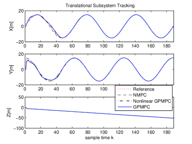
(a) Translational Subsystem Controlled Outputs

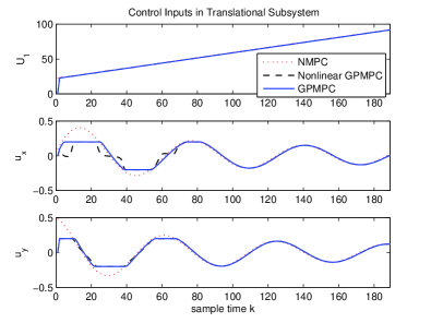
(b) Translational Subsystem Control Inputs

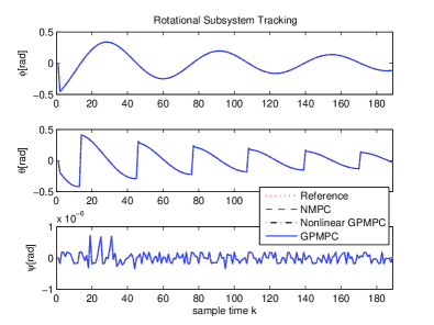
(c) Rotational Subsystem Controlled Outputs

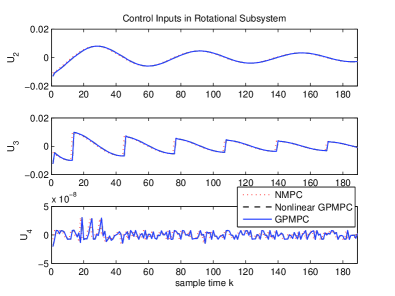
(d) Rotational Subsystem Control Inputs

Figure 2: Controlled outputs and control inputs by using the proposed GPMPC for the both two subsystems in the “Elliptical” trajectory

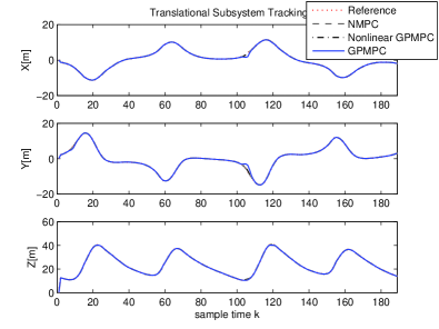
(a) Translational Subsystem Controlled Outputs

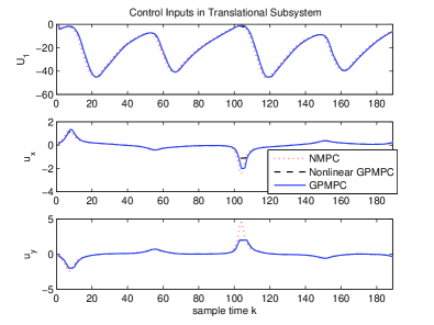
(b) Translational Subsystem Control Inputs

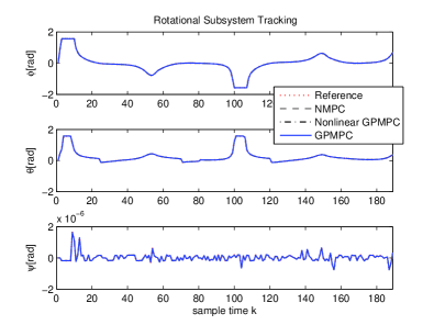
(c) Rotational Subsystem Controlled Outputs

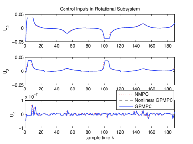
(d) Rotational Subsystem Control Inputs

Figure 3: Controlled outputs and control inputs by using the proposed GPMPC for the both two subsystems in the “Lorenz” trajectory

The gp models used in the control tasks are trained with all $\displaystyle 189$ observations because this ensures that the best quality models are obtained. The performance of using proposed GPMPC scheme is compared with using an exiting gp based mpc algorithm (referred to as “nonlinear GPMPC” or NMPC below) proposed in IC-Kocijan-MPCusingGP-2005 . Even though our optimization problem (19) with cost function (22) is more complicated than the one considered in IC-Kocijan-MPCusingGP-2005 , they are essentially similar. In addition, we choose $\displaystyle H=1$ as the prediction horizon. Theoretically, larger values of $\displaystyle H$ is necessary to guarantee the stability of mpc controllers. However, since solving the nonlinear GPMPC problem with larger values of $\displaystyle H$ effectively is an open problem, we restrict $\displaystyle H$ to be $\displaystyle 1$ in order to make proper comparisons. Our previous work in A-Gang-2016a has demonstrated that the proposed GPMPC can efficiently be used with a longer horizon.

The control results for the two trajectories are shown in Figures 2 and 3. They show that NMPC has the best tracking control performance. However, it should be noted that NMPC does not place any constraints on the control inputs. In general, the proposed GPMPC is able to closely follow the desired position and attitude values with constrained control inputs. The overall trajectory tracking results through using the GPMPC based hierarchical control scheme are depicted graphically in Figures 4(a) and 4(b).

Even with $\displaystyle H=1$, the nonlinear GPMPC requires $\displaystyle 220$ seconds and $\displaystyle 272$ seconds to compute all $\displaystyle 189$ control inputs for the “Elliptical” and “Lorenz” trajectory respectively. This is in contrast to the proposed GPMPC algorithm which only takes $\displaystyle 60$ seconds and $\displaystyle 56$ seconds. This demonstrates that the proposed GPMPC is computationally much more efficient than nonlinear GPMPC.

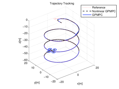
(a) “Elliptical”

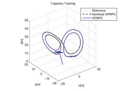
(b) “Lorenz”

Figure 4: The results of tracking “Elliptical” and “Lorenz” trajectories using the proposed control scheme

6 Conclusions

A new mpc algorithm is proposed for the quadrotor trajectory tracking problem where the quadrotor models are trained from empirical data using gp techniques. hierarchical control scheme based on a computationally efficient gp based for the quadrotor trajectory tracking problem. Models of the translational and rotational subsystems are learnt from collected data using gp modelling techniques rather than by traditional Newtonian analysis. The proposed GPMPC is able to computationally solve the resulting mpc tracking problems which are originally non-convex but can be reformulated as convex ones by using a linearisation of gp models. The numerical simulation results show that the proposed control scheme is able to closely track non-trivial trajectories. Its tracking performance is similar to using an nmpc method even though GPMPC has input constraints while no input constraints are placed on nmpc. In addition, compared to using an existing nonlinear GPMPC, the proposed GPMPC based control scheme has the advantage of solving the mpc problem much efficiently.

Appendix A

First rewrite (22) as follows:

$$\textit{E}\left[\mathcal{J}(\mathbf{x}_{k},\mathbf{u}_{k-1})\right]$$ (52)

$$=\textit{E}\Big{[}\sum_{i=1}^{H}\Big{\{}\big{\|}\mathbf{x}_{k+i}-\mathbf{r}_{k+i}\big{\|}^{2}_{\mathbf{Q}}+\big{\|}\mathbf{u}_{k+i-1}\big{\|}^{2}_{\mathbf{R}}\}\Big{]}$$

$$=\sum_{i=1}^{H}\bigg{\{}\underbrace{\textit{E}\Big{[}(\mathbf{x}_{k+i}-\mathbf{r}_{k+i})^{T}\mathbf{Q}(\mathbf{x}_{k+i}-\mathbf{r}_{k+i})\Big{]}}_{\text{probabilistic term}}$$

$$\quad\quad\quad+\underbrace{\mathbf{u}_{k+i-1}^{T}\mathbf{R}\mathbf{u}_{k+i-1}}_{\text{determinisitc term}}\bigg{\}}$$

Let $\displaystyle Q_{ab}$ be the entries of $\displaystyle\mathbf{Q}$ thus $\displaystyle Q_{ab}=[\mathbf{Q}]_{ab}$ and $\displaystyle\varepsilon_{ab}$ as the entries of $\displaystyle\bm{\Sigma}_{k}$ thus $\displaystyle\varepsilon_{ab}=[\bm{\Sigma}_{k}]_{ab}$, the “probabilistic term” can be further derived to

$$\textit{E}\Big{[}(\mathbf{x}_{k+i}-\mathbf{r}_{k+i})^{T}\mathbf{Q}(\mathbf{x}_{k+i}-\mathbf{r}_{k+i})\Big{]}$$ (53)

$$=\textit{E}\Big{[}\sum_{a=1}^{N}\sum_{b=1}^{N}Q_{ab}(\mathbf{x}_{k+i,a}-\mathbf{r}_{k+i,a})(\mathbf{x}_{k+i,b}-\mathbf{r}_{k+i,b})\Big{]}$$

$$=\sum_{a=1}^{N}\sum_{b=1}^{N}Q_{ab}\textit{E}\Big{[}(\mathbf{x}_{k+i,a}-\mathbf{r}_{k+i,a})(\mathbf{x}_{k+i,b}-\mathbf{r}_{k+i,b})\Big{]}$$

$$=\sum_{a=1}^{N}\sum_{b=1}^{N}Q_{ab}\bigg{\{}\textit{E}\big{[}\mathbf{x}_{k+i,a}-\mathbf{r}_{k+i,a}\big{]}\textit{E}\big{[}\mathbf{x}_{k+i,b}-\mathbf{r}_{k+i,b}\big{]}$$

$$\quad+\underbrace{\text{Cov}\bigg{(}(\mathbf{x}_{k+i,a}-\mathbf{r}_{k+i,a}),(\mathbf{x}_{k+i,b}-\mathbf{r}_{k+i,b})\bigg{)}}_{\varepsilon_{ab}}\bigg{\}}$$

$$=\sum_{a=1}^{N}\sum_{b=1}^{N}Q_{ab}\Big{\{}(\bm{\mu}_{k+i,a}-\mathbf{r}_{k+i,a})(\bm{\mu}_{k+i,a}-\mathbf{r}_{k+i,a})+\varepsilon_{ab}\Big{\}}$$

where

$$\sum_{a=1}^{N}\sum_{b=1}^{N}Q_{ab}(\bm{\mu}_{k+i,a}-\mathbf{r}_{k+i,a})(\bm{\mu}_{k+i,a}-\mathbf{r}_{k+i,a})$$ (54)

$$=(\bm{\mu}_{k+i}-\mathbf{r}_{k+i})^{T}\mathbf{Q}(\bm{\mu}_{k+i}-\mathbf{r}_{k+i})$$

and

$$\sum_{a=1}^{N}\sum_{b=1}^{N}Q_{ab}\varepsilon_{ab}=\textit{trace}(\mathbf{Q}\bm{\Sigma}_{k+i})$$ (55)

Therefore, (52) can be obtained by

$$\textit{E}\left[\mathcal{J}(\mathbf{x}_{k},\mathbf{u}_{k-1})\right]$$ (56)

$$=\sum_{i=1}^{H}\bigg{\{}(\bm{\mu}_{k+i}-\mathbf{r}_{k+i})^{T}\mathbf{Q}(\bm{\mu}_{k+i}-\mathbf{r}_{k+i})+\mathbf{u}_{k+i-1}^{T}\mathbf{R}\mathbf{u}_{k+i-1}$$

$$\quad+\textit{trace}(\mathbf{Q}\bm{\Sigma}_{k+i})\bigg{\}}$$

$$=\sum_{i=1}^{H}\Big{\{}\big{\|}\bm{\mu}_{k+i}-\mathbf{r}_{k+i}\big{\|}^{2}_{\mathbf{Q}}+\big{\|}\mathbf{u}_{k+i-1}\big{\|}^{2}_{\mathbf{R}}+\textit{trace}\big{(}\mathbf{Q}\bm{\Sigma}_{k+i}\big{)}\Big{\}}$$

References

• (1) Abdolhosseini, M., Zhang, Y., Rabbath, C.A.: An efficient model predictive control scheme for an unmanned quadrotor helicopter. Journal of Intelligent & Robotic Systems 70(1-4), 27–38 (2013)
• (2) Alexis, K., Nikolakopoulos, G., Tzes, A.: Switching model predictive attitude control for a quadrotor helicopter subject to atmospheric disturbances. Control Engineering Practice 19(10), 1195–1207 (2011)
• (3) Berkenkamp, F., Schoellig, A.P.: Learning-based robust control: Guaranteeing stability while improving performance. In: IEEE/RSJ Proceedings of International Conference on Intelligent Robots and Systems (IROS) (2014)
• (4) Bouabdallah, S., Noth, A., Siegwart, R.: PID vs LQ control techniques applied to an indoor micro quadrotor. In: IEEE/RSJ Proceedings of International Conference on Intelligent Robots and Systems (IROS), vol. 3, pp. 2451–2456. IEEE (2004)
• (5) Candela, J.Q., Girard, A., Larsen, J., Rasmussen, C.E.: Propagation of uncertainty in bayesian kernel models-application to multiple-step ahead forecasting. In: IEEE Proceedings of International Conference on Acoustics, Speech, and Signal Processing (ICASSP), vol. 2, pp. II–701. IEEE (2003)
• (6) Cao, G., Lai, E.M.K., Alam, F.: Gaussian process based model predictive control for linear time varying systems. In: International Workshop on Advanced Motion Control (AMC Workshop). IEEE (2016)
• (7) Cao, G., Lai, E.M.K., Alam, F.: Gaussian process model predictive control of unknown nonlinear systems. IET Control Theory & Applications (2016). URL https://arxiv.org/abs/1612.01211. Accepted for publication
• (8) Cao, G., Lai, E.M.K., Alam, F.: Gaussian process model predictive control of Unmanned Quadrotors. In: International Conference on Control, Automation and Robotics (ICCAR). IEEE (2016)
• (9) Deisenroth, M.P.: Efficient reinforcement learning using Gaussian processes. Ph.D. thesis, Karlsruhe Institute of Technology (2010)
• (10) Diehl, M., Ferreau, H.J., Haverbeke, N.: Efficient numerical methods for nonlinear MPC and moving horizon estimation. In: International Workshop on assessment and future directions on Nonlinear Model Predictive Control, pp. 391–417. Springer, Pavia, Italy (2008)
• (11) Dierks, T., Jagannathan, S.: Output feedback control of a quadrotor UAV using neural networks. IEEE Transactions on Neural Networks 21(1), 50–66 (2010)
• (12) Doherty, P., Rudol, P.: A UAV search and rescue scenario with human body detection and geolocalization. In: Advances in Artificial Intelligence, pp. 1–13. Springer (2007)
• (13) Fletcher, R.: Practical methods of optimization, second edn. Wiley-Interscience Publication (1987)
• (14) Girard, A., Rasmussen, C.E., Candela, J.Q., Murray-Smith, R.: Gaussian process priors with uncertain input – Application to multiple-step ahead time series forecasting. In: Advances in Neural Information Processing Systems (NIPS), pp. 545–552. MIT (2003)
• (15) Grancharova, A., Johansen, T.A., Tøndel, P.: Computational aspects of approximate explicit nonlinear model predictive control. In: Proceedings of the International Workshop on Assessment and Future Directions of Nonlinear Model Predictive Control, pp. 181–192. Springer (2007)
• (16) Grancharova, A., Kocijan, J., Johansen, T.A.: Explicit stochastic predictive control of combustion plants based on Gaussian process models. Automatica 44(6), 1621–1631 (2008)
• (17) Grüne, L., Pannek, J.: Nonlinear model predictive control–Theory and Algorithms. Springer-Verlag, London, U.K (2011)
• (18) Han, F., Feng, G., Wang, Y., Zhou, F.: Fuzzy modeling and control for a nonlinear quadrotor under network environment. In: IEEE 4th Annual International Conference on Cyber Technology in Automation Control, and Intelligent Systems (CYBER), pp. 395–400. IEEE (2014)
• (19) Hemakumara, P., Sukkarieh, S.: Non-parametric UAV system identification with dependent Gaussian processes. In: IEEE Proceedings of International Conference on Robotics and Automation (ICRA), pp. 4435–4441. IEEE (2011)
• (20) Hemakumara, P., Sukkarieh, S.: UAV parameter estimation with multi-output local and global Gaussian process approximations. In: IEEE Proceedings of International Conference on Robotics and Automation (ICRA), pp. 5402–5408. IEEE (2013)
• (21) Huang, M., Xian, B., Diao, C., Yang, K., Feng, Y.: Adaptive tracking control of underactuated quadrotor unmanned aerial vehicles via backstepping. In: American Control Conference, pp. 2076–2081. IEEE (2010)
• (22) Klenske, E.D., Zeilinger, M.N., Scholkopf, B., Hennig, P.: Gaussian process-based predictive control for periodic error correction. IEEE Transactions on Control Systems Technology (2015)
• (23) Kocijan, J., Murray-Smith, R.: Nonlinear predictive control with a Gaussian process model. In: In R. Murray-Smith and R. Shorten (eds.), Switching and Learning in Feedback Systems, pp. 185–200. Springer, Heidelberger, Berlin, Germany (2005)
• (24) Kocijan, J., Murray-Smith, R., Rasmussen, C.E., Girard, A.: Gaussian process model based predictive control. In: American Control Conference, vol. 3, pp. 2214–2219. IEEE (2004)
• (25) Kocijan, J., Murray-Smith, R., Rasmussen, C.E., Likar, B.: Predictive control with Gaussian process models. In: Proceedings of IEEE Region 8 EUROCON 2003:Computer As A Tool, vol. A, pp. 352–356. IEEE, Ljubljana (2003)
• (26) Likar, B., Kocijan, J.: Predictive control of a gas–liquid separation plant based on a Gaussian process model. Computers & Chemical Engineering 31(3), 142–152 (2007)
• (27) Liuzzi, G., Lucidi, S., Sciandrone, M.: Sequential penalty derivative-free methods for nonlinear constrained optimization. SIAM Journal on Optimization 20(5), 2614–2635 (2010)
• (28) Lucidi, S., Sciandrone, M., Tseng, P.: Objective-derivative-free methods for constrained optimization. Mathematical Programming 92(1), 37–59 (2002)
• (29) Madani, T., Benallegue, A.: Sliding mode observer and backstepping control for a quadrotor unmanned aerial vehicles. In: American Control Conference, pp. 5887–5892. IEEE (2007)
• (30) Mesbah, A.: Stochastic model predictive control: An overview and perspectives for future research. IEEE Control Systems Magazine, Accepted (2016)
• (31) Metni, N., Hamel, T.: A UAV for bridge inspection: Visual servoing control law with orientation limits. Automation in construction 17(1), 3–10 (2007)
• (32) Pan, Y., Theodorou, E.: Probabilistic differential dynamic programming. In: Advances in Neural Information Processing Systems (NIPS), pp. 1907–1915 (2014)
• (33) Quiñonero-Candela, J., Rasmussen, C.E.: A unifying view of sparse approximate Gaussian process regression. Journal of Machine Learning Research 6, 1939–1959 (2005)
• (34) Raffo, G.V., Ortega, M.G., Rubio, F.R.: An integral predictive/nonlinear H$\displaystyle\infty$ control structure for a quadrotor helicopter. Automatica 46(1), 29–39 (2010)
• (35) Rasmussen, C., Williams, C.: Gaussian Processes for Machine Learning. MIT Press, Cambridge, MA, USA (2006)
• (36) Valipour, M.: Application of new mass transfer formulae for computation of evapotranspiration. Journal of Applied Water Engineering and Research 2(1), 33–46 (2014)
• (37) Valipour, M.: How much meteorological information is necessary to achieve reliable accuracy for rainfall estimations $\displaystyle?$. Agriculture 6(4), 53 (2016)
• (38) Valipour, M.: Optimization of neural networks for precipitation analysis in a humid region to detect drought and wet year alarms. Meteorological Applications 23(1), 91–100 (2016)
• (39) Valipour, M.: Variations of land use and irrigation for next decades under different scenarios. IRRIGA:Brazilian Journal of Irrigation and Drainage 1(01), 262–288 (2016)
• (40) Valipour, M., Sefidkouhi, M.A.G., Raeini, M., et al.: Selecting the best model to estimate potential evapotranspiration with respect to climate change and magnitudes of extreme events. Agricultural Water Management 180, 50–60 (2017)
• (41) Voos, H.: Nonlinear and neural network-based control of a small four-rotor aerial robot. In: 2007 IEEE/ASME international conference on Advanced intelligent mechatronics, pp. 1–6. IEEE (2007)
• (42) Wang, Y., Boyd, S.: Fast model predictive control using online optimization. IEEE Transactions on Control Systems Technology 18(2), 267–278 (2010)
• (43) Yannopoulos, S.I., Lyberatos, G., Theodossiou, N., Li, W., Valipour, M., Tamburrino, A., Angelakis, A.N.: Evolution of water lifting devices (pumps) over the centuries worldwide. Water 7(9), 5031–5060 (2015)
• (44) Yiqing, L., Xigang, Y., Yongjian, L.: An improved PSO algorithm for solving non-convex NLP/MINLP problems with equality constraints. Computers & chemical engineering 31(3), 153–162 (2007)
• (45) Zuo, Z.: Trajectory tracking control design with command-filtered compensation for a quadrotor. IET Control Theory & Applications 4(11), 2343–2355 (2010)