Squark production in R-symmetric SUSY with Dirac gluinos: NLO corrections

Abstract

R-symmetry leads to a distinct realisation of SUSY with a significantly modified coloured sector featuring a Dirac gluino and a scalar colour octet (sgluon). We present the impact of R-symmetry on squark production at the 13 TeV LHC. We study the total cross sections and their NLO corrections from all strongly interacting states, their dependence on the Dirac gluino mass and sgluon mass as well as their systematics for selected benchmark points. We find that tree-level cross sections in the R-symmetric model are reduced compared to the MSSM but the NLO K-factors are generally larger in the order of ten to twenty per cent. In the course of this work we derive the required DREG $\to$ DRED transition counterterms and necessary on-shell renormalisation constants. The real corrections are treated using FKS subtraction, with results cross checked against an independent calculation employing the two cut phase space slicing method.

1 Introduction

The Minimal Supersymmetric Standard Model (MSSM) is one of the most studied extensions of the SM. Often, an unbroken R-parity is assumed which implies that supersymmetric particles can only be produced in pairs. In this paper we consider a distinct realisation of supersymmetry (SUSY) based on an unbroken, continuous R-symmetry. The basic feature of R-symmetry is that particles and superpartners have different R-charges where the differences are unambiguously prescribed by the SUSY algebra.

For definiteness we focus on the Minimal R-symmetric Supersymmetric Standard Model (MRSSM) Kribs:2007ac but our discussion will apply also to more general R-symmetric models.

From the phenomenological point of view, the MRSSM is an appealing model, with immediate restrictions following from R-symmetry. The model contains Dirac instead of Majorana gauginos and adjoint scalar superpartners for all gauge fields. This also leads to significant changes in the Higgs sector due to the presence of additional singlet and triplet scalars. The $\mu$- and $A$-terms of the MSSM are forbidden; mixing between left and right handed squarks or sleptons is forbidden, and large contributions to flavour and CP violating observables are suppressed Kribs:2007ac ; Dudas:2013gga .

In a recent series of papers, the electroweak sector has been investigated and it has been shown that the MRSSM can accommodate the experimentally measured $W$ and Higgs boson mass as well as the electroweak precision variables and is compatible with direct detection searches for dark matter and LHC searches of electroweak particles Diessner:2014ksa ; Diessner:2015yna . For related studies, see Braathen:2016mmb ; Nakano:2015gws ; Ding:2015epa .

In this paper we focus on the strongly interacting sector of R-symmetric SUSY. It is characterised by Dirac gluinos, scalar gluons and left and right handed squarks which are mass eigenstates and have opposite R-charges. The phenomenology of this SUSY QCD sector of the MRSSM has already been studied at the tree level Heikinheimo:2011fk ; Kribs:2013oda , where it was shown that conservation of R-charge is responsible for a rather drastic suppression of the inclusive squark production cross section leading to lower bounds on squark masses. This suppression is even more amplified when the gluino mass is increased. Corrections to this observable at the next-to-leading order (NLO) have only been approximately estimated in ref. Kribs:2012gx by using global MSSM instead of MRSSM K-factors. It is the purpose of this paper to describe an exact NLO SUSY-QCD calculation in the MRSSM at the example of squark-squark ($\tilde{q}\tilde{q}$) and squark-antisquark ($\tilde{q}\tilde{q}^{\dagger}$) production at the LHC. We will expose and explain differences to the analogous calculation in the MSSM.

The paper is structured as follows. The next section describes the strongly interacting sector of the MRSSM. In section 3 we evaluate the leading order cross sections for the production of colour charged MRSSM particles. Section 4 describes the evaluation and renormalisation of the virtual amplitudes. Our results have been obtained with two independent codes which use different regularisation schemes Signer:2008va . We provide a list of counterterms including the transition counterterm from dimensional regularisation to dimensional reduction. Section 5 is devoted to the description of real corrections. We present two alternative ways of dealing with infrared singularities used in this work: the two cut phase space slicing method and the FKS subtraction. We also discuss the treatment of the on-shell resonances. In section 6 we proceed with a phenomenological analysis. We give a detailed comparison of K-factors in the MSSM and the MRSSM, explaining the physical origins of their differences. Then we give an overview of the NLO corrected cross sections in different regions of parameter space, including an uncertainty discussion. Section 7 contains our conclusions, and the appendix collects a list of Feynman rules, implementation details, and numerical results for verification purposes.

2 Details of the model

The field content of the MRSSM is enlarged in comparison to the one of the MSSM. The necessity of this arises from R-symmetry. As can be seen from table 1 the gluino $\tilde{g}_{L}$, as superpartner of the gluon, has R-charge $+1$. In order to account for a non-vanishing Dirac gluino mass it needs to be partnered with a new field $\tilde{g}_{R}$ with R-charge $-1$. The Dirac nature of gluinos manifests itself in an $N=2$ supersymmetric gauge sector including scalar gluons $O$, called sgluons, which transform in the same representation as the gluon under gauge transformations.

superfield		boson		fermion
left-handed (s)quark	$\widehat{Q}_{L}$	$\tilde{q}_{L}$	$1$	$q_{L}$	$0$
right-handed (s)quark	$\widehat{Q}_{R}$	$\tilde{q}_{R}^{\dagger}$	$1$	$\bar{q}_{R}$	$0$
gluon vector superfield	$\widehat{V}$	$g$	0	$\tilde{g}_{L}$	$+1$
adjoint chiral superfield	$\widehat{O}$	$O$	$0$	$\tilde{g}_{R}$	$-1$

Table 1: The table shows the strongly interacting field content of the MRSSM, together with the R-charges of the component fields. The superfield in the last line is absent in the MSSM. It comprises of the right-handed component of the Dirac gluino and two real sgluons.

The corresponding Lagrangian of the strongly interacting part of the MRSSM, including one massless quark of arbitrary flavour reads

$$\mathcal{L}_{\mathrm{RSQCD}}= \int\mathrm{d}^{4}\theta\ \left(\widehat{\overline{Q}}_{L}\mathrm{e}^{2g_{s}\widehat{V}_{s}}\widehat{Q}_{L}+\widehat{\overline{Q}}_{R}\mathrm{e}^{-2g_{s}\widehat{V}^{T}_{s}}\widehat{Q}_{R}+\widehat{\overline{O}}\mathrm{e}^{2g_{s}\widehat{V}^{\mathrm{adj.}}_{s}}\widehat{O}\right)$$

$$+ \left(\int\mathrm{d}^{2}\theta\frac{1}{16g_{s}^{2}}\widehat{W}_{s}^{a\alpha}\widehat{W}^{a}_{s\alpha}+h.c.\right)+\mathcal{L}_{\mathrm{soft}}\,.$$ (1)

Note that the vector superfield of the gluon $\widehat{V}_{s}$ in the first line of eq. (1) transforms for each term in the appropriate representation of $SU(3)_{C}$, i.e. the fundamental, the antifundamental and the adjoint one.
The soft breaking Lagrangian accounts for squark, gaugino and sgluon masses. These mass terms arise from a hidden sector spurion. For gauginos the D-type spurion is given by $\widehat{W}_{\alpha}^{\prime}=\theta_{\alpha}D$ and mediates supersymmetry breaking at the mediation scale $M$: $\int\mathrm{d}\theta^{2}\frac{\widehat{W}_{\alpha}^{\prime}}{M}\widehat{W}_{s}^{\alpha}\widehat{O}$. After integrating out the spurion one obtains Fox:2002bu ; Diessner:2014ksa

$$\mathcal{L}_{\mathrm{soft}}=\ -\frac{m_{\tilde{q}_{L}}^{2}}{2}|\tilde{q}_{L}|^{2}-\frac{m_{\tilde{q}_{R}}^{2}}{2}|\tilde{q}_{R}|^{2}$$

$$-m_{O}^{2}\left|O^{a}\right|^{2}-m_{\tilde{g}}\left(\overline{\tilde{g}_{R}}\tilde{g}_{L}-\sqrt{2}D^{a}O^{a}+\text{h.c.}\right)\;,$$ (2)

where $D^{a}$ is the usual auxiliary field in the $SU(3)$ sector. The complex sgluon state has to be decomposed into two real fields:

$$O=\frac{O_{s}+iO_{p}}{\sqrt{2}}\,.$$ (3)

The mass of the CP-even scalar $O_{s}$ receives an additional contribution from the gluino Dirac mass whereas the mass of the pseudoscalar $O_{p}$ is solely given by the soft breaking parameter:

$$m_{O_{s}}=\sqrt{m_{O}^{2}+4m_{\tilde{g}}^{2}}\;,\quad m_{O_{p}}=m_{O}\,.$$ (4)

The respective Feynman rules derived from this Lagrangian differ partly from the ordinary MSSM ones. Those Feynman rules which have no MSSM counterpart are listed in appendix A.

To study the relevant SUSY-QCD effects of the MRSSM quantitatively, we define three benchmark points given in table 2.

	$m_{\tilde{q}}$	$m_{\tilde{g}}$	$m_{\tilde{O}_{s}}$	$m_{\tilde{O}_{p}}$
BM1	1500	1000	5385	5000
BM2	1500	2000	6403	5000
BM3	500	2000	6403	5000

Table 2: Benchmark points. Assuming unified squark masses and the sgluon masses apply only to the MSSM. All masses are given in GeV.

3 Squark and gluino production at the leading order

As a starting point for the NLO SUSY-QCD calculation, we recall the tree-level production of squarks and gluinos in the MRSSM and point out differences to the familiar MSSM. A detailed study including comparisons of Dirac, Majorana and hybrid gluinos can be found in ref. Choi:2008pi . As in the MSSM there are six partonic channels contributing to squark and gluino production. Three of which for squark-antisquark and squark-squark production

$$q_{i}\overline{q}_{j}\to\tilde{q}_{k}\tilde{q}_{l}^{\dagger},\hskip 28.45274ptgg\to\tilde{q}_{i}\tilde{q}_{i}^{\dagger},\hskip 28.45274ptq_{i}q_{j}\to\tilde{q}_{i}\tilde{q}_{j}\hskip 14.22636pt.$$ (5)

and three for gluino-antigluino and squark-(anti)gluino production

$$q_{i}\overline{q}_{i}\to\tilde{g}\overline{\tilde{g}},\hskip 28.45274ptgg\to\tilde{g}\overline{\tilde{g}},\hskip 28.45274ptq_{i}g\to\tilde{q}_{i}\tilde{g}\ /\ \tilde{q}_{i}\overline{\tilde{g}}\hskip 14.22636pt.$$ (6)

The inclusion of charge conjugated processes is understood if they exist. The indices denote quark flavours. The corresponding Feynman diagrams are shown in figure 1.

Figure 1: Tree-level diagrams for squark and gluino production in the MRSSM. For simplicity, only one quark flavour is shown. In the third and last line, also a charge conjugated process exists.

In the following we give analytic formulae for the partonic cross sections for several channels in the MRSSM and explain if/how they differ to their respective analogue in the MSSM. We sum over the $n_{f}-1$ first (s)quark flavours (where $n_{f}\equiv 6$). The gauge coupling $g_{s}$ from the $qqg$-vertex is identical to its supersymmetric analogue $\hat{g}_{s}$ from the $q\tilde{q}\tilde{g}$-vertex. Taking all squarks as mass degenerate, we obtain the leading order partonic cross sections

$$\hat{\sigma}^{B}(q_{i}\overline{q}_{j}\to\tilde{q}\tilde{q}^{\dagger}) =\delta_{ij}\frac{g_{s}^{4}}{16\pi\hat{s}}(n_{f}-1)\left[\frac{4}{27}-\frac{16m_{\tilde{q}}^{2}}{27\hat{s}}\right]\beta_{\tilde{q}}$$

$$+\delta_{ij}\frac{g_{s}^{2}\hat{g}_{s}^{2}}{16\pi\hat{s}}\left[\left(\frac{4}{27}+\frac{8m_{-}^{2}}{27\hat{s}}\right)\beta_{\tilde{q}}+\left(\frac{8m_{\tilde{g}}^{2}}{27\hat{s}}+\frac{8m_{-}^{4}}{27\hat{s}^{2}}\right)L_{1}\right]$$

$$+\frac{\hat{g}_{s}^{4}}{16\pi\hat{s}}\left[-\frac{8}{9}\beta_{\tilde{q}}+\left(-\frac{4}{9}-\frac{8m_{-}^{2}}{9\hat{s}}\right)L_{1}\right],$$ (7)

$$\hat{\sigma}^{B}(gg\to\tilde{q}\tilde{q}^{\dagger}) =\frac{(n_{f}-1)g_{s}^{4}}{16\pi\hat{s}}\left[\left(\frac{5}{24}+\frac{31m_{\tilde{q}}^{2}}{12\hat{s}}\right)\beta_{\tilde{q}}+\left(\frac{4m_{\tilde{q}}^{2}}{3\hat{s}}+\frac{m_{\tilde{q}}^{4}}{3\hat{s}^{2}}\right)\ln\frac{1-\beta_{\tilde{q}}}{1+\beta_{\tilde{q}}}\right],$$ (8)

$$\hat{\sigma}^{B}(q_{i}q_{j}\to\tilde{q}\tilde{q}) =\frac{\hat{g}_{s}^{4}}{16\pi\hat{s}}\left[-\frac{8}{9}\beta_{\tilde{q}}+\left(-\frac{4}{9}-\frac{8m_{-}^{2}}{9\hat{s}}\right)L_{1}\right],$$ (9)

$$\hat{\sigma}^{B}(q\overline{q}\to\tilde{g}\overline{\tilde{g}}) =\frac{g_{s}^{4}}{16\pi\hat{s}}\left[\frac{16}{9}+\frac{32m_{\tilde{g}}^{2}}{9\hat{s}}\right]\beta_{\tilde{g}}$$

$$+\frac{\hat{g}_{s}^{2}g_{s}^{2}}{16\pi\hat{s}}\left[\left(-\frac{4}{3}-\frac{8m_{-}^{2}}{3\hat{s}}\right)\beta_{\tilde{g}}+\left(\frac{8m_{\tilde{g}}^{2}}{3\hat{s}}+\frac{8m_{-}^{4}}{3\hat{s}^{2}}\right)L_{2}\right]$$

$$+\frac{\hat{g}_{s}^{4}}{16\pi\hat{s}}\left[\left(\frac{32}{27}+\frac{32m_{-}^{4}}{m_{-}^{4}+m_{\tilde{q}}^{2}\hat{s}}\right)\beta_{\tilde{g}}-\frac{64m_{-}^{2}}{27\hat{s}}L_{2}\right],$$ (10)

$$\hat{\sigma}^{B}(gg\to\tilde{g}\overline{\tilde{g}}) =\frac{g_{s}^{4}}{16\pi\hat{s}}\left[\left(-6-\frac{51m_{\tilde{g}}^{2}}{2\hat{s}}\right)\beta_{\tilde{g}}+\left(-\frac{9}{2}-\frac{18m_{\tilde{g}}^{2}}{\hat{s}}+\frac{18m_{\tilde{g}}^{4}}{\hat{s}^{2}}\right)\ln\frac{1-\beta_{\tilde{g}}}{1+\beta_{\tilde{g}}}\right],$$ (11)

$$\hat{\sigma}^{B}(qg\to\tilde{q}\tilde{g}) =\frac{g_{s}^{2}\hat{g}_{s}^{2}}{16\pi\hat{s}}\left[\frac{\kappa}{\hat{s}}\left(-\frac{7}{9}-\frac{32m_{-}^{2}}{9\hat{s}}\right)+\left(-\frac{8m_{-}^{2}}{9\hat{s}}+\frac{2m_{\tilde{q}}^{2}m_{-}^{2}}{\hat{s}^{2}}+\frac{8m_{-}^{4}}{9\hat{s}^{2}}\right)L_{3}\right.$$

$$+\left.\left(-1-\frac{2m_{-}^{2}}{\hat{s}}+\frac{2m_{\tilde{q}}m_{-}^{2}}{\hat{s}^{2}}\right)L_{4}\right]\,,$$ (12)

where $\hat{s}$ is the squared partonic centre-of-mass energy and the following abbreviations of ref. Beenakker:1996ch are used

$$\beta_{\tilde{q}}=\sqrt{1-\frac{4m_{\tilde{q}}^{2}}{\hat{s}}}, \beta_{\tilde{g}}=\sqrt{1-\frac{4m_{\tilde{g}}^{2}}{\hat{s}}},$$

$$m_{-}^{2}=m_{\tilde{g}}^{2}-m_{\tilde{q}}^{2}, \kappa=\sqrt{(\hat{s}-m_{\tilde{g}}^{2}-m_{\tilde{q}}^{2})^{2}-4m_{\tilde{g}}^{2}m_{\tilde{q}}^{2}},$$

$$L_{1}=\ln\frac{\hat{s}+2m_{-}^{2}-\hat{s}\beta_{\tilde{q}}}{\hat{s}+2m_{-}^{2}+\hat{s}\beta_{\tilde{q}}}, L_{2}=\ln\frac{\hat{s}-2m_{-}^{2}-\hat{s}\beta_{\tilde{g}}}{\hat{s}-2m_{-}^{2}+\hat{s}\beta_{\tilde{g}}},$$

$$L_{3}=\ln\frac{\hat{s}-m_{-}^{2}-\kappa}{\hat{s}-m_{-}^{2}+\kappa}, L_{4}=\ln\frac{\hat{s}+m_{-}^{2}-\kappa}{\hat{s}+m_{-}^{2}+\kappa}\;.$$ (13)

In comparison to the MSSM there are two main differences. Firstly, an overall restriction stemming from an unbroken R-symmetry is that the final state particles’ R-charges must sum up to zero. Hence in the MRSSM, only diagrams for $q\overline{q}\to\tilde{q}_{L}\tilde{q}_{L}^{\dagger}$, $q\overline{q}\to\tilde{q}_{R}\tilde{q}_{R}^{\dagger}$ and $qq\to\tilde{q}_{L}\tilde{q}_{R}$ can be drawn as shown in figure 1. Processes with a squark-antisquark (squark-squark) pair of different (same) “chiralities” in the final state are forbidden by R-symmetry.

For the allowed channels in the MRSSM the chirality projectors lead to the replacement

$$\frac{\not{p}+m_{\tilde{g}}}{p^{2}-m_{\tilde{g}}^{2}}\to\frac{\not{p}}{p^{2}-m_{\tilde{g}}^{2}}$$ (14)

for the gluino propagator in the first and third line of figure 1. On the level of the cross section, this manifests in the substitution

$$\frac{\hat{g}_{s}^{4}}{16\pi^{2}\hat{s}}\left(-\frac{4}{9}-\frac{4m_{-}^{4}}{9(m_{\tilde{g}}^{2}\hat{s}+m_{-}^{4})}\right)\beta_{\tilde{q}}\to-\frac{\hat{g}_{s}^{4}}{16\pi^{2}\hat{s}}\cdot\frac{8}{9}\beta_{\tilde{q}}$$ (15)

and the vanishing of the term proportional to $\delta_{ij}$ for $\tilde{q}\tilde{q}$ production in ref. Beenakker:1996ch , compared to the MSSM expressions. Expanding $\hat{\sigma}^{B}(q_{i}q_{j}\to\tilde{q}\tilde{q})$ appropriately for large values of $m_{\tilde{g}}$, shows that the leading term in the MSSM is proportional to $m_{\tilde{g}}^{-2}$, whereas in the MRSSM it is $m_{\tilde{g}}^{-4}$, as expected from eq. (14).

A second feature of the MRSSM is that gluino and antigluino are no longer indistinguishable particles, which manifests in twice as much degrees of freedom available for the gluino in the final state. In contrast to the above mentioned feature, this characteristic induces an increase of some cross sections. It strikes very clearly in the cross section of $gg\to\tilde{g}\overline{\tilde{g}}$, which is doubled in comparison to the MSSM. For the process $q\overline{q}\to\tilde{g}\overline{\tilde{g}}$, both features appear: The first line of eq. (10) is twice as much as its MSSM analogue in ref. Beenakker:1996ch but the following two are not. This is because those originate from $t$- and $u$-channel diagrams where only one instead of two squark “chiralities” occur. In addition, the MRSSM result misses the $t$- and $u$-channel interference. In the last channel, i.e. $qg\to\tilde{q}\tilde{g}$, both features are present and cancel exactly. On the one hand, R-charge allows only the production of “right-handed” squarks in association with the gluino. On the other hand, there is a distinct antigluino which can be produced with a “left-handed” squark. As for $\tilde{q}\tilde{q}$ production, the charge conjugated process exists.

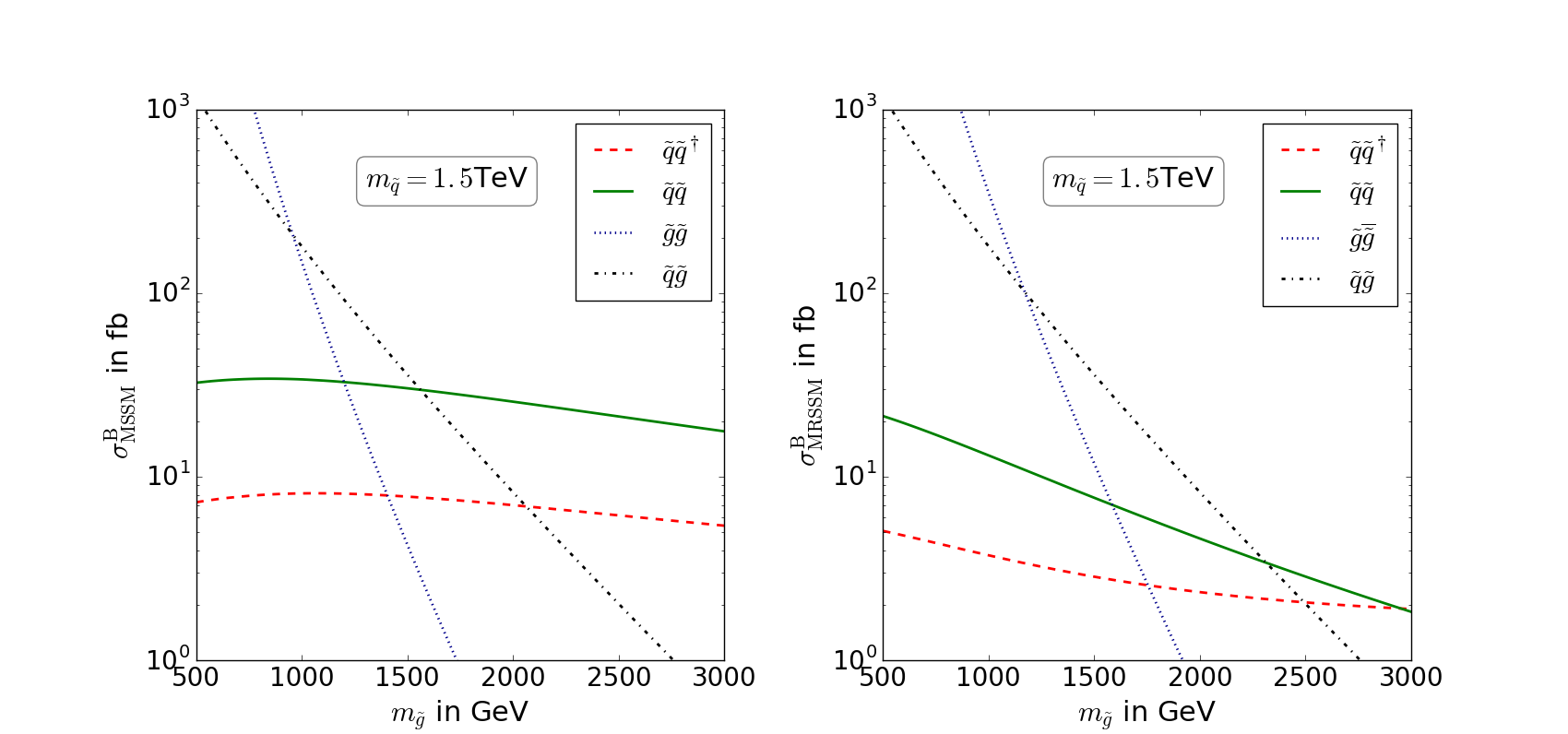
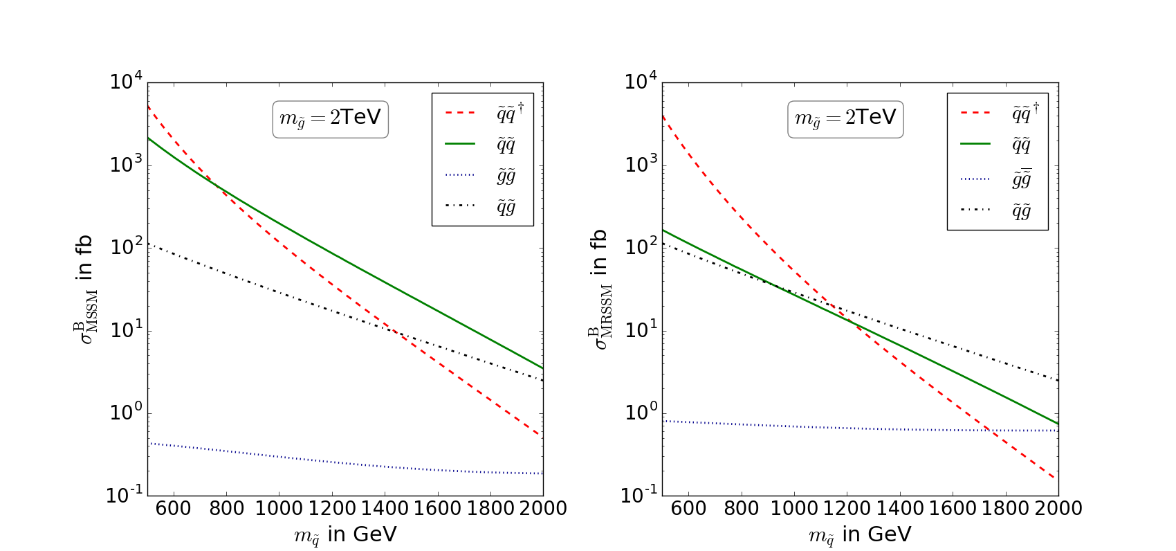
Figure 2: The production cross sections for squarks and gluinos at the LHC with $\sqrt{S}=13\,\mathrm{TeV}$ in the MSSM (left) and the MRSSM (right). It is summed over five flavours, all possible squark “chiralities” and for squark-squark and squark-gluino production also the charge conjugated processes are taken into account. The top row contains results in function of the gluino mass (with squark masses fixed to 1.5 TeV), the bottom one in function of squark masses with the gluino mass fixed to 2 TeV. The PDF set used is $\mathtt{MMHT2014LO}$ Harland-Lang:2014zoa . As renormalisation and factorisation scale $\mu_{R}=\mu_{F}=\frac{m_{1}+m_{2}}{2}$ has been chosen, where $m_{i}$ are the final state’s particle masses.

In conclusion, we obtain both suppressing as well as amplifying effects in the MRSSM. In contrast to the Dirac gluino, the presence of sgluons has no effect on the discussed tree-level processes. Figure 2 shows the convolution of the partonic cross sections with parton distribution functions (PDFs) in the MSSM and the MRSSM for the 13 TeV LHC. For details regarding the parameters used, see the caption of figure 2. We sum over all “chiralities” and five flavours as well as charge conjugated processes, when distinct. Due to the prohibition of the above mentioned “chirality” states in the MRSSM, we obtain a suppression in the $\tilde{q}\tilde{q}^{\dagger}$ and $\tilde{q}\tilde{q}$ production (by a factor of 1.3 and 13.2 at BMP2, respectively), which increases with the gluino mass. Furthermore, an amplification of gluino production, due to its Dirac nature, is visible. In combination with experimental results, the absence of detected gluinos translates into a larger exclusion limit of the gluino mass than in SUSY-QCD Heikinheimo:2011fk . We will thus focus on the region of parameter space with a rather large gluino mass when discussing our NLO results.

4 Virtual corrections

The present and the subsequent sections describe the calculation of the NLO SUSY-QCD corrections to squark production processes in the MRSSM. The inclusion of gluino final states we postpone for future work, since they are not as important in the motivated scenario where squarks are significantly lighter than gluinos. Thus, on hadron level we consider squark-squark production $pp\to\tilde{q}\tilde{q}$ and squark-antisquark production $pp\to\tilde{q}\tilde{q}^{\dagger}$. On the partonic level we have to consider NLO corrections to $qq\to\tilde{q}\tilde{q}$ for the first process and NLO corrections to $q\overline{q}\to\tilde{q}\tilde{q}^{\dagger}$ and $gg\to\tilde{q}\tilde{q}^{\dagger}$ for the second process.

In the present section we focus on the virtual corrections. They involve ultraviolet and soft and collinear infrared divergences. These divergences are removed after renormalisation and combination with real corrections.

In intermediate steps, the divergences need to be regularised. However, computations of SUSY-QCD corrections suffer from the fact that no regularisation is at the same time directly compatible with SUSY and the standard definition of PDFs, see also ref. Signer:2008va and ref. Gnendiger:2017pys for a recent review. Hence we have done the calculation in two complementary ways.

• The first calculation uses dimensional regularisation (version HV in the notation of ref. Signer:2008va ) and Passarino-Veltman reduction of one-loop integrals. In the HV scheme all four-dimensional quantities are treated in $D=4-2\epsilon$ dimensions, except that particles outside loops are kept unregularised. In this calculation SUSY is broken in intermediate steps and SUSY-restoring counterterms must be added.

• The second calculation uses dimensional reduction/the four-dimensional helicity scheme (version FDH in the notation of ref. Signer:2008va ), helicity methods and integrand reduction techniques. In the FDH scheme, only space-time and momenta are treated in $D$ dimensions, while gluons are kept quasi-four-dimensional. Like in HV, only particles inside loops are regularised. In this calculation a finite shift is needed in the strong coupling renormalisation, and transition rules have to be applied to convert infrared divergent amplitudes back to the HV scheme.

The two calculations are in full agreement. In the following we provide the details, first on the general renormalisation scheme, then on the two calculational procedures.

4.1 One-loop diagrams and renormalisation

a)

b)

c)

Figure 3: Examples of Feynman diagrams relevant for the calculation of the counterterms. Category a) diagrams are as in the MSSM. For comparison category b) contains diagrams which lead to contributions in the MSSM but not the MRSSM. Category c) are novel diagrams originating from the sgluons.

a)

b)

c)

Figure 4: Examples of Feynman diagrams relevant for the NLO corrections to $\tilde{q}\tilde{q}$ and $\tilde{q}\tilde{q}^{\dagger}$ production. Categories as in figure 3.

We need to consider the one-loop amplitudes for the three partonic processes $q\overline{q}\to\tilde{q}\tilde{q}^{\dagger}$, $gg\to\tilde{q}\tilde{q}^{\dagger}$, and $qq\to\tilde{q}\tilde{q}$. Sample Feynman diagrams for the calculation of renormalisation constants are shown in figure 3. Diagrams contributing to the production of (anti)squarks are shown in figure 4. Diagrams of type a) are exactly the same in the MRSSM and in the conventional MSSM and give equal results. Diagrams of type b) can be drawn in the MRSSM but unlike in the MSSM do not contribute. The result is proportional to the Majorana mass and leads therefore to R-charge violation in the MRSSM. Diagrams of type c) exist in the MRSSM but are absent in the MSSM because of the appearance of sgluons, additional strongly interacting particles.

The ultraviolet renormalisation requires the introduction of coupling, mass, and field renormalisation. We define all SUSY masses in the on-shell renormalisation scheme to have physical masses as input. The quark masses are set to zero, except for the top quark mass. For simplicity we take all squarks as mass degenerate. We define the field renormalisation in the on-shell scheme, which leads to a correctly normalised S-matrix but also to infrared divergent renormalisation constants. The strong coupling is renormalised in a decoupling scheme as described below.

With these definitions, standard methods lead to the following results for the quark/squark field and squark mass renormalisation constants, computed with one-loop SUSY-QCD corrections:

$$\delta Z_{q} =2C_{F}\frac{g_{s}^{2}}{16\pi^{2}}\Re\left[B_{1}(0,m_{\tilde{g}}^{2},m_{\tilde{q}}^{2})\right]\,,$$ (16)

$$\delta Z_{\tilde{q}} =\frac{g_{s}^{2}}{16\pi^{2}}C_{F}\Re\left[4B_{1}(m_{\tilde{q}}^{2},0,m_{\tilde{g}}^{2})+2B_{1}(m_{\tilde{q}}^{2},0,m_{\tilde{q}}^{2})+3B_{0}(m_{\tilde{q}}^{2},0,m_{\tilde{q}}^{2})+4m_{\tilde{q}}^{2}B^{\prime}_{1}(m_{\tilde{q}}^{2},0,m_{\tilde{g}}^{2})\right.$$

$$\left.-4m_{\tilde{g}}^{2}B^{\prime}_{0}(m_{\tilde{q}}^{2},m_{O_{s}}^{2},m_{\tilde{q}}^{2})+2m_{\tilde{q}}^{2}B^{\prime}_{1}(m_{\tilde{q}}^{2},0,m_{\tilde{q}}^{2})+4m_{\tilde{q}}^{2}B^{\prime}_{0}(m_{\tilde{q}}^{2},0,m_{\tilde{q}}^{2})\right]\,,$$ (17)

$$\delta m_{\tilde{q}}^{2} =\frac{g_{s}^{2}}{16\pi^{2}}C_{F}\Re\left[A_{0}(m_{\tilde{q}}^{2})-(4A_{0}(m_{\tilde{g}}^{2})+4B_{1}(m_{\tilde{q}}^{2},0,m_{\tilde{g}}^{2})m_{\tilde{q}}^{2})+4m_{\tilde{g}}^{2}B_{0}(m_{\tilde{q}}^{2},m_{O_{s}}^{2},m_{\tilde{q}}^{2})\right.$$

$$\left.-(2B_{1}(m_{\tilde{q}}^{2},0,m_{\tilde{q}}^{2})m_{\tilde{q}}^{2}+4B_{0}(m_{\tilde{q}}^{2},0,m_{\tilde{q}}^{2})m_{\tilde{q}}^{2})\right]\,.$$ (18)

We use standard Passarino-Veltman integrals and their derivatives, see e.g. ref. Denner:1991kt for the definition. The renormalisation constants are computed in both the HV and FDH scheme; we denote terms only appearing in HV by the subscript HV. We do not have to distinguish left- and right-handed squarks since we do not take electroweak corrections into account.

Though not strictly necessary for our calculations, we also quote the result for the gluino field renormalisation. Here the left- and right-handed parts renormalise differently, since they are part of different superfields, i.e. the right-handed part of the gluino does not couple to (s)quarks. This is reflected by a gluino self-energy which is not left-right symmetric and has the following basic structure:

$$\Sigma^{\mathrm{MRSSM}}_{\tilde{g}\overline{\tilde{g}}}(p^{2}) =A(p^{2})P_{L}\not{p}+\ldots,$$ (19)

$$\Sigma^{\mathrm{MSSM}}_{\tilde{g}\overline{\tilde{g}}}(p^{2}) =A(p^{2})(P_{L}+P_{R})\not{p}+\ldots,$$ (20)

where the dots stand for contributions not stemming from (s)quarks. The results read

$$\delta Z_{\tilde{g}}^{R} =\frac{g_{s}^{2}}{16\pi^{2}}\Re\left[C_{A}(B_{1}(m_{\tilde{g}}^{2},m_{\tilde{g}}^{2},m_{O_{s}}^{2})+B_{1}(m_{\tilde{g}}^{2},m_{\tilde{g}}^{2},m_{O_{p}}^{2}))\right.$$

$$+C_{A}(\left.1\right|_{\texttt{HV}}-2(B_{0}(m_{\tilde{g}}^{2},0,m_{\tilde{g}}^{2})+B_{1}(m_{\tilde{g}}^{2},0,m_{\tilde{g}}^{2})))$$

$$+4T_{F}m_{\tilde{g}}^{2}\left((n_{f}-1)B^{\prime}_{1}(m_{\tilde{g}}^{2},0,m_{\tilde{q}}^{2})+B^{\prime}_{1}(m_{\tilde{g}}^{2},m_{t}^{2},m_{\tilde{q}}^{2})\right)$$

$$-2C_{A}m_{\tilde{g}}^{2}\left(B^{\prime}_{0}(m_{\tilde{g}}^{2},m_{\tilde{g}}^{2},m_{O_{s}}^{2})-B^{\prime}_{0}(m_{\tilde{g}}^{2},m_{\tilde{g}}^{2},m_{O_{p}}^{2})-B^{\prime}_{1}(m_{\tilde{g}}^{2},m_{\tilde{g}}^{2},m_{O_{s}}^{2})-B^{\prime}_{1}(m_{\tilde{g}}^{2},m_{\tilde{g}}^{2},m_{O_{p}}^{2})\right)$$

$$+4C_{A}m_{\tilde{g}}^{2}\left.\left(B^{\prime}_{0}(m_{\tilde{g}}^{2},0,m_{\tilde{g}}^{2})-B^{\prime}_{1}(m_{\tilde{g}}^{2},0,m_{\tilde{g}}^{2})\right)\right]\,,$$ (21)

$$\delta Z_{\tilde{g}}^{L} =\frac{g_{s}^{2}}{16\pi^{2}}\Re\left[4T_{F}\left((n_{f}-1)B_{1}(m_{\tilde{g}}^{2},0,m_{\tilde{q}}^{2})+B_{1}(m_{\tilde{g}}^{2},m_{t}^{2},m_{\tilde{q}}^{2})\right)\right]+\delta Z_{\tilde{g}}^{R}\,.$$ (22)

The corresponding gluino mass renormalisation constant is

$$\delta m_{\tilde{g}} =\frac{g_{s}^{2}}{16\pi^{2}}m_{\tilde{g}}\ \Re\left[-2T_{F}\left((n_{f}-1)B_{1}(m_{\tilde{g}}^{2},0,m_{\tilde{q}}^{2})+B_{1}(m_{\tilde{g}}^{2},m_{t}^{2},m_{\tilde{q}}^{2})\right)\right.$$

$$+C_{A}\left(B_{0}(m_{\tilde{g}}^{2},m_{\tilde{g}}^{2},m_{O_{s}}^{2})-B_{0}(m_{\tilde{g}}^{2},m_{\tilde{g}}^{2},m_{O_{p}}^{2})-B_{1}(m_{\tilde{g}}^{2},m_{\tilde{g}}^{2},m_{O_{s}}^{2})-B_{1}(m_{\tilde{g}}^{2},m_{\tilde{g}}^{2},m_{O_{p}}^{2})\right)$$

$$+C_{A}\left.\left(\left.1\right|_{\texttt{HV}}-2B_{0}(m_{\tilde{g}}^{2},0,m_{\tilde{g}}^{2})+2B_{1}(m_{\tilde{g}}^{2},0,m_{\tilde{g}}^{2})\right)\right]\,.$$ (23)

Note that the contribution stemming from the quark-squark loop is halved when compared to the MSSM result, due to the non-coupling right-handed gluino. As a consequence, the left-handed Dirac gluino allows only for a “left-handed” squark or a “right-handed” antisquark in the loop. Finally, the field renormalisation constant of the gluon is given by

$$\delta Z_{G} =\frac{g_{s}^{2}}{16\pi^{2}}\Re\left[T_{F}\left(-\frac{4}{3}B_{0}(0,m_{t}^{2},m_{t}^{2})-\frac{8}{3}m_{t}^{2}B^{\prime}_{0}(0,m_{t}^{2},m_{t}^{2})+\frac{4}{9}\right)\right.$$

$$+C_{A}\left(-\frac{4}{3}B_{0}(0,m_{\tilde{g}}^{2},m_{\tilde{g}}^{2})-\frac{8}{3}m_{\tilde{g}}^{2}B^{\prime}_{0}(0,m_{\tilde{g}}^{2},m_{\tilde{g}}^{2})+\frac{4}{9}\right)$$

$$+12T_{F}\left(-\frac{1}{3}B_{0}(0,m_{\tilde{q}}^{2},m_{\tilde{q}}^{2})+\frac{4}{3}m_{\tilde{q}}^{2}B^{\prime}_{0}(0,m_{\tilde{q}}^{2},m_{\tilde{q}}^{2})-\frac{2}{9}\right)$$

$$+C_{A}\left(-\frac{1}{6}B_{0}(0,m_{O_{s}}^{2},m_{O_{s}}^{2})-\frac{1}{6}B_{0}(0,m_{O_{p}}^{2},m_{O_{p}}^{2})+\frac{2}{3}m_{O_{s}}^{2}B^{\prime}_{0}(0,m_{O_{s}}^{2},m_{O_{s}}^{2})\right.$$

$$\left.\left.+\frac{2}{3}m_{O_{p}}^{2}B^{\prime}_{0}(0,m_{O_{p}}^{2},m_{O_{p}}^{2})-\frac{2}{9}\right)\right].$$ (24)

The renormalisation of the strong coupling has to be treated in a special way in order to make use of the experimental determination of $\alpha_{s}$ in the SM 5-flavour scheme and for compatibility with available PDF sets. The renormalisation has to be matched to the SM $\overline{\mathrm{MS}}$ 5-flavour scheme, and contributions from heavy particles to the renormalisation of $g_{s}$ have to be subtracted at zero momentum. In practice, we have separated the loop-diagrams used in the determination of $\delta g_{s}$ into contributions from light and heavy particles. From loop-diagrams involving solely light particles we have kept only the part corresponding to the $\overline{\mathrm{MS}}$-scheme, whereas for diagrams involving heavy particles we have adopted zero-momentum-subtraction. This leads to

$$\frac{\delta g_{s}}{g_{s}} =\frac{g_{s}^{2}}{16\pi^{2}}\left[\left(\frac{2}{3}T_{F}n_{f}-\frac{11}{6}C_{A}+\frac{1}{3}T_{F}n_{f}+\frac{5}{6}C_{A}\right)\Delta_{\epsilon}+(1-\left.1\right|_{\texttt{HV}})\frac{C_{A}}{6}\right.$$

$$-\frac{2}{3}C_{A}\ln\frac{m_{\tilde{g}}^{2}}{\mu^{2}}-\frac{1}{3}T_{F}n_{f}\ln\frac{m_{\tilde{q}}^{2}}{\mu^{2}}-\frac{2}{3}T_{F}\ln\frac{m_{t}^{2}}{\mu^{2}}-\frac{1}{12}C_{A}\left.\left(\ln\frac{m_{O_{s}}^{2}}{\mu^{2}}+\ln\frac{m_{O_{p}}^{2}}{\mu^{2}}\right)\right],$$ (25)

with the typical UV-divergent constant $\Delta_{\epsilon}$ defined as in ref. Denner:1991kt . As a result, the renormalisation constant $\delta g_{s}$ contains additional $\mu$-dependent terms, where $\mu$ is the $\overline{\mathrm{MS}}$ renormalisation scale. These have the effect of decoupling heavy particles from the running of $g_{s}$, which is then given by the SM 5-flavour $\beta$-function. As a side remark, we mention that if $\delta g_{s}$ was defined in pure $\overline{\mathrm{MS}}$-scheme, the $\beta$-function would vanish at one-loop-level.

4.2 Method 1: HV and Passarino-Veltman reduction

In our first method we have performed the calculation in HV regularisation, i.e. usual dimensional regularisation for internal particles, while particles outside of loops are kept unregularised.

It is well known that dimensional regularisation breaks SUSY due to a mismatch between degrees of freedom of the gluon and the gluino in $D=4-2\epsilon\neq 4$ dimensions. Since dimensional reduction Siegel79 ; Capper79 is known to preserve SUSY at the one-loop level (for reviews of checks see e.g. Jack:1997sr ; Stockinger:2005gx ; Jones:2012gfa ), the required SUSY-restoring counterterms can simply be obtained from comparing renormalisation constants in dimensional regularisation and dimensional reduction. Appropriate transition counterterms are known for physical parameters in generic SUSY models at one-loop level Martin:1993yx , for the full MSSM at one-loop level Stockinger:2011gp , and for SUSY-QCD at two-loop level Mihaila:2009bn . For our calculation, only one such transition counterterm is needed: the one for the squark-quark-gluino vertex. Denoting the renormalisation constant for this vertex by $\delta\hat{g}_{s}$, we find that it has to satisfy

$$\delta\hat{g}_{s} =\delta g_{s}+\delta g_{s}^{\mathrm{restore}},$$ (26)

$$\delta g_{s}^{\mathrm{restore}} =\frac{g_{s}^{3}}{16\pi^{2}}\left(\frac{2C_{A}}{3}-\frac{C_{F}}{2}\right),$$ (27)

where $\delta g_{s}$ is given by eq. (25). The result for $\delta g_{s}^{\mathrm{restore}}$ is the same as in the MSSM, since SUSY-breaking is only associated with the gluon, which has the same couplings in the MSSM and MRSSM.

The implementation of this calculation has been done with the help of several Mathematica packages. The generation and processing of amplitudes has been performed by FeynArts Hahn:2000 and FormCalc Nejad:2013 ; Hahn:1998 . The model file for the MRSSM containing the tree-level vertices was generated by SARAH Staub:2009bi ; Staub:2010jh ; Staub:2012pb ; Staub:2013tta ; the one-loop counterterms Feynman rules were included by hand into the model file. The output has been passed on to a C++ program which performs the evaluation of loop integrals using LoopTools Hahn:1998yk and does the integration using the CUBA library Hahn:2004fe .

4.3 Method 2: FDH and integrand reduction approach

In our second calculation we employ the FDH regularisation scheme. We follow the notation of ref. Signer:2008va , so FDH is the same as standard dimensional reduction, but “regular” particles outside of loops are kept unregularised. The FDH scheme is advantageous not only because it preserves SUSY at one-loop level, but also because it allows the use of powerful and efficient helicity methods for the evaluation of loop amplitudes.

In the past, dimensional reduction was often not applied to SUSY-QCD calculations because of an issue with QCD factorisation discussed in refs. Beenakker:1989 ; Smith:2005 . In the meantime it has been understood that factorisation behaves differently depending on whether FDH as defined above, or whether DRED, where also particles outside loops are regularised, is employed Signer:2005 ; Signer:2008va . In case of FDH, factorisation holds as expected, however the infrared anomalous dimensions are different from the HV scheme and the transition rules found in Kunszt:1994 ; Catani:1996pk apply. In case of DRED, factorisation is complicated by the appearance of external $\epsilon$-scalars with separate couplings and anomalous dimensions. The understanding of the infrared behavior of all these schemes and their transition rules has been extended to the multi-loop level in refs. Kilgore:2012tb ; Gnendiger:2014nxa ; Broggio:2015ata ; Broggio:2015dga ; Gnendiger:2016cpg .

The upshot of these results is that FDH can be used to regularise ultraviolet and infrared divergences for SUSY-QCD processes. However in order to combine the results with real corrections evaluated in HV and to convolute with usual PDFs, we need to convert the amplitudes from FDH to HV. The appropriate transition rules for the squared amplitudes are, in the notation of ref. Signer:2008va

$$|\mathcal{M}_{\text{HV}}|^{2}_{\text{1L}}=|\mathcal{M}_{\text{FDH}}|^{2}_{\text{1L}}+\frac{g_{s}^{2}}{8\pi}|\mathcal{M}_{\text{FDH}}|^{2}_{\text{tree}}\times\sum_{i}\tilde{\gamma}^{\text{FDH}}_{i}$$ (28)

with $\tilde{\gamma}^{\text{FDH}}_{q}=\tilde{\gamma}^{\text{FDH}}_{\bar{q}}=C_{F}/2$ and $\tilde{\gamma}^{\text{FDH}}_{g}=C_{A}/6$ and the sum running over all external partons.

An alternative to Passarino-Veltman reduction for NLO calculations with Monte Carlo methods is the usage of helicity methods and an integrand reduction approach, see e.g. ref. Ellis:2011cr for a review. For these methods, several computer codes already exist. They contain a general implementation of reduction methods and require the input of model dependent information. We summarise these parts first and then describe the implementation used for our calculation.

Needed for our calculation are the relevant Feynman rules of the MRSSM and the counterterms. The necessary renormalisation constants of masses and wave functions are given in eqs. (16) to (24). The renormalisation of the coupling constant $g_{s}$ given in eq. (25) includes the finite term containing the expression $1-\left.1\right|_{\texttt{HV}}$ which marks the well-known transition between $\overline{\mathrm{DR}}$ and $\overline{\mathrm{MS}}$ scheme needed for FDH. Including this transition rule allows us to combine matrix elements calculated in FDH with PDFs given in the $\overline{\text{MS}}$ scheme. The remainder of the calculation is done automatically as described in the following.

For our second calculational method, we use GoSam 2 Cullen:2011ac ; Cullen:2014yla to calculate the virtual corrections using helicity methods and integrand reduction methods. The information concerning the MRSSM is passed to GoSam using the UFO interface Degrande:2011ua . For this, the additional strongly interacting particle content of the MRSSM was added to the SM implementation in FeynRules Christensen:2008py . Numerous checks were performed to verify that the SARAH and FeynRules model files give the same tree-level results for the relevant processes.

The UV renormalisation of the MRSSM has been added by hand to GoSam. The counterterms are implemented using OneLOop for the loop functions and added to the matrix.f90 template in the GoSam interface. The exact counterterm structure has to be fixed once after generating the considered process with GoSam.

Comparing the computational speed between both Methods both implementations lead to similar running times for the considered processes with the timings being within an order of magnitude of each other. The difference are in general not relevant when combining with the real corrections of section 5 which take up the majority of the computing time for the full calculation.

5 Real corrections

The singularities remaining in the virtual matrix elements, which are of infrared (IR) origin, cancel after combination with the real corrections. The singularities left in the real emission processes are then removed by mass factorisation Collins:1985ue ; Bodwin:1984hc .

A multitude of methods that implement the above cancellation on a numerical basis have been developed. In the following two subsections, we will discuss the two approaches used in this work: the two cut phase space slicing method (TCPSS) Harris:2001sx and the Frixione-Kunszt-Signer (FKS) subtraction Frixione:1995ms ; Frixione:1997np .

5.1 Method 1: Two cut phase space slicing (TCPSS)

A review of TCPSS can be found in ref. Harris:2001sx . The method has been implement and tested by one of us in the context of the (S)QCD particle production on the process of sgluon pair production in refs. strangethesis ; Kotlarski:2016zhv . In this method the three-body real emission phase space is decomposed with respect to the additional parton radiation into: soft ($S$), hard collinear ($C$) and the hard non-collinear ($H\overline{C}$) regions by introducing two parameters $\delta_{s}$ and $\delta_{c}$, taken to be numerically small. This can be schematically written as

$$\sigma_{R}=\int d\sigma_{R}=\int_{S}d\sigma_{R}+\int_{H}d\sigma_{R}=\int_{S}d\sigma_{R}+\int_{HC}d\sigma_{R}+\int_{H\overline{C}}d\sigma_{R},$$ (29)

where in the last step the hard part $H$ is split into collinear ($HC$) and non-collinear ($H\overline{C}$) pieces. Within the soft and collinear approximations the divergences are then dimensionally regularised and extracted analytically. We will now present technical details needed to carry out this calculation.

5.1.1 Soft emissions

The soft phase space $S$ is defined by the condition that the energy of an outgoing gluon $E_{5}$, in the rest frame of colliding partons, fulfils

$$E_{5}<\delta_{s}\frac{\sqrt{\hat{s}}}{2},$$ (30)

where $\delta_{s}\ll 1$. We label incoming parton momenta as $p_{1}$ and $p_{2}$, such that $\hat{s}=(p_{1}+p_{2})^{2}$. In the soft limit and $4-2\epsilon_{\text{IR}}$ dimensions the $2\to 3$ amplitude can be written as

$$\mathcal{M}_{3}=g_{s}\mu^{\epsilon}\epsilon_{\mu}(p_{5})\,\textbf{J}^{\mu}(p_{5})\cdot\mathcal{M}_{2}+\text{finite terms},$$ (31)

where $p_{5}$ is the gluon momentum and

$$\textbf{J}^{\mu}(p_{5})\equiv\sum_{f=1}^{4}\textbf{T}_{f}\frac{p_{f}^{\mu}}{p_{f}\cdot p_{5}}$$ (32)

is the non-abelian eikonal current (whose sum extents over all partons except for the final-state gluon), which is colour-connected to the $2\to 2$ process amplitude $\mathcal{M}_{2}$ through the colour operator T of the particle $f$. Only the first term in eq. (31) contributes to the singular part of $|\mathcal{M}_{3}|^{2}$, as the interference term is regular in the limit $\delta_{s}\to 0$.

Similarly, in the soft limit the three-body phase space factorises, with a phase space measure

$$d\Phi_{3}^{\text{soft}}=d\Phi_{2}\cdot\left(\frac{4\pi}{\hat{s}}\right)^{\epsilon}\frac{\Gamma(1-\epsilon)}{\Gamma(1-2\epsilon)}\frac{1}{2(2\pi)^{2}}dS$$ (33)

with

$$dS=\frac{1}{\pi}\left(\frac{\hat{s}}{4}\right)^{\epsilon}E_{5}^{1-2\epsilon}\,dE_{5}\,\sin^{1-2\epsilon}\theta_{1}\,d\theta_{1}\sin^{-2\epsilon}\theta_{2}\,d\theta_{2},$$ (34)

where $\theta_{1/2}$ describe the direction of the gluon emission in the rest frame of colliding partons. The gluon phase space is integrated over the solid angle, and $E_{5}$ is as given in eq. (30). For convenience, the necessary expressions for the D-dimensional angular integrals have been gathered in appendix D.2 of ref. strangethesis .

The expressions for the HV regularised real emission matrix elements have been generated using FeynArts and FormCalc with the model file described in section 4.2. Expanding in terms of $\epsilon_{\text{IR}}$ we find the double and single poles, and a finite part. The double-pole terms agree with the well-known minimal structure, being proportional to the four-dimensional Born cross sections given in eqs. (7), (8) and (9), which can be found in ref. Signer:2008va :

$$\left.\sigma_{q\bar{q},qq}^{soft}\right|_{\text{double pole}}= \sigma_{q\bar{q},qq}^{B}\cdot 2\frac{\alpha_{s}}{2\pi}C_{F}\cdot\frac{1}{\epsilon_{\text{IR}}^{2}},$$ (35)

$$\left.\sigma_{gg}^{soft}\right|_{\text{double pole}}= \sigma_{gg}^{B}\cdot 2\frac{\alpha_{s}}{2\pi}C_{A}\cdot\frac{1}{\epsilon_{\text{IR}}^{2}}.$$ (36)

For numerical verification we show the cancellation of these terms and the virtual matrix elements for a single phase space point in appendix C.

The single-pole coefficient is not cancelled completely between virtual and soft contribution. The remaining terms have the form

$$\left.\sigma_{q\bar{q},qq}^{soft}\right|_{\text{soft-collinear remainder}}= -\frac{1}{\epsilon_{\text{IR}}}\,\sigma_{q\bar{q},qq}^{B}\cdot 2\,\frac{\alpha_{s}}{2\pi}C_{F}(3/2+2\log\delta_{s}),$$ (37)

$$\left.\sigma_{gg}^{soft}\right|_{\text{soft-collinear remainder}}= -\frac{1}{\epsilon_{\text{IR}}}\,\sigma_{gg}^{B}\cdot 2\,\frac{\alpha_{s}}{2\pi}\left[2N\log\delta_{s}+\frac{11N-2(n_{f}-1)}{6}\right],$$ (38)

where $N$ is the number of colours and $n_{f}-1$ is the number of massless quark flavours. These uncancelled terms come from the phase space region where the gluon is collinear with an incoming parton, but its energy is non-zero. They do not cancel out with the virtual contributions as they have different kinematics. As discussed in the next subsection, these are the terms that can be absorbed by a redefinition of the PDF at NLO.

5.1.2 Collinear emissions

In the collinear limit, defined by the condition Dawson:2003zu

$$1-\cos\theta_{i5}=-\frac{(p_{i}-p_{5})^{2}}{\sqrt{\hat{s}}E_{5}}<\delta_{c},$$ (39)

where $\delta_{c}\ll 1$ and $i=1,2$, the real-emission cross section factorises at the level of the absolute squared matrix element. Contrary to the definition of the collinear region in ref. Harris:2001sx , eq. (39) decouples soft and collinear regions.

The double differential hadronic hard-collinear cross section is given by

$$\frac{d\sigma^{HC}}{dx_{1}dx_{2}}=\sum_{ij}\hat{\sigma}^{B}_{ij}\frac{\alpha_{s}}{2\pi}\frac{\Gamma(1-\epsilon)}{\Gamma(1-2\epsilon)}\left(\frac{4\pi\mu_{R}^{2}}{\hat{s}}\right)^{\epsilon}\left(-\frac{1}{\epsilon}\right)\delta_{c}^{-\epsilon}\\ \cdot\sum_{k}\left(\int_{x_{1}}^{1-\delta_{s}\delta_{ik}}\frac{dz}{z}f_{k/p}\left(\frac{x_{1}}{z}\right)f_{j/p}\left(x_{2}\right)P_{ik}(z,\epsilon)\left[\frac{(1-z)^{2}}{2z}\right]^{-\epsilon}\right.\\ \left.+\int_{x_{2}}^{1-\delta_{s}\delta_{jk}}\frac{dz}{z}f_{k/p}\left(x_{1}\right)f_{j/p}\left(\frac{x_{2}}{z}\right)P_{ik}(z,\epsilon)\left[\frac{(1-z)^{2}}{2z}\right]^{-\epsilon}\right).$$ (40)

Note that there are two possible ways in which $q\bar{q}$ in the initial state can be obtained from the proton-proton system. The $P_{ik}(z,\epsilon)$ are the $D$-dimensional unregulated Altarelli-Parisi (AP) splitting kernels Altarelli:1977zs

$$P_{qq}(z,\epsilon)= C_{F}\left[\frac{1+z^{2}}{1-z}-\epsilon(1-z)\right]\,,$$ (41)

$$P_{gg}(z,\epsilon)= 2N\left(\frac{z}{1-z}+\frac{1-z}{z}+z(1-z)\right)\,,$$ (42)

$$P_{qg}(z,\epsilon)= \frac{1}{2}\left[z^{2}+(1-z)^{2}\right]-\epsilon z(1-z)\,.$$ (43)

The $\delta_{ik}$ in the integration boundaries of eq. (40) ensures that the integral is taken up to $z=1-\delta_{s}$ for kernels which are singular as $z\to 1$ ($P_{qq}$ and $P_{gg}$). The remaining $P_{gq}$ kernel is obtained by the replacement $P_{gq}(z,\epsilon)=P_{qq}(1-z,\epsilon)$.

The Bjorken variable in $f_{k/p}$ is rescaled so that in the Born configuration $\hat{\sigma}_{B}$ is taken at $\hat{s}=x_{1}x_{2}S$. Collinear singularities will cancel out with the renormalised PDFs. The first-order correction to $i$-th flavour PDF in the $\overline{\text{MS}}$ prescription is given by

$$f_{i/p}(x,\mu_{F})\equiv f_{i/p}(x)-\frac{1}{\epsilon}\left[\frac{\alpha_{s}}{2\pi}\frac{\Gamma(1-\epsilon)}{\Gamma(1-2\epsilon)}\left(\frac{4\pi\mu_{R}^{2}}{\mu_{F}^{2}}\right)^{\epsilon}\right]\sum_{j}\int_{x}^{1}\frac{dz}{z}P_{ij}^{+}(z)f_{j/p}(x/z),$$ (44)

where $P_{ij}^{+}(z)$ are the ’+’ regulated AP splitting kernels

$$P_{qq}^{+}(z)= C_{F}\left(\frac{1+z^{2}}{(1-z)_{+}}+\frac{3}{2}\delta(1-z)\right),$$ (45)

$$P_{gg}^{+}(z)= 2N\left(\frac{z}{(1-z)_{+}}+\frac{1-z}{z}+z(1-z)\right)+\frac{11N-2(n_{f}-1)}{6}\,\delta(1-z),$$ (46)

where the associated ’+’ prescription is defined as

$$\int_{x}^{1}dz\,f(z)g(z)_{+}\equiv\int_{x}^{1}dz\,(f(z)-f(1))g(z)-f(1)\int_{0}^{x}dz\,g(z).$$ (47)

For partonic processes which have a soft singularity there is a mismatch in the $z$ integration boundary between eq. (40) and eq. (44). To account for that, we write eq. (47) as

$$\int_{x}^{1}dz\,f(z)g(z)_{+}\equiv \int_{x}^{1-\delta_{s}}dz\,f(z)g(z)-f(1)\int_{0}^{1-\delta_{s}}dz\,g(z)$$

$$+\int_{1-\delta_{s}}^{1}(f(z)-f(1))g(z),$$ (48)

where the term in the last line is of (at least) $\mathcal{O}(\delta_{s})$ and can be neglected. Eq. (44) then reads

$$f_{i/p}(x,\mu_{F})\approx f_{i/p}(x)\left[1-\frac{\alpha_{s}}{2\pi}\frac{\Gamma(1-\epsilon)}{\Gamma(1-2\epsilon)}\left(\frac{4\pi\mu_{R}^{2}}{\mu_{F}^{2}}\right)^{\epsilon}\frac{A_{1}^{\text{sc},j\to i}}{\epsilon}\right]$$

$$-\frac{1}{\epsilon}\frac{\alpha_{s}}{2\pi}\frac{\Gamma(1-\epsilon)}{\Gamma(1-2\epsilon)}\left(\frac{4\pi\mu_{R}^{2}}{\mu_{F}^{2}}\right)^{\epsilon}\int_{x}^{1-\delta_{s}\delta_{ij}}\frac{dz}{z}P_{ij}(z)f_{j/p}(x/z),$$ (49)

where now the unregularised, four dimensional AP splitting kernels appear and the soft-collinear factors $A_{1}^{\text{sc}}$ for the splittings with a soft gluon $(g)$ are given by

$$A_{1}^{\text{sc},q\to q(g)} =C_{F}(2\ln\delta_{s}+3/2),$$ (50)

$$A_{1}^{\text{sc},g\to g(g)} =2N\ln\delta_{s}+(11N-2(n_{f}-1))/6.$$ (51)

As the integral for $i\neq j$ extends up to 1, $A_{1}^{\text{sc}}$ is by definition 0 in that case.

Solving eq. (44) for $f(x)$ in the lowest order in $\alpha_{s}$ and convolving with the Born cross section gives

$$\frac{d\sigma^{\text{PDF}}}{dx_{1}dx_{2}}=\sum_{ij}\hat{\sigma}^{B}_{ij}\bigg{\{}f_{i/p}(x_{1},\mu_{F})f_{j/p}(x_{2},\mu_{F})\\ \cdot\left(1+\frac{\alpha_{s}}{2\pi}\frac{\Gamma(1-\epsilon)}{\Gamma(1-2\epsilon)}\left(\frac{4\pi\mu_{R}^{2}}{\mu_{F}^{2}}\right)^{\epsilon}\sum_{k}\frac{A^{\text{sc},k\to i}+A^{\text{sc},k\to j}}{\epsilon}\right)\\ +\sum_{k}\frac{\alpha_{s}}{2\pi}\frac{\Gamma(1-\epsilon)}{\Gamma(1-2\epsilon)}\left(\frac{4\pi\mu_{R}^{2}}{\mu_{F}^{2}}\right)^{\epsilon}\frac{1}{\epsilon}\left[\int_{x_{1}}^{1-\delta_{s}\delta_{ik}}\frac{dz}{z}f_{k/p}\left(\frac{x_{1}}{z},\mu_{F}\right)f_{j/p}\left(x_{2},\mu_{F}\right)P_{ik}(z)\right.\\ \left.\left.+(x_{1},i)\leftrightarrow(x_{2},j)\right]\right\}.$$ (52)

The first term is just the Born partonic cross section convolved with the scale-dependent PDFs. The terms $A_{\text{sc}}$ cancel out with eqs. (37) and (38). Combining now eqs. (40) and (52) gives, together with the LO cross section, a final result for the hard-collinear part

$$\frac{d\sigma^{\text{HC+PDF}}}{dx_{1}dx_{2}}=\sum_{ij}\hat{\sigma}^{B}_{ij}\bigg{\{}f_{i/p}(x_{1},\mu_{F})f_{j/p}(x_{2},\mu_{F})\\ \cdot\left(1+\frac{\alpha_{s}}{2\pi}\frac{\Gamma(1-\epsilon)}{\Gamma(1-2\epsilon)}\left(\frac{4\pi\mu_{R}^{2}}{\mu_{F}^{2}}\right)^{\epsilon}\sum_{k}\frac{A_{1}^{\text{sc},k\to i}+A_{1}^{\text{sc},k\to j}}{\epsilon}\right)\\ \left.+\frac{\alpha_{s}}{2\pi}\sum_{k}\left[\int_{x_{1}}^{1-\delta_{s}\delta_{ik}}\frac{dz}{z}\left(P_{ik}(z)\ln\left(\delta_{c}\frac{(1-z)^{2}}{2z}\frac{\hat{s}}{\mu_{F}^{2}}\right)-P_{ik}^{\prime}(z)\right)f_{k/p}(x_{1}/z,\mu_{F})f_{j/p}(x_{2},\mu_{F})\right.\right.\\ \left.+(x_{1},i)\leftrightarrow(x_{2},j)\bigg{]}\right\}.$$ (53)

In appendix C we verify the cancellation of single poles for all partonic processes considered in this work at one phase space point.

5.2 Method 2: FKS subtraction

As an alternative approach for the calculation of the real corrections we make use of the FKS subtraction scheme. Using this subtraction method, suitable subtraction terms for individual soft and collinear singularities in the squared matrix elements are constructed which allow for a convergent numerical integration over the phase space.

This scheme is implemented as automatised method MadFKS Frederix:2009yq in the Monte Carlo program MadGraph5_aMC@NLO Alwall:2011uj ; Alwall:2014hca (MG5aMC@NLO). The application of the FKS scheme is only dependent on QCD specifics and has been used for many different previous calculations. The program is well tested by applications to the SM Frixione:2014qaa ; Wiesemann:2014ioa ; Maltoni:2015ena and to a multitude of BSM models including models with SUSY Degrande:2015vaa , extra dimensions Das:2014tva , leptoquarks Mandal:2015lca and dark matter candidates Neubert:2015fka ; Backovic:2015soa as well as the Two-Higgs-Doublet Model Hespel:2014sla ; Degrande:2015vpa and the Georgi-Machacek model Degrande:2015xnm .

An interface between MG5aMC@NLO and GoSAM for SM calculations is already implemented vanDeurzen:2015cga as specified with BLHA1 Binoth:2010xt . To allow for calculations in BSM models we extend this to the BLHA2 Alioli:2013nda conventions. The appropriate changes are summarised in appendix B. The correctness of the implementation has been tested thoroughly by ensuring that all appearing divergences cancel between the virtual and real part for all subprocesses in various regions of phase space.

5.3 Comparison of TCPSS and FKS subtraction

In TCPSS, the dependence on the (unphysical) regulators $\delta_{s}$ and $\delta_{c}$ should vanish after adding the hard non-collinear emissions. We verified extensively that this is indeed the case. Examples for the cancellation of the cut parameter dependence are shown in figure 5 using MMHT2014nlo68cl PDFs Harland-Lang:2014zoa interfaced via LHAPDF6 Buckley:2014ana . In figure 5a we plot the hard non-collinear (blue) and (summed) virtual, soft and collinear parts (red) in function of the phase space slicing parameter $\delta_{s}$ for the $uu\to\tilde{u}_{L}\tilde{u}_{R}$ channel for BMP2 and $\delta_{c}=10^{-6}$. In the bottom subplot, the sum is then compared with the FKS result ( with a shaded band stating the statistical uncertainty for the integration given by MG5aMC@NLO), showing agreement within uncertainties. Figure 5b shows the same for the $u\bar{u}\to\tilde{u}_{L}\tilde{u}_{L}^{\dagger}$ process and BMP1 as a function of the $\delta_{c}$.

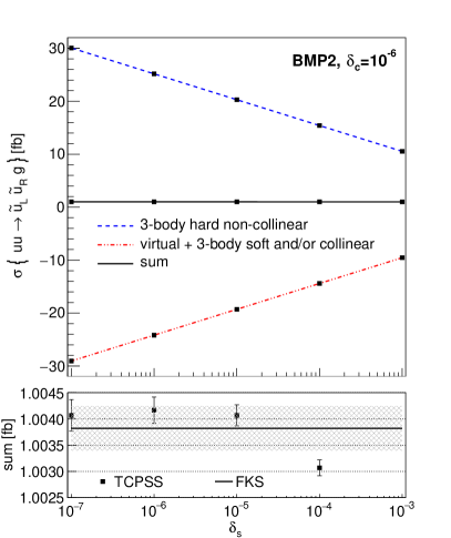
(a)

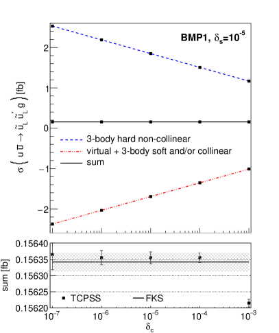
(b)

Figure 5: Proof of cut parameter cancellation for the two selected subprocesses
$uu\to\tilde{u}_{L}\tilde{u}_{R}g$ and $u\bar{u}\to\tilde{u}_{L}\tilde{u}_{L}^{\dagger}g$. Given errors correspond to 68% CL.

The comparison with the FKS subtraction reveals that a relative accuracy of $10^{-4}$ requires the cut parameters $\delta_{s}=10^{-5}$ and $\delta_{c}=10^{-6}$, which is what we use in our numerical analyses.

As the TCPSS method relies on a partial cancellation of two large contributions at the level of an integrated cross sections, it is inherently slower than local subtraction schemes like FKS. For the case at hand, this means an order of magnitude slow down for the same final precision. This directly translates into an order of magnitude speed difference between the standalone C++ code and the MG5aMC@NLO as for the standalone calculation most time is spend evaluating the $2\to 3$ hard non-collinear part.

5.4 Treatment of resonances in real emission diagrams using diagram removal

Figure 6: Example of real emission Feynman diagrams with s-channel gluinos for both final states: $gu\to\tilde{u}_{L}\tilde{u}^{\dagger}_{L}u$ and $gu\to\tilde{u}_{L}\tilde{u}_{R}\bar{u}$.

Certain real corrections to the considered processes may contain Feynman diagrams with an intermediate massive state in an s-channel. As examples consider diagrams shown in figure 6 where an intermediate s-channel gluino appears. From a practical point of view, the region of phase space where the gluino goes on-shell should rather be classified as a Born-level gluino-squark production followed by a subsequent decay of the gluino. This feature is not exclusive to BSM models as a similar issue appears in the case of the real corrections to the SM $tW$ production (see e.g. ref. Frixione:2008yi ), which contain resonant contributions from the top pair production.

A popular way of dealing with this problem is the diagram removal technique. In this approach one either completely discards all resonant diagrams at the level of the amplitude or their square at the level of the squared matrix element. In this work we employ the first of those solutions. This version of the DR approach is also the default way of dealing with resonant divergences when using MadFKS in MG5aMC@NLO.

The removal of a subset of Feynman diagrams in general violates gauge invariance and care has to be taken to ensure that the effect is numerically small. For the case of the MSSM this has been studied in depth in refs. Gavin:2013kga ; Gavin:2014yga (see also refs. Hollik:2012rc ; GoncalvesNetto:2012yt for other implementations). Also, it requires a careful choice of a gauge not to spoil the factorisation of collinear singularities.

To understand this last point, consider the gluon splitting $g(p_{1})\to\bar{q}^{*}(p_{1}-p_{5})q(p_{5})$ connected to some bigger amplitude through $\bar{q}$. We use the $*$-symbol to emphasise that $\bar{q}$ is in general not on-shell. The final state quark momentum $p_{5}$ can be parametrised through Sudakov decomposition as

$$p_{5}^{\mu}=(1-z)p_{1}^{\mu}-\frac{p_{5,\perp}^{2}}{1-z}\frac{n^{\mu}}{2p_{1}\cdot n}-p_{5,\perp}^{\mu},$$ (54)

where $n^{\mu}$ is a reference null vector, $1-z$ is the fraction of gluon energy carried by the quark, and $p_{5,\perp}\cdot p_{1}=p_{5,\perp}\cdot n=0$. In the limit of $p_{5,\perp}\to 0$ the vectors $p_{1}$ and $p_{5}$ become spatially parallel and diagrams with this splitting develop a $(p_{1}-p_{5})^{-2}=(1-z)/p_{5,\perp}^{2}$ singularity. Due to the helicity conservation, physical gluons cannot decay to a pair of on-shell quarks. Therefore, in the physical gauge the matrix element will always have additional power of $p_{5,\perp}$ in the numerator. As the one particle phase space for radiation of $q$ is given by $d\Phi_{1}\sim dp_{5,\perp}^{2}$, the collinear singularities of the interference terms are integrable since those terms scale as $dp_{5,\perp}^{2}/p_{5,\perp}$. This is no longer true in an unphysical gauge, where longitudinally polarised gluons might appear. For the full amplitude with a $ug$ initial state, which is gauge invariant, longitudinal states decouple through a Ward identity as no triple gluon vertices appear. This is no longer true after the removal of resonant diagrams, though.

We therefore calculate the real emission matrix elements in the light cone gauge. A convenient choice of the gauge-fixing vector $\eta$ is the momentum of the other incoming parton $p_{2}$. This choice allows to avoid spurious divergences present in the polarisation sum as $p_{1}\cdot p_{2}=\hat{s}/2$. To study the numerical impact of this gauge choice we consider two families of gauge vectors (assuming the momenta $p_{1,2}$ oriented in the $\pm$z-direction)

$$\eta_{-}\equiv (\sqrt{1+\delta^{2}},0,\delta,-1),$$ (55)

$$\eta_{+}\equiv (\sqrt{1+\delta^{2}},0,\delta,+1).$$ (56)

For $\delta=0$ the $\eta_{-}$ choice is equivalent to the choice of $\eta=p_{2}$, while the $\eta_{+}$ choice is singular as $p_{1}\cdot\eta_{+}=0$. In the limit of $\delta\gg 1$ results of both gauge choice converge as $\eta_{+}\simeq\eta_{-}$. Both of these features are clearly seen in figure 7, where we plot the cross sections for $gq\to\tilde{u}_{L}\tilde{u}_{L}^{\dagger}q$ with $q=u,\bar{u}$ (7a) and $gu\to\tilde{u}_{L}\tilde{u}_{R}\bar{u}$ (7b) in function of the $\delta$ parameter for BMP2. For $gu\to\tilde{u}_{L}\tilde{u}_{R}\bar{u}$ the gauge dependence is enhanced since resonant diagrams were giving a substantial contribution to this amplitude.

(a)

(b)

Figure 7: Gauge dependence of a diagram removed $gq\to\tilde{u}_{L}\tilde{u}_{L}^{\dagger}q$ with $q=u,\bar{u}$ (a) and $gu\to\tilde{u}_{L}\tilde{u}_{R}\bar{u}$ (b) matrix elements. See eqs. (55) and (56) for the definition of $\eta_{-}$ and $\eta_{+}$ gauges.

We point out, that keeping the choice of the non-singular gauge $\eta_{-}$, the DR subtracted processes give per mille level contribution to the total cross section. Hence, for all intents and purposes, the gauge dependence is not a problem and for studies in the following sections we use the customary choice of $\eta=p_{2}$.

6 Results

When the virtual corrections of section 4 are combined with the real contributions from section 5 all IR divergences cancel as expected and we are able to calculate the NLO SUSY-QCD cross section for $\tilde{q}\tilde{q}$ and $\tilde{q}\tilde{q}^{\dagger}$ production in the MRSSM. In this section we first point out and explain the consequences of R-symmetry on NLO cross sections in supersymmetric QCD before exhibiting the results of our calculations for $\tilde{q}\tilde{q}$ and $\tilde{q}\tilde{q}^{\dagger}$ production. We conclude with remarks on the scale dependence and uncertainties of the computed observables.

A useful quantity which helps to understand these different aspects is the K-factor. We define a K-factor $K$ as ratio of NLO over LO total cross section following ref. Beenakker:1996ch :

$$K(\text{NLO/LO})=\frac{\sigma_{\text{NLO}}}{\sigma_{\text{LO}}(NLO/LOPDF)}\,,$$ (57)

where $\sigma_{\text{NLO}}$ is calculate using NLO PDFs and $\sigma_{\text{LO}}$ using NLO or LO PDFs, depending on the argument. If no argument is given we use LO PDF sets as default case for $\sigma_{\text{LO}}$. The K-factor depends on the process, masses of the fields in the model, and the centre-of-mass energy, as well as the choice of renormalisation and factorisation scale. In the following, we set $\sqrt{S}=13\,\mathrm{TeV}$ and $\mu_{R}=\mu_{F}=\frac{m_{1}+m_{2}}{2}$, where $m_{i}$ are the final state’s particle masses. For a consistent definition we identify the values of the Dirac gluino mass in the MRSSM with the Majorana gluino mass in the MSSM, the values of the squark masses in both models, as well as neglecting left-right squark mixing in the MSSM. In the MRSSM the K-factor has an additional dependency on the sgluon mass parameter. To fix all remaining SM parameters, we set the top quark mass to $m_{t}=172$ GeV and take the strong coupling constant $\alpha^{\overline{\text{MS}}}_{s}(m_{Z})$ from the used PDF set.

6.1 Effects of R-symmetry

The results of R-symmetry at NLO may be pinned down to two features: the presence of a Dirac instead of Majorana gluino and the existence of sgluons. The conservation of R-charge, already discussed at LO in section 3, also needs to be commented on when comparing K-factors to the MSSM. The effect of R-symmetry is however only present in the virtual corrections, i.e. the real corrections do not differ in the MSSM and MRSSM.

The effects discussed in the following comprise the unique features of MRSSM neglected in the study of ref. Kribs:2012gx by only taking MSSM NLO K-factors into account.

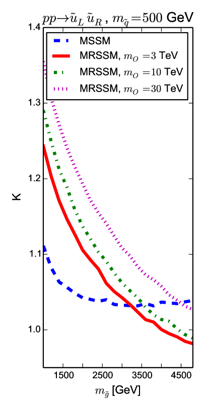
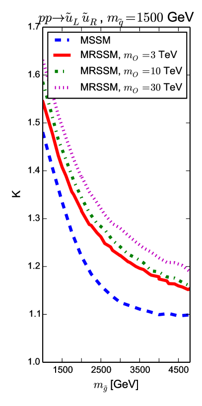
Figure 8: Comparison of K-factor dependence on the gluino mass between the MSSM and the MRSSM at different octet masses shown for two different squark masses.

Figure 9: Dependence of the K-factor on the sgluon mass for $\tilde{q}\tilde{q}$ and $\tilde{q}\tilde{q}^{\dagger}$ production in the MRSSM.

6.1.1 Dirac nature of the gluino

In the presentation of renormalisation constants in section 4.1, we already saw ramifications of the Dirac gluino whose components couple differently. Now, we study the effect of replacing the Majorana with a Dirac gluino in a physical process.

To this end, consider diagram 1a) and 1b) (referring to the first diagram of category a) and b), respectively) of Figure 4. The former contributes in both models, whereas the latter is only non-zero in the MSSM, since the gluino undergoes a chirality flip to its non-coupling right-handed component. Taking only objects with spinor indices into account these diagrams evaluate to

$$\mathcal{M}_{1a)} \propto\bar{v}(p_{2})P_{R}(\not{t}+m_{\tilde{g}})P_{L}\not{q}P_{R}(\not{t}+m_{\tilde{g}})P_{L}u(p_{1})=\bar{v}(p_{2})\not{t}\not{q}\not{t}P_{L}u(p_{1}),$$ (58)

$$\mathcal{M}_{1b)} \propto\bar{v}(p_{2})P_{R}(\not{t}+m_{\tilde{g}})P_{R}\not{q}P_{L}(\not{t}+m_{\tilde{g}})P_{L}u(p_{1})=m_{\tilde{g}}^{2}\bar{v}(p_{2})\not{q}P_{L}u(p_{1}).$$ (59)

Here $q^{\mu}$ is the quark’s loop momentum and $m_{\tilde{g}}$ is the Majorana gluino mass of the MSSM, which is zero in the MRSSM. Hence diagram 1a) is the same in both models, while diagram 1b) vanishes in the MRSSM. Alternatively, diagram 1b) can also be understood to be zero in the MRSSM as R-charge is not conserved at all vertices of the diagram as the R-charge of the gluino flows in the opposite direction than the one of the squark appearing in its self energy insertion.

On similar grounds we are able to understand why diagram 2b) in figure 4 does not contribute in the MRSSM. Its matrix element has the following proportionality

$$\mathcal{M}_{2b)}\propto\bar{v}P_{R}(\not{t}+m_{\tilde{g}})P_{R}\not{q}P_{L}(\not{q}+\not{p}_{3}+m_{\tilde{g}})P_{L}u=m_{\tilde{g}}^{2}\bar{v}\not{q}P_{L}u$$ (60)

in the MSSM and is therefore zero in the MRSSM. Note that its analogue, depicted as diagram 2a) in figure 4 is proportional to the $u$-quark mass and therefore zero in both models. Diagram 3b) of figure 4 appears only for $\tilde{q}\tilde{q}^{\dagger}$ production and is proportional to the Majorana mass of the MSSM squared for the same reasoning as discussed before.

The number of diagrams affected by the difference between Dirac and Majorana mass is only a subset of all contributing virtual graphs. Therefore, the effect is most apparent when we use the dependency on the gluino mass and make it large compared to all other appearing scales. This can be seen when comparing the plots of figure 9. On the right plot, where the mass scales are not too different from each other, the MRSSM and MSSM line have a similar dependency on the gluino mass, where the magnitude of the K-factor is affected by the sgluon mass as described below. If, however, the squark mass is reduced, the behaviour changes drastically for large gluino masses. Then, the additional contributions in the MSSM lead to a K-factor rising with gluino mass, instead of falling like in the MRSSM.

6.1.2 Sgluon non-decoupling effects

The sgluon necessarily appears in the MRSSM as the scalar superpartner of the additional component of the Dirac gluino. The sgluon affects the MRSSM prediction in several ways. Obviously, it enters the virtual corrections as new matter content, contributing to the $\beta$ function of the strong coupling such that it becomes zero at one-loop level. Furthermore, the mass of the pseudo-scalar (scalar) component is determined (mostly) by the SUSY breaking mass parameter $m^{2}_{O}$, which is independent of the gluino mass as can be seen in eq. (4). It is therefore possible that the sgluon can be much heavier than the gluino and not be directly observable at the LHC. Still, effects of the sgluon could be experimentally accessible, even if superheavy, as a mass splitting between superpartners in a SUSY multiplet leads to non-decoupling, so called super-oblique, contributions Cheng:1997sq .

Super-oblique effects lead to a physical difference between the gauge coupling $g_{s}$ and the gaugino coupling $\hat{g}_{s}$ at loop level. It can be understood in the context of an effective field theory (EFT) where the sgluon is integrated out. In the EFT, the sgluon decouples from the gauge boson and gaugino self-energies (first two diagrams in category c) of figure 3) which changes the corresponding field renormalisation constants and therefore induces a change in the corresponding couplings $g_{s}$ and $\hat{g}_{s}$. This produces a one-loop difference of

$$\hat{g}_{s}-g_{s}=\frac{\alpha_{s}}{8\pi}\left(\log\frac{m_{O_{s}}^{2}}{m_{\tilde{g}}^{2}}+\log\frac{m_{O_{p}}^{2}}{m_{\tilde{g}}^{2}}\right)$$ (61)

in the theory without sgluon. The production of $\tilde{u}_{L}\tilde{u}_{R}$ at the LHC is mediated by the gluino alone at tree level. Therefore, the super-oblique contribution from the sgluons can be written as product of the total tree-level cross section and the difference given by eq. (61) such that

$$\sigma^{\text{super-oblique part}}_{pp\to\tilde{u}_{L}\tilde{u}_{R}}=\frac{\alpha_{s}}{2\pi}\left(\log\frac{m_{O_{s}}^{2}}{m_{\tilde{g}}^{2}}+\log\frac{m_{O_{p}}^{2}}{m_{\tilde{g}}^{2}}\right)\sigma^{\text{LO}}_{pp\to\tilde{u}_{L}\tilde{u}_{R}}\,.$$ (62)

The result for $\tilde{q}\tilde{q}^{\dagger}$ production is more complicated as the gluino only appears in a subset of the diagrams at tree level. Hence, the non-decoupling correction to the cross section affects only a part of the contributions, not allowing for a simple factorisation as before.

The sgluon can influence the prediction of the MRSSM in another way, namely via the sgluon-squark-antisquark vertex induced by the gluino mass parameter, see of the Feynman rules in appendix A. This leads to additional terms in the renormalisation constants, stemming from the third Feynman diagram in category c) of figure 3, as well as additional virtual corrections to the processes, see the last three diagrams of category c) in figure 4. We have checked that these contributions are small compared to the super-oblique corrections.

In figure 9, the effect of super-oblique corrections is visible when comparing lines with different sgluon masses. As expected, their spacing follows the logarithmic dependency described by eq. (62) for small gluino masses. When comparing the lines for $m_{O}=3\,\mathrm{TeV}$ and $m_{O}=10\,\mathrm{TeV}$ at large gluino masses it can be seen that the differences between the K-factors is reduced, as the assumption that sgluons can be integrated out is not valid. Then, also ratios of the sgluon masses to the Mandelstam variables become relevant.

Figure 9 shows the effect at very large sgluon masses for both $\tilde{q}\tilde{q}$ as well as $\tilde{q}\tilde{q}^{\dagger}$ production. For both processes we find the logarithmic enhancement for large sgluon masses, more prominently for $\tilde{q}\tilde{q}$ production as discussed before. Super-oblique corrections lead to a difference in the K-factors of roughly twenty (five) per cent when the sgluon masses changes by two orders of magnitude for $\tilde{q}\tilde{q}$ ($\tilde{q}\tilde{q}^{\dagger}$) production.

6.1.3 R-charge forbidden processes

For $\tilde{q}\tilde{q}$ production we have seen that in the MRSSM only the production of left- and right-handed squarks together is allowed, while the production of squarks with the same “chirality” is forbidden by R-charge conservation. This is relevant when comparing the MRSSM K-factor for e.g. $pp\to\tilde{u}_{L}\tilde{u}_{R}$ to the MSSM: should we compare it to the MSSM K-factor for $pp\to\tilde{u}_{L}\tilde{u}_{R}$, or to the MSSM K-factor for total squark production, $pp\to\tilde{u}_{L}\tilde{u}_{R},\tilde{u}_{L}\tilde{u}_{L},\tilde{u}_{R}\tilde{u}_{R}$? The second K-factor is commonly available via tools like Prospino Beenakker:1996ed or NNLLfast Beenakker:2016lwe and used by the experimental collaborations for MSSM analyses. The first, however, allows a more direct comparison between the models.

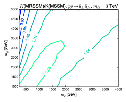
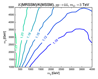
Figure 10: Shown is the ratio of MRSSM over MSSM K-factors for $\tilde{q}\tilde{q}$ production for $m_{O}=3$ TeV. In the MSSM, only left-right $\tilde{q}\tilde{q}$ production (left) or all channels (right) are included.

This point is depicted in figure 10. The left-hand plot compares the ratios of K-factors (MRSSM over MSSM) for the same process, i.e. $pp\to\tilde{u}_{L}\tilde{u}_{R}$ which is equivalent to the ratio of NLO cross sections. It therefore allows to view the effects of the sgluons and Dirac-gluinos at NLO. On the other hand, the right-hand plot contrasts the K-factors for full $u$-squark production, i.e. $K(\mathrm{MSSM})$ is the usual K-factor including $\tilde{u}_{L}\tilde{u}_{L}$ and $\tilde{u}_{R}\tilde{u}_{R}$ production. Thus, this plot does not solely illustrate NLO effects but also the conservation of R-charge, already present at LO.

On the left of figure 10 it can be seen that the sgluon and Dirac mass effects can lead to a difference of the K-factor of five to eight per cent between the MRSSM and the MSSM when considering only the $\tilde{u}_{L}\tilde{u}_{R}$ production. The ratio is smaller than one for $m_{\tilde{q}}\ll m_{\tilde{g}}$ and larger than one in the other parts of parameter space with the maximum at the ratio of $m_{\tilde{g}}/m_{\tilde{q}}=2$. However, when the K-factor for the summed production in the MSSM is used the ratio deviates significantly from one. Using the usual, summed K-factor of the MSSM to estimate NLO MRSSM cross sections from LO ones would consequently lead to a systematic underestimate between $10\%$ and $23\%$.

6.2 Squark production at NLO

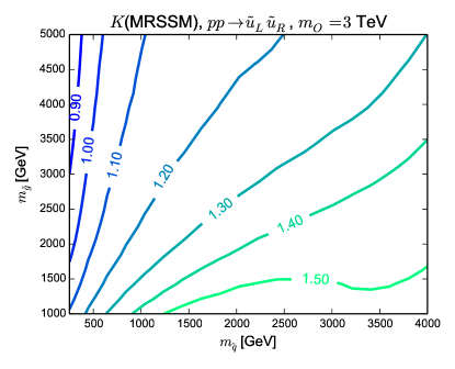
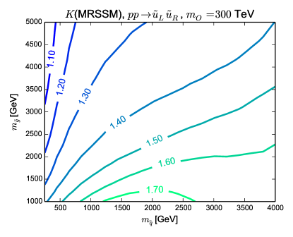
Figure 11: Shown are the MRSSM K-factors for $\tilde{u}_{L}\tilde{u}_{R}$ production for two different octet masses.

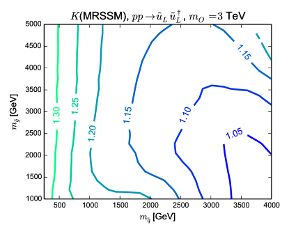
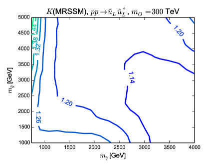
Figure 12: As figure 11 for $\tilde{u}_{L}\tilde{u}_{L}^{\dagger}$ production.

We have described the qualitative differences of the NLO corrections between the MRSSM and MSSM in the previous section, especially highlighting the role of the Dirac gluino mass and the appearance of the sgluon. In the following, we give an overview of the quantitative features of the corrections in the MRSSM analysing the variation of the K-factor. Figures 11 and 12 summarise the dependency of the K-factor on the different masses of the strong sector for $\tilde{q}\tilde{q}$ and $\tilde{q}\tilde{q}^{\dagger}$ production, respectively. The left (right) plot of each figure is given for a sgluon mass of 3 TeV (300 TeV) and shows the K-factor depending on the Dirac gluino and common squark masses.

As discussed before, the change of the sgluon mass from 3 to 300 TeV leads to a global enhancement of the K-factor of around twenty per cent in the whole parameter plane for $\tilde{q}\tilde{q}$ production which originates from the super-oblique corrections. The increase for the $\tilde{q}\tilde{q}^{\dagger}$ production is reduced to about five per cent as only part of the contributions receive the relevant corrections.

For $\tilde{q}\tilde{q}$ production, the total NLO contributions can decrease the LO cross section by $10\%$ and can increase them by more than $50\%$ of the LO prediction assuming sgluons are close in mass to gluino and squarks. The relative size of the corrections falls with rising gluino mass while increasing squark masses lead to an enhancement. This feature is already present in the MSSM Beenakker:1996ch and not influenced by the Dirac nature of the gluino or the presence of the sgluon. In the scenario of interest, with a heavy Dirac gluino and rather light squarks, the size of NLO corrections is reduced compared to the remainder of the parameter space.

The K-factors for $\tilde{q}\tilde{q}^{\dagger}$ production are in general smaller than for $\tilde{q}\tilde{q}$ production. They yield up to $30\%$ corrections to the LO production cross section. The corrections are largest for small squark and gluino masses. For small squark masses, the gluino mass does not influence the K-factor significantly. In this region pure QCD corrections are dominant and only with a large sgluon mass do the effects described in section 6.1.2 become important. The K-factor is smallest for large squark masses and increases in this parameter region with the gluino mass.

6.3 Full results including uncertainties

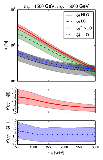
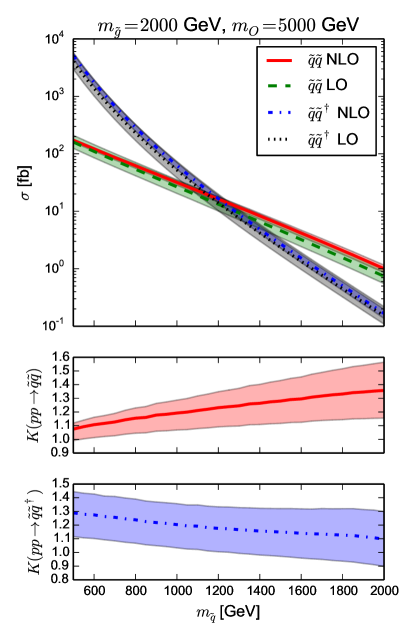
Figure 13: Total LO and NLO cross section as function of the gluino (left) and common squark mass (right) with uncertainties. Shown are $\tilde{q}\tilde{q}$ and $\tilde{q}\tilde{q}^{\dagger}$ production summed over all possible flavour combinations as well as the corresponding K-factors. The bands give the $68\%$ CL combined scale and pdf uncertainties as described in the text.

We illustrate in figure 13 the summarising results of our study of the NLO SUSY-QCD corrections for the production of squarks in the MRSSM. The plots show LO and NLO cross sections for $\tilde{q}\tilde{q}$ and $\tilde{q}\tilde{q}^{\dagger}$ production and their dependence on the squark and gluino mass as well as the corresponding K-factors. The uncertainty bands are calculated by summing the uncertainty of the scale dependence and the PDF uncertainty in quadrature. A detailed study of both sources of uncertainty is described below.

As we have seen before and has been known from the MSSM, the plots highlight that NLO QCD corrections are in general large and usually positive. Comparing the LO and NLO predictions including their respective $68\%$ CL uncertainty bands we see that the bands overlap for most of the parameter space and the NLO corrections show no unexpected behaviour.

Comparing the cross sections for the MRSSM calculated with NLO precision to the ones of the MSSM, the distinctions between both models are similar to the ones already discussed at tree level in section 3. These differences stem from the conservation of R-charge in the MRSSM so that only different (same) “chiralities” of squarks can be produced in $\tilde{q}\tilde{q}$ ($\tilde{q}\tilde{q}^{\dagger}$) production as has been discussed in detail in section 6.1.3.

Effects from the existence of sgluons becomes relevant only for sgluon masses above hundreds of TeVs. The Dirac nature of the gluino in the virtual contributions is of influence in the region of light squarks and large gluino mass but does not alter the behaviour of the cross section significantly compared to the tree-level differences.

The relative uncertainties of the cross sections are reduced from $50\%$ or more to below $20\%$ when going to NLO. The dominating uncertainty component comes from the scale variation. Therefore, a further reduction of the uncertainties would require going to next-to NLO and/or including effects from the resummation of threshold corrections as has been done for the MSSM predictions Beenakker:2011fu ; Falgari:2012hx .

		$\sigma_{\text{LO}}(\text{LO PDF})[\text{fb}]$	$\sigma_{\text{LO}}(\text{NLO PDF})[\text{fb}]$	$K(\text{LO})$	$K(\text{NLO})$
BM1	$\tilde{q}\tilde{q}$	$13.1$	$11.2$	$1.46$	$1.75$
	$\tilde{q}\tilde{q}^{\dagger}$	$3.75$	$2.72$	$1.18$	$1.62$
BM2	$\tilde{q}\tilde{q}$	$4.61$	$3.92$	$1.28$	$1.51$
	$\tilde{q}\tilde{q}^{\dagger}$	$2.36$	$1.78$	$1.15$	$1.52$
BM3	$\tilde{q}\tilde{q}$	$160$	$146$	$1.08$	$1.18$
	$\tilde{q}\tilde{q}^{\dagger}$	$3990$	$3470$	$1.29$	$1.48$

Table 3: LO cross section and corresponding K factors for the benchmark points of table 2 using PDF sets of LO and NLO.

We show in figure 13 the K-factor defined in equation (57) using the LO PDF sets for the LO cross section. Alternatively, it is also possible to use the NLO PDF sets for both, NLO and LO cross section. The difference is studied based on table 3, where the LO cross sections and NLO K factors using either LO or NLO PDF sets are given for the benchmark points of table 2 and both squark production processes of this paper.

In general, using the NLO PDF sets for the LO cross section leads to an enhancement of the K factor (reduction of the LO cross section) arising from the difference in the strong coupling constant between the two sets. (Here, with $\alpha^{\overline{\text{MS}}}_{s}(m_{Z})=0.135$ for $\mathtt{MMHT2014LO}$, $\alpha^{\overline{\text{MS}}}_{s}(m_{Z})=0.120$ for MMHT2014nlo68cl.) This can be seen when comparing the changes in the K-factors between BM2 and BM3. They differ by the choice of squark mass which is used as renormalisation and factorisation scale relevant for the extraction of the correct $\alpha^{\overline{\text{MS}}}_{s}(\mu_{R})$. For BM2 with a larger squark mass the difference in K-factors is enhanced compared to BM3.

Additional effects due to difference in the PDF fits for quark and gluon are also present. This leads to an enhancement of $\tilde{q}\tilde{q}^{\dagger}$ compared to the $\tilde{q}\tilde{q}$ production with rising squark mass.

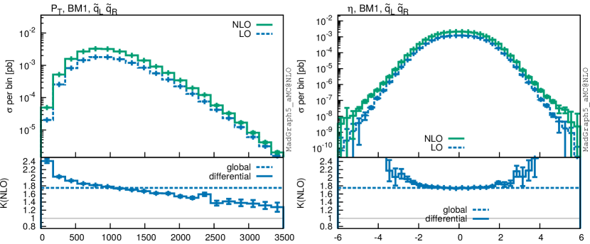
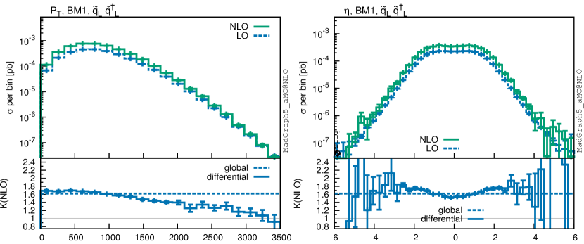
Figure 14: Differential cross section of $\tilde{q}\tilde{q}$ and $\tilde{q}\tilde{q}^{\dagger}$ production as function of the transversal momentum $p_{T}$ or the pseudo-rapidity $\eta$ for BM1. The integration error is given.

For the results of this work we assume that all squark masses are at the same value. We also investigated the scenario, where the constraint of equal squark masses was dropped. We checked that the quantum corrections are well behaved in this case. The phenomenological effects of such a scenario, especially for final state squarks of different masses, will be studied in forthcoming work. In the following, we describe in detail the scale and PDF uncertainties as well as differential distributions of the NLO SUSY-QCD corrections.

6.3.1 (Fixed) Renormalisation and factorisation scale dependency

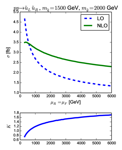
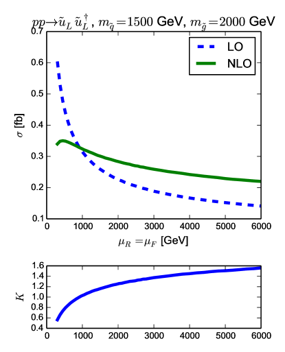
Figure 15: Scale dependency of the cross section for $\tilde{u}_{L}\tilde{u}_{R}$ (left) and $\tilde{u}_{L}\tilde{u}_{L}^{\dagger}$ (right) production in the MRSSM at LO and NLO.

A major motivation to calculate perturbative corrections to the prediction of a cross section is the reduction of the theoretical uncertainty. One way of quantifying this is the variation of renormalisation and factorisation scale.

Figure 15 shows the variation of scales for $\tilde{u}_{L}\tilde{u}_{R}$ and $\tilde{u}_{L}\tilde{u}_{L}^{\dagger}$ production. To achieve a qualitative understanding renormalisation and factorisation scale are set equal and varied together. The prediction of the cross section at LO changes by more than $50\%$ when the scale is varied from the reference value at $\mu_{R}=\mu_{F}=m_{\tilde{q}}$ by a factor of two. This variation uncertainty is reduced to below $20\%$ when taking NLO corrections into account. This difference in the scale dependency also leads to a strong dependence of the K-factor, as shown in the lower plot, which can become smaller than one for a certain choice.

The commonly accepted range for the variation of the scales is $[\mu_{R,F}/2,2\cdot\mu_{R,F}]$ where, for the most conservative approach, both scales are varied independently and one takes the envelope of those nine values as final estimate. This is the procedure we use to estimate the scale uncertainty in figure 13.

6.3.2 PDF uncertainty

	MMHT2014nlo68cl	MMHT2014nlo68clas118	CT14nlo	NNPDF30_nlo_as_0118
BM1	$9.94^{+3.5\%}_{-3.4\%}$	$9.86^{+3.4\%}_{-3.3\%}$	$10.1^{+3.3\%}_{-3.4\%}$	$10.1^{+3.2\%}_{-3.2\%}$
BM2	$3.01^{+3.5\%}_{-3.4\%}$	$3.00^{+3.4\%}_{-3.3\%}$	$3.08^{+3.4\%}_{-3.6\%}$	$3.04^{+3.3\%}_{-3.3\%}$
BM3	$64.0^{+3.0\%}_{-3.0\%}$	$62.4^{+3.1\%}_{-2.9\%}$	$65.0^{+2.6\%}_{-2.4\%}$	$64.0^{+2.4\%}_{-2.4\%}$

Table 4: Cross section (in fb) of $\tilde{u}_{L}\tilde{u}_{R}$ production for the benchmark points of table 2 using different PDF sets. The first set is the standard NLO PDF of this paper. The other columns compare different PDF sets at $\alpha_{s}(m_{Z})=0.118$. The factorisation and renormalisation scale are set to the common squark mass. All uncertainties are given at $68\%$ CL. For this the uncertainties of the CT14 set have been rescaled by $1.642$ as the default is given at $90\%$ CL. Butterworth:2015oua

	MMHT2014nlo68cl	MMHT2014nlo68clas118	CT14nlo	NNPDF30_nlo_as_0118
BM1	$0.512^{+7.6\%}_{-5.4\%}$	$0.503^{+7.5\%}_{-4.9\%}$	$0.503^{+12.9\%}_{-11.6\%}$	$0.588^{+9.7\%}_{-9.7\%}$
BM2	$0.301^{+8.1\%}_{-5.7\%}$	$0.294^{+7.7\%}_{-5.0\%}$	$0.300^{+14.8\%}_{-11.1\%}$	$0.335^{+9.9\%}_{-9.9\%}$
BM3	$502^{+3.8\%}_{-3.7\%}$	$509^{+3.9\%}_{-3.4\%}$	$512^{+6.7\%}_{-5.4\%}$	$533^{+3.4\%}_{-3.4\%}$

Table 5: Cross section (in fb) of $\tilde{u}_{L}\tilde{u}_{L}^{\dagger}$ production for the benchmark points of table 2 using different PDF sets. All details as for table 4.

Another main source of uncertainty for the cross section prediction at a hadron collider comes from the use of PDFs as they can not be calculated from first principles but need to be extracted from data. Details on this and the application at LHC Run II can be found in ref. Butterworth:2015oua . Here, we only aim to achieve a basic understanding of the relevant PDF uncertainties. For this we compare the cross section for our three BMPs defined in table 2 and both processes calculated with our default set, MMHT2014nlo68cl, against one of the same group with a different fit value for $\alpha_{s}(m_{Z})$, MMHT2014nlo68clas118. Additionally, we compare to cross sections calculated using the CT14 Dulat:2015mca and NNPDF3.0 Ball:2014uwa PDF set with $\alpha_{s}(m_{Z})=0.118$. They are summarised in the tables 4 and 5 .

The difference of the result for the MMHT2014nlo68cl and MMHT2014nlo68clas118 sets stems only from the strong coupling constant, $\alpha_{s}(m_{Z})=0.120$ and $\alpha_{s}(m_{Z})=0.118$ respectively, and gives an estimate for the uncertainty coming from this input parameter. For the considered points the uncertainty is at most a few per cent. The different PDF sets for $\alpha_{s}(m_{Z})=0.118$ all agree within their uncertainty as expected from the comparison done in ref. Butterworth:2015oua . The uncertainty of the individual sets is below five per cent for $\tilde{q}\tilde{q}$ production. This is understandable as for this mainly the up quark PDF is relevant which is rather well determined, see figure 6 of ref. Butterworth:2015oua . The PDF uncertainty for $\tilde{q}\tilde{q}^{\dagger}$ production on the other hand is increased and can reach $10\%$ to $15\%$ depending on the PDF set. This originates from the appearance of initial gluons and antiquarks as in this case the PDFs are not as well known, see figure 5 of ref. Butterworth:2015oua .

As the study of PDF uncertainties is not in the focus of this work, the PDF uncertainty in figure 13 contains only the uncertainty of the MMHT2014nlo68cl set.

6.3.3 Dynamical scales and differential distributions

The main concern of this work was to perform the calculation of NLO corrections for the MRSSM and highlight the physical differences to the MSSM. We addressed it by focusing on global K-factors and using fixed renormalisation and factorisation scales. Here we give a brief comment on going beyond that. The MG5aMC@NLO framework allows in principle to use dynamical renormalisation and factorisation scales (as opposed to fixed ones studied in section 6.3.1) and to study differential distributions at the NLO. We have verified that these components work as expected. The global K-factors vary by less than five per cent when choosing between a fixed (like the common squark mass) and a dynamical (like the total transverse mass in an event) scale. As there is no physically preferred scheme we follow the works on the MSSM Gavin:2013kga ; Gavin:2014yga ; Hollik:2012rc ; GoncalvesNetto:2012yt and use fixed renormalisation and factorisation scales.

In figure 14, we show sample differential distributions in the transversal momentum $p_{T}$ and the pseudo-rapidity $\eta$ for the benchmark point BM1. The top row shows it for $\tilde{q}\tilde{q}$ while in the bottom $\tilde{q}\tilde{q}^{\dagger}$ production is given. The K-factor can actually vary substantially over the different kinematic regions changing by 50 per cent or more. Still, for the regions containing the bulk of the contributions ($500\,\mathrm{GeV}<p_{T}<1000\,\mathrm{GeV}$ and $-2<\eta<2$) the global K-factor is a good approximation.

7 Conclusions

The Minimal R-symmetric Supersymmetric Standard Model is a well-motivated, viable model. It provides a realisation of SUSY distinct from the familiar MSSM with a significantly modified coloured sector: The gluino carries R-charge and is of Dirac instead of Majorana nature, and there are scalar and pseudoscalar colour octets, the sgluons. Left- and right-handed squarks carry opposite R-charge. In a motivated region of parameter space, the squark masses are around the TeV-scale while the gluino and sgluons are somewhat heavier.

Here we have presented an analysis of squark production at the LHC in the MRSSM taking into account NLO corrections of the entire strongly interacting sector. Both the tree-level results and the NLO corrections show important features and differences to the MSSM:

• In the MRSSM only opposite-chirality squarks can be pair-produced, i.e. $\tilde{q}_{L}\tilde{q}_{R}$ production is allowed, while $\tilde{q}_{L}\tilde{q}_{L}$ and $\tilde{q}_{R}\tilde{q}_{R}$ are forbidden by R-charge conservation. For squark-antisquark production, the converse statement is true. Owing to this, the overall squark production rate in the MRSSM is lower than in the MSSM.

• When comparing K-factors between the two models one has to be careful to distinguish in the MSSM between the K-factor for total squark production and the K-factor specific for e.g. $\tilde{q}_{L}\tilde{q}_{R}$ production. The first is the one usually quoted; it differs from the MRSSM counterpart by $10$ to $20\%$. The second is usually not quoted in the MSSM, but it is more directly comparable between the two models.

• Even the comparison between $\tilde{q}_{L}\tilde{q}_{R}$ production in the MRSSM and MSSM reveals several differences between the two models. The MRSSM Dirac gluino enters the loop corrections differently from the MSSM Majorana gluino, and large sgluon masses lead to non-decoupling, logarithmic enhancements of the NLO corrections. To a lesser degree, these effects also lead to differences in the $\tilde{q}\tilde{q}^{\dagger}$ production.

Our study also has technical aspects. During the last decade several efforts lead to fast and automatised ways to evaluate SM processes at NLO and beyond. In recent years, there has been a push to expand this also to BSM models. Usually, this added capability is tested in the context of well-known and understood models like the THDM or the MSSM. In this paper we were able to achieve full agreement between a calculation based on a subset of publicly available tools and an independent calculation for NLO QCD corrections of the MRSSM. The latter calculation uses the techniques, described as method 1 in this paper and results will be available via the soon to be published RSymSQCD code our_code . The MRSSM provides a valuable test of the implemented mechanisms as it contains unique features complementary to the previous test cases. It therefore shows how far the latest available machinery can be pushed. It also illustrates the possibility mentioned in ref. Signer:2008va ; Gnendiger:2017pys , to compute QCD corrections to SUSY processes in different renormalisation schemes.

The results obtained here are not specific for the MRSSM but can be applied more generally also to other models with R-symmetry and a difference in R-charge assignment. This only requires that the particle content under consideration is the same and all the SUSY QCD vertices given in the appendix are present.

It will be now of high interest to identify the allowed squark mass range in the MRSSM in the light of current LHC data. In line with simplified studies Kribs:2012gx ; Kribs:2013oda we expect that significantly lighter squarks are allowed in the MRSSM, thanks to the fewer allowed production channels. On the other hand, our NLO results show that the assumption that the K-factors in the MSSM and MRSSM are equal is not correct. The MRSSM K-factors are higher and dependent on the hierarchies between squark, gluino and sgluon masses and should be taken into account to obtain valid limits.

Appendix A Feynman rules

In SUSY models, it is often not possible to define a consistent, conserved fermion number. To compute Feynman diagrams in an unambiguous way, a fermion flow can be introduced Denner:1992vza ; Denner:1992me , which does in general not agree with the flow of fermion number.

Even though there are no Majorana particles in the MRSSM, it is useful to adapt this procedure. The reason for this is the existence of fermion number violating processes like $qq\to\tilde{q}\tilde{q}$, which results in a clash of arrows in the associated Feynman diagrams.

In the following we list Feynman rules for the MRSSM which are new or different to the ones in the MSSM. We labelled the lines with the corresponding quantum field operators of the respective Lagrangian term (thus this labeling does not coincide with the labels of external particles in section 3 and 4). The fermion flow on vertices is always directed from an unbarred to a barred spinor field and indicated by an extra arrow next to the diagrams. For calculations involving fermions one needs to multiply the Feynman rules in the opposite direction of the fermion flow.

The Feynman rules and are the complex conjugates of and , respectively. Applying a flipping rule to a vertex one has to reverse the curved arrow, i.e. the fermion flow and replace $\Psi$ with $\overline{\Psi}^{C}$. In addition one has to add a minus sign for Feynman rule .

Appendix B The MRSSM in MadGraph and GoSam

To allow the use of MadGraph5_aMC@NLO (MG5aMC@NLO) together with GoSam for the MRSSM, several changes are necessary in the programs. For MG5aMC@NLO:

• Replacing the path to the model in the template gosam.rc of MG5aMC@NLO,

• Modifying the write_lh_order method in the madgraph/iolibs/export_fks.py file to produce a LH file conforming to BLHA2 instead of BLHA1.

• Adapting the SubProcesses/BinothLHA_OLP.f also from BLHA1 to BLHA2 by using the OLP_SetParameter function to pass $\alpha_{s}$ from MG5aMC@NLO to GoSam and the OLP_EvalSubProcess2 function to get the virtual matrix element from GoSam.

For GoSam:

• Adjusting the naming of the strong coupling in the olp_module.f90 template for the aMC interface to the UFO model name so that it compiles.

• The default SM renormalisation of the virtual matrix element is switched off and replaced with a model and subprocess specific renormalisation in matrix.f90.

Appendix C Validation

The selected parameter and phase space point is the same for all MRSSM processes:

$m_{\tilde{g}}=1$ TeV	$m_{\tilde{q}}=1.5$ TeV	$\mu_{R}=\mu_{F}=m_{\tilde{q}}$
$m_{O_{p}}=5$ TeV	$m_{t}=172$ GeV
$\sqrt{\hat{s}}=6~{}\text{TeV}$	$t=-22208172$ GeV2	$\alpha_{s}=0.1184$

The mass $m_{O_{s}}$ is fixed by eq. (4). All matrix elements are compared in the t’Hooft–Veltmann scheme (HV). The LO matrix elements |$\mathcal{M}(\text{LO})|^{2}$ are given in units of GeV^-2. The NLO matrix elements $2\mathrm{Re}\left[\mathcal{M}(\text{NLO})\mathcal{M}^{\ast}(\text{LO})\right]$ are given as

$$\frac{2\pi}{\alpha_{s}}\frac{2\mathrm{Re}\left[\mathcal{M}(\text{NLO})\mathcal{M}^{\ast}(\text{LO})\right]}{|\mathcal{M}(\text{LO})|^{2}}.$$ (63)

Real parts contain soft-collinear mass factorisation counterterms. The agreement of the finite parts are not as precise as the one of the poles. This is due to a limited precision of our LoopTools installation. If however double precision is replaced with quadruple precision the agreement is improved.

Squark squark production

$uu\rightarrow\tilde{u}_{L}\tilde{u}_{R}(+g)$

Virtual part – Method 1 Virtual part – Method 2 Real part – TCPSS tree level $1.118\,718\,413\,120\,5$ $1.118\,718\,413\,120\,5$ double pole $-2.666\,666\,666\,666\,6$ $-2.666\,666\,666\,666\,6$ $2.666\,666\,666\,666\,6$ single pole $6.342\,449\,445\,673\,8$ $6.342\,449\,445\,673\,8$ $-6.342\,449\,445\,673\,8$ finite $36.720\,472\,180\,005$ $36.720\,472\,181\,755$

Squark anti-squark production

$gg\rightarrow\tilde{u}_{L}\tilde{u}_{L}^{*}(+g)$

Virtual part – Method 1 Virtual part – Method 2 Real part – TCPSS tree level $0.111\,147\,469\,577\,53$ $0.111\,147\,469\,577\,53$ double pole $-5.999\,999\,999\,999\,9$ $-6.000\,000\,000\,000\,0$ $6.000\,000\,000\,000\,0$ single pole $8.416\,150\,038\,671\,3$ $8.416\,150\,038\,671\,3$ $-8.416\,150\,038\,671\,3$ finite $-3.796\,523\,323\,719\,3$ $-3.796\,510\,514\,715\,8$

$u\bar{u}\rightarrow\tilde{u}_{L}\tilde{u}_{L}^{*}(+g)$

Virtual part – Method 1 Virtual part – Method 2 Real part – TCPSS tree level $0.415\,673\,836\,926\,10$ $0.415\,673\,836\,926\,10$ double pole $-2.666\,666\,666\,666\,6$ $-2.666\,666\,666\,666\,6$ $2.666\,666\,666\,666\,6$ single pole $4.856\,076\,758\,044\,4$ $4.856\,076\,758\,044\,4$ $-4.856\,076\,758\,044\,4$ finite $18.078\,757\,030\,780$ $18.078\,757\,100\,653$

$d\bar{d}\rightarrow\tilde{u}_{L}\tilde{u}_{L}^{*}(+g)$

Virtual part – Method 1 Virtual part – Method 2 Real part – TCPSS tree level $0.152\,813\,653\,565\,25$ $0.152\,813\,653\,565\,25$ double pole $-2.666\,666\,666\,666\,6$ $-2.666\,666\,666\,666\,6$ $2.666\,666\,666\,666\,6$ single pole $4.836\,956\,173\,341\,6$ $4.836\,956\,173\,341\,7$ $-4.836\,956\,173\,341\,6$ finite $-4.713\,602\,224\,435\,6$ $-4.713\,602\,074\,078\,9$

References

- (1) G. D. Kribs, E. Poppitz and N. Weiner, Flavor in supersymmetry with an extended R-symmetry, Phys. Rev. D78 (2008) 055010, [0712.2039].
- (2) E. Dudas, M. Goodsell, L. Heurtier and P. Tziveloglou, Flavour models with Dirac and fake gluinos, Nucl. Phys. B884 (2014) 632–671, [1312.2011].
- (3) P. Dießner, J. Kalinowski, W. Kotlarski and D. Stöckinger, Higgs boson mass and electroweak observables in the MRSSM, JHEP 12 (2014) 124, [1410.4791].
- (4) P. Diessner, J. Kalinowski, W. Kotlarski and D. Stöckinger, Two-loop correction to the Higgs boson mass in the MRSSM, Adv. High Energy Phys. 2015 (2015) 760729, [1504.05386].
- (5) J. Braathen, M. D. Goodsell and P. Slavich, Leading two-loop corrections to the Higgs boson masses in SUSY models with Dirac gauginos, JHEP 09 (2016) 045, [1606.09213].
- (6) H. Nakano and M. Yoshikawa, Next-to-minimal -symmetric model: Dirac gaugino, Higgs mass and invisible width, PTEP 2016 (2016) 033B01, [1512.02377].
- (7) R. Ding, T. Li, F. Staub and B. Zhu, Supersoft Supersymmetry, Conformal Sequestering, and Single Scale Supersymmetry Breaking, Phys. Rev. D93 (2016) 095028, [1510.01328].
- (8) M. Heikinheimo, M. Kellerstein and V. Sanz, How Many Supersymmetries?, JHEP 04 (2012) 043, [1111.4322].
- (9) G. D. Kribs and A. Martin, Dirac Gauginos in Supersymmetry – Suppressed Jets + MET Signals: A Snowmass Whitepaper, 1308.3468.
- (10) E. Hardy, Is Natural SUSY Natural?, JHEP 10 (2013) 133, [1306.1534].
- (11) G. D. Kribs and A. Martin, Supersoft Supersymmetry is Super-Safe, Phys. Rev. D85 (2012) 115014, [1203.4821].
- (12) A. Signer and D. Stockinger, Using Dimensional Reduction for Hadronic Collisions, Nucl. Phys. B808 (2009) 88–120, [0807.4424].
- (13) P. J. Fox, A. E. Nelson and N. Weiner, Dirac gaugino masses and supersoft supersymmetry breaking, JHEP 08 (2002) 035, [hep-ph/0206096].
- (14) S. Y. Choi, M. Drees, J. Kalinowski, J. M. Kim, E. Popenda and P. M. Zerwas, Color-Octet Scalars of N=2 Supersymmetry at the LHC, Phys. Lett. B672 (2009) 246–252, [0812.3586].
- (15) T. Plehn and T. M. P. Tait, Seeking Sgluons, J. Phys. G36 (2009) 075001, [0810.3919].
- (16) S. Y. Choi, M. Drees, A. Freitas and P. M. Zerwas, Testing the Majorana Nature of Gluinos and Neutralinos, Phys. Rev. D78 (2008) 095007, [0808.2410].
- (17) W. Beenakker, R. Hopker, M. Spira and P. M. Zerwas, Squark and gluino production at hadron colliders, Nucl. Phys. B492 (1997) 51–103, [hep-ph/9610490].
- (18) L. A. Harland-Lang, A. D. Martin, P. Motylinski and R. S. Thorne, Parton distributions in the LHC era: MMHT 2014 PDFs, Eur. Phys. J. C75 (2015) 204, [1412.3989].
- (19) C. Gnendiger et al., To , or not to : Recent developments and comparisons of regularization schemes, 1705.01827.
- (20) A. Denner, Techniques for calculation of electroweak radiative corrections at the one loop level and results for W physics at LEP-200, Fortsch. Phys. 41 (1993) 307–420, [0709.1075].
- (21) W. Siegel, Supersymmetric Dimensional Regularization via Dimensional Reduction, Phys.Lett. B84 (1979) 193.
- (22) D. Capper, D. Jones and P. van Nieuwenhuizen, Regularization by Dimensional Reduction of Supersymmetric and Nonsupersymmetric Gauge Theories, Nucl.Phys. B167 (1980) 479.
- (23) I. Jack and D. R. T. Jones, Regularization of supersymmetric theories, hep-ph/9707278.
- (24) D. Stöckinger, Regularization by dimensional reduction: consistency, quantum action principle, and supersymmetry, JHEP 0503 (2005) 076, [hep-ph/0503129].
- (25) T. Jones, Dimensional reduction (and all that), PoS LL2012 (2012) 011.
- (26) S. P. Martin and M. T. Vaughn, Regularization dependence of running couplings in softly broken supersymmetry, Phys. Lett. B318 (1993) 331–337, [hep-ph/9308222].
- (27) D. Stockinger and P. Varso, FeynArts model file for MSSM transition counterterms from DREG to DRED, Comput. Phys. Commun. 183 (2012) 422–430, [1109.6484].
- (28) L. Mihaila, Two-loop parameter relations between dimensional regularization and dimensional reduction applied to SUSY-QCD, Phys. Lett. B681 (2009) 52–59, [0908.3403].
- (29) T. Hahn, Generating Feynman diagrams and amplitudes with FeynArts 3, Comput. Phys. Commun. 140 (2001) 418–431, [hep-ph/0012260].
- (30) B. Chokoufe Nejad, T. Hahn, J. N. Lang and E. Mirabella, FormCalc 8: Better Algebra and Vectorization, J. Phys. Conf. Ser. 523 (2014) 012050, [1310.0274].
- (31) T. Hahn and M. Perez-Victoria, Automatized one loop calculations in four-dimensions and D-dimensions, Comput. Phys. Commun. 118 (1999) 153–165, [hep-ph/9807565].
- (32) F. Staub, From Superpotential to Model Files for FeynArts and CalcHep/CompHep, Comput. Phys. Commun. 181 (2010) 1077–1086, [0909.2863].
- (33) F. Staub, Automatic Calculation of supersymmetric Renormalization Group Equations and Self Energies, Comput. Phys. Commun. 182 (2011) 808–833, [1002.0840].
- (34) F. Staub, SARAH 3.2: Dirac Gauginos, UFO output, and more, Comput. Phys. Commun. 184 (2013) 1792–1809, [1207.0906].
- (35) F. Staub, SARAH 4 : A tool for (not only SUSY) model builders, Comput. Phys. Commun. 185 (2014) 1773–1790, [1309.7223].
- (36) T. Hahn and M. Perez-Victoria, Automatized one loop calculations in four-dimensions and D-dimensions, Comput. Phys. Commun. 118 (1999) 153–165, [hep-ph/9807565].
- (37) T. Hahn, CUBA: A Library for multidimensional numerical integration, Comput. Phys. Commun. 168 (2005) 78–95, [hep-ph/0404043].
- (38) W. Beenakker, H. Kuijf, W. van Neerven and J. Smith, QCD Corrections to Heavy Quark Production in p anti-p Collisions, Phys.Rev. D40 (1989) 54–82.
- (39) J. Smith and W. van Neerven, The Difference between n-dimensional regularization and n-dimensional reduction in QCD, Eur.Phys.J. C40 (2005) 199–203, [hep-ph/0411357].
- (40) A. Signer and D. Stöckinger, Factorization and regularization by dimensional reduction, Phys.Lett. B626 (2005) 127–138, [hep-ph/0508203].
- (41) Z. Kunszt, A. Signer and Z. Trocsanyi, One loop helicity amplitudes for all 2 2 processes in QCD and N=1 supersymmetric Yang-Mills theory, Nucl.Phys. B411 (1994) 397–442, [hep-ph/9305239].
- (42) S. Catani, M. H. Seymour and Z. Trocsanyi, Regularization scheme independence and unitarity in QCD cross-sections, Phys. Rev. D55 (1997) 6819–6829, [hep-ph/9610553].
- (43) W. B. Kilgore, The Four Dimensional Helicity Scheme Beyond One Loop, Phys.Rev. D86 (2012) 014019, [1205.4015].
- (44) C. Gnendiger, A. Signer and D. Stöckinger, The infrared structure of QCD amplitudes and in FDH and DRED, Phys.Lett. B733 (2014) 296–304, [1404.2171].
- (45) A. Broggio, C. Gnendiger, A. Signer, D. Stöckinger and A. Visconti, Computation of in FDH and DRED: renormalization, operator mixing, and explicit two-loop results, 1503.09103.
- (46) A. Broggio, C. Gnendiger, A. Signer, D. Stöckinger and A. Visconti, SCET approach to regularization-scheme dependence of QCD amplitudes, JHEP 01 (2016) 078, [1506.05301].
- (47) C. Gnendiger, A. Signer and A. Visconti, Regularization-scheme dependence of QCD amplitudes in the massive case, JHEP 10 (2016) 034, [1607.08241].
- (48) R. K. Ellis, Z. Kunszt, K. Melnikov and G. Zanderighi, One-loop calculations in quantum field theory: from Feynman diagrams to unitarity cuts, Phys. Rept. 518 (2012) 141–250, [1105.4319].
- (49) G. Cullen, N. Greiner, G. Heinrich, G. Luisoni, P. Mastrolia, G. Ossola et al., Automated One-Loop Calculations with GoSam, Eur. Phys. J. C72 (2012) 1889, [1111.2034].
- (50) G. Cullen et al., GS-2.0: a tool for automated one-loop calculations within the Standard Model and beyond, Eur. Phys. J. C74 (2014) 3001, [1404.7096].
- (51) P. Nogueira, Automatic Feynman graph generation, J. Comput. Phys. 105 (1993) 279–289.
- (52) J. A. M. Vermaseren, New features of FORM, math-ph/0010025.
- (53) P. Mastrolia, E. Mirabella and T. Peraro, Integrand reduction of one-loop scattering amplitudes through Laurent series expansion, JHEP 06 (2012) 095, [1203.0291].
- (54) T. Peraro, Ninja: Automated Integrand Reduction via Laurent Expansion for One-Loop Amplitudes, Comput. Phys. Commun. 185 (2014) 2771–2797, [1403.1229].
- (55) H. van Deurzen, G. Luisoni, P. Mastrolia, E. Mirabella, G. Ossola and T. Peraro, Multi-leg One-loop Massive Amplitudes from Integrand Reduction via Laurent Expansion, JHEP 03 (2014) 115, [1312.6678].
- (56) A. van Hameren, OneLOop: For the evaluation of one-loop scalar functions, Comput. Phys. Commun. 182 (2011) 2427–2438, [1007.4716].
- (57) T. Binoth, J. P. Guillet, G. Heinrich, E. Pilon and T. Reiter, Golem95: A Numerical program to calculate one-loop tensor integrals with up to six external legs, Comput. Phys. Commun. 180 (2009) 2317–2330, [0810.0992].
- (58) G. Cullen, J. P. Guillet, G. Heinrich, T. Kleinschmidt, E. Pilon, T. Reiter et al., Golem95C: A library for one-loop integrals with complex masses, Comput. Phys. Commun. 182 (2011) 2276–2284, [1101.5595].
- (59) J. P. Guillet, G. Heinrich and J. F. von Soden-Fraunhofen, Tools for NLO automation: extension of the golem95C integral library, Comput. Phys. Commun. 185 (2014) 1828–1834, [1312.3887].
- (60) C. Degrande, C. Duhr, B. Fuks, D. Grellscheid, O. Mattelaer and T. Reiter, UFO - The Universal FeynRules Output, Comput. Phys. Commun. 183 (2012) 1201–1214, [1108.2040].
- (61) N. D. Christensen and C. Duhr, FeynRules - Feynman rules made easy, Comput. Phys. Commun. 180 (2009) 1614–1641, [0806.4194].
- (62) C. Degrande, Automatic evaluation of UV and R2 terms for beyond the Standard Model Lagrangians: a proof-of-principle, Comput. Phys. Commun. 197 (2015) 239–262, [1406.3030].
- (63) V. Hirschi, R. Frederix, S. Frixione, M. V. Garzelli, F. Maltoni and R. Pittau, Automation of one-loop QCD corrections, JHEP 05 (2011) 044, [1103.0621].
- (64) J. C. Collins, D. E. Soper and G. F. Sterman, Factorization for Short Distance Hadron - Hadron Scattering, Nucl. Phys. B261 (1985) 104.
- (65) G. T. Bodwin, Factorization of the Drell-Yan Cross-Section in Perturbation Theory, Phys. Rev. D31 (1985) 2616.
- (66) B. W. Harris and J. F. Owens, The Two cutoff phase space slicing method, Phys. Rev. D65 (2002) 094032, [hep-ph/0102128].
- (67) S. Frixione, Z. Kunszt and A. Signer, Three jet cross-sections to next-to-leading order, Nucl. Phys. B467 (1996) 399–442, [hep-ph/9512328].
- (68) S. Frixione, A General approach to jet cross-sections in QCD, Nucl. Phys. B507 (1997) 295–314, [hep-ph/9706545].
- (69) W. Kotlarski, Analysis of the R-symmetric supersymmetric models including quantum corrections. PhD thesis, University of Warsaw, 2016. 1611.06622.
- (70) W. Kotlarski, Sgluons in the same-sign lepton searches, JHEP 02 (2017) 027, [1608.00915].
- (71) S. Dawson, C. Jackson, L. H. Orr, L. Reina and D. Wackeroth, Associated Higgs production with top quarks at the large hadron collider: NLO QCD corrections, Phys. Rev. D68 (2003) 034022, [hep-ph/0305087].
- (72) G. Altarelli and G. Parisi, Asymptotic Freedom in Parton Language, Nucl. Phys. B126 (1977) 298–318.
- (73) R. Frederix, S. Frixione, F. Maltoni and T. Stelzer, Automation of next-to-leading order computations in QCD: The FKS subtraction, JHEP 10 (2009) 003, [0908.4272].
- (74) J. Alwall, M. Herquet, F. Maltoni, O. Mattelaer and T. Stelzer, MadGraph 5 : Going Beyond, JHEP 06 (2011) 128, [1106.0522].
- (75) J. Alwall, R. Frederix, S. Frixione, V. Hirschi, F. Maltoni, O. Mattelaer et al., The automated computation of tree-level and next-to-leading order differential cross sections, and their matching to parton shower simulations, JHEP 07 (2014) 079, [1405.0301].
- (76) S. Frixione, V. Hirschi, D. Pagani, H. S. Shao and M. Zaro, Weak corrections to Higgs hadroproduction in association with a top-quark pair, JHEP 09 (2014) 065, [1407.0823].
- (77) M. Wiesemann, R. Frederix, S. Frixione, V. Hirschi, F. Maltoni and P. Torrielli, Higgs production in association with bottom quarks, JHEP 02 (2015) 132, [1409.5301].
- (78) F. Maltoni, D. Pagani and I. Tsinikos, Associated production of a top-quark pair with vector bosons at NLO in QCD: impact on searches at the LHC, JHEP 02 (2016) 113, [1507.05640].
- (79) C. Degrande, B. Fuks, V. Hirschi, J. Proudom and H.-S. Shao, Matching next-to-leading order predictions to parton showers in supersymmetric QCD, Phys. Lett. B755 (2016) 82–87, [1510.00391].
- (80) G. Das, P. Mathews, V. Ravindran and S. Seth, RS resonance in di-final state production at the LHC to NLO+PS accuracy, JHEP 10 (2014) 188, [1408.3970].
- (81) T. Mandal, S. Mitra and S. Seth, Pair Production of Scalar Leptoquarks at the LHC to NLO Parton Shower Accuracy, Phys. Rev. D93 (2016) 035018, [1506.07369].
- (82) M. Neubert, J. Wang and C. Zhang, Higher-Order QCD Predictions for Dark Matter Production in Mono- Searches at the LHC, JHEP 02 (2016) 082, [1509.05785].
- (83) M. Backović, M. Krämer, F. Maltoni, A. Martini, K. Mawatari and M. Pellen, Higher-order QCD predictions for dark matter production at the LHC in simplified models with s-channel mediators, Eur. Phys. J. C75 (2015) 482, [1508.05327].
- (84) B. Hespel, D. Lopez-Val and E. Vryonidou, Higgs pair production via gluon fusion in the Two-Higgs-Doublet Model, JHEP 09 (2014) 124, [1407.0281].
- (85) C. Degrande, M. Ubiali, M. Wiesemann and M. Zaro, Heavy charged Higgs boson production at the LHC, JHEP 10 (2015) 145, [1507.02549].
- (86) C. Degrande, K. Hartling, H. E. Logan, A. D. Peterson and M. Zaro, Automatic predictions in the Georgi-Machacek model at next-to-leading order accuracy, Phys. Rev. D93 (2016) 035004, [1512.01243].
- (87) H. van Deurzen, R. Frederix, V. Hirschi, G. Luisoni, P. Mastrolia and G. Ossola, Spin Polarisation of production at NLO+PS with GoSam interfaced to MadGraph5_aMC@NLO, Eur. Phys. J. C76 (2016) 221, [1509.02077].
- (88) T. Binoth et al., A Proposal for a standard interface between Monte Carlo tools and one-loop programs, Comput. Phys. Commun. 181 (2010) 1612–1622, [1001.1307].
- (89) S. Alioli et al., Update of the Binoth Les Houches Accord for a standard interface between Monte Carlo tools and one-loop programs, Comput. Phys. Commun. 185 (2014) 560–571, [1308.3462].
- (90) G. M. Pruna, A. Signer and Y. Ulrich, Fully differential NLO predictions for the rare muon decay, Phys. Lett. B765 (2017) 280–284, [1611.03617].
- (91) A. Buckley, J. Ferrando, S. Lloyd, K. Nordström, B. Page, M. Rüfenacht et al., LHAPDF6: parton density access in the LHC precision era, Eur. Phys. J. C75 (2015) 132, [1412.7420].
- (92) S. Frixione, E. Laenen, P. Motylinski, B. R. Webber and C. D. White, Single-top hadroproduction in association with a W boson, JHEP 07 (2008) 029, [0805.3067].
- (93) W. Beenakker, R. Hopker and M. Spira, PROSPINO: A Program for the production of supersymmetric particles in next-to-leading order QCD, hep-ph/9611232.
- (94) R. Gavin, C. Hangst, M. Krämer, M. Mühlleitner, M. Pellen, E. Popenda et al., Matching Squark Pair Production at NLO with Parton Showers, JHEP 10 (2013) 187, [1305.4061].
- (95) R. Gavin, C. Hangst, M. Krämer, M. Mühlleitner, M. Pellen, E. Popenda et al., Squark Production and Decay matched with Parton Showers at NLO, Eur. Phys. J. C75 (2015) 29, [1407.7971].
- (96) W. Hollik, J. M. Lindert and D. Pagani, NLO corrections to squark-squark production and decay at the LHC, JHEP 03 (2013) 139, [1207.1071].
- (97) D. Gonçalves-Netto, D. López-Val, K. Mawatari, T. Plehn and I. Wigmore, Automated Squark and Gluino Production to Next-to-Leading Order, Phys. Rev. D87 (2013) 014002, [1211.0286].
- (98) E. Gardi, Dressed gluon exponentiation, Nucl. Phys. B622 (2002) 365–392, [hep-ph/0108222].
- (99) H.-C. Cheng, J. L. Feng and N. Polonsky, Superoblique corrections and nondecoupling of supersymmetry breaking, Phys. Rev. D56 (1997) 6875–6884, [hep-ph/9706438].
- (100) W. Beenakker, C. Borschensky, M. Krämer, A. Kulesza and E. Laenen, NNLL-fast: predictions for coloured supersymmetric particle production at the LHC with threshold and Coulomb resummation, JHEP 12 (2016) 133, [1607.07741].
- (101) M. Beneke, J. Piclum, C. Schwinn and C. Wever, NNLL soft and Coulomb resummation for squark and gluino production at the LHC, JHEP 10 (2016) 054, [1607.07574].
- (102) W. Beenakker, S. Brensing, M. n. Kramer, A. Kulesza, E. Laenen, L. Motyka et al., Squark and Gluino Hadroproduction, Int. J. Mod. Phys. A26 (2011) 2637–2664, [1105.1110].
- (103) P. Falgari, C. Schwinn and C. Wever, NLL soft and Coulomb resummation for squark and gluino production at the LHC, JHEP 06 (2012) 052, [1202.2260].
- (104) J. Butterworth et al., PDF4LHC recommendations for LHC Run II, J. Phys. G43 (2016) 023001, [1510.03865].
- (105) S. Dulat, T.-J. Hou, J. Gao, M. Guzzi, J. Huston, P. Nadolsky et al., New parton distribution functions from a global analysis of quantum chromodynamics, Phys. Rev. D93 (2016) 033006, [1506.07443].
- (106) NNPDF collaboration, R. D. Ball et al., Parton distributions for the LHC Run II, JHEP 04 (2015) 040, [1410.8849].
- (107) W. Kotlarski and S. Liebschner, RSymSQCD, https://rsymsqcd.hepforge.org, 2017 [accessed April 30, 2017].
- (108) A. Denner, H. Eck, O. Hahn and J. Kublbeck, Feynman rules for fermion number violating interactions, Nucl. Phys. B387 (1992) 467–481.
- (109) A. Denner, H. Eck, O. Hahn and J. Kublbeck, Compact Feynman rules for Majorana fermions, Phys. Lett. B291 (1992) 278–280.