Polylogarithmic Approximation Algorithms for Weighted-$\mathcal{F}$-Deletion Problems

Let $\mathcal{F}$ be a family of graphs. A canonical vertex deletion problem corresponding to $\mathcal{F}$ is defined as follows: given an $n$-vertex undirected graph $G$ and a weight function $w:V(G)\rightarrow\mathbb{R}$, find a minimum weight subset $S\subseteq V(G)$ such that $G-S$ belongs to $\cal F$. This is known as Weighted $\mathcal{F}$ Vertex Deletion problem. In this paper we devise a recursive scheme to obtain ${\mathcal{O}}(\log^{{\mathcal{O}}(1)}n)$-approximation algorithms for such problems, building upon the classic technique of finding balanced separators in a graph. Roughly speaking, our scheme applies to those problems, where an optimum solution $S$ together with a well-structured set $X$, form a balanced separator of the input graph. In this paper, we obtain the first ${\mathcal{O}}(\log^{{\mathcal{O}}(1)}n)$-approximation algorithms for the following vertex deletion problems.

• We give an ${\mathcal{O}}(\log^{2}n)$-factor approximation algorithm for Weighted Chordal Vertex Deletion (WCVD), the vertex deletion problem to the family of chordal graphs. On the way to this algorithm, we also obtain a constant factor approximation algorithm for Multicut on chordal graphs.

• We give an ${\mathcal{O}}(\log^{3}n)$-factor approximation algorithm for Weighted Distance Hereditary Vertex Deletion (WDHVD), also known as Weighted Rankwidth-$1$ Vertex Deletion (WR-$1$VD). This is the vertex deletion problem to the family of distance hereditary graphs, or equivalently, the family of graphs of rankwidth 1.

Our methods also allow us to obtain in a clean fashion a ${\mathcal{O}}(\log^{1.5}n)$-approximation algorithm for the Weighted $\mathcal{F}$ Vertex Deletion problem when $\cal F$ is a minor closed family excluding at least one planar graph. For the unweighted version of the problem constant factor approximation algorithms are were known [Fomin et al., FOCS 2012], while for the weighted version considered here an ${\mathcal{O}}(\log n\log\log n)$-approximation algorithm follows from [Bansal et al. SODA 2017]. We believe that our recursive scheme can be applied to obtain ${\mathcal{O}}(\log^{{\mathcal{O}}(1)}n)$-approximation algorithms for many other problems as well.

1 Introduction

Let $\cal F$ be a family of undirected graphs. Then a natural optimization problem is as follows.

Weighted $\mathcal{F}$ Vertex Deletion Input: An undirected graph $G$ and a weight function $w:V(G)\rightarrow\mathbb{R}$. Question: Find a minimum weight subset $S\subseteq V(G)$ such that $G-S$ belongs to $\cal F$.

The Weighted $\mathcal{F}$ Vertex Deletion problem captures a wide class of node (or vertex) deletion problems that have been studied from the 1970s. For example, when $\mathcal{F}$ is the family of independent sets, forests, bipartite graphs, planar graphs, and chordal graphs, then the corresponding vertex deletion problem corresponds to Weighted Vertex Cover, Weighted Feedback Vertex Set, Weighted Vertex Bipartization (also called Weighted Odd Cycle Transversal), Weighted Planar Vertex Deletion and Weighted Chordal Vertex Deletion, respectively. By a classic theorem of Lewis and Yannakakis [29], the decision version of the Weighted $\mathcal{F}$ Vertex Deletion problem—deciding whether there exists a set $S$ weight at most $k$, such that removing $S$ from $G$ results in a graph with property $\Pi$—is NP-complete for every non-trivial hereditary property $\Pi$.

Characterizing the graph properties, for which the corresponding vertex deletion problems can be approximated within a bounded factor in polynomial time, is a long standing open problem in approximation algorithms [43]. In spite of a long history of research, we are still far from a complete characterization. Constant factor approximation algorithms for Weighted Vertex Cover are known since 1970s [5, 32]. Lund and Yannakakis observed that the vertex deletion problem for any hereditary property with a “finite number of minimal forbidden induced subgraphs” can be approximated within a constant ratio [30]. They conjectured that for every nontrivial, hereditary property $\Pi$ with an infinite forbidden set, the corresponding vertex deletion problem cannot be approximated within a constant ratio. However, it was later shown that Weighted Feedback Vertex Set, which doesn’t have a finite forbidden set, admits a constant factor approximation [2, 6], thus disproving their conjecture. On the other hand a result by Yannakakis [42] shows that, for a wide range of graph properties $\Pi$, approximating the minimum number of vertices to delete in order to obtain a connected graph with the property $\Pi$ within a factor $n^{1-\varepsilon}$ is NP-hard. We refer to [42] for the precise list of graph properties to which this result applies to, but it is worth mentioning the list includes the class of acyclic graphs and the class of outerplanar graphs.

In this paper, we explore the approximability of Weighted $\mathcal{F}$ Vertex Deletion for several different families $\mathcal{F}$ and design ${\mathcal{O}}(\log^{{\mathcal{O}}(1)}n)$-factor approximation algorithms for these problems. More precisely, our results are as follows.

1. Let ${\mathscr{F}}$ be a finite set of graphs that includes a planar graph. Let ${\cal F}={\mathscr{G}}({\mathscr{F}})$ be the family of graphs such that every graph $H\in{\mathscr{G}}({\mathscr{F}})$ does not contain a graph from ${\mathscr{F}}$ as a minor. The vertex deletion problem corresponding to ${\cal F}={\mathscr{G}}({\mathscr{F}})$ is known as the Weighted Planar $\mathscr{F}$-Minor-Free Deletion (WP$\mathscr{F}$-MFD). The WP$\mathscr{F}$-MFD problem is a very generic problem and by selecting different sets of forbidden minors ${\mathscr{F}}$, one can obtain various fundamental problems such as Weighted Vertex Cover, Weighted Feedback Vertex Set or Weighted Treewidth $\eta$-Deletion. Our first result is a randomized ${\mathcal{O}}(\log^{1.5}n)$-factor (deterministic ${\mathcal{O}}(\log^{2}n)$-factor) approximation algorithm for WP$\mathscr{F}$-MFD, for any finite $\mathscr{F}$ that contains a planar graph.

   We remark that a different approximation algorithm for the same class of problems with a slightly better approximation ratio of ${\mathcal{O}}(\log n\log\log n)$ follows from recent work of Bansal, Reichman, and Umboh [3] (see also the discussion following Theorem 1). Therefore, our first result should be interpreted as a clean and gentle introduction to our methods.

2. We give an ${\mathcal{O}}(\log^{2}n)$-factor approximation algorithm for Weighted Chordal Vertex Deletion (WCVD), the vertex deletion problem corresponding to the family of chordal graphs. On the way to this algorithm, we also obtain a constant factor approximation algorithm for Weighted Multicut in chordal graphs.

3. We give an ${\mathcal{O}}(\log^{3}n)$-factor approximation algorithm for Weighted Distance Hereditary Vertex Deletion (WDHVD). This is also known as the Weighted Rankwidth-$1$ Vertex Deletion (WR-$1$VD) problem. This is the vertex deletion problem corresponding to the family of distance hereditary graphs, or equivalently graphs of rankwidth 1.

All our algorithms follow the same recursive scheme, that find “well structured balanced separators” in the graph by exploiting the properties of the family $\cal F$. In the following, we first describe the methodology by which we design all these approximation algorithms. Then, we give a brief overview, consisting of known results and our contributions, for each problem we study.

Our Methods.

Multicommodity max-flow min-cut theorems are a classical technique in designing approximation algorithms, which was pioneered by Leighton and Rao in their seminal paper [28]. This approach can be viewed as using balanced vertex (or edge) separators in a graph to obtain a divide-and-conquer approximation algorithm. In a typical application, the optimum solution $S$, forms a balanced separator of the graph. Thus, the idea is to find an minimum cost balanced separator $W$ of the graph and add it to the solution, and then recursively solve the problem on each of the connected components. This leads to an ${\mathcal{O}}(\log^{{\mathcal{O}}(1)}n)$-factor approximation algorithm for the problem in question.

Our recursive scheme is a strengthening of this approach which exploits the structural properties of the family $\cal F$. Here the optimum solution $S^{*}$ need not be a balanced separator of the graph. Indeed, a balanced separator of the graph could be much larger than $S^{*}$. Rather, $S^{*}$ along with a possibly large but well-structured subset of vertices $X$, forms a balanced separator of the graph. We then exploit the presence of such a balanced separator in the graph to compute an approximate solution. Consider a family $\cal F$ for which Weighted $\mathcal{F}$ Vertex Deletion is amenable to our approach, and let $G$ be an instance of this problem. Let $S$ be the approximate solution that we will compute. Our approximation algorithm has the following steps:

1. Find a well-structured set $X$, such that $G-X$ has a balanced separator $W$ which is not too costly.

2. Next, compute the balanced separator $W$ of $G-X$ using the known factor ${\mathcal{O}}(\sqrt{\log n})$-approximation algorithm (or deterministic ${\mathcal{O}}(\log n)$-approximation algorithm) for Weighted Vertex Separators [12, 28]. Then add $W$ into the solution set $S$ and recursively solve the problem on each connected component of $G-(X\cup S)$. Let $S_{1},\cdots,S_{\ell}$ be the solutions returned by the recursive calls. We add $S_{1},\cdots,S_{\ell}$ to the solution $S$.

3. Finally, we add $X$ back into the graph and consider the instance $(G-S)\cup X$. Observe that, $V(G-S)$ can be partitioned into $V^{\prime}\uplus X$, where $G[V^{\prime}]$ belongs to $\cal F$ and $X$ is a well-structured set. We call such instances, the special case of Weighted $\mathcal{F}$ Vertex Deletion. We apply an approximation algorithm that exploits the structural properties of the special case to compute a solution.

Now consider the problem of finding the structure $X$. One way is to enumerate all the candidates for $X$ and then pick the one where $G-X$ has a balanced vertex separator of least cost — this separator plays the role of $W$. However, the number of candidates for $X$ in a graph could be too many to enumerate in polynomial time. For example, in the case of Weighted Chordal Vertex Deletion, the set $X$ will be a clique in the graph, and the number of maximal cliques in a graph on $n$ vertices could be as many as $3^{\frac{n}{3}}$ [31]. Hence, we cannot enumerate and test every candidate structure in polynomial time. However, we can exploit certain structural properties of family $\mathcal{F}$, to reduce the number of candidates for $X$ in the graph. In our problems, we “tidy up” the graph by removing “short obstructions” that forbid the graph from belonging to the family $\cal F$. Then one can obtain an upper bound on the number of candidate structures. In the above example, recall that a graph $G$ is chordal if and only if there are no induced cycles of length $4$ or more. It is known that a graph $G$ without any induced cycle of length $4$ has at most ${\mathcal{O}}(n^{2})$ maximal cliques [11]. Observe that, we can greedily compute a set of vertices which intersects all induced cycles of length $4$ in the graph. Therefore, at the cost of factor $4$ in the approximation ratio, we can ensure that the graph has only polynomially many maximal cliques. Hence, one can enumerate all maximal cliques in the remaining graph  [41] to test for $X$.

Next consider the task of solving an instance of the special case of the problem. We again apply a recursive scheme, but now with the advantage of a much more structured graph. By a careful modification of an LP solution to the instance, we eventually reduce it to instances of Weighted Multicut. In the above example, for Weighted Chordal Vertex Deletion we obtain instances of Weighted Multicut on a chordal graph. We follow this approach for all three problems that we study in this paper. We believe our recursive scheme can be applied to obtain ${\mathcal{O}}(\log^{{\mathcal{O}}(1)}n)$-approximation algorithms for Weighted $\mathcal{F}$ Vertex (Edge) Deletion corresponding to several other graph families $\cal F$.

Weighted Planar $\mathscr{F}$-Minor-Free Deletion.

Let ${\mathscr{F}}$ be a finite set of graphs containing a planar graph. Formally, Weighted Planar $\mathscr{F}$-Minor-Free Deletion is defined as follows.

Weighted Planar $\mathscr{F}$-Minor-Free Deletion (WP$\mathscr{F}$-MFD) Input: An undirected graph $G$ and a weight function $w:V(G)\rightarrow\mathbb{R}$. Question: Find a minimum weight subset $S\subseteq V(G)$ such that $G-S$ does not contain any graph in $\mathscr{F}$ as a minor.

The WP$\mathscr{F}$-MFD problem is a very generic problem that encompasses several known problems. To explain the versatility of the problem, we require a few definitions. A graph $H$ is called a minor of a graph $G$ if we can obtain $H$ from $G$ by a sequence of vertex deletions, edge deletions and edge contractions, and a family of graphs $\cal F$ is called minor closed if $G\in\cal F$ implies that every minor of $G$ is also in $\cal F$. Given a graph family $\cal F$, by ${\sf ForbidMinor}({\cal F})$ we denote the family of graphs such that $G\in\cal F$ if and only if $G$ does not contain any graph in ${\sf ForbidMinor}({\cal F})$ as a minor. By the celebrated Graph Minor Theorem of Robertson and Seymour, every minor closed family $\cal F$ is characterized by a finite family of forbidden minors [39]. That is, ${\sf ForbidMinor}({\cal F})$ has finite size. Indeed, the size of ${\sf ForbidMinor}({\cal F})$ depends on the family $\cal F$. Now for a finite collection of graphs $\mathscr{F}$, as above, we may define the Weighted $\mathscr{F}$-Minor-Free Deletion problem. And observe that, even though the definition of Weighted $\mathscr{F}$-Minor-Free Deletion we only consider finite sized ${\mathscr{F}}$, this problem actually encompasses deletion to every minor closed family of graphs. Let $\mathscr{G}$ be the set of all finite undirected graphs, and let $\mathscr{L}$ be the family of all finite subsets of $\mathscr{G}$. Thus, every element ${\mathscr{F}}\in\mathscr{L}$ is a finite set of graphs, and throughout the paper we assume that ${\mathscr{F}}$ is explicitly given. In this paper, we show that when ${\mathscr{F}}\in\mathscr{L}$ contains at least one planar graph, then it is possible to obtain an ${\mathcal{O}}(\log^{{\mathcal{O}}(1)}n)$-factor approximation algorithm for WP$\mathscr{F}$-MFD.

The case where $\mathscr{F}$ contains a planar graph, while being considerably more restricted than the general case, already encompasses a number of the well-studied instances of WP$\mathscr{F}$-MFD. For example, when ${\mathscr{F}}=\{K_{2}\}$, a complete graph on two vertices, this is the Weighted Vertex Cover problem. When ${\cal F}=\{C_{3}\}$, a cycle on three vertices, this is the Weighted Feedback Vertex Set problem. Another fundamental problem, which is also a special case of WP$\mathscr{F}$-MFD, is Weighted Treewidth-$\eta$ Vertex Deletion or Weighted $\eta$-Transversal. Here the task is to delete a minimum weight vertex subset to obtain a graph of treewidth at most $\eta$. Since any graph of treewidth $\eta$ excludes a $(\eta+1)\times(\eta+1)$ grid as a minor, we have that the set $\mathscr{F}$ of forbidden minors of treewidth $\eta$ graphs contains a planar graph. Treewidth-$\eta$ Vertex Deletion plays an important role in generic efficient polynomial time approximation schemes based on Bidimensionality theory [16, 17]. Among other examples of Planar $\mathscr{F}$-Minor-Free Deletion problems that can be found in the literature on approximation and parameterized algorithms, are the cases of ${\mathscr{F}}$ being $\{K_{2,3},K_{4}\}$, $\{K_{4}\}$, $\{\theta_{c}\}$, and $\{K_{3},T_{2}\}$, which correspond to removing vertices to obtain an outerplanar graph, a series-parallel graph, a diamond graph, and a graph of pathwidth 1, respectively.

Apart from the case of Weighted Vertex Cover [5, 32] and Weighted Feedback Vertex Set [2, 6], there was not much progress on approximability/non-approximability of WP$\mathscr{F}$-MFD until the work of Fiorini, Joret, and Pietropaoli [13], which gave a constant factor approximation algorithm for the case of WP$\mathscr{F}$-MFD where ${\mathscr{F}}$ is a diamond graph, i.e., a graph with two vertices and three parallel edges. In 2011, Fomin et al. [14] considered Planar $\mathscr{F}$-Minor-Free Deletion (i.e. the unweighted version of WP$\mathscr{F}$-MFD) in full generality and designed a randomized (deterministic) ${\mathcal{O}}(\log^{1.5}n)$-factor (${\mathcal{O}}(\log^{2}n)$-factor) approximation algorithm for it. Later, Fomin et al. [15] gave a randomized constant factor approximation algorithm for Planar $\mathscr{F}$-Minor-Free Deletion. Our algorithm for WP$\mathscr{F}$-MFD extends this result to the weighted setting, at the cost of increasing the approximation factor to $\log^{{\mathcal{O}}(1)}n$.

Theorem 1.

For every set ${\mathscr{F}}\in\mathscr{L}$, WP$\mathscr{F}$-MFD admits a randomized (deterministic) ${\mathcal{O}}(\log^{1.5}n)$-factor (${\mathcal{O}}(\log^{2}n)$-factor) approximation algorithm.

We mention that Theorem 1 is subsumed by a recent related result of Bansal, Reichman, and Umboh [3]. They studied the edge deletion version of the Treewidth-$\eta$ Vertex Deletion problem, under the name Bounded Treewidth Interdiction Problem, and gave a bicriteria approximation algorithm. In particular, for a graph $G$ and an integer $\eta>0$, they gave a polynomial time algorithm that finds a subset of edges $F^{\prime}$ of $G$ such that $|F^{\prime}|\leq{\mathcal{O}}((\log n\log\log n)\cdot{\sf opt})$ and the treewidth of $G-F^{\prime}$ is ${\mathcal{O}}(\eta\log\eta)$. With some additional effort [4] their algorithm can be made to work for the Weighted Treewidth-$\eta$ Vertex Deletion problem as well. In our setting where $\eta$ is a fixed constant, this immediately implies a factor ${\mathcal{O}}(\log n\log\log n)$ approximation algorithm for WP$\mathscr{F}$-MFD. While the statement of Theorem 1 is subsumed by [3], the proof gives a simple and clean introduction to our methods.

Weighted Chordal Vertex Deletion.

Formally, the Weighted Chordal Vertex Deletion problem is defined as follows.

Weighted Chordal Vertex Deletion (WCVD) Input: An undirected graph $G$ and a weight function $w:V(G)\rightarrow\mathbb{R}$. Question: Find a minimum weight subset $S\subseteq V(G)$ such that $G-S$ is a chordal graph.

The class of chordal graphs is a natural class of graphs that has been extensively studied from the viewpoints of Graph Theory and Algorithm Design. Many important problems that are NP-hard on general graphs, such as Independent Set, and Graph Coloring are solvable in polynomial time once restricted to the class of chordal graphs [21]. Recall that a graph is chordal if and only if it does not have any induced cycle of length $4$ or more. Thus, Chordal Vertex Deletion (CVD) can be viewed as a natural variant of the classic Feedback Vertex Set (FVS). Indeed, while the objective of FVS is to eliminate all cycles, the CVD problem only asks us to eliminate induced cycles of length $4$ or more. Despite the apparent similarity between the objectives of these two problems, the design of approximation algorithms for WCVD is very challenging. In particular, chordal graphs can be dense—indeed, a clique is a chordal graph. As we cannot rely on the sparsity of output, our approach must deviate from those employed by approximation algorithms from FVS. That being said, chordal graphs still retain some properties that resemble those of trees, and these properties are utilized by our algorithm.

Prior to our work, only two non-trivial approximation algorithms for CVD were known. The first one, by Jansen and Pilipczuk [25], is a deterministic ${\mathcal{O}}({\sf opt}^{2}\log{\sf opt}\log n)$-factor approximation algorithm, and the second one, by Agrawal et al. [1], is a deterministic ${\mathcal{O}}({\sf opt}\log^{2}n)$-factor approximation algorithm. The second result implies that CVD admits an ${\mathcal{O}}(\sqrt{n}\log n)$-factor approximation algorithm. In this paper we obtain the first ${\mathcal{O}}(\log^{{\mathcal{O}}(1)}n)$-approximation algorithm for WCVD.

Theorem 2.

CVD admits a deterministic ${\mathcal{O}}(\log^{2}n)$-factor approximation algorithm.

While this approximation algorithm follows our general scheme, it also requires us to incorporate several new ideas. In particular, to implement the third step of the scheme, we need to design a different ${\mathcal{O}}(\log n)$-factor approximation algorithm for the special case of WCVD where the vertex-set of the input graph $G$ can be partitioned into two sets, $X$ and $V(G)\setminus X$, such that $G[X]$ is a clique and $G[V(G)\setminus X]$ is a chordal graph. This approximation algorithm is again based on recursion, but it is more involved. At each recursive call, it carefully manipulates a fractional solution of a special form. Moreover, to ensure that its current problem instance is divided into two subinstances that are independent and simpler than their origin, we introduce multicut constraints. In addition to these constraints, we keep track of the complexity of the subinstances, which is measured via the cardinality of the maximum independent set in the graph. Our multicut constraints result in an instance of Weighted Multicut, which we ensure is on a chordal graph. Formally, the Weighted Multicut problem is defined as follows.

Weighted Multicut Input: An undirected graph $G$, a weight function $w:V(G)\rightarrow\mathbb{R}$ and a set $T=\{(s_{1},t_{1}),\ldots,(s_{k},t_{k})\}$ of $k$ pairs of vertices of $G$. Question: Find a minimum weight subset $S\subseteq V(G)$ such that for any pair $(s_{i},t_{i})\in{\cal T}$, $G-S$ does not have any path between $s_{i}$ and $t_{i}$.

For Weighted Multicut on chordal graphs, no constant-factor approximation algorithm was previously known. We remark that Weighted Multicut is NP-hard on trees [19], and hence it is also NP-hard on chordal graphs. We design the first such algorithm, which our main algorithm employs as a black box.

Theorem 3.

Weighted Multicut admits a constant-factor approximation algorithm on chordal graphs.

This algorithm is inspired by the work of Garg, Vazirani and Yannakakis on Weighted Multicut on trees [19]. Here, we carefully exploit the well-known characterization of the class of chordal graphs as the class of graphs that admit clique forests. We believe that this result is of independent interest. The algorithm by Garg, Vazirani and Yannakakis [19] is a classic primal-dual algorithm. A more recent algorithm, by Golovin, Nagarajan and Singh [20], uses total modularity to obtain a different algorithm for Multicut on trees.

Weighted Distance Hereditary Vertex Deletion.

We start by formally defining the Weighted Distance Hereditary Vertex Deletion problem.

Weighted Distance Hereditary Vertex Deletion (WDHVD) Input: An undirected graph $G$ and a weight function $w:V(G)\rightarrow\mathbb{R}$. Question: Find a minimum weight subset $S\subseteq V(G)$ such that $G-S$ is a distance hereditary graph.

A graph $G$ is a distance hereditary graph (also called a completely separable graph [22]) if the distances between vertices in every connected induced subgraph of $G$ are the same as in the graph $G$. Distance hereditary graphs were named and first studied by Hworka [24]. However, an equivalent family of graphs was earlier studied by Olaru and Sachs [40] and shown to be perfect. It was later discovered that these graphs are precisely the graphs of rankwidth 1 [33].

Rankwidth is a graph parameter introduced by Oum and Seymour [36] to approximate yet another graph parameter called Cliquewidth. The notion of cliquewidth was defined by Courcelle and Olariu [9] as a measure of how “clique-like” the input graph is. This is similar to the notion of treewidth, which measures how “tree-like” the input graph is. One of the main motivations was that several NP-complete problems become tractable on the family of cliques (complete graphs), the assumption was that these algorithmic properties extend to “clique-like” graphs [8]. However, computing cliquewidth and the corresponding cliquewidth decomposition seems to be computationally intractable. This then motivated the notion of rankwidth, which is a graph parameter that approximates cliquewidth well while also being algorithmically tractable [36, 34]. For more information on cliquewidth and rankwidth, we refer to the surveys by Hlinený et al. [23] and Oum [35].

As algorithms for Treewidth-$\eta$ Vertex Deletion are applied as subroutines to solve many graph problems, we believe that algorithms for Weighted Rankwidth-$\eta$ Vertex Deletion (WR-$\eta$VD) will be useful in this respect. In particular, Treewidth-$\eta$ Vertex Deletion has been considered in designing efficient approximation, kernelization and fixed parameter tractable algorithms for WP$\mathscr{F}$-MFD and its unweighted counterpart Planar $\mathscr{F}$-Minor-Free Deletion [3, 14, 16, 17, 18]. Along similar lines, we believe that WR-$\eta$VD and its unweighted counterpart will be useful in designing efficient approximation, kernelization and fixed parameter tractable algorithms for Weighted $\mathcal{F}$ Vertex Deletion where $\cal F$ is characterized by a finite family of forbidden vertex minors [33].

Recently, Kim and Kwon [26] designed an ${\mathcal{O}}({\sf opt}^{2}\log n)$-factor approximation algorithm for Distance Hereditary Vertex Deletion (DHVD). This result implies that DHVD admits an ${\mathcal{O}}(n^{2/3}\log n)$-factor approximation algorithm. In this paper, we take first step towards obtaining good approximation algorithm for WR-$\eta$VD by designing a ${\mathcal{O}}(\log^{{\mathcal{O}}(1)}n)$-factor approximation algorithm for WDHVD.

Theorem 4.

WDHVD or WR-$1$VD admits an ${\mathcal{O}}(\log^{3}n)$-factor approximation algorithm.

We note that several steps of our approximation algorithm for WR-$1$VD can be generalized for an approximation algorithm for WR-$\eta$VD and thus we believe that our approach should yield an ${\mathcal{O}}(\log^{{\mathcal{O}}(1)}n)$-factor approximation algorithm for WR-$\eta$VD. We leave that as an interesting open problem for the future.

2 Preliminaries

For a positive integer $k$, we use $[k]$ as a shorthand for $\{1,2,\ldots,k\}$. Given a function $f:A\rightarrow B$ and a subset $A^{\prime}\subseteq A$, we let $f|_{A^{\prime}}$ denote the function $f$ restricted to the domain $A^{\prime}$.

Graphs. Given a graph $G$, we let $V(G)$ and $E(G)$ denote its vertex-set and edge-set, respectively. In this paper, we only consider undirected graphs. We let $n=|V(G)|$ denote the number of vertices in the graph $G$, where $G$ will be clear from context. The open neighborhood, or simply the neighborhood, of a vertex $v\in V(G)$ is defined as $N_{G}(v)=\{w\mid\{v,w\}\in E(G)\}$. The closed neighborhood of $v$ is defined as $N_{G}[v]=N_{G}(v)\cup\{v\}$. The degree of $v$ is defined as $d_{G}(v)=|N_{G}(v)|$. We can extend the definition of the neighborhood of a vertex to a set of vertices as follows. Given a subset $U\subseteq V(G)$, $N_{G}(U)=\bigcup_{u\in U}N_{G}(u)$ and $N_{G}[U]=\bigcup_{u\in U}N_{G}[u]$. The induced subgraph $G[U]$ is the graph with vertex-set $U$ and edge-set $\{\{u,u^{\prime}\}~{}|~{}u,u^{\prime}\in U,\text{ and }\{u,u^{\prime}\}\in E(G)\}$. Moreover, we define $G-U$ as the induced subgraph $G[V(G)\setminus U]$. We omit subscripts when the graph $G$ is clear from context. For graphs $G$ and $H$, by $G\cap H$, we denote the graph with vertex set as $V(G)\cap V(H)$ and edge set as $E(G)\cap E(H)$. An independent set in $G$ is a set of vertices such that there is no edge in $G$ between any pair of vertices in this set. The independence number of $G$, denoted by $\alpha(G)$, is defined as the cardinality of the largest independent set in $G$. A clique in $G$ is a set of vertices such that there is an edge in $G$ between every pair of vertices in this set.

A path $P=(x_{1},x_{2},\ldots,x_{\ell})$ in $G$ is a subgraph of $G$ where $V(P)=\{x_{1},x_{2},\ldots,x_{\ell}\}\subseteq V(G)$ and $E(P)=\{\{x_{1},x_{2}\},\{x_{2},x_{3}\},\ldots,\{x_{\ell-1},x_{\ell}\}\}\subseteq E(G)$, where $\ell\in[n]$. The vertices $x_{1}$ and $x_{\ell}$ are called the endpoints of the path $P$ and the remaining vertices in $V(P)$ are called the internal vertices of $P$. We also say that $P$ is a path between $x_{1}$ and $x_{\ell}$ or connects $x_{1}$ and $x_{\ell}$. A cycle $C=(x_{1},x_{2},\ldots,x_{\ell})$ in $G$ is a subgraph of $G$ where $V(C)=\{x_{1},x_{2},\ldots,x_{\ell}\}\subseteq V(G)$ and $E(C)=\{\{x_{1},x_{2}\},\{x_{2},x_{3}\},\ldots,\{x_{\ell-1},x_{\ell}\},\{x_{\ell},x_{1}\}\}\subseteq E(G)$, i.e., it is a path with an additional edge between $x_{1}$ and $x_{\ell}$. The graph $G$ is connected if there is a path between every pair of vertices in $G$, otherwise $G$ is disconnected. A connected graph without any cycles is a tree, and a collection of trees is a forest. A maximal connected subgraph of $G$ is called a connected component of $G$. Given a function $f:V(G)\rightarrow\mathbb{R}$ and a subset $U\subseteq V(G)$, we denote $f(U)=\sum_{v\in U}f(v)$. Moreover, we say that a subset $U\subseteq V(G)$ is a balanced separator for $G$ if for each connected component $C$ in $G-U$, it holds that $|V(C)|\leq\frac{2}{3}|V(G)|$. We refer the reader to [10] for details on standard graph theoretic notations and terminologies that are not explicitly defined here.

Forest Decompositions.

A forest decomposition of a graph $G$ is a pair $(F,\beta)$ where $F$ is forest, and $\beta:V(T)\rightarrow 2^{V(G)}$ is a function that satisfies the following:

1. $\bigcup_{v\in V(F)}\beta(v)=V(G)$;

2. for any edge $\{v,u\}\in E(G)$, there is a node $w\in V(F)$ such that $v,u\in\beta(w)$;

3. for any $v\in V(G)$, the collection of nodes $T_{v}=\{u\in V(F)\mid v\in\beta(u)\}$ is a subtree of $F$.

For $v\in V(F)$, we call $\beta(v)$ the bag of $v$, and for the sake of clarity of presentation, we sometimes use $v$ and $\beta(v)$ interchangeably. We refer to the vertices in $V(F)$ as nodes. A tree decomposition is a forest decomposition where $F$ is a tree. For a graph $G$, by ${\sf tw}(G)$ we denote the minimum over all possible tree decompositions of $G$, the maximum size of a bag minus one in that tree decomposition.

Minors.

Given a graph $G$ and an edge $\{u,v\}\in E(G)$, the graph $G/e$ denotes the graph obtained from $G$ by contracting the edge $\{u,v\}$, that is, the vertices $u,v$ are deleted from $G$ and a new vertex $uv^{\star}$ is added to $G$ which is adjacent to the all the neighbors of $u,v$ previously in $G$ (except for $u,v$). A graph $H$ that is obtained by a sequence of edge contractions in $G$ is said to be a contraction of $G$. A graph $H$ is a minor of a $G$ if $H$ is the contraction of some subgraph of $G$. We say that a graph $G$ is $F$-minor free when $F$ is not a minor of $G$. Given a family $\cal F$ of graphs, we say that a graph $G$ is $\cal F$-minor free, if for all $F\in{\cal F}$, $F$ is not a minor of $G$. It is well known that if $H$ is a minor of $G$, then ${\sf tw}(H)\leq{\sf tw}(G)$. A graph is planar if it is $\{K_{5},K_{3,3}\}$-minor free [10]. Here, $K_{5}$ is a clique on $5$ vertices and $K_{3,3}$ is a complete bipartite graph with both sides of bipartition having $3$ vertices.

Chordal Graphs. Let $G$ be a graph. For a cycle $C$ on at least four vertices, we say that $\{u,v\}\in E(G)$ is a chord of $C$ if $u,v\in V(C)$ but $\{u,v\}\notin E(C)$. A cycle $C$ is chordless if it contains at least four vertices and has no chords. The graph $G$ is a chordal graph if it has no chordless cycle as an induced subgraph. A clique forest of $G$ is a forest decomposition of $G$ where every bag is a maximal clique. The following lemma shows that the class of chordal graphs is exactly the class of graphs which have a clique forest.

Lemma 1 ([21]).

A graph $G$ is a chordal graph if and only if $G$ has a clique forest. Moreover, a clique forest of a chordal graph can be constructed in polynomial time.

Given a subset $U\subseteq V(G)$, we say that $U$ intersects a chordless cycle $C$ in $G$ if $U\cap V(C)\neq\emptyset$. Observe that if $U$ intersects every chordless cycle of $G$, then $G-U$ is a chordal graph.

3 Approximation Algorithm for WP$\mathscr{F}$-MFD

In this section we prove Theorem 1. We can assume that the weight $w(v)$ of each vertex $v\in V(G)$ is positive, else we can insert $v$ into any solution. Below we state a result from [37], which will be useful in our algorithm.

Proposition 2 ([37]).

Let $\mathscr{F}$ be a finite set of graphs such that $\mathscr{F}$ contains a planar graph. Then, any graph $G$ that excludes any graph from $\mathscr{F}$ as a minor satisfies ${\sf tw}(G)\leq c=c(\mathscr{F})$.

We let $c=c(\mathscr{F})$ to be the constant returned by Proposition 2. The approximation algorithm for WP$\mathscr{F}$-MFD comprises of two components. The first component handles the special case where the vertex set of input graph $G$ can be partitioned into two sets $C$ and $X$ such that $|C|\leq c+1$ and $H=G[X]$ is an $\mathscr{F}$-minor free graph. We note that there can be edges between vertices in $C$ and vertices in $H$. We show that for these special instances, in polynomial time we can compute the size of the optimum solution and a set realizing it.

The second component is a recursive algorithm that solves general instances of the problem. Here, we gradually disintegrate the general instance until it becomes an instance of the special type where we can resolve it in polynomial time. More precisely, for each guess of $c+1$ sized subgraph $M$ of $G$, we find a small separator $S$ (using an approximation algorithm) that together with $M$ breaks the input graph into two graphs significantly smaller than their origin. It first removes $M\cup S$, and solves each of the two resulting subinstances by calling itself recursively; then, it inserts $M$ back into the graph, and uses the solutions it obtained from the recursive calls to construct an instance of the special case which is then solved by the first component.

3.1 Constant sized graph + $\mathscr{F}$-minor free graph

We first handle the special case where the input graph $G$ consists of a graph $M$ of size at most $c+1$ and an $\mathscr{F}$-minor free graph $H$. We refer to this algorithm as Special-WP. More precisely, along with the input graph $G$ and the weight function $w$, we are also given a graph $M$ with at most $c+1$ vertices and an $\mathscr{F}$-minor free graph $H$ such that $V(G)=V(M)\cup V(H)$, where the vertex-sets $V(M)$ and $V(H)$ are disjoint. Note that the edge-set $E(G)$ may contain edges between vertices in $M$ and vertices in $H$. We will show that such instances may be solved optimally in polynomial time. We start with the following easy observation.

Observation 3.

Let $G$ be a graph with $V(G)=X\uplus Y$, such that $|X|\leq c+1$ and $G[Y]$ is an $\mathscr{F}$-minor free graph. Then, the treewidth of $G$ is at most $2c+1$.

Lemma 4.

Let $G$ be a graph of treewidth $t$ with a non-negative weight function $w$ on the vertices, and let $\mathscr{F}$ be a finite family of graphs. Then, one can compute a minimum weight vertex set $S$ such that $G-S$ is $\mathscr{F}$-minor free, in time ${\it f}(q,t)\cdot n$, where $n$ is the number of vertices in $G$ and $q$ is a constant that depends only on $\mathscr{F}$.

Proof.

This follows from the fact that finding such a set $S$ is expressible as an $\sf MSO$-optimization formula $\phi$ whose length, $q$, depends only on the family $\mathscr{F}$ [15]. Then, by Theorem 7 [7], we can compute an optimal sized set $S$ in time ${\it f}(q,t)\cdot n$. ∎

Now, we apply the above lemma to the graph $G$ and the family $\mathscr{F}$, and obtain a minimum weight set $S$ such that $G-S$ is $\mathscr{F}$-minor free.

3.2 General Graphs

We proceed to handle general instances by developing a $d\cdot\log^{2}n$-factor approximation algorithm for WP$\mathscr{F}$-MFD, Gen-WP-APPROX, thus proving the correctness of Theorem 1. The exact value of the constant $d$ will be determined later.

Recursion. We define each call to our algorithm Gen-WP-APPROX to be of the form $(G^{\prime},w^{\prime})$, where $(G^{\prime},w^{\prime})$ is an instance of WP$\mathscr{F}$-MFD such that $G^{\prime}$ is an induced subgraph of $G$, and we denote $n^{\prime}=|V(G^{\prime})|$.

Goal. For each recursive call Gen-WP-APPROX$(G^{\prime},w^{\prime})$, we aim to prove the following.

Lemma 5.

Gen-WP-APPROX returns a solution that is at least ${\sf opt}$ and at most $\frac{d}{2}\cdot\log^{2}n^{\prime}\cdot{\sf opt}$. Moreover, it returns a subset $U\subseteq V(G^{\prime})$ that realizes the solution.

At each recursive call, the size of the graph $G^{\prime}$ becomes smaller. Thus, when we prove that Lemma 5 is true for the current call, we assume that the approximation factor is bounded by $\frac{d}{2}\cdot\log^{2}\widehat{n}\cdot{\sf opt}$ for any call where the size $\widehat{n}$ of the vertex-set of its graph is strictly smaller than $n^{\prime}$.

Termination. In polynomial time we can test whether $G^{\prime}$ has a minor $F\in\mathscr{F}$ [38]. Furthermore, for each $M\subseteq V(G)$ of size at most $c+1$, we can check if $G-M$ has a minor $F\in\mathscr{F}$. If $G-M$ is $\mathscr{F}$-minor free then we are in a special instance, where $G-M$ is $\mathscr{F}$ minor free and $M$ is a constant sized graph. We optimally resolve this instance in polynomial time using the algorithm Special-WP. Since we output an optimal sized solution in the base cases, we thus ensure that at the base case of our induction Lemma 5 holds.

Recursive Call. For the analysis of a recursive call, let $S^{*}$ denote a hypothetical set that realizes the optimal solution ${\sf opt}$ of the current instance $(G^{\prime},w^{\prime})$. Let $(F,\beta)$ be a forest decomposition of $G^{\prime}-S^{*}$ of width at most $c$, whose existence is guaranteed by Proposition 2. Using standard arguments on forests we have the following observation.

Observation 6.

There exists a node $v\in V(F)$ such that $\beta(v)$ is a balanced separator for $G^{\prime}-S^{*}$.

From Observation 6 we know that there exists a node $v\in V(F)$ such that $\beta(v)$ is a balanced separator for $G^{\prime}-S^{*}$. This together with the fact that $G^{\prime}-S^{*}$ has treewidth at most $c$ results in the following observation.

Observation 7.

There exist a subset $M\subseteq V(G^{\prime})$ of size at most $c+1$ and a subset $S\subseteq V(G^{\prime})\setminus M$ of weight at most ${\sf opt}$ such that $M\cup S$ is a balanced separator for $G^{\prime}$.

This gives us a polynomial time algorithm as stated in the following lemma.

Lemma 8.

There is a deterministic (randomized) algorithm which in polynomial-time finds $M\subseteq V(G^{\prime})$ of size at most $c+1$ and a subset $S\subseteq V(G^{\prime})\setminus M$ of weight at most $q\cdot\log n^{\prime}\cdot{\sf opt}$ ($q^{*}\cdot\sqrt{\log n^{\prime}}\cdot{\sf opt}$) for some fixed constant $q$ ($q^{*}$) such that $M\cup S$ is a balanced separator for $G^{\prime}$.

Proof.

Note that we can enumerate every $M\subseteq V(G^{\prime})$ of size at most $c+1$ in time ${\mathcal{O}}(n^{c})$. For each such $M$, we can either run the randomized $q^{*}\cdot\sqrt{\log n^{\prime}}$-factor approximation algorithm by Feige et al. [12] or the deterministic $q\cdot\log n^{\prime}$-factor approximation algorithm by Leighton and Rao [28] to find a balanced separator $S_{M}$ of $G^{\prime}-M$. Here, $q$ and $q^{*}$ are fixed constants. By Observation 7, there is a set $S$ in $\{S_{M}:M\subseteq V(G^{\prime})$ and $M\leq c+1\}$ such that $w(S)\leq q\cdot\log n^{\prime}\cdot{\sf opt}$ ($w(S)\leq q^{*}\cdot\sqrt{\log n^{\prime}}\cdot{\sf opt}$). Thus, the desired output is a pair $(M,S)$ where $M$ is one of the vertex subset of size at most $c+1$ such that $S_{M}=S$. ∎

We call the algorithm in Lemma 8 to obtain a pair $(M,S)$. Since $M\cup S$ is a balanced separator for $G^{\prime}$, we can partition the set of connected components of $G^{\prime}-(M\cup S)$ into two sets, ${\cal A}_{1}$ and ${\cal A}_{2}$, such that for $V_{1}=\bigcup_{A\in{\cal A}_{1}}V(A)$ and $V_{2}=\bigcup_{A\in{\cal A}_{2}}V(A)$ it holds that $n_{1},n_{2}\leq\frac{2}{3}n^{\prime}$ where $n_{1}=|V_{1}|$ and $n_{2}=|V_{2}|$. We remark that we use different algorithms for finding a balanced separator in Lemma 8 based on whether we are looking for a randomized algorithm or a deterministic algorithm.

Next, we define two inputs of (the general case of) WP$\mathscr{F}$-MFD: $I_{1}=(G^{\prime}[V_{1}],w^{\prime}|_{V_{1}})$ and $I_{2}=(G^{\prime}[V_{2}],w^{\prime}|_{V_{2}})$. Let ${\sf opt}_{1}$ and ${\sf opt}_{2}$ denote the optimal solutions to $I_{1}$ and $I_{2}$, respectively. Observe that since $V_{1}\cap V_{2}=\emptyset$, it holds that ${\sf opt}_{1}+{\sf opt}_{2}\leq{\sf opt}$. We solve each of the subinstances by recursively calling algorithm Gen-WP-APPROX. By the inductive hypothesis, we thus obtain two sets, $S_{1}$ and $S_{2}$, such that $G^{\prime}[V_{1}]-S_{1}$ and $G^{\prime}[V_{2}]-S_{2}$ are $\mathscr{F}$-minor free graphs, and $w^{\prime}(S_{1})\leq\frac{d}{2}\cdot\log^{2}n_{1}\cdot{\sf opt}_{1}$ and $w^{\prime}(S_{2})\leq\frac{d}{2}\cdot\log^{2}n_{2}\cdot{\sf opt}_{2}$.

We proceed by defining an input of the special case of WP$\mathscr{F}$-MFD: $J=(G^{\prime}[(V_{1}\cup V_{2}\cup M)\setminus(S_{1}\cup S_{2})],w^{\prime}|_{(V_{1}\cup V_{2}\cup M)\setminus(S_{1}\cup S_{2})})$. Observe that $G^{\prime}[V_{1}\setminus S_{1}]$ and $G^{\prime}[V_{2}\setminus S_{2}]$ are $\mathscr{F}$-minor free graphs and there are no edges between vertices in $V_{1}$ and vertices in $V_{2}$ in $G^{\prime}-M$, and $M$ is of constant size. Therefore, we resolve this instance by calling algorithm Special-WP. We thus obtain a set, $\widehat{S}$, such that $G^{\prime}[(V_{1}\cup V_{2}\cup M)\setminus(S_{1}\cup S_{2}\cup\widehat{S})]$ is a $\mathscr{F}$-minor graph, and $w^{\prime}(\widehat{S})\leq{\sf opt}$ (since $|(V_{1}\cup V_{2}\cup M)\setminus(S_{1}\cup S_{2})|\leq n^{\prime}$ and the optimal solution of each of the special subinstances is at most ${\sf opt}$).

Observe that any obstruction in $G^{\prime}-S$ is either completely contained in $G^{\prime}[V_{1}]$, or completely contained in $G^{\prime}[V_{2}]$, or it contains at least one vertex from $M$. This observation, along with the fact that $G^{\prime}[(V_{1}\cup V_{2}\cup M)\setminus(S_{1}\cup S_{2}\cup\widehat{S})]$ is a $\mathscr{F}$-minor free graph, implies that $G^{\prime}-T$ is a $\mathscr{F}$-minor free graph where $T=S\cup S_{1}\cup S_{2}\cup\widehat{S}$. Thus, it is now sufficient to show that $w^{\prime}(T)\leq\frac{d}{2}\cdot(\log n^{\prime})^{2}\cdot{\sf opt}$.

By the discussion above, we have that

$$\begin{array}[]{ll}w^{\prime}(T)&\leq w^{\prime}(S)+w^{\prime}(S_{1})+w^{\prime}(S_{2})+w^{\prime}(\widehat{S})\\ &\leq q\cdot\log n^{\prime}\cdot{\sf opt}+\frac{d}{2}\cdot((\log n_{1})^{2}\cdot{\sf opt}_{1}+(\log n_{2})^{2}\cdot{\sf opt}_{2})+{\sf opt}\\ \end{array}$$

Recall that $n_{1},n_{2}\leq\frac{2}{3}n^{\prime}$ and ${\sf opt}_{1}+{\sf opt}_{2}\leq{\sf opt}$. Thus, we have that

$$\begin{array}[]{ll}w^{\prime}(T)&<q\cdot\log n^{\prime}\cdot{\sf opt}+\frac{d}{2}\cdot(\log\frac{2}{3}n^{\prime})^{2}\cdot{\sf opt}+{\sf opt}\\ &<\frac{d}{2}\cdot(\log n^{\prime})^{2}\cdot{\sf opt}+\log n^{\prime}\cdot{\sf opt}\cdot(q+1+\frac{d}{2}\cdot(\log\frac{3}{2})^{2}-\frac{d}{2}\cdot 2\cdot\log\frac{3}{2}).\end{array}$$

Overall, we conclude that to ensure that $w^{\prime}(T)\leq\frac{d}{2}\cdot\log^{2}n^{\prime}\cdot{\sf opt}$, it is sufficient to ensure that $q+1+\frac{d}{2}\cdot(\log\frac{3}{2})^{2}-\frac{d}{2}\cdot 2\cdot\log\frac{3}{2}\leq 0$, which can be done by fixing $\displaystyle{d=\frac{2}{2\log\frac{3}{2}-(\log\frac{3}{2})^{2}}\cdot(q+1)}$.

If we use the ${\mathcal{O}}(\sqrt{\log n})$-factor approximation algorithm by Feige et al. [12] for finding a balance separator in Lemma 8, then we can do the analysis similar to the deterministic case and obtain a randomized factor-${\mathcal{O}}(\log^{1.5}n)$approximation algorithm for WP$\mathscr{F}$-MFD.

4 Weighted Chordal Vertex Deletion on General Graphs

In this section we prove Theorem 2. Clearly, we can assume that the weight $w(v)$ of each vertex $v\in V(G)$ is positive, else we can insert $v$ into any solution.

Roughly speaking, our approximation algorithm consists of two components. The first component handles the special case where the input graph $G$ consists of a clique $C$ and a chordal graph $H$. Here, we also assume that the input graph has no “short” chordless cycle. This component is comprised of a recursive algorithm that is based on the method of divide and conquer. The algorithm keeps track of a fractional solution ${\bf x}$ of a special form that it carefully manipulated at each recursive call, and which is used to analyze the approximation ratio. In particular, we ensure that ${\bf x}$ does not assign high values, and that it assigns 0 to vertices of the clique $C$ as well as vertices of some other cliques. To divide a problem instance into two instances, we find a maximal clique $M$ of the chordal graph $H$ that breaks $H$ into two “simpler” chordal graphs. The clique $C$ remains intact at each recursive call, and the maximal clique $M$ is also a part of both of the resulting instances. Thus, to ensure that we have simplified the problem, we measure the complexity of instances by examining the maximum size of an independent set of their graphs. Since the input graph has no “short” chordless cycle, the maximum depth of the recursion tree is bounded by ${\mathcal{O}}(\log n)$. Moreover, to guarantee that we obtain instances that are independent, we incorporate multicut constraints while ensuring that we have sufficient “budget” to satisfy them. We ensure that these multicut constraints are associated with chordal graphs, which allows us to utilize the algorithm we design in Section 5.

The second component is a recursive algorithm that solves general instances of the problem. Initially, it easily handles “short” chordless cycles. Then, it gradually disintegrates a general instance until it becomes an instance of the special form that can be solved using the first component. More precisely, given a problem instance, the algorithm divides it by finding a maximal clique $M$ (using an exhaustive search which relies on the guarantee that $G$ has no “short” chordless cycle) and a small separator $S$ (using an approximation algorithm) that together break the input graph into two graphs significantly smaller than their origin. It first removes $M\cup S$ and solves each of the two resulting subinstances by calling itself recursively; then, it inserts $M$ back into the graph, and uses the solutions it obtained from the recursive calls to construct an instance of the special case solved by the first component.

4.1 Clique+Chordal Graphs

In this subsection we handle the special case where the input graph $G$ consists of a clique $C$ and a chordal graph $H$. More precisely, along with the input graph $G$ and the weight function $w$, we are also given a clique $C$ an a chordal graph $H$ such that $V(G)=V(C)\cup V(H)$, where the vertex-sets $V(C)$ and $V(H)$ are disjoint. Here, we also assume that $G$ has no chordless cycle on at most 48 vertices. Note that the edge-set $E(G)$ may contain edges between vertices in $C$ and vertices in $H$. We call this special case the Clique+Chordal special case. Our objective is to prove the following result.

Lemma 9.

The Clique+Chordal special case of WCVD admits an ${\mathcal{O}}(\log n)$-factor approximation algorithm.

We assume that $n\geq 64$, else the input instance can be solve by brute-force. Let $c$ be a fixed constant (to be determined). In the rest of this subsection, we design a $c\cdot\log n$-factor approximation algorithm for the Clique+Chordal special case of WCVD.

Recursion. Our approximation algorithm is a recursive algorithm. We call our algorithm CVD-APPROX, and define each call to be of the form $(G^{\prime},w^{\prime},C,H^{\prime},{\bf x})$. Here, $G^{\prime}$ is an induced subgraph of $G$ such that $V(C)\subseteq V(G^{\prime})$, and $H^{\prime}$ is an induced subgraph of $H$. The argument ${\bf x}$ is discussed below. We remark that we continue to use $n$ to refer to the size of the vertex-set of the input graph $G$ rather than the current graph $G^{\prime}$.

Arguments. While the execution of our algorithm progresses, we keep track of two arguments: the size of a maximum independent set of the current graph $G^{\prime}$, denoted by $\alpha(G^{\prime})$, and a fractional solution $\bf x$. Due to the special structure of $G^{\prime}$, the computation of $\alpha(G^{\prime})$ is simple:

Observation 10.

The measure $\alpha(G^{\prime})$ can be computed in polynomial time.

Proof.

Any maximum independent set of $G^{\prime}$ consists of at most one vertex from $C$ and an independent set of $H^{\prime}$. It is well known that the computation of the size of a maximum independent set of a chordal graph can be performed in polynomial time [21]. Thus, we can compute $\alpha(H^{\prime})$ in polynomial time. Next, we iterate over every vertex $v\in V(C)$, and we compute $\alpha_{v}=\alpha(\widehat{H})+1$ for the graph $\widehat{H}=H^{\prime}\setminus N_{G^{\prime}}(v)$ in polynomial time (since $\widehat{H}$ is a chordal graph). Overall, we return $\max\{\alpha(H^{\prime}),\max_{v\in V(C)}\{\alpha_{v}\}\}$. ∎

The necessity of tracking $\alpha(G^{\prime})$ stems from the fact that our recursive algorithm is based on the method of divide-and-conquer, and to ensure that when we divide the current instance into two instances we obtain two “simpler” instances, we need to argue that some aspect of these instances has indeed been simplified. Although this aspect cannot be the size of the instance (since the two instances can share many common vertices), we show that it can be the size of a maximum independent set.

A fractional solution ${\bf x}$ is a function ${\bf x}:V(G^{\prime})\rightarrow[0,\infty)$ such that for every chordless cycle $Q$ of $G^{\prime}$ it holds that ${\bf x}(V(Q))\geq 1$. An optimal fractional solution minimizes the weight $w^{\prime}({\bf x})=\sum_{v\in V(G^{\prime})}w^{\prime}(v)\cdot{\bf x}(v)$. Clearly, the solution to the instance $(G^{\prime},w^{\prime})$ of WCVD is at least as large as the weight of an optimal fractional solution. Although we initially compute an optimal fractional solution ${\bf x}$ (at the initialization phase that is described below), during the execution of our algorithm, we manipulate this solution so it may no longer be optimal. Prior to any call to CVD-APPROX with the exception of the first call, we ensure that ${\bf x}$ satisfies the following invariants:

• Low-Value Invariant: For any $v\in V(G^{\prime})$, it holds that ${\bf x}(v)<(\frac{c\cdot\log n+9}{c\cdot\log n})^{\delta}\cdot\frac{1}{c\cdot\log n}$. Here, $\delta$ is the depth of the current recursive call in the recursion tree.

• Zero-Clique Invariant: For any $v\in V(C)$, it holds that ${\bf x}(v)=0$.

Goal. The depth of the recursion tree will be bounded by $q\cdot\log n$ for some fixed constant $q$. The correctness of this claim is proved when we explain how to perform a recursive call. For each recursive call CVD-APPROX $(G^{\prime},w^{\prime},C,H^{\prime},{\bf x})$ with the exception of the first call, we aim to prove the following.

Lemma 11.

For any $\delta\in\{1,2,\ldots,q\cdot\log n\}$, each recursive call to CVD-APPROX of depth $\delta\geq 2$ returns a solution that is at least ${\sf opt}$ and at most $(\frac{c\cdot\log n}{c\cdot\log n+9})^{\delta-1}\cdot c\cdot\log(\alpha(G^{\prime}))\cdot w^{\prime}({\bf x})$. Moreover, it returns a subset $U\subseteq V(G^{\prime})$ that realizes the solution.

At the initialization phase, we see that in order to prove Lemma 9, it is sufficient to prove Lemma 11.

Initialization. Initially, the graphs $G^{\prime}$ and $H^{\prime}$ are simply set to be the input graphs $G$ and $H$, and the weight function $w^{\prime}$ is simply set to be input weight function $w$. Moreover, we compute an optimal fractional solution ${\bf x}={\bf x}_{\mathrm{init}}$ by using the ellipsoid method. Recall that the following claim holds.

Observation 12.

The solution of the instance $(G^{\prime},w^{\prime})$ of WCVD is lower bounded by $w^{\prime}({\bf x}_{\mathrm{init}})$.

Thus, to prove Lemma 9, it is sufficient to return a solution that is at least ${\sf opt}$ and at most $c\cdot\log n\cdot w^{\prime}({\bf x})$. We would like to proceed by calling our algorithm recursively. For this purpose, we first need to ensure that ${\bf x}$ satisfies the low-value and zero-clique invariants, to which end we use the following notation. We let $h({\bf x})=\{v\in V(G^{\prime}):{\bf x}(v)\geq 1/(c\cdot\log n)\}$ denote the set of vertices to which ${\bf x}$ assigns high values. Moreover, given a clique $M$ in $G^{\prime}$, we let $({\bf x}\setminus M):V(G^{\prime})\rightarrow[0,\infty)$ denote the function that assigns 0 to any vertex in $M$ and $\displaystyle{(1+3\cdot\max_{u\in V(G^{\prime})}\{{\bf x}(u)\}){\bf x}(v)}$ to any other vertex $v\in V(G^{\prime})$. Now, to adjust ${\bf x}$ to be of the desired form both at this phase and at later recursive calls, we rely on the two following lemmata.

Lemma 13.

Define $\widehat{G}=G^{\prime}-h({\bf x})$, $\widehat{w}=w^{\prime}|_{V(\widehat{G})}$ and $\widehat{\bf x}={\bf x}|_{V(\widehat{G})}$. Then, $c\cdot\log n\cdot w^{\prime}(\widehat{\bf x})+w^{\prime}(h({\bf x}))\leq c\cdot\log n\cdot w^{\prime}({\bf x})$.

Proof.

By the definition of $h({\bf x})$, it holds that $w^{\prime}(\widehat{\bf x})\leq w^{\prime}({\bf x})-\frac{1}{c\cdot\log n}\cdot w^{\prime}(h({\bf x}))$. Thus, $c\cdot\log n\cdot w^{\prime}(\widehat{\bf x})+w^{\prime}(h({\bf x}))\leq c\cdot\log n\cdot w^{\prime}({\bf x})$. ∎

Thus, it is safe to update $G^{\prime}$ to $G^{\prime}-h({\bf x})$, $w^{\prime}$ to $w^{\prime}|_{V(\widehat{G})}$, $H^{\prime}$ to $H^{\prime}-h({\bf x})$ and ${\bf x}$ to ${\bf x}|_{V(\widehat{G})}$, where we ensure that once we obtain a solution to the new instance, we add $w^{\prime}(h({\bf x}))$ to this solution and $h({\bf x})$ to the set realizing it.

Lemma 14.

Given a clique $M$ in $G^{\prime}$, the function $({\bf x}\setminus M)$ is a valid fractional solution such that $w^{\prime}({\bf x}\setminus M)\leq(1+3\cdot\max_{v\in V(G^{\prime})}\{{\bf x}(v)\})w^{\prime}({\bf x})$.

Proof.

To prove that $({\bf x}\setminus M)$ is a valid fractional solution, let $Q$ be some chordless cycle in $G^{\prime}$. We need to show that $({\bf x}\setminus M)(V(Q))\geq 1$. Since $M$ is a clique, $Q$ can contain at most two vertices from $M$. Thus, since $\bf x$ is a valid fractional solution, it holds that ${\bf x}(V(Q)\setminus V(M))\geq 1-2\cdot\max_{u\in V(G^{\prime})}\{{\bf x}(u)\}$. By the definition $({\bf x}\setminus M)$, this fact implies that $({\bf x}\setminus M)(V(Q))=({\bf x}\setminus M)(V(Q)\setminus V(M))\geq(1+3\cdot\max_{u\in V(G^{\prime})}\{{\bf x}(u)\})(1-2\cdot\max_{u\in V(G^{\prime})}\{{\bf x}(u)\})\geq\min\{(1+\frac{3}{c\cdot\log n})(1-\frac{2}{c\cdot\log n}),1\}=\min\{1+1/(c\cdot\log n)-6/((c\cdot\log n)^{2}),1\}\geq 1$, where the last inequality relies on the assumption $n\geq 64$.

For the proof of the second part of the claim, note that $w^{\prime}({\bf x}\setminus M)=(1+3\cdot\max_{v\in V(G^{\prime})}\{{\bf x}(v)\})$ $w^{\prime}({\bf x}|_{V(G^{\prime})\setminus V(M)})\leq(1+3\cdot\max_{v\in V(G^{\prime})}\{{\bf x}(v)\})w^{\prime}({\bf x})$. ∎

Next, it is possible to call CVD-APPROX recursively with the fractional solution $({\bf x}\setminus C)$. In the context of the low-value invariant, observe that indeed, for any $v\in V(G^{\prime})$, it now holds that $({\bf x}\setminus C)(v)=(1+3\cdot\max_{u\in V(G^{\prime})}\{{\bf x}(u)\}){\bf x}(v)<(1+\frac{3}{c\cdot\log n})\cdot\frac{1}{c\cdot\log n}<(\frac{c\cdot\log n+9}{c\cdot\log n})^{\delta}\cdot\frac{1}{c\cdot\log n}$ for $\delta=1$. Similarly, by Lemma 14, $w^{\prime}({\bf x}\setminus C)\leq(\frac{c\cdot\log n+9}{c\cdot\log n})^{\delta}\cdot w^{\prime}({\bf x})$ for $\delta=1$. It is also clear that $\alpha(G^{\prime})\leq n$. Thus, if Lemma 11 is true, we return a solution that is at least ${\sf opt}$ and at most $c\cdot\log n\cdot w({\bf x})$ as desired. In other words, to prove Lemma 9, it is sufficient that we next focus only on the proof of Lemma 11. The proof of this lemma is done by induction. When we consider some recursive call, we assume that the solutions returned by the additional recursive calls that it performs, which are associated with graphs $\widetilde{G}$ such that $\alpha(\widetilde{G})\leq\frac{3}{4}\alpha(G^{\prime})$, comply with the demands of the lemma.

Termination. Once $G^{\prime}$ becomes a chordal graph, we return 0 as our solution and $\emptyset$ as the set that realizes it. Clearly, we thus satisfy the demands of Lemma 11. In fact, we thus also ensure that the execution of our algorithm terminates once $\alpha(G^{\prime})<24$:

Lemma 15.

If $\alpha(G^{\prime})<24$, then $G^{\prime}$ is a chordal graph.

Proof.

Suppose, by way of contradiction, that $G^{\prime}$ is not a chordal graph. Then, it contains a chordless cycle $Q$. Since $G^{\prime}$ is an induced subgraph of $G$, where $G$ is assumed to exclude any chordless cycle on at most 48 vertices, we have that $|V(Q)|>48$. Note that if we traverse $Q$ in some direction, and insert every second vertex on $Q$ into a set, excluding the last vertex in case $|V(Q)|$ is odd, we obtain an independent set. Thus, we have that $\alpha(G)\geq 24$, which is a contradiction. ∎

Thus, since we will ensure that each recursive calls is associated with a graph whose independence number is at most $3/4$ the independence number of the current graph, we have the following observation.

Observation 16.

The maximum depth of the recursion tree is bounded by $q\cdot\log n$ for some fixed constant $q$.

Recursive Call. Since $H^{\prime}$ is a chordal graph, it admits a clique forest (Lemma 1). In particular, it contains only ${\mathcal{O}}(n)$ maximal cliques, and one can find the set of these maximal cliques in polynomial time [21]. By standard arguments on trees, we deduce that $H^{\prime}$ has a maximal clique $M$ such that after we remove $M$ from $G^{\prime}$ we obtain two (not necessarily connected) graphs, $\widehat{H}_{1}$ and $\widehat{H}_{2}$, such that $\alpha(\widehat{H}_{1}),\alpha(\widehat{H}_{2})\leq\frac{2}{3}\alpha(H^{\prime})$, and that the clique $M$ can be found in polynomial time. Let $G_{1}=G^{\prime}[V(\widehat{H}_{1})\cup V(M)\cup V(C)]$, $H_{1}=H^{\prime}[V(\widehat{H}_{1})\cup V(M)]$, $G_{2}=G^{\prime}[V(\widehat{H}_{2})\cup V(M)\cup V(C)]$ and $H_{2}=H^{\prime}[V(\widehat{H}_{2})\cup V(M)]$, and observe that $\alpha(G_{1}),\alpha(G_{2})\leq\frac{2}{3}\alpha(G^{\prime})+2\leq\frac{3}{4}\alpha(G^{\prime})$. Here, the last inequality holds because $\alpha(G^{\prime})\geq 24$, else by Lemma 15, the execution should have already terminated.

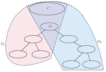
Figure 1: Subinstances created by a recursive call

We proceed by replacing $\bf x$ by $({\bf x}\setminus M)$. For the sake of clarity, we denote ${\bf x}^{*}=({\bf x}\setminus M)$. By Lemmata 13 and 14, to prove Lemma 11, it is now sufficient to return a solution that is at least ${\sf opt}$ and at most $\displaystyle{(1/(1+3\cdot(\frac{c\cdot\log n+9}{c\cdot\log n})^{\delta}\cdot\frac{1}{c\cdot\log n}))\cdot(\frac{c\cdot\log n}{c\cdot\log n+9})^{\delta-1}\cdot\log\alpha(G^{\prime})\cdot w({\bf x}^{*})}$, along with a set that realizes it. Moreover, for any $v\in V(G^{\prime})$, it holds that ${\bf x}^{*}(v)<\displaystyle{(1+3\cdot(\frac{c\cdot\log n+9}{c\cdot\log n})^{\delta}}$ $\displaystyle{\cdot\frac{1}{c\cdot\log n})\cdot(\frac{c\cdot\log n+9}{c\cdot\log n})^{\delta}}$ $\displaystyle{\cdot\frac{1}{c\cdot\log n}}$. Note that by Observation 16, by setting $c\geq 9q$, we have that $\displaystyle{(\frac{c\cdot\log n+9}{c\cdot\log n})^{\delta}\leq e<3}$, and therefore $\displaystyle{1+3\cdot(\frac{c\cdot\log n+9}{c\cdot\log n})^{\delta}\cdot\frac{1}{c\cdot\log n}\leq\frac{c\cdot\log n+9}{c\cdot\log n}}$. In particular, to prove Lemma 11, it is sufficient to return a solution that is at least ${\sf opt}$ and at most $\displaystyle{(\frac{c\cdot\log n}{c\cdot\log n+9})^{\delta}\cdot\log\alpha(G^{\prime})\cdot w({\bf x}^{*})}$.

Next, we define two subinstances, $I_{1}=(G_{1},w|_{V(G_{1})},C,H_{1},{\bf x}^{*}|_{V(G_{1})})$ and $I_{2}=(G_{2},w|_{V(G_{2})},$ $C,H_{2},{\bf x}^{*}|_{V(G_{2})})$ (see Figure 1). We solve each of these subinstances by a recursive call to CVD-APPROX (by the above discussion, these calls are valid — we satisfy the low-value and zero-clique invariants). Thus, we obtain two solutions, $s_{1}$ to $I_{1}$ and $s_{2}$ to $I_{2}$, and two sets that realize these solutions, $S_{1}$ and $S_{2}$. By the inductive hypothesis, we have the following observations.

Observation 17.

$S_{1}\cup S_{2}$ intersects any chordless cycle in $G^{\prime}$ that lies entirely in either $G_{1}$ or $G_{2}$.

Observation 18.

Given $i\in\{1,2\}$, $s_{i}\leq(\frac{c\cdot\log n}{c\cdot\log n+9})^{\delta}\cdot c\cdot\log(\alpha(G_{i}))\cdot w({\bf x}^{*}_{i})$.

Moreover, since ${\bf x}^{*}(V(C)\cup V(M))=0$, we also have the following observation.

Observation 19.

$w({\bf x}^{*}_{1})+w({\bf x}^{*}_{2})=w({\bf x}^{*})$.

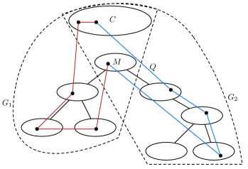
Figure 2: An illustration of a bad cycle

We say that a cycle of $G^{\prime}$ is bad if it is a chordless cycle that belongs entirely to neither $G_{1}$ nor $G_{2}$ (see Figure 2). Next, we show how to intersect bad cycles.

Bad Cycles. For any pair $(v,u)$ of vertices $v\in V(C)$ and $u\in V(M)$, we let ${\cal P}_{1}(v,u)$ denote the set of any (simple) path $P_{1}$ between $v$ and $u$ whose internal vertices belong only to $G_{1}$ and which does not contain a vertex $v^{\prime}\in C$ and a vertex $u^{\prime}\in M$ such that $\{v^{\prime},u^{\prime}\}\in E(G^{\prime})$. Symmetrically, we let ${\cal P}_{2}(v,u)$ denote the set of any path $P_{2}$ between $v$ and $u$ whose internal vertices belong only to $G_{2}$ and which does not contain a vertex $v^{\prime}\in C$ and a vertex $u^{\prime}\in M$ such that $\{v^{\prime},u^{\prime}\}\in E(G^{\prime})$. We note here that when $\{v,u\}\in E(G^{\prime})$ then ${\cal P}_{1}(v,u)={\cal P}_{2}(v,u)=\emptyset$.

We first examine the relation between bad cycles and pairs $(v,u)$ of vertices $v\in V(C)$ and $u\in V(M)$.

Lemma 20.

For any bad cycle $Q$ there exist a pair $(v,u)$ of vertices $v\in V(C)$, $u\in V(M)$, a path $P_{1}\in{\cal P}_{1}(v,u)$ such that $V(P_{1})\subseteq V(Q)$, and a path $P_{2}\in{\cal P}_{2}(v,u)$ such that $V(P_{2})\subseteq V(Q)$.

Proof.

Let $Q$ be some bad cycle. By the definition of a bad cycle, $Q$ must contain at least one vertex $a$ from $H_{1}\setminus V(M)$ and at least one vertex $b$ from $H_{2}\setminus V(M)$. Since $C$ and $M$ are cliques, $Q$ can contain at most two vertices from $C$ and at most two vertices from $M$, and if it contains two vertices from $C$ (resp. $M$), then these two vertices are neighbors. Moreover, since the set $V(C)\cup V(M)$ contains all vertices common to $G_{1}$ and $G_{2}$, $Q$ must contain at least one vertex $v\in V(C)$ and at least one vertex $u\in V(M)$ with $\{v,u\}\notin E(G^{\prime})$. Overall, we conclude that the subpath of $Q$ between $v$ and $u$ that contains $a$ belongs to ${\cal P}_{1}(v,u)$, while the subpath of $Q$ between $v$ and $u$ that contains $b$ belongs to ${\cal P}_{2}(v,u)$. ∎

In light Lemma 20, to intersect bad cycles, we now examine how the fractional solution ${\bf x}^{*}$ handles pairs $(v,u)$ of vertices $v\in V(C)$ and $u\in V(M)$.

Lemma 21.

For each pair $(v,u)$ of vertices $v\in V(C)$ and $u\in V(M)$ with $\{v,u\}\notin E(G^{\prime})$, there exists $i\in\{1,2\}$ such that for any path $P\in{\cal P}_{i}(v,u)$, ${\bf x}^{*}(V(P))\geq 1/2$.

Proof.

Suppose, by way of contradiction, that the lemma is incorrect. Thus, there exist a pair $(v,u)$ of vertices $v\in V(C)$ and $u\in V(M)$ with $\{v,u\}\notin E(G^{\prime})$, a path $P_{1}\in{\cal P}_{1}(v,u)$ such that ${\bf x}^{*}(V(P_{1}))<1/2$, and a path $P_{2}\in{\cal P}_{2}(v,u)$ such that ${\bf x}^{*}(V(P_{2}))<1/2$. Since ${\bf x}^{*}$ is a valid fractional solution, we deduce that $G^{\prime}[V(P_{1})\cup V(P_{2})]$ does not contain any chordless cycle. Consider a shortest subpath $\widehat{P}_{1}$ of $P_{1}$ between a vertex $a_{1}\in V(C)$ and a vertex $b_{1}\in V(M)$, and a shortest subpath $\widehat{P}_{2}$ of $P_{2}$ between a vertex $a_{2}\in V(C)$ and a vertex $b_{2}\in V(M)$. Since neither $P_{1}$ nor $P_{2}$ contains any edge such that one of its endpoints belongs to $V(C)$ while the other endpoint belongs to $V(M)$, we have that $|V(\widehat{P}_{1})|,|V(\widehat{P}_{2})|\geq 3$. Furthermore, since vertices common in $P_{1}$ and $P_{2}$ must belong to $V(C)\cup V(M)$, we have that $\widehat{P}_{1}$ does not contain internal vertices that belong to $\widehat{P}_{2}$ or adjacent to internal vertices on $\widehat{P}_{2}$. Overall, since $C$ and $M$ are cliques, we deduce that $G^{\prime}[V(\widehat{P}_{1})\cup V(\widehat{P}_{2})]$ contains a chordless cycle. To see this, let $a$ be the vertex closest to $b_{2}$ on $\widehat{P}_{2}$ that is a neighbor of $a_{1}$. Observe that $a$ exists as $a_{1}$ and $a_{2}$ are neighbors, and $a\neq b_{2}$. Moreover, we assume without loss of generality that if $a=a_{2}$, then $a_{2}$ has no neighbor on $\widehat{P}_{1}$ apart from $a_{1}$. Now, let $b$ be the vertex closest to $a$ on the subpath of $\widehat{P}_{2}$ between $a$ and $b_{2}$ that is a neighbor of $b_{1}$. If $b\neq b_{2}$, then the vertex-sets of $\widehat{P}_{1}$ and the subpath of $\widehat{P}_{1}$ between $a$ and $b$ together induce a chordless cycle. Else, let $b^{\prime}$ be the vertex closest to $a_{1}$ on $\widehat{P}_{1}$ that is a neighbor of $b_{2}$. Then, the vertex-sets of the subpath of $\widehat{P}_{1}$ between $a_{1}$ and $b^{\prime}$ and the subpath of $\widehat{P}_{1}$ between $a$ and $b_{2}$ together induce a chordless cycle. Since $G^{\prime}[V(\widehat{P}_{1})\cup V(\widehat{P}_{2})]$ is an induced subgraph of $G^{\prime}[V(P_{1})\cup V(P_{2})]$, we have reached a contradiction. ∎

Given $i\in\{1,2\}$, let $2{\bf x}^{*}_{i}$ denote the fractional solution that assigns to each vertex the value assigned by ${\bf x}^{*}_{i}$ times 2. Moreover, let $\widehat{G}_{1}=G_{1}\setminus(V(C)\cup V(M))$ and $\widehat{G}_{2}=G_{2}\setminus(V(C)\cup V(M))$. Observe that $\widehat{G}_{1}$ and $\widehat{G}_{2}$ are chordal graphs. Now, for every pair $(v,u)$ such that $v\in V(C),u\in V(M)$, we perform the following operation. We initialize ${\cal T}_{1}(v,u)=\emptyset$. Next, we consider every pair $(v^{\prime},u^{\prime})$ such that $v^{\prime}\in V(C)$, $u^{\prime}\in V(M)$, $\{v,v^{\prime}\}\cap N_{G_{1}}(u^{\prime})=\emptyset$ and $\{u,u^{\prime}\}\cap N_{G_{1}}(v^{\prime})=\emptyset$, and insert each pair in $\{(a,b):a\in N_{G_{1}}(v^{\prime})\cap V(\widehat{G}_{1}),b\in N_{G_{1}}(u^{\prime})\cap V(\widehat{G}_{1}),\widehat{G}_{1}$ has a path between $a$ and $b\}$ into ${\cal T}_{1}(v,u)$. We remark that the vertices in a pair in ${\cal T}_{1}(v,u)$ are not necessarily distinct. The definition of ${\cal T}_{2}(v,u)$ is symmetric to the one of ${\cal T}_{1}(v,u)$.

The following lemma translates Lemma 21 into an algorithm.

Lemma 22.

For each pair $(v,u)$ of vertices $v\in V(C)$, $u\in V(M)$ and $\{v,u\}\notin E(G^{\prime})$, one can compute (in polynomial time) an index $i(v,u)\in\{1,2\}$ such that for any path $P\in{\cal P}_{i}(v,u)$, $2{\bf x}^{*}_{i}(V(P))\geq 1$.

Proof.

Let $(v,u)$ be a pair of vertices such that $v\in V(C)$, $u\in V(M)$ and $\{v,u\}\notin E(G^{\prime})$. If there is $i\in\{1,2\}$ such that $P\in{\cal P}_{i}(v,u)=\emptyset$, then we have trivially obtained the required index which is $i(v,u)=i$. Otherwise, we proceed as follows. For any index $j\in\{1,2\}$, we perform the following procedure. For each pair $(a,b)\in{\cal T}_{i}(v,u)$, we use Dijkstra’s algorithm to compute the minimum weight of a path between $a$ and $b$ in the graph $\widehat{G}_{i}$ where the weights are given by $2{\bf x}^{*}_{i}$. In case for every pair $(a,b)$ the minimum weight is at least 1, we have found the desired index $i(v,u)$. Moreover, by Lemma 21 and since for all $v^{\prime}\in V(C)\cup V(M)$ it holds that ${\bf x}^{*}_{1}(v^{\prime})={\bf x}^{*}_{2}(v^{\prime})=0$, for at least one index $j\in\{1,2\}$, the maximum weight among the minimum weights associated with the pairs $(a,b)$ should be at least 1 (if this value is at least 1 for both indices, we arbitrarily decide to fix $i(v,u)=1$). ∎

At this point, we need to rely on approximate solutions to Weighted Multicut in chordal graphs (in this context, we will employ the algorithm given by Theorem 5 in Section 5). Here, a fractional solution ${\bf y}$ is a function ${\bf y}:V(G^{\prime})\rightarrow[0,\infty)$ such that for every pair $(s_{i},t_{i})\in{\cal T}$ and any path $P$ between $s_{i}$ and $t_{i}$, it holds that ${\bf y}(V(P))\geq 1$. An optimal fractional solution minimizes the weight $w({\bf y})=\sum_{v\in V(G^{\prime})}w(v)\cdot{\bf y}(v)$. Let fopt denote the weight of an optimal fractional solution.

By first employing the algorithm given by Lemma 22, we next construct two instances of Weighted Multicut. The first instance is $J_{1}=(\widehat{G}_{1},w_{1},{\cal T}_{1})$ and the second instance is $J_{2}=(\widehat{G}_{2},w_{2},{\cal T}_{2})$, where the sets ${\cal T}_{1}$ and ${\cal T}_{2}$ are defined as follows. We initialize ${\cal T}_{1}=\emptyset$. Now, for every pair $(v,u)$ such that $v\in V(C),u\in V(M)$, $i(v,u)=1$ and ${\cal P}_{1}(v,u)\neq\emptyset$, we insert each pair in ${\cal T}_{1}(v,u)$ into ${\cal T}_{1}$. The definition of ${\cal T}_{2}$ is symmetric to the one of ${\cal T}_{1}$.

By Lemma 22 and since for all $v\in V(C)\cup V(M)$ it holds that ${\bf x}^{*}_{1}(v)={\bf x}^{*}_{2}(v)=0$, we deduce that $2{\bf x}^{*}_{1}$ and $2{\bf x}^{*}_{2}$ are valid solutions to $J_{1}$ and $J_{2}$, respectively. Thus, by calling the algorithm given by Theorem 5 with each instance, we obtain a solution $r_{1}$ to the first instance, along with a set $R_{1}$ that realizes it, such that $r_{1}\leq 2d\cdot w({\bf x}^{*}_{1})$, and we also obtain a solution $r_{2}$ to the second instance, along with a set $R_{2}$ that realizes it, such that $r_{2}\leq 2d\cdot w({\bf x}^{*}_{2})$, for some fixed constant $d$.

By Observation 17 and Lemma 20, we obtained a set $S^{*}=S_{1}\cup S_{2}\cup R_{1}\cup R_{2}$ for which we have the following observation.

Observation 23.

$S^{*}$ intersects any chordless cycle in $G^{\prime}$, and it holds that $w(S^{*})\leq s_{1}+s_{2}+r_{1}+r_{2}$.

Recall that to prove Lemma 11 we need to show that $s_{1}+s_{2}+r_{1}+r_{2}\leq(\frac{c\cdot\log n}{c\cdot\log n+9})^{\delta-1}\cdot c\cdot\log(\alpha(G^{\prime}))\cdot w^{\prime}({\bf x})$ and we have $\delta\geq 2$. Furthermore, we have $(\frac{c\cdot\log n}{c\cdot\log n+9})^{\delta}\cdot c\cdot\log(\alpha(G^{\prime}))\cdot w^{\prime}({\bf x})\leq(\frac{c\cdot\log n}{c\cdot\log n+9})^{\delta-1}\cdot c\cdot\log(\alpha(G^{\prime}))\cdot w^{\prime}({\bf x})$. This together with Lemma 14 implies that it is enough to show $s_{1}+s_{2}+r_{1}+r_{2}\leq(\frac{c\cdot\log n}{c\cdot\log n+9})^{\delta}\cdot c\cdot\log(\alpha(G^{\prime}))\cdot w({\bf x}^{*})$. Recall that for any $i\in\{1,2\}$, $r_{i}\leq 2d\cdot w({\bf x}^{*}_{i})$. Thus, by Observation 18 and since for any $i\in\{1,2\}$, $\alpha(G_{i})\leq\frac{3}{4}\alpha(G^{\prime})$, we have that

$$w(S^{*})\leq(\frac{c\cdot\log n}{c\cdot\log n+9})^{\delta}\cdot c\cdot\log(\frac{3}{4}\alpha(G^{\prime}))\cdot(w({\bf x}^{*}_{1})+w({\bf x}^{*}_{2}))+2d\cdot(w({\bf x}^{*}_{1})+w({\bf x}^{*}_{2})).$$

By Observation 19, we further deduce that

$$w^{*}(S^{*})\leq\left((\frac{c\cdot\log n}{c\cdot\log n+9})^{\delta}\cdot c\cdot\log(\frac{3}{4}\alpha(G^{\prime}))+2d\right)\cdot w({\bf x}^{*}).$$

Now, it only remains to show that $(\frac{c\log n}{c\log n+9})^{\delta}\cdot c\cdot\log(\frac{3}{4}\alpha(G^{\prime}))+2d\leq(\frac{c\log n}{c\log n+9})^{\delta}\cdot c\cdot\log\alpha(G^{\prime})$, which is equivalent to $2d\leq(\frac{c\log n}{c\log n+9})^{\delta}\cdot c\cdot\log(\frac{4}{3})$. Recall that $\delta\leq q\cdot\log n$ (Observation 16). Thus, it is sufficient that we show that $2d\leq(\frac{c\log n}{c\log n+9})^{q\cdot\log n}\cdot c\cdot\log(\frac{4}{3})$. However, the term $(\frac{c\log n}{c\log n+9})^{q\cdot\log n}$ is lower bounded by $1/e^{9q}$. In other words, it is sufficient that we fix $c\geq 2\cdot e^{9q}\cdot d\cdot 1/\log(\frac{4}{3})$.

4.2 General Graphs

In this subsection we handle general instances by developing a $d\cdot\log^{2}n$-factor approximation algorithm for WCVD, Gen-CVD-APPROX, thus proving the correctness of Theorem 2. The exact value of the constant $d\geq\max\{96,2c\}$ is determined later. This algorithm is based on recursion, and during its execution, we often encounter instances that are of the form of the Clique+Chordal special case of WCVD, which will be dealt with using the algorithm CVD-APPROX of Section 4.1.

Recursion. We define each call to our algorithm Gen-CVD-APPROX to be of the form $(G^{\prime},w^{\prime})$, where $(G^{\prime},w^{\prime})$ is an instance of WCVD such that $G^{\prime}$ is an induced subgraph of $G$, and we denote $n^{\prime}=|V(G^{\prime})|$. We ensure that after the initialization phase, the graph $G^{\prime}$ never contains chordless cycles on at most 48 vertices. We call this invariant the $C_{48}$-free invariant. In particular, this guarantee ensures that the graph $G^{\prime}$ always contains only a small number of maximal cliques:

Lemma 24 ([11, 41]).

The number of maximal cliques of a graph $G^{\prime}$ that has no chordless cycles on four vertices is bounded by ${\mathcal{O}}({n^{\prime}}^{2})$, and they can be enumerated in polynomial time using a polynomial delay algorithm.

Goal. For each recursive call Gen-CVD-APPROX$(G^{\prime},w^{\prime})$, we aim to prove the following.

Lemma 25.

Gen-CVD-APPROX returns a solution that is at least ${\sf opt}$ and at most $\frac{d}{2}\cdot\log^{2}n^{\prime}\cdot{\sf opt}$. Moreover, it returns a subset $U\subseteq V(G^{\prime})$ that realizes the solution.

At each recursive call, the size of the graph $G^{\prime}$ becomes smaller. Thus, when we prove that Lemma 25 is true for the current call, we assume that the approximation factor is bounded by $\frac{d}{2}\cdot\log^{2}\widehat{n}\cdot{\sf opt}$ for any call where the size $\widehat{n}$ of the vertex-set of its graph is strictly smaller than $n^{\prime}$.

Initialization. Initially, we set $(G^{\prime},w^{\prime})=(G,w)$. However, we need to ensure that the $C_{48}$-free invariant is satisfied. For this purpose, we update $G^{\prime}$ as follows. First, we let ${\cal C}_{48}$ denote the set of all chordless cycles on at most 48 vertices of $G^{\prime}$. Clearly, ${\cal C}_{48}$ can be computed in polynomial time and it holds that $|{\cal C}_{48}|\leq n^{48}$. Now, we construct an instance of Weighted 48-Hitting Set, where the universe is $V(G^{\prime})$, the family of 48-sets is ${\cal C}_{48}$, and the weight function is $w^{\prime}$. Since each chordless cycle must be intersected, it is clear that the optimal solution to our Weighted 48-Hitting Set instance is at most ${\sf opt}$. By using the standard $c^{\prime}$-approximation algorithm for Weighted $c^{\prime}$-Hitting Set [27], which is suitable for any fixed constant $c^{\prime}$, we obtain a set $S\subseteq V(G^{\prime})$ that intersects all cycles in ${\cal C}_{48}$ and whose weight is at most $48\cdot{\sf opt}$. Having the set $S$, we remove its vertices from $G^{\prime}$. Now, the $C_{48}$-free invariant is satisfied, which implies that we can recursively call our algorithm. To the outputted solution, we add $w(S)$ and $S$. If Lemma 25 is true, we obtain a solution that is at most $\frac{d}{2}\cdot\log^{2}n\cdot{\sf opt}+48\cdot{\sf opt}\leq d\cdot\log^{2}n\cdot{\sf opt}$, which allows us to conclude the correctness of Theorem 2. We remark that during the execution of our algorithm, we only update $G^{\prime}$ by removing vertices from it, and thus it will always be safe to assume that the $C_{48}$-free invariant is satisfied.

Termination. Observe that due to Lemma 24, we can test in polynomial time whether $G^{\prime}$consists of a clique and a chordal graph: we examine each maximal clique of $G^{\prime}$, and check whether after its removal we obtain a chordal graph. Once $G^{\prime}$ becomes such a graph that consists of a chordal graph and a clique, we solve the instance $(G^{\prime},w^{\prime})$ by calling algorithm CVD-APPROX. Since $c\cdot\log n^{\prime}\leq\frac{d}{2}\cdot\log^{2}n^{\prime}$, we thus ensure that at the base case of our induction, Lemma 25 holds.

Recursive Call. For the analysis of a recursive call, let $S^{*}$ denote a hypothetical set that realizes the optimal solution ${\sf opt}$ of the current instance $(G^{\prime},w^{\prime})$. Moreover, let $(F,\beta)$ be a clique forest of $G^{\prime}-S^{*}$, whose existence is guaranteed by Lemma 1. Using standard arguments on forests, we have the following observation.

Observation 26.

There exist a maximal clique $M$ of $G^{\prime}$ and a subset $S\subseteq V(G^{\prime})\setminus M$ of weight at most ${\sf opt}$ such that $M\cup S$ is a balanced separator for $G^{\prime}$.

The following lemma translates this observation into an algorithm.

Lemma 27.

There is a polynomial-time algorithm that finds a maximal clique $M$ of $G^{\prime}$ and a subset $S\subseteq V(G^{\prime})\setminus M$ of weight at most $q\cdot\log n^{\prime}\cdot{\sf opt}$ for some fixed constant $q$ such that $M\cup S$ is a balanced separator for $G^{\prime}$.

Proof.

We examine every maximal clique of $G^{\prime}$. By Lemma 24, we need only consider ${\mathcal{O}}({n^{\prime}}^{2})$ maximal cliques, and these cliques can be enumerated in polynomial time. For each such clique $M$, we run the $q\cdot\log n^{\prime}$-factor approximation algorithm by Leighton and Rao [28] to find a balanced separator $S_{M}$ of $G^{\prime}-M$. Here, $q$ is some fixed constant. We let $S$ denote some set of minimum weight among the sets in $\{S_{M}:M$ is a maximal clique of $G^{\prime}\}$. By Observation 26, $w(S)\leq q\cdot\log n^{\prime}\cdot{\sf opt}$. Thus, the desired output is a pair $(M,S)$ where $M$ is one of the examined maximal cliques such that $S_{M}=S$. ∎

We call the algorithm in Lemma 27 to obtain a pair $(M,S)$. Since $M\cup S$ is a balanced separator for $G^{\prime}$, we can partition the set of connected components of $G^{\prime}-(M\cup S)$ into two sets, ${\cal A}_{1}$ and ${\cal A}_{2}$, such that for $V_{1}=\bigcup_{A\in{\cal A}_{1}}V(A)$ and $V_{2}=\bigcup_{A\in{\cal A}_{2}}V(A)$ it holds that $n_{1},n_{2}\leq\frac{2}{3}n^{\prime}$ where $n_{1}=|V_{1}|$ and $n_{2}=|V_{2}|$. We remark that we used the ${\mathcal{O}}(\log n)$-factor approximation algorithm by Leighton and Rao [28] in Lemma 27 to find the balanced separator instead of the ${\mathcal{O}}(\sqrt{\log n})$-factor approximation algorithm by Feige et al. [12], as the algorithm by Feige et al. is randomized.

Next, we define two inputs of (the general case of) WCVD: $I_{1}=(G^{\prime}[V_{1}],w^{\prime}|_{V_{1}})$ and $I_{2}=(G^{\prime}[V_{2}],w^{\prime}|_{V_{2}})$. Let ${\sf opt}_{1}$ and ${\sf opt}_{2}$ denote the optimal solutions to $I_{1}$ and $I_{2}$, respectively. Observe that since $V_{1}\cap V_{2}=\emptyset$, it holds that ${\sf opt}_{1}+{\sf opt}_{2}\leq{\sf opt}$. We solve each of the subinstances by recursively calling algorithm Gen-CVD-APPROX. By the inductive hypothesis, we thus obtain two sets, $S_{1}$ and $S_{2}$, such that $G^{\prime}[V_{1}]-S_{1}$ and $G^{\prime}[V_{2}]-S_{2}$ are chordal graphs, and $w^{\prime}(S_{1})\leq\frac{d}{2}\cdot\log^{2}n_{1}\cdot{\sf opt}_{1}$ and $w^{\prime}(S_{2})\leq\frac{d}{2}\cdot\log^{2}n_{2}\cdot{\sf opt}_{2}$.

We proceed by defining an input of the Clique+Chordal special case of WCVD: $J=(G^{\prime}[(V_{1}\cup V_{2}\cup M)\setminus(S_{1}\cup S_{2})],w^{\prime}|_{(V_{1}\cup V_{2}\cup M)\setminus(S_{1}\cup S_{2})})$. Observe that since $G^{\prime}[V_{1}]-S_{1}$ and $G^{\prime}[V_{2}]-S_{2}$ are chordal graphs and $M$ is a clique, this is indeed an instance of the Clique+Chordal special case of WCVD. We solve this instance by calling algorithm CVD-APPROX. We thus obtain a set, $\widehat{S}$, such that $G^{\prime}[(V_{1}\cup V_{2}\cup M)-(S_{1}\cup S_{2}\cup\widehat{S})]$ is a chordal graphs, and $w^{\prime}(\widehat{S})\leq c\cdot\log n^{\prime}\cdot{\sf opt}$ (since $|(V_{1}\cup V_{2}\cup M)\setminus(S_{1}\cup S_{2})|\leq n^{\prime}$ and the optimal solution of each of the subinstances is at most ${\sf opt}$).

Observe that since $M$ is a clique and there is no edge in $E(G^{\prime})$ between a vertex in $V_{1}$ and a vertex in $V_{2}$, any chordless cycle of $G^{\prime}-(S\cup S_{1}\cup S_{2})$ entirely belongs to either $G^{\prime}[(V_{1}\cup M)\setminus S_{1}]$ or $G^{\prime}[(V_{2}\cup M)\setminus S_{2}]$. This observation, along with the fact that $G^{\prime}[(V_{1}\cup V_{2}\cup M)\setminus(S_{1}\cup S_{2}\cup\widehat{S})]$ is a chordal graphs, implies that $G^{\prime}-T$ is a chordal graphs where $T=S\cup S_{1}\cup S_{2}\cup\widehat{S}$. Thus, it is now sufficient to show that $w^{\prime}(T)\leq\frac{d}{2}\cdot\log^{2}n^{\prime}\cdot{\sf opt}$.

By the discussion above, we have that

$$\begin{array}[]{ll}w^{\prime}(T)&\leq w^{\prime}(S)+w^{\prime}(S_{1})+w^{\prime}(S_{2})+w^{\prime}(\widehat{S})\\ &\leq q\cdot\log n^{\prime}\cdot{\sf opt}+\frac{d}{2}\cdot(\log^{2}n_{1}\cdot{\sf opt}_{1}+\log^{2}n_{2}\cdot{\sf opt}_{2})+c\cdot\log n^{\prime}\cdot{\sf opt}.\end{array}$$

Recall that $n_{1},n_{2}\leq\frac{2}{3}n^{\prime}$ and ${\sf opt}_{1}+{\sf opt}_{2}\leq{\sf opt}$. Thus, we have that

$$\begin{array}[]{ll}w^{\prime}(T)&\leq q\cdot\log n^{\prime}\cdot{\sf opt}+\frac{d}{2}\cdot(\log^{2}\frac{2}{3}n^{\prime})\cdot{\sf opt}+c\cdot\log n^{\prime}\cdot{\sf opt}\\ &\leq\frac{d}{2}\cdot\log^{2}n^{\prime}\cdot{\sf opt}+(q+c-\frac{d}{2}\log\frac{3}{2})\cdot\log n^{\prime}\cdot{\sf opt}.\end{array}$$

Overall, we conclude that to ensure that $w^{\prime}(T)\leq\frac{d}{2}\cdot\log^{2}n^{\prime}\cdot{\sf opt}$, it is sufficient to ensure that $q+c-\frac{d}{2}\log\frac{3}{2}\leq 0$, which can be done by fixing $\displaystyle{d=\frac{2}{\log\frac{3}{2}}\cdot(q+c)}$.

5 Weighted Multicut in Chordal Graphs

In this section we prove Theorem 3. Let us denote $c=8$. Recall that for Weighted Multicut, a fractional solution ${\bf x}$ is a function ${\bf x}:V(G)\rightarrow[0,\infty)$ such that for every pair $(s,t)\in{\cal T}$ and any path $P$ between $s$ and $t$, it holds that ${\bf x}(V(P))\geq 1$. An optimal fractional solution minimizes the weight $w({\bf x})=\sum_{v\in V(G)}w(v)\cdot{\bf x}(v)$. Let fopt denote the weight of an optimal fractional solution. Theorem 3 follows from the next result, whose proof is the focus of this section.

Lemma 28.

Given an instance of Weighted Multicut in chordal graphs, one can find (in polynomial time) a solution that is at least ${\sf opt}$ and at most $4c\cdot{\sf fopt}$, along with a set that realizes it.

Preprocessing. By using the ellipsoid method, we may next assume that we have optimal fractional solution ${\bf x}$ at hand. We say that ${\bf x}$ is nice if for all $v\in V(G)$, there exists $i\in\{0\}\cup\mathbb{N}$ such that ${\bf x}(v)=\frac{i}{n}$. Let $h({\bf x})=\{v\in V(G):{\bf x}(v)\geq 1/c\}$ denote the set of vertices to which ${\bf x}$ assigns high values.

Lemma 29.

Define a function $\widehat{\bf x}:V(G)\rightarrow[0,\infty)$ as follows. For all $v\in V(G)$, if ${\bf x}(v)<1/2n$ then $\widehat{\bf x}(v)=0$, and otherwise $\widehat{\bf x}(v)$ is the smallest value of the form $i/n$, for some $i\in\mathbb{N}$, that is at least $2{\bf x}(v)$. Then, $\widehat{\bf x}$ is a fractional solution such that $w(\widehat{\bf x})\leq 4w({\bf x})$.

Proof.

To show that $\widehat{\bf x}$ is a fractional solution, consider some path $P$ between $s$ and $t$ such that $(s,t)\in{\cal T}$. Let $\ell^{\prime}({\bf x})=\{v\in V(G):{\bf x}(v)<1/2n\}$. We have that $\widehat{\bf x}(V(P))=\sum_{v\in V(P)\setminus\ell^{\prime}({\bf x})}\widehat{\bf x}(v)\geq 2\sum_{v\in V(P)\setminus\ell^{\prime}({\bf x})}{\bf x}(v)$. Thus, to show that $\widehat{\bf x}(V(P))\geq 1$, it is sufficient to show that $\frac{1}{2}\leq\sum_{v\in V(P)\setminus\ell^{\prime}({\bf x})}{\bf x}(v)$. Since ${\bf x}$ is a fractional solution, it holds that ${\bf x}(V(P))=\sum_{v\in V(P)\cap\ell^{\prime}({\bf x})}{\bf x}(v)+\sum_{v\in V(P)\setminus\ell^{\prime}({\bf x})}{\bf x}(v)\geq 1$. Thus, $1\leq\frac{1}{2n}|V(P)\cap\ell^{\prime}({\bf x})|+\sum_{v\in V(P)\setminus\ell^{\prime}({\bf x})}{\bf x}(v)$. Since $|V(P)\cap\ell^{\prime}({\bf x})|\leq n$, we conclude that $\frac{1}{2}\leq\sum_{v\in V(P)\setminus\ell^{\prime}({\bf x})}{\bf x}(v)$.

The second part of the claim follows from the observation that for all $v\in V(G)$, $\widehat{\bf x}(v)\leq 4{\bf x}(v)$. ∎

Accordingly, we update ${\bf x}$ to $\widehat{\bf x}$. Our preprocessing step also relies on the following standard lemma.

Lemma 30.

Define $\widehat{G}=G-h({\bf x})$, $\widehat{w}=w|_{V(\widehat{G})}$ and $\widehat{\bf x}={\bf x}|_{V(\widehat{G})}$. Then, $c\cdot w(\widehat{\bf x})+w(h({\bf x}))\leq c\cdot w({\bf x})$.

Proof.

By the definition of $h({\bf x})$, it holds that $w(\widehat{\bf x})\leq w({\bf x})-\frac{1}{c}w(h({\bf x}))$. Thus, $c\cdot w(\widehat{\bf x})+w(h({\bf x}))\leq c\cdot(w({\bf x})-\frac{1}{c}\cdot w(h({\bf x})))+w(h({\bf x}))=c\cdot w({\bf x})$. ∎

We thus further update $G$ to $\widehat{G}$, $w$ to $\widehat{w}$ and ${\bf x}$ to $\widehat{\bf x}$, where we ensure that once we obtain a solution to the new instance, we add $w(h({\bf x}))$ to this solution and $h({\bf x})$ to the set realizing it. Overall, we may next focus only on the proof of the following lemma.

Lemma 31.

Let $(G,w)$ be an instance of Weighted Multicut in chordal graphs, and ${\bf x}$ be a nice fractional solution such that $h({\bf x})=\emptyset$. Then, one can find (in polynomial time) a solution that is at least ${\sf opt}$ and at most $c\cdot w({\bf x})$, along with a set that realizes it.

The Algorithm. Since $G$ is a chordal graph, we can first construct in polynomial time a clique forest $(F,\beta)$ of $G$ (Lemma 1). Without loss of generality, we may assume that $F$ is a tree, else $G$ is not a connected graph and we can handle each of its connected components separately. Now, we arbitrarily root $F$ at some node $r_{F}$, and we arbitrarily choose a vertex $r_{G}\in\beta(r_{F})$. We then use Dijkstra’s algorithm to compute (in polynomial time) for each vertex $v\in V(G)$, the value $\displaystyle{d(v)=\min_{P\in{\cal P}(v)}{\bf x}(V(P))}$, where ${\cal P}(v)$ is the set of paths in $G$ between $r_{G}$ and $v$.

We define $n+1$ bins: for all $i\in\{0,1,\ldots,n\}$, the bin $B_{i}$ contains every vertex $v\in V(G)$ for which there exists $j\in\{0\}\cup\mathbb{N}$ such that $d(v)-{\bf x}(v)<(\frac{i}{n}+2j)\frac{1}{c}\leq d(v)$ (i.e., $0\leq d(v)-(\frac{i}{n}+2j)\frac{1}{c}<{\bf x}(v)$). Let $B_{i^{*}}$, $i^{*}\in\{0,1,\ldots,n\}$, be a bin that minimizes $w(B_{i^{*}})$. The output consists of $w(B_{i^{*}})$ and $B_{i^{*}}$.

Approximation Factor. Given $r\in[0,1]$, let $\widehat{B}_{r}$ be the set that contains every vertex $v\in V(G)$ for which there exists $j\in\{0\}\cup\mathbb{N}$ such that $0\leq d(v)-(r+2j)\frac{1}{c}<{\bf x}(v)$. We start with the following claim.

Lemma 32.

There exists $r^{*}\in[0,1]$ such that $w(\widehat{B}_{r^{*}})\leq c\cdot w({\bf x})$.

Proof.

For any $d\geq 0$, observe that there exists exactly one $j\in\{0\}\cup\mathbb{N}$ for which there exists $r\in[0,1]$ such that $0\leq d-(r+2j)\frac{1}{c}<\frac{1}{c}$, and denote it by $j(d)$. Suppose that we choose $r\in[0,1]$ uniformly at random. Consider some vertex $v\in V(G)$. Then, since $h({\bf x})=\emptyset$, the probability that there exists $j\in\{0\}\cup\mathbb{N}$ such that $0\leq d(v)-(r+2j)\frac{1}{c}<{\bf x}(v)$ is equal to the probability that $0\leq d(v)-(r+2j(d(v)))\frac{1}{c}<{\bf x}(v)$. Now, the probability that $0\leq d(v)-(r+2j(d(v)))\frac{1}{c}<{\bf x}(v)$ is equal to $c\cdot{\bf x}(v)$. The expected weight $w(\widehat{B}_{r})$ is $c\cdot\sum_{v\in V(G)}{\bf x}(v)\cdot w(v)=c\cdot w({\bf x})$. Thus, there exists $r^{*}\in[0,1]$ such that $w(\widehat{B}_{r^{*}})\leq c\cdot w({\bf x})$. ∎

Now, the proof of the approximation factor follows from the next claim.

Lemma 33.

There exists $i\in\{0,1,\ldots,n\}$ such that $B_{i}\subseteq\widehat{B}_{r^{*}}$.

Proof.

Let $i$ be the smallest index in $\{0,1,\ldots,n\}$ such that $r^{*}\leq\frac{i}{n}$. Consider some vertex $v\in B_{i}$. Then, for some $j\in\{0\}\cup\mathbb{N}$, $d(v)-{\bf x}(v)<(\frac{i}{n}+2j)\frac{1}{c}\leq d(v)$. Since $r^{*}\leq\frac{i}{n}$, we have that $(r^{*}+2j)\frac{1}{c}\leq d(v)$. Since $\bf x$ is nice, it holds that there exists $t\in\{0\}\cup\mathbb{N}$ such that $d(v)-{\bf x}(v)=\frac{t}{n}$. Thus, for any $p<\frac{1}{n}$, it holds that $d(v)-{\bf x}(v)<(\frac{i}{n}+2j-p)\frac{1}{c}$. By the choice of $i$, $\frac{i}{n}-r^{*}<\frac{1}{n}$, and therefore $d(v)-{\bf x}(v)<(r^{*}+2j)\frac{1}{c}$, which implies that $v\in\widehat{B}_{r^{*}}$. ∎

Feasibility. We need to prove that for any pair $(s,t)\in{\cal T}$, $G-B_{i^{*}}$ does not have any path between $s$ and $t$. Consider some path $P=(v_{1},v_{2},\cdots,v_{\ell})$ between $s$ and $t$. Here, $v_{1}=s$ and $v_{\ell}=t$. Suppose, by way of contradiction, that $V(P)\cap B_{i^{*}}=\emptyset$. Then, for all $v_{i}\in V(P)$, it holds that there is no $j\in\{0\}\cup\mathbb{N}$ such that $0\leq d(v_{i})-(\frac{i^{*}}{n}+2j)\frac{1}{c}<{\bf x}(v_{i})$.

Let $s\in V(F)$ be the closest node to $r_{F}$ that satisfies $\beta(s)\cap V(P)\neq\emptyset$ (since $F$ is a clique tree and $P$ is a path, the node $s$ is uniquely defined). Let $v_{\widehat{i}}$ be some vertex in $\beta(s)\cap V(P)\neq\emptyset$. For the sake of clarity, let us denote the subpath of $P$ between $v_{\widehat{i}}$ and $v_{\ell}$ by $Q=(u_{1},u_{2},\cdots,u_{t})$, where $u_{1}=v_{\widehat{i}}$ and $u_{t}=v_{\ell}$. Let $j^{*}$ be the smallest value in $\{0\}\cup\mathbb{N}$ that satisfies $d(u_{1})-{\bf x}(u_{1})<(\frac{i^{*}}{n}+2j^{*})\frac{1}{c}$. Note that $d(u_{1})<(\frac{i^{*}}{n}+2j^{*})\frac{1}{c}$. It is thus well defined to let $p$ denote the largest index in $[t]$ such that $d(u_{p})<(\frac{i^{*}}{n}+2j^{*})\frac{1}{c}$.

First, suppose that $p\in[t-1]$. We then have that $(\frac{i^{*}}{n}+2j^{*})\frac{1}{c}\leq d(u_{p+1})$. For all $2\leq i\leq t$, it holds that $d(u_{i})\leq d(u_{i-1})+{\bf x}(u_{i})$. We thus obtain that $d(u_{p+1})-{\bf x}(u_{p+1})\leq d(u_{p})<(\frac{i^{*}}{n}+2j^{*})\frac{1}{c}$. This statement implies that $u_{p+1}\in B_{i^{*}}$, which is a contradiction.

Now, we suppose that $p=t$. Note that $(\frac{i^{*}}{n}+2j^{*}-2)\frac{1}{c}\leq d(u_{1})-{\bf x}(u_{1})$ (by the minimality of $j^{*}$), and $d(u_{t})<(\frac{i^{*}}{n}+2j^{*})\frac{1}{c}$. We get that $d(u_{t})<d(u_{1})-{\bf x}(u_{1})+\frac{2}{c}$. In other words, $d(u_{t})-d(u_{1})+{\bf x}(u_{1})<\frac{2}{c}$. Let des$(s)$ denote the set consisting of $s$ and its descendants in $F$. Since $F$ is a clique tree, we have that $V(Q)\subseteq\bigcup_{s^{\prime}\in\mathrm{des}(s)}\beta(s^{\prime})$. Thus, any path from $r_{G}$ to $u_{t}$ that realizes $d(u_{t})$ contains a vertex from $\beta(s)$. Since there exists a path from $r_{G}$ to $u_{t}$ that realizes $d(u_{t})$, we deduce that there exists a path, $P_{t}$, from $r_{G}$ to $u_{t}$ that realizes $d(u_{t})$ and contains a vertex $x\in N_{G}[u_{1}]$. Let $P^{*}_{t}$ denote the subpath of $P_{t}$ between $x$ and $u_{t}$, and let $P^{*}$ denote the path that starts at $u_{1}$ and then traverses $P^{*}_{t}$. Then, ${\bf x}(V(P^{*}))\leq{\bf x}(u_{1})+{\bf x}(V(P^{*}_{t}))={\bf x}(u_{1})+d(u_{t})-d(x)+{\bf x}(x)$. Note that $d(u_{1})\leq d(x)+{\bf x}(u_{1})$, and therefore ${\bf x}(V(P^{*}))\leq{\bf x}(u_{1})+d(u_{t})-(d(u_{1})-{\bf x}(u_{1}))+{\bf x}(x)={\bf x}(u_{1})+{\bf x}(x)+(d(u_{t})-d(u_{1})+{\bf x}(u_{1}))$. Since $h({\bf x})=\emptyset$ and $d(u_{t})-d(u_{1})+{\bf x}(u_{1})<\frac{2}{c}$, we get that ${\bf x}(V(P^{*}))<\frac{4}{c}$. The symmetric analysis of the subpath of $P$ between $u_{1}=v_{\widehat{i}}$ and $v_{1}$ shows that there exists a path $P^{**}$ between $u_{1}$ and $v_{1}$ such that ${\bf x}(V(P^{**}))<\frac{4}{c}$. Overall, we get that there exists a path, $P^{\prime}$, between $v_{1}=s$ and $v_{\ell}=u_{\ell}=t$ such that ${\bf x}(V(P^{\prime}))<\frac{8}{c}$. Since $c\geq 8$, we reach a contradiction to the assumption that ${\bf x}$ is a fractional solution.

6 Distance-Hereditary Vertex Deletion

In this section we prove Theorem 4. We start with preliminaries.

Preliminaries.

A graph $G$ is distance hereditary if every connected induced subgraph $H$ of $G$, for all $u,v\in V(H)$ the number of vertices in shortest path between $u$ and $v$ in $G$ is same as the number of vertices in shortest path between $u$ and $v$ in $H$. Another characterization of distance hereditary graphs is the graph not containing an induced sub-graph isomorphic to a house, a gem, a domino or an induced cycle on $5$ or more vertices (refer Figure 3). We refer to a house, a gem, a domino or an induced cycle on at least $5$ vertices as a DH-obstruction. A DH-obstruction on at most $48$ vertices is a small DH-obstruction. A biclique is a graph $G$ with vertex bipartition $X,Y$ each of them being non-empty such that for each $x\in X$ and $y\in Y$ we have $\{x,y\}\in E(G)$. We note here that, $X$ and $Y$ need not be independent sets in a biclique $G$.

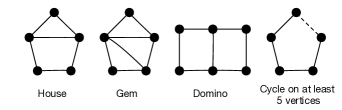
Figure 3: Obstruction set for distance hereditary graphs

Clearly, we can assume that the weight $w(v)$ of each vertex $v\in V(G)$ is positive, else we can insert $v$ into any solution. Our approximation algorithm for WDHVD comprises of two components. The first component handles the special case where the input graph $G$ consists of a biclique $C$ and a distance hereditary $H$. Here, we also assume that the input graph has no “small” DH-obstruction. We show that when input restricted to these special instances WDHVD admits an $\mathcal{O}(\log^{2}n)$-factor approximation algorithm.

The second component is a recursive algorithm that solves general instances of the problem. Initially, it easily handles “small” DH-obstruction. Then, it gradually disintegrates a general instance until it becomes an instance of the special form that can be solved in polynomial time. More precisely, given a problem instance, the algorithm divides it by finding a maximal biclique $M$ (using an exhaustive search which relies on the guarantee that $G$ has no “small” DH-obstruction) and a small separator $S$ (using an approximation algorithm) that together break the input graph into two graphs significantly smaller than their origin.

6.1 Biclique+ Distance Hereditary Graph

In this subsection we handle the special case where the input graph $G$ consists of a biclique $C$ and a distance hereditary graph $H$. More precisely, along with the input graph $G$ and the weight function $w$, we are also given a biclique $C$ and a distance hereditary graph $H$ such that $V(G)=V(C)\cup V(H)$, where the vertex-sets $V(C)$ and $V(H)$ are disjoint. Here, we also assume that $G$ has no DH-obstruction on at most $48$ vertices, which means that every DH-obstructionin $G$ is a chordless cycle of strictly more than $48$ vertices. Note that the edge-set $E(G)$ may contain edges between vertices in $C$ and vertices in $H$. We call this special case the Biclique + Distance Hereditary special case. Our objective is to prove the following result.

Lemma 34.

The Biclique + Distance Hereditary special case of WDHVD admits an ${\mathcal{O}}(\log^{2}n)$-factor approximation algorithm.

We assume that $n\geq 2^{12}$, else the input instance can be solve by brute-force . Let $c$ be a fixed constant (to be determined later). In the rest of this subsection, we design a $c\cdot\log n$-factor approximation algorithm for the Biclique + Distance Hereditary special case of WDHVD.

Recursion. Our approximation algorithm is a recursive algorithm. We call our algorithm DHD-APPROX, and define each call to be of the form $(G^{\prime},w^{\prime},C,H^{\prime},{\bf x})$. Here, $G^{\prime}$ is an induced subgraph of $G$ such that $V(C)\subseteq V(G^{\prime})$, and $H^{\prime}$ is an induced subgraph of $H$. The argument ${\bf x}$ is discussed below. We remark that we continue to use $n$ to refer to the size of the vertex-set of the input graph $G$ rather than the current graph $G^{\prime}$.

Arguments. While the execution of our algorithm progresses, we keep track of two arguments: the number of vertices in the current distance hereditary graph $H^{\prime}$ that are assigned a non-zero value by ${\bf x}$, which we denote by $\alpha(G^{\prime})$ and the fractional solution ${\bf x}$.

Observation 35.

The measure $\alpha(G^{\prime})$ can be computed in polynomial time.

A fractional solution ${\bf x}$ is a function ${\bf x}:V(G^{\prime})\rightarrow[0,\infty)$ such that for every chordless cycle $Q$ of $G^{\prime}$ on at least $5$ vertices it holds that ${\bf x}(V(Q))\geq 1$. An optimal fractional solution minimizes the weight $w^{\prime}({\bf x})=\sum_{v\in V(G^{\prime})}w^{\prime}(v)\cdot{\bf x}(v)$. Clearly, the solution to the instance $(G^{\prime},w^{\prime})$ of WDHVD is at least as large as the weight of an optimal fractional solution. Although we initially compute an optimal fractional solution ${\bf x}$ (at the initialization phase that is described below), during the execution of our algorithm, we manipulate this solution so it may no longer be optimal. Prior to any call to DHD-APPROX with the exception of the first call, we ensure that ${\bf x}$ satisfies the following invariants:

• Low-Value Invariant: For any $v\in V(G^{\prime})$, it holds that ${\bf x}(v)<1/\log n$.

• Zero-Biclique Invariant: For any $v\in V(C)$, it holds that ${\bf x}(v)=0$.

We note that the Low-Value Invariant used here is simpler than the one used in Section 4.1 since it is enough for the purpose of this section.

Goal. The depth of the recursion tree will be bounded by $\Delta={\mathcal{O}}(\log n)$, where the depth of initial call is $1$. The correctness of this claim is proved when we explain how to perform a recursive call. For each recursive call to DHD-APPROX$(G^{\prime},w^{\prime},C,H^{\prime},{\bf x})$, we aim to prove the following.

Lemma 36.

For any $\delta\in\{1,2,\ldots,\Delta\}$, each recursive call to DHD-APPROX of depth $\delta\geq 2$ returns a solution that is at least ${\sf opt}$ and at most $(\frac{\log n}{\log n+4})^{\delta}\cdot c\cdot\log n\cdot\log(\alpha(G^{\prime}))\cdot w^{\prime}({\bf x})$. Moreover, it returns a subset $U\subseteq V(G^{\prime})$ that realizes the solution.

At the initialization phase, we see that in order to prove Lemma 34, it is sufficient to prove Lemma 36.

Initialization. Initially, the graphs $G^{\prime}$ and $H^{\prime}$ are simply set to be the input graphs $G$ and $H$, and the weight function $w^{\prime}$ is simply set to be input weight function $w$. Moreover, we compute an optimal fractional solution ${\bf x}={\bf x}_{\mathrm{init}}$ by using the ellipsoid method. Recall that the following claim holds.

Observation 37.

The solution of the instance $(G^{\prime},w^{\prime})$ of WDHVD is lower bounded by $w^{\prime}({\bf x}_{\mathrm{init}})$.

Moreover, it holds that $\alpha(G^{\prime})\leq n$, and therefore to prove Lemma 34, it is sufficient to return a solution that is at least ${\sf opt}$ and at most $c\cdot\log n\cdot\log(\alpha(G))\cdot w({\bf x})$ (along with a subset that realizes the solution). Part of the necessity of the stronger claim given by Lemma 36 will become clear at the end of the initialization phase.

We would like to proceed by calling our algorithm recursively. For this purpose, we first need to ensure that ${\bf x}$ satisfies the low-value and zero-biclique invariants, to which end we use the following notation. We let $h({\bf x})=\{v\in V(G^{\prime}):{\bf x}(v)\geq 1/\log n\}$ denote the set of vertices to which ${\bf x}$ assigns high values. Note that we can assume for each $v\in h({\bf x})$, we have ${\bf x}(v)\leq 1$. Moreover, given a biclique $M$ in $G^{\prime}$, we let $({\bf x}\setminus M):V(G^{\prime})\rightarrow[0,\infty)$ denote the function that assigns 0 to any vertex in $M$ and $(1+\frac{4}{\log n}){\bf x}(v)$ to any other vertex $v\in V(G^{\prime})$. Now, to adjust ${\bf x}$ to be of the desired form both at this phase and at later recursive calls, we rely on the following lemmata.

Lemma 38.

Define $\widehat{G}=G^{\prime}-h({\bf x})$, $\widehat{w}=w^{\prime}|_{V(\widehat{G})}$ and $\widehat{\bf x}={\bf x}|_{V(\widehat{G})}$. Then, $c^{\prime}\cdot\log n\cdot\log(\alpha(\widehat{G}))\cdot w^{\prime}(\widehat{\bf x})+w^{\prime}(h({\bf x}))\leq c^{\prime}\cdot\log n\cdot\log(\alpha(G))\cdot w^{\prime}({\bf x})$, where $c^{\prime}\geq 1$.

Proof.

By the definition of $h({\bf x})$, it holds that $w^{\prime}(\widehat{\bf x})\leq w^{\prime}({\bf x})-\frac{1}{\log n}\cdot w^{\prime}(h({\bf x}))$. Since $\widehat{G}$ is an induced subgraph of $G^{\prime}$, it also holds that $\alpha(\widehat{G})\leq\alpha(G^{\prime})$. Thus, $c^{\prime}\cdot\log n\cdot\log(\alpha(\widehat{G}))\cdot w^{\prime}(\widehat{\bf x})+w^{\prime}(h({\bf x}))\leq c^{\prime}\cdot\log n\cdot\log(\alpha(G^{\prime}))\cdot(w^{\prime}({\bf x})-\frac{1}{\log n}\cdot w^{\prime}(h({\bf x})))+w^{\prime}(h({\bf x}))\leq c^{\prime}\cdot\log n\cdot\log(\alpha(G))\cdot w^{\prime}({\bf x})$. ∎

Thus, it is safe to update $G^{\prime}$ to $G^{\prime}-h({\bf x})$, $w^{\prime}$ to $w^{\prime}|_{V(\widehat{G})}$, $H^{\prime}$ to $H^{\prime}-h({\bf x})$ and ${\bf x}$ to ${\bf x}|_{V(\widehat{G})}$, where we ensure that once we obtain a solution to the new instance, we add $w^{\prime}(h({\bf x}))$ to this solution and $h({\bf x})$ to the set realizing it.

Lemma 39.

Let $Q$ be a chordless cycle on at least $5$ vertices and $M$ be a biclique in $G^{\prime}$ with vertex partitions as $V(M)=M_{1}\uplus M_{2}$ such that $V(Q)\cap V(M)\neq\emptyset$. Then there is a chordless cycle $Q^{\prime}$ on at least $5$ vertices that intersects $M$ in at most $3$ vertices such that $E(Q^{\prime}\setminus M)\subseteq E(Q\setminus M)$. Furthermore, $Q^{\prime}$ is of one of the following three types.

• $Q^{\prime}\cap M$ is a single vertex

• $Q^{\prime}\cap M$ is an edge in $G[M]$

• $Q^{\prime}\cap M$ is an induced path on $3$ vertices in $M$.

Proof.

Observe that no chordless cycle on $5$ or more vertices may contain two vertices from each of $M_{1}$ and $M_{2}$, as that would imply a chord in it. Now, if the chordless cycle $Q$ already satisfies the required conditions we output it as $Q^{\prime}$.

First consider the case, when $Q\cap M$ contains exactly two vertices that don’t have an edge between them. Then the two vertices, say $v_{1},v_{2}$, are both either in $M_{1}$ or in $M_{2}$. Suppose that they are both in $M_{1}$ and consider some vertex $u\in M_{2}$. Let $P_{1}$ is the longer of the two path segments of $Q$ between $v_{1}$ and $v_{2}$, and note that it must length at least $3$. Then observe that $G^{\prime}[P_{1}\cup\{u,v_{1},v_{2}\}]$ contains a DH-obstruction, as $v_{1},v_{2}$ have different distances depending on if $u$ is included in an induced subgraph or not. And further, it is easy to see that this DH-obstruction contains the induced path $v_{1},u,v_{2}$. However, as all small obstructions have been removed from the graph, we have that $Q^{\prime}$ is a chordless cycle in $G^{\prime}$ on at least $5$ vertices. Furthermore, $Q^{\prime}\cap M$ is the induced path $(v_{1},u,v_{2})$, in $G^{\prime}$ and $E(Q^{\prime}\setminus M)\subseteq E(Q\setminus M)$.

Now consider the case when $Q\cap M$ contains exactly three vertices. Observe that it cannot contain two vertices of $M_{1}$ and one vertex of $M_{2}$, or vice versa, as $Q$ doesn’t satisfy the required conditions. Therefore, $Q\cap M$ contains exactly three vertices from $M_{1}$ (or from $M_{2}$), which again don’t form an induced path of length $3$. So there is an independent set of size $2$ in $Q\cap M$, and now, as before, we can again obtain the chordless cycle $Q^{\prime}$ on at least $5$ vertices with $E(Q^{\prime}\setminus M)\subseteq E(Q\setminus M)$. Before we consider the other cases, we have the following claim.

Claim 1.

Let $M$ be a biclique in $G^{\prime}$ with vertex partition as $V(M)=M_{1}\uplus M_{2}$. Then $G^{\prime}[M]$ has no induced $P_{4}$.

Proof.

Let $P$ be any induced path of length $4$ in $G^{\prime}[M]$. Then, either $V(P)\subseteq M_{1}$ or $V(P)\subseteq M_{2}$. Now consider any such path $P$ in $M_{1}$ and some vertex $u\in M_{2}$. Then $G^{\prime}[P\cup\{u\}]$ contains a DH-obstruction of size $5$ which is a contradiction to the fact that $G^{\prime}$ has no small obstructions. ∎

Next, let $Q\cap M$ contain $4$ or more vertices. Note that in this case all these vertices are all either in $M_{1}$ or in $M_{2}$ since otherwise, $Q$ would not be a chordless cycle in $G^{\prime}$ on at least $5$ vertices. Let us assume these vertices lie in $M_{1}$ (other case is symmetric). Let $v_{1},v_{2},v_{3},\cdots,v_{\ell}\in M_{1}\cap Q$ be the sequence of vertices obtained when we traverse $Q$ starting from an arbitrary vertex, where $\ell\geq 4$. By Claim 1 they cannot form an induced path on $4$ vertices, i.e. $G^{\prime}[V(Q)\cap M_{1}]$ consists of at least two connected components. Without loss of generality we may assume that $v_{1}$ and $v_{\ell}$ are in different components. Observe that the only possible edges between these vertices may be at most two of the edges $(v_{1},v_{2}),(v_{2},v_{3})$, and $(v_{3},v_{\ell})$. Hence, we conclude that either $v_{1},v_{3}$ or $v_{2},v_{\ell}$ are a distance of at least $3$ in $Q$. Let us assume that $v_{2},v_{\ell}$ are at distance $3$ or more in $Q$, and the other case is symmetric and $P_{23},P_{3\ell}$ be the paths not containing $v_{1}$ in $Q$ between $v_{2}$ and $v_{3}$, and $v_{3}$ and $v_{\ell}$, respectively. Notice that for any $u\in M_{2}$ the graph $G^{\prime}[\{u\}\cup V(P_{23})\cup V(P_{3\ell})]$ contains a DH-obstruction. Since the graph is free of all small obstruction, this DH-obstruction, denoted $\hat{Q}$, must be a chordless cycle on at least $5$ vertices. Furthermore this obstruction can contain at most $2$ vertices from $\{v_{2},v_{3},v_{\ell}\}$, as otherwise there would be a chord in it. Hence $\hat{Q}\cap M$ contains strictly fewer vertices than $Q\cap M$. Moreover, we have $E(\hat{Q}\setminus M)\subseteq E(Q\setminus M)$. Now, by a recursive application of this lemma to $\hat{Q}$, we obtain the required $Q^{\prime}$. ∎

A consequence of the above lemma is that, whenever $M$ is a biclique in $G^{\prime}$, we may safely ignore any DH-obstructionthat intersects $M$ in more than $3$ vertices. This leads us to the following lemma.

Lemma 40.

Given a biclique $M$ in $G^{\prime}$, the function $({\bf x}\setminus M)$ is a valid fractional solution such that $w^{\prime}({\bf x}\setminus M)\leq(1+\frac{4}{\log n})w^{\prime}({\bf x})$.

Proof.

To prove that $({\bf x}\setminus M)$ is a valid fractional solution, let $Q$ be some chordless cycle (not on $4$ vertices) in $G^{\prime}$. We need to show that $({\bf x}\setminus M)(V(Q))\geq 1$. By our assumption $Q$ can contain at most $3$ vertices from $M$. Thus, since $\bf x$ is a valid fractional solution, it holds that ${\bf x}(V(Q)\setminus V(M))\geq 1-\frac{3}{\log n}$. By the definition of $({\bf x}\setminus M)$, this fact implies that $({\bf x}\setminus M)(V(Q))=({\bf x}\setminus M)(V(Q)\setminus V(M))\geq(1+\frac{4}{\log n})(1-\frac{3}{\log n})=1+\frac{1}{\log n}-\frac{12}{(\log n)^{2}}\geq 1$, where the last inequality relies on the assumption $n\geq 2^{12}$.

For the proof of the second part of the claim, note that $w^{\prime}({\bf x}\setminus M)=(1+\frac{4}{\log n})$ $w^{\prime}({\bf x}|_{V(G^{\prime})\setminus V(M)})\leq(1+\frac{4}{\log n})w^{\prime}({\bf x})$. ∎

We call DHD-APPROX recursively with the fractional solution $({\bf x}\setminus C)$, and by Lemma 40, $w^{\prime}({\bf x}\setminus C)\leq(1+\frac{4}{\log n})w^{\prime}({\bf x})$. If Lemma 36 were true, we return a solution that is at least ${\sf opt}$ and at most $(\frac{\log n}{\log n+4})\cdot c\cdot\log n\cdot\log(\alpha(G))\cdot w({\bf x}\setminus M)\leq c\cdot\log n\cdot\log(\alpha(G))\cdot w({\bf x})$ as desired. In other words, to prove Lemma 34, it is sufficient that we next focus only on the proof of Lemma 36. The proof of this lemma is done by induction. When we consider some recursive call, we assume that the solutions returned by the additional recursive calls that it performs, which are associated with graphs $\widetilde{G}$ such that $\alpha(\widetilde{G})\leq\frac{3}{4}\alpha(G^{\prime})$, complies with the conclusion of the lemma.

Termination. Once $G^{\prime}$ becomes a distance hereditary graph, we return 0 as our solution and $\emptyset$ as the set that realizes it. Clearly, we thus satisfy the demands of Lemma 36. In fact, we thus also ensure that the execution of our algorithm terminates once $\alpha(G^{\prime})<\log n$.

Lemma 41.

If $\alpha(G^{\prime})<\log n$, then $G^{\prime}$ is a distance hereditary graph.

Proof.

Suppose that $G^{\prime}$ is not a distance hereditary graph. Then, it contains an obstruction $Q$. Since $\bf x$ is a valid fractional solution, it holds that ${\bf x}(V(Q))\geq 1$. But $\bf x$ satisfies the low-value invariant therefore, it holds that ${\bf x}(V(Q))<|V(Q)|/\log n$. These two observations imply that $|V(Q)|>\log n$. Furthermore, at least $\log n$ of these vertices are assigned a non-zero value by ${\bf x}$, i.e. $\alpha(G^{\prime})\geq\log n$. Therefore, if $\alpha(G^{\prime})<\log n$, then $G^{\prime}$ must be a distance hereditary graph. ∎

The fact that, the recursive calls are made onto graphs where the distance hereditary subgraph contains at most $3/4$ the number of vertices in the current distance hereditary subgraph, we observe the following.

Observation 42.

The maximum depth of the recursion tree is bounded by $q\cdot\log n$ for some fixed constant $q$.

Recursive Call. Since $H^{\prime}$ is a distance hereditary graph, it has a rank-width-one decomposition $(\cal T,\phi)$, where $\cal T$ is a binary tree and $\phi$ is a bijection from $V(G^{\prime})$ to the leaves of $\cal T$. Furthermore, rank-width of $\cal T$ is $1$, which means that for any edge of the tree, by deleting it, we obtain a partition of the leaves in $\cal T$. This partition induces a cut of the graph, where the set of edges crossing this cut forms a biclique $M$, with vertex partition as $V(M)=M_{1}\uplus M_{2}$ in the graph. By standard arguments on trees, we deduce that $\cal T$ has an edge that defines a partition such that after we remove the biclique edges between $M_{1}$ and $M_{2}$ from $G^{\prime}$ we obtain two (not necessarily connected) graphs, $H_{1}$ and $H_{2}$, such that $|V(H_{1})|,|V(H_{2})|\leq\frac{3}{4}|V(H^{\prime})|$ and $M_{1}\subseteq H_{1}$, $M_{2}\subseteq H_{2}$. Note that the bicliques $M$ and $C$ are vertex disjoint. We proceed by replacing the fractional solution $\bf x$ by $({\bf x}\setminus M)$. For the sake of clarity, we denote ${\bf x}^{*}=({\bf x}\setminus M)$. Let $G_{1}=G^{\prime}[V(H_{1})\cup V(C)\cup V(M)]$, $G_{2}=G^{\prime}[V(H_{2})\cup V(C)\cup V(M)]$.

We adjust the current instance by relying on Lemma 38 so that $\bf x^{*}$ satisfies the low-value invariant (in the same manner as it is adjusted in the initialization phase). In particular, we remove $h({\bf x^{*}})$ from $G^{\prime}$,$H^{\prime}$, $G_{1}$, $H_{1}$, $G_{2}$ and $H_{2}$, and we let $(G^{*},w^{*},C,H^{*},{\bf x}^{*})$, $G_{1}^{*}$, $H_{1}^{*}$ $G_{2}^{*}$ and $H_{2}^{*}$ denote the resulting instance and graphs. Observe that, now we have $\alpha(G^{*}_{1}),\alpha(G^{*}_{2})\leq\frac{3}{4}\alpha(G^{\prime})$. We will return a solution that is at least ${\sf opt}$ and at most $(\frac{\log n}{\log n+4})^{\delta+1}\cdot c\cdot\log n\cdot\log(\alpha(G^{\prime}))\cdot w^{*}({\bf x}^{*})$, along with a set that realizes it. In the analysis we will argue this it is enough for our purposes.

Next, we define two subinstances, $I^{*}_{1}=(G^{*}_{1},w^{*}|_{V(G^{*}_{1})},C,H^{*}_{1},{\bf x}^{*}|_{V(G^{*}_{1})})$ and $I^{*}_{2}=(G^{*}_{2},w^{*}|_{V(G^{*}_{2})},$ $C,H^{*}_{2},{\bf x}^{*}|_{V(G^{*}_{2})})$. We solve each of these subinstances by a recursive call to DHD-APPROX, and thus we obtain two solutions of sizes, $s^{*}_{1}$ to $I^{*}_{1}$ and $s^{*}_{2}$ to $I^{*}_{2}$, and two sets that realize these solutions, $S_{1}^{*}$ and $S_{2}^{*}$. By the inductive hypothesis, we have the following observations.

Observation 43.

$S^{*}_{1}\cup S^{*}_{2}$ intersects any chordless cycle on at least $6$ vertices in $G^{*}$ that lies entirely in either $G^{*}_{1}$ or $G^{*}_{2}$.

Observation 44.

Given $i\in\{1,2\}$, $s^{*}_{i}\leq(\frac{\log n}{\log n+4})^{\delta+1}\cdot c\cdot\log n\cdot\log(\alpha(G^{*}_{i}))\cdot w({\bf x}^{*}_{i})$.

Moreover, since ${\bf x}^{*}(V(C)\cup V(M))=0$, we also have the following observation.

Observation 45.

$w^{*}({\bf x}^{*}_{1})+w^{*}({\bf x}^{*}_{2})=w^{*}({\bf x}^{*})$.

We say that a cycle in $G^{*}$ is bad if it is a chordless cycle not on four vertices that belongs entirely to neither $G^{*}_{1}$ nor $G^{*}_{2}$. Next, we show how to intersect bad cycles.

Bad Cycles. Let us recall the current state of the graph $G^{\prime}$. $G^{\prime}$ is partitioned into a biclique $C$ and a distance hereditary graph $H^{\prime}$. Furthermore, there is a biclique $M$ with vertex bipartition as $M_{1}$ and $M_{2}$ so that deleting the edges between $M_{1}$ and $M_{2}$, gives a balanced partition of $H^{\prime}$ into $H_{1}$ and $H_{2}$. Now, by Lemma 39, we may ignore any chordless cycle that intersects either of the two bicliques $C$ and $M$ in more than three vertices each, and this allows us to update our fractional feasible solution to ${\bf x}^{*}=({\bf x}/M)$. Then we recursively solve the instances $G_{1}^{*}$ and $G_{2}^{*}$ and remove the returned solution. Now consider the remaining graph, and any obstructions that are left. As the graph no longer contains small obstructions, it is clear that any remaining obstruction is a chordless cycle on at least $6$ vertices and is a bad cycle. We first examine the relation between bad cycles and pairs $(v,u)$ of vertices $v\in V(C)$ and $u\in V(M)$.

Lemma 46.

If a bad cycle exists, then there must also be a bad cycle $Q$ such that $Q\setminus(M\cup C)$ is a union of two internally vertex disjoint and non-adjacent path-segments, $P_{1}$ and $P_{2}$ such that, $P_{1}\subseteq G_{1}$ and $P_{2}\subseteq G_{2}$, and each of them connect a pair of vertices in $M\times C$.

Proof.

Let $Q^{\prime}$ be a bad cycle. Let us recall that the input graph $G^{\prime}$ can be partitioned into the biclique $C$ and a distance hereditary graph $H^{\prime}$. Hence $Q^{\prime}\cap C\neq\emptyset$. Furthermore, if $Q^{\prime}\cap M=\emptyset$, then $Q^{\prime}$ is preserved in $G^{\prime}-M$. This means that $Q^{\prime}$ is either present in $G_{1}^{*}$, or in $G_{2}^{*}$, and hence it cannot be a bad cycle, which is a contradiction. Hence $Q^{\prime}\cap M\neq\emptyset$ as well. Finally, $Q^{\prime}$ contains vertices from both $H_{1}$ and $H_{2}$, which implies $Q^{\prime}\cap G_{1}$ and $Q^{\prime}\cap G_{2}$ are both non-empty as well.

Now, by applying Lemma 39 to $Q^{\prime}$ and $C$, we obtain a bad cycle $\hat{Q}$ such that $\hat{Q}\cap C$ is either a single vertex, or an edge or an induced path of length three. Since, $M\cap C=\emptyset$, we can again apply Lemma 39 to $\hat{Q}$ and $M$, and obtain a bad cycle $Q$ such that each of $Q\cap C$ and $Q\cap M$ is either a single vertex, or, an edge or an induced path of length three. Hence, $Q-(V(M)\cup V(C))$ is a pair of internally disjoint paths, whose endpoints are in $M\times C$. Furthermore, one of these paths, denoted $P_{1}$, is contained in $G_{1}$, and the other, denoted $P_{2}$, is contained in $G_{2}$. ∎

The above lemma (Lemma 46) implies that it is safe to ignore all the bad cycles that don’t satisfy the conclusion of this lemma. We proceed to enumerate some helpful properties of those bad cycles that satisfy the above lemma. We call $P_{1},P_{2}$ the path segments of the bad cycle $Q$.

Lemma 47.

Suppose $P_{1},P_{2}$ are path segments of a bad cycle $Q$ where $P_{1}\subseteq G_{1}-S^{*}_{1}$ and $P_{2}\subseteq G_{2}-S^{*}_{2}$, where $S^{*}_{1}$ and $S^{*}_{2}$ are a solution to $G^{*}_{1}$ and $G^{*}_{2}$, respectively. Then for any $P_{1}^{\prime}$ which is an induced path in $G_{1}-S^{*}_{1}$ with the same endpoints as $P_{1}$ we have that $Q^{\prime}=G^{\prime}[(Q\cap(M\cup C))\cup V(P_{1}^{\prime})\cup V(P_{2})]$ is also a bad cycle.

Proof.

Observe that, $P_{1}$ and $P_{1}^{\prime}$ are paths between the same endpoints in $G_{1}-S^{*}_{1}$, which is a distance hereditary graph. Therefore, $P_{1}^{\prime}$ is an induced path of the same length as $P_{1}$. Furthermore, no vertex in $P_{1}^{\prime}$ is adjacent to a vertex in $Q-P_{1}$. Hence $Q^{\prime}$ is also a bad cycle. ∎

The above lemma allows us to reduce the problem of computing a solution that intersects all bad-cycles, to computing a solution for an instance of Weighted Multicut. More formally, let $Q$ be a bad cycle with path segments $P_{1}$ and $P_{2}$ , the feasible fractional solution ${\bf x}^{*}$ assigns a total value of at least $1$ to the vertices in $Q$. As ${\bf x}^{*}$ assigns $0$ to every vertex in $M\cup C$, we have that at least one of $P_{1}$ or $P_{2}$ is assigned a total value of at least $1/2$. Suppose that it were $P_{1}$ then $2{\bf x}^{*}$ assigns a total value $1$ to $P_{1}$ in $G_{1}$. This fractional solution is a solution to the Weighted Multicut problem defined on the pairs of vertices in $C\times M$, which are separated by $2{\bf x}^{*}$ in $G^{\prime}$ (whose description is given below).

Given $i\in\{1,2\}$, let $2{\bf x}^{*}_{i}$ denote the fractional solution that assigns to each vertex the value assigned by ${\bf x}^{*}_{i}$ times 2. For a pair $(v,u)$ of vertices such that $v\in V(C)$ and $u\in V(M)$ we call $(v,u)$ an important pair if there is a bad cycle $Q$ with path segments $P_{1}$ and $P_{2}$ that connects $v$ and $u$. Let $S^{*}_{1}$ and $S^{*}_{2}$ be a solution to $G^{*}_{1}$ and $G^{*}_{2}$, respectively (obtained recursively). For an important pair $(v,u)$ we let ${\cal P}_{1}(v,u)$ denote the set of any (simple) path $P_{1}$ between $v$ and $u$ whose internal vertices belong only to $G_{1}-S^{*}_{1}$ and which does not contain any edge such that one of its endpoints belongs to $V(C)$ while the other endpoint belongs to $V(M)$. Symmetrically, we let ${\cal P}_{2}(v,u)$ denote the set of any path $P_{2}$ between $v$ and $u$ whose internal vertices belong only to $G_{2}-S^{*}_{2}$ and which does not contain any edge such that one of its endpoints belongs to $V(C)$ while the other endpoint belongs to $V(M)$.

Lemma 48.

For an important pair $(v,u)$ of vertices where $v\in V(C)$ and $u\in V(M)$, in polynomial time we can compute an index $i(v,u)\in\{1,2\}$ such that for any path $P\in{\cal P}_{i}(v,u)$, $2{\bf x}^{*}_{i}(V(P))\geq 1$.

Proof.

Let $(v,u)$ be an important pair of vertices with $v\in V(C)$ and $u\in V(M)$. We start by arguing that such an index exists. Assuming a contradiction, suppose there exists $P_{1}\in{\cal P}_{1}(v,u)$ and $P_{2}\in{\cal P}_{2}(v,u)$ such that $2{\bf x}^{*}_{1}(V(P_{1}))<1$ and $2{\bf x}^{*}_{2}(V(P_{2}))<1$. Recall that we have a bad cycle bad cycle $Q$ in $G^{\prime}-(S^{*}_{1}\cup S^{*}_{2})$ with paths segments as $P_{1}$ and $P_{2}$ which connects $v$ and $u$. But this implies that $2x^{*}(Q)<1$, contradicting that $x^{*}$ was a feasible solution to $G^{\prime}-(S^{*}_{1}\cup S^{*}_{2})$. Therefore, such an index always exists.

For any index $j\in\{1,2\}$, we use Dijkstra’s algorithm to compute the minimum weight of a path between $v$ and $u$ in the graph $\widehat{G}^{*}_{i}$ where the weights are given by $2{\bf x}^{*}_{i}$. In case the minimum weight is at least $1$, we have found the desired index $i(v,u)$. Moreover, we know that for at least one index $j\in\{1,2\}$, the minimum weight should be at least $1$ (if the minimum weight is at least 1 for both induces, we arbitrarily decide to fix $i(v,u)=1$). ∎

We say that an important pair $(u,v)$ is separated in $G_{i}$, if the index assigned by Lemma 48 assigns $i$ to ${\cal P}_{i}(u,v)$. Now, for every important pair $(v,u)$ such that $v\in V(C),u\in V(M)$ and $\{v,u\}\notin E(G^{\prime})$, we perform the following operation. We check if this pair is separated in $G_{1}$, and if so, then we initialize ${\cal T}_{1}(v,u)=\emptyset$. Then for each pair of neighbors of $x$ of $v$ and $y$ of $u$, we add the pair $(x,y)$ to ${\cal T}_{1}(u,v)$. The set ${\cal T}_{2}(u,v)$ is similarly defined. At this point, we need to rely on approximate solutions to the Weighted Multicut problem which is given by theorem below (Theorem 5).

Theorem 5 ([19]).

Given an instance of Weighted Multicut, one can find (in polynomial time) a solution that is at least ${\sf opt}$ and at most $d\cdot\log n\cdot{\sf fopt}$ for some fixed constant $d>0$, along with a set that realizes it.

Here, a fractional solution ${\bf y}$ is a function ${\bf y}:V(G)\rightarrow[0,\infty)$ such that for every pair $(s_{i},t_{i})\in{\cal T}$ and any path $P$ between $s_{i}$ and $t_{i}$, it holds that ${\bf y}(V(P))\geq 1$. An optimal fractional solution minimizes the weight $w({\bf y})=\sum_{v\in V(G)}w(v)\cdot{\bf y}(v)$. Let fopt denote the weight of an optimal fractional solution.

By employing the algorithm given by Lemma 48, we next construct two instances of Weighted Multicut. The first instance is $J_{1}=(\widehat{G}^{*}_{1},w^{*}_{1},{\cal T}_{1}=\{{\cal T}_{1}(v,u):v\in V(C),u\in V(M),i(v,u)=1,\mbox{ and }(v,u)\mbox{ is an important pair}\})$ and the second instance is $J_{2}=(\widehat{G}^{*}_{2},w^{*}_{2},{\cal T}_{2}=\{{\cal T}_{2}(v,u):v\in V(C),u\in V(M),i(v,u)=2,\mbox{ and }(v,u)\mbox{ is an important pair}\})$. By Lemma 48, $2{\bf x}^{*}_{1}$ and $2{\bf x}^{*}_{2}$ are valid solutions to $J_{1}$ and $J_{2}$, respectively. Thus, by calling the algorithm given by Theorem 5 with each instance, we obtain a solution $r_{1}$ to the first instance, along with a set $R_{1}$ that realizes it, such that $r_{1}\leq 2d\cdot\log|V(G^{*}_{1})|\cdot w^{*}({\bf x}^{*}_{1})$, and we also obtain a solution $r_{2}$ to the second instance, along with a set $R_{2}$ that realizes it, such that $r_{2}\leq 2d\cdot\log|V(G^{*}_{2})|\cdot w^{*}({\bf x}^{*}_{2})$. Now by Observation 43 and Lemma 46, we have obtained a set $S^{*}=S^{*}_{1}\cup S^{*}_{2}\cup R_{1}\cup R_{2}$ for which we have the following observation.

Observation 49.

$S^{*}$ intersects any chordless cycle in $G^{*}$, and it holds that $w^{*}(S^{*})\leq s^{*}_{1}+s^{*}_{2}+r_{1}+r_{2}$.

We start by showing that $s^{*}_{1}+s^{*}_{2}+r_{1}+r_{2}+w(h(x))\leq(\frac{\log n}{\log n+4})^{\delta+1}\cdot c\cdot\log n\cdot\log(\alpha(G^{\prime}))\cdot w^{*}({\bf x}^{*})$. Recall that for any $i\in\{1,2\}$, $r_{i}\leq 2d\cdot\log|V(G^{*}_{i})|\cdot w^{*}({\bf x}^{*}_{i})$. Thus, by Observation 44 and since for any $i\in\{1,2\}$, $|V(G^{*}_{i})|\leq n$ and $\alpha(G^{*}_{i})\leq\frac{3}{4}\alpha(G^{\prime})$, we have that

$$w^{*}(S^{*})\leq(\frac{\log n}{\log n+4})^{\delta+1}\cdot c\cdot\log n\cdot\log(\frac{3}{4}\alpha(G^{\prime}))\cdot(w^{*}({\bf x}^{*}_{1})+w^{*}({\bf x}^{*}_{2}))+2d\cdot\log n\cdot(w^{*}({\bf x}^{*}_{1})+w^{*}({\bf x}^{*}_{2})).$$

By Observation 45, we further deduce that

$$w^{*}(S^{*})\leq\left((\frac{\log n}{\log n+4})^{\delta+1}\cdot c\cdot\log(\frac{3}{4}\alpha(G^{\prime}))+2d\right)\cdot\log n\cdot w^{*}({\bf x}^{*}).$$

Now, it only remains to show that $(\frac{\log n}{\log n+4})^{\delta+1}\cdot c\cdot\log(\frac{3}{4}\alpha(G^{\prime}))+2d\leq(\frac{\log n}{\log n+4})^{\delta+1}\cdot c\cdot\log\alpha(G^{\prime})$, which is equivalent to $2d\leq(\frac{\log n}{\log n+4})^{\delta+1}\cdot c\cdot\log(\frac{4}{3})$. Observe that $\delta\leq q\cdot\log n-1$ for some fixed constant $q$. Indeed, it initially holds that $\alpha(G)\leq n$, at each recursive call, the number of vertices assigned a non-zero value by ${\bf x}^{*}$ decreases to at most a factor of $3/4$ of its previous value, and the execution terminates once this value drops below $(\log n)/2$. Thus, it is sufficient to choose the constant $c$ so that $2d\leq(\frac{\log n}{\log n+4})^{q\cdot\log n}\cdot c\cdot\log(\frac{4}{3})$. As the term $(\frac{\log n}{\log n+4})^{q\cdot\log n}$ is lower bounded by $1/(e^{4q})$, it is sufficient that we fix $c=2\cdot e^{4q}\cdot d\cdot 1/\log(\frac{4}{3})$.

Note that $2d\leq(\frac{\log n}{\log n+4})^{q\cdot\log n}\cdot c\cdot\log(\frac{4}{3})$, where $d\geq 1$. Therefore, $(\frac{\log n}{\log n+4})^{q\cdot\log n}\cdot c\geq 1$. This together with Lemma 38 and 40 implies that $w^{\prime}(S^{*})+w^{\prime}(h(x))\leq(\frac{\log n}{\log n+4})^{\delta}\cdot c\cdot\log(\alpha(G^{\prime}))w^{\prime}(x)$, which proves Lemma 36.

6.2 General Graphs

In this section we handle general instances by developing a $d\cdot\log^{2}n$-factor approximation algorithm for WDHVD, Gen-DHD-APPROX, thus proving the correctness of Theorem 4.

The Recursive Algorithm. We define each call to our algorithm Gen-DHD-APPROX to be of the form $(G^{\prime},w^{\prime})$, where $(G^{\prime},w^{\prime})$ is an instance of WDHVD such that $G^{\prime}$ is an induced subgraph of $G$, and we denote $n^{\prime}=|V(G^{\prime})|$. We ensure that after the initialization phase, the graph $G^{\prime}$ never contains a DH-obstruction on at most $50$ vertices. We call this invariant the ${\mathcal{O}}_{50}$-free invariant. In particular, this guarantee ensures that the graph $G^{\prime}$ always contains only a small number of maximal bicliques, as stated in the following lemma.

Lemma 50 (Lemma 3.5 [26]).

Let $G$ be a graph on $n$ vertices with no DH-obstruction on at most $6$ vertices. Then $G$ contains at most $(n^{3}+5n)/6$ maximal bicliques, and they can be enumerated in polynomial time.

Goal. For each recursive call Gen-DHD-APPROX$(G^{\prime},w^{\prime})$, we aim to prove the following.

Lemma 51.

Gen-DHD-APPROX returns a solution that is at least ${\sf opt}$ and at most $\frac{d}{2}\cdot\log^{3}n^{\prime}\cdot{\sf opt}$. Moreover, it returns a subset $U\subseteq V(G^{\prime})$ that realizes the solution. Here $d$ is a constant, which will be determined later.

At each recursive call, the size of the graph $G^{\prime}$ becomes smaller. Thus, when we prove that Lemma 51 is true for the current call, we assume that the approximation factor is bounded by $\frac{d}{2}\cdot\log^{3}\widehat{n}\cdot{\sf opt}$ for any call where the size $\widehat{n}$ of the vertex-set of its graph is strictly smaller than $n^{\prime}$.

Initialization. We are given $(G,w)$ as input, and first we need to ensure that the ${\mathcal{O}}_{50}$-free invariant is satisfied. For this purpose, we update $G$ as follows. First, we let ${\mathcal{O}}_{50}$ denote the set of all DH-obstruction on at most $50$ vertices of $G$. Clearly, ${\mathcal{O}}_{50}$ can be computed in polynomial time and it holds that $|{\mathcal{O}}_{50}|\leq n^{{\mathcal{O}}(1)}$. Now, we construct an instance of Weighted $50$-Hitting Set, where the universe is $V(G)$, the family of all setsof size at most $50$ in ${\mathcal{O}}_{50}$, and the weight function is $w^{\prime}$. Since each DH-obstruction must be intersected, therefore, the optimal solution to our Weighted $50$-Hitting Set instance is at most ${\sf opt}$. By using the standard $c^{\prime}$-approximation algorithm for Weighted $c^{\prime}$-Hitting Set [27], which is suitable for any fixed constant $c^{\prime}$, we obtain a set $S\subseteq V(G)$ that intersects all the DH-obstruction in ${\mathcal{O}}_{50}$ and whose weight is at most $50\cdot{\sf opt}$. Having the set $S$, we remove its vertices from $G$ to obtain the graph $G^{\prime}$, and $w^{\prime}=w|_{G^{\prime}}$. Now that the ${\mathcal{O}}_{50}$-free invariant is satisfied, we can call Gen-DHD-APPROX on $(G^{\prime},w^{\prime})$ and to the outputted solution, we add $w(S)$ and $S$.

We note that during the execution of the algorithm, we update $G^{\prime}$ only by removing vertices from it, and thus it will always be safe to assume that the ${\mathcal{O}}_{50}$-free invariant is satisfied. Now, by Lemma 51, we obtain a solution of weight at most $\frac{d}{2}\cdot\log^{3}n\cdot{\sf opt}+50\cdot{\sf opt}\leq d\cdot\log^{3}n\cdot{\sf opt}$, then combined with $S$, it allows us to conclude the correctness of Theorem 4.

Termination. Observe that due to Lemma 50, we can test in polynomial time, if our current graph $G^{\prime}$ is of the special kind that can be partitioned into a biclique and a distance hereditary graph: we examine each maximal biclique of $G^{\prime}$, and check whether after its removal we obtain a distance hereditary graph. Once $G^{\prime}$ becomes such a graph that consists of a biclique and a distance hereditary graph, we solve the instance $(G^{\prime},w^{\prime})$ by calling algorithm DHD-APPROX. Observe that this returns a solution of value ${\mathcal{O}}(\log^{2}n\cdot{\sf opt})$ which is also ${\mathcal{O}}(\log^{3}n\cdot{\sf opt})$.

Recursive Call. Similar to the case for WCVD, instead computing a balanced separators with a maximal clique and some additional vertices, here we find a balanced separator that comprises of a biclique and some additional, but small number of vertices. Existence of such a separator is guaranteed by Lemma 52. From Lemma 50, it follows that the graph with no DH-obstruction of size at most $50$ contains at most ${\mathcal{O}}(n^{3})$ maximal bicliques and they can enumerated in polynomial time. We use the weighted variant of Lemma 3.8 from [26] in Lemma 52. The proof of Lemma 52 remains exactly the same as that in Lemma 3.8 of [26].

Lemma 52 (Lemma 3.8 [26]).

Let $G^{\prime}$ be a connected graph on $n^{\prime}$ vertices not containing any DH-obstruction of size at most $50$ and $w:V(G)\rightarrow\mathbb{R}$ be a weight function. Then in polynomial time we can find a balanced vertex separator $K\uplus X$ such that the following conditions are satisfied.

• $K$ is a biclique in $G$ or an empty set;

• $w(X)\leq q\cdot\log n^{\prime}\cdot{\sf opt}$, where $q$ is some fixed constant.

Here, opt is the weight of the optimum solution to WDHVD of $G$.

We note that we used the ${\mathcal{O}}(\log n^{\prime})$-factor approximation algorithm by Leighton and Rao [28] in Lemma 52 to find the balanced separator, instead of the ${\mathcal{O}}(\sqrt{\log n^{\prime}})$-factor approximation algorithm by Feige et al. [12], as the algorithm by Feige et al. is randomized. Let us also remark that if $K$ is a biclique, then there is a bipartition of the vertices in $K$ into $A\uplus B$, where both $A$ and $B$ are non-empty, which will be crucially required in later arguments.

Next, we apply in Lemma 52 to $(G^{\prime},w^{\prime})$ to obtain a pair $(K,X)$. Since $K\cup X$ is a balanced separator for $G^{\prime}$, we can partition the set of connected components of $G^{\prime}\setminus(M\cup S)$ into two sets, ${\cal A}_{1}$ and ${\cal A}_{2}$, such that for $V_{1}=\bigcup_{A\in{\cal A}_{1}}V(A)$ and $V_{2}=\bigcup_{A\in{\cal A}_{2}}V(A)$ it holds that $n_{1},n_{2}\leq\frac{2}{3}n^{\prime}$ where $n_{1}=|V_{1}|$ and $n_{2}=|V_{2}|$. We then define two inputs of (the general case) WDHVD: $I_{1}=(G^{\prime}[V_{1}],w^{\prime}_{V_{1}})$ and $I_{2}=(G^{\prime}[V_{2}],w^{\prime}_{V_{2}})$. Let ${\sf opt}_{1}$ and ${\sf opt}_{2}$ denote the optimal solutions to $I_{1}$ and $I_{2}$, respectively. Observe that since $V_{1}\cap V_{2}=\emptyset$, it holds that ${\sf opt}_{1}+{\sf opt}_{2}\leq{\sf opt}$. We solve each of the two sub-instances by recursively calling algorithm Gen-DH-APPROX. By the inductive hypothesis, we obtain two sets, $S_{1}$ and $S_{2}$, such that $G^{\prime}[V_{1}]\setminus S_{1}$ and $G^{\prime}[V_{2}]\setminus S_{2}$ are both distance hereditary graphs, and $w^{\prime}(S_{1})\leq\frac{d}{2}\cdot\log^{3}n_{1}\cdot{\sf opt}_{1}$ and $w^{\prime}(S_{2})\leq\frac{d}{2}\cdot\log^{3}n_{2}\cdot{\sf opt}_{2}$. Now, if $K$ were an empty set then it is easy to see that $X\cup S_{1}\cup S_{2}$ is a feasible solution to the instance $(G^{\prime},w^{\prime})$. Now let us bound the total weight of this subset.

$$\begin{array}[]{ll}w^{\prime}(X\cup S_{1}\cup S_{2})&\leq w^{\prime}(X)+w^{\prime}(S_{1})+w^{\prime}(S_{2})\\ &\leq q\cdot\log n^{\prime}\cdot{\sf opt}+\frac{d}{2}\cdot(\log^{3}n_{1}\cdot{\sf opt}_{1}+\log^{3}n_{2}\cdot{\sf opt}_{2})\\ \\ &\text{Recall that $n_{1},n_{2}\leq\frac{2}{3}n^{\prime}$ and ${\sf opt}_{1}+{\sf opt}_{2}\leq{\sf opt}$.}\\ \\ &<q\cdot\log n^{\prime}\cdot{\sf opt}+\frac{d}{2}\cdot\log^{3}\frac{2}{3}n^{\prime}\cdot{\sf opt}\\ &<\frac{d}{2}\cdot\log^{3}n^{\prime}\cdot{\sf opt}\end{array}$$

The more interesting case is when $K$ is a biclique. Then, we first remove $X\cup S_{1}\cup S_{2}$ from the graph, and note that the above bound also holds for this subset of vertices. Now observe that the graph $G^{\prime\prime}=G^{\prime}-(X\cup S_{1}\cup S_{2})$ can be partitioned into a biclique $K$ and a distance hereditary graph $H=G[(V_{1}\cup V_{2})\setminus(S_{1}\cup S_{2})]$, along with the weight function $w^{\prime\prime}=w^{\prime}_{V(G^{\prime\prime})}$. Thus we have an instance of the Biclique + Distance Hereditary Graph spacial case of WDHVD. Furthermore, note that we retained a fractional feasible solution ${\bf x}$ to the LP of the initial input $G^{\prime},w^{\prime}$, which upperbounds the value of a fractional feasible solution ${\bf x}^{\prime\prime}$ to the LP of the instance $G^{\prime\prime},w^{\prime\prime}$. We apply the algorithm DHD-APPROX on $(G^{\prime\prime},w^{\prime\prime},K,H,{\bf x}^{\prime\prime})$ which outputs a solution $S$ such that $w^{\prime\prime}(S)=w^{\prime}(S)={\mathcal{O}}(\log^{2}n\cdot{\sf opt})$.

Observe that, any obstruction in $G^{\prime}\setminus S$ is either completely contained in $G^{\prime}[V_{1}\setminus S]$, or completely contained in $G^{\prime}[V_{2}\setminus S]$ or it contains at least one vertex from $K$. This observation, along with the fact that $G^{\prime}[(V_{1}\cup V_{2}\cup K)\setminus(S_{1}\cup S_{2}\cup\widehat{S})]$ is a distance hereditary graph, implies that $G^{\prime}\setminus T$ is a distance hereditary graph where $T=X\cup S_{1}\cup S_{2}\cup\widehat{S}$. Thus, it is now sufficient to show that $w^{\prime}(T)\leq\frac{d}{2}\cdot(\log n^{\prime})^{3}\cdot{\sf opt}$. By the discussion above, we have that DHD-APPROX returns a solution of value $c\log^{2}n\cdot{\sf opt}$, where $c$ is some constant.

$$\begin{array}[]{ll}w^{\prime}(T)&\leq w^{\prime}(S)+w^{\prime}(S_{1})+w^{\prime}(S_{2})+w^{\prime}(\widehat{S}_{1})+w^{\prime}(\widehat{S}_{2})\\ &\leq q\cdot\log n^{\prime}\cdot{\sf opt}+\frac{d}{2}\cdot(\log^{3}n_{1}\cdot{\sf opt}_{1}+\log^{3}n_{2}\cdot{\sf opt}_{2})+c\cdot\log^{2}n^{\prime}\cdot{\sf opt}.\end{array}$$

Recall that $n_{1},n_{2}\leq\frac{2}{3}n^{\prime}$ and ${\sf opt}_{1}+{\sf opt}_{2}\leq{\sf opt}$. Thus, we have that

$$\begin{array}[]{ll}w^{\prime}(T)&\leq q\cdot\log n^{\prime}\cdot{\sf opt}+\frac{d}{2}\cdot(\log^{3}\frac{2}{3}n^{\prime})\cdot{\sf opt}+c\cdot\log^{2}n^{\prime}\cdot{\sf opt}\\ &\leq\frac{d}{2}\cdot\log^{3}n^{\prime}\cdot{\sf opt}+(c-d\log\frac{3}{2})\cdot\log^{2}n^{\prime}\cdot{\sf opt}.\end{array}$$

Overall, we conclude that to ensure that $w^{\prime}(T)\leq\frac{d}{2}\cdot\log^{3}n^{\prime}\cdot{\sf opt}$, it is sufficient to ensure that $c-d\log\frac{3}{2}\leq 0$, which can be done by fixing $\displaystyle{d=\frac{c}{\log\frac{3}{2}}}$.

7 Conclusion

In this paper, we designed ${\mathcal{O}}(\log^{{\mathcal{O}}(1)}n)$-approximation algorithms for Weighted Planar $\mathscr{F}$-Minor-Free Deletion, Weighted Chordal Vertex Deletion and Weighted Distance Hereditary Vertex Deletion (or Weighted Rankwidth-$1$ Vertex Deletion). These algorithms are the first ones for these problems whose approximation factors are bounded by ${\mathcal{O}}(\log^{{\mathcal{O}}(1)}n)$. Along the way, we also obtained a constant-factor approximation algorithm for Weighted Multicut on chordal graphs. All our algorithms are based on the same recursive scheme. We believe that the scope of applicability of our approach is very wide. We would like to conclude our paper with the following concrete open problems.

• Does Weighted Planar $\mathscr{F}$-Minor-Free Deletion admit a constant-factor approximation algorithm? Furthermore, studying families $\mathscr{F}$ that do not necessarily contain a planar graph is another direction for further research.

• Does Weighted Chordal Vertex Deletion admit a constant-factor approximation algorithm?

• Does Weighted Rankwidth-$\eta$ Vertex Deletion admit a ${\mathcal{O}}(\log^{{\mathcal{O}}(1)}n)$-factor approximation algorithm?

• On which other graph classes Weighted Multicut admits a constant-factor approximation?

References

- [1] A. Agrawal, D. Lokshtanov, P. Misra, S. Saurabh, and M. Zehavi, Feedback vertex set inspired kernel for chordal vertex deletion, in Proceedings of the 28th ACM-SIAM Symposium on Discrete Algorithms (SODA), 2017, pp. 1383–1398.
- [2] V. Bafna, P. Berman, and T. Fujito, A -approximation algorithm for the undirected feedback vertex set problem, SIAM Journal on Discrete Mathematics, 12 (1999), pp. 289–297.
- [3] N. Bansal, D. Reichman, and S. W. Umboh, LP-based robust algorithms for noisy minor-free and bounded treewidth graphs, in Proceedings of the 28th ACM-SIAM Symposium on Discrete Algorithms (SODA), 2017, pp. 1964–1979.
- [4] N. Bansal and S. W. Umboh, Personal communication., 2017.
- [5] R. Bar-Yehuda and S. Even, A linear-time approximation algorithm for the weighted vertex cover problem, Journal of Algorithms, 2 (1981), pp. 198–203.
- [6] R. Bar-Yehuda, D. Geiger, J. Naor, and R. M. Roth, Approximation algorithms for the feedback vertex set problem with applications to constraint satisfaction and Bayesian inference, SIAM Journal on Computing, 27 (1998), pp. 942–959.
- [7] R. B. Borie, R. G. Parker, and C. A. Tovey, Automatic generation of linear-time algorithms from predicate calculus descriptions of problems on recursively constructed graph families, Algorithmica, 7 (1992), pp. 555–581.
- [8] B. Courcelle, J. A. Makowsky, and U. Rotics, Linear time solvable optimization problems on graphs of bounded clique-width, Theory of Computing Systems, 33 (2000), pp. 125–150.
- [9] B. Courcelle and S. Olariu, Upper bounds to the clique width of graphs, Discrete Applied Mathematics, 101 (2000), pp. 77–114.
- [10] R. Diestel, Graph Theory, 4th Edition, vol. 173 of Graduate texts in mathematics, Springer, 2012.
- [11] M. Farber, On diameters and radii of bridged graphs, Discrete Mathematics, 73 (1989), pp. 249–260.
- [12] U. Feige, M. Hajiaghayi, and J. R. Lee, Improved approximation algorithms for minimum weight vertex separators, SIAM Journal on Computing, 38 (2008), pp. 629–657.
- [13] S. Fiorini, G. Joret, and U. Pietropaoli, Hitting diamonds and growing cacti, in Proceedings of the 14th Conference on Integer Programming and Combinatorial Optimization (IPCO), vol. 6080, 2010, pp. 191–204.
- [14] F. V. Fomin, D. Lokshtanov, N. Misra, G. Philip, and S. Saurabh, Hitting forbidden minors: Approximation and kernelization, SIAM Journal on Discrete Mathematics, 30 (2016), pp. 383–410.
- [15] F. V. Fomin, D. Lokshtanov, N. Misra, and S. Saurabh, Planar f-deletion: Approximation, kernelization and optimal fpt algorithms, in Proceedings of IEEE 53rd Annual Symposium on Foundations of Computer Science (FOCS), 2012, pp. 470–479.
- [16] F. V. Fomin, D. Lokshtanov, V. Raman, and S. Saurabh, Bidimensionality and EPTAS, in Proceedings of the 22nd ACM-SIAM Symposium on Discrete Algorithms (SODA), 2011, pp. 748–759.
- [17] F. V. Fomin, D. Lokshtanov, and S. Saurabh, Bidimensionality and geometric graphs, in Proceedings of the 23rd ACM-SIAM Symposium on Discrete Algorithms (SODA), 2012, pp. 1563–1575.
- [18] F. V. Fomin, D. Lokshtanov, S. Saurabh, and D. M. Thilikos, Bidimensionality and kernels, in Proceedings of the 21st ACM-SIAM Symposium on Discrete Algorithms (SODA), 2010, pp. 503–510.
- [19] N. Garg, V. V. Vazirani, and M. Yannakakis, Approximate max-flow min-(multi)cut theorems and their applications, SIAM Journal on Computing, 25 (1996), pp. 235–251.
- [20] D. Golovin, V. Nagarajan, and M. Singh, Approximating the -multicut problem, in ACM-SIAM Symposium on Discrete Algorithms (SODA), 2006, pp. 621–630.
- [21] M. C. Golumbic, Algorithmic Graph Theory and Perfect Graphs, Academic Press, New York, 1980.
- [22] P. L. Hammer and F. Maffray, Completely separable graphs, Discrete applied mathematics, 27 (1990), pp. 85–99.
- [23] P. Hlinený, S. Oum, D. Seese, and G. Gottlob, Width parameters beyond tree-width and their applications, The Computer Journal, 51 (2008), pp. 326–362.
- [24] E. Howorka, A characterization of distance-hereditary graphs, The quarterly journal of mathematics, 28 (1977), pp. 417–420.
- [25] B. M. P. Jansen and M. Pilipczuk, Approximation and kernelization for chordal vertex deletion, in Proceedings of the 28th ACM-SIAM Symposium on Discrete Algorithms (SODA), 2017, pp. 1399–1418.
- [26] E. J. Kim and O. Kwon, A Polynomial Kernel for Distance-Hereditary Vertex Deletion, ArXiv e-prints, (2016).
- [27] J. Kleinberg and E. Tardos, Algorithm design, Addison-Wesley, 2005.
- [28] T. Leighton and S. Rao, Multicommodity max-flow min-cut theorems and their use in designing approximation algorithms, Journal of the ACM, 46 (1999), pp. 787––832.
- [29] J. M. Lewis and M. Yannakakis, The node-deletion problem for hereditary properties is NP-complete, Journal of Computer and System Sciences, 20 (1980), pp. 219–230.
- [30] C. Lund and M. Yannakakis, The approximation of maximum subgraph problems, in Proceedings of the 20nd International Colloquium on Automata, Languages and Programming (ICALP), vol. 700, 1993, pp. 40–51.
- [31] J. W. Moon and L. Moser, On cliques in graphs, Israel journal of Mathematics, 3 (1965), pp. 23–28.
- [32] G. L. Nemhauser and L. E. Trotter, Jr., Properties of vertex packing and independence system polyhedra, Mathematical Programming, 6 (1974), pp. 48–61.
- [33] S. Oum, Rank-width and vertex-minors, Journal of Combinatorial Theory, Series B, 95 (2005), pp. 79–100.
- [34] , Approximating rank-width and clique-width quickly, ACM Transactions on Algorithms, 5 (2008).
- [35] , Rank-width: Algorithmic and structural results, CoRR, abs/1601.03800 (2016).
- [36] S. Oum and P. D. Seymour, Approximating clique-width and branch-width, Journal of Combinatorial Theory, Series B, 96 (2006), pp. 514–528.
- [37] N. Robertson and P. D. Seymour, Graph minors. v. excluding a planar graph, Journal of Combinatorial Theory Series B, 41 (1986), pp. 92–114.
- [38] N. Robertson and P. D. Seymour, Graph minors .xiii. the disjoint paths problem, Journal of Combinatorial Theory, Series B, 63 (1995), pp. 65–110.
- [39] , Graph minors. XX. wagner’s conjecture, Journal of Combinatorial Theory, Series B, 92 (2004), pp. 325–357.
- [40] H. Sachs, On the berge conjecture concerning perfect graphs, Combinatorial Structures and their Applications, 37 (1970), p. 384.
- [41] S. Tsukiyama, M. Ide, H. Ariyoshi, and I. Shirakawa, A new algorithm for generating all the maximal independent sets, SIAM Journal on Computing, 6 (1977), pp. 505–517.
- [42] M. Yannakakis, The effect of a connectivity requirement on the complexity of maximum subgraph problems, Journal of the ACM, 26 (1979), pp. 618–630.
- [43] , Some open problems in approximation, in Proceedings of 2nd Italian Conference on Algorithms and Complexity, Second (CIAC), 1994, pp. 33–39.