Toric Cycles in the Complement of a Complex Curve in $(\mathbb{C}^{\times})^{2}$

Abstract.

The amoeba of a complex curve in the 2-dimensional complex torus is its image under the projection onto the real subspace in the logarithmic scale. The complement to an amoeba is a disjoint union of connected components that are open and convex. A toric cycle is a 2-cycle in the complement to a curve associated with a component of the complement to an amoeba. We prove homological independence of toric cycles in the complement to a complex algebraic curve with amoeba of maximal area.

1. Introduction

It is difficult to overestimate the importance of homological characteristics of algebraic hypersurfaces and their complements to the complex space. For instance, constructing of the dual bases of the homology and the cohomology for a complement of an algebraic set plays a crucial role in the multidimensional residue theory. To trace the history of these problems see [1, 2, 3] and [4, Sect. 13].

Certain information on homological cycles in the complement of an algebraic set can be inferred from studying its amoeba and coamoeba.

Given an algebraic hypersurface $V=P^{-1}(0)\cap(\mathbb{C}^{\times})^{n}$ defined as a zero locus in the complex torus $(\mathbb{C}^{\times})^{n}=(\mathbb{C}\setminus\{0\})^{n}$ of a polynomial $P:\mathbb{C}^{n}\to\mathbb{C}$, consider the amoeba $\mathscr{A}_{V}$ of $V$ (or $\mathscr{A}_{P}$ of $P$), i.e. the image of $V$ under the logarithmic mapping

$$\mathop{\mathrm{Log}}\nolimits(z)=(\log|z_{1}|,\ldots,\log|z_{n}|).$$

The complement $\mathbb{R}^{n}\setminus\mathscr{A}_{V}$ consists of a finite number of connected components $E_{i}$ for $i=1,\ldots,s$. Each component $E_{i}$ corresponds to an integer point $\nu\in\Delta_{P}$. So we denote by $E_{\nu}$ the component $E_{i}$ (see Section 2 for details).

Let $x\in E_{\nu}$. Then we call an $n$-dimensional real torus

$$\Gamma_{\nu}(x)=\mathop{\mathrm{Log}}\nolimits^{-1}(x)$$

a toric cycle in $(\mathbb{C}^{\times})^{n}\setminus V$. We drop $x$ in the notation of $\Gamma_{\nu}$ since cycles $\Gamma_{\nu}(x)$ and $\Gamma_{\nu}(y)$ are homologically equivalent for $x,y\in E_{\nu}$. When $\nu$ is a vertex of $\Delta_{P}$, A.G Khovanskii and O.A. Gelfond called $\Gamma_{\nu}$ the cycle related to a vertex of the Newton polytope. The sum of Grothendieck residues associated to a polynomial mapping $(P_{1},\ldots,P_{n}):(\mathbb{C}^{\times})^{n}\to\mathbb{C}^{n}$ can be represented in terms of such cycles for the hypersurface $P=P_{1}\cdot\ldots\cdot P_{n}$ [5]. M.A. Mkrtchan and A.P. Yuzhakov in [6] proved that cycles $\Gamma_{\nu}$ related to vertices of $\Delta_{P}$ are homologically independent in the group $\textup{H}_{n}((\mathbb{C}^{\times})^{n}\setminus V)$).

The following natural conjecture has arisen in the context of works [7, 8] of M. Forsberg, M. Passare and A. Tsikh on amoebas of algebraic hypersurfaces. Explicitly it was stated in [9] as following.

Conjecture 1.

The toric cycles $\Gamma_{\nu}$ constitute a homologically independent family in the homology group $H_{n}((\mathbb{C}^{\times})^{n}\setminus V).$

In [8] it was proved that the family of cycles $\Gamma_{\nu}$ is a basis for the homology group $\textup{H}_{n}((\mathbb{C}^{\times})^{n}\setminus V)$), when $V$ is a hyperplane arrangement in so-called optimal position.

In this paper we focus on the bivariate case $n=2$. The amoeba of a complex algebraic curve in $(\mathbb{C}^{\times})^{2}$ has finite area bounded from above by an expression in terms of the degree of the curve [10]. A bivariate polynomial $P(z,w)$ is called Harnack if the amoeba of $P$ has the maximal area [11]. Complex curves defined by Harnack polynomials compose an important class since their real parts are isotopic to Harnack curves in $(\mathbb{R}^{\times})^{2}=(\mathbb{R}\setminus\{0\})^{2}$, which arise in topics related to the Hilbert sixteenth problem (cf. [14]).

The main result of the present paper is

Theorem 1.

Let $V$ be an algebraic complex curve in $(\mathbb{C}^{\times})^{2}$ defined by a Harnack polynomial $P$. Then the toric cycles $\Gamma_{\nu}$ constitute a homologically independent family in the homology group $H_{2}((\mathbb{C}^{\times})^{2}\setminus V).$

The proof of this theorem (see Section 4) is based on trigonometric properties of complex algebraic curves defined by Harnack polynomials (see Section 3) and their projections (see Section 2); it employs basic techniques of algebraic topology.

2. Amoebas and coamoebas of algebraic hypersurfaces

Denote $\mathbb{C}^{\times}=\mathbb{C}\setminus\{0\}$. Let $V=P^{-1}(0)\cap(\mathbb{C}^{\times})^{n}$ be an algebraic hypersurface, where $P:\mathbb{C}^{n}\to\mathbb{C}$ is a polynomial. Its amoeba $\mathscr{A}_{V}$ (or the amoeba $\mathscr{A}_{P}$ of P) is the image of $V$ under the logarithmic mapping $\mathop{\mathrm{Log}}\nolimits:(\mathbb{C}^{\times})^{n}\to\mathbb{R}^{n}$ given by the formula

$$\mathop{\mathrm{Log}}\nolimits:(z_{1},\ldots,z_{n})\mapsto(\log|z_{1}|,\ldots,\log|z_{n}|).$$

Similarly the coamoeba $\mathscr{A}^{\prime}_{V}$ (or the coamoeba $\mathscr{A}^{\prime}_{P}$ of P) is the image of $V$ under the argument projection $\mathop{\mathrm{Arg}}\nolimits:(\mathbb{C}^{\times})^{n}\to(-\pi,\pi]^{n}$ given by the formula

$$\mathop{\mathrm{Arg}}\nolimits:(z_{1},\ldots,z_{n})\mapsto(\arg z_{1},\ldots,\arg z_{n}).$$

Fig. 1 depicts the amoeba $\mathscr{A}_{P}$ and the coamoeba $\mathscr{A}^{\prime}_{P}$ for $P(z,w)=z^{2}w-4zw+zw^{2}+1$.

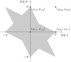
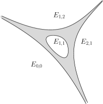
Figure 1. The coamoeba (left) and the amoeba with its complement components $E_{\nu}$ (right) for the polynomial $P(z,w)=z^{2}w-4zw+zw^{2}+1$.

Since $\mathscr{A}_{V}$ is a closed subset of $\mathbb{R}^{n}$, the complement $\mathbb{R}^{n}\setminus\mathscr{A}_{V}$ is open. It consists of a finite number of connected components $E_{i}$, which are convex [12, Section 6.1]. The structure of $\mathbb{R}^{n}\setminus\mathscr{A}_{V}$ can be read from the Newton polytope $\Delta_{P}$ of a polynomial $P,$ i.e. the convex hull in $\mathbb{R}^{n}$ of the list of exponents of terms present in $P$. Recall that the dual cone at a point $\nu\in\Delta_{P}$ to $\Delta_{P}$ is

$$C^{\vee}_{\nu}(\Delta_{P})=\{s\in\mathbb{R}^{n}:\langle s,\nu\rangle=\max_{\alpha\in\Delta_{P}}\langle s,\alpha\rangle\}.$$

A recession cone $C(E)$ of the convex set $E$ is the maximal cone that can be put inside $E$ by a translation.

The following theorem is a summary of Propositions 2.4, 2.5 and 2.6 in [8].

Theorem 2.

There exists an injective order mapping

$$\textup{ord}:\{E\}\to\Delta_{f}\cap\mathbb{Z}^{n}$$

such that the dual cone $C^{\vee}_{\nu}(\Delta_{P}),$ $\nu=\textup{ord}(E)$, is the recession cone of $E$.

So the theorem states that one can encode a component $E$ of the complement $\mathbb{R}^{n}\setminus\mathscr{A}_{V}$ as $E_{\nu}$, where $\nu\in\Delta_{P}\cap\mathbb{Z}^{n}$ and $\nu=\textup{ord}(E).$ We refer readers to Fig. 1 to observe this correspondence for the hypersurface defined by $P(z,w)=z^{2}w-4zw+zw^{2}+1$. Its Newton polytope $\Delta_{P}$ is the convex hull in $\mathbb{R}^{2}$ of points $(0,0)$, $(1,2)$, $(1,1)$ and $(2,1)$.

The order mapping ord can be defined in terms of the Ronkin function $\mathcal{N}_{P}:\mathbb{R}^{n}\to\mathbb{R}$, that is the mean value integral

(1) $$\mathcal{N}_{P}(x)=\frac{1}{(2\pi i)^{n}}\int\limits_{\mathop{\mathrm{Log}}\nolimits^{-1}(x)}\log\big{|}P(z_{1},\ldots,z_{n})\big{|}\frac{dz_{1}\wedge\ldots\wedge dz_{n}}{z_{1}\cdot\ldots\cdot z_{n}},$$

where $x=(x_{1},\ldots,x_{n})\in\mathbb{R}^{n}$. It is affine linear in a component $E$ of the complement $\mathbb{R}^{n}\setminus\mathscr{A}_{V}$. Moreover, the gradient $\left.\textup{grad}\,\mathcal{N}_{P}\right|_{E}$ is equal to $\textup{ord}(E)$ [13].

We define a toric cycle in $(\mathbb{C}^{\times})^{n}\setminus V$ related to $E_{\nu}$ to be an $n$-dimensional real torus

$$\Gamma_{\nu}=\textup{Log}^{-1}(x)=\{z:|z_{1}|=e^{x_{1}},\ldots,|z_{n}|=e^{x_{n}}\},$$

$x=(x_{1},\ldots,x_{n})\in E_{\nu}$. Since $E_{\nu}$ is convex, it contains the segment $[x;y]$ for any pair $x,y\in E_{\nu}$. It follows $\Gamma_{\nu}(y)-\Gamma_{\nu}(x)=\partial\,\textup{Log}^{-1}[x;y]$, and so $\Gamma_{\nu}(x)$ is homologically equivalent to $\Gamma_{\nu}(y)$, therefore we drop $x$ in notation of $\Gamma_{\nu}$.

3. Harnack polynomials and their amoebas

An amoeba is a closed but non-compact subset of $\mathbb{R}^{n}$. Nevertheless, amoebas in $\mathbb{R}^{2}$ have finite areas. Moreover, M. Passare and H. Rullgård showed in [10] that

$$Area(\mathscr{A}_{P})\leq\pi^{2}Area(\Delta_{P})$$

for a bivariate polynomial $P(z,w)$.

Definition 3 ([11]).

A polynomial $P:\mathbb{C}^{2}\to\mathbb{C}$ is called Harnack if its Newton polygon $\Delta_{P}$ has a non-zero area, and the area of its amoeba is maximal, i.e.

(2) $$Area(\mathscr{A}_{P})=\pi^{2}Area(\Delta_{P}).$$

Note that G. Mikhalkin showed in [14] that for a given lattice polygon $\Delta$ one can construct a polynomial $P(z,w)$ with $\Delta_{P}=\Delta$, such that equality (2) holds. The amoeba depicted in Fig. 1 belongs to the Harnack polynomial $P(z,w)=z^{2}w-4zw+zw^{2}+1$.

At first glance, this notion looks to be far from geometry. However, the next statement shows its interactions with the real topology.

Theorem 4 (Mikhalkin-Rullgård [15]).

Let the Newton polygon $\Delta_{P}$ of a polynomial $P(z,w)$ have a non-zero area. Then the following three conditions are equivalent:

1. The amoeba $\mathscr{A}_{P}$ has maximal area.

2. There are constants $a,b,c\in\mathbb{C}^{\times}$ such that $aP(bz,cw)$ has real coefficients. The logarithmic mapping $\mathop{\mathrm{Log}}\nolimits:V\to\mathbb{R}^{2}$ is at most two-to-one, where $V=P^{-1}(0)\cap(\mathbb{C}^{\times})^{2}$.

3. There are constants $a,b,c\in\mathbb{C}^{\times}$ such that $aP(bz,cw)$ has real coefficients. The corresponding real algebraic curve is a Harnack curve for the polygon $\Delta_{P}$.

Point out the properties of amoebas of Harnack polynomials that are important in our study.

Lemma 1.

Given a Harnack polynomial $P(z,w)$ with real coefficients, let $E_{\nu}$ be a component of the complement $\mathbb{R}^{2}\setminus\mathscr{A}_{V}$. Then the image $\mathop{\mathrm{Arg}}\nolimits\circ\mathop{\mathrm{Log}}\nolimits^{-1}(\partial E_{\nu})$ consists of a single point $(\varphi_{\nu},\psi_{\nu})$ from the set

$$\Theta=\{(0,0),\,(0,\pi),\,(\pi,0),\,(\pi,\pi)\}.$$

Proof.

Consider a Harnack polynomial $P(z,w)$ and the complex curve $V$ in $(\mathbb{C}^{\times})^{2}$ defined by $P$. The boundary $\partial\mathscr{A}_{V}$ of its amoeba consists of fold critical points of the projection $\left.\textup{Log}\right|_{V}:V\to\mathscr{A}_{V}$. For each point on the boundary $\partial\mathscr{A}_{V}$, its preimage by $\left.\textup{Log}\right|_{V}$ is a point, while for a point in the interior of $\mathscr{A}_{V}$ the preimage consists of two points.

Now suppose that $(x_{0},y_{0})$ is a point on the boundary $\partial E_{\nu}$ of a component $E_{\nu}$. Then the real torus $\textup{Log}^{-1}(x_{0},y_{0})$ intersects the curve $V$ in a unique point $(z_{0},w_{0})$.

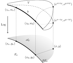
Figure 2. Illustration to the proof of Lemma 1.

The polynomial $P$ has real coefficients by the hypothesis, so that the complex conjugate $(\overline{z}_{0},\overline{w}_{0})$ of the point $(z_{0},w_{0})$ lies on $V$ also. The logarithmic projection $\left.\textup{Log}\right|_{V}:V\to\mathscr{A}_{V}$ maps the conjugate to the same point $(x_{0},y_{0})$ on the boundary $\partial E_{\nu}$. Thus, the points $(z_{0},w_{0})$ and $(\overline{z_{0}},\overline{w_{0}})$ coincide. The point $(z_{0},w_{0})$ is real, and $\mathop{\mathrm{Arg}}\nolimits\circ\mathop{\mathrm{Log}}\nolimits^{-1}(x_{0},y_{0})$ is a point $(\varphi_{0},\psi_{0})$ in $\Theta$.

Assume that $(x_{\nu},y_{\nu})=\mathop{\mathrm{Log}}\nolimits(z_{\nu},w_{\nu})$ is a point on $\partial E_{\nu}$ such that the point $\mathop{\mathrm{Arg}}\nolimits\circ\mathop{\mathrm{Log}}\nolimits^{-1}(x_{\nu},y_{\nu})$ belongs to $\Theta\setminus\{(\varphi_{0},\psi_{0})\}$. We shall show that this leads to a contradiction.

Consider a continuous path $b:[0;1]\to V$ from $b(0)=(z_{0},w_{0})$ to $b(1)=(z_{\nu},w_{\nu})$ such that $b([0;1])=V\cap\mathop{\mathrm{Log}}\nolimits^{-1}[(x_{0},y_{0});(x_{\nu},y_{\nu})]$, where $[(x_{0},y_{0});(x_{\nu},y_{\nu})]$ is an arc on $\partial E_{\nu}$ bounded by $(x_{0},y_{0})$ and $(x_{\nu},y_{\nu})$. At least one of functions $\mathop{\mathrm{Re}}\nolimits z\circ b$, $\mathop{\mathrm{Re}}\nolimits w\circ b$ has values of different signs at $t=0$ and $t=1$. To be definite, assume that $(\mathop{\mathrm{Re}}\nolimits z\circ b)(0)\cdot(\mathop{\mathrm{Re}}\nolimits z\circ b)(1)$ is negative. So there is $\tilde{t}_{0}\in(0;1)$ with $\mathop{\mathrm{Re}}\nolimits z(b(\tilde{t}_{0}))=0$, i.e. a point $(x_{1},y_{1})$ which lifts to the point $(0,w_{1})=b(t_{0})$ on $V$. However, $V$ is defined as a zero locus of $P$ in $(\mathbb{C}^{\times})^{2}$. This contradiction completes the proof. ∎

The four marked points $(\varphi_{\nu},\psi_{\nu})$ on Fig. 1 exhaust the family $\Theta$ for the Harnack polynomial $P(z,w)=z^{2}w-4zw+zw^{2}+1$.

When $P$ is a normalized Harnack polynomial, that is a Harnack polynomial with real coefficients and some special condition (see [11] for a definition), M. Passare in [11] gave an explicit formula for amoeba-to-coamoeba mapping

$$\mathop{\mathrm{Arg}}\nolimits\circ\mathop{\mathrm{Log}}\nolimits^{-1}(x,y)=\left(\pm\pi\frac{\partial\mathcal{N}_{P}}{\partial y}(x,y),\mp\pi\frac{\partial\mathcal{N}_{P}}{\partial x}(x,y)\right),$$

which proves Lemma 1 in the corresponding case.

In general, one has

Lemma 2.

Given a Harnack polynomial $P(z,w)$, let $E_{\nu}$ be a component of the complement $\mathbb{R}^{n}\setminus\mathscr{A}_{V}$. Then the image $\mathop{\mathrm{Arg}}\nolimits\circ\mathop{\mathrm{Log}}\nolimits^{-1}(\partial E_{\nu})$ is a single point $(\varphi_{\nu},\psi_{\nu})$.

Proof.

By Theorem 4 there exist $a,b,c\in\mathbb{C}^{\times}$ such that $\widetilde{P}(z,w)=aP(bz,cw)$ has real coefficients. Applying Lemma 1 to $\widetilde{P}(z,w)$ one gets that the image of $\partial\widetilde{E}_{\nu}$, where $\widetilde{E}_{\nu}$ is the component of $\mathbb{R}^{2}\setminus\mathscr{A}_{\widetilde{P}}$, by the map $\mathop{\mathrm{Arg}}\nolimits\circ\mathop{\mathrm{Log}}\nolimits^{-1}$ is a point from $\Theta$.

Multiplication by a non-zero constant $a$ does not affect the zero locus $\widetilde{V}$ of the polynomial $\widetilde{P}$. The linear transformation $(z,w)\mapsto(bz,cw)$ induces a translation of $\mathscr{A}_{\widetilde{P}}$ by a vector $(\log|b|,\log|c|)$ and a translation of $\mathscr{A}^{\prime}_{\widetilde{P}}$ by $(\arg(b),\arg(c))$. So $\mathop{\mathrm{Arg}}\nolimits\circ\mathop{\mathrm{Log}}\nolimits^{-1}(\partial E_{\nu})$ is a point in $\Theta+(\arg(b),\arg(c))$. ∎

4. Proof of the main result

Let $\overline{\mathbb{C}^{2}}=\mathbb{C}^{2}\cup\{\infty\}$, and $L=L_{1}\cup L_{2}$ be the union of two lines $\{z=0\}$ and $\{w=0\}$ in $\mathbb{C}^{2}=\mathbb{C}_{z}\times\mathbb{C}_{w}$. Since $\overline{\mathbb{C}^{2}}$ is homeomorphic to the sphere $S^{4}$, refer to $\overline{\mathbb{C}^{2}}$ as the spherical compactification of $\mathbb{C}^{2}$. Futher, we denote by $\overline{X}$ the closure in $\overline{\mathbb{C}^{2}}$ of $X\subset\mathbb{C}^{2}$.

Since $(\mathbb{C}^{\times})^{2}\setminus V=\mathbb{C}^{2}\setminus(V\cup L)=\overline{\mathbb{C}^{2}}\setminus\overline{V\cup L},$ one has

$$H_{2}((\mathbb{C}^{\times})^{2}\setminus V)=H_{2}(\overline{\mathbb{C}^{2}}\setminus\overline{V\cup L}).$$

Next, by the Alexander-Pontryagin duality [16], $H_{2}(\overline{\mathbb{C}^{2}}\setminus\overline{V\cup L})\cong H_{1}(\overline{V\cup L}).$ Thus,

$$H_{2}((\mathbb{C}^{\times})^{2}\setminus V)\cong H_{1}(\overline{V\cup L}).$$

Note that $\overline{V\cup L}$ is homeomorphic to the topological sum of three Riemann surfaces defined by $P(z,w)=0$, $z=0$ and $w=0$ with certain points identified (see Fig. 3).

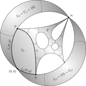
Figure 3. Illustration to the proof of the main theorem.

Recall that the family $\{\Gamma_{\nu}\}$ consists of toric cycles in $(\mathbb{C}^{\times})^{2}\setminus V$ associated with components $E_{\nu}$ of the complement $\mathbb{R}^{2}\setminus\mathscr{A}_{V}$. We are going to construct a family of 1-cycles $\sigma_{\nu}$ in $\overline{V\cup L}$ dual to the family $\{\Gamma_{\nu}\}$ in the folowing sense

(3) $$\textup{link}(\sigma_{\mu},\Gamma_{\nu})=\pm\delta_{\mu\nu}=\begin{cases}0,\,&\text{if $\mu\neq\nu$},\\ \pm 1,\,&\text{if $\mu=\nu$}.\end{cases}$$

Existence of the family $\{\sigma_{\nu}\}$ with such property of pairing implies, obviously, homological independence of the families $\{\Gamma_{\nu}\}$ and $\{\sigma_{\nu}\}$.

By Lemma 2 we know that the image $\mathop{\mathrm{Arg}}\nolimits\circ\mathop{\mathrm{Log}}\nolimits^{-1}(\partial E_{\nu})$ is a single point $(\varphi_{\nu},\psi_{\nu})$. Therefore we can define the lifting of $\partial E_{\nu}$ to the curve $V$ as

$$\tau_{\nu}=\{(e^{x+i\varphi_{\nu}},e^{y+i\psi_{\nu}}):(x,y)\in\partial E_{\nu}\}\subset(\mathbb{C}^{\times})^{2},$$

that is $\tau_{\nu}=V\cap\mathop{\mathrm{Log}}\nolimits^{-1}(\partial E_{\nu})$. Now, we need to construct compact cycles $\sigma_{\nu}$ in $\overline{V\cup L}$ using $\tau_{\nu}$.

Consider the boundary $\partial\tau_{\nu}=\overline{\tau}_{\nu}\setminus(\mathbb{C}^{\times})^{2}$ of the lifting in $\overline{\mathbb{C}^{2}}$. Its cardinality may be $0$, $1,$ or $2$. For instance, when $E_{\nu}$ is a bounded component, $\partial\tau_{\nu}$ is empty. In this case, we put $\sigma_{\nu}=\tau_{\nu}$.

Let $E_{\nu}$ be an unbounded component. The set $\partial\tau_{\nu}$ consists of one or two points in the ray $\overline{\{t(e^{i\varphi_{\nu}},0):t\geq 0\}}\subset\overline{L_{2}}$ or in the ray $\overline{\{t(0,e^{i\psi_{\nu}}):t\geq 0\}}\subset\overline{L_{1}}$.

The particular configuration of points in $\partial\tau_{\nu}$ depends on the recession cone $C(E_{\nu})$ of the component $E_{\nu}$. Since $C(E_{\nu})$ is a sector (possibly degenerated to a ray), its position in $\mathbb{R}^{2}$ can be described by the pair $(u,v)\in T^{2}=S^{1}\times S^{1}$, where $S^{1}$ is the unit circle. In other words, all the possible shapes of $E_{\nu}$ can be identified with a subset on the torus $T^{2}$. (In some sense, $T^{2}$ is the configurational space of components $E_{\nu}$).

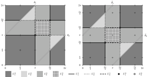
Figure 4. Partition (4) of the torus $T^{2}$. Components $U_{j}^{i}$ are given in local coordinates $0\leq\theta_{1},\theta_{2}<2\pi$ (left; the angles $\theta_{1}$, $\theta_{2}$ are measured from the horizontal coordinate axis in $\mathbb{R}^{2}$ to the vectors $u,v$ counter-clockwise) and $0\leq\tilde{\theta}_{1},\tilde{\theta}_{2}<2\pi$ (right; the angles $\tilde{\theta}_{1}$, $\tilde{\theta}_{2}$ are measured from the diagonal of the positive quadrant in $\mathbb{R}^{2}$ to the vectors $u,v$ counter-clockwise). Cuts $|\theta_{2}-\theta_{1}|=\pi$ (or $|\tilde{\theta}_{2}-\tilde{\theta}_{1}|=\pi$) corresponds to the degeneration of the Newton polytope $\Delta_{P}$.

In order to describe constructions of $\sigma_{\nu}$ for all the possible shapes of $E_{\nu}$, we consider the partition of the torus

(4) $$T^{2}=U_{1}^{0}\sqcup U_{2}^{0}\sqcup U_{1}^{1}\sqcup U_{2}^{1}\sqcup U_{3}^{1}\sqcup U_{1}^{2}\sqcup U_{2}^{2}\sqcup U_{3}^{2}\sqcup U_{4}^{2},$$

where components $U_{j}^{i}$ are defined as in Fig. 4. Table 1 establishes the correspondence between components $U_{j}^{i}$ of the partition, possible sets $\partial\tau_{\nu}$ and constructions of the cycle $\sigma_{\nu}$. The construction of $\sigma_{\nu}$ involves the lifting $\tau_{\nu}$ and segments $l_{z}(a,b)$, $l_{w}(a,b)$ in the closure of the rays $\{t(e^{i\varphi_{\nu}},0):t\geq 0\}\subset\overline{L_{2}}$, $\{t(0,e^{i\psi_{\nu}}):t\geq 0\}\subset\overline{L_{1}}$. The segments $l_{z}(a,b)$, $l_{w}(a,b)$ join points (possibly infinite) $a,b$ on the corresponding rays. We denote by $p_{i}$ points in $\overline{V}\cap L_{2}$, by $q_{j}$ points in $\overline{V}\cap L_{1}$ and by $O$ the origin $(0,0)$.

For example, $U_{2}^{0}$ consists of two points, each encoding the same recession cone generated by $(-1,0)$ and $(0,-1)$. Thus, $\partial\tau_{\nu}$ consists of two points $p\in\overline{V}\cap L_{2}$ and $q\in\overline{V}\cap L_{1}$, and to construct $\sigma_{\nu}$ one need to add $l_{z}(O,p)$ and $l_{w}(O,q)$ to $\tau_{\nu}$. (See Fig. 3).

Table 1. The correspondence between components $U_{j}^{i}$ of the partition (4), possible sets $\partial\tau_{\nu}$ and constructions of the cycle $\sigma_{\nu}$.

component of $T^{2}$	$\partial\tau_{\nu}$	construction of $\sigma_{\nu}$
$U_{1}^{2}$	$\{\infty\}$	$\tau_{\nu}\cup\{\infty\}$
$U_{2}^{2}$	$\{\infty\}$	$\tau_{\nu}\cup\overline{(l_{z}(O,\infty)\cup l_{w}(O,\infty))}$
$U_{3}^{2}$	$\{O,\infty\}$	either $\tau_{\nu}\cup\overline{l_{z}(O,\infty)}$
		or $\tau_{\nu}\cup\overline{l_{w}(O,\infty)}$
$U_{4}^{2}$	$\{O\}$	$\tau_{\nu}\cup\{O\}$
$U_{1}^{1}$	either $\{p,\infty\}$	$\tau_{\nu}\cup\overline{l_{z}(p,\infty)}$
	or $\{q,\infty\}$	$\tau_{\nu}\cup\overline{l_{w}(q,\infty)}$
$U_{2}^{1}$	either $\{p,\infty\}$	$\tau_{\nu}\cup l_{z}(O,p)\cup\overline{l_{w}(O,\infty)}$
	or $\{q,\infty\}$	$\tau_{\nu}\cup l_{w}(O,q)\cup\overline{l_{z}(O,\infty)}$
$U_{3}^{1}$	either $\{O,p\}$	$\tau_{\nu}\cup l_{z}(O,p)$
	or $\{O,q\}$	$\tau_{\nu}\cup l_{w}(O,q)$
$U_{1}^{0}$	either $\{p_{1},p_{2}\}$	$\tau_{\nu}\cup l_{z}(p_{1},p_{2})$
	or $\{q_{1},q_{2}\}$	$\tau_{\nu}\cup l_{w}(q_{1},q_{2})$
$U_{2}^{0}$	$\{p,q\}$	$\tau_{\nu}\cup l_{z}(O,p)\cup l_{w}(O,q)$

Let us write the left-hand side of (3)

$$\textup{link}(\sigma_{\mu},\Gamma_{\nu})=\textup{ind}(h_{\mu},\Gamma_{\nu})$$

as the intersection index in $\overline{\mathbb{C}^{2}}$ of the cycle $\Gamma_{\nu}$ and the $2$-dimensional chain

$$h_{\mu}=\{(e^{x+i\varphi_{\mu}},e^{y+i\psi_{\mu}}):(x,y)\in E_{\mu}\}\cup\sigma_{\mu},$$

such that $\partial h_{\mu}=\sigma_{\mu}.$ The toric cycle $\Gamma_{\nu}$ has the form $\mathop{\mathrm{Log}}\nolimits^{-1}(x,y)$, where $(x,y)\in E_{\nu}$. So the chain $h_{\mu}$ does not intersect $\Gamma_{\nu}$ if $\mu\neq\nu$. Meanwhile, if $\mu=\nu$ the cycle $\Gamma_{\nu}$ intersects $h_{\mu}$ in a single point $(e^{x+i\varphi_{\nu}},e^{y+i\psi_{\nu}})$. Therefore, $\textup{ind}(h_{\nu},\alpha(\Gamma_{\mu}))=\pm\delta_{\nu\mu}$. Q.E.D.

Acknowledgments

The first author was financed by the grant of the President of the Russian Federation for state support of leading scientific schools NSh-9149.2016.1. The second author was supported by the grant of the Russian Federation Government for research under supervision of leading scientist at Siberian Federal University, contract №14.Y26.31.0006.

References

- [1] Poincaré, H.: Sur les résidus des intégrales doubles. Acta Math. 9, 321–380 (1887)
- [2] Leray, J.: Le calcul différentiel et intégral sur une variété analytique complexe. (Problème de Cauchy. III.) Bull. Soc. Math. de France 87, 81–180 (1959)
- [3] Tsikh, A., Yger, A.: Residue currents. J. Math. Sci. 120:6, 1916-1971 (2004)
- [4] Aizenberg, L.A., Yuzhakov, A.P.: Integral representations and residues in multidimensional complex analysis. Amer. Math. Soc., Providence, RI (1983)
- [5] Gelfond, O.A., Khovanskii, A.G.: Toric geometry and Grothendieck residues. Mosc. Math. J. 2:1, 99–112 (2002)
- [6] Mkrtchian, M., Yuzhakov, A.: The Newton polytope and the Laurent series of rational functions of variables. (Russian) Izv. Akad. Nauk ArmSSR 17, 99-105 (1982)
- [7] Forsberg, M.: Amoebas and Laurent series. Doctoral thesis, KTH Stockholm (1998)
- [8] Forsberg, M., Passare, M., Tsikh, A.: Laurent determinants and arrangements of hyperplane amoebas. Adv. in Math. 151, 45-70 (2000)
- [9] Bushueva, N.A., Tsikh, A.K.: On amoebas of algebraic sets of higher codimension. Proc. Steklov Inst. Math. 279, 52-63 (2012)
- [10] Passare, M., Rullgård, H.: Amoebas, Monge-Ampère measures, and triangulations of the Newton polytope. Preprint, Stockholm University, (2000)
- [11] Passare, M.: The Trigonometry of Harnack Curves. Journal of Sib. Federal Univeristy. Math. & Physics 9, 347-352 (2016)
- [12] Gelfand, I., Kapranov, M., Zelevinsky, A.: Discriminants, Resultants and Multidimentional Determinants. Bikhäuser, Boston (1994)
- [13] Rullgård, H.: Topics in geometry, analysis and inverse problems. Doctoral thesis, Stockholm University, (2003)
- [14] Mikhalkin, G.: Real algebraic curves, the moment map and amoebas. Ann. of Math. 151, 309-326 (2000)
- [15] Mikhalkin, G., Rullgård, H.: Amoebas of maximal area. Internat. Math. Res. Notices 9, 441-451 (2001)
- [16] Aleksandrov, P.S.: Topological duality theorems. I: Closed sets. Amer. Math. Soc. Transl. 30:2 (1963)