Extremely large magnetoresistance and Kohler’s rule in PdSn₄: a complete study of thermodynamic, transport and band structure properties.

Abstract

The recently discovered material PtSn₄ is known to exhibit extremely large magnetoresistance (XMR) that also manifests Dirac arc nodes on the surface. PdSn₄ is isostructure to PtSn₄ with same electron count. We report on the physical properties of high quality single crystals of PdSn₄ including specific heat, temperature and magnetic field dependent resistivity and magnetization, and electronic band structure properties obtained from angle resolved photoemission spectroscopy (ARPES). We observe that PdSn₄ has physical properties that are qualitatively similar to those of PtSn₄, but find also pronounced differences. Importantly, the Dirac arc node surface state of PtSn₄ is gapped out for PdSn₄. By comparing these similar compounds, we address the origin of the extremely large magnetoresistance in PdSn₄ and PtSn₄; based on detailed analysis of the magnetoresistivity, $\rho(H,T)$, we conclude that neither carrier compensation nor the Dirac arc node surface state are primary reason for the extremely large magnetoresistance. On the other hand, we find that surprisingly Kohler’s rule scaling of the magnetoresistance, which describes a self-similarity of the field induced orbital electronic motion across different length scales and is derived for a simple electronic response of metals to applied in a magnetic field is obeyed over the full range of temperatures and field strengths that we explore.

I Introduction

The recent discovery of three-dimensional topological semi-metals generated lots of attention. Topological semi-metals can be classified as three different types:Armitage et al. a Dirac semimetal, a Weyl semimetal, and a nodal-line semimetal. A Dirac semimetal has points in the Brillouin zone where doubly degenerate conduction and valence bands are touching linearly, and has been realized in Na₃Bi and Cd₃As₂.Liu et al. (2014); Wang et al. (2013) A Weyl semimetal is similar to Dirac semimetal, but a Weyl semi-metal exhibits Weyl points that are crossing of singly degenerate electronic bands, which requires the breaking of either time-reversal or inversion symmetry. Weyl points have chirality which is represented by the sign of the determinant for the velocity tensor.Weng et al. (2016) Experimental manifestations of Weyl semimetals are: TaAs, NbAs, TaP and transition metal dichalcogenides including WTe₂ .Lv et al. (2015); Xu et al. (2015a, b, c); Wu et al. (2016a) A nodal-line semimetal has a gap closing along a line in the Brillouin zone instead of at isolated points. Several materials have experimentally confirmed to be nodal-line semimetals: PbTaSe₂, ZrSiS and TlTaSe₂.Bian et al. (2016a); Schoop et al. (2016); Bian et al. (2016b) A different type of a novel topological quantum structure was identified recently in PtSn₄ which has a Dirac node arc feature on the surface, whose (topological) origin is still unknown.Wu et al. (2016b) In the bulk, PtSn₄ is a metallic with a number of complex electron and hole Fermi surface sheets containing significant carrier densities.Wu et al. (2016b)

The fascinating physical properties of PtSn₄ were reported in Ref. Mun et al., 2012. Most importantly, it manifests an extremely large magnetoresistance (XMR) of $\sim$ 10${}^{5}\,\%$ for $T\,=\,1.8$ K and $H\,=\,140$ kOe, without any evidence of saturation.Mun et al. (2012) In the following years, many of other topological materials that also showed XMR have been found.

Several mechanisms have been suggested for such XMR in various materials. Nearly perfect electron-hole compensation has been suggested as the origin of XMR ($\sim\,10^{5}\,\%$ at 4.5 K and 147 kOe) in WTe₂.Ali et al. (2014) (Although it has also been noted that in this material there is a clear relation between MR and the residual resistivity ratio, $\rho_{0}$)Ali et al. (2015). Magnetic field induced changes in Fermi surface structure have been suggested as the cause of XMR in NbSb₂ ($\sim\,10^{5}\,\%$ at 2 K and 9 T) and Cd₃As₂ ($\sim\,10^{5}\,\%$ at 5 K and 9 T), specifically field induced gaps in Dirac points or splitting of Dirac Fermi points into separated Weyl points.Ali et al. (2014); Liang et al. (2015) More recently, for the case of LaSb ($\sim\,10^{6}\,\%$ at 2 K and 9 T) and LaBi ($\sim\,10^{5}\,\%$ at 2 K and 9 T) XMR has been associated with $d$-$p$ orbital mixing.Tafti et al. (2016a, b) Despite all of these possible mechanisms, the origins of XMR in all of these materials are open to debate.

PdSn₄ is isostructural to PtSn₄;Kubiak and Wolcyrz (1984); Nylén et al. (2004) it has an orthorhombic structure and a space group number of 68, with Pd and Sn each having a unique crystallographic site.Nylén et al. (2004) The lattice parameters of PdSn₄ are $a\,=\,6.4417\,\AA$, $b\,=\,11.4452\,\AA$ and $c\,=\,6.3886\,\AA$, which are very similar to those of PtSn₄: $a\,=\,6.418\,\AA$, $b\,=\,11.366\,\AA$ and $c\,=\,6.384\,\AA$.Nylén et al. (2004); Künnen et al. (2000) Since not only the structure, but also the electron count is same, the primary difference between PdSn₄ and PtSn₄ may be the spin orbit coupling strength. Therefore, it is interesting to compare these two materials.

In this paper, we report the physical properties of PdSn₄, including temperature and the magnetic field dependent transport and magnetic properties as well as a detailed angle resolved photoemmision spectroscopy (ARPES) and density functional theory (DFT) study of its electronic bulk and surface band structure. Compared to PtSn₄, the anisotropic physical properties of PdSn₄ are qualitatively similar. In contrast, our ARPES results show that whereas PtSn₄ exhibits a Dirac node arc at the surface, the corresponding surface state is clearly gapped out in PdSn₄. We rule out a number of proposed microscopic mechanisms for XMR, through detailed analysis of the magnetoresistivity and band structure. In particular, we show that carrier compensation cannot explain XMR in PtSn₄ and PdSn₄. In addition, we point out a surprising scaling property of the magnetoresistivity that follows Kohler’s rule over a wide magnetic field and temperature range, revealing to a robust scale invariance of the electronic orbital motion known from classical descriptions of magnetotransport.

II experimental and theoretical methods

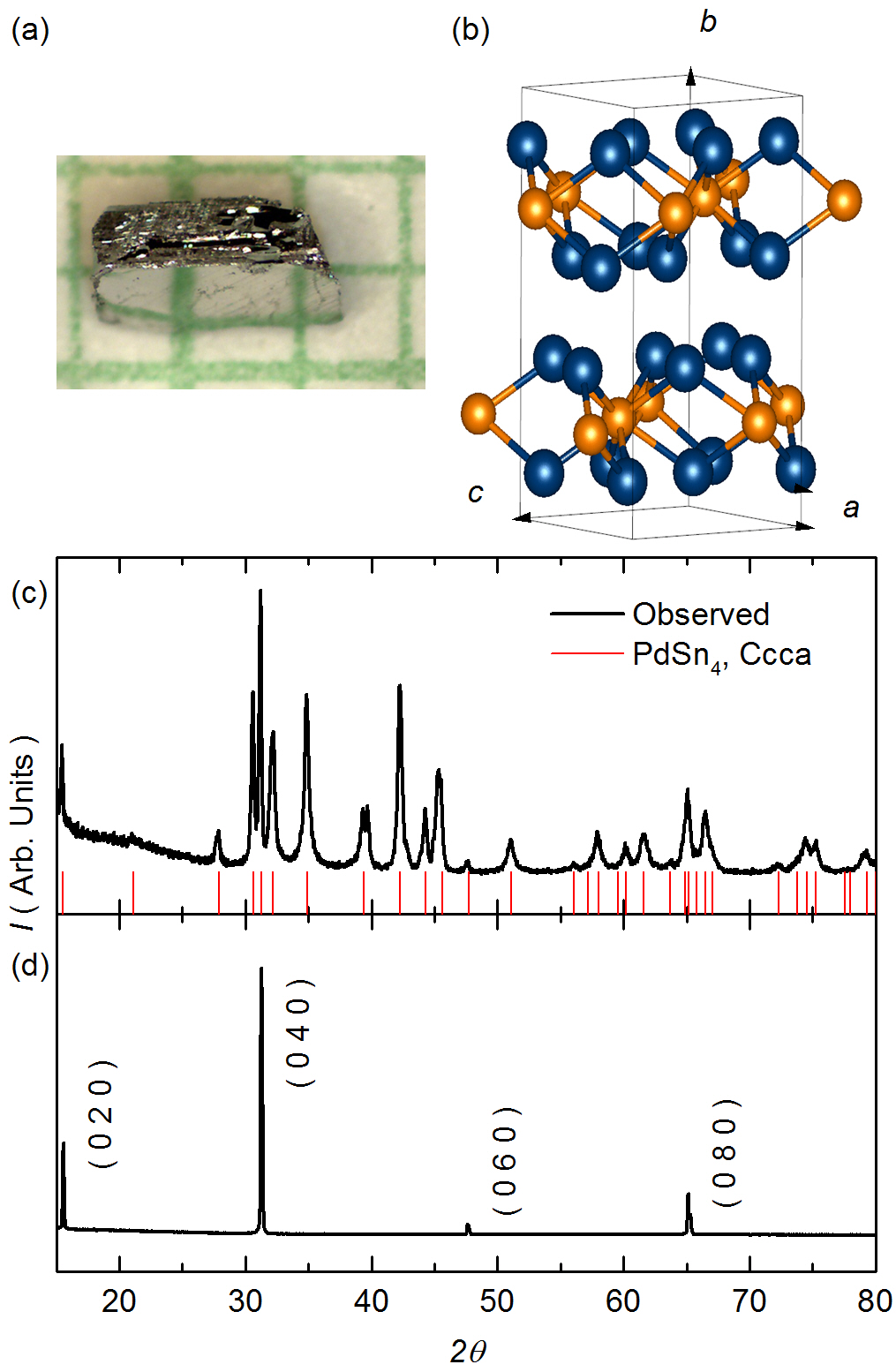
Figure 1: (color online) (a) Single crystal of PdSn₄. (b) Crystal structure (Pd: orange sphere, Sn: blue sphere). (c) Powder X-ray diffraction pattern (Black lines) and reported PdSn₄ ($Ccca$) peaks from ref.Nylén et al. (2004) (Red lines). (d) Single crystal X-ray diffraction pattern identifying the (0 h 0) lines.

Single crystals of PdSn₄ were grown out of Sn-rich binary melts.Okamoto (2000) We put an initial stoichiometry of Pd₂Sn₉₈ into a fritted alumina crucible [CCS],Canfield et al. (2016) and then sealed in it into an amorphous silica tube under partial Ar atmosphere. The ampoule was heated up to 600  over 5 hours, held there for 5 hours, rapidly cooled to 325   and then slowly cooled down to 245  over more than 100 hours, and then finally decanted using a centrifuge.Canfield and Fisk (1992) The fritted crucible allowed for the clean separation of crystals from the Sn flux.Petrovic et al. (2012) The single crystalline sample has a clear plate like shape with mirrored surface and typical dimension of $\sim$ 2 mm $\times$ 1 mm $\times$ 0.3 mm.(Fig. 1 (a))

A Rigaku MiniFlex diffractometer (Cu $K_{\alpha 1,2}$ radiation) was used for acquiring x-ray diffraction (XRD) data at room temperature (Fig. 1 (c)). All the peak positions are well matched with the reported orthorhombic PdSn₄ structure.Nylén et al. (2004) However, the relative intensity of the peaks is different from the calculated powder pattern, presumably preferential orientation of the ground powder due to the layered structure. The crystal structure in real space is shown in Fig. 1 (b). The crystallographic $b$-axis is anticipated to be perpendicular to the mirrored surface shown in Fig. 1 (a). To confirm this, we did single crystal XRD.Jesche et al. (2016) When the x-ray beam is incident perpendicular to the surface, only (0 k 0) peaks were observed as shown in Fig. 1 (d). This confirms that the crystallographic $b$ direction is perpendicular to the mirrored surface shown in Fig. 1 (a).

Temperature and field dependent transport properties were measured in a Quantum Design(QD), Physical Property Measurement System for 1.8 $\leq T\leq$ 300 K and $\left|H\right|\leq$  140 kOe. The contacts for the electrical transport measurement were prepared in a standard four-probe configuration using Epotek-H20E silver epoxy. The magnetization as a function of temperature and field was measured in a QD, Magnetic Property Measurement System for 1.85 $\leq T\leq$ 300 K and $H\leq$ 70 kOe. A modified QD sample rotating platform with an angular resolution of 0.1 $\deg$ was used for angular-dependent dc magnetization measurements.

ARPES measurements were carried out using a laboratory-based tunable VUV laser ARPES system, consisting of a Scienta R8000 electron analyzer, picosecond Ti:Sapphire oscillator and fourth harmonic generator.Jiang et al. (2014) All Data were collected with a constant photon energy of 6.7 eV. Angular resolution was set at $\sim$ 0.05^∘ and 0.5^∘ (0.005 Å^-1 and 0.05  Å^-1) along and perpendicular to the direction of the analyzer slit (and thus cut in the momentum space), respectively; and energy resolution was set at 1 meV. The size of the photon beam on the sample was $\sim$30 $\mu$m. Samples were cleaved in situ at a base pressure lower than $1\times 10^{-10}$ Torr. Samples were cleaved at 40 K and kept at the cleaving temperature throughout the measurement.

Band structure with spin-orbital coupling (SOC) in density functional theory (DFT)Hohenberg and Kohn (1964); Kohn and Sham (1965) have been calculated with PBEPerdew et al. (1996) exchange-correlation functional, a plane-wave basis set and projected augmented wave methodBlöchl (1994) as implemented in VASP5,6.Kresse and Furthmüller (1996, 1996) For bulk band structure of PdSn₄, we used the conventional orthorhombic cell of 20 atoms with a Monkhorst-PackMonkhorst and Pack (1976) (8 $\times$ 6 $\times$ 8) $k$-point mesh including the $\Gamma$ point and a kinetic energy cutoff of 251 eV. The convergence with respect to $k$-point mesh was carefully checked, with total energy converged below 1 meV/atom. Experimental lattice parameters have been used with atoms fixed in their bulk positions. A tight-binding model based on maximally localized Wannier functionsMarzari and Vanderbilt (1997); Souza et al. (2001); Marzari et al. (2012) was constructed to reproduce closely the bulk band structure including SOC in the range of $E_{F}\,\pm\,1$ eV with Pd $s$ and $d$ orbitals and Sn $s$ and $p$ orbitals. Then Fermi surface and spectral functions of a semi-infinite PdSn₄ (0 1 0) surface were calculated with the surface Green’s function methodsLee and Joannopoulos (1981a, b); Sancho et al. (1984, 1985) as implemented in WannierTools.Wu et al.

The PtSn₄ data that are shown here for comparison are from our previous paper on PtSn₄.Mun et al. (2012)

III Results and analysis

III.1 Specific heat

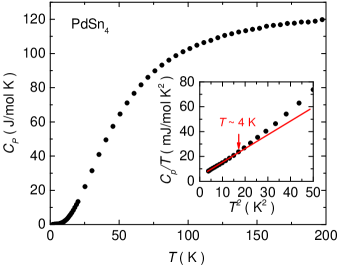
Figure 2: (color online) Temperature dependent specific heat, $C_{P}$, of PdSn₄. Inset shows $C_{p}/T$ as a function of $T^{2}$. The red line is a linear fit to the lowest temperature PdSn₄ data.

The temperature dependent specific heat, $C_{P}$, of PdSn₄, shown in Fig. 2, does not show any signature of a phase transition. We plot the $C_{P}/T$ as a function of $T^{2}$ in the inset to Fig. 2 to infer the electronic specific heat coefficient, $\gamma$, and the Debye temperature, $\Theta_{D}$. This is based on the relation $C_{P}\,=\,\gamma T+\beta T^{3}$ at low temperature; $\gamma\,=\,4$ mJ/mol K² and $\Theta_{D}\,\sim\,206$ K. These values are very similar to those of PtSn₄ ($\gamma\,\sim\,4$ mJ/mol K² and $\Theta_{D}\,\sim\,210$ K).Mun et al. (2012) Since both systems have $\gamma$ values of less than 1 mJ/mol K² atom, neither has a significant density of states at the Fermi surface or strong electron correlations.

III.2 Resistivity

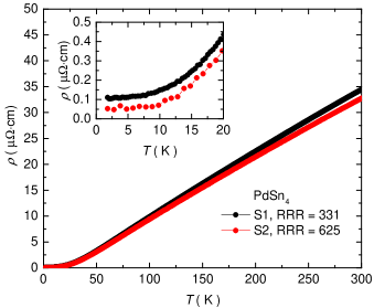
Figure 3: (color online) Temperature dependent resistivity of two PdSn₄ single crystals.

Figure 3 shows the temperature dependent resistivity, $\rho(T)$, measured from 1.8 K to 300 K. The current was applied perpendicular to the crystallographic $b$ direction. (i.e. within the plane of the plate-like sample). Sample S1 has a residual resistivity ratio (RRR = $\rho(300\,\textrm{ K})/\rho(1.8\,\textrm{K})$) value of 331, and sample S2 has RRR = 625. In both cases, the large RRR indicates the high quality of the crystals. The overall behavior of $\rho(T)$ is metallic, which is similar to PtSn₄.Mun et al. (2012) It shows almost linear temperature dependence at high temperatures; the low temperature ($T\,<\,10$ K) data from S1 and S2 were fitted with a polynomial function, $\rho\,(\textrm{T})\,=\,\rho_{0}+AT^{2}$. The obtained values are $\rho_{0}\,=\,0.105\,\mu\Omega\,\textrm{cm}$ and $A\,=\,2.7\,\times\,10^{-4}\,\mu\Omega\,\textrm{cm}/\textrm{K}^{2}$ for S1, and $\rho_{0}\,=\,0.049\,\mu\Omega\,\textrm{cm}$ and $A\,=\,2.2\,\times\,10^{-4}\,\mu\Omega\,\textrm{cm}/\textrm{K}^{2}$ for S2. Given that S2 has RRR, $\rho_{0}$ and $A$ values closer to those reported for PtSn₄ than S1,Mun et al. (2012) we chose to use S2 to carry out further transport experiments with the applied magnetic field.

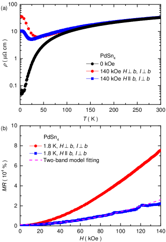
Figure 4: (color online) (a) Temperature dependent resistivity of PdSn₄ in zero applied magnetic field (black filled circles), and in 140 kOe for different magnetic field directions; red filled circles ($H\,\perp\,b$, $H\,\perp\,I$) and blue filled squares ($H\,\parallel\,b$, $H\,\perp\,I$). (b) Magnetoresistance (MR) of PdSn₄ at 1.8 K for different magnetic field and current directions; red filled circles ($H\,\perp\,b$, $H\,\perp\,I$), blue filled squares ($H\,\parallel\,b$, $H\,\perp\,I$). Magenta dashed-line is fitted line based on a two-band model (see text).

The $\rho(T)$ of PdSn₄ for $H\,=\,140$ kOe was measured from 1.8 K to 300 K with the two different magnetic field directions (red filled circles for $H\,\perp\,b$ and blue filled squares for $H\,\parallel\,b$) (Fig. 4 (a)). Note that the current was always applied in an $I\,\perp\,b$ and $I\,\perp\,H$ direction. The current thus always flows in the $a$-$c$ plane, perpendicular to the applied magnetic field. For comparison, we also plotted the $\rho(T)$ of PdSn₄ for $H\,=\,0$ kOe (black filled circles). For both field directions, PdSn₄ shows a strong field dependence at low temperatures. To be more specific, a local minimum is observed near 40 K ($H\,\perp\,b$) and 25 K ($H\,\parallel\,b$), followed by steep increases in resistivity that tends to saturate as $T\,\rightarrow\,2$ K.

Transverse magnetoresistance (MR) measurements were carried out from 0 Oe to 140 kOe at 1.8 K, with MR defined as $(\rho(H)-\rho(H=0))\times\,100/\rho(H=0)$. The magnetic field dependency of MR in both directions is quadratic rather than linear, and there is no evidence of saturation in MR up to 140 kOe. Anomalies in the higher magnetic field regime are due to quantum oscillations. (see discussion below). The order of the MR at 140 kOe is 10${}^{4}\,\%$ which is extremely large.

As suggested by Fig. 4 (a), the MR shown in Fig. 4 (b) shows a clear anisotropy between the two different field directions: at 140 kOe, MR = 7.5 $\times\,10^{4}$ $\%$ for $H\,\perp\,b$ and MR = 2.4 $\times\,10^{4}$ $\%$ for $H\,\parallel\,b$. It is interesting that both PtSn₄ and PdSn₄ show a larger MR when the magnetic field is applied perpendicular to the $b$ direction (i.e. within the basal plane). This is in contrast to many layered materials with large MR anisotropy that manifest the largest MR when the magnetic field is applied perpendicular to the plane.Zhao et al. (2015); Eto et al. (2010) Furthermore, for layered materials that manifest quasi-two dimensional Fermi surfaces, it has been predicted that the transverse MR along one magnetic field direction (perpendicular to the plane) increases quadratically while it tends to saturate for a field that lies within the plane.Lifshits et al. (1973) Given the quadratic MR, for both field directions, found for PdSn₄ as well as PtSn₄, it seems that the magetotransport is dominated by 3D Fermi surface (FS) sheets, even though each compound cleaves and exfoliates well.

III.3 Hall coefficient

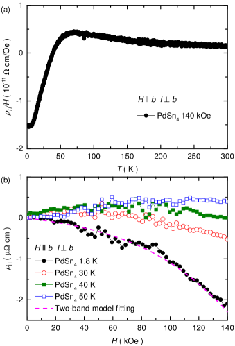
Figure 5: (color online) (a) Temperature dependent Hall resistivity divided by the applied magnetic field, $\rho(H)/H$, of PdSn₄ for $H\,=\,140\,kOe$ $\parallel\,b$. (b) magnetic field dependent Hall resistivity of PdSn₄ at 1.8 K, 30 K, 40 K, and 50 K. The dashed magenta line is based on a two-band model (see text).

Electron-hole compensation can be a reason for large MR and has been invoked in the case of WTe₂.Ali et al. (2014) In general, the conductivity tensor components $\sigma_{xy}$ and $\sigma_{yx}$ are proportional to 1/$H$ when the carrier density of electrons and holes are not approximately equal (i.e. $n_{e}\,\gg\,n_{h}$ or $n_{e}\,\ll\,n_{h}$). Then the diagonal components of resistivity tensors, except $\rho_{zz}$, saturate as the magnetic field goes to infinity. On the other hand, the resistivity tensor components $\rho_{xx}$ and $\rho_{yy}$ increase quadratically without saturating at high field when $n_{e}\,\approx\,n_{h}$ since $\sigma_{xy}$ and $\sigma_{yx}$ are then dominated by higher order of $1/H$ terms. One should note that this is true only if the following assumptions are fulfilled: (i) there are closed trajectories and (ii) in the high field regime.Lifshits et al. (1973) In order to see whether such a compensation senario is possible for PdSn₄, we measured its Hall resistivity, $\rho_{H}$. In Fig. 5 (a), the temperature-dependent Hall coefficient, $R_{H}\,=\,\rho_{H}/H$, of PdSn₄ at 140 kOe from 1.8 K to 300 K is plotted. Above 65 K, $R_{H}$ of PdSn₄ shows monotonic behavior with a positive value which indicates that hole-like carriers dominate its transport properties. $R_{H}$ of PdSn₄ starts to decrease rapidly below 65 K, crosses $R_{H}\,=\,0$ at 38 K, and then saturates to $R_{H}\,\approx\,-1.5\,\times\,10^{-11}$ Ω cm/Oe below 7 K. Given that $R_{H}$ changes sign at low temperatures, it is tempting to associate this phenomenon with perfect carrier compensation. However, this assumes that the mobilities of all carrieres are equal. This is because $R_{H}$ is not only a function of carrier density but also mobility. Therefore, we need a way to disentangle the carrier density and mobility contributions to $R_{H}$.

One indication of compensation is a nonlinear behavior of $\rho_{xy}(H)\,\equiv\,\rho_{H}$ in high magnetic fields.Lifshits et al. (1973) Thus, we measured the $\rho_{H}$ of PdSn₄ as a function of the magnetic field in Fig. 5 (b). The $\rho_{H}$ of PdSn₄ shows nonlinear behavior in the low temperature regime, where it shows non-saturating, large MR. This means PdSn₄ has very similar values of carrier densities, i.e. $n_{e}\,\approx\,n_{h}$, whereas the mobility of electrons is larger compared to the mobility of holes based on $R_{H}(T)$ at low temperature (see Fig. 5 (a)).

We were able to use a simplified two-band model to fit the $\rho_{H}(H)$ and MR data at 1.8 K in order to do a quantitative analysis.Pippard (1989) This method has been successfully used in many materials.Rullier-Albenque et al. (2009, 2010); Luo et al. (2015)

$${\rho}_{xx}\left(B\right)=\frac{1}{e}\frac{\left({n}_{h}{\mu}_{h}+{n}_{e}{\mu}_{e}\right)+\left({n}_{h}{\mu}_{e}+{n}_{e}{\mu}_{h}\right){\mu}_{h}{\mu}_{e}{B}^{2}}{{\left({n}_{h}{\mu}_{h}+{n}_{e}{\mu}_{e}\right)}^{2}+{\left({n}_{h}{-n}_{e}\right)}^{2}{{\mu}_{h}}^{2}{{\mu}_{e}}^{2}{B}^{2}}$$ (1)

$${\rho}_{xy}\left(B\right)=\frac{B}{e}\frac{\left({n}_{h}{{\mu}_{h}}^{2}{-n}{{}_{e}{\mu}_{e}}^{2}\right)+\left({n}_{h}-{n}_{e}\right){{\mu}_{h}}^{2}{{\mu}_{e}}^{2}{B}^{2}}{{\left({n}_{h}{\mu}_{h}+{n}_{e}{\mu}_{e}\right)}^{2}+{\left({n}_{h}{-n}_{e}\right)}^{2}{{\mu}_{h}}^{2}{{\mu}_{e}}^{2}{B}^{2}}$$ (2)

The values obtained from the two-band model are $n_{e}=1.6\times 10^{27}\text{m}^{-3}\pm 0.1\times 10^{27}\text{m}^{-3}$, $n_{h}=1.5\times 10^{27}\text{m}^{-3}\pm 0.1\times 10^{27}\text{m}^{-3}$ such that their ratio is $c=n_{h}/n_{e}=0.93\pm 0.02$. The mobilities are found to be $\mu_{e}=0.34\pm 0.04$ m²/V s and $\mu_{h}=0.27\pm 0.03$ m²/V s such that their ratio is $c_{\mu}=\mu_{h}/\mu_{e}=0.80\pm 0.05$. The corresponding $R^{2}$-values of the fit are very good $R^{2}-1=0.02$, showing that although the Fermi surface clearly consists of several hole and electron pockets with different mobilities and effective masses (see more below), the resistivity can be well captured (at least qualitatively) within a two-band model. We want to emphasize that the simplified two-band model equations above are based on the assumption of (i) only one electron and one hole band are present, (ii) the isotropic free electron gas model is applicable, and (iii) components of the conductivity tensor that contain $z$ need not be considered. In addition, we have found that slightly worse but still reasonable fits can be obtained with other mobility ratios $c_{\mu}$ and total densities $n_{e}$. The data constrains the ratio $c$ more than the value of $n_{e}$.com

The best fits we have obtained are plotted in both Fig. 4 (b) and Fig. 5 (b) with magenta dashed lines. Unlike PtSn₄,Mun et al. (2012) the values of $n_{e}$ and $n_{h}$ for PdSn₄ obtained from the fit are very similar, within about 7 $\%$ of each other, whereas $\mu_{e}\,>\,\mu_{h}$, which was expected from the Hall data at the high magnetic fields. The shape of $\rho_{xy}$ immediately yields two constraints $(i)n_{e}\mu_{e}^{2}>n_{h}\mu_{h}^{2}$ and $n_{h}<n_{e}$, which follows directly from the fact that the linear and cubic coefficients in an expansion $\rho_{xy}=a_{1}B+a_{3}B^{3}$ both need to be negative $a_{1},a_{3}<0$. From the fact that the non-linearity sets in around $B_{2}\approx 8$T, we can further derive the relation $(1-cc_{\mu}^{2})(1+cc_{\mu})^{2}/[cc_{\mu}^{2}(1-c)(1+c_{\mu})^{2}]\approx B_{2}^{2}\mu_{e}^{2}$.

III.4 Magnetization

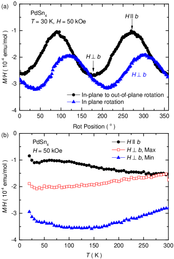
Figure 6: (color online) (a) Angular-dependent magnetic susceptibility of PdSn₄ in both in-plane to out-of-plane rotation and in-plane rotation at $T\,=\,30$ K and $H\,=\,50$ kOe. (b) Temperature-dependent magnetic susceptibility of PdSn₄ at 50 kOe, $H\,\parallel\,b$ (black filled circles), $H\,\perp\,b$ for maximal in-plane magnetization orientation (red open rectangles) and $H\,\perp\,b$ for minimal in-plane magnetization orientation (blue filled triangles).

Both out-of-plane and in-plane angular dependent magnetization measurements are shown in Fig. 6 (a). The observed magnetic properties of PdSn₄ are diamagnetic in all directions with a clear anisotropy between the $a$-$c$ plane and the $b$ direction. The data are taken at 30 K and 50 kOe, but the magnetization is linear as a function of the magnetic field for $H\,\leq\,7$ T, so the angular dependent magnetic susceptibilities measured in different magnetic fields of 25 kOe, 50 kOe and 70 kOe are the same. On the other hand, both angular dependent magnetic susceptibility show deviations from simple sine function behavior when the temperature is below 30 K due to quantum oscillations.

Based on the angular dependent magnetization measurements, we find that the maximum susceptibility (smallest negative value) occurs for $H\,\parallel\,b$. For $H\,\perp\,b$, we find a simple angular variation of $M(\theta)$ and can identifiy an in-plane field orientation that produces a minimal and maximal response separated by 90^o. In Fig. 6 (b) we present the temperature dependence magnetization from 20 K to 300 K with 50 kOe along the three different magnetic field directions. All of them show weak temperature dependence, and the anisotropy gets smaller as temperature is increased. The low temperature upturn is due to entering the temperature range of quantum oscillations (see below).

In order to understand the physical meaning of an anisotropic susceptibility, it is important to separate core diamagnetism from Pauli paramagnetism and Landau diamagnetism. If we subtract the core diamagnetic contribution,Boudreaux and Mulay (1976); Bain and Berry (2008) we can infer the conduction electron contribution to the magnetic susceptibility. Even after the core diamagnetic correction, $\chi_{core}\,=\,-1.05\,\times\,10^{-4}$ emu/mol of PdSn₄,Boudreaux and Mulay (1976); Bain and Berry (2008) the remaining conduction electron susceptibility is still essentially diamagnetic. Based on an equation for the total electronic susceptibility of a metalBlundell (2001)

$$\chi={\chi}_{P}\left[1-\frac{1}{3}{\left(\frac{{m}_{e}}{{m}^{*}}\right)}^{2}\right],$$ (3)

where $m_{e}$ is an electron mass, m^∗ is an effective mass and $\chi_{P}$ is Pauli paramagetism, the result indicates that the carriers should have rather low effective masses.

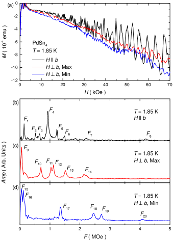
Figure 7: (color online) (a) Magnetization isotherms of PdSn₄ without background subtraction for $H\,\parallel\,b$, $H\,\perp\,b$, Max and $H\,\perp\,b$, Min at 1.85 K. (b) FFT spectra of dHvA data for $H\,\parallel\,b$. (c) FFT spectra of dHvA data for $H\,\perp\,b$, Max. (d) FFT spectra of dHvA data for $H\,\perp\,b$, Min.

More detailed information about the Fermi surface and effective masses can be obtained via measurement and analysis of quantum oscillations. Thus, we measured the magnetization of PdSn₄ as a function of the magnetic field, $M(H)$, up to 70 kOe at 1.85 K in all three salient directions: $H\,\parallel\,b$, $H\,\perp\,b$, Max and $H\,\perp\,b$, Min as shown in Fig. 7 (a). Note that the plotted magnetization data are raw data without subtracting the background of the sample rotator, but clear de Haas van Alphen (dHvA) oscillations are readily detected. For analysis, the oscillatory part of the magnetization is obtained as a function of $1/B$ after subtracting a linear background. We then used a fast fourier transform (FFT) algorithm. The FFT data are shown in Fig. 7 (b) for $H\,\parallel\,b$, Fig. 7 (c) for $H\,\perp\,b$, Max and Fig. 7 (d) for $H\,\perp\,b$, Min. All the frequencies are labeled on the figures and listed in the Table 1. $F_{\textrm{14}}$ is broad, and it might be a superposition of the second harmonics of $F_{\textrm{11}}$ and $F_{\textrm{12}}$. In addition, $F_{\textrm{19}}$ is likely a second harmonic of $F_{\textrm{17}}$. Here, we note that Shubnikov-de Haas oscillation show some low frequencies ($F_{1}$, $F_{2}$ and $F_{3}$) for $H\,\parallel\,b$ as noted in Fig. 4 (b), but these oscillations are much clearer in the $M(H)$ data. The corresponding extremal areas were calculated via the the Onsager relation which gives a direct proportionality between frequency and extremal area, $F_{\textrm{i}}=\frac{\hbar c}{2\pi e}S_{i}$.

Table 1: Frequencies of the peaks from Fig. 7 (b)-(d) and Fig. 8 (c), corresponding orbital areas $S_{i}\,=\,2\,\pi\,e\,F_{i}/(\hbar\,c)$, and effective masses from Fig. 8

								Rotator												Plastic disk
$H\,\parallel\,b$								$H\,\perp\,b$, Max						$H\,\perp\,b$, Min						$H\,\perp\,b$
		MOe		$\AA^{-2}$		me				MOe		$\AA^{-2}$				MOe		$\AA^{-2}$				MOe		$\AA^{-2}$		me
$F_{1}$		0.14		0.0013				$F_{9}$		0.06		0.00057		$F_{15}$		0.06		0.00057		$F^{*}_{9}$		0.06		0.00057		0.03
$F_{2}$		0.52		0.0050		0.07		$F_{10}$		0.70		0.0067		$F_{16}$		0.11		0.0011		$F^{*}_{10}$		0.76		0.0073		0.05
$F_{3}$		0.65		0.0062		0.08		$F_{11}$		1.04		0.0099		$F_{17}$		1.34		0.0128		$F^{*}_{11}$		1.06		0.0101		0.05
$F_{4}$		0.94		0.0090		0.09		$F_{12}$		1.12		0.0107		$F_{18}$		2.46		0.0235
$F_{5}$		1.23		0.0118		0.08		$F_{13}$		1.51		0.0144		$F_{19}$		2.72		0.0260		$F^{*}_{13}$		1.57		0.015		0.05
$F_{6}$		1.47		0.0140		0.08		$F_{14}$		2.13		0.0203		$F_{20}$		4.09		0.0391		$F^{*}_{14}$		2.13		0.0203		0.06
$F_{7}$		2.20		0.0210		0.104
$F_{8}$		4.18		0.0399		0.106

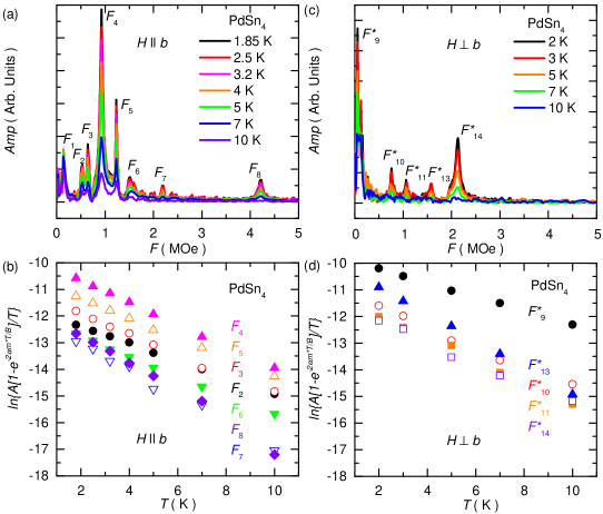
Figure 8: (color online) (a) Temperature dependence of the fast Fourier transformed dHvA data of PdSn₄ for $H\,\parallel\,b$ and $T$ = 1.85 K, 2.5 K, 3.2 K, 4 K, 5 K, 7 K, 10 K. (b) Mass plot of dHvA orbits at each frequency when the magnetic field was applied parallel to the crystallographic $b$-axis. (c) Temperature dependence of the fast Fourier transformed dHvA data of PdSn₄ for $H\,\perp\,b$ and $T$ = 2 K, 3 K, 5 K, 7 K, 10 K. (d) Mass plot of dHvA orbits at each frequency when the magnetic field was applied perpendicular to the crystallographic $b$-axis.

$M(H)$ data were measured not only at the base temperature, 1.85 K, but also at the several other temperatures, 2.5 K, 3.2 K, 4 K, 5 K, 7 K and 10 K. (Fig. 8) For the measurement of these magnetic isotherms, the sample was mounted on a diamagnetic, isotropic, amorphous disk and manually rotated with respect to the applied field. Exactly the same peaks that we detected from rotator (Fig. 7 (b)) are found when the $H\,\parallel\,b$. On the other hand, the FFT data for $H\,\perp\,b$ show slightly different peaks compared to both $H\,\perp\,b$, Max and $H\,\perp\,b$, Min measured from the rotator, although the frequency of the peaks are very similar to that of $H\,\perp\,b$, Max, except for $F_{12}$.

Figure. 8 shows that the oscillation amplitudes decrease as temperature increases. The Lifshitz-Kosevich formulaShoenberg (1984) explains a phase smearing which is related to amplitude. Specifically, the effect of temperature is described by

$${R}_{T}=\frac{\alpha{m}^{*}T/H}{\sinh(\alpha{m}^{*}T/H)}$$ (4)

where $\alpha=2\pi^{2}ck_{B}/e\hbar$. We used an average value for $1/H\,=\,(1/H_{min}+1/H_{max})*1/2$, where $H_{min}$ and $H_{max}$ indicate the range of the data, we used for FFT. Effective masses are obtained based on the above equation, and linear behavior in mass plot in Fig. 8 (b) and (d) suggests that the obtained effective masses are reasonable. The effective mass of each frequency is shown in the Table. 1. All effective masses are small and approximately equal to each other. However, the low frequency peak, $F^{*}_{9}$ has a particularly small effective mass which suggests a potentially large contribution to density of states. Thus, the carriers confined to the Fermi surface related to the $F^{*}_{9}$ may give a dominant contribution to the anisotropy of the magnetic susceptibility.

IV Discussion and comparison to PtSn₄

The temperature and field dependent properties, including anisotropies, of PdSn₄ are qualitatively similar to those of PtSn₄,Mun et al. (2012) but there exist some important quantitative differences. The question that we now would like to address is whether a comparison of these two, related, materials help us understand the origin of XMR.

IV.1 Carrier compensation

Carrier compensation is one of the reasons that many materials, including WTe₂,Ali et al. (2014) LaBi,Tafti et al. (2016b) LaSbTafti et al. (2016b) and PtBi₂Gao et al. (2017), are thought to exhibit XMR behavior. However, the scenario of nearly perfect compensation of carriers cannot explain XMR in PdSn₄ and PtSn₄. At the simplest level, PdSn₄ exhibits a larger degree of compensation than PtSn₄ but shows a smaller, MR. At low temperatures where MR is large, PdSn₄ shows a non-linear field dependence of $\rho_{H}(H)$ at high field whereas a linear $\rho_{H}$ is observed for PtSn₄ in the high field regime.Mun et al. (2012) Note that such non-linear behavior is an indication of carrrier compensation. Moreover, the results from classical two-band-model fitting indicate that PdSn₄ has similar electron and hole carrier densities albeit with different mobilities, whereas PtSn₄ has an almost two order of magnitude difference between electron and hole carrier densities.Mun et al. (2012) (It should be noted, though, that if we consider classical carrier compensation theory, this describes the non-saturating $H^{2}$ behavior but not the prefactor.)Lifshits et al. (1973) This means that, in this simplest treatment, the magnitude of MR cannot be explained. For the more specific case of WTe₂ an exitonic insulator was invoked;Ali et al. (2014) for PdSn₄ and PtSn₄ such an insulating state is unlikely given their multiple and complex Fermi surfaces. Finally, a recent theoretical paper studied the compensated Hall effect in confined geometry with electron-hole recombination near the edge, inducing a large MR.Alekseev et al. (2017) In this case, linear response regime is found when the edge currents dominate the resistance.Alekseev et al. (2017) On the other hand, for PdSn₄ and PtSn₄ we find quadratic behavior up to 140 kOe. We can thus confidently rule out (i) carrier compensation, (ii) the emergence of an excitonic insulating state, and (iii) MR enhancement by sample confinement as the primary origins of XMR in PdSn₄ and PtSn₄.

IV.2 Dirac arc node feature

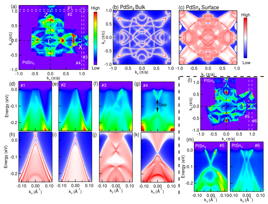
Figure 9: Experimental ARPES and calculated results for the electronic Fermi surface and band dispersion of PdSn₄. (a) Fermi-surface plot of ARPES intensity integrated within 10 meV of the chemical potential along $\Gamma-Z$ and $\Gamma-X$. (b) Bulk FS calculated by density functional theory (DFT) at $k_{y}=0.364~{}\pi/b$. (c) Calculated surface FS. (d)-(g) ARPES band dispersions along cut #1-#4 in (a), respectively. (h)-(k) Calculated surface band dispersion corresponding to (d)-(g). (l) For comparison, Fermi-surface plot of ARPES intensity integrated within 10 meV of the chemical potential along $\Gamma-Z$ and $\Gamma-X$ in PtSn₄.Wu et al. (2016b) (m) Band dispersion in PtSn₄ at $k_{x}=0.88\text{ and }1.0~{}\pi/a$ along cut #5 and 6 in (l).Wu et al. (2016b)

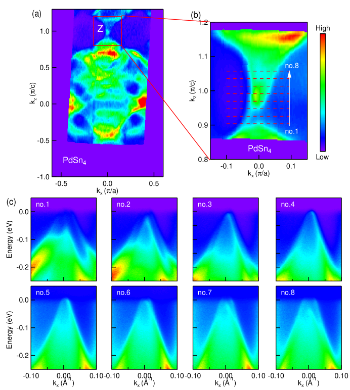
Figure 10: Fermi surface and band dispersion in the proximity of the Z point,(0,1), of PdSn₄. (a) Fermi surface plot of the ARPES intensity integrated within 10 meV of the chemical potential along $\Gamma-Z$. (b) Zoomed image of the red box in (a), red dashed lines mark cuts no.1 –- no.8. (c) Band dispersion along cuts no. 1 –- no. 8. Cut no. 5 passes through the Z point.

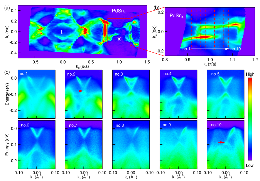
Figure 11: Fermi surface plot and band dispersion close to the X point, (1,0), of PdSn₄. (a) Fermi surface plot of the ARPES intensity integrated within 10 meV of the chemical potential along $\Gamma-X$. (b) Zoomed image of the red box in (a), red dashed lines mark cuts no.1 – no.10. (c) Band dispersion along cuts no.1 –- no.10. Cut no. 6 passes through the X point.

In order to check whether the Dirac arc node feature seen in PtSn₄Wu et al. (2016b) can be associated with XMR in PdSn₄, or not, angle resolved photo emission spectroscopy (ARPES) measurements and surface band structure calculations were performed. The Fermi surface and band dispersion along key directions in the Brillouin Zone (BZ) for PdSn₄ are shown in Fig. 9. Panel (a) shows the ARPES intensity integrated within 10 meV about the chemical potential. High intensity areas mark the contours of the FS sheets. The FS consists of at least two electron pockets at the center of BZ surrounded by several other electron and hole FS sheets. Fig. 9 (b) shows the calculated bulk FS, which matches the ARPES data well close to the center of the zone in Fig. 9 (a). However, it does not predict the linear band dispersion near the $Z$ point (see below) or the FS crossings close to the $X$ point, missing a set of curved FS sheets that are present in Fig. 9 (a). This is similar to the results of PtSn₄, where a surface state calculation was needed to reproduced the Fermi surface sheets in the proximity of the $X$ point.Wu et al. (2016b) Thus we carried out a surface spectral function calculation as shown in Fig. 9 (c) and we can clearly see extra FS sheets connecting the bands close to the center of BZ and at the $X$ point. Band dispersion along several cuts in proximity of the $Z$ and $X$ points are shown in Figs. 9 (d)–(g). Close to the $Z$ point (Figs. 9 (d) and (e)), the dispersion resembles a Dirac-like feature. This linear dispersion was not found in bulk calculations and only appeared in the surface spectral function calculations (Figs. 9 (h) and (i)). The small gap in the Dirac-like feature at the Z point (Figs. 9 (e) and (i)) is reduced to zero for cuts further away from the BZ boundary (Figs. 9 (d) and (h)). Close to the $X$ point [Fig. 9 (f)], the band dispersion consists of Dirac-like dispersion (surface origin) surrounded by broad hole bands (most likely bulk states). The data agree well with surface spectral function calculation shown in Fig. 9 (j). In Fig. 9 (g), the observed conduction band and valence band have a significant band gap as marked by the black arrows, which is in agreement with the surface spectral function calculation shown in Fig. 9 (k).

The data in Figs. 9 (a), (d)–(g) demonstrate that the experimentally observed band structure has both bulk and surface components, and the Dirac-like features near Z and X points have surface origin. Compared to the results of PtSn₄ shown in Fig. 9 (l), the Fermi surface of these two compounds are very similar close to the zone center, which is consistent with the similar crystal structures and electronic configurations of the compounds. However, comparing the results in Figs. 9 (f) and (g) with those in Figs. 9 (m), the primary difference between these two data sets is that for PdSn₄, the double Dirac node arcs surface state is gapped out [Fig. 9 (g)].

In Fig. 10, we show details of the features of PdSn₄ near the Z point. An enlarged image from the red box in Fig. 10(a) is shown in panel (b), where two triangular-shaped FS sheets make a somewhat disconnected hourglass like shape. The detailed evolution of band dispersions along cuts no. 1 to no. 8 is shown in Fig. 10(c). A sharp linear dispersion (the inner band) starts to cross at a binding energy of $\sim$100 meV in cut no. 1; this band moves up in energy and eventually becomes almost degenerate with the outer bands in cut no. 5. As we move further toward the second BZ cuts(no. 6 – no. 8), the sharp band moves back down in energy, as expected.

A similar study of the band evolution near the X point is shown in Fig. 11. We focus on the Fermi surface and band dispersion in a small area in the part of the BZ that is marked by the red box in Fig. 11(a). The Fermi surface in this region consists of two parabolic FS sheets intersecting each other, forming two almost parallel straight segments in the overlapping region. Detailed band dispersion along cuts no. 1 to no. 10 are shown in Fig. 11(c). The data along cut no. 1 show a sharp electron band enclosed by the bulk intensity. As we move to cut no.2, a Dirac-like dispersion is revealed with the possible Dirac point marked by the red arrow. Moving closer to the X point (cut no. 3), we can see a gap develops between the conduction and valence bands, and another electron band emerges. As we move to cuts no. 4, 5, and 6, the two electron bands come closer and eventually merge together in cut no. 6 at the X point. A significant gap between the conduction and valence bands persists across these cuts. The gap size slowly decreases and seems to form another Dirac dispersion in cut no. 10 in the second BZ. The observed features around X point are markedly different for PtSn₄,Wu et al. (2016b) where gapless Dirac node arc structure is observed.

Even though, in PdSn₄ the Dirac point at $Z$ is a surface state and the Dirac arc node feature is gapped out, XMR behavior is still present in both compounds. Moreover, both PdSn₄ and PtSn₄ show larger MR when the magnetic field is applied perpendicular to the $b$ direction. This is not consistent with the measured surface states at a surface perpendicular to $b$ giving rise to the measured XMR, because the resulting orbits do not lie in the surface plane.

IV.3 Kohler’s rule

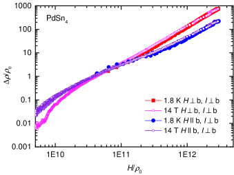
Figure 12: (color online) Kohler’s plot of PdSn₄ magnetoresistance data. Red filled squares are based on $\rho(H)$ data taken at 1.8 K.($H\,\perp\,b$, $I\,\perp\,b$) Magenta open squares are based on $\rho(T)$ data taken under the magnetic field of 140 kOe. ($H\,\perp\,b$, $I\,\perp\,b$) Blue filed circles are based on $\rho(H)$ data taken at 1.8 K.($H\,\perp\,b$, $I\,\parallel\,b$) Purple open circles are based on $\rho(T)$ data taken under the magnetic field of 140 kOe.($H\,\perp\,b$, $I\,\parallel\,b$)

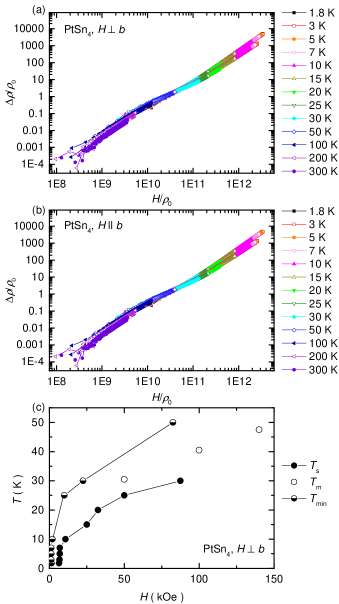
Figure 13: (color online) Kohler’s plot of PtSn₄ magnetoresistance data with various temperatures; 1.8 K, 3 K, 5 K, 7 K, 10 K, 15 K, 20 K, 25 K, 30 K, 50 K, 100 K, 200 K, 300 K with two different magnetic field directions from ref. Mun et al., 2012 (a) $H\,\perp\,b$ and (b) $H\,\parallel\,b$. (c) Temperature-field phase diagram for PtSn₄ for $H\,\perp\,b$. Filled black circles are the starting point of the Kohler’s rule slope change in (a) in the high magnetic field regime. Open black circles are the temperature of the local minimum in $\rho(T)$ data for an applied magnetic field of 50, 100 or 140 kOe. Half filled circles are the shallowest slope in the Kohler’s plot in (a).

Let us now investigate whether a classical description of the electronic motion can give insight into the MR results. The well-known Kohler’s rule states that the change of resistivity $\Delta\rho$, where $\Delta\rho\,=\,\rho(T,H)-\rho_{0}$ and where $\rho_{0}\,\equiv\,\rho(T,H\,=\,0)$, under the magnetic field $H$ can be described as a scaling function of the variable $H\tau$.Ziman (1960) Here, $\tau$ is the mean time between scattering events of conduction electrons, and it is inversely proportional to $\rho_{0}$. Such a scaling behavior expresses a self-similarity of the electronic orbital motion across different length scales: an invariance of the magnetoresponse under the combined transformation of shrinking the orbital length $L\sim 1/H$ by increasing $H$ while at the same time also increase the scattering rate $1/\tau$ by the same factor such that $H\tau$ remains unchanged, indicates that the system behaves identical on different length scales. The formula for the Kohler’s rule can be written as follows with scaling function $F(x)$.

$$\Delta\rho/\rho_{0}\,=\,F(H/\rho_{0})$$ (5)

It should be appreciated that Kohler’s rule is both powerful and simplified; Kohler’s rule scaling breaks down if different scattering mechanisms emerge on different temperature or lengthscales or if Landau orbit quantization plays a role.Pippard (1989)

In Figs. 12 and 13 we plot MR data for PdSn₄ and PtSn₄ respectively, using the scaling ansatz of Eq. (5) that emphasizes the Kohler’s rule behavior found for both of these compounds. In Fig. 12, for PdSn₄ we plot MR data, for two field directions, extracted from two different extremes of MR sweeps: $\rho(T\,=\,1.8$ K, 500 Oe $\leq\,H\,\leq 140$ kOe) and $\rho$(1.8 K $\leq\,T\,\leq\,300$ K, $H\,=\,140$ kOe). Remarkably although the two data sets, lie in very different field and temperature regimes, they fall precisely on top of each other, describing a sigmoidal-shaped curve. These plots demonstrate that the behavior of all of the MR data for PdSn₄, from 1.8 K to 300 K, from 0 Oe to 140 kOe is captured and described by a Kohler’s rule. Figure 13 shows the same generalized Kohler’s plot for MR data collected on PtSn₄.Mun et al. (2012) We find that all of the $\rho(T,500\,\textrm{Oe}\,\leq\,H\,\leq\,140$ kOe) data for temperatures ranging from 1.8 K all the way up to 300 K fall onto similar sigmoidal-shaped curves.

The importance of the such complete MR data collapse in Figs. 12 and 13 cannot be over emphasized. In Fig. 12, for PdSn₄, we find precisely the same behavior at 1.8 K as we so for temperatures ranging up to 300 K. The two very different cuts through $T$-$H$ phase space yield the same Kohler’s rule curve. This means that the behavior of the MR at 1.8 K is governed by the simple physics as the behavior at 300 K; i.e. there is not a “metal-to-insulator” transition or other such feature associated with the local minima in the $\rho(T)$ data for any given applied field. Instead, given that a generalized form of Kohler’s rule describes the PdSn₄ and PtSn₄ data exceptionally well, any features that are seen in the $\rho(T,H)$ data in the low temperature/high field limit originate from the same physics giving rise to the high temperature/low field behavior.

This generalized Kohler’s rule analysis, of course, raises the question of what is the origin of the sigmoidal-shape we find for both PdSn₄ and PtSn₄? In both Figs. 12 and 13 there is a well defined, linear, high field/low temperature (upper right hand corners of the plots) region that can be associated with power law behavior. As either temperature is increased or field is lowered the curvature associated with the sigmoidal-shape appears and grows. It is possible, even likely, given the clear dHvA oscillations, that the high magnetic field (or low temperature) regime is where $\omega_{c}\tau\,>\,1$. Conversely, high temperatures and low magnetic field will be where $\omega_{c}\tau\,<\,1$. It should be noted that large MR can be expected only when $\omega_{c}\tau\,\gg\,1$.Pippard (1989) For both PtSn₄ and PdSn₄ the middle of the sigmoidal region of the curves occur for $\Delta\rho/\rho_{0}\,\sim\,1$; this may provide a physical sense of, or criterion for, $\omega_{c}\tau\,\gg\,1$.

We can use the Kohler’s rule data shown in Fig. 13 (a) to delineate the low temperature/high field part of the $T$-$H$ phase space from the high temperature/low field part. In Fig. 13 (c) we plot data inferred from (i) the deviation from high field/low temperature linear behavior in the upper right part of Fig. 13 (a), and (ii) the position of the inflection point associated with the sigmoidal-shaped curve. These data provide an estimate of the extent of the high field/low temperature region for this specific PtSn₄ sample. We can also use the local minima in the $\rho(T)$ data measured for a constant applied magnetic field to define a set of ($T$,$H$) data points. We include these data in Fig. 13 (c) as well; they clearly are associated with crossing over from a low temperature limit to a high temperature limit in terms of $\omega_{c}\tau$.

The challenge that PdSn₄ and PtSn₄ present is to understand what specific feature of their band structure is responsible for the remarkable size of the MR that is observed. This still unresolved point is what makes research into these compounds, as well as other XMR materials a compelling topic for ongoing research.

V Conclusion

In conclusion, the thermodynamic and transport properties of PdSn₄ are strikingly similar to those of PtSn₄; both compounds have closely related temperature dependent specific heat, anisotropic resistivity and magnetization, although the precise magnitudes of RRR and MR are quantitatively different. We have focused on the origin of XMR in these two materials. Based on our analysis, we can rule out carrier compensation and the surface state Dirac arc node features observed in PtSn₄ can be considered as key reasons for the XMR. Instead, we find that, by using a generalized Kohler’s plot, all of the MR data for both PdSn₄ and PtSn₄ collapse onto simple sigmoidal manifolds. For PdSn₄, the fact that MR data from an isothermal field sweep at 1.8 K and a constant field (140 kOe) temperature sweep from 1.8 K to 300 K fall indistinguishably on top of each other (with similar results for PtSn₄) clearly emphasizes that the behavior of the MR data for these materials is captured by the basic metal physics encoded into Kohler’s rule. A future challenge is to identify the specific property of PdSn₄, PtSn₄ and other XMR compounds that give rise to the remarkable size and durability of the observed XMR.

Note that as we were preparing to submit this work, another paper on PdSn₄ was posted.Xu et al. Single crystals of PdSn₄ were grown out of excess Sn, but instead of separating the crystals from excess Sn by decanting in the liquid state, the excess Sn was allowed to solidify around the PdSn₄ crystals. PdSn₄ crystals were ultimately separated from solidified Sn flux by acid etching. The samples reported in ref. Xu et al., have substantially lower RRR values as well as substantially reduced MR. Although ref. Xu et al., only reports a subset of the quantum oscillation frequencies we were able to detect, the ones that are reported agree with what we found to a large degree. Given the importance of $\rho_{0}$ in the physics described by Kohler’s rule, it is probably preferable to compare PdSn₄ and PtSn₄ samples grown in similar ways and with closer $\rho_{0}$ and RRR values.

References

References

- (1) N. P. Armitage, E. J. Mele, and A. Vishwanath, arXiv:1705.01111 .
- Liu et al. (2014) Z. K. Liu, B. Zhou, Y. Zhang, Z. J. Wang, H. M. Weng, D. Prabhakaran, S.-K. Mo, Z. X. Shen, Z. Fang, X. Dai, Z. Hussain, and Y. L. Chen, Science 343, 864 (2014).
- Wang et al. (2013) Z. Wang, H. Weng, Q. Wu, X. Dai, and Z. Fang, Phys. Rev. B 88, 125427 (2013).
- Weng et al. (2016) H. Weng, X. Dai, and Z. Fang, J. Phys.: Condens. Matter 28, 303001 (2016).
- Lv et al. (2015) B. Q. Lv, N. Xu, H. M. Weng, J. Z. Ma, P. Richard, X. C. Huang, L. X. Zhao, G. F. Chen, C. E. Matt, F. Bisti, V. N. Strocov, J. Mesot, Z. Fang, X. Dai, T. Qian, M. Shi, and H. Ding, Nat. Phys. 11, 724 (2015).
- Xu et al. (2015a) S.-Y. Xu, I. Belopolski, N. Alidoust, M. Neupane, G. Bian, C. Zhang, R. Sankar, G. Chang, Z. Yuan, C.-C. Lee, S.-M. Huang, H. Zheng, J. Ma, D. S. Sanchez, B. Wang, A. Bansil, F. Chou, P. P. Shibayev, H. Lin, S. Jia, and M. Z. Hasan, Science 349, 613 (2015a).
- Xu et al. (2015b) S.-Y. Xu, N. Alidoust, I. Belopolski, Z. Yuan, G. Bian, T.-R. Chang, H. Zheng, V. N. Strocov, D. S. Sanchez, G. Chang, C. Zhang, D. Mou, Y. Wu, L. Huang, C.-C. Lee, S.-M. Huang, B. Wang, A. Bansil, H.-T. Jeng, T. Neupert, A. Kaminski, H. Lin, S. Jia, and M. Zahid Hasan, Nat. Phys. 11, 748 (2015b).
- Xu et al. (2015c) S.-Y. Xu, I. Belopolski, D. S. Sanchez, C. Zhang, G. Chang, C. Guo, G. Bian, Z. Yuan, H. Lu, T.-R. Chang, P. P. Shibayev, M. L. Prokopovych, N. Alidoust, H. Zheng, C.-C. Lee, S.-M. Huang, R. Sankar, F. Chou, C.-H. Hsu, H.-T. Jeng, A. Bansil, T. Neupert, V. N. Strocov, H. Lin, S. Jia, and M. Z. Hasan, Sci. Adv. 1 (2015c).
- Wu et al. (2016a) Y. Wu, D. Mou, N. H. Jo, K. Sun, L. Huang, S. L. Bud’ko, P. C. Canfield, and A. Kaminski, Phys. Rev. B 94, 121113 (2016a).
- Bian et al. (2016a) G. Bian, T.-R. Chang, R. Sankar, S.-Y. Xu, H. Zheng, T. Neupert, C.-K. Chiu, S.-M. Huang, G. Chang, I. Belopolski, D. S. Sanchez, M. Neupane, N. Alidoust, C. Liu, B. Wang, C.-C. Lee, H.-T. Jeng, C. Zhang, Z. Yuan, S. Jia, A. Bansil, F. Chou, H. Lin, and M. Z. Hasan, Nat. Comms. 7, 10556 (2016a).
- Schoop et al. (2016) L. M. Schoop, M. N. Ali, C. Straßer, A. Topp, A. Varykhalov, D. Marchenko, V. Duppel, S. S. P. Parkin, B. V. Lotsch, and C. R. Ast, Nat. Comms. 7, 11696 (2016).
- Bian et al. (2016b) G. Bian, T.-R. Chang, H. Zheng, S. Velury, S.-Y. Xu, T. Neupert, C.-K. Chiu, S.-M. Huang, D. S. Sanchez, I. Belopolski, N. Alidoust, P.-J. Chen, G. Chang, A. Bansil, H.-T. Jeng, H. Lin, and M. Z. Hasan, Phys. Rev. B 93, 121113 (2016b).
- Wu et al. (2016b) Y. Wu, L.-L. Wang, E. Mun, D. D. Johnson, D. Mou, L. Huang, Y. Lee, S. L. Bud’ko, P. C. Canfield, and A. Kaminski, Nat. Phys. 12, 667 (2016b).
- Mun et al. (2012) E. Mun, H. Ko, G. J. Miller, G. D. Samolyuk, S. L. Bud’ko, and P. C. Canfield, Phys. Rev. B 85, 035135 (2012).
- Ali et al. (2014) M. N. Ali, J. Xiong, S. Flynn, J. Tao, Q. D. Gibson, L. M. Schoop, T. Liang, N. Haldolaarachchige, M. Hirschberger, N. P. Ong, and R. J. Cava, Nature 514, 205 (2014).
- Ali et al. (2015) M. N. Ali, L. Schoop, J. Xiong, S. Flynn, Q. Gibson, M. Hirschberger, N. Ong, and R. Cava, EPL (Europhysics Letters) 110, 67002 (2015).
- Liang et al. (2015) T. Liang, Q. Gibson, M. N. Ali, M. Liu, R. J. Cava, and N. P. Ong, Nat. Mater. 14, 280 (2015).
- Tafti et al. (2016a) F. F. Tafti, Q. D. Gibson, S. K. Kushwaha, N. Haldolaarachchige, and R. J. Cava, Nat. Phys. 12, 272 (2016a).
- Tafti et al. (2016b) F. F. Tafti, Q. Gibson, S. Kushwaha, J. W. Krizan, N. Haldolaarachchige, and R. J. Cava, Proc. Natl. Acad. Sci. U.S.A. , 201607319 (2016b).
- Kubiak and Wolcyrz (1984) R. Kubiak and M. Wolcyrz, J. Less Common Met. 97, 265 (1984).
- Nylén et al. (2004) J. Nylén, F. G. Garcia, B. Mosel, R. Pöttgen, and U. Häussermann, Solid State Sci. 6, 147 (2004).
- Künnen et al. (2000) B. Künnen, D. Niepmann, and W. Jeitschko, J. Alloys and Compd. 309, 1 (2000).
- Okamoto (2000) H. Okamoto, Phase Diagrams for Binary Alloys, Desk Handbook (ASM International, Materials Park, OH, 2000).
- Canfield et al. (2016) P. C. Canfield, T. Kong, U. S. Kaluarachchi, and N. H. Jo, Philos. Mag. 96, 84 (2016).
- Canfield and Fisk (1992) P. C. Canfield and Z. Fisk, Philos. Mag. B 65, 1117 (1992).
- Petrovic et al. (2012) C. Petrovic, P. C. Canfield, and J. Y. Mellen, Philos. Mag. 92, 2448 (2012).
- Jesche et al. (2016) A. Jesche, M. Fix, A. Kreyssig, W. R. Meier, and P. C. Canfield, Philos. Mag. 96, 2115 (2016).
- Jiang et al. (2014) R. Jiang, D. Mou, Y. Wu, L. Huang, C. D. McMillen, J. Kolis, H. G. Giesber, J. J. Egan, and A. Kaminski, Rev. Sci. Instrum. 85, 033902 (2014).
- Hohenberg and Kohn (1964) P. Hohenberg and W. Kohn, Phys. Rev. 136, B864 (1964).
- Kohn and Sham (1965) W. Kohn and L. J. Sham, Phys. Rev. 140, A1133 (1965).
- Perdew et al. (1996) J. P. Perdew, K. Burke, and M. Ernzerhof, Phys. Rev. Lett. 77, 3865 (1996).
- Blöchl (1994) P. E. Blöchl, Phys. Rev. B 50, 17953 (1994).
- Kresse and Furthmüller (1996) G. Kresse and J. Furthmüller, Phys. Rev. B 54, 11169 (1996).
- Kresse and Furthmüller (1996) G. Kresse and J. Furthmüller, Comput. Mater. Sci 6, 15 (1996).
- Monkhorst and Pack (1976) H. J. Monkhorst and J. D. Pack, Phys. Rev. B 13, 5188 (1976).
- Marzari and Vanderbilt (1997) N. Marzari and D. Vanderbilt, Phys. Rev. B 56, 12847 (1997).
- Souza et al. (2001) I. Souza, N. Marzari, and D. Vanderbilt, Phys. Rev. B 65, 035109 (2001).
- Marzari et al. (2012) N. Marzari, A. A. Mostofi, J. R. Yates, I. Souza, and D. Vanderbilt, Rev. Mod. Phys. 84, 1419 (2012).
- Lee and Joannopoulos (1981a) D. H. Lee and J. D. Joannopoulos, Phys. Rev. B 23, 4988 (1981a).
- Lee and Joannopoulos (1981b) D. H. Lee and J. D. Joannopoulos, Phys. Rev. B 23, 4997 (1981b).
- Sancho et al. (1984) M. P. L. Sancho, J. M. L. Sancho, and J. Rubio, Journal of Physics F: Metal Physics 14, 1205 (1984).
- Sancho et al. (1985) M. P. L. Sancho, J. M. L. Sancho, J. M. L. Sancho, and J. Rubio, Journal of Physics F: Metal Physics 15, 851 (1985).
- (43) Q. S. Wu, S. N. Zhang, H. F. Song, M. Troyer, and A. A. Soluyanov, arXiv:1707.07789 .
- Zhao et al. (2015) Y. Zhao, H. Liu, J. Yan, W. An, J. Liu, X. Zhang, H. Wang, Y. Liu, H. Jiang, Q. Li, Y. Wang, X.-Z. Li, D. Mandrus, X. C. Xie, M. Pan, and J. Wang, Phys. Rev. B 92, 041104 (2015).
- Eto et al. (2010) K. Eto, Z. Ren, A. A. Taskin, K. Segawa, and Y. Ando, Phys. Rev. B 81, 195309 (2010).
- Lifshits et al. (1973) I. M. Lifshits, M. Y. Azbel, and M. I. Kaganov, Plenum Press, New York. 1973, 326 p (1973).
- Pippard (1989) A. Pippard, Magnetoresistance in Metals, edited by A. Goldman, P. McClintock, and M. Springford (Cambridge university press, 1989).
- Rullier-Albenque et al. (2009) F. Rullier-Albenque, D. Colson, A. Forget, and H. Alloul, Phys. Rev. Lett. 103, 057001 (2009).
- Rullier-Albenque et al. (2010) F. Rullier-Albenque, D. Colson, A. Forget, P. Thuéry, and S. Poissonnet, Phys. Rev. B 81, 224503 (2010).
- Luo et al. (2015) Y. Luo, H. Li, Y. M. Dai, H. Miao, Y. G. Shi, H. Ding, A. J. Taylor, D. A. Yarotski, R. P. Prasankumar, and J. D. Thompson, Appl. Phys. Lett. 107, 182411 (2015).
- (51) For example, similarly good fits to the data could be found for m-3 with = = 0.0013. Clearly the size of and is not physical, but it is worth nothing that they are still roughly equal .
- Boudreaux and Mulay (1976) E. A. Boudreaux and L. Mulay, Theory and applications of molecular paramagnetism (Wiley New York, 1976).
- Bain and Berry (2008) G. A. Bain and J. F. Berry, J. Chem. Educ. 85, 532 (2008).
- Blundell (2001) S. Blundell, Magnetism in Condensed Matter (Oxford New York, 2001).
- Shoenberg (1984) D. Shoenberg, Magnetic oscillations in metals (Cambridge university press, 1984).
- Gao et al. (2017) W. Gao, N. Hao, F.-W. Zheng, W. Ning, M. Wu, X. Zhu, G. Zheng, J. Zhang, J. Lu, H. Zhang, C. Xi, J. Yang, H. Du, P. Zhang, Y. Zhang, and M. Tian, Phys. Rev. Lett. 118, 256601 (2017).
- Alekseev et al. (2017) P. S. Alekseev, A. P. Dmitriev, I. V. Gornyi, V. Y. Kachorovskii, B. N. Narozhny, M. Schütt, and M. Titov, Phys. Rev. B 95, 165410 (2017).
- Ziman (1960) J. M. Ziman, Electrons and phonons: the theory of transport phenomena in solids (Oxford university press, 1960).
- (59) C. Q. Xu, W. Zhou, R. Snakar, X. Z. Xing, Z. X. Shi, Z. D. Han, B. Qian, J. H. Wang, Z. Zhu, J. L. Zhang, A. F. Bangura, N. E. Hussey, and X. Xu, arXiv:1707.00216 .