Modeling temporal treatment effects with zero inflated semi-parametric regression models: the case of local development policies in France

Abstract

A semi-parametric approach is proposed to estimate the variation along time of the effects of two distinct public policies that were devoted to boost rural development in France over the same period of time. At a micro data level, it is often observed that the dependent variable, such as local employment, does not vary along time, so that we face a kind of zero inflated phenomenon that cannot be dealt with a continuous response model. We introduce a mixture model which combines a mass at zero and a continuous response. The suggested zero inflated semi-parametric statistical approach relies on the flexibility and modularity of additive models with the ability of panel data to deal with selection bias and to allow for the estimation of dynamic treatment effects. In this multiple treatment analysis, we find evidence of interesting patterns of temporal treatment effects with relevant nonlinear policy effects. The adopted semi-parametric modeling also offers the possibility of making a counterfactual analysis at an individual level. The methodology is illustrated and compared with parametric linear approaches on a few municipalities for which the mean evolution of the potential outcomes is estimated under the different possible treatments.

JEL classification: C14; C23; C54; O18.

Keywords: Additive Models; Semi-parametric Regression; Mixture of Distributions; Panel Data; Policy Evaluation; Temporal Effects; Multiple Treatments; Local Development.

1 Introduction

In response to the deteriorating conditions of distressed areas, many countries, such as USA, UK and France, have established enterprise zone programs (EZ) aimed to increase socio-economic development by means of boosting local employment. At a supranational level, territorial cohesion, convergence and a harmonious development across regions are among the objectives of the European Union which tries to pursue through the structural funds (SF).

Despite their appeal and the high amount of financial resources used, such geographically targeted policies have been criticized with respect to different aspects and doubts have been cast with respect to their effectiveness. As far as EZ are concerned, there exists a number of micro-econometrics works aiming at assessing their economic effects, which provide mixed results (for surveys, see e.g. Gobillon et al.,, 2012; Peters and Fisher, 2004). Looking at the analyses of the effects of regional policies implemented through the European SF, it can be noted that some earlier studies have been carried out by analyzing the convergence process and interpreted the descriptive fact of an increasing divergence across the European regions as an indication that the SF have been ineffective. More recently, some works adopting a causal framework appeared (Becker et al.,, 2010; Mohl and Hagen, 2010), but also for these policies they provided mixed evidence. In summary, the effectiveness of both EZ and SF is a relevant and contentious issue in the debate regarding local development.

We focus on assessing the effect of the EZ and the SF that were devoted to boost rural development in France. The municipalities, which correspond to the finest available spatial level, are the statistical units of the analysis and the dependent variable is the number of employees, as both programs aim to stimulate employment. The data cover a ten years period, 1993-2002 and such a longitudinal structure constitutes an important source of identification. Indeed, panel data models have been shown to be very useful for policy evaluation, allowing to account both for selection on observables and selection on unobservables, and permitting to specify the models in terms of potential outcome at different points in time (Heckman and Hotz,, 1989; Heckman et al.,, 1999; Wooldridge,, 2005; Hsiao et al., 2011; Lechner, 2015), time being an essential element in the notion of causality (e.g. Lechner, 2011b). Moreover, despite the fact that there is an increasing availability of relatively long panel data, most of the existing micro-level studies on regional policies focus on static effects. There are some exceptions, suggesting that taking account of dynamic effects is important (see e.g. O’Keefe, 2004; Becker et al.,, 2010).

This work provides a new contribution to the literature on regional policy evaluation revealing for the first time some non-linearities as well as heterogeneous policy effects that have relevant implications for public policy design. The paper also introduces methodological advances, allowing the estimation in a flexible manner of causal effects that can vary over time and across units. Such an approach could be useful for future research and outside this specific field of application.

First, it is often observed at a micro data level that the dependent variable, local employment in the present study, does not vary over time. This means that when modeling its variations along time we face a kind of zero inflated phenomenon that cannot be dealt with a continuous response model. We thus allow the dependent variable to remain constant in time with a probability that can be strictly larger than zero. To deal with that phenomenon, a mixture model (see McLachlan and Peel (2000) for a seminal reference on mixture models) that combines a Dirac mass at zero and a continuous density is considered.

Second, while a common practice in this literature consists at adopting parametric models and focusing attention on the mean effect or imposing a homogeneous effect across units, we relax the parametric specification to model the regression function. Specifically, the consideration of a model in which the effect of the policy is expanded as a nonparametric function of some variables provides a richer framework that allows for a refined analysis at an individual level and permits to highlight heterogeneous policy effects, which are missed when focusing on mean effects. We rely on the rather general framework of additive models and generalized additive models (Wood, 2017), giving much more flexibility and robustness than usual linear models, but also addressing the curse of dimensionality problem arising in fully nonparametric models, which could be an extremely serious problem because of the large number of potential regressors. Penalized splines are used to represent the non parametric parts of the additive model (Wood, 2004, 2008) as they have been proven to be useful empirically in many aspects (see, e.g. Ruppert et al., 2003) and, in recent years, their asymptotic properties have been studied and then connected to those of regression splines, to those of smoothing splines and to the Nadaraya - Watson kernel estimators (see, e.g. Li and Ruppert, 2008, Wood et al.,, 2016). The estimation is finally carried out by maximizing the corresponding likelihood function, which is a mixture of a mass at zero and a continuous density.

Finally, the proposed semi-parametric modeling also permits to estimate what would have been the expected effects of such policies on particular municipalities by performing a counterfactual estimation at an individual level. The evolutions of the potential outcomes are thus estimated and compared under the different possible treatments for a few municipalities. These municipalities, selected with a clustering $k$-medoids algorithm (see Kaufman and Rousseeuw, 1990), represent communes with different but typical characteristics within their cluster. A comparison of the results with those obtained from some standard parametric continuous response models finally provides interesting insights into the size of the bias that may arise when a parametric specification is imposed or the mass of observations at zero is not accounted for.

It is also worth noting that while most of the previous studies focus on one particular policy, either EZ or SF, we will assess the effect of both policies as well as their interaction by adopting a multiple treatments framework (see Frolich, 2004, for a survey).

The remainder of the paper is structured as follows. Section two describes the rural policies adopted in France, presents the data and provides some descriptive statistics. Section three is devoted to the presentation of the econometric framework and of the estimation methodology. Section four provides the presentation and discussion of our main results while section five summarizes and concludes. Additional results are given in a supplementary file.

2 Description of the policies and data

In France, EZ have been implemented to boost job creation. Such policies are based on fiscal incentives to firms located in deprived areas. Specifically designed to boost employment of rural areas, the ZRR (Zones de Revitalisation Rurale) program started the 1st September 1996. A noticeable feature of the program is that the selection of ZRR was clearly not random. A rather complex algorithm was used to determine the eligibility, according to some observable – demographic, economic and institutional – criteria. To be eligible to ZRR, a municipality should be a part of a canton with population density lower than 31 inhabitants per square km (1990 Population Census). The population or the labor force must also have diminished or the share of the agricultural labor employment must be at least twice the French average. Finally, to be included into the program, the municipality should belong to a pre-existing zoning scheme set up by the European Union, which is called TRDP (Territoire Rural de Développement Prioritaire). However, due to political tempering, it is also likely that, beyond such observed criteria, other sources of selection on unobservables could affect the process (Gobillon et al.,, 2012). A more detailed description of the ZRR program can be found in Behaghel et al., (2015).

Beyond the French experience, EZ have been largely criticized with respect to several aspects, such as the possibility of i) windfall effects to firms who would have hired workers even in absence of the policy; ii) negative spatial spillovers because EZ does not necessarily result in job creation but could cause geographical shifts in jobs from non-EZ to EZ areas; iii) stigmatization of the targeted neighborhood; iv) in absence of tax revenue compensation, EZ could lead to a decrease in the local provision of public services and v) obtaining only a transitory effect on employment and the need for integrated policies against structural unemployment.

At a supranational level, the SF are addressed to help lagging or re-structuring regions, so they are given to regions upon their economic characteristics (such as the per capita GDP or the unemployment level) and then are assigned from the regions to firms or to public actors (top-down process) without a clearly expressed assignment mechanism. Then,  also for these policies, sources of selection on both observables and unobservables are expected to be relevant. Specifically devoted to boost rural development, the objective 5B programs (1991-93 and 1994-99) allocated financial subsides to firms and public actors located in eligible “rural areas in decline”. The eligibility criteria for belonging to an objective 5B area (canton) required that the area has a high share of agricultural employment, a low farming income and a low level of per capita GDP (Gross Domestic Product). The main goal of 5B programs was to improve economic development and local infrastructures, and to support the activities of farms, small and medium sized firms, rural tourism.

Our sample is obtained by merging different data sets. The municipalities, which correspond to the finest available spatial level, are the statistical units of the analysis and the dependent variable is the number of employees. The data were obtained over a period of ten years, 1993-2002 (for each year data refer to the 1st January), from the INSEE (Institut National de la Statistique et des Etudes Economiques) and SIRENE (Système Informatique pour le Répertoire des Entreprises et de leurs Établissements) sheet. As explanatory variables, we dispose of ZRR zoning during the period and of the 5B zoning over the period 1994-99. Some other explanatory variables come from the CENSUS. Since the CENSUS data are collected every ten years, and in order to control for the initial conditions, we use data from 1990 CENSUS. Such CENSUS data have been provided by the INSEE in separate sheets, gathering demographic, education and work’s qualification information. Finally, we also have at hand information on land use in 1990, obtained thanks to satellite images. After the merging process and some cleanings that are detailed in Appendix A of the supplementary file we obtain a sample of 25593 municipalities.

It can be seen in Table A2 that about 30% of the 25593 municipalities in our sample were under the ZRR scheme. Over the period 1994-99, about 47% of the municipalities were under objective 5B. Examining ZRR and 5B jointly, it appears that 50.9% of the municipalities were under at least one of the two policies. Only 27.4% of the municipalities were, in our sample, under both policies, whereas 20.6% received a support only from 5B program and 2.8% of the municipalities received the incentives only from ZRR. As expected, the treated municipalities present lower socio-economic performances compared to the non-treated ones, with the municipalities under objective 5B alone performing generally better than the other treated municipalities. Also note that for the estimation of treatment effects, the only partial overlap between ZRR and 5B programs is a useful source of identification, which is exploited in this paper to estimate the specific effect of each policy as well as their interaction effect.

3 Model specification and estimation

We borrow notations from Heckman and Hotz, (1989) and Frolich (2004). Let $i$ denote a statistical unit (a municipality in our framework) which is assigned to one of $R$ mutually exclusive development incentives. We denote by $Y_{it}^{r}$ the potential employment level for municipality $i$ at time $t$ under treatment (incentive) $r$, for $r\in\{0,1,\ldots,R-1\}$, with the convention that $r=0$ corresponds to no treatment. Time $t$ is discrete, taking values in $t_{0}<t_{1}<\ldots<t_{m}$. We assume that the incentives are allocated after $t_{0}$ and that they may produce an effect from period $k$, with $t_{k}>t_{0}$. All the counterfactuals are assumed to be equal before the treatment begins, that is to say $Y_{it}^{r}=Y_{it}^{0}$ for $t_{0}\leq t<t_{k}$ and $r=1,2,\ldots,R-1$. As a starting point, we consider the following general model,

$$Y_{it}^{r} =Y_{it}^{0}\qquad\qquad t_{0}\leq t<t_{k},$$

$$=Y_{it}^{0}+\Delta_{it}^{r},\qquad t_{k}\leq t\leq t_{m},$$ (1)

where $Y_{it}^{0}$ is the employment level for municipality $i$ at time $t$ in the absence of development funds ($r=0$). For time $t\geq t_{k}$, $\Delta_{it}^{r}$ is simply the difference between $Y_{it}^{r}$ and $Y_{it}^{0}$, that is to say the differential effect on the potential outcome, compared to no treatment at all, of treatment $r$ on unit $i$. With this general model, $\Delta_{it}^{r}$ is allowed to vary from one statistical unit to another and also to depend on time $t$.

Let us denote by $D_{i}$, with $D_{i}\in\{0,1,\ldots,R-1\}$, the treatment status of municipality $i$, that is supposed to be a random variable. Consider now a set of characteristics $X_{i}=(X_{i1},\ldots,X_{ip})$ observed during the first period of time $t_{0}$, which are the initial conditions.

3.1 Identification issues

A classical condition in policy evaluation (see Imbens and Wooldridge, 2009), generally referred to as conditional independence assumption, unconfoundedness or selection on observables, is that

$$Y_{it}^{r}\perp\!\!\!\perp D_{i}\ |\ X_{i},$$ (2)

so that the information contained in the observed variables $X_{i}$ makes the potential outcomes $Y_{it}^{r}$ unconfounded, that is, conditionally independent of the treatment status $D_{i}$ given $X_{i}$.

Since selection bias may not be completely eliminated even after controlling for the observables $X_{i}$, it is also important to note that a before-after approach may help to address the issue of selection on unobservables. We thus consider that the conditional independence assumption (2) holds for the difference of the outcome after and before the beginning of the policy,

$$Y_{it}^{r}-Y_{it_{0}}^{0}\perp\!\!\!\perp D_{i}\ |\ X_{i},\qquad\forall r\in\{0,1,\ldots,R-1\}.$$ (3)

The new conditional independence assumption (3) is a less restrictive condition than (2).

It is worth mentioning that we could consider propensity scores (Rosenbaum and Rubin, 1983; Angrist and Hahn, 2004; Imai and Van Dyk, 2004) in place of $X$, in the conditioning variables appearing in (3). This would ensure that $D$ is conditionally independent of the potential outcomes while achieving dimensional reduction. One drawback of this approach, which can be effective for estimating mean effects on the treated or on the whole population, is interpretation (see e.g. Imbens and Wooldridge, 2009) as well as the fact that the propensity scores may not be highly relevant variables to estimate accurately the variations of the conditional potential outcomes, given the vector of covariates $X$. Indeed, we can split the vector of all the available covariates $X$ into four parts,

$$X=\left(X_{Y\cap D},X_{\bar{Y}\cap D},X_{Y\cap\bar{D}},X_{\bar{Y}\cap\bar{D}}\right),$$

where $X_{Y\cap D}$ is the set of covariates that are related both to $Y_{t}^{r}-Y_{t_{0}}^{0}$ and $D$ and $X_{\bar{Y}\cap D}$ is the set of covariates that are independent of $Y_{t}^{r}-Y_{t_{0}}^{0}$ but are related to $D.$ Note that these two sets, $X_{Y\cap D}$ and $X_{\bar{Y}\cap D}$, represent the variables entering the propensity score function. The set $X_{Y\cap\bar{D}}$ is the set of covariates that are related to $Y_{t}^{r}-Y_{t_{0}}^{0}$ but are independent of $D$ and $X_{\bar{Y}\cap\bar{D}}$ is the set of covariates that are independent of $Y_{t}^{r}-Y_{t_{0}}^{0}$ and $D$ (see Figure 1).

Figure 1 about here

The smallest set of conditioning variables required to satisfy condition (3) is $X_{Y\cap D}$. However, since one of the aims in this work is to estimate, at an individual level, the variation over time of the expected potential effects of the different policies, we also take account of the set of variables $X_{Y\cap\bar{D}}$ in a way that is as flexible as possible to have a better prediction of the potential outcomes. As a result, our statistical approach is built by modeling in a non parametric way the relation between $Y_{t}^{r}-Y_{t_{0}}^{0}$ and $X$ and by selecting, among all the available variables, the variables that belong to one of the two sets $X_{Y\cap D}$ and $X_{Y\cap\bar{D}}$. Note that if we were interested in the best possible estimation of the propensity scores, i.e. the scores giving the probability of receiving policy $r$, for $r=0,\ldots,R-1$, our statistical models would have focused on the sets of variables $X_{\bar{Y}\cap D}$ and $X_{Y\cap D}$.

In the following Sections it is assumed that the set of covariates $X$ is restricted to $X_{Y\cap D}$ and $X_{Y\cap\bar{D}}$. Other observed variables that could be considered are those that influence selection into the program even if they do not affect directly the outcome, i.e. $X_{\bar{Y}\cap D}$. Introducing these variables in the regression function may help to solve the problem of selection on observables, provided there is no misspecification error, using the terminology by Heckman and Hotz, (1989). Appendix A provides further comments on this issue while the variable selection procedure is described in Section 4.

3.2 Zero inflation and econometric modeling

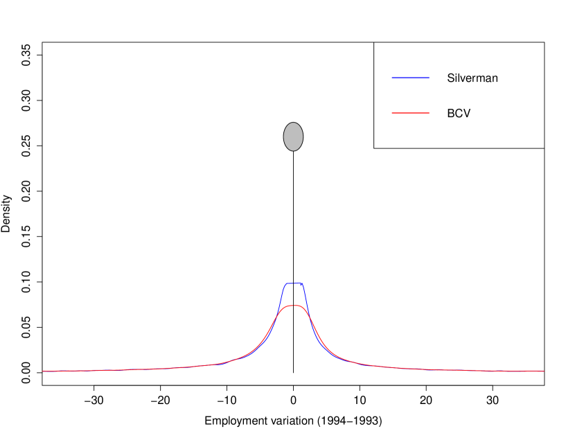
Figure 2: The estimated distribution of $Y_{it}^{D_{i}}-Y_{it_{0}}$ for $t=1994$ and $t_{0}=1993$. The probability of observing no variation is estimated by the proportion of observations such that $Y_{it}^{D_{i}}-Y_{it_{0}}=0$ whereas the continuous density of $Y_{it}^{D_{i}}-Y_{it_{0}}\neq 0$ is estimated thanks to kernel density estimators, with two different standard ways of selecting the bandwidth value. Silverman: Silverman’s rule of thumb; BCV: Biased Cross Validation (see Silverman, 1986; Sheather, 2004).

A relevant feature of this study is that the statistical units are generally demographically small and we observe no variation at all of the dependent variable along time for a non negligible fraction of the municipalities, i.e. $Y_{it}^{D_{i}}=Y_{it_{0}}$. Table A3 in the Supplementary file shows that the modal value of $Y_{it}^{D_{i}}-Y_{it_{0}}$ is indeed $0$ for all the values of $t$, with $t$ varying between 1994 to 2002 and $t_{0}$ corresponding to the year 1993. We can also remark that the fraction of zeros decreases with $t$ and varies with the treatment status. The estimated distribution of the dependent variable, $Y_{it}^{D_{i}}-Y_{it_{0}}$, for $t=1994$, which is a mixture of a mass at 0 and a continuous density function, is depicted in Figure 2.

Figure 2 about here

This empirical fact leads us to introduce a new econometric model that is able to take account of this important feature of the data. There is a kind of zero inflated effect that can not be dealt with a classical continuous response model. We thus allow $Y_{it}^{D_{i}}-Y_{it_{0}}^{0}$ to be equal to zero with a probability that may be strictly larger than $0$. Let us denote by $\Delta_{it}^{D_{i}}=\sum_{r=0}^{R-1}{\mathbbm{1}}_{\{D_{i}=r\}}\Delta_{it}^{r}$, with $\Delta_{it}^{r}=Y_{it}^{r}-Y_{it_{0}}^{0}$. We propose to describe the distribution of the counterfactual variation of the level of employment $\Delta_{it}^{r}$ as a mixture of a mass at $0$ and a continuous distribution. Using the decomposition $Y_{it}^{r}-Y_{it}^{0}=Y_{it}^{r}-Y_{it_{0}}^{0}-\left(Y_{it}^{0}-Y_{it_{0}}^{0}\right)$, we obtain that the expected conditional effect at time $t$ of policy $r$ compared to no policy is expressed as follows,

$$\mathbb{E}\left[Y_{it}^{r}-Y_{it}^{0}\mid X_{i}\right] =\mathbb{E}\left[Y_{it}^{r}-Y_{it_{0}}^{0}\mid X_{i}\right]-\mathbb{E}\left[Y_{it}^{0}-Y_{it_{0}}^{0}\mid X_{i}\right]$$

$$=\mathbb{E}\left[Y_{it}^{r}-Y_{it_{0}}^{0}\mid X_{i},\Delta_{it}^{r}\neq 0\right]\times\left(1-\mathbb{P}\left[\Delta_{it}^{r}=0\mid X_{i}\right]\right)$$ (4)

$$\ \ \ -\mathbb{E}\left[Y_{it}^{0}-Y_{it_{0}}^{0}\mid X_{i},\Delta_{it}^{0}\neq 0\right]\times\left(1-\mathbb{P}\left[\Delta_{it}^{0}=0\mid X_{i}\right]\right)$$ (5)

Expressions (4) and (5), which explicitly take account of the zero inflation feature of the counterfactual outcome variations, are the main object of interest in this paper.

3.3 A flexible semi-parametric modeling approach

Suppose now we have a sample $(Y_{it}^{D_{i}},X_{i},D_{i})_{i=1,\ldots,n}$, for $t\in\{t_{0},\ldots,t_{m}\}$. We can write

$$Y_{it}^{D_{i}}=\sum_{r=0}^{R-1}Y_{it}^{r}{\mathbbm{1}}_{\{D_{i}=r\}}$$ (6)

where the indicator function satisfies ${\mathbbm{1}}_{\{D_{i}=r\}}=1$ if $D_{i}=r$ and zero else. Consequently, we can express the expected variation along time $Y_{it}^{D_{i}}-Y_{it_{0}}^{0}$, of the employment level of municipality $i$ given that $\Delta_{it}^{D_{i}}\neq 0$, as follows,

$$\mathbb{E}\left[Y_{it}^{D_{i}}-Y_{it_{0}}^{0}|X_{i},\Delta_{it}^{D_{i}}\neq 0\right] =\mu_{t}^{0}(X_{i})+\sum_{r=1}^{R-1}{\mathbbm{1}}_{\{D_{i}=r\}}\alpha_{t}^{r}(X_{i}),$$ (7)

The term $\alpha_{t}^{r}(X_{i})$ which reflects in (7) the impact of treatment $r$ should be equal to zero when $t_{0}\leq t<t_{k}$ whereas $\mu_{t}^{0}(X_{i})$ corresponds to the expected variation under no policy.

Introducing (7) in (4) and (5), we can also express, given $X_{i}$, the expected effect of policy $r$ at time $t$ as follows

$$\mathbb{E}\left[Y_{it}^{r}-Y_{it}^{0}\mid X_{i}\right] =\left(1-\mathbb{P}\left[\Delta_{it}^{r}=0\mid X_{i}\right]\right)\times\alpha_{t}^{r}(X_{i})$$

$$-\left(\mathbb{P}\left[\Delta_{it}^{r}=0\mid X_{i}\right]-\mathbb{P}\left[\Delta_{it}^{0}=0\mid X_{i}\right]\right)\times\mu_{t}^{0}(X_{i}).$$ (8)

The conditional expected counterfactual in (8) is composed of two main terms that may act in opposite directions, so that interpretation is more difficult compared to usual policy evaluation models based on continuous response regression models that do not take account of the zero inflation effect.

In the econometric literature, a common practice consists in modeling $\mu_{t}^{0}(X_{i})$ and $\alpha_{t}^{r}(X_{i})$ using parametric specifications, where the $\mu_{t}^{0}(X_{i})$ is usually a linear function, $\mu_{t}^{0}(X_{i})=\mu_{t}^{0}+\sum_{j=1}^{p}\beta_{jt}^{0}X_{ij}$, and the term $\alpha_{t}^{r}(X_{i})$ does vary with the covariates or is expanded as a linear function of them (see e.g. Heckman and Hotz,, 1989, eq. 3.9). The linearity assumption is strong and a miss-specification of the relation between $Y_{it}^{r}-Y_{it_{0}}$ and the regressors may lead to wrong results and interpretation of the policy effect. We thus prefer to consider a more general model that can take account of non linear effects nonparametrically via an additive form (Hastie and Tibshirani, 1990; Wood, 2017). This also makes the underlying identification conditions less restrictive (Lechner, 2011a).

The expected value that would be obtained at time $t$ for a municipality with characteristics $X_{i}$ under no treatment, is supposed to be additively modeled as follows,

$$\mu_{t}^{0}(X_{i})=\mu_{t}^{0}+\sum_{j=1}^{p}g_{jt}^{0}(X_{ij}),$$ (9)

where $g_{jt}^{0}(.),\ j=1,\ldots,p$, are unknown smooth univariate functions. The identifiability constraints

$$\mathbb{E}\left[g_{jt}^{0}(X_{j})\ |\ \Delta_{t}^{0}\neq 0\right]=0,\quad j=1,\ldots,p,$$

ensure that $\mu_{t}^{0}$ represents the mean value of the variation of the potential outcome between $t$ and $t_{0}$ if all the units in the population would have received no incentives at all.

A key assumption of this paper is that the conditional differential policy effect $\alpha_{it}^{r}=\alpha_{t}^{r}(X_{i})$ can be expressed, given the vector of covariates $X_{i}$, with the following additive model,

$$\alpha_{it}^{r} =\alpha_{t}^{r}+\sum_{j=1}^{p}g_{jt}^{r}(X_{ij}),$$ (10)

where $g_{jt}^{r}(.),\ j=1,\ldots,p$ are unknown smooth functions satisfying the identifiability constraints

$$\mathbb{E}\left[g_{jt}^{r}(X_{j})|\ \Delta_{t}^{r}\neq 0\right]=0,\quad j=1,\ldots,p.$$

Consequently, $\alpha_{t}^{r}$ represents the mean effect, over the whole population, at period $t$ of treatment $r$ and the function $g_{jt}^{r}(.)$ reveals how the mean impact of the policy $r$ is modulated by the individual characteristics of each considered statistical unit.

Note that a simple extension of (10) consists in considering interactions between covariates instead of additive effects. For $2\leq d\leq p$, the additive effects of $d$ covariates, $g_{1t}^{r}(X_{i1})+g_{2t}^{r}(X_{i2})+\cdots+g_{dt}(X_{id})$ can be replaced by a more general multivariate function

$$\alpha_{it}^{r} =\alpha_{t}^{r}+g_{1,2,\ldots,d,t}^{r}(X_{i1},X_{i2},\ldots,X_{id})$$

that could allow a more flexible fit to the data, at the expense of a more difficult interpretability and, because of the curse of dimensionality, less precise estimates. The behavior of functions $g_{jt}^{r}$ is of central interest and our general model encompasses the following particular cases, i) no effect of the policy $r$ compared to no treatment at all, when $\alpha_{t}^{r}=0$ and $g_{jt}^{r}=0$ for all $t\geq t_{k}$; ii) linear trends in time when $\alpha_{t}^{r}=\alpha_{0}^{r}+\alpha_{1}^{r}t$ and linear effects of the covariates when $g_{jt}^{r}(X_{ij})=\beta_{jt}^{r}X_{ij}$ and iii) polynomial trends in time and polynomial effects of the covariates, as well as smooth threshold effects.

We suppose that the probability that $Y_{it}^{D_{i}}-Y_{it_{0}}=0$ given the covariates can be expressed with a generalized additive model and a logit link function. Using a similar decomposition as in (6), we consider the following logistic regression models, for $t=t_{1},\ldots,t_{m}$,

$$\mbox{logit}\left(\mathbb{P}\left[Y_{it}^{D_{i}}-Y_{it_{0}}^{0}=0\mid X_{i}\right]\right)=\beta_{0t}^{0}+\sum_{r=1}^{R-1}{\mathbbm{1}}_{\{D_{i}=r\}}\delta\beta_{0t}^{r}+\sum_{j=1}^{p}\beta_{jt}(X_{ij}),$$ (11)

where $\beta_{jt}(.)$ are unknown smooth univariate functions. For our purpose, the most important parameters are the differential effects $\delta\beta_{0t}^{r}$, $r=1,\ldots,R-1$. For example, if $\delta\beta_{0t}^{r}>0$, then the probability no variation is larger under policy $r$ compared to no policy at all ($r=0$) given the covariates $X_{i}=(X_{i1},\ldots,X_{ip})$. Recall that the unknown functions $\beta_{jt}(X_{ij})$ are not necessarily linear and that it would be possible to consider a more sophisticated model that could take interaction effects into account, replacing $\beta_{jt}(X_{ij})$ by $\beta_{jt}^{r}(X_{ij})$, for $r=1,\ldots,R-1$.

3.4 Estimation procedure

We observe, for a statistical unit $i$, the realized outcomes $Y_{it}^{{D}_{i}}$ at instants $t=t_{0},\ldots,t_{m}$, whereas the counterfactuals $Y_{it}^{r}$, for $r\neq D_{i}$, cannot be observed. The estimation of the parameters and functions defined in (9), (10) and (11), relies on the sample $(Y_{it}^{D_{i}},X_{i},D_{i})_{i=1,\ldots,n}$, for $t\in\{t_{0},\ldots,t_{m}\}$. We assume that there are no spatial interactions between the statistical units so that $(Y_{it}^{D_{i}},X_{i},D_{i})$ and $(Y_{\ell t}^{D_{\ell}},X_{\ell},D_{\ell})$ can be supposed to be independent if $i\neq\ell$. This hypothesis can be easily relaxed by allowing, for instance, spatial spillover effects via the definition of additional covariates that take account of the treatments received by the neighboring municipalities (see Appendix C). The $t_{m}-t_{0}$ samples $(Y_{it}^{D_{i}}-Y_{it_{0}}^{0},X_{i},D_{i})_{i=1,\ldots,n}$, with $t=t_{1},\ldots,t_{m}$ are used separately to estimate the parameters of interest and the regression functions.

The fact that the considered mixture is a mixture of a continuous variable and a discrete variable makes the computation of the likelihood rather simple compared to mixtures of continuous variables or mixtures of discrete variables (see McLachlan and Peel (2000)). Indeed, as far as the continuous part is concerned, the probability of no variation is equal to zero and we can proceed as if the two underlying distributions were adjusted separately. Assuming $(Y_{it}^{D_{i}}-Y_{it_{0}}^{0},\ i=1\ldots,n)$ are conditionally Gaussian and independent random variables, the likelihood at each instant $t$, is given by

$$\mathcal{L}_{t}=\prod_{i=1}^{n}p_{it}^{T_{it}}(1-p_{it})^{1-T_{it}}f_{t}^{D_{i}}(Y_{it}^{D_{i}}-Y_{it_{0}}^{0};X_{i},D_{i})^{1-T_{it}}$$

where $T_{it}={\mathbbm{1}}_{\{\Delta_{it}^{D_{i}}=0\}}$ is the indicator function of no variation between $t$ and $t_{0}$ and $p_{it}=\mathbb{P}\left[\Delta_{it}^{D_{i}}=0\mid X_{i},D_{i}\right]$. Taking account now of the different policies, the log-likelihood can be expressed as follows,

$$\ln\mathcal{L}_{t} =\sum_{i:T_{it}=1}\ln p_{it}+\sum_{i:T_{it}=0}\ln(1-p_{it})$$ (12)

$$+\sum_{i:T_{it}=0}\sum_{r=0}^{R-1}{\mathbbm{1}}_{\{D_{i}=r\}}\ln f_{t}^{r}(Y_{it}^{D_{i}}-Y_{it_{0}}^{0};X_{i},D_{i}),$$ (13)

so that the probability of no variation can be estimated separately by maximizing the terms at the right-hand side of (12), whereas the additive models related to the continuous variation of $Y_{t}^{D}-Y_{t_{0}}^{0}$ are estimated by maximizing the function at the right-hand side of (13). This means that in practice, the subsample $\{i\ |T_{it}=0\}$ is used for the adjustment of the additive models related to the continuous part. The estimation of the unknown functional parameters introduced in (9), (10) and (11), which are supposed to be smooth functions, is performed thanks to the mgcv library in the R language (see Wood, 2017, for a general presentation). The regression functions to be estimated are expanded in spline basis and a penalized likelihood criterion is maximized. Penalties, tuned by smoothing parameters, are added to the log-likelihood in order to control the trade off between smoothness of the estimated functions and fidelity to the data. To select the values of the smoothing parameters, restricted maximum likelihood (REML) estimation was preferred over alternative approaches such as Generalized Cross Validation (GCV) or Akaike’s Information Criterion (AIC), since such approaches may lead to under-smoothing and are more likely to develop multiple minima than REML. Pointwise confidence intervals that take account of the smoothing parameter uncertainty can be obtained as in Wood et al., (2016) and variable selection is performed following Marra and Wood (2011).

4 Results

The main goal of this paper is the estimation of the mean differential effect, $\mathbb{E}\left[Y_{it}^{r}-Y_{it}^{0}\mid X_{i}\right]$, of policy $r$ compared to no policy, for a unit with characteristics $X_{i}$. This conditional expectation, which is expressed in (8), depends on different ingredients. Estimations of $\alpha_{t}^{r}(.)$ and $\mu_{t}^{0}(.)$ are related to the continuous part of the model while the discrete one provides us information about the conditional probabilities $\mathbb{P}\left[\Delta_{it}^{r}=0\mid X_{i}\right]$ and $\mathbb{P}\left[\Delta_{it}^{0}=0\mid X_{i}\right]$.

After a discussion about the parameters of interest, we briefly present some preliminary estimation results for both the continuous and the discrete part of the model, taken separately. We then provide our main results. Since our model allows the policy effect to vary both in time and across units, we specifically provide a temporal counterfactual analysis at an individual level, with an illustration on a few representative municipalities for which the evolutions of the potential outcomes are estimated and compared under the different possible treatments. This could provide interesting economic and policy oriented advices. We finally provide some insights into the size of bias that may arise when a parametric specification is imposed or the mass of observations at zero is not not accounted for, by comparing the proposed approach with some standard methods.

4.1 Parameters of interest

We focus on the assessment of ZRR and 5B as well as their joint mean effect. The partial overlap of these two schemes makes possible the identification of the interaction effect of ZRR and 5B. We thus adopt a framework with $R=4$ multiple potential outcomes and consider the generalized treatment variable, D${}_{i}\in\left\{0,ZRR,5B,ZRR\&5B\right\}$ indicating the programme in which municipality $i$ actually participated. The modality $0$ indicates that the municipality i did not receive any policy, $ZRR$ (respectively $5B$) indicates that the municipality i received incentives only from ZRR (respectively only from 5B) and $ZRR\&5B$ indicates that the municipality i received incentives both from ZRR and 5B.

As far as the continuous response is concerned, the parameter $\alpha_{t}^{5B}$ measures the mean differential effect, over the whole sample, of policy 5B compared to no policy at all ($r=0$) whereas the joint effect of ZRR and 5B is given by $\alpha_{t}^{ZRR\&5B}$. Finally, concerning the effect of ZRR, it can be noticed that only a few municipalities (precisely 722) are treated in this case. Consequently, we prefer to focus our attention on the 7014 municipalities that receive incentives both from 5B and ZRR and we calculate the following differential effect $\alpha_{t}^{ZRR}=\alpha_{t}^{ZRR\&5B}-\alpha_{t}^{5B}$. This differential effect simply represents the mean difference between the outcome when receiving incentives both from ZRR and 5B and the outcome when only 5B applies. The same reasoning applies to the interpretation of the expected conditional differential effect $\alpha_{it}^{r}$ in (10) as well as for the parameter $\delta\beta_{0t}^{r}$ when dealing with the estimation of the conditional probability of a null employment variation in (11).

4.2 Preliminary results

The continuous response

As far as the continuous response is considered, additive models are fitted on the subsamples $\{i\ |Y_{it}^{D_{i}}-Y_{it_{0}}\neq 0\}$. We focus attention on the expected conditional differential effect $\alpha_{it}^{r}$, for $t_{k}\leq t\leq t_{m}$ and $r\in\{1,\ldots,R-1\}$, while the results about the effect of the initial conditions, which enter nonparametrically via the additive smooth functions $\sum_{j=1}^{p}g_{jt}^{0}(X_{ij})$ in (9), are not discussed here but are available upon request.

A backward variable selection procedure has been employed to select the variables to be introduced in the regression functions defined in (9) such that the conditional independence assumption (3) holds. This procedure leaded us to retain 11 variables among the 16 initial variables (the selected variables are those reported in Table A2 in the Supplementary file).

We consider pre-treatment covariates, say $X_{pre},$ in the set of observable variables $X$ to ensure that $D$ causes $X$ and $Y$ causes $X$ do not occur. This is likely to be relevant in our economic context where it could be expected that the covariates prior the introduction of the policy, such as for example the share of qualified workers or the existing stock of infrastructure, cause both the inclusion in the program $D$, and the potential local employment $Y$ ($X_{pre}\rightarrow D$ and $X_{pre}\rightarrow Y)$. After the introduction of the policy, the level of such covariates, say $X_{post}$, is likely to be affected by its past values $X_{pre}$, by the treatment $D$ and finally also by the response variable $Y$. Indeed, in the example mentioned above, the share of qualified workers and the stock of infrastructure may be directly affected by the policy ($D\rightarrow X_{post}$) and since the introduction of the policy could have also increased local employment ($D\rightarrow Y$), this may in turn stimulate the creation of new infrastructure/qualified hires ($Y\rightarrow X_{post}$). In such a causal framework, $X_{pre}$ should be controlled for whereas $X_{post}$ should not (see Lee,, 2005; Lechner, 2011a).

Also note that the vector $X_{i}$ may contain the initial level of employment. Including the initial outcome as a regressor is particularly relevant if the average outcomes of the treated and the control groups differ substantially at the first period, as in this case (see e.g. Imbens and Wooldridge, 2009; Lechner, 2015)

As expected, the initial outcome was found highly significant and has been included. In almost all cases the linearity was clearly rejected in favor of nonlinear regression functions. We  also remark that not imposing a linear relation in (9) leads to retain a larger number of significant variables compared to simpler linear regression models since there are only 6 significant variables when imposing linear relations.

Since a major interest lies in assessing possible heterogeneous treatment effects, we examine how the effect of a policy may vary with some economic or demographic characteristics of the municipalities. For that purpose, we consider a generalization of model (10) in which interactions between variables are allowed. The model selection procedure allowed us to retain only two significant variablesto fit $\alpha_{it}^{r},$ in (10): the initial level of employment (SIZE) of the municipality and its population density (DENSITY). Using an approximate ANOVA test procedure (see Wood, 2017), an additive structure for $\alpha_{it}^{r}$, i.e $\alpha_{it}^{r}=\alpha_{t}^{r}+$ $g_{1t}^{r}(\mbox{{SIZE}}_{i})+g_{2t}^{r}(\mbox{{DENSITY}}_{i})$ is strongly rejected for all years $t$ in favor of a more general model based on bivariate regression functions,

$$\alpha_{it}^{r}=\alpha_{t}^{r}+g_{t}^{r}(\mbox{{SIZE}}_{i},\mbox{{DENSITY}}_{i}),\quad r=1,\ldots,R-1.$$

As seen in Table A5 in the Supplementary file, a first result that emerges is that the estimates of the parametric part of (10), representing the mean effect of the policies for the subsamples $\{i\ |Y_{it}^{D_{i}}-Y_{it_{0}}\neq 0\},$ i.e. $\alpha_{t}^{r},$ indicate a very short-run (abrupt but transitory) and quite low mean effect of ZRR. Indeed, the estimated value of $\alpha_{t}^{ZRR}$ for the pre-program years is close to zero and is clearly not significant; then, it grows and rises up to $2.159$ (p-values$=0.063$)  when $t=1999$. Afterwards, it sharply decreases and becomes close to zero again at the end of the period. It is instead highlighted a gradual start, long-term duration mean effect for the joint 5B-ZRR treatment since $\widehat{\alpha}_{t}^{5ZRR\&5B}$ grows overtime, reaching the pick of $3.537$ (p-values$=0.001$)  when $t=1999$ and then it slowly decreases over time. Finally, $\widehat{\alpha}_{it}^{5B}$ has a similar time pattern than $\widehat{\alpha}_{t}^{ZRR\&5B}$ but it is not significant at standard levels.

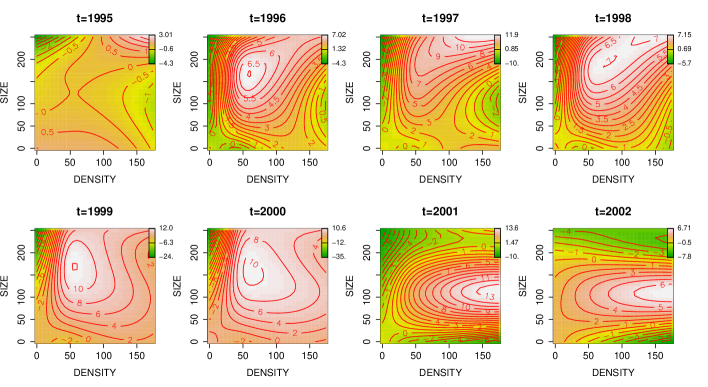
(b) ZRR&5B

(c) 5B

Figure 3: Contour plots of $\widehat{g}_{t}^{r}(\mathtt{SIZE},\mathtt{DENSITY}).$

Next, the examination of the nonparametric part $g_{t}^{r}\left(.\right)$ of (10), reveals how the mean impact of the policy $r$ varies as a function of the characteristics in terms of density and size of each considered statistical unit (see Figure 3).

Figure 3 about here

In almost all cases, the smooth functions appear to be highly significant, using a Bayesian approach to variance estimation (Wood, 2012), with generally quite high effective degrees of freedom, thus indicating rather complex functions (see Wood, 2017). For all the treatments, we first note that both the magnitude and the shape of the nonparametric effect vary with time. Looking at ZRR, the estimated smooth function $\widehat{g}_{t}^{ZRR}(\mathtt{SIZE}_{i}\mathtt{,DENSITY}_{i})$ is very flat and close to zero at the beginning and at the end of the period whereas it becomes clearly nonlinear with a bell-shaped pattern for a period of a few years after the introduction of the policy. The maximum of these functions is generally reached for levels of DENSITY slightly above 50 and for levels of SIZE at about 150, even if the location of these maxima slightly change over time. For the last two years, the maximum is reached for slightly smaller and denser municipalities. Note that in the plots, the domain of SIZE and DENSITY has been appropriately reduced to focus on municipalities not having a too large sizes or very high levels of density. The joint nonparametric effect of ZRR and 5B, $\widehat{g}_{t}^{ZRR\&5B}(\mathtt{SIZE}_{i}\mathtt{,DENSITY}_{i})$ behaves similarly in terms of shape and time pattern but with a stronger effect for the years 1999 and 2000. Finally, the estimated nonparametric surface measuring the effect of 5B, $\widehat{g}_{t}^{5B}(\mathtt{SIZE}_{i}\mathtt{,DENSITY}_{i})$, is generally quite flat, even if some positive effects appeared for rather low levels of DENSITY and for $t\geq 1999.$

Modeling the probability of no variation

Generalized additive models based on binomial regression with logit link function are fitted to estimate the probability that a variation of the response between $t$ and $t_{0}$ does not occur, given the treatment status and the initial conditions. This conditional probability is expressed in (11).

Again, a backward variable selection procedure has been employed to select the variables to be introduced in the model. The estimation results are presented in Table A5 and indicate that the 5B program has a negative effect on the probability that employment does not vary along time. The estimated parameter $\widehat{\delta\beta}_{0t}^{5B}$ is always negative, in a significant way for nearly all instants $t$. Referring to (11), this means that $\mathbb{P}\left[\Delta_{it}^{5B}=0\mid X_{i}\right]-\mathbb{P}\left[\Delta_{it}^{0}=0\mid X_{i}\right]<0$.  When, looking at ZRR, it can be noted that the estimated parameter $\widehat{\delta\beta}_{0t}^{ZRR}$ is always positive, but is not significant in most of the cases, so that $\mathbb{P}\left[\Delta_{it}^{ZRR}=0\mid X_{i}\right]-\mathbb{P}\left[\Delta_{it}^{0}=0\mid X_{i}\right]$ is not significantly different from zero. Finally, the estimated joint policy effect $\widehat{\delta\beta}_{0t}^{ZRR\&5B}$ is always very close to zero and is never significant.

As far as the mean differential effect, $\mathbb{E}\left[Y_{it}^{r}-Y_{it}^{0}\mid X_{i}\right]$ in (8) is concerned, these results suggest that, for both ZRR and the joint policy ZRR&5B, this differential effect is mostly affected by the first part of the expression, i.e. by $\left(1-\mathbb{\ P}\left[\Delta_{it}^{r}=0\mid X_{i}\right]\right)\times\alpha_{t}^{r}(X_{i})$. Conversely, for 5B, there is an additional effect arising from the second part of the expression, since, as noted before, $\mathbb{P}\left[\Delta_{it}^{5B}=0\mid X_{i}\right]-\mathbb{P}\left[\Delta_{it}^{0}=0\mid X_{i}\right]<0$.

4.3 Main results

Counterfactual analysis at an individual level

We now provide the main results of the estimation and combine information from the two parts, the continuous and the discrete one, of the mixture model. Notably, our nonparametric approach allows for non-linear and local effects and thus make it possible to conduct a temporal counterfactual analysis at an individual level. This relevant feature is illustrated on a few representative municipalities for which the evolutions of the potential outcomes are estimated and compared under the different possible treatments. These municipalities have been chosen with a clustering partition around medoids procedure (see Kaufman and Rousseeuw, 1990) with four clusters so that they represent four different homogeneous groups. Descriptive statistics are given in Table 1.

Table 1 about here

Using (4), (5), (10) and (11) we can estimate what would have been the evolution of the expected effect of each municipality under each policy, taking account of the zero inflation effect. We are also interested in building confidence intervals. Due to the complexity of our statistical estimations at an individual level, which are products of predictions obtained with generalized additive models, the standard delta method cannot be used easily. We consider instead the more flexible bootstrap approach (see e.g. Efron and Tibshirani, 1993) to approximate the distribution of the conditional counterfactual outcome of each selected municipality $i$ having characteristics $X_{i}$.

We draw $B=1000$ bootstrap samples and for each bootstrap sample $b$, with $b=1,\ldots B$, we make the following estimation of the expected counterfactual evolution (see (8)),

$$\widehat{\mathbb{E}}^{b}\left[Y_{it}^{r}-Y_{it}^{0}\mid X_{i}\right] =\left(1-\widehat{\mathbb{P}}^{b}\left[\Delta_{it}^{r}=0\mid X_{i}\right]\right)\times\widehat{\alpha}_{t}^{r,b}(X_{i})$$

$$-\left(\widehat{\mathbb{P}}^{b}\left[\Delta_{it}^{r}=0\mid X_{i}\right]-\widehat{\mathbb{P}}^{b}\left[\Delta_{it}^{0}=0\mid X_{i}\right]\right)\times\widehat{\mu}_{t}^{0,b}(X_{i}),$$

where $\widehat{\mathbb{P}}^{b}\left[\Delta_{it}^{r}=0\mid X_{i}\right]$ is the estimated probability, with sample $b$, of no employment variation and $\widehat{\alpha}_{t}^{r,b}(X_{i})$ and $\widehat{\mu}_{t}^{0,b}(X_{i})$ are the fitted values. Then, we can deduce, using the percentile method, bootstrap confidence intervals for the conditional expectation $\mathbb{E}\left[Y_{it}^{r}-Y_{it}^{0}\mid X_{i}\right]$, i.e the mean effect at time $t$ on municipality with characteristics $X_{i}$ of treatment $r$ compared to no treatment.

Temporal policy effects for the selected municipalities

Estimated expected counterfactual values as well as bootstrap confidence intervals are drawn in Figure 4 for the four municipalities under study. The first selected municipality, which is named DSI1, is an extremely dense and urbanized municipality, with values of DENSITY and URB greater than the 95th percentile. It is also very rich in terms of INCOME and big in terms of SIZE, with values of these variables about the 80th percentile. For this municipality, we estimate a positive evolution of employment in the absence of any policy. We can also note that, according to our model, ZRR, 5B and the joint policies ZRR&5B would have no significant effect on the evolution of employment for the considered period. .

The second municipality, named DS3, is rather dense, urbanized and big, with values of DENSITY, URB and SIZE about the 75th percentile of our sample. The value of INCOME is close to the median. We note that the effect of 5B is quite low – and is only significant for $t=1997$ and $t=1998$ – and presents a rather flat evolution over time, whereas both ZRR and the joint policy ZRR&5B have a higher impact on employmememt, with an inverted U pattern. Such an impact increases over the years reaching a peak for $t=1999$ and then it slowly decreases during the following years.

Figure 4 about here

The third municipality, DSI3, is quite close to the median values in terms of DENSITY and SIZE. For this municipality, all the policies produce an effect with an inverted U time pattern, even if the effect of ZRR is significant only for a short period, i.e. over 1998-2001. Finally, for the last municipality DSI7, which is a small and poor municipality, there is a clear positive effect of 5B over all the period (except the last year), with again an inverted U pattern over time. For this municipality, ZRR has instead no significant effect over the whole period.

These results highlight that ZRR and 5B are likely to produce temporal effects that vary according to the typology of the municipalities. Indeed, while the structural funds 5B are effective for very small and rural municipalities, the fiscal incentives through ZRR produce an effect for bigger and more dense/urbanized areas. This result is consistent with the idea that agglomeration externalities (Devereux et al., 2007) and an adequate size of the local market are essential in order to make such fiscal incentives effective, while the structural funds, which mainly cover investments in infrastructure, technology and productive assets, may produce an effect even for very deprived areas. Finally, the lack of effects for extremely dense and big municipalities is not surprising because only few municipalities with such characteristics are treated and the policies under investigation have not been designed for such a typology of municipality.

Our results can be seen as a refinement of previous studies focusing on average effects. As far as the French experience is concerned, Behaghel et al., (2015) did not find any significant average effect of ZRR at a canton level over the period, even if they underlyine that “this lack of effect may hide positive impacts on some specific segments” (Behaghel et al.,, 2015, p. 9). It can be also noted that beyond the French experience, the literature generally provides mixed evidence. In some papers a significant effect on employment (Papke, 1994; Ham et al., 2011) is noted for such policies whereas some other works indicate that EZ have been ineffective (Bondonio and Engberg, 2000; Neumark and Kolko, 2010), or only provide a transitory effect  (O’Keefe, 2004). Moreover, as far as the structural funds are concerned, Becker et al., (2010) focus attention on the effect of Objective 1 on regional growth for NUTS2 and NUTS3 regions and find evidence of temporal effects, with an average effect that takes four years to become significant and increases afterwards up to the sixth and last available year after its introduction. Overall, we provide evidence that allowing the effect of the policy to vary in time and across municpalities can be useful to show the existence of temporal effects over short periods of time for some specific municipalities, which otherwise could be missed when looking at average effects over time. The next subsection will provide further insights on such an issue.

A comparison with standard parametric approaches

As a final step, we compare the proposed approach with some standard methods, which are based on parametric models or which do not account for the mass at zero. This may provide relevant insights because, as stressed for instance by Lechner (2011a), the size of the bias of misspecified parametric models can be assessed only through a comparison. The models we consider are listed below:

• Model 1: Linear continuous response model with homogeneous temporal effect, $\mu_{t}^{0}(X_{i})=\mu_{t}^{0}+\sum_{j=1}^{p}\beta_{jt}^{0}X_{ij};$ $\alpha_{it}^{r}=\alpha_{t}^{r}.$

• Model 2: Linear continuous response model with linear policy interactions, $\mu_{t}^{0}(X_{i})=\mu_{t}^{0}+\sum_{j=1}^{p}\beta_{jt}^{0}X_{ij};$ $\alpha_{it}^{r}=\alpha_{t}^{r}+\gamma_{t}^{r}\mathtt{SIZE}_{i}+\theta_{t}^{r}\mathtt{DENSITY}_{i}.$

• Model 3: Linear mixture distribution model with linear policy interactions, $\mu_{t}^{0}(X_{i})=\mu_{t}^{0}+\sum_{j=1}^{p}\beta_{jt}^{0}X_{ij};$ $\alpha_{it}^{r}=\alpha_{t}^{r}+\gamma_{t}^{r}\mathtt{SIZE}_{i}+\theta_{t}^{r}\mathtt{DENSITY}_{i}$.

• Model 4: Additive mixture distribution model with nonparametric policy interactions, $\mu_{t}^{0}(X_{i})=\mu_{t}^{0}+\sum_{j=1}^{p}g_{jt}^{0}(X_{ij});$ $\alpha_{it}^{r}=\alpha_{t}^{r}+g_{t}^{r}(\mathtt{SIZE}_{i},\mathtt{DENSITY}_{i})$.

The first model is a continuous parametric response model. It is simple extension of the difference-in-differences estimator that allows for temporal policy effects and that takes account of linear effects of the initial conditions. This model is very standard in the policy evaluation literature. Also, note that in Model 1,  the policy effect does not change across municipalities. The second one allows the term $\alpha_{it}^{r}$ to be a linear function of SIZE and DENSITY. The third one extends the previous one by handling the zero inflation effect. Finally, the fourth model is the one we propose in this paper allowing for additive smooth effects of the initial conditions, nonparametric policy interactions and handling the zero inflation phenomenon.

Figure 5 about here

As an illustrative example, we focus on municipality DSI3, whose values of SIZE and DENSITY are close to the median. The results are depicted in Figure 5. As far as Model 1 is concerned, we note that none of the policies is found to provide a significant effect, the only exception being the joint 5B-ZRR policy at time $t=1999$. This result appears to be in sharp contrast with the results from the proposed Model 4, which highlights nonlinear and significant temporal effects for all the treatments. We can also remark the big difference concerning the estimated employment under no treatment when comparing the two approaches. Then, when moving to Model 2/Model 3, some temporal effects appear, even if, by imposing a parametric policy interaction, $\alpha_{it}^{r}=\alpha_{t}^{r}+\gamma_{t}^{r}\mathtt{SIZE}_{i}+\theta_{t}^{r}\mathtt{DENSITY}_{i}$, we obtain very different time patterns of the estimated effects compared to the ones obtained with the more flexible Model 4. Specifically, while models 2 and 3 indicate a monotonically increasing overtime effect of 5B and an increasing effect of ZRR, with a threshold for the last years in the sample, Model 4 suggests an inverted U pattern for both policies. Finally, it is worth comparing Model 2 with Model 3, where the only difference is the fact of accounting or not for the mass of observations at zero. When comparing these two models, it can be noted that the policy effects present similar temporal patterns but handling the zero inflation feature of the data makes increase the estimated policy effect of about 15% -20%. The same result is obtained when comparing Model 4 with a similar model that does not account for the mass of observations at zero.We finally note that allowing for nonlinear effects of the initial conditions greatly affects the estimates of the policy effects. As an example, when we estimate a model similar to model 4 by imposing the restriction $\alpha_{it}^{r}=\alpha_{t}^{r}$, we find evidence of significant temporal effects, while when we also impose linear effects of the initial conditions, we do not find any significant effect as in Model 1.

5 Concluding remarks

In this paper, we introduce a semi-parametric approach to estimate the variation along time and across municipalities of regional treatment effects in France. Since we face a kind of zero inflated phenomenon that cannot be dealt properly with a continuous distribution, we consider a mixture distribution model that combines a Dirac mass at zero and a continuous response. We rely on additive models for the continuous response and generalized additive models for modeling the probabiltiy of a mass at zero, giving more flexibility than linear models, and we exploit the longitudinal structure of the data to account for selection bias.

We find that the different policies under investigation are likely to produce temporal effects that vary according to the typology of the municipalities. We also documented that using the proposed semi-parametric model that allows the effect of the policy to vary in time and across municipalities is crucial to show the existence of temporal effects over short periods of time for some specific municipalities, which otherwise will be missed when using standard parametric approaches. We finally provide evidence that accounting for the mass of observation at zero is important to avoid a substantial underestimation of the effect of the policies.

This work provides new results about the pattern of temporal treatment effects and nonlinear interactions, as well as some guidance for future research. It first suggests, within a flexible semi-parametric regression framework, a way to deal with an excess of zeros by considering a mixture of a continuous and a discrete distribution. This may be relevant for other policy evaluations when the dependent variable does not vary along time for a non-negligible fraction of the units. Second, the consideration of a model in which the effect of the policy is expanded as a nonparametric function of the covariates provides a richer framework that allows for a finer analysis and permits to perform a counterfactual estimation at an individual level. This could be relevant in many cases in which heterogeneous policy effects are likely to be present or when there is an interest in units having some peculiar characteristics.

Finally note that the proposed model is flexible and modular enough so that it can be extended in various directions. In our opinion, an extremely relevant issue concerns the possible existence of policy effects on neighboring municipalities, i.e. spatial spillover effects (see e.g. Behaghel et al.,, 2015). Appendix C in the Supplementary material indicates that using our local approach, instead of focusing on average effects, can be crucial to highlight the existence of significant spillover effects and suggests that further studies may deepen such an issue.

		$D$	$\longrightarrow$	$Y_{t}^{r}-Y_{t_{0}}$
	$\mathbf{\nearrow}$	$\uparrow$	$\nearrow$	$\uparrow$
$X_{\bar{Y}\cap D}$		$X_{Y\cap D}$		$X_{Y\cap\bar{D}}$

Figure 1: The expected causal relation between $Y_{t}^{r}-Y_{t_{0}}$, $X$ and $D$

(a) ZRR

Supplementary Material

Appendix A Data, variables and sample

After the merge of the different sheets provided by the INSEE containing information on local employment, the demographic structure, education and land use, we get a data set containing 36000 municipalities, that is the 98,5% of the French municipalities. While the paper focuses specifically on rural development policies, it is worth recalling that a relevant fraction of the municipalities received structural funds (1994-99) not specifically devoted to rural development. These are the Objective 1 and the Objective 2 funds. Objective 1 has the explicit aim of fostering per capita GDP growth in regions that are lagging behind the EU average - defined as those areas with a per capita GDP of less than 75 per cent of the EU average - and of promoting aggregate growth in the EU. Objective 2 covers regions struggling with structural difficulties and aims to reduce the gap in socio-economic development by financing productive investment in infrastructures, local development initiatives and business activities. Table A1 describes the distribution of the municipalities according to the ZRR and the structural funds schemes (1994-99).

Among the 646 municipalities under Objective 1, 350 are located in Corsica. All the Corsica’s municipalities available in our dataset are under the Objective 1. Among them, 268 were also under ZRR scheme. The remaining 296 municipalities under Objective 1 are located in the region Nord-Pas de Calais and were not under ZRR. Given the small number of municipalities under the Objective 1 and their specific characteristics, we decided to remove them from the analysis. This simplifies greatly the framework of the analysis without losing a relevant amount of information, getting a dataset containing 35354 municipalities.

As far as Objective 2 is concerned, we initially estimated the proposed model by including a treatment variable defined as $D_{i}\in\left\{0,EU2,5B,ZRR,ZRR\&EU2,ZRR\&5B\right\}$, which also accounts for the Objective 2, $EU2$ ($ZRR\&EU2)$ indicating that the municipality i receive incentives only from Objective 2 (from both Objective 2 and ZRR). However, the estimated parameters $\widehat{\alpha}_{t}^{EU2}$  and $\widehat{\alpha}_{t}^{ZRR\&EU2}$ ($\widehat{\delta\beta}_{0t}^{EU2}$ and $\widehat{\delta\beta}_{0t}^{ZRR\&EU2}$) were always very close to zero and never significant with p-values very far from standard significance levels. This result along with the fact that the interest of this paper is on rural development, motivated the use of the treatment variable defined in Section IV where the Objective 2 municipalities are considered as if they had not received any treatment. The use of such a variable simplifies the analysis and the presentation of the results without losing relevant information, also provided that the four parameters of interest $\alpha_{t}^{5B},$ $\alpha_{t}^{ZRR\&5B}$ and $\alpha_{t}^{ZRR}$ ($\delta\beta_{0t}^{5B},$ $\delta\beta_{0t}^{ZRR\&5B}$ and $\delta\beta_{0t}^{ZRR}$) are fundamentally not affected by such a choice.

The dependent variable $Y_{it}$ ($i$ indicating the municipality; and $t$ the time $t=1993,...,2003$) measures the number of employees and has been calculated from the SIRENE data sheet covering manufacture, trade and services, while the initial full set of regressors (measured at time $t=1990$) is composed of the following 16 variables:

Initial outcome

$\mathtt{SIZE}_{i}\equiv Y_{it_{0}}$ is the initial outcome, i.e the level of employment at $t_{0},$ with $t_{0}$ equals to $1993$;

Socio-economic and demographic variables

$\mathtt{DENSITY}_{i}\equiv\left(\text{{population}}\right)_{i}/\left(\text{{surface in terms of \ km}}^{2}\right)_{i};$

$\mathtt{OLD}_{i}\equiv\left(\text{{population over 65}}\right)_{i}/\left(\text{{total population}}\right)_{i};$

$\mathtt{INC}_{i}\equiv\left(\text{{net taxable income}}\right)_{i}/\left(\text{{total population}}\right)_{i};$

$\mathtt{FACT}_{i}\equiv\left(\text{{number\ of} {factory\ workers}}\right)_{i}/\left(\text{{total\ population}}\right)_{i}$;

$\mathtt{EXE}_{i}\equiv\left(\text{{number\ of} {executive\ workers}}\right)_{i}/\left(\text{{total\ population}}\right)_{i}$;

$\mathtt{FARM}_{i}\equiv\left(\text{{number\ of} {\ farmers}}\right)_{i}/\left(\text{{total\ population}}\right)_{i}$;

$\mathtt{UNIV}_{i}$ $\equiv\frac{\left(\text{{number\ of\ people\ with\ a\ master\ level\ degree called \textquotedblleft Ma\^{\i}trise universitaire\textquotedblright}}\right)_{i}}{\left(\text{{total\ population}}\right)_{i}}\ \$;

$\mathtt{BTS}_{i}\equiv\frac{\left(\text{{number\ of\ people\ with\ a\ \ technical} {degree called\ \textquotedblleft Brevet de Technicien Sup\'{e}rieur\textquotedblright}}\right)_{i}}{\left(\text{{total\ population}}\right)_{i}}$;

$\mathtt{NOEDU}_{i}$ $\equiv\left(\text{{number\ of\ people\ without\ a} {degree}}\right)_{i}/\left(\text{{total\ population}}\right)_{i}$;

Land use

$\mathtt{AGRI}_{i}\equiv$ $\left(\text{{farmland} {surface}}\right)_{i}/\left(\text{{total\ surface}}\right)_{i}$;

$\mathtt{CULT}_{i}\equiv$ $\left(\text{{cultivated land} {surface}}\right)_{i}/\left(\text{{total\ surface}}\right)_{i}$;

$\mathtt{URB}_{i}\equiv$ $\left(\text{{urban surface}}\right)_{i}/\left(\text{{total\ surface}}\right)_{i}$;

$\mathtt{IND}_{i}\equiv$ $\left(\text{{industrial surface}}\right)_{i}/\left(\text{{total\ surface}}\right)_{i}$;

$\mathtt{ARA}_{i}\equiv$ $\left(\text{{arable surface}}\right)_{i}/\left(\text{{total\ surface}}\right)_{i}$;

$\mathtt{GRA}_{i}\equiv$ $\left(\text{{grassland surface}}\right)_{i}/\left(\text{{total\ surface}}\right)_{i}$;

The socio-economic and demographic variables come from standard INSEE sources while the variables measuring land use have been obtained from the “Corine Land Cover” base (providing remote sensing images which have been merged with the French map at a municipality level).

The retained models, those results are presented in Section 4, have been obtained using a backward selection procedure starting from the above set of potential explanatory variables. Backward selection provided almost the same results as the double penalty approach proposed by Marra and Wood (2011), those detailed results are available upon request.  More precisely, we selected the variables equation-by-equation for $t=1994,...,2002,$ by setting the threshold level for the p-values to $0.01$ and in the end, to use the same explanatory variables  for all $t$, we choosed the variables that were 1% significant at least for one time period, $t$. According to the notation used in Section 3, these variables are noted as $X_{Y\cap D}$ and $X_{Y\cap\bar{D}}.$

For the estimation of the conditional probability of a null employment variation along time which is expressed in eq. (11), we retained the following variables:

$$X_{i}^{\{\text{{logit}}\}}=\left(SIZE_{i},DENSITY_{i},UNIV,INC,FACT_{i},EXE,FARM,BTS_{i},NOEDU,ARA_{i},URB_{i},IND_{i},GRA\right),$$

while for the continuous part of the model referring to the subsample $\{i\ |Y_{it}^{D_{i}}-Y_{it_{0}}\neq 0\}$,  the variables that we selected are:

$$X_{i}^{\{\text{{continuous}}\}}=\left(SIZE_{i},DENSITY_{i},OLD_{i},INC,FACT_{i},BTS_{i},CULT_{i},AGRI_{i},ARA_{i},URB_{i},IND_{i}\right).$$

Tables A2 and A3 provide simple descriptive statistics.

Also note that according to Heckman and Hotz (1989, pg. 865), selection bias may also arise from the presence of variables that may influence selection into the program even if they do not affect directly the outcome and introducing these variables into the regression solves this additional source of selection bias. Using the notation employed in Section 3, these variables are noted as $X_{\bar{Y}\cap D}.$ We determine these variables by exploiting recent advances in generalized additive models permitting the estimation of multinomial logistic regression (Wood et al.,, 2016). This allows a flexible estimation of a generalized propensity score $\mathbb{P}\left[D_{i}\mid X_{i}\right]$ as a function of additive smooth components. Again we used the backward selection and finally we added 3 more variables that appeared to affect selection into the programs and that were not selected directly from the outcome equation. These variables are $FARM_{i}$, $NOEDU_{i}$ and $GRA_{i}.$  However, adding these variables does not produce relevant changes to the estimates of the effects and detailed results are available upon request.

Finally, let broadly recall the trimming procedure we used to determine the sample for the estimation. We dropped outlier observations which have been identified using a variety of methods such as the visual inspection of the distribution via kernel density estimation, standard boxplot, adjusted boxplot for skewed distributions (Hubert and Vandervieren,, 2008), bivariate inspection and bivariate boxplot (Rousseeuw et al.,, 1999). The variables we collected generally present an asymmetric distribution and in some cases are characterized by an extremely long right tail. This is the case of $SIZE_{i}$ (skewness=151) and $DENSITY_{i}$ (skewness=15.69), which have a crucial role in the model with interactions. For these two variables we ended as follows. For $SIZE_{i}$, we keep municipalities for which $SIZE_{i}<500$, $500$ representing the $92th$ percentile while for $DENSITY_{i}$ we select municipalities having $DENSITY_{i}<1000$, 1000 being about the $97th$ percentile. In both cases, the range of the variable has been greatly reduced, from $1128000$ to $499$ in the first case and from $21940$ to $999$ in the second one. After the cleaning, the sample used for the estimation contains $25593$ municipalities. For such a sample, we globally do not observe problems in terms of lack of overlap. This feature makes the average treatment effect relevant for policy purposes.

Appendix B Identification hypotheses and placebo tests

In order to identify the causal effect, a common practice is to assume the following hypothesis holds (see e.g. Imbens and Wooldridge, 2009),

$$Y_{it}^{r}\perp\!\!\!\perp D_{i}\ |\ X_{i},\ U_{it}\qquad\forall r\in\{0,1,\ldots,R-1\}.$$ (14)

This general condition means that there exist both observable variables ($X_{i}$) and unobservable variables ($U_{it}$) that are related to the potential outcomes ($Y_{it}^{r}$) and to the treatment status ($D_{i}$), such that given these variables, $Y_{it}^{r}$ and $D_{i}$ are independent. This general formulation encompasses the most widely used specifications in the literature. An important particular case of the above condition is (2).

Since selection bias may not be completely eliminated only after controlling for the observables $X_{i}$, it is also important to note that a before-after approach may help to address the issue of selection on unobservables.  We thus consider (3), which is more general than (2) and holds for example when the unobservables $U_{it}$ may be described as follows,

$$U_{it}=\phi_{1i}+v_{it}$$ (15)

where $\phi_{1i}$ is a random (individual) time invariant effect, that may be correlated to the treatment variable $D_{i}$, and $v_{it}$ is a white noise. An alternative specification for the the unobservables is the so called random growth model (Heckman and Hotz,, 1989; Wooldridge,, 2005), which assumes the following specification for $U_{it}:$

$$U_{it}=\phi_{1i}+\phi_{2i}t+v_{it}$$ (16)

allowing individual parameters $(\phi_{1i},\phi_{2i})$ to be correlated with the treatment indicator variable $D_{i}.$To estimate the model, we adopt the same tranformation as in Heckman and Hotz, (1989), that is $\left[Y_{it}^{r}-Y_{it_{0}}^{0}-(t-t_{0})\left(Y_{it_{0}}^{0}-Y_{it_{0}-1}^{0}\right)\right]$ and the underlying conditional independence assumption on a transformed equation can be written as

$$\left[Y_{it}^{r}-Y_{it_{0}}^{0}-(t-t_{0})\left(Y_{it_{0}}^{0}-Y_{it_{0}-1}^{0}\right)\right]\perp\!\!\!\perp D_{i}\ |\ X_{i},\qquad\forall r\in\{0,1,\ldots,R-1\}.$$ (17)

As underlined by Heckman et al., (1999), when different methods produce different inference would suggest that selection bias is important and that some of the adopted estimators are likely to be misspecified. In order to detect misspecified models, we implement both ‘pre-program’ and ‘post program’ tests along the lines depicted by Heckman and Hotz, (1989) and implemented empirically in some previous papers (see e.g. Brown et al.,, 2006; Friedlander and Robins,, 1995). These tests are based on the idea that a valid estimator would correctly adjust for differences in pre-program (resp. post-program) outcomes between future (resp. past) participants and non-participants, otherwise the estimator is rejected.

These placebo tests are performed here looking at the effect of ZRR, because the availability of some years prior the introduction of the ZRR incentives, occurred in September 1996, allows us to conduct ‘pre-program’ tests, while for the program 5B, introduced in 1994, there is not enough statistical information before its introduction. More precisely, we focus attention on the continuous part on the model, and precisely we focus on the mean temporal effect of ZRR. We consequently fit a model for $\alpha_{it}^{r}$ as in (10), assuming that $\alpha_{it}^{r}=\alpha_{t}^{r}$, for $t_{k}\leq t\leq t_{m}$ and $r\in\{1,\ldots,R-1\}$.

The ‘pre-program’ test is generally implemented by setting $t<k$ and by testing the significance of the treatment effect $\alpha_{t}^{r}$. If $\alpha_{t}^{r}$ is significantly different from $0$ then the underlying model fails to pass the test. However, even if the logic is compelling, if a shock or an anticipation effect close to the time of the treatment affects only one group but not the other, the results from such a test are potentially misleading. This problem has also been summarized under the heading “fallacy of alignment” (Heckman et al.,, 1999). In our case, treated firms could (shortly) postpone hiring in order to obtain the public incentives, so that using quite longer lags can be useful in order to obtain an effective test and avoiding to overestimate the treatment effect (Brown et al.,, 2006; Friedlander and Robins,, 1995).

Accordingly, we first use all the available information in the data and use the most distant data before the introduction of the policy to set $t_{0}$ and propose, for the before-after specification, three tests by setting ($t_{0}=1993$, $t=1994$), ($t_{0}=1993$, $t=1995$) and ($t_{0}=1993$, $t=1996$), respectively. Next we set $t_{0}=1994$. This allows both to make the before-after and the random growth estimators directly comparable and to verify the robustness of the previous tests to a change in the starting point $t_{0}$.

A post program test has an identical structure to the pre-program test except that for such a test $t>k$, when neither group receives the treatment. As for the pre-program test, we alternatively set $t_{0}$ to $1993$ and $1994$, whereas for $t$ we use the last two years in the sample, that is 2001 and 2002. The interpretation of this kind of test could be however more problematic than that of the pre-program test since it could be that a policy has a permanent or a long-term impact on the outcome. However, the fact that some previous studies pointed out that various EZ have only a short run impact on employment makes the post-program test of a certain empirical relevance here. Moreover, even if it cannot be excluded à priori that a rural policy produces an effect only for some few years, it is difficult to imagine a situation in which its effect become negative after some years from its adoption. So a negative and significant estimate of $\alpha_{t}$ for $t>k$ would suggest that the model is misspecified.

The results from such tests (Table A4) provide interesting insights which are summarized below. A first relevant result is that, when analyzing the before-after model, setting $t_{0}$ alternatively to 1993 and 1994 has no effect on the results of the tests. Secondly, it seems ex-post that the results of the before-after specification which does not include the initial conditions are quite unsatisfactory, specifically looking at the post-program tests since the effect of the policy decreases overtime becoming not only negative but also statistically significant at the end of the period for $t=2001$ and $t=2002$, with p-values very close to zero. Such a negative and decreasing overtime estimates for the post treatment periods could indicate that the assumptions underlying the identification of the causal effect are still too restrictive to obtain a credible result. This could arise because i) the treated municipalities are expected to have a different (i.e. lower) time trend than non treated ones even in absence of the policy;  ii) some observable factors can be related to the policy placement (also affecting the outcome variable), those omission from the model causes the so called overt bias, to adopt the terminology from Lee, (2005) and Rosenbaum, (2002). A third relevant result is that adding (nonparametrically) the initial conditions greatly improves the results of the tests (this specification passes both pre and post program tests) and provides much more credible results. Moreover, non reported results indicate that using an additive model instead of a linear specification improves greatly the alignment.

A central issue concerns the comparison of the before-after with the random growth. If the initial conditions are not included the random growth, similarly to the before-after, does not pass the post-program tests and provide negative and decreasing overtime estimates of the treatment effect with with p-values below standard levels. When the initial conditions are included, the results are as follows. While the before-after clearly passes the tests with estimates close to zero and not significant (p-values are equal to 0.771 and  0.847), the random growth still provides estimates of $\alpha_{t}$ for the post-program period which are highly negative (-3.681 and -4.787) and show a decreasing trend overtime with associated p-values equal to 0.300 and 0.232, which are much lower than those obtained with the before-after specification. Looking at the estimates for all available $t$ may provide further insights. The random growth provides estimates of the effect of ZRR that are negative for all $t,$ are relatively high in magnitude and are increasing in absolute value with $t$.

These tests suggest the use of a before-after specification added with the initial conditions and allowing for nonparametric effects of such initial conditions. For such a model, a very good alignment is obtained pre and post treatment. We do not intend to claim that we have found the ‘true’ model but a purpose of this paper has been to reduce the risk of misspecification by relying on semi-parametric modeling and variable selection and by discarding specifications that fail to provide a good alignment.

Appendix C Extension: spatial spillovers

The proposed model is flexible and modular enough so that it can be extended in various directions. As an illustrative example, we address the relevant issue of the possible existence of policy effects on neighboring municipalities, i.e. spatial spillover effects (see e.g. Behaghel et al.,, 2015). To save space, the analysis is restricted to the continuous part of the model. One standard way to deal with this issue consists in introducing, in the model, explanatory variables accounting for the absence or the presence of the policies in the neighboring municipalities. Ex ante, for both ZRR and 5B, the spillovers may be either positive arising directly through a higher labor demand and/or indirectly from agglomeration economies or negative if some substitution effects occur. In practice, the identification of spillovers is an intricate empirical matter, requiring the definition of the neighborhood and the choice of an adequate channel of transmission. We focus here on purely geographic spillovers and adopt a very restrictive notion of neighborhood by considering the spillovers arising from the municipalities sharing a common border. Among the 25593 municipalities under study, 10523 municipalities have all their neighboring municipalities that do not receive any funds, 2496 municipalities have all their neighboring municipalities that are under 5B but not under ZRR while for 239 municipalities, the entire neighborhood is under ZRR but not under 5B. There is also a group of 7888 municipalities that have some neighboring municipalities under 5B and some other neighboring municipalities which are under ZRR. Finally, there is a group of 4447 municipalities with all the neighboring municipalities under both 5B and ZRR.

With this classification in mind, we build a new categorical variable, denoted by WD${}_{i}\in\left\{0,5\_ALL,Z\_ALL,5\&Z\_SOME,5\&Z\_ALL\right\}$, with modalities corresponding to the above mentioned categories and the corresponding parameters are noted $\omega_{t}^{5\_ALL},\omega_{t}^{Z\_ALL},\omega_{t}^{5\&Z\_SOME}$ and $\omega_{t}^{5\&Z\_ALL}$. These parameters capture the spillover effects by measuring the mean differential effect, over the whole sample, with respect to the reference category which is chosen to be $0$, i.e. the category of municipalities having neighboring municipalities that do not receive any funds. The new variable WD_i is then added as an additional explanatory variable in the regression functions given in (9) and (10). The estimation results indicate no significant spillover effects, meaning that both ZRR and 5B produced an effect that remains spatially localized. Geographic spillovers are never statistically significant with p-values being always very far from standard significance levels. Note finally that the absence of significant spillover effects still holds when considering many alternative definitions of WD based on different considerations about geographic proximity (detailed results are available upon request). This result is consistent with a recent literature on regional policy evaluation suggesting that policy spillovers do not occur or at best, they are modest in magnitude (see e.g. Becker et al.,, 2010; Behaghel et al.,, 2015; Gobillon et al.,, 2012).

Interestingly, it appears that if we consider a more flexible model that allows nonparametric interactions effects we get a different picture. In particular, some interactive spillovers appear now highly significant. Note also that after a model selection procedure, the same variables that have been employed in Section 4 are retained in the model, that is SIZE and DENSITY, to interact with WD. We also get again that an additive structure is rejected in favor of a bivariate smooth function. This result provides additional empirical support to the importance of considering flexible models in order to let the data a chance to speak.

We finally provide a brief comment to the results presented in Figure A1. For WD${}_{i}\in\left\{5\_ALL,5\&Z\_ALL\right\}$, we find evidence of significant interactive spillover effects. A relevant result is that, for both modalities, spillovers are very low or even negative for low levels of both SIZE and DENSITY, while they become positive and reach their maximum level for municipalities characterized by high levels of both variables.

Figure A1: Spillover effects. Contour plots.

Structural Funds/ZRR	0	1	total
0	10831	401	11232
1	378	268	646
2	6815	590	7405
5B	6641	10076	16717
total	24665	11335	36000

Table A1: Distribution of the municipalities according to ZRR and Structural Funds schemes

	FULL		ZONING
	SAMPLE		SCHEME
			0		5B		ZRR&5B		ZRR
n	25593		12580		5277		7014		722
%			0.491		0.206		0.274		0.028
	mean	s.d.	mean	s.d.	mean	s.d.	mean	s.d.	mean	s.d.
SIZE	56.37	92.281	68.201	101.316	57.22	93.453	36.665	70.317	35.558	67.252
DENSITY	56.02	73.590	78.084	91.599	49.603	49.364	24.215	27.592	27.300	33.782
OLD	0.174	0.064	0.143	0.052	0.179	0.056	0.222	0.060	0.190	0.057
INC	4838	1160.315	5302.966	1166	4577.307	951.730	4207.766	917.3673	4773.478	1044.728
FACT	0.141	0.053	0.152	0.050	0.142	0.052	0.119	0.054	0.140	0.058
BTS	0.028	0.022	0.031	0.021	0.027	0.020	0.026	0.022	0.024	0.022
CULT	0.029	0.119	0.039	0.140	0.0314	0.120	0.012	0.069	0.013	0.067
AGRI	0.204	0.181	0.180	0.180	0.264	0.188	0.206	0.169	0.176	0.144
ARA	0.325	0.306	0.421	0.319	0.216	0.252	0.232	0.263	0.342	0.283
URB	0.022	0.039	0.032	0.046	0.018	0.033	0.007	0.019	0.009	0.214
IND	0.001	0.005	0.001	0.007	0.0008	0.005	0.0003	0.003	0.0004	0.003

Table A2: Descriptive statistics

	FULL			ZONING
	SAMPLE			SCHEME
				0			5B			ZRR&5B			ZRR
${\small t}$	Mean	M	Mode	Mean	M	Mode(%)	Mean	M	Mode(%)	Mean	M	Mode(%)	Mean	M	Mode(%)
1994	-0.06	0	0(26)	0.21	0	0(22)	-0.44	0	0(24)	-0.20	0	0(33)	-0.66	0	0(36)
1995	-0.27	0	0(20)	0.06	0	0(16)	-0.56	0	0(18)	-0.59	0	0(25)	-1.10	0	0(27)
1996	1.08	0	0(16)	1.69	0	0(12)	0.78	0	0(14)	0.35	0	0(21)	-0.17	0	0(23)
1997	-1.01	0	0(13)	-0.99	0	0(11)	-1.16	0	0(11)	-0.88	0	0(18)	-1.58	0	0(19)
1998	0.76	0	0(12)	1.27	0	0(10)	0.65	0	0(11)	0.12	0	0(17)	-0.76	0	0(18)
1999	4.58	1	0(11)	5.30	1	0(9)	4.67	1	0(10)	3.67	1	0(15)	0.06	0	0(15)
2000	5.28	1	0(11)	6.49	1	0(9)	5.39	1	0(9)	3.52	1	0(15)	0.29	1	0(14)
2001	8.72	2	0(10)	10.75	2	0(8)	9.01	2	0(9)	5.49	1	0(13)	2.45	1	0(14)
2002	12.88	2	0(9)	16.32	2	0(7)	13.09	3	0(8)	7.36	1	0(13)	4.66	1	0(13)

Table A3: The evolution of employment overtime. Values refer to $\Delta$ Employment calculated as Employment(t)-Employment$(t_{0}).$ Time $t$ is allowed to vary between 1994 to 2002 and $t_{0}$ is equal to 1993. $M$ indicates the median. The values between brackets indicate the relative frequency in terms of percentage of the modal value.

	Pre-program test						Post-program test
	$\alpha_{t}^{ZRR}$	p-value	$\alpha_{t}^{ZRR}$	p-value	$\alpha_{t}^{ZRR}$	p-value	$\alpha_{t}^{ZRR}$	p-value	$\alpha_{t}^{ZRR}$	p-value
	t=1994		t=1995		t=1996		t=2001		t=2002
	t0=1993		t0=1993		t0=1993		t0=1993		t0=1993
Before-After
No control variables	0.271	0.551	-0.113	0.814	-0.459	0.445	-3.523	3.245e-05	-5.775	3.855e-08
Control variables $(X_{i})$	0.777	0.207	0.262	0.703	0.537	0.475	1.003	0.358	0.461	0.719
	t=1995		t=1996				t=2001		t=2002
	t0=1994		t0=1994				t0=1994		t0=1994
Before-After
No control variables	-0.462	0.296	-0.728	0.190			-3.707	3.672e-06	-5.984	2.625e-09
Control variables $(X_{i})$	-0.541	0.386	-0.200	0.768			0.301	0.771	-0.237	0.847
Random growth
No control variables	-0.627	0.311	-1.193	0.233			-5.376	0.0444	-7.819	0.010
Control variables $(X_{i})$	-1.114	0.167	-1.338	0.299			-3.681	0.300	-4.787	0.232

Table A4: Placebo tests

	CONTINUOUS PART				DISCRETE PART
$t$
	$\alpha_{t}^{ZRR}$	$\alpha_{t}^{5B}$	$\alpha_{t}^{ZRR\&5B}$		$\delta\beta_{0t}^{ZRR}$	$\delta\beta_{0t}^{5B}$	$\delta\beta_{0t}^{ZRR\&5B}$
1996	-0.049 (0.958)	0.114 (0.868)	-0.010 (0.990)		0.108 (0.061)	-0.055 (0.348)	0.053 (0.334)
1997	-0.1418 (0.882)	0.894 (0.201)	0.764 (0.415)		0.147 (0.017)	-0.147 (0.018)	-0.001 (0.993)
1998	0.2119 (0.8367)	0.864 (0.251)	1.087 (0.277)		0.0874 (0.168)	-0.124 (0.050)	-0.037 (0.535)
1999	2.159 (0.063)	1.378 (0.100)	3.537 (0.001)		0.047 (0.463)	-0.131 (0.044)	-0.083 (0.178)
2000	1.372 (0.258)	0.721 (0.438)	2.381 (0.044)		0.054 (0.419)	-0.098 (0.142)	-0.043 (0.491)
2001	1.0862 (0.418)	1.376 (0.173)	2.454 (0.059)		0.051 (0.460)	-0.131 (0.058)	-0.079 (0.225)
2002	-0.174 (0.912)	1.017 (0.408)	1.279 (0.406)		0.124 (0.071)	-0.089 (0.212)	0.034 (0.594)
	$g_{t}^{ZRR}$	$g_{t}^{5B}$	$g_{t}^{ZRR\&5B}$
1996	10.666 (3.33e-08)	7.766 (4.72e-04)	10.574 (1.67e-09)
1997	11.019 (3.91e-08)	5.725 (0.144)	11.034 (2.83e-10)
1998	10.911 (3.26e-10)	3.495 (0.033)	10.960 (2e-16)
1999	12.703 (1.25e-15)	3.029 (7.88e-04)	12.703 (5.15e-15)
2000	13.195 (3.24e-16)	7.750 (6.66e-07)	13.232 (1.36e-14)
2001	10.144 (2e-16)	5.088 (2.15e-04)	8.695 (2e-16)
2002	7.977 (5.43e-13)	7.842 (4.73e-10)	8.285 (2.47e-13)

Table A5: Main results. For the continuous part, $\alpha_{it}^{r}=\alpha_{t}^{r}+g_{t}^{r}(SIZE,DENSITY)$ and non-isotropic tensor product splines (Wood,, 2006) are used for the bivariate functions $g_{t}^{r}(SIZE,DENSITY)$. For such nonparametric components: we report the effective degrees of freedom with p-values in brackets. For the parametric components of both continuous and discrete parts, $\alpha_{t}^{r}$ and $\delta\beta_{0t}^{ZRR\_b}$, we report the estimated coefficient with p-values in brackets.

References

- Angrist and Hahn (2004) Angrist, J. and J. Hahn (2004). When to control for covariates? panel asymptotics for estimates of treatment effects. Review of Economics and statistics 86(1), 58–72.
- Becker et al. (2010) Becker, S. O., P. H. Egger, and M. Von Ehrlich (2010). Going NUTS: The effect of EU structural funds on regional performance. Journal of Public Economics 94(9), 578–590.
- Behaghel et al. (2015) Behaghel, L., A. Lorenceau, and S. Quantin (2015, MAY). Replacing churches and mason lodges? Tax exemptions and rural development. Journal of Public Economics 125, 1–15.
- Bondonio and Engberg (2000) Bondonio, D. and J. Engberg (2000). Enterprise zones and local employment: evidence from the states’ programs. Regional Science and Urban Economics 30(5), 519–549.
- Brown et al. (2006) Brown, J. D., J. S. Earle, and A. Telegdy (2006). The productivity effects of privatization: Longitudinal estimates from Hungary, Romania, Russia, and Ukraine. Journal of political economy 114(1), 61–99.
- Devereux et al. (2007) Devereux, M. P., R. Griffith, and H. Simpson (2007). Firm location decisions, regional grants and agglomeration externalities. Journal of Public Economics 91(3-4), 413–435.
- Efron and Tibshirani (1993) Efron, B. and R. J. Tibshirani (1993). An introduction to the bootstrap, Volume 57 of Monographs on Statistics and Applied Probability. Chapman and Hall, New York.
- Friedlander and Robins (1995) Friedlander, D. and P. K. Robins (1995). Evaluating program evaluations: New evidence on commonly used nonexperimental methods. The American Economic Review, 923–937.
- Frolich (2004) Frolich, M. (2004, APR). Programme evaluation with multiple treatments. Journal of Economic Surveys 18(2), 181–224.
- Gobillon et al. (2012) Gobillon, L., T. Magnac, and H. Selod (2012, OCT). Do unemployed workers benefit from enterprise zones? The French experience. Journal of Public Economics 96(9-10), 881–892.
- Ham et al. (2011) Ham, J. C., C. Swenson, A. İmrohoroğlu, and H. Song (2011). Government programs can improve local labor markets: Evidence from state enterprise zones, federal empowerment zones and federal enterprise community. Journal of Public Economics 95(7), 779–797.
- Hastie and Tibshirani (1990) Hastie, T. J. and R. J. Tibshirani (1990). Generalized additive models, Volume 43 of Monographs on Statistics and Applied Probability. Chapman and Hall, Ltd., London.
- Heckman and Hotz (1989) Heckman, J. and V. Hotz (1989). Choosing among alternative nonexperimental methods for estimating the impact of social programs: the case of manpower training. J. Amer. Statist. Assoc. 84, 862–874.
- Heckman et al. (1999) Heckman, J., R. Lalonde, and J. Smith (1999). The economics and econometrics of active labor market programs. In O. Ashenfelter and D. Card (Eds.), Handbook of Labor Economics, Volume 3, Chapter 31, pp. 1865–2097. Elsevier.
- Hsiao et al. (2011) Hsiao, C., H. S. Ching, and S. Wan (2011). A panel data approach for program evaluation-measuring the impact of political and economic interaction of Hong-Kong with Mainland China. Journal of Applied Econometrics 27, 705–740.
- Hubert and Vandervieren (2008) Hubert, M. and E. Vandervieren (2008). An adjusted boxplot for skewed distributions. Computational statistics & data analysis 52(12), 5186–5201.
- Imai and Van Dyk (2004) Imai, K. and D. A. Van Dyk (2004). Causal inference with general treatment regimes: Generalizing the propensity score. Journal of the American Statistical Association 99(467), 854–866.
- Imbens and Wooldridge (2009) Imbens, G. W. and J. M. Wooldridge (2009, MAR). Recent Developments in the Econometrics of Program Evaluation. Journal of Economic Literature 47(1), 5–86.
- Kaufman and Rousseeuw (1990) Kaufman, L. and P. J. Rousseeuw (1990). Finding groups in data. Wiley Series in Probability and Mathematical Statistics: Applied Probability and Statistics. John Wiley & Sons, Inc., New York. An introduction to cluster analysis, A Wiley-Interscience Publication.
- Lechner (2011a) Lechner, M. (2011a). The estimation of causal effects by difference-in-difference methods. Foundations and Trends® in Econometrics 4(3), 165–224.
- Lechner (2011b) Lechner, M. (2011b). The relation of different concepts of causality used in time series and microeconometrics. Econometric Reviews 30, 109–127.
- Lechner (2015) Lechner, M. (2015). Treatment effects and panel data. In B. Baltagi (Ed.), The Oxford Handbook of Panel Data. Oxford University Press.
- Lee (2005) Lee, M.-J. (2005). Micro-econometrics for policy, program, and treatment effects. Oxford University Press on Demand.
- Li and Ruppert (2008) Li, Y. and D. Ruppert (2008). On the asymptotics of penalised splines. Biometrika, 415–436.
- Marra and Wood (2011) Marra, G. and S. N. Wood (2011). Practical variable selection for generalized additive models. Comput. Statist. Data Anal. 55(7), 2372–2387.
- McLachlan and Peel (2000) McLachlan, G. J. and D. Peel (2000). Finite Mixture Models. New York: Wiley Series in Probability and Statistics.
- Mohl and Hagen (2010) Mohl, P. and T. Hagen (2010). Do EU structural funds promote regional growth? new evidence from various panel data approaches. Regional Science and Urban Economics 40(5), 353–365.
- Neumark and Kolko (2010) Neumark, D. and J. Kolko (2010). Do enterprise zones create jobs? evidence from californian enterprise zone program. Journal of Urban Economics 68(1), 1–19.
- O’Keefe (2004) O’Keefe, S. (2004). Job creation in Californians enterprise zones: A comparison using a propensity score matching model. Journal of Urban Economics 55, 131–150.
- Papke (1994) Papke, L. (1994). Tax policy and urban development. evidence from the indiana enterprise zone program. Journal of Public Economics 54, 37–49.
- Peters and Fisher (2004) Peters, A. and P. Fisher (2004). The failures of economic development incentives. Journal of the American Planning Association 70, 27–37.
- Rosenbaum and Rubin (1983) Rosenbaum, P. and D. Rubin (1983). The central role of the propensity score in observational studies for causal effects. Biometrika 70, 41–55.
- Rosenbaum (2002) Rosenbaum, P. R. (2002). Observational studies. In Observational Studies, pp. 1–17. Springer.
- Rousseeuw et al. (1999) Rousseeuw, P. J., I. Ruts, and J. W. Tukey (1999). The bagplot: a bivariate boxplot. The American Statistician 53(4), 382–387.
- Ruppert et al. (2003) Ruppert, D., M. P. Wand, and R. J. Carroll (2003). Semiparametric regression. In Cambridge series in statistical and probabilistic mathematics. Cambridge university press.
- Sheather (2004) Sheather, S. J. (2004). Density estimation. Statistical Science 19(4), 588–597.
- Silverman (1986) Silverman, B. W. (1986). Density estimation for statistics and data analysis. Monographs on Statistics and Applied Probability. Chapman & Hall, London.
- Wood (2004) Wood, S. N. (2004). Stable and efficient multiple smoothing parameter estimation for generalized additive models. J. Amer. Statist. Assoc. 99(467), 673–686.
- Wood (2006) Wood, S. N. (2006). Low-rank scale-invariant tensor product smooths for generalized additive mixed models. Biometrics 62(4), 1025–1036.
- Wood (2008) Wood, S. N. (2008). Fast stable direct fitting and smoothness selection for generalized additive models. Journal of the Royal Statistical Society: Series B (Statistical Methodology) 70(3), 495–518.
- Wood (2012) Wood, S. N. (2012). On p-values for smooth components of an extended generalized additive model. Biometrika 100(1), 221–228.
- Wood (2017) Wood, S. N. (2017). Generalized additive models: an introduction with R, second edition. Texts in Statistical Science Series. Chapman & Hall/CRC, Boca Raton, FL.
- Wood et al. (2016) Wood, S. N., N. Pya, and B. Säfken (2016). Smoothing parameter and model selection for general smooth models. J. Amer. Statist. Assoc. 111, 1548–1563.
- Wooldridge (2005) Wooldridge, J. M. (2005). Fixed-effects and related estimators for correlated random coefficient and treatment-effect panel data models. The Review of Economics and Statistics 87, 395–390.

References

- Becker et al., (2010) Becker, S. O., Egger, P. H., and Von Ehrlich, M. (2010). Going NUTS: The effect of EU structural funds on regional performance. Journal of Public Economics, 94(9):578–590.
- Behaghel et al., (2015) Behaghel, L., Lorenceau, A., and Quantin, S. (2015). Replacing churches and mason lodges? Tax exemptions and rural development. Journal of Public Economics, 125:1–15.
- Brown et al., (2006) Brown, J. D., Earle, J. S., and Telegdy, A. (2006). The productivity effects of privatization: Longitudinal estimates from Hungary, Romania, Russia, and Ukraine. Journal of political economy, 114(1):61–99.
- Friedlander and Robins, (1995) Friedlander, D. and Robins, P. K. (1995). Evaluating program evaluations: New evidence on commonly used nonexperimental methods. The American Economic Review, 85:923–937.
- Gobillon et al., (2012) Gobillon, L., Magnac, T., and Selod, H. (2012). Do unemployed workers benefit from enterprise zones? The French experience. Journal of Public Economics, 96(9-10):881–892.
- Heckman and Hotz, (1989) Heckman, J. and Hotz, V. (1989). Choosing among alternative nonexperimental methods for estimating the impact of social programs: the case of manpower training. J. Amer. Statist. Assoc., 84:862–874.
- Heckman et al., (1999) Heckman, J., Lalonde, R., and Smith, J. (1999). The economics and econometrics of active labor market programs. In Ashenfelter, O. and Card, D., editors, Handbook of Labor Economics, volume 3, chapter 31, pages 1865–2097. Elsevier.
- Hubert and Vandervieren, (2008) Hubert, M. and Vandervieren, E. (2008). An adjusted boxplot for skewed distributions. Computational statistics & data analysis, 52(12):5186–5201.
- Lee, (2005) Lee, M.-J. (2005). Micro-econometrics for policy, program, and treatment effects. Oxford University Press on Demand.
- Rosenbaum, (2002) Rosenbaum, P. R. (2002). Observational studies. In Observational Studies, pages 1–17. Springer.
- Rousseeuw et al., (1999) Rousseeuw, P. J., Ruts, I., and Tukey, J. W. (1999). The bagplot: a bivariate boxplot. The American Statistician, 53(4):382–387.
- Wood, (2006) Wood, S. N. (2006). Low-rank scale-invariant tensor product smooths for generalized additive mixed models. Biometrics, 62(4):1025–1036.
- Wood et al., (2016) Wood, S. N., Pya, N., and Säfken, B. (2016). Smoothing parameter and model selection for general smooth models. J. Amer. Statist. Assoc., 111:1548–1563.
- Wooldridge, (2005) Wooldridge, J. M. (2005). Fixed-effects and related estimators for correlated random coefficient and treatment-effect panel data models. The Review of Economics and Statistics, 87:395–390.