$\mathcal{N}=1$ supersymmetric indices
and the four-dimensional A-model

Abstract:

We compute the supersymmetric partition function of $\mathcal{N}=1$ supersymmetric gauge theories with an $R$-symmetry on $\mathcal{M}_{4}\cong\mathcal{M}_{g,p}\times S^{1}$, a principal elliptic fiber bundle of degree $p$ over a genus-$g$ Riemann surface, $\Sigma_{g}$. Equivalently, we compute the generalized supersymmetric index $I_{\mathcal{M}_{g,p}}$, with the supersymmetric three-manifold ${\mathcal{M}_{g,p}}$ as the spatial slice. The ordinary $\mathcal{N}=1$ supersymmetric index on the round three-sphere is recovered as a special case. We approach this computation from the point of view of a topological $A$-model for the abelianized gauge fields on the base $\Sigma_{g}$. This $A$-model—or $A$-twisted two-dimensional $\mathcal{N}=(2,2)$ gauge theory—encodes all the information about the generalized indices, which are viewed as expectations values of some canonically-defined surface defects wrapped on $T^{2}$ inside $\Sigma_{g}\times T^{2}$. Being defined by compactification on the torus, the $A$-model also enjoys natural modular properties, governed by the four-dimensional ’t Hooft anomalies. As an application of our results, we provide new tests of Seiberg duality. We also present a new evaluation formula for the three-sphere index as a sum over two-dimensional vacua.

1 Introduction

The $\mathcal{N}=1$ supersymmetric index [1, 2] provides us with an invaluable tool in the study of four-dimensional supersymmetric quantum field theories with an exact $R$-symmetry, $U(1)_{R}$. It is defined as the Witten index [3] of the theory quantized on $S^{3}$, in presence of various fugacities:

$$I_{S^{3}}({\bf p},{\bf q},y)=\operatorname{Tr}_{S^{3}}\left[(-1)^{F}{\bf p}^{J_{3}+J_{3}^{\prime}+{1\over 2}R}{\bf q}^{J_{3}-J_{3}^{\prime}+{1\over 2}R}\prod_{\alpha}y_{\alpha}^{Q^{\alpha}}\right]~{},$$ (1.1)

with $J_{3},J_{3}^{\prime}$ the generators of the Cartan of $SO(4)\cong SU(2)\times SU(2)^{\prime}$ rotations on $S^{3}$, $R$ the conserved $U(1)_{R}$ charge, and $Q_{\alpha}$ any conserved charges that commute with supersymmetry.  If the supersymmetric theory is also conformal, or flows to a non-trivial conformal fixed point in the infrared, the index (1.1) computes the superconformal index [4]—by the state-operator correspondence, it counts certain operators in short representations of the $\mathcal{N}=1$ superconformal algebra. More generally, the three-sphere index of any $R$-symmetric $\mathcal{N}=1$ theory is obtained by quantizing the theory on $S^{3}\times\mathbb{R}$ with supergravity background fields turned on to preserve at least two supercharges [5, 6].

A natural generalization of (1.1) considers any spatial manifold $\mathcal{M}_{3}$ allowed by supersymmetry. The corresponding “generalized index” takes the form:

$$I_{\mathcal{M}_{3}}(q,y)=\operatorname{Tr}_{\mathcal{M}_{3}}\left[(-1)^{F}q^{2J+R}\prod_{\alpha}y_{\alpha}^{Q^{\alpha}}\right]~{}.$$ (1.2)

Such an index exists if and only if $\mathcal{M}_{3}$ is a Seifert manifold [6, 7, 8]—that is, $\mathcal{M}_{3}$ is an $S^{1}$ bundle over a two-dimensional orbifold $\hat{\Sigma}_{g}$. The conserved charge $J$ in (1.2) is the generator of the $S^{1}$ isometry along the Seifert fiber. Whenever the base $\hat{\Sigma}_{g}$ of the Seifert manifold admits an isometry, we might also introduce an additional fugacity for it, which corresponds to a certain “squashing” of the index (1.2). For instance, the $S^{3}$ index (1.1) has two “geometric” fugacities ${\bf p}$ and ${\bf q}$, which correspond to a certain squashing of the three-sphere—see e.g. [9, 10]. In this work, we will only consider the “round”—non-squashed—index (1.2). In particular, we will study the $S^{3}$ index with the specialization ${\bf p}={\bf q}=q$.

On general grounds, the $\mathcal{M}_{3}$ index (1.2) with $|q|=e^{-2\pi\beta}$ can be computed as a supersymmetric path integral on $\mathcal{M}_{3}\times S^{1}$, with $S^{1}$ a circle of radius $\beta$ [11]. The path integral and Hamiltonian computations must agree up to scheme-dependent local terms. However, it is sometimes convenient to factor out the contribution of the $\mathcal{M}_{3}$ vacuum to (1.2), and to define a “normalized index” $\mathcal{I}_{\mathcal{M}_{3}}$ that doesn’t include that vacuum contribution. We define:

$$\mathcal{Z}_{\mathcal{M}_{3}\times S^{1}}=I_{\mathcal{M}_{3}}=q^{E_{\mathcal{M}_{3}}}\,\mathcal{I}_{\mathcal{M}_{3}}~{},$$ (1.3)

with $\mathcal{Z}_{\mathcal{M}_{3}\times S^{1}}$ the supersymmetric partition function. The vacuum-contribution $E_{\mathcal{M}_{3}}$ is the so-called supersymmetric Casimir energy [12, 13, 14, 15]. With this definition, the normalized index $\mathcal{I}_{\mathcal{M}_{3}}$ has an expansion in $q$:

$$\mathcal{I}_{\mathcal{M}_{3}}(y;q)=\mathcal{I}_{\mathcal{M}_{3}}^{(0)}(y)+O(q)~{},$$ (1.4)

with the $O(q^{0})$ vacuum contribution given by the first term. For the standard $S^{3}$ index, we have $\mathcal{I}^{(0)}_{S^{3}}=1$—in the superconformal case, it is simply the contribution from the unit operator. For the generalized $\mathcal{M}_{3}$ index, the first term $\mathcal{I}_{\mathcal{M}_{3}}^{(0)}(y)$ in (1.4) can itself be interpreted as the flavored Witten index [16] of a one-dimensional theory obtained in the $q\rightarrow 0$ limit, corresponding to sending the size of $\mathcal{M}_{3}$ to zero.

The explicit computation of (1.3) for any Seifert manifold $\mathcal{M}_{3}$ remains an open challenge. In addition to $\mathcal{M}_{3}\cong S^{3}$ [2, 12], the case $\mathcal{M}_{3}\cong\Sigma_{g}\times S^{1}$, with $\Sigma_{g}$ a Riemann surface, has been computed in [17, 18, 19, 20]. In particular, for $\Sigma_{0}\cong S^{2}$, the $S^{2}\times T^{2}$ partition function has an interesting interpretation as a direct sum of elliptic genera—2d indices [21, 22, 23]—for two-dimensional $\mathcal{N}=(0,2)$ supersymmetric theories obtained from the four-dimensional $\mathcal{N}=1$ theory compactified on $S^{2}$ with a topological twist [24, 18, 25].

In this work, we compute the generalized index (1.2) in the case:

$$\mathcal{M}_{3}\cong\mathcal{M}_{g,p}~{},$$ (1.5)

where $\mathcal{M}_{g,p}$ is a principal $U(1)$ bundle of first Chern class $p\in\mathbb{Z}$ over the genus-$g$ (closed, orientable) Riemann surface $\Sigma_{g}$.

$$S^{1}\longrightarrow\mathcal{M}_{g,p}\stackrel{{\scriptstyle\pi}}{{\longrightarrow}}\Sigma_{g}~{}.$$ (1.6)

These generalized indices were first studied in [26] using supersymmetric localization and we will expand on those results, albeit using different techniques. The $\mathcal{M}_{g,p}$ family includes the two important examples mentioned above:

$$\mathcal{M}_{0,1}\cong S^{3}~{},\qquad\qquad\mathcal{M}_{g,0}\cong\Sigma_{g}\times S^{1}~{}.$$ (1.7)

We will derive an explicit formula for the $\mathcal{M}_{g,p}\times S^{1}$ supersymmetric partition function, valid for any asymptotically-free gauge theory with a semi-simple, simply-connected gauge group $\mathbf{G}$. This can be done rather elegantly by studying a “four-dimensional $A$-model” on $\Sigma_{g}\times T^{2}$, following the recent approach of [27]. Note that, while the $\mathcal{M}_{g,p}$ manifolds form a small subfamily in the set of all Seifert manifolds, we expect that, using similar methods, one may also consider most allowed “half-BPS” $\mathcal{M}_{3}$ backgrounds.

The $A$-model approach relates all the $\mathcal{M}_{g,p}\times S^{1}$ partition functions amongst themselves. For instance, we find that the $S^{3}\times S^{1}$ partition function [2, 12] can be related to the $S^{2}\times T^{2}$ partition function [17, 18] by:

$$\mathcal{Z}_{S^{3}\times S^{1}}=\langle\mathcal{F}\rangle_{S^{2}\times T^{2}}~{}.$$ (1.8)

Here the insertion $\mathcal{F}$ in the $S^{2}\times T^{2}$ path integral is a particular surface operator wrapped over $T^{2}$, which we call the fibering operator. Its insertion at any point on $S^{2}$ induces a non-trivial fibration of $T^{2}$ over $S^{2}$, leading to the $S^{3}\times S^{1}$ topology.

The four-dimensional $A$-model

Let us consider the compactification of a four-dimensional $\mathcal{N}=1$ theory on $T^{2}$. Let $(z,w)$ be complex coordinates on $\mathbb{R}^{2}\times T^{2}$. In terms of angular coordinates $x_{1}$, $x_{2}$ of period $2\pi$ on $T^{2}$, we have $w=x_{1}+\tau x_{2}$. The parameter $\tau$ is the modular parameter of $T^{2}$. Any four-dimensional field has a Kaluza-Klein (KK) expansion on the torus:

$$\phi=\sum_{n,m\in\mathbb{Z}}\varphi_{n,m}(z,{\bar{z}})\,e^{i(nx_{1}+mx_{2})}~{}.$$ (1.9)

We can view the four-dimensional theory as a two-dimensional theory with $\mathcal{N}=(2,2)$ supersymmetry, with an infinite number of fields due to the KK decomposition. The $\mathcal{N}=(2,2)$ superalgebra allows for two distinct sectors of half-BPS local operators. The chiral operators commute with the supercharges  $\widetilde{\mathcal{Q}}_{+}$ and $\widetilde{\mathcal{Q}}_{-}$. These operators descend from ordinary 4d $\mathcal{N}=1$ chiral operators. The twisted chiral operators commute with the supercharges $\mathcal{Q}_{-}$ and $\widetilde{\mathcal{Q}}_{+}$. This condition breaks four-dimensional Lorentz invariance in $\mathbb{R}^{4}$. The two-dimensional twisted chiral operators on $\mathbb{R}^{2}$ descend from half-BPS $\mathcal{N}=1$ surface operators wrapped over $T^{2}$. These half-BPS operators form a ring—their OPE is non-singular up to $\mathcal{Q}$-exact terms. The structure of the twisted chiral ring—the ring of parallel half-BPS surface operators—can be usefully isolated by the topological $A$-twist [28]. This corresponds to a supersymmetric compactification of $\mathbb{R}^{2}$ to $\Sigma_{g}$, a genus-$g$ Riemann surface. 

In the case of an $\mathcal{N}=1$ gauge theory with gauge group $\mathbf{G}$, the most important degrees of freedom, upon compactification to two dimensions, are the Wilson lines on $T^{2}$. We define the complex fields:

$$u_{a}=\frac{\tau}{2\pi}\int_{S^{1}_{1}}A^{a}_{\mu}dx^{\mu}-\frac{1}{2\pi}\int_{S^{1}_{2}}A^{a}_{\mu}dx^{\mu}~{},\qquad\qquad a=1,\cdots,{\rm rk}(\mathbf{G})~{},$$ (1.10)

for the abelianized gauge field $A^{a}_{\mu}$ in the Cartan of $\mathbf{G}$,

$$\mathbf{H}\equiv\prod_{a=1}^{{{\rm rk}(\mathfrak{g})}}U(1)_{a}\subset\mathbf{G}~{}.$$ (1.11)

The fields $u_{a}$ are Coulomb branch coordinates in the $\mathcal{N}=(2,2)$ theory. Their higher-dimensional origin manifests itself by the periodic identifications:

$$u_{a}\;\sim\;u_{a}+1\;\sim\;u_{a}+\tau~{},$$ (1.12)

due to large gauge transformations on $T^{2}$. We similarly define the parameters $\nu_{\alpha}$ for the flavor group $\mathbf{G}_{F}$, with $\alpha=1,\cdots,{\rm rk}(\mathbf{G}_{F})$, corresponding to Wilson lines for $U(1)_{\alpha}$ background gauge fields. Importantly, the fields $u_{a}$ and the background fields $\nu_{\alpha}$ are the lowest components of 2d $\mathcal{N}=(2,2)$ twisted chiral multiplets.

Consider an $\mathcal{N}=1$ supersymmetric gauge theory with gauge group $\mathbf{G}$ and chiral multiplets $\Phi_{i}$ charged under the gauge group. For simplicity, we will assume that $\mathbf{G}$ is semi-simple and simply-connected. We define the four-dimensional $A$-model of this gauge theory as the low-energy effective theory on the Coulomb branch in two dimensions, subjected to the topological $A$-twist. In favorable circumstances, this effective theory has isolated vacua—in many examples, this will be the case for generic-enough flavor parameters $\nu_{\alpha}$. The four-dimensional $A$-model is fully determined in terms of two potentials:

$$\mathcal{W}(u,\nu;\tau)~{},\qquad\qquad\Omega(u,\nu;\tau)~{},$$ (1.13)

locally holomorphic in all variables. The effective twisted superpotential, $\mathcal{W}$, governs the dynamics of the low energy effective theory on $\mathbb{R}^{2}\times T^{2}$, and the effective dilaton, $\Omega$, governs the coupling to curved space [30, 31]. The $A$-model vacua correspond to the solutions of the Bethe equations [32],

$$\exp\Big{(}2\pi i\partial_{u_{a}}\mathcal{W}(u,\nu;\tau)\Big{)}=1~{},\qquad a=1,\cdots,{{\rm rk}(\mathfrak{g})}~{},$$ (1.14)

which are not left invariant by the Weyl group. These so-called Bethe vacua, the two-dimensional vacua of the theory compactified on $T^{2}$, will play a central role in this work.

Supersymmetric partition function from the $A$-model

One can build a number of “canonical” $A$-model operators from $\mathcal{W}$ and $\Omega$ [31, 27]:

$${\Pi}_{\alpha} = \;\exp\Big{(}2\pi i{\partial_{\nu_{\alpha}}\mathcal{W}}\Big{)}~{},\qquad$$ (1.15)

$$\mathcal{H} = \;\exp\Big{(}2\pi i{\Omega}\Big{)}\,\det_{ab}\Big{(}\partial_{u_{a}}\partial_{u_{b}}\mathcal{W}\Big{)}~{},\qquad$$

$$\mathcal{F} = \;\exp\Big{(}2\pi i{\partial_{\tau}\mathcal{W}}\Big{)}~{}.$$

The operator ${\Pi}_{\alpha}$ is the flavor flux operator, which inserts one unit of $U(1)_{\alpha}$ flux for a flavor background gauge field at a point on $\Sigma_{g}$. The operator $\mathcal{H}$ is the handle-gluing operator, whose insertion at a point is equivalent to changing the topology of $\Sigma_{g}$ to $\Sigma_{g+1}$. Finally, the fibering operator $\mathcal{F}$ introduces a non-trivial fibration of $T^{2}$ over $\Sigma_{g}$. (More precisely, as we will discuss, there are two distinct fibering operators $\mathcal{F}_{1}$ and $\mathcal{F}_{2}$, related by a modular transformation of $T^{2}$. Here we chose $\mathcal{F}=\mathcal{F}_{1}$.) All these operators are local operators in the $A$-model—equivalently, they are half-BPS surface operators in the four dimensional $\mathcal{N}=1$ theory. By construction, we obtain:

$$\mathcal{Z}_{\mathcal{M}_{g,p}\times S^{1}}=\Big{\langle}\mathcal{H}^{g}\,\mathcal{F}^{p}\,\prod_{\alpha}{\Pi}_{\alpha}^{\mathfrak{n}_{\alpha}}\Big{\rangle}_{S^{2}\times T^{2}}~{},$$ (1.16)

for the $\mathcal{M}_{g,p}\times S^{1}$ partition function with background fluxes $\mathfrak{n}_{\alpha}$, generalizing (1.8)—the insertion of $\mathcal{H}^{g}$ on $S^{2}$ changes the topology of the base to $\Sigma_{g}$, the fibering operator insertion $\mathcal{F}^{p}$ changes the first Chern class of the principal circle bundle from $0$ to $p$, and the flavor flux operators ${\Pi}_{\alpha}^{\mathfrak{n}_{\alpha}}$ introduce background fluxes $\mathfrak{n}_{\alpha}$. These operators can be inserted anywhere on $S^{2}$ since the $A$-model is topological in two dimensions.

The supersymmetric partition function can be computed explicitly as a sum over Bethe vacua:

$$\mathcal{Z}_{\mathcal{M}_{g,p}\times S^{1}}(\nu;\tau)=\sum_{\hat{u}\in\mathcal{S}_{\rm BE}}\mathcal{F}(\hat{u},\nu;\tau)^{p}\,\mathcal{H}(\hat{u},\nu;\tau)^{g-1}\,\prod_{\alpha}{\Pi}_{\alpha}(\hat{u},\nu;\tau)^{\mathfrak{n}_{\alpha}}~{}.$$ (1.17)

Here $\mathcal{S}_{\rm BE}$ denotes the set of all Bethe vacua. The parameters $\nu$ and $\tau$ are related to the fugacities $y$ and $q$ in the index (1.2) by:

$$y=e^{2\pi i\nu}~{},\qquad\qquad q=e^{2\pi i\tau}~{}.$$ (1.18)

One can pull out a $\hat{u}$-independent supersymmetric Casimir energy term from (1.17), like in (1.3). This supersymmetric Casimir energy is determined entirely by the various ’t Hooft anomalies of the theory, and it is therefore scheme-independent.

The supersymmetric partition function (1.17) enjoys natural transformations properties under large transformations $\nu\sim\nu+1\sim\nu+\tau$ for the flavor parameters, and under modular transformations of the $T^{2}$ fiber. While $\mathcal{Z}_{\mathcal{M}_{g,p}\times S^{1}}$ is not fully invariant under large gauge transformations for flavor background gauge fields, this lack of invariance is naturally expressed in terms of ‘t Hooft anomalies. Incidentally, the gauge theory itself should, of course, be non-anomalous—all gauge and gauge-flavor anomalies must vanish for the $A$-model to be well-defined.

We also note that the $A$-model formalism naturally allows the insertion of more general supersymmetric surface defects supported along the $T^{2}$ fiber of $\mathcal{M}_{g,p}\times S^{1}$. Their expectation value is computed by modifying the sum over Bethe vacua according to:

$$\langle\mathcal{S}\rangle=\sum_{\hat{u}\in\mathcal{S}_{\rm BE}}\mathcal{F}(\hat{u},\nu;\tau)^{p}\,\mathcal{H}(\hat{u},\nu;\tau)^{g-1}\,\prod_{\alpha}{\Pi}_{\alpha}(\hat{u},\nu;\tau)^{\mathfrak{n}_{\alpha}}~{}\mathcal{S}(\hat{u},\nu,\tilde{\nu}).$$ (1.19)

where $\mathcal{S}(u,\nu,\tilde{\nu})$ is the $T^{2}$ partition function, or elliptic genus, of an $\mathcal{N}=(0,2)$ surface defect theory, which may couple to the $4d$ gauge fields, as well as to a $2d$ flavor symmetry group with fugacities $\tilde{\nu}$. We leave a more detailed study of surface defects in $4d$ $\mathcal{N}=1$ theories for future work.

A new evaluation formula for the three-sphere index

The special case of $S^{3}\times S^{1}$ is worth discussing in more detail. One important property of the $A$-model is that the $R$-charges of all fundamental fields should be integer-quantized. This is so that the fields are well-defined on $\Sigma_{g}$ with the topological $A$-twist. From the point of view of curved-space supersymmetry [5], we should view $\mathcal{M}_{4}\cong\mathcal{M}_{g,p}\times S^{1}$ as a complex manifold. The $U(1)_{R}$ background gauge field is then the connection on a complex line bundle $L^{(R)}$ over $\mathcal{M}_{4}$ [6]. We have:

$$c_{1}(L^{(R)})=g-1\quad{\rm mod}\;p~{},$$ (1.20)

its $\mathbb{Z}_{p}$-valued first Chern class, which generally imposes a Dirac quantization condition on the $R$-charge. We refer to Appendix A for a detailed exposition of the $\mathcal{M}_{g,p}\times S^{1}$ supersymmetric background.

In the special case $\mathcal{M}_{4}\cong S^{3}\times S^{1}$, however, the $R$-symmetry gauge field is topologically trivial, so that the $R$-charges can be taken real, not only integer-valued. More precisely, this is true in a $U(1)_{R}$ gauge for which the $R$-symmetry gauge fields vanishes along the three-sphere.  This so-called “physical gauge” is related to the “A-twist gauge” used in most of this work by a large $U(1)_{R}$ gauge transformation along the Hopf fiber inside the $S^{3}$.

In the physical gauge, the $S^{3}\times S^{1}$ partition function has a well-known expression as an elliptic hypergeometric integral [2, 12]:

$$\mathcal{Z}_{S^{3}\times S^{1}}^{\rm phys}=q^{E_{S^{3}}}\;{(q;q)_{\infty}^{2{\rm rk}(\mathbf{G})}\over|W_{\mathbf{G}}|}\,\oint_{|x|=1}\prod_{a=1}^{{\rm rk}(\mathbf{G})}{dx_{a}\over 2\pi ix_{a}}\;{\prod_{i}\prod_{\rho_{i}}\Gamma_{0}\big{(}x^{\rho_{i}}q^{r_{i}-1};q\big{)}\over\prod_{\alpha\in\mathfrak{g}}\Gamma_{0}\big{(}x^{\alpha}q^{-1};q\big{)}}~{},$$ (1.21)

where the integrand is given in terms of elliptic gamma-functions,  with the numerator and denominator corresponding to the chiral and vector multiplets, respectively. The factor $E_{S^{3}}$ in front of (1.21) is the supersymmetric Casimir energy [14, 15]. Note that we suppressed all dependence on the flavor fugacities $y_{\alpha}$ in (1.21), to avoid clutter. Our results lead to an explicit evaluation formula for (1.21) as a sum over the Bethe vacua of the schematic form:

$$\mathcal{Z}_{S^{3}\times S^{1}}^{\rm phys}=\sum_{\hat{u}\in\mathcal{S}_{\rm BE}^{\rm phys}}\mathcal{G}^{\rm phys}(\hat{u})~{},$$ (1.22)

completely analogously, and closely related, to (1.17). We will explain the precise meaning of (1.22) in section 4.

A new test of Seiberg duality

Arguably, the most striking application of the supersymmetric index is that it provides highly non-trivial tests of supersymmetric dualities, such as Seiberg duality [33]. This is possible because the index—or the supersymmetric partition function—is renormalization group (RG) invariant. This allows us to easily compute it for any weakly-coupled theory in the ultraviolet (UV) in order to deduce properties of the strongly-coupled infrared (IR).

In the case of the $S^{3}$ index, Seiberg duality manifests itself as rather formidable identities between elliptic hypergeometric integrals like (1.21) for dual theories [34]. Such identities were discovered by Rains from a purely mathematical perspective [35]. This beautiful result has led to some interesting lines of research linking indices to more formal mathematical constructions—see e.g. [34, 36, 37, 38, 39].

The $A$-model of a given $\mathcal{N}=1$ gauge theory is a topological field theory, and it is of course RG invariant. Therefore, Seiberg duality—or any $\mathcal{N}=1$ infrared duality—implies an isomorphism between the $A$-models of the dual theories. In particular, the duality implies the existence of a one-to-one duality map:

$$\mathcal{D}\;:\;\mathcal{S}_{\rm BE}\rightarrow\mathcal{S}_{\rm BE}^{D}\;:\;\hat{u}\mapsto\hat{u}^{D}$$ (1.23)

between Bethe vacua in the dual gauge theories. The most elementary observable of the $A$-model is the number of Bethe vacua, which can be identified with the $T^{4}$ partition function, or regularized Witten index.  We will compute that index in a few examples. For example, for the $\mathcal{N}=1$ $USp(2N_{c})$ gauge theory with $2N_{f}$ flavors, we find:

$$\mathcal{Z}_{T^{4}}=|\mathcal{S}_{BE}|=\binom{N_{f}-2}{N_{c}}\;\;\;\;\;\quad\text{for}\;USp(2N_{c})\;\text{with}\;2N_{f}\;\text{flavors}~{},$$ (1.24)

Similarly, the Witten index of $\mathcal{N}=1$ SQCD with special unitary gauge group is given by:

$$\mathcal{Z}_{T^{4}}=|\mathcal{S}_{BE}|=\binom{N_{f}-2}{N_{c}-1}\;\;\;\;\;\quad\text{for}\;SU(N_{c})\;\text{with}\;N_{f}\;\text{flavors}~{},$$ (1.25)

where each flavor consists of a pair of fundamental and anti-fundamental chiral multiplet. The formulas (1.24) and (1.25) are nicely consistent with Seiberg duality [33, 41].

The supersymmetric partitions functions (1.16) are more complicated examples of $A$-model observables that should match across the duality. It directly follows from the Bethe-vacua formula (1.17) that the partition functions of dual theories will match, for all $\mathcal{M}_{g,p}\times S^{1}$, provided that the $A$-model operators match on dual vacua:

$$\mathcal{F}(\hat{u},\nu;\tau)=\mathcal{F}_{D}(\hat{u}^{D},\nu;\tau)~{},\qquad\qquad\mathcal{H}(\hat{u},\nu;\tau)=\mathcal{H}_{D}(\hat{u}^{D},\nu;\tau)~{}.$$ (1.26)

Similar relations must hold for the flavor flux operators—or for any insertions of mutually dual surface operators. In this work, we check the duality relations (1.26) for Seiberg duality with $Sp(2N_{c})$ and $SU(N_{c})$ gauge groups [41, 33]. This will provide a proof of the equality of the twisted indices $\mathcal{Z}_{\Sigma_{g}\times T^{2}}$ to all order, for these dualities; for $p\neq 0$, the equality of partition functions hinges on the first equality in (1.26), which can be checked to hold numerically or in some convenient limits, but would be interesting to prove analytically. For $S^{3}\times S^{1}$, the equalities (1.26) provide us with a different perspective on the equality of the $S^{3}$ supersymmetric index, which might be conceptually simpler than Rains’ integral identities. 

Comments and outlook

Let us briefly comment on the relation of our results to previous work. In the case of $g=0$ and general $p$, we compute an index on the lens space $L(p,p-1)\cong S^{3}/\mathbb{Z}_{p}$. However, the background we consider here differs from that considered in [42] for $p>2$ due to the presence of a non-trivial $R$-symmetry gauge field.  We also expect that our results in the case $g=0$ can be related to holomorphic blocks [43, 44, 45, 46], where one also finds that the partition function is expressed as a sum over the supersymmetric Bethe vacua—the relation to our approach likely involves the $\Omega$-deformation—or “quantization”—of the $4d$ $A$-model. In the case of $\mathcal{N}=2$ theories, one may also consider the fully topologically twisted partition function [47], which is naively a different object than the partial twist considered here. More relatedly, partial topological twists of $\mathcal{N}=2$ theories along a Riemann surface have been considered, e.g., in [48, 49, 50].

Surface operator expectation values play an important role in our story, since they are the basic observables of the $4d$ $A$-model. These have appeared in the context of $4d$ partition functions in [21, 51, 52]. We hope to return to a more systematic study of these operators in future investigation, and in particular to relate the $A$-model formalism to these earlier works. It would also be very interesting to study the generalized index in the large $N$ limit, and in particular to relate our results to the extremization principle of [53].

Finally, we should note that the identification of the $A$-model partition function (1.17) with the physical path integral over the supersymmetric $\mathcal{M}_{g,p}\times S^{1}$ background is a subtle matter in the presence of ’t Hooft anomalies. This is likely related to recent claims of an $\mathcal{N}=1$ supercurrent anomaly [54, 55]. We will come back to this issue in future work.

This paper is organized as follows. In Section 2, we study the theory on $\mathbb{R}^{2}\times T^{2}$ through the $A$-model perspective. In Section 3, we introduce the $\mathcal{M}_{g,p}\times S^{1}$ partition function, explain how it is computed in terms of $A$-model operators, and discuss some of its properties. In Section 4, we describe in detail cases, such as $\mathcal{M}_{0,1}=S^{3}$, where the R-symmetry gauge field is topologically trivial, and one can relax the constraint that the R-charges be integer. In Section 5, we sketch the derivation of the $\mathcal{M}_{g,p}\times S^{1}$ partition function from a localization calculation, giving an alternative integral representation, and we relate our result to previous computations of the $S^{3}\times S^{1}$ partition function that have appeared in the literature. In Section 6, we describe the computation of the $\mathcal{M}_{g,p}\times S^{1}$ partition function for some SQCD-type theories that enjoy Seiberg duality, and we give strong evidence for the equality of the partition functions for dual theories. Several appendices are included with further technical details.

2 $\mathcal{N}=1$ gauge theories on $\mathbb{R}^{2}\times T^{2}$

Consider a four-dimensional $\mathcal{N}=1$ supersymmetric gauge theory on $\mathbb{R}^{2}\times T^{2}$, with a modular parameter $\tau$ for the torus. The $T^{2}$ compactification allows us to describe the four-dimensional theory in terms of a two-dimensional $\mathcal{N}=(2,2)$ supersymmetric theory with an infinite number of fields corresponding to the Kaluza-Klein modes on $T^{2}$. In particular, the zero-modes of the $\mathcal{N}=1$ vector multiplet give rise to an $\mathcal{N}=(2,2)$ vector multiplet in $\mathbb{R}^{2}$. We will consider four-dimensional supersymmetric backgrounds that preserves the two supercharges $\mathcal{Q}_{-}$ and $\widetilde{\mathcal{Q}}_{+}$ in the two-dimensional $\mathcal{N}=(2,2)$ supersymmetry algebra. We may then write down an $A$-twisted effective field theory for two-dimensional vector multiplets spanning the classical Coulomb branch.

Given a gauge group $\mathbf{G}$ with ${\rm Lie}(\mathbf{G})=\mathfrak{g}$, the two-dimensional vector multiplet contains a complex scalar $u$, which is also the lowest component of a $\mathfrak{g}$-valued twisted chiral multiplet $U$—satisfying $[Q_{-},U]=[\widetilde{Q}_{+},U]=0$. Let us consider the complex coordinate $w=x_{1}+\tau x_{2}$ on $T^{2}$, with

$$\tau=\tau_{1}+i\tau_{2}~{},\qquad\qquad\tau_{2}={\beta_{2}\over\beta_{1}}~{}.$$ (2.1)

Here $\beta_{1}$, $\beta_{2}$ are the radii of $T^{2}\cong S^{1}_{\beta_{1}}\times S^{1}_{\beta_{2}}$. Let us denote by $a_{x^{1}},a_{x^{2}}$ the holonomies along the torus:

$$a_{x^{1}}\equiv{1\over 2\pi}\int_{S^{1}_{\beta_{1}}}A_{\mu}dx^{\mu}~{},\qquad\qquad a_{x^{2}}\equiv{1\over 2\pi}\int_{S^{1}_{\beta_{2}}}A_{\mu}dx^{\mu}~{},$$ (2.2)

for the four-dimensional gauge field $A_{\mu}$, and similarly for background gauge fields $A_{\mu}^{(F)}$ for the flavor symmetries, and define:

$$u\equiv\tau a_{x^{1}}-a_{x^{2}}~{},\qquad\qquad\qquad\nu_{F}\equiv\tau a_{x^{1}}^{(F)}-a_{x^{2}}^{(F)}~{}.$$ (2.3)

These fields are dimensionless complex scalars in two dimensions. We pick a basis $e^{a}$ of the Cartan $\mathbf{H}$ of $\mathbf{G}$, and a basis $e_{F}^{\alpha}$ of the Cartan of $\mathbf{G}_{F}$, such that:

$$u=u_{a}e^{a}~{},\qquad\qquad\qquad\nu_{F}=m_{\alpha}e_{F}^{\alpha}~{}.$$ (2.4)

We choose a basis $\{e^{a}\}$ that generates the coweight lattice $\Lambda_{\rm cw}$, so that $\rho(e^{a})\equiv\rho^{a}\in\mathbb{Z}$ for all weights $\rho\in\Lambda_{\rm w}$. We similarly choose $\{e^{\alpha}_{F}\}$ such that $\omega(e^{\alpha}_{F})\equiv\omega^{\alpha}\in\mathbb{Z}$, where $\omega$ denote the flavor weights. We have the identifications:

$$u_{a}\;\sim\;u_{a}+1\>\sim\;u_{a}+\tau~{},\qquad\qquad\nu_{\alpha}\;\sim\;\nu_{\alpha}+1\>\sim\;\nu_{\alpha}+\tau~{},$$ (2.5)

under $U(1)_{a}$ and $U(1)_{\alpha}$ large gauge transformations on $T^{2}$, respectively.

The four-dimensional $A$-model is fully determined by the following effective action for the twisted chiral multiplets $U_{a}$, which governs the coupling of the theory to the curved space $\Sigma_{g}\times T^{2}$:

$$S_{\rm TFT} = \;\int_{\Sigma_{g}}d^{2}x\sqrt{g}\left(-2{f_{1\bar{1}}}_{a}{\partial\mathcal{W}(u,\nu;\tau)\over\partial u_{a}}+\widetilde{\Lambda}^{a}_{\bar{1}}\Lambda_{1}^{b}{\partial^{2}\mathcal{W}(u,\nu;\tau)\over\partial u_{a}\partial u_{b}}\right)$$ (2.6)

$$\;+\int_{\Sigma_{g}}d^{2}x\sqrt{g}\left(-2{f_{1\bar{1}}}_{\alpha}{\partial\mathcal{W}(u,\nu;\tau)\over\partial\nu_{\alpha}}\right)+{i\over 2}\int_{\Sigma_{g}}d^{2}x\sqrt{g}\,\Omega(u,\nu;\tau)\,R~{}.$$

Here $R$ is the Ricci scalar of $\Sigma_{g}$. The gauge fluxes $f_{1\bar{1}a}$ are to be summed over, while $f_{1\bar{1}\alpha}$ denote background flavor fluxes, such that:

$${1\over 2\pi}\int_{\Sigma_{g}}d^{2}x\sqrt{g}\left(-2i{f_{1\bar{1}}}_{\alpha}\right)=\mathfrak{n}_{\alpha}\in\mathbb{Z}~{}.$$ (2.7)

After the twist, there are also one-form fermions $\widetilde{\Lambda}_{\bar{1}}$, $\Lambda_{1}$ that couple as indicated in (LABEL:S_TFT), and provide $g$ pairs of fermionic zero-modes on $\Sigma_{g}$. The holomorphic function $\mathcal{W}$ is the effective twisted superpotential, and $\Omega$ is the effective dilation [27]. Both $\mathcal{W}$ and $\Omega$ are locally holomorphic in $u$ and in the various “mass” parameters $\nu$ and $\tau$. In the following, we discuss these functions in detail for any ultraviolet-free four-dimensional gauge theory with a semi-simple gauge group $\mathbf{G}$. For simplicity, we also restrict ourselves to $\mathbf{G}$ a simply-connected gauge group. (There can be interesting global issues for $\mathbf{G}$ non simply-connected, which we leave for future work.)

2.1 The twisted superpotential

The twisted superpotential of a four-dimensional gauge theory only receives contributions from charged chiral multiplets, which obtain two-dimensional effective twisted masses proportional to $u_{a}$. For $\mathbf{G}$ semi-simple, the $W$-bosons and their superpartners do not contribute.

2.1.1 Chiral multiplet contribution

Consider a four-dimensional chiral multiplet of charge $1$ under some $U(1)$ in the Cartan of $\mathbf{G}$, with $u$ the $U(1)$ complexified flat connection. Integrating out all the KK modes, we obtain the formal twisted superpotential:

$$\mathcal{W}_{\Phi}=-{1\over 2\pi i}\sum_{n,m\in\mathbb{Z}}(u+n+\tau m)\left(\log{(u+n+\tau m)}-1\right)~{}.$$ (2.8)

where each KK mode contributes to the effective twisted superpotential as a $2d$ chiral multiplet [56]. We first perform the sum over $n$, using the three-dimensional regularization discussed in [27]. This gives:

$$\mathcal{W}_{\Phi}={1\over(2\pi i)^{2}}\sum_{m\in\mathbb{Z}}{\text{Li}_{2}}(xq^{m})~{},$$ (2.9)

where we defined $x=e^{2\pi iu}$ and $q=e^{2\pi i\tau}$. This formal sum can be further regularized to:

$$\mathcal{W}_{\Phi}(u;\tau)=-{u^{3}\over 6\tau}+{u^{2}\over 4}-{u\tau\over 12}+{1\over 24}+{1\over(2\pi i)^{2}}\sum_{k=0}^{\infty}\Big{(}{\text{Li}_{2}}\left(xq^{k}\right)-{\text{Li}_{2}}\left(x^{-1}q^{k+1}\right)\Big{)}~{}.$$ (2.10)

The infinite sum in (2.10) converges absolutely for $\tau$ in the upper-half plane. The cubic polynomial encodes certain four-dimensional anomalies, which we will discuss momentarily. The derivation of (2.10) is discussed in Appendix C.1.

An equivalent definition of (2.10) can be given in terms of the following function, which we might call the “elliptic dilogarithm”:

$${\bm{\psi}}(u;\tau)\equiv-{1\over 2\pi i}\int_{0}^{u}du^{\prime}\log\theta(u^{\prime};\tau)~{}.$$ (2.11)

Here we introduced the theta-function:

$$\theta(u;\tau)=e^{-\pi iu}q^{1\over 12}\,\prod_{k=0}^{\infty}(1-xq^{k})(1-x^{-1}q^{k+1})~{},$$ (2.12)

whose properties are discussed in Appendix B. The twisted superpotential (2.10) is equal to:

$$\mathcal{W}_{\Phi}(u;\tau)=-{u^{3}\over 6\tau}+{\bm{\psi}}(u;\tau)~{}.$$ (2.13)

It is easy to see that (2.10) and (2.13) have the same derivative with respect to $u$; this establishes the identity of the two expressions up to an integration constant, which can be checked numerically. The expression (2.13) is useful in order to study the analytic structure of the twisted superpotential. From its definition, one can see that ${\bm{\psi}}(u;\tau)$ has branch points at $u=n+m\tau$, $\forall m,n\in\mathbb{Z}$, with jumps by $u-n-m\tau$. This leads to the following branch branch cut ambiguities of (2.13):

$$\mathcal{W}_{\Phi}\sim\mathcal{W}_{\Phi}+n^{\prime}u+m\tau+n~{},\qquad\qquad n^{\prime},m,n\in\mathbb{Z}~{}.$$ (2.14)

A pair of massive chiral multiplets.

We can easily verify the identity:

$$\mathcal{W}_{\Phi}(u)+\mathcal{W}_{\Phi}(-u)=-{1\over 2}u~{}.$$ (2.15)

up to a choice of branch. The left-hand-side of (2.15) corresponds to the contribution of a pair of massive chiral multiplets $\Phi_{1}$, $\Phi_{2}$ with opposite charges $\pm 1$ under the background $U(1)$ symmetry. Such a pair can be integrated out with the four-dimensional superpotential $W=\Phi_{1}\Phi_{2}$. We naively expect for such massive chiral multiplets to decouple entirely. Instead, we find the linear term $-{1\over 2}u$ in (2.15), which leads to subtle signs in the partition function, in the presence of background $U(1)$ fluxes. Note that such signs only appear in the presence of an abelian background gauge field. Massive chiral multiplets that only couple to non-abelian gauge fields will decouple entirely.

2.1.2 W-boson contribution

The W-bosons enter the effective two-dimensional theory like chiral multiplets of gauge charge $\alpha^{a}$ and $R$-charge $2$, with $\alpha$ the roots of $\mathfrak{g}$. Due to the pair-wise cancellation between roots $\alpha$ and $-\alpha$, the effect of the W-bosons on the twisted superpotential is extremely mild. Using the identity (2.15), we find:

$$\mathcal{W}_{\rm vec}=-\rho_{W}(u)~{},\qquad\qquad\rho_{W}\equiv{1\over 2}\sum_{\alpha>0}\alpha~{},$$ (2.16)

with $\rho_{W}$ the Weyl vector—the sum is over the positive roots. For $\mathbf{G}$ semi-simple, all components $\rho_{W}^{a}$ are integers. Since the twisted superpotential is only defined modulo shifts by $n^{a}u_{a}$, $n_{a}\in\mathbb{Z}$, we can therefore ignore $\mathcal{W}_{\rm vec}$ in the following.

2.1.3 General gauge theory

Consider an $\mathcal{N}=1$ gauge theory for $\mathbf{G}$ semi-simple, with chiral multiplets $\Phi_{i}$ in representations $\mathfrak{R}_{i}$ of $\mathfrak{g}$. We also turn on generic background parameters $\nu_{\alpha}$ for any flavor symmetry $\mathbf{G}_{F}$, with $\nu_{i}=\omega_{i}(\nu)$ and $\omega_{i}$ the flavor weight as defined above. We simply obtain:

$$\mathcal{W}(u,\nu;\tau)=\sum_{i}\sum_{\rho\in\mathfrak{R}_{i}}\mathcal{W}_{\Phi}(\rho_{i}(u)+\nu_{i};\tau)~{},$$ (2.17)

with $\mathcal{W}_{\Phi}$ given by (2.10). The sum is over all weights $\rho_{i}$ of the representations $\mathfrak{R}_{i}$. Importantly, as explained above, the twisted superpotential generally has branch cuts in $u_{a}$ and $\nu_{\alpha}$, where it jumps by:

$$\mathcal{W}\sim\mathcal{W}+n^{a}u_{a}+n^{\alpha}\nu_{\alpha}+n+m\tau~{},\qquad\qquad n^{a},n^{\alpha},n,m\in\mathbb{Z}~{}.$$ (2.18)

Therefore, $\mathcal{W}$ is only defined up to such shifts. The linear ambiguity in $u_{a}$ reflects the fact that $U_{a}$ is a constrained twisted chiral fields, with the twisted $F$-term given by the two-dimensional gauge flux [32, 43]. While $\mathcal{W}$ itself is a multi-valued function of $(u_{a},\nu_{\alpha})$, the $A$-model observables will be well-defined, meromorphic functions of these chemical potentials.

2.2 Large gauge transformations, modular transformations, and anomalies

Let us consider $\prod_{\bf a}U(1)_{\bf a}$, the maximal torus of $\mathbf{G}\times\mathbf{G}_{F}$, where the index ${\bf a}=(a,\alpha)$ run over both the gauge and flavor group. Classically, large gauge transformations of the background or dynamical gauge fields along the two torus cycles are symmetries of the action, which leads to the identifications:

$${\bf u_{a}}\sim{\bf u_{a}}+n_{\bf a}+m_{\bf a}\tau~{},\qquad\qquad\forall n_{\bf a},m_{\bf a}\in\mathbb{Z}~{},$$ (2.19)

where ${\bf u_{a}}\equiv(u_{a},\nu_{\alpha})$. The same can be said about modular transformation—large diffeomorphisms of the torus—, with the two generators $S$ and $T$ acting as:

$$S\;:\;\;{\bf u_{a}}\rightarrow\frac{{\bf u_{a}}}{\tau}~{},\qquad\tau\rightarrow-\frac{1}{\tau}~{},\;\;\;\;\;\;\;\;\qquad\qquad T\;:\;\;{\bf u_{a}}\rightarrow{\bf u_{a}}~{},\qquad\tau\rightarrow\tau+1~{}.$$ (2.20)

Quantum anomalies can spoil these symmetries, however. In any anomaly-free gauge theory, we will see that the identifications $u_{a}\sim u_{a}+1\sim u_{a}+\tau$ for the gauge variables holds exactly, as required by consistency since the gauge fields must be integrated over. On the other hand, the A-model observables typically transform non-trivially under $\mathbf{G}_{F}$ large gauge transformations, and under modular transformations, in a way which is governed by ’t Hooft anomalies.

2.2.1 Anomalies

For convenience, and to set our notation, let us briefly review the various anomalies that can affect our four-dimensional gauge theory.

Gauge and flavor anomalies.

Let $I=(\rho_{i})$ run over all the chiral multiplets (that is, over all weights $\rho_{i}$ for each $i$). We define the anomaly coefficients:

$$\mathcal{A}^{{\bf abc}}=\sum_{I}Q_{I}^{\bf a}Q_{I}^{\bf b}Q_{I}^{\bf c}~{},\qquad\quad\mathcal{A}^{{\bf ab}}=\sum_{I}Q_{I}^{\bf a}Q_{I}^{\bf b}~{},\qquad\quad\mathcal{A}^{{\bf a}}=\sum_{I}Q_{I}^{\bf a}~{},$$ (2.21)

where $Q_{I}^{\bf a}$ is the integer-valued $U(1)_{\bf a}$ charge of $\Phi_{I}$—that is, $Q_{\rho_{i}}^{a}=\rho_{i}^{a}$ and $Q_{\rho_{i}}^{\alpha}=\omega_{i}^{\alpha}$ in terms of the weights of the gauge and flavor representations. The anomaly coefficients $\mathcal{A}^{{\bf abc}}$ and $\mathcal{A}^{{\bf a}}$ correspond to the perturbative cubic and mixed gauge-gravitational anomalies, respectively. For the dynamical gauge symmetry $\mathbf{G}$, we must have:

$$\mathcal{A}^{abc}=\mathcal{A}^{a}=0~{},\qquad\quad\mathcal{A}^{ab\gamma}=\mathcal{A}^{a\beta\gamma}=0~{}.$$ (2.22)

The first condition ensures that $\mathbf{G}$ is non-anomalous, and the second condition ensures that the flavor symmetry is an actual symmetry in the quantum theory. On the other hand, we generally have non-vanishing ’t Hooft anomaly coefficients $\mathcal{A}^{\alpha\beta\gamma}$ and $\mathcal{A}^{\alpha}$ for the flavor symmetry group $\mathbf{G}_{F}$.

The coefficients $\mathcal{A}^{\bf ab}$, on the other hand, will correspond to non-perturbative anomalies —also known as global anomalies—for semi-simple gauge groups [57, 58, 59]. Given (2.22) and the absence of perturbative anomalies, the absence of global anomalies for $\mathbf{G}$ requires:

$$\mathcal{A}^{ab}\in 4\mathbb{Z}~{}.$$ (2.23)

The simplest example is $\mathbf{G}=SU(2)$ with $n_{f}$ doublets, which has $\mathcal{A}^{(2)}=2n_{f}$—we need $n_{f}$ to be even in order to satisfy (2.23), which is the condition for the absence of the well-known $SU(2)$ global anomaly [57].  More generally, for any simple, simply-connected group $\mathbf{G}_{s}\subset\mathbf{G}\times\mathbf{G}_{F}$, the coefficients $\mathcal{A}^{\bf ab}$ are given by the quadratic index:

$$\mathcal{A}^{\bf ab}\big{|}_{\mathbf{G}_{s}}=\sum_{\rho\in\mathfrak{R}}\rho^{\bf a}\rho^{\bf b}\propto\operatorname{Tr}(T^{\bf a}_{\mathfrak{R}}T^{\bf b}_{\mathfrak{R}})~{},$$ (2.24)

with $\mathfrak{R}$ the (generally reducible) $\mathfrak{g}_{s}$ representation for the chiral multiplets. For the flavor symmetry group $\mathbf{G}_{F}$, the coefficients $\mathcal{A}^{\alpha\beta}$ mod 4 may not vanish in general. In the presence of perturbative ’t Hooft anomalies, there is no invariant meaning to the coefficients $\mathcal{A}^{\alpha\beta}$, whether for abelian or non-abelian flavor symmetries, but it is useful to keep the same notation as a bookkeeping device. We may call $\mathcal{A}^{\alpha\beta}$ the “pseudo-anomaly” coefficients. Finally, note that we have $\mathcal{A}^{a\beta}=0$ for $\mathbf{G}$ semi-simple.

Anomalies involving $U(1)_{R}$.

Last but not least, there are various anomalies involving the $R$-symmetry. The mixed gauge (or flavor)-$R$ anomalies coefficients read:

$$\mathcal{A}^{{\bf abR}}=\sum_{I}Q_{I}^{\bf a}Q_{I}^{\bf b}(r_{I}-1)+\delta^{{\bf ab},ab}\sum_{\alpha\in\mathfrak{g}}\alpha^{a}\alpha^{b}~{},\qquad\qquad\mathcal{A}^{{\bf a}RR}=\sum_{I}Q_{I}^{\bf a}(r_{I}-1)^{2}~{},$$ (2.25)

while the cubic and gravitational $U(1)_{R}$ ’t Hooft anomalies are given by:

$$\mathcal{A}^{RRR}=\sum_{I}(r_{i}-1)^{3}+{\rm dim}(\mathfrak{g})~{},\qquad\qquad\mathcal{A}^{R}=\sum_{I}(r_{i}-1)+{\rm dim}(\mathfrak{g})~{}.$$ (2.26)

For future reference, let us also define the quadratic “pseudo-anomaly” coefficients:

$$\mathcal{A}^{{\bf a}R}=\sum_{I}Q_{I}^{\bf a}(r_{i}-1)~{},\qquad\qquad\mathcal{A}^{RR}=\sum_{I}(r_{i}-1)^{2}+{\rm dim}(\mathfrak{g})~{}.$$ (2.27)

By assumption, our theory has a non-anomalous $U(1)_{R}$, therefore we must have:

$$\mathcal{A}^{abR}=\mathcal{A}^{aRR}=0~{}.$$ (2.28)

We also have $\mathcal{A}^{aR}=0$ for $\mathbf{G}$ semi-simple.

2.2.2 Large gauge transformations of the twisted superpotential

The superpotential $\mathcal{W}(u,\nu;\tau)$ defined above is affected non-trivially by large gauge transformations of its parameters. This non-trivial behavior in turn determines the behavior of many $A$-model observables, including the supersymmetric partition function, under large gauge transformations. Let us define the finite variations:

$$\Delta_{n}f(u)\equiv f(u+n)-f(u)~{},\qquad\qquad\Delta_{m\tau}f(u)\equiv f(u+m\tau)-f(u)~{},$$ (2.29)

for $n,m\in\mathbb{Z}$. Similarly, for any function $F(\bf u)$ of multiple variables ${\bf u_{a}}$, we define

$$\Delta_{\delta_{\bf a}n}F({\bf u)}\equiv F({\bf u_{a}}+n)-F({\bf u_{a}})~{},\qquad\quad\Delta_{\delta_{\bf a}m\tau}F({\bf u})\equiv F({\bf u_{a}}+m\tau)-F({\bf u_{a}})~{},$$ (2.30)

where we shift $F({\bf u})$ along a single ${\bf u_{a}}$ at the time.

The behavior of (2.17) under shifts of ${\bf u_{a}}$ along the fundamental domain can be determined by direct computation on the building block $\mathcal{W}_{\Phi}$ for a single chiral multiplet. Using the definition (2.10), one can show that:

$$\Delta_{n}\mathcal{W}_{\Phi}(u;\tau) = \;-{1\over\tau}\left({n^{3}\over 6}+{n^{2}u\over 2}+{nu^{2}\over 2}\right)+{n^{2}\over 4}+{nu\over 2}-{n\tau\over 12}~{},$$ (2.31)

$$\Delta_{m\tau}\mathcal{W}_{\Phi}(u;\tau) = \;{mu\over 2}+{m(m-1)\tau\over 4}-{m\over 12}~{}.$$

for any $n,m\in\mathbb{Z}$. Note that the second line in (LABEL:lgt_W1_Wtau) is only determined up to a choice of branch. The anomalous transformations of the full superpotential directly follow:

$$\Delta_{\delta_{\bf a}}\mathcal{W}=-{1\over\tau}\left({\mathcal{A}^{\bf aaa}\over 6}+{\mathcal{A}^{\bf aab}{\bf u_{b}}\over 2}+{\mathcal{A}^{\bf abc}{\bf u_{b}u_{c}}\over 2}\right)+{\mathcal{A}^{\bf aa}\over 4}+{\mathcal{A}^{\bf ab}{\bf u_{b}}\over 2}-{\tau\over 12}\mathcal{A}^{\bf a}~{},$$ (2.32)

$$\Delta_{\delta_{\bf a}\tau}\mathcal{W}=-\mathcal{A}^{\bf a}\left({\tau\over 4}-{1\over 12}\right)\ +{\mathcal{A}^{\bf aa}\tau\over 4}+{\mathcal{A}^{\bf ab}{\bf u_{b}}\over 2}~{},$$

with the anomaly coefficients defined in (2.21). Note that the twisted superpotential would be well-defined in the absence of any anomalies. More precisely, imposing the conditions $\mathcal{A}^{\bf abc}=\mathcal{A}^{\bf a}=0$ and $\mathcal{A}^{\bf ab}\in 4\mathbb{Z}$ ensures that $\mathcal{W}$ transforms as $\Delta\mathcal{W}=n^{\bf a}{\bf u_{a}}+n^{\tau}\tau+n^{0}$, with $n^{\bf a},n^{\tau},n^{0}\in\mathbb{Z}$, which can be cancelled by a change of branch. In the presence of anomalies, however, the non-trivial transformation of $\mathcal{W}$ is physically meaningful.

For non-anomalous four-dimensional theories satisfying eqrefaf cond 1-(2.23), the anomalous transformations (LABEL:anomalous_shift_W) only depend on the flavor parameters $\nu_{\alpha}$, with coefficients precisely determined by the (pseudo-) ’t Hooft anomalies $\mathcal{A}^{\alpha}$, $\mathcal{A}^{\alpha\beta}$ and $\mathcal{A}^{\alpha\beta\gamma}$ for $\mathbf{G}_{F}$.

2.2.3 Modular transformations of the twisted superpotential

We should also consider the behavior of $\mathcal{W}$ under modular transformations. For a single chiral multiplet, we find:

$$S\;:\;\; \mathcal{W}_{\Phi}\Big{(}\frac{u}{\tau};-\frac{1}{\tau}\Big{)}\;\;=\;\;\frac{1}{\tau}\mathcal{W}_{\Phi}(u,\tau)+\frac{u^{3}}{6\tau^{2}}+\frac{u}{4\tau}~{},$$ (2.33)

$$T\;:\;\; \mathcal{W}_{\Phi}\big{(}u;\tau+1\big{)}\;\;=\;\;\mathcal{W}_{\Phi}(u,\tau)+{u^{3}\over 6\tau(\tau+1)}-\frac{u}{12}~{},$$

for the $S$ and $T$ generators acting on the superpotential. This is most easily derived using the expression (2.13) and the modular properties of (2.12). The transformations (LABEL:S_and_T_on_WPhi) satisfy the $SL(2,\mathbb{Z})$ relations $S^{2}=C$ and $(ST)^{3}=C$, where the center $C$ acts as charge conjugation, with $C:(u,\tau)\mapsto(-u,\tau)$. The transformation:

$$C\;:\;\;\mathcal{W}_{\Phi}(-u;\tau)\;\;=\;\;-\mathcal{W}_{\Phi}(u,\tau)-{u\over 2}$$ (2.34)

follows from the identity (2.15). Note that modular transformations and large gauge transformations are interrelated. Namely, a large gauge transformation around a particular one-cycle in $T^{2}$, when composed with a modular transformation, should give the large gauge transformation around the modular-transformed one-cycle. One can check that this is consistent with the above results. For instance, the $S$ transformation in (LABEL:S_and_T_on_WPhi) implies:

$$\Delta_{n\tau}\mathcal{W}_{\Phi}(u;\tau)=\tau S\big{[}\Delta_{n}\mathcal{W}_{\Phi}(u;\tau)\big{]}-{1\over 6\tau}\left((u+n\tau)^{3}-u^{3}\right)-{n\tau\over 4}~{}.$$ (2.35)

This relation is satisfied by the large gauge transformations (LABEL:lgt_W1_Wtau). For a general four-dimensional gauge theory, we directly find:

$$S\;:\;\; \mathcal{W}\Big{(}\frac{{\bf u}}{\tau},-\frac{1}{\tau}\Big{)}\;\;=\;\;\frac{1}{\tau}\mathcal{W}({\bf u},\tau)+\frac{1}{6\tau^{2}}\mathcal{A}^{\bf abc}{\bf u_{a}}{\bf u_{b}}{\bf u_{c}}+\frac{1}{4\tau}\mathcal{A}^{\bf a}{\bf u_{a}}~{},$$ (2.36)

$$T\;:\;\; \mathcal{W}\big{(}{\bf u},\tau+1\big{)}\;\;=\;\;\mathcal{W}({\bf u},\tau)+\frac{1}{6\tau(\tau+1)}\mathcal{A}^{\bf abc}{\bf u_{a}}{\bf u_{b}}{\bf u_{c}}-\frac{1}{12}\mathcal{A}^{\bf a}{\bf u_{a}}~{}.$$

Therefore, the modular properties of the twisted superpotential are fully determined by the perturbative anomalies.

2.3 Flux operators and four-dimensional Bethe equations

Given the twisted superpotential, we may define several $A$-model operators [27]. The flux operator ${\Pi}_{\bf a}$ is a local operator that inserts one unit of $U(1)_{\bf a}$ flux on $\Sigma_{g}$. It is given by:

$${\Pi}_{\bf a}=\exp\left({2\pi i{\partial\mathcal{W}\over\partial{\bf u_{a}}}}\right)~{}.$$ (2.37)

For a single chiral multiplet with twisted superpotential (2.10), we have the contribution:

$${\Pi}^{\Phi}(u;\tau)\equiv\,e^{2\pi i\left(-{u^{2}\over 2\tau}+{u\over 2}-{\tau\over 12}\right)}\,{1\over\theta_{0}(u;\tau)}~{},$$ (2.38)

with $\theta_{0}(u;\tau)$ the reduced theta function:

$$\theta_{0}(u;\tau)=\prod_{k=0}^{\infty}(1-xq^{k})(1-x^{-1}q^{k+1})~{}.$$ (2.39)

We thus obtain:

$${\Pi}_{a}(u,\nu;\tau) =e^{2\pi i\partial_{u_{a}}\mathcal{W}} =\prod_{i}\prod_{\rho_{i}\in\mathfrak{R}_{i}}{\Pi}^{\Phi}(\rho_{i}(u)+\nu_{i})^{\rho_{i}^{a}}~{},$$ (2.40)

$${\Pi}_{\alpha}(u,\nu;\tau) =e^{2\pi i\partial_{\nu_{\alpha}}\mathcal{W}} =\prod_{i}\prod_{\rho_{i}\in\mathfrak{R}_{i}}{\Pi}^{\Phi}(\rho_{i}(u)+\nu_{i})^{\omega_{i}^{\alpha}}~{},$$

for the gauge and flavor flux operators, respectively.

For future reference, it is useful to note that we may write the flux operators as:

$${\Pi}_{\bf a}({\bf u};\tau)=\,e^{-{\pi i\over\tau}\mathcal{A}^{\bf abc}{\bf u_{b}u_{c}}}\,\prod_{I}\theta\big{(}Q_{I}({\bf u});\tau\big{)}^{-Q_{I}^{\bf a}}~{},$$ (2.41)

in terms of $\theta(u;\tau)$ defined in (2.12), and of the cubic anomaly coefficients defined in (2.21). In particular, we have:

$${\Pi}_{a}(u,\nu;\tau)=\prod_{i}\prod_{\rho_{i}\in\mathfrak{R}_{i}}\theta\big{(}\rho_{i}(u)+\nu_{i});\tau\big{)}^{-\rho_{i}^{a}}~{},$$ (2.42)

for the gauge flux operators of an anomaly-free theory. The flux operators (2.41) satisfy the relations:

$${\Pi}_{\bf a}({\bf u_{b}}+1;\tau) = \;(-1)^{\mathcal{A}^{\bf ab}}\,e^{-{\pi i\over\tau}\left(\mathcal{A}^{\bf abb}+2\mathcal{A}^{\bf abc}{\bf u_{c}}\right)}\,{\Pi}_{\bf a}({\bf u};\tau)~{},$$ (2.43)

$${\Pi}_{\bf a}({\bf u_{b}}+\tau;\tau) = \;(-1)^{\mathcal{A}^{\bf ab}}\,{\Pi}_{\bf a}({\bf u};\tau)~{},$$

where we shift a single ${\bf u_{b}}$ in ${\Pi}_{\bf a}({\bf u})$. This directly follows from (LABEL:anomalous_shift_W) and from the definition of the flux operator. Note that $(-1)^{\mathcal{A}^{\bf ab}}=(-1)^{\mathcal{A}^{\bf aab}}=(-1)^{\mathcal{A}^{\bf abb}}$. One can also show that, under a modular transformation $S$ of the torus, the flux operators transform non-trivially, with:

$${\Pi}_{\bf a}\left({{\bf u}\over\tau};-{1\over\tau}\right)=e^{{\pi i\over 2}\mathcal{A}^{\bf a}}e^{{\pi i\over\tau}\mathcal{A}^{\bf abc}{\bf u_{b}u_{c}}}\,{\Pi}_{\bf a}({\bf u};\tau)~{}.$$ (2.44)

The anomaly-free conditions (2.22)-(2.23) imply that the gauge flux operators (2.42) are fully elliptic in all of its parameters:

$${\Pi}_{a}(u_{b}+n+m\tau,\nu_{\alpha}+n^{\prime}+m^{\prime}\tau;\tau)={\Pi}_{a}(u,\nu;\tau)~{},\qquad\forall n,m,n^{\prime},m^{\prime}\in\mathbb{Z}~{}.$$ (2.45)

It also follows from (2.44) that the gauge flux operators are modular invariant. On the other hand, the flavor flux operators ${\Pi}_{\alpha}$ are elliptic in $u_{a}$, but transform non-trivially under shifts of $\nu_{\alpha}$ along the fundamental domain, as well as under modular transformations.

The set of Bethe-vacua for a four-dimensional $\mathcal{N}=1$ supersymmetric gauge theory is given by:

$$\mathcal{S}_{BE}=\left\{\;\hat{u}_{a}\;\bigg{|}\;\Pi_{a}(\hat{u},\nu;\tau)=1~{},\;\;\forall a~{},\quad w\cdot\hat{u}\neq\hat{u},\;\;\forall w\in W_{\mathbf{G}}\;\right\}/W_{\mathbf{G}}~{},$$ (2.46)

with $u_{a}$ subject to the identifications $u_{a}\sim u_{a}+1\sim u_{a}+\tau$. Here $W_{\mathbf{G}}$ denotes the Weyl group of $\mathbf{G}$, and $w\cdot u$ the Weyl group action on $\{u_{a}\}$. We are instructed to discard any solution that is not acted on freely by the Weyl group, as the corresponding would-be vacua are supersymmetry-breaking [61, 62]. Note that the Bethe equations (2.46) only make sense for a well-defined, anomaly-free gauge theory, for which (2.45) holds true.

Finally, we note in passing that the flux operators, which can be interpreted as surface operators supported on a $T^{2}$ fiber over $\Sigma_{g}$, have the form of the elliptic genus of a $2d$ $\mathcal{N}=(0,2)$ theory of chiral and Fermi multiplets coupled to the $4d$ gauge and flavor symmetry, as computed in [21, 22].

2.4 The $T^{2}$ fibering operators

Consider the torus $T^{2}\cong S^{1}_{\beta_{1}}\times S^{1}_{\beta_{2}}$, with $\beta_{1},\beta_{2}$ the radii of the two circles. The two-dimensional theory obtained by compactification on $T^{2}$ has a distinguished $U(1)_{{\rm KK}_{1}}\times U(1)_{{\rm KK}_{2}}$ global symmetry, whose conserved charges are the Kaluza-Klein (KK) momenta along both circles—corresponding to the integers $n$ and $m$ in (2.8).

From the two-dimensional perspective, there must exist distinguished flux operators that insert background fluxes for the KK symmetries, the so-called fibering operators [27]. We denote them by $\mathcal{F}_{1}$ and $\mathcal{F}_{2}$ for $U(1)_{{\rm KK}_{1}}$ and $U(1)_{{\rm KK}_{2}}$, respectively. Like any flux operator, they are fully determined in terms of the effective twisted superpotential. These operators introduce a non-trivial fibration of $T^{2}$ over the Riemann surface on which the $A$-model is defined. From the four-dimensional perspective, the fibering operator is a particular defect surface operator wrapped over $T^{2}$ in $\Sigma_{g}\times T^{2}$.

With our definition (2.1) for the modular parameter $\tau$ and reinstating dimensions, we have:

$$m_{{\rm KK}_{1}}={\tau\over\beta_{2}}~{},\qquad m_{{\rm KK}_{2}}={1\over\beta_{2}}$$ (2.47)

for the two-dimensional twisted masses associated to $U(1)_{{\rm KK}_{1}}\times U(1)_{{\rm KK}_{2}}$. One can then easily show that:

$$\mathcal{F}_{1}(u,\nu;\tau)=\exp\left({2\pi i{\partial\mathcal{W}\over\partial\tau}}\right)~{}.$$ (2.48)

for the first fibering operator, and

$$\mathcal{F}_{2}(u,\nu;\tau)=\exp{\left(2\pi i\left(\mathcal{W}-u_{a}{\partial\mathcal{W}\over\partial u_{a}}-\nu_{\alpha}{\partial\mathcal{W}\over\partial\nu_{\alpha}}-\tau{\partial\mathcal{W}\over\partial\tau}\right)\right)}~{},$$ (2.49)

for the second fibering operator. Note that we have been using a “three-dimensional” regularization, wherein we first consider the theory as a three-dimensional theory on $\mathbb{R}^{2}\times S^{1}_{\beta_{2}}$, and then regularize the remaining KK tower from $S^{1}_{\beta_{1}}$.  From the point of view of $\mathcal{M}_{3}\cong\mathbb{R}^{2}\times S^{1}_{\beta_{2}}$, the modular parameter $\tau$ is the complexified fugacity associated to $U(1)_{{KK}_{1}}$ for $S^{1}_{\beta_{1}}$—an ordinary symmetry from the $\mathcal{M}_{3}$ point of view—and all dimensions can be absorbed with the radius $\beta_{2}$, as in (2.47). For this reason, the formula (2.48) takes the same form as the formula (2.37) for an “ordinary” flux operator, and both (2.48) and (2.49) directly follow from the three-dimensional results of [27].

Chiral multiplet contribution to $\mathcal{F}_{1}$.

The first fibering operator is given in terms of the function:

$$\Gamma_{0}(u;\tau)\equiv\prod_{n=0}^{\infty}\left({1-x^{-1}q^{n+1}\over 1-xq^{n+1}}\right)^{n+1}~{},$$ (2.50)

which is a specialization of the elliptic gamma function, $\Gamma_{0}(u;\tau)\equiv\Gamma_{e}(qx;q,q)$. (See Appendix B.) From the definition (2.48), we find:

$$\mathcal{F}_{1}^{\Phi}(u;\tau)=\exp\left(2\pi i\left({u^{3}\over 6\tau^{2}}-{u\over 12}\right)\right)\,\Gamma_{0}(u;\tau)$$ (2.51)

for the contribution of a single chiral multiplet of unit charge. A useful relation satisfied by (2.51) is:

$$\mathcal{F}_{1}^{\Phi}(u;\tau)\mathcal{F}_{1}^{\Phi}(-u;\tau)=1~{}.$$ (2.52)

This corresponds to a pair of massive four-dimensional chiral multiplets, which contribute trivially to the fibering operator.

Chiral multiplet contribution to $\mathcal{F}_{2}$.

To discuss the explicit form of the second fibering operator, it is useful to introduce the function:

$$f_{\Phi}(u)\equiv\exp{\left({1\over 2\pi i}{\text{Li}_{2}}\left(e^{2\pi iu}\right)+u\log\left(1-e^{2\pi iu}\right)\right)}~{},$$ (2.53)

which is meromorphic in $u$, with poles of order $n$ at $u=-n$, $n\in\mathbb{Z}_{>0}$. This is the fibering operator associated to the three-dimensional $\mathcal{N}=2$ supersymmetric chiral multiplet [27]. It satisfies the identity:

$$f_{\Phi}(u)f_{\Phi}(-u)=e^{\pi i\left(u^{2}-{1\over 6}\right)}~{}.$$ (2.54)

For a four-dimensional chiral multiplet of unit $U(1)$ charge, plugging (2.10) into (2.49), we directly obtain:

$$\mathcal{F}_{2}^{\Phi}(u;\tau)=\exp\left(2\pi i\left({u^{3}\over 6\tau}-{u^{2}\over 4}+{u\tau\over 12}+{1\over 24}\right)\right)\,\prod_{k=0}^{\infty}{f_{\Phi}(u+k\tau)\over f_{\Phi}(-u+(k+1)\tau)}~{}.$$ (2.55)

The infinite product in (2.55) is convergent. Using (2.54), we can also show that:

$$\mathcal{F}_{2}^{\Phi}(u;\tau)\mathcal{F}_{2}^{\Phi}(-u;\tau)=1~{},$$ (2.56)

similarly to (2.52).

Large gauge transformations.

The two fibering operators transform non-trivially under large gauge transformation, as follows from (LABEL:lgt_W1_Wtau). One can check that:

$$\mathcal{F}^{\Phi}_{1}(u+n;\tau) = \;\;e^{-{\pi in\over 6}}e^{{2\pi i\over\tau^{2}}\left({nu^{2}\over 2}+{n^{2}u\over 2}+{n^{3}\over 6}\right)}\mathcal{F}^{\Phi}_{1}(u;\tau)~{}.$$ (2.57)

$$\mathcal{F}^{\Phi}_{1}(u+m\tau;\tau) = \;\;e^{-{\pi i\over 2}m^{2}}e^{-{\pi i\over 2}m}\,{\Pi}^{\Phi}(u;\tau)^{-m}\,\mathcal{F}^{\Phi}_{1}(u;\tau)~{},$$

and

$$\mathcal{F}^{\Phi}_{2}(u+n;\tau) = \;\;e^{-{\pi i\over 2}n^{2}}e^{{2\pi i\over\tau}\left({n^{2}u\over 2}+{n^{3}\over 6}\right)}\,{\Pi}^{\Phi}(u;\tau)^{-n}\,\mathcal{F}^{\Phi}_{2}(u;\tau)~{},$$ (2.58)

$$\mathcal{F}^{\Phi}_{2}(u+m\tau;\tau) = \;\;e^{\pi im\over 6}\,\mathcal{F}^{\Phi}_{2}(u;\tau)~{},$$

for $n,m\in\mathbb{Z}$. Note the appearance of the chiral-multiplet flux operator ${\Pi}^{\Phi}$ when we perform a large gauge transformation along the circle being fibered. On general grounds, the two fibering operators are related by a modular transformation $S$. Indeed, one can prove that:

$$\mathcal{F}^{\Phi}_{2}\left({u\over\tau},-{1\over\tau}\right)=\exp\left(-\pi i{u^{3}\over 3\tau^{2}}\right)\,\mathcal{F}^{\Phi}_{1}(u,\tau)~{}.$$ (2.59)

This directly follows from (LABEL:S_and_T_on_WPhi). It also follow from mathematical results about the elliptic gamma function [63]. 

General gauge theory.

In the full gauge theory, the fibering operators are simply given by:

$$\mathcal{F}_{1}({\bf u};\tau)=\prod_{I}\mathcal{F}_{1}^{\Phi}(Q_{I}({\bf u});\tau)~{},\qquad\qquad\mathcal{F}_{2}({\bf u};\tau)=\prod_{I}\mathcal{F}_{2}^{\Phi}(Q_{I}({\bf u});\tau)~{}.$$ (2.60)

From (2.59), we have the modular transformation:

$$\mathcal{F}_{2}\left({{\bf u}\over\tau};-{1\over\tau}\right)=\exp\left(-{\pi i\over 3\tau^{2}}\mathcal{A}^{\bf abc}{\bf u_{a}u_{b}u_{c}}\right)\,\mathcal{F}_{1}({\bf u};\tau)~{},$$ (2.61)

It is clear that the two fibering operators must be related by an $S$ transformation. As we see, the exact relation involves the cubic anomaly coefficients. In any anomaly-free theory, we simply have:

$$\mathcal{F}_{2}\left({u\over\tau},{\nu\over\tau};-{1\over\tau}\right)=\exp\left(-{\pi i\over 3\tau^{2}}\mathcal{A}^{\alpha\beta\gamma}\nu_{\alpha}\nu_{\beta}\nu_{\gamma}\right)\,\mathcal{F}_{1}(u,\nu;\tau)~{},$$ (2.62)

where the exponential prefactor is given in terms of the flavor symmetry ’t Hooft anomalies. The fibering operators also transform non-trivially under large gauge transformations. We have:

$$\mathcal{F}_{1}({\bf u_{a}}+1,\tau) = \;\;e^{-{\pi i\over 6}\mathcal{A}^{\bf a}}\,e^{{\pi i\over\tau^{2}}\left(\mathcal{A}^{\bf abc}{\bf u_{b}u_{c}}+\mathcal{A}^{\bf aab}{\bf u_{b}}+{1\over 3}\mathcal{A}^{\bf aaa}\right)}\;\mathcal{F}_{1}({\bf u},\tau)~{},$$ (2.63)

$$\mathcal{F}_{1}({\bf u_{a}}+\tau,\tau) = \;\;e^{-{\pi i\over 2}\mathcal{A}^{\bf a}}\,e^{-{\pi i\over 2}\mathcal{A}^{\bf aa}}\,{\Pi}_{\bf a}({\bf u};\tau)^{-1}\;\mathcal{F}_{1}({\bf u},\tau)~{},$$

and

$$\mathcal{F}_{2}({\bf u_{a}}+1;\tau) = \;\;e^{{\pi i\over\tau}\left(\mathcal{A}^{\bf aab}{\bf u_{b}}+{1\over 3}\mathcal{A}^{\bf aaa}\right)}\,e^{-{\pi i\over 2}\mathcal{A}^{\bf aa}}\,{\Pi}_{\bf a}({\bf u};\tau)^{-1}\;\mathcal{F}_{2}({\bf u};\tau)~{},$$ (2.64)

$$\mathcal{F}_{2}({\bf u_{a}}+\tau;\tau) = \;\;e^{{\pi i\over 6}\mathcal{A}^{\bf a}}\;\mathcal{F}_{2}({\bf u};\tau)~{}.$$

These important difference equations relate the flux and fibering operators. For any anomaly-free theory, the prefactors in (LABEL:ell_F1)-(LABEL:ell_F2) only involve the ’t Hooft anomalies (as well as the “pseudo ’t Hooft anomaly” coefficients), and therefore these prefactors only depend on $\nu_{\alpha}$, and are independent of the gauge variables $u_{a}$. This will be crucial later on.

2.5 Effective dilaton and handle-gluing operator

The second function that determines the $A$-model (LABEL:S_TFT) is the effective dilaton $\Omega$. For a four-dimensional gauge theory with matter fields in chiral multiplets $\Phi_{i}$ of $R$-charges $r_{i}\in\mathbb{Z}$, we have:

$$\Omega=\Omega_{\rm mat}+\Omega_{\rm vec}~{},$$ (2.65)

such that:

$$\exp\Big{(}2\pi i\,\Omega_{\rm mat}(u,\nu;\tau)\Big{)} = \;\;\prod_{i}\prod_{\rho_{i}\in\mathfrak{R}_{i}}{\Pi}^{\Phi}(\rho_{i}(u)+\nu_{i};\tau)^{r_{i}-1}~{},$$ (2.66)

$$\exp\Big{(}2\pi i\,\Omega_{\rm vec}(u,\nu;\tau)\Big{)} = \;\;\eta(\tau)^{-2\,{{\rm rk}(\mathfrak{g})}}\prod_{\alpha\in\mathfrak{g}}{\Pi}^{\Phi}(\alpha(u);\tau)~{}.$$

Here we have the contributions from the chiral and vector multiplets, respectively, which are given in terms of the chiral-multiplet flux operator (2.38). With respect to the three-dimensional case [27], the only new ingredient in (LABEL:Omega_mat_vec) is the appearance of a contribution $\eta(\tau)^{-2}$ for each generator of the Cartan of $\mathfrak{g}$, with $\eta(\tau)$ the Dedekind function—see Appendix B. Using the effective dilaton, one may define the handle-gluing operator [31, 27], whose insertion on $\Sigma_{g}$ has the effect of adding a handle, changing the topology of the base to $\Sigma_{g+1}$.

Let us first define the Hessian determinant of the twisted superpotential:

$$H(u,\nu;\tau)\,\equiv\,\det_{ab}{\partial^{2}\mathcal{W}(u,\nu;\tau)\over\partial u_{a}\partial u_{b}}\,=\,\det_{ab}\left({1\over 2\pi i}{\partial\log{\Pi}_{a}\over\partial u_{b}}\right)~{}.$$ (2.67)

Note that $H$ is fully elliptic in all parameters $u$ and $\nu$, as follows from (2.45). On the other hand, it has a non-trivial modular transformation:

$$H\left({u\over\tau},{\nu\over\tau};-{1\over\tau}\right)=\tau^{{\rm rk}(\mathfrak{g})}\,H(u,\nu;\tau)~{},$$ (2.68)

as evident from (2.67). Combining (LABEL:Omega_mat_vec) and (2.67), we construct the handle-gluing operator:

$$\mathcal{H}(u,\nu;\tau)=e^{2\pi i\,\Omega(u,\nu;\tau)}\,H(u,\nu;\tau)~{}.$$ (2.69)

It is clear from the effective action (LABEL:S_TFT) that the insertion of $e^{2\pi i\Omega}$ corresponds to concentrating the curvature of a single handle to a point. The appearance of the Hessian in (2.69) is due to the gaugino coupling in (LABEL:S_TFT), because each handle comes together with two gaugino zero modes $\widetilde{\Lambda}$, $\Lambda$, to be integrated over.

The behavior of the handle-gluing operator under large gauge transformations follows simply from the properties of ${\Pi}^{\Phi}$. It is easy to see that:

$$\mathcal{H}({\bf u_{a}}+1;\tau) = \;\;(-1)^{\mathcal{A}^{{\bf a}RR}}e^{-{\pi i\over\tau}\left(\mathcal{A}^{{\bf aaR}}+2\mathcal{A}^{{\bf abR}}{\bf u_{b}}\right)}\,\mathcal{H}({\bf u_{a}};\tau)~{},$$ (2.70)

$$\mathcal{H}({\bf u_{a}}+\tau;\tau) = \;\;(-1)^{\mathcal{A}^{{\bf a}RR}}\mathcal{H}({\bf u_{a}};\tau)~{}.$$

Here the anomaly coefficients are the ones defined in (2.25). By assumption, our four-dimensional gauge theory has an anomaly-free R-symmetry, so that (2.28) holds true. This implies that the handle-gluing operator is elliptic in $u_{a}$, while it retains non-trivial transformation properties under shifts of $\nu_{\alpha}$ in the presence of mixed $U(1)_{R}$-$\mathbf{G}_{F}$ ’t Hooft anomalies. We can similarly show that $\mathcal{H}$ is invariant under modular transformations up to ’t Hooft anomalies. One can see that:

$$\mathcal{H}\left({{\bf u}\over\tau};-{1\over\tau}\right)=e^{{\pi i\over 2}\mathcal{A}^{R}}e^{{\pi i\over\tau}\mathcal{A}^{{\bf ab}R}{\bf u_{a}u_{b}}}\,\mathcal{H}({\bf u};\tau)~{},$$ (2.71)

with $\mathcal{A}^{R}$ defined in (2.26). This crucially relies on the contribution of the Cartan vector multiplet contribution in (LABEL:Omega_mat_vec), whose modular transformation cancels the one from (2.68). Finally, let us note that, upon imposing the anomaly-free constraint (2.28), we may write the handle-gluing operator (2.69) explicitly as:

$$\mathcal{H}(u,\nu;\tau)=\;e^{-{\pi i\over\tau}\mathcal{A}^{\alpha\beta R}\nu_{\alpha}\nu_{\beta}}\,H(u,\nu;\tau)$$ (2.72)

$$\qquad\quad\quad\times\prod_{i}\prod_{\rho_{i}\in\mathfrak{R}_{i}}\theta(\rho_{i}(u)+\nu_{i};\tau)^{1-r_{i}}\,\;{1\over\eta(\tau)^{2\,{{\rm rk}(\mathfrak{g})}}}\,\prod_{\alpha\in\mathfrak{g}}{1\over\theta(\alpha(u);\tau)}~{}.$$

This will be useful below.

3 The $\mathcal{M}_{g,p}$ index and its properties

In the previous section, we defined and computed the flux, fibering, and handle-gluing operators:

$${\Pi}_{a}(u,\nu;\tau)~{},\qquad{\Pi}_{\alpha}(u,\nu;\tau)~{},\qquad\mathcal{F}_{1}(u,\nu;\tau)~{},\qquad\mathcal{F}_{2}(u,\nu;\tau)~{},\qquad\mathcal{H}(u,\nu;\tau)~{},$$ (3.1)

for any well-defined four-dimensional $\mathcal{N}=1$ supersymmetric gauge theory with a semi-simple, simply-connected gauge group $\mathbf{G}$ and matter fields in chiral multiplets. The operators (3.1) are local operators in the four-dimensional A-model, which is a two-dimensional effective field theory with $\mathcal{N}=(2,2)$ supersymmetry which describes the light degrees of freedom of the four-dimensional gauge theory compactified on $T^{2}$, in the presence of arbitrary “complexified chemical potentials” $\nu_{\alpha}$ for the flavor symmetry. (More precisely, $\nu_{\alpha}$ are $T^{2}$ flat connections for the Cartan of the flavor group $\mathbf{G}_{F}$.) We can also think of the operators (3.1) as particular half-BPS four-dimensional surface operators wrapped on $T^{2}$.

For generic-enough flavor parameters $\nu_{\alpha}$, the four-dimensional A-model is a massive theory with discrete vacua, called the Bethe vacua. These vacua are in one-to-one correspondence with the solutions to the Bethe equations (2.46), as explained above. The Bethe equations are given explicitly by:

$$\Pi_{a}(u,\nu;\tau)=\prod_{i}\prod_{\rho_{i}\in\mathfrak{R}_{i}}\theta\big{(}\rho_{i}(u)+\nu_{i};\tau\big{)}^{-\rho_{i}^{a}}=1~{},\;\;\forall a~{},$$ (3.2)

as equations for the elliptic variables $u_{a}$ ($a=1,\cdots,{{\rm rk}(\mathfrak{g})}$), with the additional constraint that a valid solution $\{\hat{u}_{a}\}_{a=1}^{{{\rm rk}(\mathfrak{g})}}$ must be acted freely on by the Weyl group.

3.1 Fibering the four-dimensional A-model

Consider a complex four-manifold $\mathcal{M}_{4}$ given as a $T^{2}$ fibration over $\Sigma_{g}$:

$$T^{2}\longrightarrow\mathcal{M}_{4}\longrightarrow\Sigma_{g}~{},$$ (3.3)

with $T^{2}\cong S^{1}_{\beta_{1}}\times S^{1}_{\beta_{2}}$. From the A-model point of view, the non-trivial fibration is realized by inserting the fibering operators $\mathcal{F}_{1}$ and $\mathcal{F}_{2}$ at a point on $\Sigma_{g}$, thus introducing a non-trivial fibration of $S^{1}_{\beta_{1}}$ and $S^{1}_{\beta_{2}}$, respectively, over $\Sigma_{g}$. To realize the $\mathcal{M}_{4}$ background (3.3), we must turn on fluxes:

$${1\over 2\pi}\int_{\Sigma_{g}}dA_{{\rm KK}_{1}}=p_{1}~{},\qquad\qquad{1\over 2\pi}\int_{\Sigma_{g}}dA_{{\rm KK}_{2}}=p_{2}~{},\qquad\qquad p_{1},p_{2}\in\mathbb{Z}~{},$$ (3.4)

for the $U(1)_{{\rm KK}_{1}}\times U(1)_{{\rm KK}_{2}}$ symmetry on $\Sigma_{g}$. In addition, we may turn on arbitrary background fluxes (2.7), denoted by $\mathfrak{n}_{\alpha}\in\mathbb{Z}$, for the flavor symmetry $\mathbf{G}_{F}$. The partition function of the four-dimensional $A$-model on $\Sigma_{g}$, with those insertions, is then given by:

$$\mathcal{Z}_{g,\,p_{1},\,p_{2}}(\nu;\tau)=\sum_{\hat{u}\in\mathcal{S}_{\rm BE}}\mathcal{F}_{1}(\hat{u},\nu;\tau)^{p_{1}}\,\mathcal{F}_{2}(\hat{u},\nu;\tau)^{p_{2}}\,\mathcal{H}(\hat{u},\nu;\tau)^{g-1}\,\prod_{\alpha}{\Pi}_{\alpha}(\hat{u},\nu;\tau)^{\mathfrak{n}_{\alpha}}~{},$$ (3.5)

as a sum over the Bethe vacua (2.46). It is important to note that this formula only makes sense if the gauge theory is anomaly-free, with vanishing mixed gauge-flavor and gauge-$R$ anomalies. If and only if those condition are satisfied, the operators (3.1) are truly elliptic in the parameters $u_{a}$, and therefore the Bethe equations (3.2) and the partition function (3.5) are well-defined.

Importantly, we may always perform a modular transformation of $T^{2}$ such that:

$$(p_{1},p_{2})=(p,0)~{}.$$ (3.6)

Indeed, the graviphoton fluxes (3.4) have the effect of shifting the twisted spins of the KK modes by $\delta s=mp_{1}+np_{2}$ in two dimensions, which can be mapped to $\delta s=m^{\prime}p$ by a modular transformation. There always exists an $SL(2,\mathbb{Z})$ matrix:

$$A=\begin{pmatrix}l_{1}&-{p_{2}\over p}\\ l_{2}&{p_{1}\over p}\end{pmatrix}~{},\qquad p_{1}l_{1}+p_{2}l_{2}=p~{},\qquad p=\gcd(p_{1},p_{2})~{},$$ (3.7)

such that:

$$A[\mathcal{F}_{1}^{p_{1}}\mathcal{F}_{2}^{p_{2}}]\propto\mathcal{F}_{2}^{p}~{},\qquad A[\mathcal{H}]\propto\mathcal{H}~{},\qquad A[{\Pi}_{\alpha}]\propto{\Pi}_{\alpha}~{},$$ (3.8)

where $A[\mathcal{O}]$ denotes the corresponding $SL(2,\mathbb{Z})$ action on the operator $\mathcal{O}$. The proportionality factors in (3.8) are given entirely in terms of ’t Hooft anomalies, as we saw explicitly in the previous section in the case $A=S$. Therefore, in the following and without loss of generality, we mostly consider (3.6). We will further discuss the modular properties of the four-dimensional $A$-model in subsection 3.6.

This general discussion is compatible with the known classification of supersymmetric backgrounds in four dimensions. Four-dimensional $\mathcal{N}=1$ supersymmetric backgrounds coupling to the $\mathcal{R}$-multiplet  are only possible for $\mathcal{M}_{4}$ a complex manifold [6, 7]. Moreover, our two-supercharge background is the pull-back of the two-dimensional $A$-twist through the fibration $\Sigma_{g}$ in (3.3). This implies that $T^{2}$ must be elliptically fibered, and any such elliptic fibration has the topology:

$$\mathcal{M}_{4}\cong\mathcal{M}_{3}\times S^{1}~{}.$$ (3.9)

More specifically, we are considering principal elliptic bundles, which implies that $\mathcal{M}_{3}\cong\mathcal{M}_{g,p}$. The three-manifold $\mathcal{M}_{g,p}$ is itself a principal circle bundle over $\Sigma_{g}$ [27]. This family of four-dimensional supersymmetric backgrounds was also discussed thoroughly in [26].

An important special case is $g=0$ and $p=1$, in which case we have $\mathcal{M}_{0,1}\cong S^{3}$ and $\mathcal{M}_{4}$ is a primary Hopf surface $\mathcal{M}_{4}^{q,q}=S^{3}\times S^{1}$ defined by the quotient:

$$(z_{1},z_{2})\sim(qz_{1},qz_{2})~{},\qquad\qquad q=e^{2\pi i\tau}~{}.$$ (3.10)

Recall that, in general, the primary Hopf surface $\mathcal{M}_{4}^{{\bf p},{\bf q}}$ is determined by two complex structure parameters ${\bf p}$ and ${\bf q}$, and the partition function on $\mathcal{M}_{4}^{{\bf p},{\bf q}}$ computes the index (1.1) [10, 12]. In this paper, we have set ${\bf p}={\bf q}=q$ in order to use the $A$-model point of view, as we explained in the introduction. We are therefore computing the corresponding specialization of the $S^{3}$ supersymmetric index.

Incidentally, we should also note that the “$S$-transformed” $S^{3}\times S^{1}$ background, corresponding to $(p_{1},p_{2})=(0,1)$, has appeared before in the literature in the form of the so-called “modified $S^{3}$ index” [65]. In our language, this simply corresponds to using the fibering operator $\mathcal{F}_{2}$, instead of $\mathcal{F}_{1}$, in the construction of the three-sphere index. In the case of conformal theories, related modular properties of partition functions have been discussed in [66].

3.2 The $\mathcal{M}_{g,p}\times S^{1}$ partition function from the $A$-model

Specializing (3.5) to (3.6), we obtain:

$$\mathcal{Z}_{\mathcal{M}_{g,p}\times S^{1}}(\nu;\tau)=\sum_{\hat{u}\in\mathcal{S}_{\rm BE}}\mathcal{F}_{1}(\hat{u},\nu;\tau)^{p}\,\mathcal{H}(\hat{u},\nu;\tau)^{g-1}\,\prod_{\alpha}{\Pi}_{\alpha}(\hat{u},\nu;\tau)^{\mathfrak{n}_{\alpha}}~{}.$$ (3.11)

By construction, the $A$-model partition function (3.11) is locally holomorphic in the flavor parameters $\nu_{\alpha}$, and in the complex structure parameter $\tau$. This is in agreement with general constraints on supersymmetric partition functions [10, 67]. The precise identification between the $A$-model partition function and the “physical” $\mathcal{M}_{g,p}\times S^{1}$ partition function is a non-trivial matter, due in particular to possible anomalous corrections to the naive supersymmetric Ward identities [54].

Nonetheless, the four-dimensional $A$-model is well-defined by itself for any four-dimensional gauge theory. We claim that (3.11) computes the expected “supersymmetric partition function” (1.3), possibly up to simple anomalous prefactors. In section 4 and 5, we will explain the exact relation between the $A$-model partition function and the standard supersymmetric index on $S^{3}$. We will also give an alternative derivation of (3.11), for any $\mathcal{M}_{g,p}$, by supersymmetric localization.

Note that the background fluxes $\mathfrak{n}_{\alpha}$ in (3.11) are actually valued in $\mathbb{Z}_{p}$, a torsion subgroup of $H^{2}(\mathcal{M}_{g,p},\mathbb{Z})$. Under large gauge transformations for the flavor group along the $T^{2}$ fiber, we have:

$$(\nu_{\alpha},\mathfrak{n}_{\alpha})\;\sim\;(\nu_{\alpha}+1,\mathfrak{n}_{\alpha})\;\sim\;(\nu_{\alpha}+\tau,\mathfrak{n}_{\alpha}+p)~{},$$ (3.12)

for any Cartan element $U(1)_{\alpha}\subset\mathbf{G}_{F}$. It follows from the general properties of the operators (3.1) that the partition function (3.11) transforms non-trivially under large gauge transformations for the background gauge fields. These transformations properties are determined by the ’t Hooft anomalies:

$$\mathcal{Z}_{g,p,\mathfrak{n}}(\nu_{\alpha}+1)=(-1)^{\left[(g-1)\mathcal{A}^{\alpha R}+\mathfrak{n}_{\beta}\mathcal{A}^{\alpha\beta}\right]}\,e^{-{\pi ip\over 6}\mathcal{A}^{\alpha}}\,e^{{\pi ip\over\tau^{2}}\left(\mathcal{A}^{\alpha\beta\gamma}\nu_{\beta}\nu_{\gamma}+\mathcal{A}^{\alpha\alpha\beta}\nu_{\beta}+{1\over 3}\mathcal{A}^{\alpha\alpha\alpha}\right)}$$ (3.13)

$$\qquad\qquad\qquad\times e^{-{\pi i\over\tau}\left((g-1)\mathcal{A}^{\alpha\alpha R}+\mathfrak{n}_{\beta}\mathcal{A}^{\alpha\alpha\beta}+2\left((g-1)\mathcal{A}^{\alpha\gamma R}+\mathfrak{n}_{\beta}\mathcal{A}^{\alpha\beta\gamma}\right)\nu_{\gamma}\right)}\,\mathcal{Z}_{g,p,\mathfrak{n}}(\nu)~{},$$

$$\mathcal{Z}_{g,p,\mathfrak{n}_{\alpha}+p}(\nu_{\alpha}+\tau)=(-1)^{\left[(g-1)\mathcal{A}^{\alpha R}+\mathfrak{n}_{\beta}\mathcal{A}^{\alpha\beta}+{p\over 2}(\mathcal{A}^{\alpha}+\mathcal{A}^{\alpha\alpha})\right]}\,\mathcal{Z}_{g,p,\mathfrak{n}}(\nu)~{},$$

as follows from (LABEL:lgt_pif), (LABEL:ell_F1) and (LABEL:lgt_CH). Note that the prefactor in the last line is a pure sign.

3.3 Supersymmetric Casimir energy and the $\mathcal{M}_{g,p}$ index

As explained in the introduction, while the supersymmetric partition function should exactly compute the index (1.2), it is sometimes convenient to isolate the vacuum contribution like in (1.3). Consider the $\mathcal{M}_{g,p}\times S^{1}$ partition function (3.11) for a non-anomalous gauge theory. We define the “normalized” $\mathcal{M}_{g,p}$ index by:

$$\mathcal{Z}_{\mathcal{M}_{g,p}\times S^{1}}(\nu;\tau)=e^{2\pi i\tau\,\mathcal{E}_{\mathcal{M}_{g,p}}(\nu;\tau)}\;\mathcal{I}_{\mathcal{M}_{g,p}}(\nu;\tau)~{},$$ (3.14)

where $\mathcal{E}_{\mathcal{M}_{g,p}}$ is defined to be:

$$\mathcal{E}_{\mathcal{M}_{g,p}}(\nu;\tau)=\;p\left({\mathcal{A}^{\alpha\beta\gamma}\over 6\tau^{3}}\nu_{\alpha}\nu_{\beta}\nu_{\gamma}-{\mathcal{A}^{\alpha}\over 12\tau}\nu_{\alpha}\right)$$ (3.15)

$$\;\qquad\qquad\quad\;\;-(g-1)\left({\mathcal{A}^{\alpha\beta R}\over 2\tau^{2}}\nu_{\alpha}\nu_{\beta}+{\mathcal{A}^{R}\over 12}\right)-\mathfrak{n}_{\alpha}\left({\mathcal{A}^{\alpha\beta\gamma}\over 2\tau^{2}}\nu_{\beta}\nu_{\gamma}+{\mathcal{A}^{\alpha}\over 12}\right)~{}.$$

It is natural to conjecture that (LABEL:CE_def) gives the vacuum expectation value of the Hamiltonian generating the $S^{1}$ translation on $\mathcal{M}_{g,p}\times S^{1}$—on this particular $A$-twist background (see Appendix A). To verify this conjecture, one should perform the Hamiltonian quantization on $\mathcal{M}_{g,p}$, similarly to the $S^{3}$ computation of [13, 14]. We leave this for future investigation.

Note that the would-be supersymmetric Casimir energy (LABEL:CE_def) is given entirely in terms of perturbative ‘t Hooft anomalies. Therefore, it is scheme-independent. In particular, dual field theories on $\mathcal{M}_{g,p}$ will have the same value of $\mathcal{E}_{\mathcal{M}_{g,p}}$. The normalized $\mathcal{I}_{\mathcal{M}_{g,p}}$ is given by:

$$\mathcal{I}_{\mathcal{M}_{g,p}}(\nu;\tau)=\sum_{\hat{u}\in\mathcal{S}_{\rm BE}}\mathcal{J}_{\mathcal{F}}(\hat{u},\nu;\tau)^{p}\,\mathcal{J}_{\mathcal{H}}(\hat{u},\nu;\tau)^{g-1}\,\prod_{\alpha}\mathcal{J}_{{\Pi}_{\alpha}}(\hat{u},\nu;\tau)^{\mathfrak{n}_{\alpha}}~{},$$ (3.16)

as a sum over Bethe vacua. Here we defined:

$$\mathcal{J}_{\mathcal{F}}(u,\nu;\tau) = \;\;\prod_{i}\prod_{\rho_{i}}\Gamma_{0}\big{(}\rho_{i}(u)+\nu_{i};\tau\big{)}~{},$$ (3.17)

$$\mathcal{J}_{\mathcal{H}}(u,\nu;\tau) = \;\;e^{\pi i\mathcal{A}^{\alpha R}\nu_{\alpha}}H(u,\nu;\tau)\prod_{i}\prod_{\rho_{i}}\theta_{0}\big{(}\rho_{i}(u)+\nu_{i};\tau\big{)}^{1-r_{i}}$$

$$\;\;\times(q;q)_{\infty}^{-2{{\rm rk}(\mathfrak{g})}}\,\prod_{\alpha\in\mathfrak{g}}\theta_{0}\big{(}\alpha(u);\tau\big{)}^{-1}~{},$$

$$\mathcal{J}_{{\Pi}_{\alpha}}(u,\nu;\tau) = \;\;e^{\pi i\mathcal{A}^{\alpha\beta}\nu_{\beta}}\prod_{i}\prod_{\rho_{i}}\theta_{0}\big{(}\rho_{i}(u)+\nu_{i};\tau\big{)}^{-\omega^{a}_{i}}~{}.$$

By construction, the index (3.16) has an expansion in integer powers of $q=e^{2\pi i\tau}$ and $y=e^{2\pi i\nu}$. Indeed, the summand is a power series in $q$, $y$, and $x=e^{2\pi iu}$, and the solutions of the Bethe equations $\hat{x}=\hat{x}(q,y)$, can be computed order-by-order in $q$ and $y$, in principle, since the gauge flux operators themselves have a natural expansion in integer powers of $q$, $x$ and $y$. Note, however, that (LABEL:def_J_index) also contains overall factors of $y^{{1\over 2}}$, determined by the quadratic (pseudo-)anomaly coefficients $\mathcal{A}^{\alpha R}$ and $\mathcal{A}^{\alpha\beta}$, whose physical signification is more mysterious. 

3.4 Small circle limit and Cardy-like formula

Consider any $\mathcal{N}=1$ supersymmetric background preserving two supercharges with topology $\mathcal{M}_{3}\times S^{1}$, with $S^{1}$ a circle of radius $\beta$. It has been argued, on general grounds, that the $\mathcal{M}_{3}\times S^{1}$ supersymmetric partition function has a small-$\beta$ limit governed by the mixed flavor- and $R$-gravitational anomalies [68]. In particular, in the absence of flavor background vector multiplets, we must have the universal contribution:

$$\log\mathcal{Z}_{\mathcal{M}_{3}\times S^{1}}=-{\pi\operatorname{Tr}(R)\over 24\beta}L_{\mathcal{M}_{3}}+O(\beta^{0})~{},$$ (3.18)

with $\operatorname{Tr}(R)=\mathcal{A}^{R}$. Here $L_{\mathcal{M}_{3}}$ is a constant depending only on the three-dimensional supersymmetric background $\mathcal{M}_{3}$.  In the case of our three-manifold $\mathcal{M}_{g,p}$, one can compute:

$$L_{\mathcal{M}_{g,p}}={1\over\pi^{2}}\int_{\mathcal{M}_{g,p}}d^{3}x\sqrt{g}\left({1\over 4}R-{1\over 2}H^{2}\right)=4\widetilde{\beta}\,(1-g)~{},$$ (3.19)

This can be easily obtained from the three-dimensional supersymmetric background studied in [27]. The quantity (3.19) is essentially an “FI term” for the $R$-symmetry in three dimensions. The $A$-model partition function (3.11) corresponds to $\beta=\beta_{2}$ and $\widetilde{\beta}=\beta_{1}$.

This general result is elegantly reproduced by the Bethe-vacua formula (3.11). In our notation, the correct three-dimensional limit is:

$$-{1\over\tau}\rightarrow i\infty~{},\qquad\qquad{u\over\tau}~{},{\nu\over\tau}\quad{\rm fixed}~{}.$$ (3.20)

The second condition ensures that the three-dimensional parameters—the complexified real masses on $\mathcal{M}_{g,p}$—are kept finite as we send $\beta$ to zero. Using the modular properties of the flux, fibering, and handle-gluing operators, it is easy to prove that:

$$\log\mathcal{Z}_{\mathcal{M}_{g,p}\times S^{1}}=-{2\pi i\over\tau}\left((1-g){\mathcal{A}^{R}\over 12}+{\mathcal{A}^{\alpha}\over 12}\left(p{\nu_{\alpha}\over\tau}-\mathfrak{n}_{\alpha}\right)\right)+O(\beta_{2}^{0})~{},$$ (3.21)

in the limit (3.20). In addition to (3.18), we also have terms involving the gravitational-flavor ’t Hooft anomalies, which appear in the presence of background $\mathbf{G}_{F}$ vector multiplets. This fully agrees with [68]. Note that (3.21) is invariant under the large gauge transformations $(\nu_{\alpha},\mathfrak{n}_{\alpha})\sim(\nu_{\alpha}+\tau,\mathfrak{n}_{\alpha}+p)$ for the background $U(1)_{\alpha}$ gauge field on $\mathcal{M}_{g,p}$. This is expected from three-dimensional gauge invariance.

3.5 Dimensional reduction

Having discussed the leading, divergent contribution in the $\beta\rightarrow 0$ limit, we may also consider the finite piece, which can be obtained by subtracting off the contribution (3.21). In the limit (3.20), one finds:

$${\Pi}^{\Phi}(u;\tau)\Big{|}_{\text{finite},\,\beta\rightarrow 0}=e^{-{\pi i\over 2}+\pi i\widetilde{u}}\,{1\over 1-\widetilde{x}}+O(\beta)~{},$$ (3.22)

and:

$$\mathcal{F}_{1}^{\Phi}(u;\tau)\Big{|}_{\text{finite},\,\beta\rightarrow 0}=e^{-{\pi i\over 2}\widetilde{u}^{2}+{\pi i\over 12}}\,f_{\Phi}\left(\widetilde{u}\right)+O(\beta)~{},$$ (3.23)

for the four-dimensional chiral multiplet. Here $f_{\Phi}$ is the function defined in (2.53), and we defined the variables $\widetilde{u}\equiv{u\over\tau}$ and $\widetilde{x}\equiv e^{2\pi i\widetilde{u}}$, which is the $S$-transformed $u$ variable kept finite in this limit.  The finite terms (3.22)-(3.23) precisely correspond to the contributions of a three-dimensional chiral multiplet to the $\mathcal{M}_{g,p}$ partition function, in a regularization that preserves three-dimensional parity at the expense of gauge invariance [27].

From these building blocks, one can deduce that, from a general $4d$ theory with gauge group $\mathbf{G}$ and chiral multiplets $\Phi_{i}$ in representations $\mathfrak{R}_{i}$ of $\mathfrak{g}$, one obtains in the $\beta\rightarrow 0$ limit the flux, fibering, and handle-gluing operators for the $3d$ theory with gauge group $\mathbf{G}$ and the same matter content. Since the divergent factors depend only on anomalies, we find that, for the non-anomalous gauge flux operators:

$${\Pi}_{a}(u,\nu;\tau)=\prod_{i}\prod_{\rho_{i}\in\mathfrak{R}_{i}}\theta\left(\rho_{i}(u)+\nu_{i});\tau\right)^{-\rho_{i}^{a}}\;\;\;\underset{\beta\rightarrow 0}{\rightarrow}\;\;\;\prod_{i}\prod_{\rho_{i}\in\mathfrak{R}_{i}}\bigg{(}\frac{e^{\pi i(\rho_{i}(\widetilde{u})+\nu_{i})}}{1-e^{2\pi i(\rho_{i}(\widetilde{u})+\nu_{i})}}\bigg{)}^{-\rho_{i}^{a}}$$ (3.24)

with no divergent factor. Thus the $4d$ Bethe equations descend directly to the $3d$ Bethe equations. More precisely, the above relation holds when we keep the parameters $\widetilde{u}$ finite as $\beta\rightarrow 0$. There may also be solutions to the $4d$ Bethe equations which do not stay finite in this limit, and so are not captured by the above three-dimensional limit. In a favorable case in which all the four-dimensional Bethe vacua survive in the three-dimensional limit, we directly obtain (suppressing parameter dependence for simplicity):

$$\lim_{\beta\rightarrow 0}e^{-\frac{\epsilon}{\beta}}\mathcal{Z}_{\mathcal{M}_{g,p}\times S^{1}} =\lim_{\beta\rightarrow 0}e^{-\frac{\epsilon}{\beta}}\sum_{\hat{u}\in\mathcal{S}_{BE}}\mathcal{F}^{p}\,\mathcal{H}^{g-1}\,{\Pi_{\alpha}}^{\mathfrak{n}_{\alpha}}$$ (3.25)

$$=\sum_{\hat{u}\in\mathcal{S}^{(3d)}_{\rm BE}}{\mathcal{F}_{(3d)}}^{p}\,{\mathcal{H}_{(3d)}}^{g-1}\,{\Pi_{(3d)\alpha}}^{\mathfrak{n}_{\alpha}} =\mathcal{Z}_{\mathcal{M}_{g,p}}^{(3d)}$$

where $\frac{\epsilon}{\beta}$ is the divergent factor (3.21), which we subtract off, and on the last line we obtain the $\mathcal{M}_{g,p}$ partition function of the $3d$ $\mathcal{N}=2$ theory with the same gauge group and matter content as the $4d$ theory we started with. On the other hand, if some of the four-dimensional Bethe vacua are not captured in the above limit, we may find additional terms in the $\beta\rightarrow 0$ limit of the $\mathcal{M}_{g,p}\times S^{1}$ partition function, in addition to the above $\mathcal{M}_{g,p}$ partition function of the naive $3d$ theory. The three-dimensional limit of the supersymmetric index has been discussed in detail by [70, 69], where potentially related issues arose. It would be interesting to compare the two approaches further.

Note that the flavor symmetry parameters we obtain in $3d$ descend from those in $4d$, which were constrained to be non-anomalous—$\mathcal{A}^{a\alpha\beta}=\mathcal{A}^{ab\alpha}=0$ for all flavor indices $\alpha,\beta$ and gauge indices $a,b$. In $3d$ there are no such anomalies, so no a priori reason to make this restriction. However, as discussed in [9], $3d$ theories obtained from $4d$ by dimensional reduction generally contain non-perturbative superpotential terms depending on three-dimensional chiral monopole operators, generated by twisted instantons in the $4d$ theory on a circle, which have the effect of breaking precisely those $3d$ symmetries which are anomalous in $4d$. The more precise statement, therefore, is that the $3d$ theory whose $\mathcal{M}_{g,p}$ partition function we obtain in (3.25) is the theory with these monopole superpotential terms included.

In section 6, we will discuss pairs of $4d$ dual theories and show that their $\mathcal{M}_{g,p}\times S^{1}$ partition functions agree; then the argument above shows that, by taking the $\beta\rightarrow 0$ limit on both sides, the $\mathcal{M}_{g,p}$ partition functions of their reductions agree, providing strong evidence for their duality in $3d$, as discussed in the case $\mathcal{M}_{g,p}=S^{3}$ in [9]. This statement is however subject to the caveat mentioned above.

3.6 Modular transformations of the $A$-model

Since the four-dimensional $A$-model is defined by compactification on a torus, one expects that is behaves naturally under modular transformations. Let us denote by $S$ and $T$ the generators of the modular group, corresponding to the $SL(2,\mathbb{Z})$ matrices:

$$S=\begin{pmatrix}0&1\cr-1&0\end{pmatrix}~{},\qquad\qquad T=\begin{pmatrix}1&1\cr 0&1\end{pmatrix}~{}.$$ (3.26)

We have:

$$S^{2}=C~{},\qquad(ST)^{3}=C~{},$$ (3.27)

with $C=-{\bf 1}$ the central element. The modular group acts on the $A$-model fields and parameters according to:

$$S\,:\,({\bf u},\tau)\mapsto\left({{\bf u}\over\tau},-{1\over\tau}\right)~{},\qquad\qquad T\,:\,({\bf u},\tau)\mapsto({\bf u},\tau+1)~{},$$ (3.28)

while $C$ inverts the sign of all chemical potentials, $C\,:\,({\bf u},\tau)\mapsto(-{\bf u},\tau)$. In order to give an explicit presentation of $SL(2,\mathbb{Z})$ on the $A$-model, it is more convenient to consider the generator:

$$\widetilde{T}\equiv CSTS=\begin{pmatrix}1&0\cr-1&1\end{pmatrix}~{},$$ (3.29)

instead of $T$. This gives an equivalent presentation of $SL(2,\mathbb{Z})$, with

$$(S\widetilde{T})^{3}=C~{}.$$ (3.30)

The action of $S$ and $\widetilde{T}$ on the $A$-model operators is given by:

$$S[\mathcal{F}_{1}] = \;\;e^{{\pi i\over 3\tau}\mathcal{A}^{\bf abc}{\bf u_{a}u_{b}u_{c}}}\;{\mathcal{F}_{2}}^{-1}~{},\qquad\qquad \widetilde{T}[\mathcal{F}_{1}] = \;\;{\mathcal{F}_{1}}\,{\mathcal{F}_{2}}~{},$$ (3.31)

$$S[\mathcal{F}_{2}] = \;\;e^{-{\pi i\over 3\tau^{2}}\mathcal{A}^{\bf abc}{\bf u_{a}u_{b}u_{c}}}\;\mathcal{F}_{1}~{},\qquad\qquad \widetilde{T}[\mathcal{F}_{2}] = \;{\mathcal{F}_{2}}~{},$$

$$S[{\Pi}_{\bf a}] = \;\;e^{{\pi i\over 2}\mathcal{A}^{\bf a}}e^{{\pi i\over\tau}\mathcal{A}^{\bf abc}{\bf u_{b}u_{c}}}\;{\Pi}_{\bf a}~{},\qquad\qquad \widetilde{T}[{\Pi}_{\bf a}] = \;\;e^{-{\pi i\over 6}\mathcal{A}^{\bf a}}\;{\Pi}_{\bf a}~{},$$

$$S[\mathcal{H}] = \;\;e^{{\pi i\over 2}\mathcal{A}^{R}}e^{{\pi i\over\tau}\mathcal{A}^{R{\bf bc}}{\bf u_{b}u_{c}}}\;\mathcal{H}~{},\qquad\qquad \widetilde{T}[\mathcal{H}] = \;\;e^{-{\pi i\over 6}\mathcal{A}^{R}}\;\mathcal{H}~{},$$

where all the operators are evaluated at $({\bf u},\tau)$. The $S$ transformations were already discussed in section 2. The $\widetilde{T}$ transformations can also be proven by direct computation, using the results of that section. Given (LABEL:STt_on_operators), we can construct the action of any $A\in SL(2,\mathbb{Z})$ on the $A$-model. For instance, we easily check that:

$$C[\mathcal{F}_{1}]={\mathcal{F}_{1}}^{-1}~{},\quad C[\mathcal{F}_{2}]={\mathcal{F}_{2}}^{-1}~{},\quad C[{\Pi}_{\bf a}]=(-1)^{\mathcal{A}^{\bf a}}\,{\Pi}_{\bf a}~{},\quad C[\mathcal{H}]=(-1)^{\mathcal{A}^{R}}\,\mathcal{H}~{},$$ (3.32)

for the central element $C$. Consider the $A$-model partition function (3.5), which takes the form:

$$\mathcal{Z}_{g,\,p_{1},\,p_{2}}=\sum_{\hat{u}\in\mathcal{S}_{\rm BE}}{\mathcal{F}_{1}}^{p_{1}}\,{\mathcal{F}_{2}}^{p_{2}}\,\mathcal{H}^{g-1}\,{{\Pi}_{\alpha}}^{\mathfrak{n}_{\alpha}}~{},$$ (3.33)

where we suppressed the arguments to avoid clutter. As we mentioned in section 3.1, we can use the $SL(2,\mathbb{Z})$ action on the $A$-model to set $(p_{1},p_{2})=(p,0)$. This gives a particular construction of the $\mathcal{M}_{g,p}\times S^{1}$ partition function, with $\tau$ a complex structure parameter of the four-manifold. Note that the four-dimensional supersymmetric background breaks $SL(2,\mathbb{Z})$ explicitly unless $p=0$. By performing an $SL(2,\mathbb{Z})$ transformation, one simply obtains a different realization of the $\mathcal{M}_{g,p}\times S^{1}$ partition function. Related modular properties of the $S^{3}$ index have been discussed in the literature, in connection with ’t Hooft anomalies [71, 65]. In our formalism, these modular properties are simply explained in terms of the $T^{2}$ compactification necessary to define the four-dimensional $A$-model. 

Finally, let us note that the $\Sigma_{g}\times T^{2}$ partition function—that is, the special case $p=0$—enjoys natural modular properties:

$$S[\mathcal{Z}_{g,\,0,\,0}] = \;e^{{\pi i\over 2}\left(\mathfrak{n}_{\alpha}\mathcal{A}^{\alpha}+(g-1)\mathcal{A}^{R}\right)}\,e^{{\pi i\over\tau}\left(\mathfrak{n}_{\alpha}\mathcal{A}^{\alpha\beta\gamma}\nu_{\beta}\nu_{\gamma}+(g-1)\mathcal{A}^{R\beta\gamma}\nu_{\beta}\nu_{\gamma}\right)}\;\mathcal{Z}_{g,\,0,\,0}~{},$$ (3.34)

$$\widetilde{T}[\mathcal{Z}_{g,\,0,\,0}] = \;e^{-{\pi i\over 6}\left(\mathfrak{n}_{\alpha}\mathcal{A}^{\alpha}+(g-1)\mathcal{A}^{R}\right)}\;\mathcal{Z}_{g,\,0,\,0}~{},$$

which are closely related to the modular transformation properties of the $\mathcal{N}=(0,2)$ elliptic genus [22, 23]. Indeed, $\mathcal{N}=1$ theories on $\Sigma_{g}\times T^{2}$ can be related to $\mathcal{N}=(0,2)$ theories on the torus, by dimensional reduction on the $\Sigma_{g}$ factor [24, 25].

4 Freeing the $R$-charge on a trivial $U(1)_{R}$ bundle

Our discussion so far described the $A$-model perspective on supersymmetric partition functions. In that approach, it is important that the $R$-charges be integer-quantized so that the A-twisted theory can be defined on any closed Riemann surface $\Sigma_{g}$. More generally, we should consider $R$-charges such that $r_{i}(g-1)\in\mathbb{Z}$, at fixed genus $g$. This Dirac quantization arises because the $U(1)_{R}$ background gauge field has non-trivial flux:

$${1\over 2\pi}\int_{\Sigma_{g}}dA^{(R)}=g-1~{},$$ (4.1)

across the Riemann surface $\Sigma_{g}$ on which the A-model is defined. Here, $A^{(R)}_{\mu}$ is a connection on $L^{(R)}\cong\bar{\mathcal{K}}^{-{1\over 2}}$, with $\bar{\mathcal{K}}$ the anti-canonical line bundle over $\Sigma_{g}$. In four dimensions, our supersymmetric background is a pull-back of the two-dimensional background. Our choice of supersymmetry imposes a choice of complex structure on the four-dimensional manifold $\mathcal{M}_{4}\cong\mathcal{M}_{g,p}\times S^{1}$. (We briefly review this in Appendix A.) In particular, the anti-canonical line bundle of $\mathcal{M}_{4}$, denoted $\bar{\mathcal{K}}$ as well, is the pull-back of the two-dimensional anti-canonical line bundle over $\Sigma_{g}$, and similarly for the $R$-symmetry line bundles.

When $T^{2}$ is non-trivially fibered over $\Sigma_{g}$—that is, for $p\neq 0$—, the $R$-symmetry line bundle over $\mathcal{M}_{4}$, denoted $L^{(R)}$, is a torsion line bundle, with first Chern class:

$$c_{1}\left(L^{(R)}\right)=g-1\in\mathbb{Z}_{p}~{}.$$ (4.2)

In particular, whenever:

$$g-1=0\mod p~{},$$ (4.3)

the $U(1)_{R}$ line bundle is topologically trivial, and the $R$-charges need not be quantized. This is the case we will discuss further in this section. The most important instance of the trivial-bundle condition (4.3) is $p=1$, $g=0$, corresponding to the Hopf surface $\mathcal{M}_{4}^{q,q}\cong S^{3}\times S^{1}$.

4.1 A tale of two gauges

Even as we consider a background with $L^{(R)}$ topologically trivial, it need not be trivial as a holomorphic line bundle. A holomorphic line bundle $L$ over the complex manifold $\mathcal{M}_{4}\cong\mathcal{M}_{g,p}\times S^{1}$ is determined by the parameters $(\nu,\mathfrak{n})$, with $\nu$ its complex modulus, which is valued in the first Dolbeault cohomology $H^{0,1}(\mathcal{M}_{4},\mathbb{C})$, and $\mathfrak{n}$ its first Chern class valued in $H^{2}(\mathcal{M}_{4},\mathbb{Z})$. The modulus $\nu$ corresponds to a choice of flat connection on the $T^{2}$ fiber.  Let us choose the $SL(2,\mathbb{Z})$ frame in which $\mathcal{M}_{g,p}\times S^{1}$ is constructed using the first fibering operator, $\mathcal{F}_{1}$, so that $S^{1}_{\beta_{1}}$ is the circle being non-trivially fibered. A large gauge transformations along $S^{1}_{\beta_{2}}$ identifies: $(\nu,\mathfrak{n})\sim(\nu+1,\mathfrak{n})$, while a large gauge transformation along $S^{1}_{\beta_{1}}$ identifies:

$$(\nu,\mathfrak{n})\sim(\nu+\tau,\mathfrak{n}+p)~{}.$$ (4.4)

A topologically trivial line bundle has $\mathfrak{n}=0$ (mod $p$).

When we specify our supersymmetric background, the choice of gauge for the $U(1)_{R}$ line bundle must be specified. In most of this paper, we are choosing the so-called “A-twist gauge”, in which:

$$\nu_{R}=0~{},\qquad\mathfrak{n}_{R}=g-1~{},\qquad\qquad\qquad\text{ (``A-twist'')}~{}.$$ (4.5)

However, if the condition (4.3) is satisfied, we can also take:

$$\nu_{R}=\left({1-g\over p}\right)\tau~{},\qquad\mathfrak{n}_{R}=0~{},\qquad\qquad\qquad\text{ (``physical'')}~{},$$ (4.6)

which is related to (4.5) by a large gauge transformation. For lack of a better term, we call (4.6) the “physical gauge”. On the round $S^{3}$, this corresponds to a $U(1)_{R}$ gauge that is trivial along the $S^{1}$ and has a fixed holonomy along the $S^{1}$—see Appendix A.

The choice of gauge is important because it determines the $R$-charge dependence of the supersymmetric partition function [67]. If we choose $r_{i}\in\mathbb{Z}$ for all the $R$-charges, either gauge leads to the same partition function (up to some relative sign). On the other hand, the physical gauge allows us to easily obtain the correct result for real $R$-charges. Consider varying the $R$-charge by mixing it with some flavor symmetry $U(1)_{F}$:

$$R\rightarrow R+t\,F~{},$$ (4.7)

with $t$ a mixing parameter. In general, we should take $t\in\mathbb{Z}$, to preserve the Dirac quantization condition on the $R$-charge, but in the case that we are considering now, we may take $t\in\mathbb{R}$. The mixing (4.7) corresponds to a tensor product of the $U(1)_{F}$ line bundle with the $R$-symmetry line bundle, $L^{(F)}\rightarrow L^{(F)}\otimes(L^{(R)})^{t}$. Accordingly, the flavor parameters are shifted according to:

$$\nu_{F}\rightarrow\nu_{F}+t\,\nu_{R}~{},\qquad\qquad\mathfrak{n}_{F}\rightarrow\mathfrak{n}_{F}+t\,\mathfrak{n}_{R}~{}.$$ (4.8)

In the A-twist gauge (4.5), the flavor modulus $\nu_{F}$ stays invariant, and the $R$-charge only appears through the background fluxes, including (4.1). The shift (4.8) only makes sense for $t\in\mathbb{Z}$, because $\mathfrak{n}_{F}$ is integer-quantized. In the physical gauge (4.6), on the other hand, the flavor fluxes stay constant, and we can take $t\in\mathbb{R}$. In this case, the $R$-charge dependence of the partition function appears through the holomorphic moduli, through the particular combination:

$$\nu_{i}+\nu_{R}(r_{i}-1)~{},\qquad\qquad\nu_{R}=\left({1-g\over p}\right)\tau~{},$$ (4.9)

for each chiral multiplet $\Phi_{i}$. This is the case considered in the literature, in the case of the $S^{3}$ supersymmetry index, where the $R$-charges appear through the combination $\nu_{i}+\tau(r_{i}-1)$ for each chiral multiplet. Let us also define the integer:

$$l_{R}\equiv{1-g\over p}\in\mathbb{Z}~{},$$ (4.10)

for future reference.

4.2 Physical-gauge twisted superpotential and flux operators

While we lose the straightforward $A$-model interpretation in the physical gauge, we may still define an effective two-dimensional theory for the light degrees of freedom. The effective twisted superpotential takes the form:

$$\mathcal{W}^{\rm phys}(u,\nu,\nu_{R};\tau) = \;\;\sum_{i}\sum_{\rho\in\mathfrak{R}_{i}}\mathcal{W}_{\Phi}\big{(}\rho_{i}(u)+\nu_{i}+\nu_{R}(r_{i}-1);\tau\big{)}$$ (4.11)

$$\;\;+\sum_{\alpha\in\mathfrak{g}}\mathcal{W}_{\Phi}\big{(}\alpha(u)+\nu_{R};\tau\big{)}$$

$$\;\;+\mathcal{W}_{\mathfrak{h}}\big{(}\nu_{R};\tau\big{)}~{}.$$

Here the function $\mathcal{W}_{\Phi}(u;\tau)$ is the one defined in (2.10), with its argument shifted according to (4.9). In addition to the chiral multiplet contribution, we have the contribution from the W-bosons on the second line. Finally, the $u$-independent term $\mathcal{W}_{\mathfrak{h}}(\nu_{R};\tau)$ in (LABEL:W_with_R) is the contribution from the vector multiplets along the Cartan $\mathfrak{h}$ of $\mathfrak{g}$. We have:

$$\mathcal{W}_{\mathfrak{h}}(\nu_{R};\tau)={{\rm rk}(\mathfrak{g})}\;\mathcal{W}_{U(1)}(\nu_{R};\tau)~{},$$ (4.12)

with the $\mathcal{W}_{U(1)}(\nu_{R};\tau)$ the contribution of a $U(1)$ vector multiplet after removing all its zero-modes. We will come back to this term momentarily. If we set $\nu_{R}=0$ in (LABEL:W_with_R), we recover (2.17) plus the trivial contribution (2.16).

Let us use the notation ${\bf u_{a}}=(u_{a},\nu_{\alpha})$, as in previous sections. The physical-gauge flux operators are naturally defined in terms of (LABEL:W_with_R), by the formula:

$${\Pi}^{\rm phys}_{\bf a}({\bf u},\nu_{R};\tau)=\exp\left({2\pi i{\partial\mathcal{W}^{\rm phys}\over\partial{\bf u_{a}}}}\right)~{}.$$ (4.13)

One directly obtains:

$${\Pi}^{\rm phys}_{\bf a}({\bf u},\nu_{R};\tau)=\prod_{I}{\Pi}^{\Phi}\big{(}Q_{I}({\bf u})+\nu_{R}(r_{I}-1);\tau\big{)}^{Q_{I}^{\bf a}}~{}.$$ (4.14)

Note that the $W$-boson terms in (LABEL:W_with_R) do not contribute to the gauge flux operators, because of the simple identity:

$$\prod_{\alpha\in\mathfrak{g}}{\Pi}^{\Phi}\big{(}\alpha(u)+\nu_{R};\tau\big{)}^{\alpha^{a}}=(-1)^{2\rho_{W}^{a}}=1~{},\qquad\quad\forall a~{},\qquad\forall\nu_{R}\in\tau\mathbb{Z}~{},$$ (4.15)

where $\rho_{W}$ is the Weyl vector, and the last equality is for $\mathbf{G}$ semi-simple. The elliptic properties of (4.14) are similar to (LABEL:lgt_pif). We find:

$${\Pi}^{\rm phys}_{\bf a}({\bf u_{b}}+1,\nu_{R};\tau) = \;(-1)^{\mathcal{A}^{\bf ab}}\,e^{-{\pi i\over\tau}\left(\mathcal{A}^{\bf abb}+2\mathcal{A}^{\bf abc}{\bf u_{c}}+2\mathcal{A}^{{\bf ab}R}\nu_{R}\right)}\,{\Pi}^{\rm phys}_{\bf a}({\bf u},\nu_{R};\tau)~{},$$ (4.16)

$${\Pi}^{\rm phys}_{\bf a}({\bf u_{b}}+\tau,\nu_{R};\tau) = \;(-1)^{\mathcal{A}^{\bf ab}}\,{\Pi}^{\rm phys}_{\bf a}({\bf u},\nu_{R};\tau)~{}.$$

Note the appearance of the anomaly coefficient $\mathcal{A}^{\bf abR}$, as defined in (2.25).  In particular, in any anomaly-free theory, the gauge flux operators ${\Pi}^{\rm phys}_{a}$ are elliptic in all their parameters $u_{a}$, $\nu_{\alpha}$. It is also modular invariant.

In the special case when the $R$-charges are all integer, the physical-gauge flux operators (4.14) and $A$-twist-gauge flux operators (LABEL:flux_op_a_alpha) are identical up to a sign:

$${\Pi}^{\rm phys}_{\bf a}({\bf u},\nu_{R};\tau)=(-1)^{l_{R}\mathcal{A}^{{\bf a}R}}\,{\Pi}_{\bf a}({\bf u},\tau)~{},\qquad\quad{\rm if}\;r_{I}\in\mathbb{Z}~{},\;\;\forall I~{},$$ (4.17)

with $l_{R}$ defined in (4.10). In particular, the two gauge flux operators are exactly identical in that case.

4.3 The physical-gauge fibering and handle-gluing operators

We can similarly introduce a generalization of the fibering and handle-gluing operators. The following results can be derived by considering various one-loop determinants in the physical gauge, as we explain in Appendix C.2.3. In the following, we also restrict ourselves to the modular frame (3.6), for simplicity. This is the frame in which we can most easily compare our results to standard results for the supersymmetric index. The physical-gauge fibering operator is given by:

$$\mathcal{F}_{1}^{\rm phys}({\bf u},\nu_{R};\tau) = \;\;\exp\left({2\pi i{\partial\mathcal{W}^{\rm phys}\over\partial\tau}}\right)$$ (4.18)

$$= \;\;\prod_{I}\mathcal{F}_{1}^{\Phi}\big{(}Q_{I}({\bf u})+\nu_{R}(r_{I}-1);\tau\big{)}$$

$$\times\prod_{\alpha\in\mathfrak{g}}\mathcal{F}_{1}^{\Phi}\big{(}\alpha({\bf u})+\nu_{R};\tau\big{)}\;\mathcal{F}_{U(1)}(\nu_{R};\tau)^{{{\rm rk}(\mathfrak{g})}}~{}.$$

The contribution from (4.12), for the Cartan of the gauge group, is given explicitly by:

$$\mathcal{F}_{U(1)}(\nu_{R};\tau)=(-1)^{l_{R}(l_{R}+1)\over 2}\;\eta(\tau)^{2l_{R}}~{}.$$ (4.19)

Let us also define the Hessian determinant of the twisted superpotential (LABEL:W_with_R):

$$H^{\rm phys}(u,\nu,\nu_{R};\tau)\,\equiv\,\det_{ab}{\partial^{2}\mathcal{W}^{\rm phys}(u,\nu;\tau)\over\partial u_{a}\partial u_{b}}\,=\,\det_{ab}\left({1\over 2\pi i}{\partial\log{\Pi}^{\rm phys}_{a}\over\partial u_{b}}\right)~{},$$ (4.20)

which generalizes (2.67). On the other hand, there is no effective dilaton in the physical-gauge picture, because $\mathfrak{n}_{R}=0$ in (4.6).

It will be convenient to consider the combination:

$$\mathcal{G}^{\rm phys}({\bf u},\nu_{R};\tau)\,\equiv\,\mathcal{F}_{1}^{\rm phys}({\bf u},\nu_{R};\tau)\;H^{\rm phys}(u,\nu,\nu_{R};\tau)^{-l_{R}}~{},$$ (4.21)

with the Hessian (4.20). For integer $R$-charges, the operator (4.21) is equivalent to the product of the fibering and handle-gluing operators in the $A$-twist gauge. More precisely, one can check that:

$$\mathcal{G}^{\rm phys}({\bf u},\nu_{R};\tau)=(-1)^{{1\over 2}\left[l_{R}^{2}\mathcal{A}^{RR}+l_{R}\mathcal{A}^{R}\right]}\,\mathcal{F}_{1}({\bf u};\tau)\,\mathcal{H}({\bf u};\tau)^{-l_{R}}~{},\qquad{\rm if}\;r_{I}\in\mathbb{Z}~{},\;\;\forall I~{},$$ (4.22)

Here the relative sign is given in terms of the (pseudo-)anomaly coefficients (2.26)-(2.27).

4.4 Supersymmetric partition function, Casimir energy and index

Given the ingredients introduced above, we can easily construct the supersymmetric partition function. Consider the supersymmetric Bethe vacua, defined by:

$$\mathcal{S}_{BE}^{\rm phys}=\left\{\;\hat{u}_{a}\;\bigg{|}\;{\Pi}^{\rm phys}_{a}(\hat{u},\nu;\tau)=1~{},\;\;\forall a~{},\quad w\cdot\hat{u}\neq\hat{u},\;\;\forall w\in W_{\mathbf{G}}\;\right\}/W_{\mathbf{G}}~{}.$$ (4.23)

These vacua are completely equivalent to the $A$-model vacua (2.46). Given a solution $\{\hat{u}_{a}\}$ to (2.46), we obtain a solution to (4.23) by the substitution:

$$\hat{u}_{a}(\nu_{i})\rightarrow\hat{u}_{a}(\nu_{i}+\nu_{R}(r_{i}-1))~{}.$$ (4.24)

The “physical” partition function is given by:

$$\mathcal{Z}_{\mathcal{M}_{g,p}\times S^{1}}^{\rm phys}(\nu,\nu_{R};\tau)=\sum_{\hat{u}\in\mathcal{S}_{\rm BE}^{\rm phys}}\mathcal{G}^{\rm phys}(\hat{u},\nu,\nu_{R};\tau)^{p}\,\prod_{\alpha}{\Pi}^{\rm phys}_{\alpha}(\hat{u},\nu,\nu_{R};\tau)^{\mathfrak{n}_{\alpha}}~{}.$$ (4.25)

For integer $R$-charges and whenever (4.3) holds true, (4.25) is equal to (3.11) up to a sign, as follows from (4.17), (4.22), and from the total ellipticity of the gauge flux operators.

Supersymmetric Casimir energy.

One can again consider a factorization of (4.25) into a “normalized index” and a supersymmetric Casimir energy contribution:

$$\mathcal{Z}_{\mathcal{M}_{g,p}\times S^{1}}^{\rm phys}(\nu,\nu_{R};\tau)=e^{2\pi i\tau E_{\mathcal{M}_{g,p}}(\nu,\nu_{R};\tau)}\;\mathcal{I}_{\mathcal{M}_{g,p}}^{\rm phys}(\nu,\nu_{R};\tau)~{}.$$ (4.26)

The supersymmetric Casimir energy is given by:

$$E_{\mathcal{M}_{g,p}}(\nu,\nu_{R};\tau)=pE_{\mathcal{M}_{g,p}}^{(\mathcal{G})}(\nu,\nu_{R};\tau)+\sum_{\alpha}\mathfrak{n}_{\alpha}E_{\mathcal{M}_{g,p}}^{(\alpha)}(\nu,\nu_{R};\tau)~{},$$ (4.27)

with

$$E_{\mathcal{M}_{g,p}}^{(\mathcal{G})} = \;\;{1\over 6\tau^{3}}\mathcal{A}^{\alpha\beta\gamma}\nu_{\alpha}\nu_{\beta}\nu_{\gamma}-{1\over 12\tau}\mathcal{A}^{\alpha}\nu_{\alpha}+{1\over 2\tau^{3}}\mathcal{A}^{\alpha\beta R}\nu_{\alpha}\nu_{\beta}\nu_{R}+{1\over 2\tau}\mathcal{A}^{\alpha RR}\nu_{\alpha}\nu_{R}^{2}$$ (4.28)

$$\;\;+{1\over 6\tau^{3}}\mathcal{A}^{RRR}\nu_{R}^{3}-{1\over 12\tau}\mathcal{A}^{R}\nu_{R}~{},$$

$$E_{\mathcal{M}_{g,p}}^{(\alpha)} = \;\;-{\mathcal{A}^{\alpha\beta\gamma}\over 2\tau^{2}}\nu_{\beta}\nu_{\gamma}-{\mathcal{A}^{\alpha\beta R}\over\tau^{2}}\nu_{\beta}\nu_{R}-{\mathcal{A}^{\alpha RR}\over 2\tau^{2}}\nu_{R}^{2}-{\mathcal{A}^{\alpha}\over 12}~{}.$$

The expression $E_{\mathcal{M}_{g,p}}^{(\mathcal{G})}$ in (LABEL:Casimir_E_phys) reproduces exactly the three-sphere supersymmetric Casimir energy [14, 15], as one would expect. In particular, if we set the flavor chemical potential to zero and choose the $R$-charge to the superconformal $R$-charge in the infrared, we get:

$$E_{\mathcal{M}_{g,p}}^{(\mathcal{G})}(0,\nu_{R};\tau)={8\over 27}\big{(}5a-3c\big{)}l_{R}^{3}-{4\over 3}\big{(}a-c\big{)}l_{R}~{},$$ (4.29)

with $a$, $c$ the four-dimensional conformal anomalies. Setting $l_{R}=1$, we reproduce the correct result for the round $S^{3}$ [14].

The generalized index.

Comparing (4.26) and (4.25), we read off the complete expression for the generalized $\mathcal{M}_{g,p}$ index in the physical gauge. It is given by:

$$\mathcal{I}_{\mathcal{M}_{g,p}}^{\rm phys}(\nu,\nu_{R};\tau)=\sum_{\hat{u}\in\mathcal{S}_{\rm BE}^{\rm phys}}\mathcal{J}_{\mathcal{G}}^{\rm phys}(\hat{u},\nu,\nu_{R};\tau)^{p}\,\prod_{\alpha}\mathcal{J}_{{\Pi}_{\alpha}}^{\rm phys}(\hat{u},\nu,\nu_{R};\tau)^{\mathfrak{n}_{\alpha}}~{},$$ (4.30)

with:

$$\mathcal{J}^{\rm phys}_{\mathcal{G}}(u,\nu,\nu_{R})=\;\prod_{i}\prod_{\rho_{i}}\Gamma_{0}\big{(}\rho_{i}(u)+\nu_{i}+\nu_{R}(r_{i}-1)\big{)}\,\prod_{\alpha\in\mathfrak{g}}\Gamma_{0}\big{(}\alpha(u)+\nu_{R}\big{)}$$ (4.31)

$$\qquad\qquad\qquad\;\;\times\left[(-1)^{l_{R}(l_{R}-1)\over 2}e^{-{\pi i\tau\over 3}l_{R}(l_{R}^{2}-1)}\,(q;q)_{\infty}^{2l_{R}}\right]^{{\rm rk}(\mathfrak{g})}\,H^{\rm phys}(u,\nu,\nu_{R})^{-l_{R}}~{},$$

$$\mathcal{J}^{\rm phys}_{{\Pi}_{\alpha}}(u,\nu,\nu_{R})=\;e^{\pi i\left(\mathcal{A}^{\alpha\beta}\nu_{\beta}+\mathcal{A}^{\alpha R}\nu_{R}\right)}\prod_{i}\prod_{\rho_{i}}\theta_{0}\big{(}\rho_{i}(u)+\nu_{i}+\nu_{R}(r_{i}-1)\big{)}^{-\omega^{a}_{i}}~{}.$$

We suppressed some of the $\tau$ dependence in (LABEL:def_J_index_phys) to avoid clutter. Note the appearance of a subtle phase for each Cartan element, on the second line of (LABEL:def_J_index_phys). This follows from the computation of Appendix C.2.3.

4.5 A new evaluation formula for the $S^{3}$ index.

Let us consider the important special case $p=l_{R}=1$, $\nu_{R}=\tau$, which corresponds to the round three-sphere background. According to (4.30), the $S^{3}$ supersymmetric index can be written as a sum over Bethe vacua:

$$\mathcal{I}_{S^{3}}^{\rm phys}(\nu;\tau)=\sum_{\hat{u}\in\mathcal{S}_{\rm BE}^{\rm phys}}\mathcal{J}_{S^{3}}(\hat{u},\nu;\tau)~{}.$$ (4.32)

The summand $\mathcal{J}_{S^{3}}$ can be written suggestively as:

$$\mathcal{J}_{S^{3}}(u,\nu;\tau)=\;(q;q)_{\infty}^{2{{\rm rk}(\mathfrak{g})}}{\prod_{i}\prod_{\rho_{i}}\Gamma_{0}\big{(}\rho_{i}(u)+\nu_{i}+\tau(r_{i}-1);\tau\big{)}\over\prod_{\alpha\in\mathfrak{g}}\Gamma_{0}\big{(}\alpha(u)-\tau;\tau\big{)}}\;{1\over H^{\rm phys}(u,\nu,\tau;\tau)}~{},$$ (4.33)

where we used the inversion formula $\Gamma_{0}(u;\tau)=\Gamma_{0}(-u;\tau)^{-1}$ to put the $W$-boson contribution in the denominator. The summand (4.33) is precisely the integrand of the Romelsberger integral for the $S^{3}$ index [2, 34], multiplied by $(H^{\rm phys})^{-1}$.

In the next section, we will prove that Bethe-vacua formula (4.32) for the round three-sphere index precisely agrees with the Romelsberger index (specialized to ${\bf p}={\bf q}=q$). We will also present a generalization of the integral formula for any $\mathcal{M}_{g,p}\times S^{1}$ partition function.

5 Integral formulas and Bethe equations

In this section, we present explicit integral formulas for the $\mathcal{M}_{g,p}\times S^{1}$ partition function. They can be derived by supersymmetric localization, similarly to the three-dimensional case studied in [27]—see also [22, 23, 17, 19, 20, 27]. We will only sketch this derivation, insisting on the specificities of the four-dimensional case. We will also relate this result to the standard integral formula for the $S^{3}$ index.

These integral formulas can argued to be equivalent to the sum-over-Bethe vacua formula of the previous sections, at least formally. The important caveat is that, for genus $g$ larger than zero, the $W$-bosons introduce additional subtle contributions, which we will not address systematically here. The net effect of these contributions is to restrict the sum over Bethe vacua to the physical abelian vacua, discarding any potential contribution from supersymmetry-breaking non-abelian vacua (that is, the would-be solutions of the Bethe equations that are not acted on freely by the Weyl group). Similar discussions appeared in [19, 20].

5.1 Localization to a contour integral

The $\mathcal{M}_{g,p}\times S^{1}$ partition function of an $\mathcal{N}=1$ gauge theory can be computed directly by localization with the UV action, in principle. Let us consider the case $p\neq 0$, unless otherwise stated. The case $p=0$ was studied in [19]. In this section, we consider the $\mathcal{M}_{g,p}\times S^{1}$ background corresponding to the first fibering operator, $\mathcal{F}_{1}$.

To deal with the vector multiplet, we follow the abelianization method of Blau and Thompson [72, 73, 74]. The gauge field can be localized to flat connections along the $T^{2}$ fiber, which can be conjugated to the Cartan torus $\mathbf{H}\subset\mathbf{G}$:

$$u_{a}=\tau a^{a}_{1}-a^{a}_{2}~{},\qquad a^{a}_{i}\equiv\frac{1}{2\pi}\int_{S^{1}_{\beta_{i}}}A^{a}_{\mu}dx^{\mu}~{},\quad\qquad i=1,2~{},\quad a=1,\cdots,{\rm rk}(\mathbf{G})~{}.$$ (5.1)

In addition to these, we also have flat connections along the base of the Riemann surface:

$$a_{\Sigma_{g}}=\sum_{I=1}^{g}\alpha^{a}_{I}w_{z}^{I}dz+\widetilde{\alpha}^{a}_{I}w_{\bar{z}}^{I}d\bar{z}~{},\qquad[w^{I}]\in H^{1}(\mathcal{M}_{g,p},\mathbb{R})~{},\qquad I=1,\cdots,g~{}.$$ (5.2)

The one-form $w^{I}$ are pulled-back from the $g$ closed one-forms on $\Sigma_{g}$.  The parameters $\alpha^{a},\widetilde{\alpha}^{a}$ live on a compact domain. The supersymmetric equations also allows for torsion bundles over $\mathcal{M}_{g,p}$. For $p\neq 0$, we should sum over $\mathfrak{m}$ valued in:

$$\Gamma_{\mathbf{G^{\vee}}}^{(p)}=\{\mathfrak{m}\in\mathfrak{g}:\rho(\mathfrak{m})\in\mathbb{Z}\ ,\forall\rho\in\Gamma_{\mathbf{G}}\}/\{\mathfrak{m}\in\mathfrak{g}:\rho(\mathfrak{m})\in p\mathbb{Z}\}\cong\mathbb{Z}_{p}^{{\rm rk}(\mathfrak{g})}~{}.$$ (5.3)

This sum over topological sectors is the price to pay for abelianization over $\mathcal{M}_{g,p}$ [74].

For $p=0$, $u_{a}=\tau a^{a}_{1}-a^{a}_{2}$ take values in the torus $T^{2{{\rm rk}(\mathfrak{g})}}$, due to the identifications $a^{a}_{1}\sim a^{a}_{1}+1$ and $a^{a}_{2}\sim a^{a}_{2}\sim 1$. For $p\neq 0$, on the other hand, $S^{1}_{\beta_{1}}$ is a torsion one-cycle, so that $a_{1}^{a}$ takes values in $\mathbb{R}$. More precisely, as we explained in [27], $a_{1}^{a}$ receives a topologically non-trivial contribution if $A_{\mu}$ is the connection of a torsion bundle $L$. For any $U(1)\subset\mathbf{H}$, have:

$$a_{1}=\hat{a}_{1}+a_{1}^{\rm(flat)}~{},\qquad\hat{a}_{2}\in\mathbb{R}~{},\qquad e^{-i\int_{S^{1}_{\beta_{1}}}A^{(\text{flat})}}=e^{2\pi i{\mathfrak{m}\over p}}~{},$$ (5.4)

where $\mathfrak{m}\in\mathbb{Z}_{p}$ the first Chern class of $L$. This implies the identifications:

$$(u_{a},\mathfrak{m}_{a})\sim(u_{a}+\tau,\mathfrak{m}_{a}+p)\sim(u_{a}+1,\mathfrak{m}_{a})~{},$$ (5.5)

under large gauge transformations along $S^{1}_{\beta_{1}}\times S^{1}_{\beta_{2}}$, with the complexified flat connections $u_{a}$ valued in $\mathbb{C}^{{{\rm rk}(\mathfrak{g})}}$, and the integer-valued torsion fluxes $\mathfrak{m}_{a}$.

These flat connections have fermionic superpartners, which consist of scalar and one-form zero-modes for the gauginos on the $A$-twist background. In order to regulate the singularities of the one-loop determinant, we also turn on some constant modes $D_{0}$ for the auxiliary field $D$ in the abelianized vector multiplets. After careful integration over the fermionic zero modes and over $D_{0}$, we find the expression:

$$\mathcal{Z}_{\mathcal{M}_{g,p}\times S^{1}}(\nu)=\frac{1}{|W_{\mathbf{G}}|}\sum_{\mathfrak{m}\in\mathbb{Z}_{p}^{{\rm rk}(\mathfrak{g})}}\int_{\mathcal{C}^{\eta}}\prod_{a=1}^{{\rm rk}(\mathfrak{g})}du_{a}\;I_{\mathfrak{m}}(u,\nu)~{}.$$ (5.6)

Here the sum is over the topological sectors (5.3), indexed by $\mathfrak{m}$. For each $\mathfrak{m}$, the integrand reads:

$$I_{\mathfrak{m}}(u,\nu)=\mathcal{F}_{1}(u,\nu)^{p}\,\mathcal{H}(u,\nu)^{g-1}\,H(u,\nu)\,\prod_{a=1}^{{\rm rk}(\mathfrak{g})}{\Pi}_{a}(u,\mu)^{\mathfrak{m}_{a}}\,\prod_{\alpha=1}^{{\rm rk}(\mathfrak{g}_{F})}{\Pi}_{\alpha}(u,\nu)^{\mathfrak{n}_{\alpha}}~{},$$ (5.7)

in terms of the fibering, handle-gluing, gauge flux and flavor flux operators, and with $H$ the Hessian determinant (2.67). This integrand can also be written as:

$$I_{\mathfrak{m}}(u,\nu)=\mathcal{Z}^{\text{1-loop}}(u,\nu)\,H(u,\nu)^{g}~{},$$ (5.8)

where $\mathcal{Z}^{\text{1-loop}}$ is a one-loop determinant around the supersymmetric background corresponding to $(u,\mathfrak{m})$ and $(\nu,\mathfrak{n})$—as discussed in Appendix C.2—, while the Hessian to the power $g$ comes from integrating out the $g$ gaugino one-form zero-modes on $\mathcal{M}_{g,p}\times S^{1}$. The prefactor $|W_{\mathbf{G}}|$ in (5.6) is the order of the Weyl group of $\mathbf{G}$.

5.2 The Jeffrey-Kirwan contour integral

The remaining ingredient necessary to properly define (5.6) is the integration contour $\mathcal{C}^{\eta}$, which is a certain middle-dimensional contour inside $\{u_{a}\}\cong(\mathbb{C}^{*})^{{\rm rk}(\mathfrak{g})}$. Its precise determination is highly non-trivial. For simplicity, let us focus on the case of a rank-one gauge group, although we expect that a similar story holds more generally.

Following [17, 19, 20], the contour $\mathcal{C}^{\eta}$ in (5.6) can be related to the Jeffrey-Kirwan (JK) residue integral [75, 76]. More precisely, the contribution of the “bulk” singularities—that is, poles of the integrand at finite values of $u$—, corresponding to the matter chiral multiplets, are captured by JK residues at those singularities, with auxiliary parameter $\eta\in i\mathfrak{g}^{\ast}$. There are also potential singularities at the “boundary” $u_{a}\rightarrow\pm\tau\infty$. We have shown the schematic picture for the rank-one case in Figure 1. We may understand these boundary contributions by cutting off the integral at $a_{1}=R$ for some large $R\in\mathbb{R}_{>0}$, which we take to infinity at the end of the calculation. Following the discussion of the three-dimensional case [27], one can show that the regulated contour $\mathcal{C}_{R}^{\eta}$ is given by:

$$\mathcal{C}_{R}^{\eta}=\big{\{}u\in\partial\hat{\mathfrak{M}}_{R}~{}\big{|}~{}\text{sign(Im}(\partial_{u}\mathcal{W}))=-\text{sign}(\eta)\big{\}}\ ,$$ (5.9)

where $\partial\hat{\mathfrak{M}}_{R}$ is the contour that encircles all the bulk and boundary singularities.

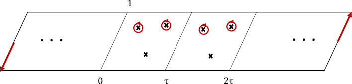
Figure 1: Integration contour $\mathcal{C}_{R}^{\eta}$ for $p>0$ in the rank-one case. The contour in the bulk is determined by the JK residue. Two vertical segments represent the potential singularities at $u=\rightarrow\pm\tau\infty$.

The integrand (5.7) transforms as:

$$I_{\mathfrak{m}}(u+k\tau,\nu)={\Pi}(u,\nu)^{-kp}\,I_{\mathfrak{m}}(u,\nu)=I_{\mathfrak{m}-kp}(u,\nu)~{},\qquad\qquad\forall k\in\mathbb{Z}~{},$$ (5.10)

under large gauge transformations (5.5) along $S^{1}_{\beta_{1}}$, with ${\Pi}$ the gauge flux operator. This directly follows from the properties of the fibering operator $\mathcal{F}_{1}$ for a non-anomalous gauge theory. Using this relation, we can write: 

$$\sum_{\mathfrak{m}\in\mathbb{Z}_{p}}\oint_{\mathcal{C}_{R}^{\eta}}\frac{dx}{2\pi ix}I_{\mathfrak{m}}(u,\nu) =\frac{1}{|W|}\sum_{k\in\mathbb{Z}}\sum_{\mathfrak{m}\in\mathbb{Z}_{p}}\int_{\mathcal{C}^{\eta}_{k}}du\;I_{\mathfrak{m}}(u,\nu)$$ (5.11)

$$=\frac{1}{|W|}\sum_{k\in\mathbb{Z}}\sum_{\mathfrak{m}\in\mathbb{Z}_{p}}\int_{\mathcal{C}^{\eta}_{0}}du\;I_{\mathfrak{m}-kp}(u,\nu)$$

$$=\frac{1}{|W|}\sum_{\mathfrak{m}\in\mathbb{Z}}\int_{\mathcal{C}^{\eta}_{0}}du\;I_{\mathfrak{m}}(u,\nu)~{}.$$

Here, we defined $\mathcal{C}_{k}^{\eta}$ the contour $\mathcal{C}^{\eta}$ restricted to the region $a_{1}\in[k,(k+1)]$, such that:

$$\mathcal{C}^{\eta}_{R}=\sum_{k\in\mathbb{Z}}\mathcal{C}^{\eta}_{k}~{},$$ (5.12)

as depicted in Figure 2. The contour $\mathcal{C}_{0}^{\eta}$ in the last expression is the “JK-contour” restricted to the fundamental domain of the torus. Generalizing to higher rank, we expect similar boundary contributions [27], and we conjecture a formula:

$$\mathcal{Z}_{\mathcal{M}_{g,p}\times S^{1}}(\mu_{i},s_{i})=\frac{1}{|W|}\sum_{\mathfrak{m}\in\mathbb{Z}^{{\rm rk}(\mathfrak{g})}}\int_{\mathcal{C}^{\eta}_{0}}\prod_{a=1}^{{\rm rk}(\mathfrak{g})}du_{a}\;I_{\mathfrak{m}}(u,\nu)~{},$$ (5.13)

In the case $p=0$, the boundary contributions are trivial, and (5.13) agrees with the formula for the $\Sigma_{g}\times T^{2}$ partition function in [19].

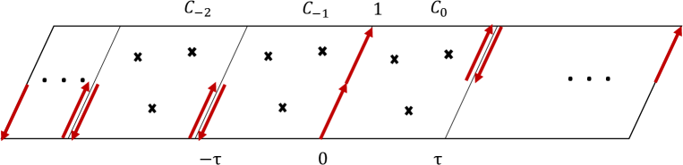
Figure 2: Decomposition of the boundary integral $\mathcal{C}^{\eta}_{R}=\sum_{k\in\mathbb{Z}}\mathcal{C}^{\eta}_{k}$. By an appropriate choice of the $R$-charges and of $\eta$, the contour in the bulk cancel each other and only the unit circle contour $a_{1}=0$ remains.

More generally, the manipulation (5.11) brings the $\mathcal{M}_{g,p}\times S^{1}$ partition function (5.6) to a form analogous to the $p=0$ case, including the sum over all gauge fluxes on $\Sigma_{g}$ in (5.13). At the level of these integral formulas, this simply corresponds to the relation (1.16) between spaces of different topologies.

5.2.1 The $W$-boson contribution.

The above analysis holds with one very important caveat. So far, we did not mention the potential singularities of the integrand (5.7) originating from poles in the one-loop determinant for the $W$-bosons, for any $\mathbf{G}$ non-abelian. Such $W$-bosons singularities exist if and only if $g>1$.

A deeper study of this important issue, which would lead to a more rigorous supersymmetric localization argument in the UV, is beyond the scope of this paper. For our purposes, it will be enough to note that the Bethe-vacua result can be obtained by naively summing over topological sectors with a JK residue that includes the matter chiral multiplets singularities only (plus contributions from the boundary), thus obtaining a naive sum over Bethe vacua of the abelianized theory, and then excluding by hand the would-be Bethe vacua not acted on freely by the Weyl group, as in [19].

5.3 The unit-circle contour integral

Starting from the formula (5.6) for $p\neq 0$, we can also deform the contour $\mathcal{C}^{\eta}$ to a simpler one, which can be related to previous results in the literature [2, 12]. Under a certain assumption on the flavor and R-symmetry backgrounds, which we will specify below, and for a suitable choice of $\eta$ for each $k$, we claim that:

$$\mathcal{C}^{\eta}\cong\sum_{k\in\mathbb{Z}^{{{\rm rk}(\mathfrak{g})}}}\mathcal{C}^{\eta(k)}_{k}\cong\prod_{a}\mathbb{T}_{x_{a}}~{},$$ (5.14)

where $\mathbb{T}_{x_{a}}$ is the unit circle in the $x_{a}$-plane, where $x_{a}=e^{2\pi iu_{a}}$. This correspond to an integration over flat connections $a_{2}$ over the $S^{1}$ in $\mathcal{M}_{g,p}\times S^{1}$. Interestingly, this is also the “naive” localization result one would obtain by imposing the standard reality conditions for the fields, so that we localize on four-dimensional flat connections, $F_{\mu\nu}=0$—see in particular [12]. For $p\neq 0$, such flat connections include the connections of non-trivial flat torsion bundles (5.3), which we sum over.

For the rank-one case, the equivalence (5.14) can be shown by taking:

$$\eta(k)>0\text{ for }k\geq 0~{},\quad\text{ and }\quad\eta(k)<0\text{ for }k<0.$$ (5.15)

Then, as illustrated in Figure 2, all the vertical segments in the bulk cancel each other except for the contour at $a_{1}=0$. The two boundary segments at either end do not contribute, because the integrand vanishes as we take them to infinity. There remain potential bulk contributions, but we claim that these do not contribute when a certain condition—see (5.25) below—holds. The remaining contour is precisely the unit circle contour (5.14). We claim that the equivalence holds for the higher-rank theories as well. We then have:

$$\mathcal{Z}_{\mathcal{M}_{g,p\neq 0}\times S^{1}}(y)=\frac{1}{|W_{\mathbf{G}}|}\sum_{\mathfrak{m}\in\mathbb{Z}_{p}^{{\rm rk}(\mathfrak{g})}}\oint_{\prod_{a}\mathbb{T}_{x_{a}}}\prod_{a=1}^{{{\rm rk}(\mathfrak{g})}}\frac{dx_{a}}{2\pi ix_{a}}\,I_{\mathfrak{m}}(x,y)~{},$$ (5.16)

where we wrote the integrand (5.7) as a function of $x_{a}$ and $y_{\alpha}=e^{2\pi i\nu_{\alpha}}$.

We can also argue for the formula (5.16) by directly relating it to the Bethe-vacua formula (3.11). This argument is analogous to the one in [27] for the three-dimensional $\mathcal{M}_{g,p}$ partition function. Let us again consider the rank-one case, for simplicity. Starting from (5.16), we may perform the sum over $\mathfrak{m}$ explicitly:

$$\sum_{\mathfrak{m}=0}^{p-1}I_{\mathfrak{m}}(x,y)={1-{\Pi}(x,y)^{p}\over 1-{\Pi}(x,y)}\,\mathcal{F}_{1}(x,y)^{p}\,\mathcal{H}(x,y)^{g-1}\,H(x,y)~{}.$$ (5.17)

Here and in the following, ${\Pi}$ is the gauge flux operator, while we omitted the flavor flux operators ${\Pi}_{\alpha}$ to avoid clutter. Using the difference equation ${\Pi}_{u}(x,y)\mathcal{F}_{1}(x,y)=\mathcal{F}(q^{-1}x,y)$, we can rewrite (5.16) as:

$$\mathcal{Z}_{\mathcal{M}_{g,p\neq 0}\times S^{1}} = \,\frac{1}{|W_{\mathbf{G}}|}\int_{|x|=1}{dx\over 2\pi ix}\,{\mathcal{F}_{1}(x,y)^{p}-\mathcal{F}_{1}(q^{-1}x,y)^{p}\over 1-{\Pi}(x,y)}\mathcal{H}(x,y)^{g-1}\,H(x,y)$$ (5.18)

$$= \,\frac{1}{|W_{\mathbf{G}}|}\int_{\Delta}{dx\over 2\pi x}\,{I_{0}(x,y)\over 1-{\Pi}(x,y)}~{},$$

where $I_{0}(x,y)$ is the integrand (5.7) at $\mathfrak{m}=0$. Here, $\Delta$ is the difference of the contour at $|x|=1$ and the contour at $|x|=|q|^{-1}$. Here we have used the fact that all factors in the integrand, apart from $\mathcal{F}(x,y)$, are invariant under $x\rightarrow qx$. As noted above, this relies on the absence of any anomalies for the gauge symmetry.

This contour integral is equal to the sum of the residues of all poles contained in the region $1<|x|<|q|^{-1}$. These poles may come from the numerator or denominator. However, we claim that, if we assume the relation (5.25) below, there are no poles in this region coming from the numerator. We will argue for this momentarily. Assuming it is true, the only poles in (LABEL:contrw) that lie inside this region are those at ${\Pi}(x,y)=1$. These are precisely the solutions to the “naive” Bethe equation (including, potentially, non-abelian vacua that one should discard). We thus find:

$$\mathcal{Z}_{\mathcal{M}_{g,p}\times S^{1}}(y)=-\frac{2\pi i}{|W_{\mathbf{G}}|}\sum_{\hat{x}\;|\;{\Pi}(\hat{x},y)=1}\text{Res}_{x=\hat{x}}\frac{\mathcal{F}(x,y)^{p}\mathcal{H}(x,y)^{g-1}H(x,y)}{1-\Pi(x,y)}~{}.$$ (5.19)

Using (2.67), one finds the residue of the $\frac{1}{1-\Pi}$ factor cancels the factor of $H$, and therefore:

$$-2\pi i\text{Res}_{x=\hat{x}}\frac{\mathcal{F}(x,y)^{p}\mathcal{H}(x,y)^{g-1}H(x,y)}{1-\Pi(x,y)}=\mathcal{F}(\hat{x},y)^{p}\mathcal{H}(\hat{x},y)^{g-1}~{}.$$ (5.20)

A similar argument holds for higher-rank theories. The acceptable Bethe solutions $\{\hat{x}_{a}\}$ to ${\Pi}_{a}(\hat{x},y)=1$ come in Weyl-group orbits of maximal size $|W_{\mathbf{G}}|$, canceling the Weyl-symmetry factor in (5.19). The contribution from the non-acceptable solutions, which are not acted on freely by the Weyl group, should be discarded by hand. Reinstating the flavor flux operators, this leaves us with:

$$\mathcal{Z}_{\mathcal{M}_{g,p}\times S^{1}}(y)=\sum_{\hat{x}\in\mathcal{S}_{BE}}\mathcal{F}(\hat{x},y)^{p}\,\mathcal{H}(\hat{x},y)^{g-1}\,{\Pi}_{\alpha}(\hat{x},y)^{\mathfrak{n}_{\alpha}}~{},$$ (5.21)

which is precisely the sum-over-Bethe-vacua formula (3.11).

In this sense, the relation between the integral formula and the Bethe-vacua formula is only formal, as we already anticipated. For $g=0$, the contribution from the non-acceptable Bethe vacua vanishes, because $\mathcal{H}^{-1}$ vanishes on such solutions—for $g>1$, on the other hand, it would diverge. Since the Bethe-vacua formula has a rather simple derivation and itself passes a number of physical consistency checks, the open challenge would be to specify the exact contour $\mathcal{C}^{\eta}$ in (5.6), valid for any $g>0$, that reproduces the Bethe-vacua answer without further assumption. We leave this for future work.

This important remark notwithstanding, it remains to derive the conditions under which there are no poles coming from the numerator in (LABEL:contrw). Apart from the Hessian factor, a single chiral multiplet of gauge charge $Q$ and $R$-charge $r$ contributes to this numerator as:

$$Z^{\Phi}_{\mathfrak{m}=0}(x) = \;\mathcal{F}^{\Phi}(x^{Q}y)^{p}\,\Pi^{\Phi}(x^{Q}y)^{\mathfrak{n}+(r-1)(g-1)}$$ (5.22)

$$\sim \;\prod_{m\in\mathbb{Z}}\left[1\over 1-q^{m}x^{Q}y\right]^{pm+\mathfrak{n}+(r-1)(g-1)}~{},$$

in the $A$-twist gauge—see Appendix C.2. Here, $y$ and $\mathfrak{n}$ are the net flavor parameters the chiral multiplet couples to. This expression can have a pole when $x^{Q}=y^{-1}q^{-m}$ for some $m\in\mathbb{Z}$. In addition, the chiral multiplet contributes a simple pole at the same points to the Hessian determinant, $H(x)$. Generically, this is the only source of a pole at this point, so the behavior of the numerator $I_{0}(x)$ here is given by:

$$I_{0}(x)\underset{x^{Q}\sim y^{-1}q^{-m}}{\sim}Z^{\Phi}_{\mathfrak{m}=0}(x)\,H(x)^{g}\sim(1-q^{n}x^{Q}y)^{-(pm+\mathfrak{n}+(r-1)(g-1)+g)}~{}.$$ (5.23)

Let us fix $p>0$, for definiteness. Picking $m$ so that the exponent is negative, one finds that a pole can only arise when:

$$|x|^{Q}\geq|y|^{-1}|q|^{{\mathfrak{n}+r(g-1)\over p}}~{}.$$ (5.24)

Now, we want to impose that there are no poles of the integrand (LABEL:contrw) coming from $I_{0}$, in the region $1<|x|<|q|^{-1}$, for this chiral multiplet. For $Q<0$, we should pick the parameters so that the RHS of (5.24) is bounded below by $1$. For $Q>0$, we would naively bound the RHS below by $|q|^{-Q}$; however, since the denominator of (LABEL:contrw) also blows up at these points, we may actually allow sufficiently mild poles in the numerator, and one finds that RHS need only be bounded below by $1$. Summarizing, in either case, we find the condition:

$$|y|\;|q|^{-{\mathfrak{n}+r(g-1)\over p}}<1~{}.$$ (5.25)

If we impose this relation for all the chiral multiplets in the theory, then the numerator contributes no poles at all to (LABEL:contrw), and this completes the proof. The restriction (5.25) implies that we may only perform this calculation in some subset of parameter space, and this may not be compatible with the physical constraints imposed by the superpotential and anomaly cancellation. However, having performed the computation here, we may then extend it to the rest of parameter space by analytic continuation. Moreover, by starting in such a region of parameter space and continuously varying parameters, one may deform the contour such that it is not crossed by any poles, and one may, in principle, obtain the correct integration contour for any point in parameter space in this way. The argument for higher rank is a straightforward extension [27].

An interesting special case of (5.25) is when we consider real chemical potentials only, so that $|y|=1$. In that case, the condition is simply that $\mathfrak{n}+r(g-1)<0$. In particular, on the three-sphere with $\mathfrak{n}=0$, we simply need all the chiral multiplet $R$-charges to be positive, $r>0$.

5.4 The three-sphere supersymmetric index

In the case $\mathcal{M}_{g,p}=S^{3}$, we may also work in the physical gauge and at real $R$-charges, $r\in\mathbb{R}$, as explained in section 4. Consider the physical gauge for any $\mathcal{M}_{g,p}$ such that (4.3) holds. The chiral multiplet one-loop determinant can have poles at $x^{Q}=y^{-1}q^{-m-l_{R}(r-1)}$, with $l_{R}$ defined in (4.10), for $m$ such that $pm+\mathfrak{n}>0$. By the same reasoning as above for $p>0$, this leads us to the same condition as in (5.25), with the difference that $r$ can be real. In particular, for $S^{3}$, we should have:

$$|y_{i}|\;|q|^{r_{i}}<1~{},$$ (5.26)

for every chiral multiplet $\Phi_{i}$. The integral formula (5.16) then reads:

$$\mathcal{Z}^{\rm phys}_{S^{3}\times S^{1}}(y;q)=\frac{1}{|W_{\mathbf{G}}|}\oint_{\prod_{a}\mathbb{T}_{x_{a}}}\prod_{a=1}^{{{\rm rk}(\mathfrak{g})}}\frac{dx_{a}}{2\pi ix_{a}}\,\mathcal{F}_{1}^{\rm phys}(x,y;q)~{},$$ (5.27)

where we have a single topological sector because $p=1$. The integrand is the “physical” fibering operator (LABEL:physical_fibering_op_G) for $\nu_{R}=\tau$. Once we strip away the supersymmetric Casimir energy term,

$$\mathcal{Z}^{\rm phys}_{S^{3}\times S^{1}}(y;q)=q^{E_{S^{3}}}\,\mathcal{I}_{S^{3}}^{\rm phys}(y;q)~{},$$ (5.28)

with $E_{S^{3}}$ given by the first equality in (LABEL:Casimir_E_phys) with $\nu_{R}=\tau$, we are left with the index formula:

$$\mathcal{I}_{S^{3}}^{\rm phys}(y;q)=\frac{(q;q)^{2{{\rm rk}(\mathfrak{g})}}_{\infty}}{|W_{\mathbf{G}}|}\oint_{\prod_{a}\mathbb{T}_{x_{a}}}\prod_{a=1}^{{{\rm rk}(\mathfrak{g})}}\frac{dx_{a}}{2\pi ix_{a}}\,{\prod_{i}\prod_{\rho_{i}}\Gamma_{0}\big{(}\rho_{i}(u)+\nu_{i}+\tau(r_{i}-1);\tau\big{)}\over\prod_{\alpha\in\mathfrak{g}}\Gamma_{0}\big{(}\alpha(u)-\tau;\tau\big{)}}~{},$$ (5.29)

with $y=e^{2\pi i}$, $q=e^{2\pi i\tau}$. This is the standard expression for the $S^{3}$ supersymmetric index [2, 34] with ${\bf p}={\bf q}=q$. From (5.26), we see that this formula is valid, in particular, for real chemical potentials $\nu_{i}$ and positive $R$-charges, $r_{i}>0$. The contour integral in (5.29) has a standard interpretation as a projection onto gauge-invariant states. For more general parameters, we can deform the contour appropriately, as mentioned above.

Finally, we note that our simple proof of the equality between the integral formula and the Bethe-vacua formula goes through without problem, so that (5.29) is exactly equal to (4.32).

6 Supersymmetric dualities

The exact computation of supersymmetric partition functions can provide detailed evidence for supersymmetric dualities. In this section, we compute the $\mathcal{M}_{g,p}\times S^{1}$ partition function for dual pairs of four-dimensional gauge theories, using the Bethe-equation approach. We focus on Seiberg dualities between $\mathcal{N}=1$ gauge theories with $USp(2N_{c})$ and $SU(N_{c})$ gauge groups. We verify that the dual partition functions agree. This new test of Seiberg duality can also be viewed as a strong consistency check of our general results.

6.1 Generalities: Mapping Bethe vacua and surface operators

Before turning to the examples, let us make a few general comments, closely following the three-dimensional discussion of [27]. Consider some gauge theory $\mathcal{T}$. We know from (3.11) that we may write the $\mathcal{M}_{g,p}\times S^{1}$ partition function as:

$$\mathcal{Z}_{\mathcal{M}_{g,p}\times S^{1}}(\nu,n)=\sum_{\hat{u}\in\mathcal{S}_{\rm BE}}\mathcal{F}_{1}(\hat{u},\nu)^{p}\,\mathcal{H}(\hat{u},\nu)^{g-1}\,{\Pi}_{\alpha}(\hat{u},\nu)^{\mathfrak{n}_{\alpha}}~{},$$ (6.1)

where $\nu_{\alpha}$ and $\mathfrak{n}_{\alpha}$ are the flavor fugacities and background fluxes, respectively. (The geometric parameter $\tau$ is kept implicit.) If the theory has an infrared-dual description as another gauge theory, $\mathcal{T}^{D}$, one may write the dual partition function similarly:

$$\mathcal{Z}_{\mathcal{M}_{g,p}\times S^{1}}^{D}(\nu,n)=\sum_{\hat{u}^{D}\in\mathcal{S}^{D}_{\rm BE}}\mathcal{F}_{1}^{D}(\hat{u}^{D},\nu)^{p}\,\mathcal{H}^{D}(\hat{u}^{D},\nu)^{g-1}\,{\Pi}^{D}_{\alpha}(\hat{u}^{D},\nu)^{\mathfrak{n}_{\alpha}}~{}.$$ (6.2)

Here we assumed that the dual gauge theories have isomorphic flavor symmetries,  and we identified the flavor parameters appropriately. To prove the equality of supersymmetric partition functions, on any four-manifold $\mathcal{M}_{g,p}\times S^{1}$ and for any set of flavor symmetry background fluxes, it suffices to exhibit a “duality map” between the two-dimensional Bethe vacua, such that dual operators are equal when evaluated on dual vacua. More precisely, we must find a bijection:

$$\mathcal{D}\;:\;\;\mathcal{S}_{BE}\rightarrow\mathcal{S}_{BE}^{D}\;\;:\;\;\{\hat{u}\}\mapsto\{\hat{u}^{D}\}~{},$$ (6.3)

such that:

$$\mathcal{F}_{1}(\hat{u},\nu)=\mathcal{F}_{1}(\hat{u}^{D},\nu)~{},\qquad\mathcal{H}(\hat{u},\nu)=(-1)^{s(\Delta\mathcal{H})}\,\mathcal{H}(\hat{u}^{D},\nu)~{},$$ (6.4)

for the fibering and handle-gluing operators, and

$${\Pi}_{\alpha}(\hat{u},\nu)=(-1)^{s({\Pi}_{\alpha})}\,{\Pi}_{\alpha}(\hat{u}^{D},\nu)$$ (6.5)

for the flavor flux operators. The matching of these operators in every supersymmetric vacuum immediately implies the equality

$$\mathcal{Z}_{\mathcal{M}_{g,p}\times S^{1}}(\nu,n)=(-1)^{(g-1)s(\mathcal{H})+\mathfrak{n}_{\alpha}s({\Pi}_{\alpha})}\;\mathcal{Z}_{\mathcal{M}_{g,p}\times S^{1}}^{D}(\nu,n)$$ (6.6)

for the partition function. Note that the duality relation (6.4) for the fibering operator implies (6.5), due to the difference equations (LABEL:ell_F1), and the fact that ’t Hooft anomalies must match between dual theories. Similarly, the matching of $\mathcal{F}_{1}$ also implies the matching of the other fibering operator, $\mathcal{F}_{1}(\hat{u})=\mathcal{F}^{D}_{1}(\hat{u}^{D})$, since the two fibering operators are related by (2.62).

Note the appearance of subtle signs $(-1)^{s(\mathcal{H})}$ and $(-1)^{s({\Pi}_{\alpha})}$ in the duality relations. They are given explicitly by:

$$s(\mathcal{H})\equiv{1\over 2}\left(\mathcal{A}^{RR}-\mathcal{A}^{RR}_{D}\right)-\dim(\mathbf{G})+\dim(\mathbf{G}^{D})\;\qquad({\rm mod}\;2)~{},$$ (6.7)

$$s({\Pi}_{\alpha})\equiv{1\over 2}\left(\mathcal{A}^{\alpha\alpha}-\mathcal{A}^{\alpha\alpha}_{D}\right)\;\qquad({\rm mod}\;2)~{},$$

with $\mathbf{G}$ and $\mathbf{G}^{D}$ the gauge groups of the dual theories $\mathcal{T}$ and $\mathcal{T}^{D}$, respectively. Here $\mathcal{A}^{RR}$ and $\mathcal{A}^{\alpha\beta}$ are the quadratic “pseudo-anomalies”:

$$\mathcal{A}^{RR}=\sum_{I}(r_{I}-1)^{2}+\dim(\mathbf{G})~{},\qquad\qquad\mathcal{A}^{\alpha\alpha}=\sum_{I}Q_{I}^{\alpha}Q_{I}^{\alpha}~{},$$ (6.8)

and similarly for $\mathcal{A}^{RR}_{D}$ and $\mathcal{A}^{\alpha\alpha}_{D}$ in the dual theory. One can show that $s(\mathcal{H})$ and $s({\Pi}_{\alpha})$ are integers. The sign $(-1)^{s({\Pi}_{\alpha})}$ follows from the equality of the dual fibering operators together with the second line in (LABEL:ell_F1), and the sign $(-1)^{s(\mathcal{H})}$ can be similarly determined by consistency. We find that the relative sign in (6.6) is given in terms of the quadratic “pseudo-anomalies”, but the physical meaning of this observation is unclear.  In particular, we should note that trivial modifications of the UV completion of a theory, such as the inclusion of very massive fields charged under the flavor symmetry, can modify the sign of the $A$-model partition function. We leave a more thorough understanding of this point for future work.

To conclude with our general remarks, we would like to emphasize that the duality map (6.3) allows us to map any pairs of operators in the dual four-dimensional A-models—in principle. That is, we may consider the expectation values of any half-BPS surface operators $\mathcal{S}$ wrapping the torus fiber, which are computed by insertions the corresponding $A$-model operator $\mathcal{S}(u,\nu)$ in the sum over Bethe vacua. We have:

$$\langle\mathcal{S}\rangle_{\mathcal{M}_{g,p}\times S^{1}}=\sum_{\hat{u}\in\mathcal{S}_{\rm BE}}\mathcal{S}(\hat{u},\nu)\,\mathcal{F}_{1}(\hat{u},\nu)^{p}\,\mathcal{H}(\hat{u},\nu)^{g-1}\,{\Pi}_{\alpha}(\hat{u},\nu)^{\mathfrak{n}_{\alpha}}~{},$$ (6.9)

for the unnormalized expectation value—or correlation functions, since these correlators are independent of the insertion points—, and similarly for surface operators in the dual theory. Thus, if we can find a pair of dual surface operators, which must satisfy:

$$\mathcal{S}(\hat{u},\nu)=\mathcal{S}^{D}(\hat{u}^{D},\nu)$$ (6.10)

in all Bethe vacua, we may also infer the equality of their expectation values on $\mathcal{M}_{g,p}\times S^{1}$ in the dual theories.

6.2 Example: $\mathcal{N}=1$ $SU(2)$ gauge theory with $N_{f}$ flavors

Before discussing some larger families of dualities, we pause here to describe the computation of the $\mathcal{M}_{g,p}\times S^{1}$ partition function in a simple example. This serves to make some of the abstract considerations above more concrete. The example we consider will be the $\mathcal{N}=1$ $SU(2)$ gauge theory with $N_{f}$ flavors, i.e. $2N_{f}$ chiral multiplets in the fundamental representation of $SU(2)$.  Let us introduce the parameters $u$ for the Cartan of the $SU(2)$ gauge symmetry, and $\nu_{i}$, $i=1,\cdots,2N_{f}$, for that of the $SU(2N_{f})$ flavor symmetry, which satisfy $\sum_{i=1}^{2N_{f}}\nu_{i}=0$. The twisted superpotential of this theory reads:

$$\mathcal{W}(u,\nu)=\sum_{i=1}^{2N_{f}}\big{(}\mathcal{W}_{\Phi}(u+\nu_{i};\tau)+\mathcal{W}_{\Phi}(-u+\nu_{i};\tau)\big{)}~{}.$$ (6.11)

As usual, there is no contribution from the W-bosons.

$A$-model operators and Bethe vacua.

From the twisted superpotential, we may construct the gauge flux operators:

$$\Pi_{u}=e^{2\pi i\partial_{u}\mathcal{W}}=\prod_{i=1}^{2N_{f}}\frac{\Pi^{\Phi}(u+\nu_{i})}{\Pi^{\Phi}(-u+\nu_{i})}=\prod_{i=1}^{2N_{f}}\frac{\theta(-u+\nu_{i};\tau)}{\theta(u+\nu_{i};\tau)}~{},$$ (6.12)

the flavor flux operators:

$$\Pi_{i}=e^{2\pi i\partial_{\nu_{i}}\mathcal{W}}=\frac{e^{\frac{\pi i}{\tau}(u^{2}+{\nu_{i}}^{2})}}{\theta(u+\nu_{i};\tau)\theta(-u+\nu_{i};\tau)}~{},$$ (6.13)

the fibering operator:

$$\mathcal{F}_{1}=\prod_{i=1}^{2N_{f}}\mathcal{F}^{\Phi}_{1}(u+\nu_{i})\mathcal{F}^{\Phi}_{1}(-u+\nu_{i})=e^{\frac{2\pi i}{3\tau^{2}}\sum_{i=1}^{2N_{f}}{\nu_{i}}^{3}}\prod_{i=1}^{2N_{f}}\Gamma_{0}(u+\nu_{i};\tau)\Gamma_{0}(-u+\nu_{i};\tau)~{},$$ (6.14)

and the handle-gluing operator:

$$\mathcal{H}=H\prod_{i=1}^{2N_{f}}\Big{[}e^{\frac{2\pi i}{\tau}{\nu_{i}}^{2}}\theta(u+\nu_{i};\tau)\theta(-u+\nu_{i};\tau)\Big{]}^{1-r_{j}}\;\frac{1}{\eta(\tau)^{2}}\,\frac{1}{\theta(2u;\tau)\theta(-2u;\tau)}~{},$$ (6.15)

where:

$$H=\frac{\partial^{2}\mathcal{W}}{\partial u^{2}}=-{1\over 2\pi i}\sum_{i=1}^{2N_{f}}\bigg{(}\frac{\theta^{\prime}(u+\nu_{i};\tau)}{\theta(u+\nu_{i};\tau)}+\frac{\theta^{\prime}(-u+\nu_{i};\tau)}{\theta(-u+\nu_{i};\tau)}\bigg{)}~{}.$$ (6.16)

More precisely, each flux operator $\Pi_{i}$ by itself corresponds to an anomalous symmetry. The non-anomalous $SU(2N_{f})$ flux insertions are:

$${\Pi}_{SU(2N_{f})}=\prod_{i=1}^{2N_{f}}{{\Pi}_{i}}^{\mathfrak{n}_{i}},\;\;\;\;\quad\text{such that}\qquad\sum_{i=1}^{2N_{f}}\mathfrak{n}_{i}=0~{}.$$ (6.17)

Then, ${\Pi}_{SU(2N_{f})}$ is an elliptic function of $u$. For the handle-gluing operator, we must pick a non-anomalous R-symmetry by assigning the chiral multipets R-charges $r_{j}\in\mathbb{Z}$ satisfying the anomaly-free condition:

$$\mathcal{A}^{uuR}=\sum_{i=1}^{2N_{f}}(r_{i}-1)+4=0~{}.$$ (6.18)

The vacua of the theory are determined by the Bethe equation:

$${\Pi}_{u}=\prod_{i=1}^{2N_{f}}\frac{\theta(-u+\nu_{i};\tau)}{\theta(u+\nu_{i};\tau)}=1~{}.$$ (6.19)

As described in more detail in the next subsection, for generic $\nu_{i}$, this has $2N_{f}$ solutions in a given fundamental domain of the torus:

$$\hat{u}\in\{0,-\frac{1}{2},-\frac{\tau}{2},\frac{1+\tau}{2}\}\cup\{\hat{u}_{l},-\hat{u}_{l}\},\;\;\;l=1,\cdots,N_{f}-2~{},$$ (6.20)

for some $\hat{u}_{l}$ depending on the $\nu_{i}$’s. A solution corresponding to a valid vacuum must be acted freely by the Weyl symmetry, $\hat{u}\rightarrow-\hat{u}$, which excludes the first four solutions in (6.20), and solutions are considered up to this symmetry, so the set of Bethe vacua is:

$$\mathcal{S}_{BE}=\{\hat{u}_{l},\;\;\;l=1,\cdots,N_{f}-2\}$$ (6.21)

In particular, this theory has $N_{f}-2$ massive vacua when quantized on a torus with generic flavor fugacities $\nu$. That is, we find the Witten index:

$$\mathcal{Z}_{T^{4}}=N_{f}-2~{}.$$ (6.22)

Bethe sum formula for the partition function.

The $\mathcal{M}_{g,p}\times S^{1}$ partition function is given by:

$$\mathcal{Z}_{\mathcal{M}_{g,p}\times S^{1}}(\nu)=\sum_{l=1}^{N_{f}-2}\mathcal{F}_{1}(\hat{u}_{l},\nu)^{p}\,\mathcal{H}(\hat{u}_{l},\nu)^{g-1}\,{\Pi}_{i}(\hat{u}_{l},\nu)^{\mathfrak{n}_{i}}~{},$$ (6.23)

where the sum runs over the supersymmetric vacua in (6.21), and the dependence on $\tau$ is implicit. In practice, it may be difficult to compute (6.23) explicitly since we only know the $\hat{u}_{l}$ implicitly through (6.19). One way to proceed is by working perturbatively in $q=e^{2\pi i\tau}$. We use the exponentiated variables, $x=e^{2\pi iu}$ and $y_{i}=e^{2\pi i\nu_{i}}$, and expand:

$${\Pi}_{u}={\Pi}_{u}^{(0)}+q{\Pi}_{u}^{(1)}+\cdots,\;\;\;\;\;\hat{x}_{l}={\hat{x}_{l}}^{(0)}+q{\hat{x}_{l}}^{(1)}+\cdots$$ (6.24)

Then the ${\hat{x}_{l}}^{(0)}$ are given by solutions to the polynomial equation:

$${\Pi}_{u}^{(0)}=\prod_{i=1}^{2N_{f}}\frac{x-y_{i}}{1-xy_{i}}=1\qquad\Leftrightarrow\qquad\prod_{i=1}^{2N_{f}}(x-y_{i})-\prod_{i=1}^{2N_{f}}(1-xy_{i})=0~{}.$$ (6.25)

One can then correct these solutions order by order in $q$. For example, one finds that the leading correction is given by: 

$$\hat{z}_{l}\equiv\hat{x}_{l}+{\hat{x}_{l}}^{-1}=\hat{z}_{l}^{(0)}+q\;\frac{\big{(}{\mbox{$\hat{z}_{l}$}^{(0)}}^{2}-4\big{)}\displaystyle\sum_{i=1}^{2N_{f}}(y_{i}-{y_{i}}^{-1})}{\displaystyle\sum_{i=1}^{2N_{f}}\frac{y_{i}-{y_{i}}^{-1}}{y_{i}+{y_{i}}^{-1}-{\mbox{$\hat{z}_{l}$}^{(0)}}}}+O(q^{2})~{}.$$ (6.26)

One can systematically compute higher order corrections in a similar way; however, this quickly becomes quite cumbersome to do analytically.

The $N_{f}=3$ case.

For concreteness, let us consider in more detail the case $N_{f}=3$. In this case, there is a single Bethe vacuum, up to the Weyl symmetry, and one computes the leading order solution:

$$\hat{z}^{(0)}=\frac{\sum_{i<j}(y_{i}y_{j}-{y_{i}}^{-1}{y_{j}}^{-1})}{\sum_{i}(y_{i}-{y_{i}}^{-1})}~{},\qquad\text{if}\quad N_{f}=3~{}.$$ (6.27)

One can use (6.26) to compute the solution to the next order in $q$.

We can use this solution to compute the $\mathcal{M}_{g,p}\times S^{1}$ partition function to leading order in $q$. Let us assume, for simplicity, that the flavor symmetry fluxes vanish, $\mathfrak{n}_{i}=0$. Then, we simply need evaluate the fibering and handle-gluing operators at the Bethe solution. For general $N_{f}$ (writing $\hat{z}=\hat{x}+{\hat{x}}^{-1}$ as above, and stripping off the Casimir energy factors for simplicity), we find:

$$\mathcal{F}_{1}=1+q\hat{z}\sum_{i=1}^{2N_{f}}\big{(}y_{i}-{y_{i}}^{-1}\big{)}+O(q^{2})~{},$$ (6.28)

$$\mathcal{H}=H\frac{\prod_{i=1}^{2N_{f}}(y_{i}+{y_{i}}^{-1}-\hat{z})^{1-r_{i}}}{\hat{y}^{2}-4}$$

$$\qquad\qquad\times\bigg{(}1+q\big{(}2\hat{z}^{2}-2+\sum_{i=1}^{2N_{f}}(r_{i}-1)\hat{z}(y_{i}+{y_{i}}^{-1})\big{)}\bigg{)}+O(q^{2})~{},$$

with

$$H=\sum_{j=1}^{2N_{f}}\bigg{(}\frac{v_{j}-{v_{j}}^{-1}}{v_{j}+{v_{j}}^{-1}-\hat{y}}-q\hat{y}(v_{j}-{v_{j}}^{-1})\bigg{)}+O(q^{2})~{}.$$ (6.29)

After plugging in the form of $\hat{z}$ above, one eventually finds a relatively simple results for $N_{f}=3$ at first order in $q$:

$$\mathcal{F}_{1}=1+q\sum_{i<j}(y_{i}y_{j}-{y_{i}}^{-1}{y_{j}}^{-1})+O(q^{2})~{},$$ (6.30)

$$\mathcal{H}=\prod_{i=1}^{6}{y_{i}}^{2r_{i}}\prod_{i<j}(1-y_{i}y_{j})^{1-r_{i}-r_{j}}\bigg{(}1+q\sum_{i<j}(r_{i}+r_{j}-1)(y_{i}y_{j}+{y_{i}}^{-1}{y_{j}}^{-1})\bigg{)}+O(q^{2})~{}.$$

One can verify that these precisely agree with the leading order $q$-expansions of the fibering and handle-gluing operator for a theory of $15$ free chiral multiplets, which can be identified with the mesons, $Q_{i}Q_{j}$, of the $SU(2)$ $N_{f}=3$ theory. This gives a simple example of the duality of [41], with R-charges mapped appropriately across the duality. We will discuss this duality in more generality in the next subsection. The $\mathcal{M}_{g,p}\times S^{1}$ partition function is simply given by:

$$\mathcal{Z}_{\mathcal{M}_{g,p}\times S^{1}}={\mathcal{F}_{1}}^{p}\mathcal{H}^{g-1}$$ (6.31)

with $\mathcal{F}_{1}$ and $\mathcal{H}$ given, to leading order in $q$, by (LABEL:exos).

Integral formula

We may alternatively use the integral formulas in Section 5. Let us consider the case $p\neq 0$, so that we may use the formula (5.16), which gives:

$$\mathcal{Z}_{\mathcal{M}_{g,p}\times S^{1}}(y)=\frac{1}{2}\sum_{\mathfrak{m}\in{\mathbb{Z}_{p}}}\oint_{\mathbb{T}}\frac{dx}{x}\mathcal{F}(x,y)^{p}\,\mathcal{H}(x,y)^{g-1}\,H(x,y)\,{\Pi}_{u}(x,y)^{\mathfrak{m}}~{}.$$ (6.32)

We have argued in the previous section that this agrees with the known formula for the $S^{3}\times S^{1}$ index in the case $g=0$, $p=1$, but let us check this explicitly here. In this case, the above becomes:

$$\mathcal{Z}_{S^{3}\times S^{1}}(y)\;=\;\frac{1}{2}\oint_{\mathbb{T}}\frac{dx}{x}\mathcal{H}(x,y)^{-1}H(x,y)\mathcal{F}_{1}(x,y)$$

$$=\frac{1}{2}\oint_{\mathbb{T}}\frac{dx}{x}(x-x^{-1})^{2}\prod_{i=1}^{2N_{f}}(y_{i}+{y_{i}}^{-1}-x-x^{-1})^{r_{j}-1}\;\Bigg{[}1+q\;\bigg{[}(x+x^{-1})\sum_{j=1}^{2N_{f}}\big{(}y_{j}-{y_{j}}^{-1}\big{)}$$

$$\;\qquad\qquad\qquad\qquad-2(x+x^{-1})^{2}+2+\sum_{j=1}^{2N_{f}}(1-r_{j})(x+x^{-1})(y_{j}+{y_{j}}^{-1})\bigg{]}\Bigg{]}+O(q^{2})~{}.$$

Here, one must take care because the terms in the $q$-expansion are typically rational functions of $x$, rather than polynomials as in the superconformal $S^{3}\times S^{1}$ index.  To deal with these, we formally make the assumption (5.25), which imposes that the $|y_{i}|$ are small, which determines which poles are enclosed by the unit circle contour. Taking as an explicit example the anomaly-free R-charge assignments $\{r_{i}\}=\{0,0,0,0,1,1\}$, we find poles at $x={y_{i}}^{\pm}$, $i=1,...,4$, and taking those poles with the top sign, which lie inside the unit circle, one computes:

$$\mathcal{Z}_{S^{3}\times S^{1}}(y)=\frac{{y_{5}}^{2}{y_{6}}^{2}(1-y_{5}y_{6})}{\prod_{1\leq i<j\leq 4}(1-y_{i}y_{j})}\bigg{(}1+q\bigg{(}-y_{5}y_{6}-{y_{5}}^{-1}{y_{6}}^{-1}+\sum_{1\leq i<j\leq 4}(y_{i}y_{j}+{y_{i}}^{-1}{y_{j}}^{-1})$$ (6.33)

$$\qquad\qquad\qquad+\sum_{i<j}(v_{i}v_{j}-{v_{i}}^{-1}{v_{j}}^{-1})\bigg{)}\bigg{)}+O(q^{2})~{},$$

which one can check agrees with (6.31) in this case.

6.3 $USp(2N_{c})$ duality

Now let us consider the general duality of [41], which relates the following four-dimensional $\mathcal{N}=1$ gauge theories: 

• A gauge group $USp(2N_{c})$, with the vector multiplet coupled to $2N_{f}$ fundamental chiral multiplets $Q_{i}$.

• A gauge group $USp(2N_{f}-2N_{c}-4)$, with the vector multiplet coupled to $2N_{f}$ fundamental chiral multiplets $q^{i}$. In addition, the theory contains $N_{f}(2N_{f}-1)$ gauge-singlet chiral multiplets, denoted $M_{ij}$, $\scriptsize{1\leq i<j\leq 2N_{f}}$, which interact with the charged multiplets through the superpotential $W=M_{ij}q^{i}q^{j}$.

Both of these theories have an $SU(2N_{f})$ flavor symmetry. Note that the number of flavors is even in order to cancel the $USp(2N_{c})$ global anomaly. The charges of the chiral multiplets are summarized in Table 1. The gauge-singlet “mesons” $M_{ij}$ of the second theory, in the antisymmetric representation of $SU(2N_{f})$, are identified with the gauge-invariant mesons $Q_{i}Q_{j}$ in the first theory. The $R$-charges $r_{i}$ must satisfy:

$$\sum_{i=1}^{2N_{f}}(r_{i}-1)+2N_{c}+2=0~{},$$ (6.34)

in order to cancel the $U(1)_{R}$-(gauge)² anomaly. We may choose any $r_{i}\in\mathbb{Z}$ satisfying (6.34). Let us also introduce $\nu_{i}$ and $\mathfrak{n}_{i}$ the $SU(2N_{f})$ flavor chemical potential and fluxes, subject to the traceless condition:

$$\sum_{i=1}^{2N_{f}}\nu_{i}=0~{},\qquad\qquad\sum_{i=1}^{2N_{f}}\mathfrak{n}_{i}=0~{}.$$ (6.35)

6.3.1 ’t Hooft anomaly matching and relative signs

One of the earliest, non-trivial test of Seiberg duality was the matching of ’t Hooft anomalies [33, 41]. For $\mathbf{G}_{F}=SU(2N_{f})$, we have:

$$\mathcal{A}^{\alpha\beta\gamma}\nu_{\alpha}\nu_{\beta}\nu_{\gamma}=2N_{c}\sum_{i=1}^{2N_{f}}\nu_{i}^{3}~{},\qquad\quad\mathcal{A}^{R\,\alpha\beta}\nu_{\alpha}\nu_{\beta}=2N_{c}\sum_{i=1}^{2N_{f}}(r_{i}-1)\,\nu_{i}^{2}~{},$$ (6.36)

in the $USp(2N_{c})$ theory. It is easy to check that these anomalies are reproduced by the dual $USp(2N_{f}-2N_{c}-4)$ theory, given the relations (6.34) and (6.35). We can similarly check the matching of $\mathcal{A}^{R}$ and $\mathcal{A}^{RRR}$ across the duality. One can also check that the quadratic $SU(2N_{f})$ pseudo-anomaly vanishes (mod 4) in both theories. On the other hand, we have a non-trivial sign $(-1)^{s(\mathcal{H})}$ as defined by (LABEL:def_sCH_spif). One finds:

$$(-1)^{s(\mathcal{H})}=(-1)^{N_{c}+N_{f}+1}~{},\qquad\qquad(-1)^{s({\Pi}_{i})}=1~{},$$ (6.37)

with ${\Pi}_{i}$ the $SU(2N_{f})$ flux operators.

	$USp(2N_{c})$	$USp(2N_{f}-2N_{c}-4)$	$SU(2N_{f})$	$U(1)_{R}$
$Q_{i}$	${\bf 2N_{c}}$	$-$	${\bf 2N_{f}}$	$r_{i}$
$q^{i}$	$-$	${\bf 2(N_{f}-N_{c}-2)}$	$\overset{\vspace{1mm}}{\overline{\bf 2N_{f}}}$	$1-r_{i}$
$M_{ij}$	$-$	${\bf 1}$	${\bf N_{f}(2N_{f}-1)}$	$r_{i}+r_{j}$

Table 1: Charges for the $USp(2N_{c})$ theory its $USp(2N_{f}-2N_{c}-4)$ dual.

6.3.2 $USp(2N_{c})$ Bethe equations and duality map

To check the duality at the level of the A-model, we must first study the set of Bethe vacua in the two theories. Starting with the first theory, let $u_{a},\;a=1,\cdots,N_{c}$, denote the parameters for the Cartan of the gauge symmetry. The twisted superpotential is given by:

$$\mathcal{W}_{\Phi}(u,\nu)=\sum_{a=1}^{N_{c}}\sum_{i=1}^{2N_{f}}\big{(}\mathcal{W}_{\Phi}(u_{a}+\nu_{i})+\mathcal{W}_{\Phi}(-u_{a}+\nu_{i})\big{)}~{},$$ (6.38)

with $\mathcal{W}_{\Phi}(u)$ defined in (2.10). The corresponding Bethe equations are:

$$\exp\left(2\pi i{\partial\mathcal{W}\over\partial u_{a}}\right)={\Pi}_{0}(u_{a})=1~{},\;\;\qquad a=1,\cdots,N_{c}~{},$$ (6.39)

where we defined:

$${\Pi}_{0}(u)\equiv\prod_{i=1}^{2N_{f}}\frac{\theta(-u+\nu_{i})}{\theta(u+\nu_{i})}~{}.$$ (6.40)

Note that ${\Pi}_{0}(u)$ is an elliptic function of $u$. (It is also elliptic in the parameters $\nu_{i}$ modulo the traceless constraint.) Since ${\Pi}_{0}(u)-1$ has $2N_{f}$ poles in $u$, in a given fundamental domain, it must also have $2N_{f}$ distinct zeros, for generic values of the parameters. Let us denote these “Bethe roots” by $\tilde{u}_{k}$, $k=1,\cdots,2N_{f}$.

A Bethe vacuum is determined by an assignment of the $N_{c}$ eigenvalues $u_{a}$ to these $2N_{f}$ solutions. However, recall that we exclude solutions which are fixed by any Weyl symmetry generators, which act by either permuting the eigenvalues or exchanging $u_{a}$ with $-u_{a}$. One can check that $u=0,{1\over 2},{\tau\over 2},{\tau+1\over 2}$, are always solutions to ${\Pi}_{0}(u)=1$. Since these four solutions are fixed by the Weyl symmetry, they are not allowable Bethe roots. The remaining $2N_{f}-4$ Bethe roots come in pairs, $\pm\hat{u}_{k}$. We then have:

$$\Big{\{}\widetilde{u}_{k}\Big{\}}_{k=1}^{2N_{f}}\,=\,\Big{\{}0~{},-{1\over 2}~{},\;-{\tau\over 2}~{},\;{1+\tau\over 2}\Big{\}}\,\cup\,\Big{\{}\hat{u}_{l},-\hat{u}_{l}\Big{\}}_{l=1}^{N_{f}-2}~{}.$$ (6.41)

A Bethe vacuum is therefore a choice of $N_{c}$ of the $N_{f}-2$ Bethe roots $\hat{u}_{l}$, up to the Weyl symmetry. Therefore, the number of vacua is given by:

$$|\mathcal{S}_{BE}|=\binom{N_{f}-2}{N_{c}}~{}.$$ (6.42)

In the dual theory, the vacuum equations are given by in terms of the same elliptic function (6.40). Denoting by $u^{D}_{\bar{a}}$, $\bar{a}=1,\cdots,N_{f}-N_{c}-2$, the eigenvalues for the dual gauge group, we simply find:

$${\Pi}_{0}(u^{D}_{\bar{a}})=1\;\;\;\qquad{\bar{a}}=1,\cdots,N_{f}-N_{c}-2$$ (6.43)

The solutions are again given in terms of (6.41). By the same argument as above, one finds:

$$|\mathcal{S}_{BE}^{D}|=\binom{N_{f}-2}{N_{f}-N_{c}-2}$$ (6.44)

This is equal to the number of Bethe vacua (6.42) in the first theory, which provides a simple new test of the duality. Indeed, the number (6.42) should be understood as a Witten index for the gauge theory with flavors. 

To perform more refined tests, we must construct the duality map. Let $\mathcal{P}$ be the set of $N_{f}-2$ pairs of non-trivial solutions, $\{\hat{u}_{l},-\hat{u}_{l}\}$. A Bethe vacuum of the first theory corresponds to a subset $A\subseteq\mathcal{P}$ of size $N_{c}$, while a vacuum of the second theory corresponds to a subset $A^{D}\subseteq\mathcal{P}$ of size $N_{f}-N_{c}-2$. The natural guess for the duality map—which turns out to be correct—is:

$$\mathcal{D}:A\rightarrow A^{D}=A^{c}$$ (6.45)

i.e., the subset $A$ is mapped to its complement $A^{c}$ in $\mathcal{P}$. Given the duality map, we can check the matching of the operators involved in constructing supersymmetric partition functions.

6.3.3 Matching the flux and handle-gluing operators

Let us start with the $SU(2N_{f})$ flux operators. The flux operators for the first theory are given by: 

$${\Pi}_{i}(u,\nu)=\prod_{a=1}^{N_{c}}{1\over\theta(u_{a}+\nu_{i})\theta(-u_{a}+\nu_{i})}~{}.$$ (6.46)

For the second theory, we have:

$${\Pi}_{i}^{D}(u,\nu)=\prod_{{\bar{a}}=1}^{N_{f}-N_{c}-2}\theta(u^{D}_{{\bar{a}}}-\nu_{i})\theta(-u^{D}_{\bar{a}}-\nu_{i})\;\prod_{\begin{subarray}{c}j=1\\ j\neq i\end{subarray}}^{2N_{f}}{1\over\theta(\nu_{i}+\nu_{j})}$$ (6.47)

where the second term is the contribution from the gauge singlets $M_{ij}$. Duality predicts the relation:

$$\prod_{i=1}^{2N_{f}}{\Pi}_{i}(\hat{u},\nu)^{\mathfrak{n}_{i}}=\prod_{i=1}^{2N_{f}}{\Pi}_{i}^{D}(\hat{u}^{D},\nu)^{\mathfrak{n}_{i}}~{},$$ (6.48)

for any integers $\mathfrak{n}_{i}$ such that $\sum_{i}\mathfrak{n}_{i}=0$, and for any pair of dual Bethe vacua $\{\hat{u}_{a}\}$ and $\{\hat{u}_{\bar{a}}^{D}\}$, respectively. It directly follows, using the duality map (6.45), that (6.48) can be massaged into:

$$\prod_{i=1}^{2N_{f}}\prod_{l=1}^{N_{f}-2}\Big{[}\theta(\hat{u}_{l}+\nu_{i})\theta(-\hat{u}_{l}+\nu_{i})\Big{]}^{\mathfrak{n}_{i}}=\prod_{\begin{subarray}{c}i,j=1\\ i>j\end{subarray}}^{2N_{f}}\theta(\nu_{i}+\nu_{j})^{\mathfrak{n}_{i}+\mathfrak{n}_{j}}~{}.$$ (6.49)

To prove this relation, consider the identity:

$$\prod_{i=1}^{2N_{f}}{\theta(-u+\nu_{i})\over\theta(u+\nu_{i})}-1=\widetilde{C}(\nu,\tau)\,{\prod_{k=1}^{2N_{f}}\theta(u-\widetilde{u}_{k})\over\prod_{i=1}^{2N_{f}}\theta(u+\nu_{i})}$$ (6.50)

for a single variable $u$ with the identifications $u\sim u+1\sim u+\tau$. The relation holds on general grounds, for some $u$-independent function $\widetilde{C}(\nu,\tau)$, because both sides are elliptic functions of $u$ with the same poles and zeros. The zeros are at $u=\widetilde{u}_{k}$, with $\widetilde{u}_{k}$ the Bethe roots defined above. Using some simple $\theta$-function identities, the identity (6.50) is equivalent to:

$$\prod_{i=1}^{2N_{f}}\theta(-u+\nu_{i})-\prod_{i=1}^{2N_{f}}\theta(u+\nu_{i})=C(\nu,\tau)\,\theta(2u)\,\prod_{l=1}^{N_{f}-2}\theta(u+\hat{u}_{l})\theta(-u+\hat{u}_{l})~{},$$ (6.51)

with $C=q^{-{1\over 4}}\widetilde{C}$, and the $\hat{u}_{l}$ as in (6.41). Plugging $u=\nu_{i}$ in (6.51), it is easy to prove (6.49). Note that the dependence on the unknown function $C(\nu,\tau)$ drops out in (6.49) because of the traceless condition $\sum_{i}\mathfrak{n}_{i}=0$.

By a similar computation involving the identity (6.51) and its first derivative, we can prove the matching of the handle-gluing operators. We find:

$$\mathcal{H}(\hat{u},\nu)=(-1)^{N_{c}+N_{f}+1}\,\mathcal{H}^{D}(\hat{u}^{D},\nu)~{},$$ (6.52)

for any pair of dual vacua, in agreement with expectations. We explain this computation more thoroughly in Appendix D.

6.3.4 Matching the fibering operators

The fibering operator of the first theory reads:

$$\mathcal{F}_{1}(u,\nu)=\prod_{a=1}^{N_{c}}\prod_{i=1}^{2N_{f}}\mathcal{F}_{1}^{\Phi}(u_{a}+\nu_{i})\mathcal{F}_{1}^{\Phi}(-u_{a}+\nu_{i})~{},$$ (6.53)

and that of the second theory is given by:

$$\mathcal{F}^{D}_{1}(u,\nu)=\prod_{{\bar{a}}=1}^{N_{f}-N_{c}-2}\,\prod_{i=1}^{2N_{f}}\mathcal{F}_{1}^{\Phi}(u_{\bar{a}}^{D}-\nu_{i})\mathcal{F}_{1}^{\Phi}(-u_{\bar{a}}^{D}-\nu_{i})\;\prod_{\begin{subarray}{c}i,j=1\\ i>j\end{subarray}}^{2N_{f}}\mathcal{F}_{1}^{\Phi}(\nu_{i}+\nu_{j})~{}.$$ (6.54)

The matching of the fibering operator,

$$\mathcal{F}_{1}(\hat{u},\nu)=\mathcal{F}^{D}_{1}(\hat{u}^{D},\nu)~{},$$ (6.55)

in any pair of dual vacua, is equivalent to the following simple-looking identities for the reduced elliptic gamma-function $\Gamma_{0}(u)$. Given the $N_{f}-2$ Bethe roots $\{\hat{u}_{l}\}$ defined by (6.41), we must have:

$$\prod_{l=1}^{N_{f}-2}\,\prod_{i=1}^{2N_{f}}\Gamma_{0}(\hat{u}_{l}+\nu_{i})\Gamma_{0}(-\hat{u}_{l}+\nu_{i})=\prod_{\begin{subarray}{c}i,j=1\\ i>j\end{subarray}}^{2N_{f}}\Gamma_{0}(\nu_{i}+\nu_{j})~{}.$$ (6.56)

We leave a direct analytic proof of this identity for future work. As a consistency check, we can also verify directly that (6.56) implies (6.49), using the elliptic properties of $\Gamma_{0}(u)$; conversely, (6.49) implies that the ratio of the two sides of (6.56) is at most an elliptic function of the $\nu_{i}$. Some indirect evidence also follows from the identity of the dual $S^{3}$ supersymmetric indices [34] and from our general relation between the index and the Bethe-equation formula. However, the identity above implies the identity of partition functions on the infinite class of manifolds, $\mathcal{M}_{g,p}\times S^{1}$, and so is a more powerful statement.

In principle, one can also check this, and other $\mathcal{M}_{g,p}\times S^{1}$ partition function identities, perturbatively in $q$. Specifically, as we saw in the previous subsection, we first expand the Bethe equations (6.40) as a series in $q$:

$$1\;\;=\;\;\prod_{i=1}^{2N_{f}}\frac{\theta(-u_{a}+\nu_{i})}{\theta(u_{a}+\nu_{i})}\;\;=\;\;\prod_{i=1}^{2N_{f}}\frac{x_{a}-v_{i}}{1-x_{a}v_{i}}+\sum_{n=1}^{\infty}q^{n}\Pi^{(n)}(u_{a},\nu_{i})$$ (6.57)

where we defined $x_{a}=e^{2\pi iu_{a}},v_{i}=e^{2\pi i\nu_{i}}$. The leading piece gives a polynomial equation for $x_{a}$, which is precisely the Bethe equation for the dimensionally reduced $3d$ $USp(2N_{c})$ theory, as discussed in Section 3.5. This has $N_{f}-2$ non-trivial pairs of solutions, ${\hat{u}}_{l}^{(0)}$. Then we may correct these solutions order by order in $q$ so that they solve (6.57) at each order, generating perturbative Bethe solutions:

$$\hat{u}_{l}={\hat{u}}_{l}^{(0)}+q{\hat{u}}_{l}^{(1)}+q^{2}{\hat{u}}_{l}^{(2)}+\cdots$$ (6.58)

Finally, we expand (6.56) perturbatively in $q$ and substitute these solutions to check that the identity holds. In practice this procedure can be quite cumbersome to perform analytically, as even the leading solutions, ${\hat{u}}_{l}^{(0)}$, are complicated algebraic functions of the flavor parameters. However one may also substitute some generic numerical values and check this identity numerically. We have performed such checks and found that the identity (6.56) holds for the first several orders in $q$.

6.4 $SU(N_{c})$ duality

As our second example, we consider the original Seiberg duality for $\mathcal{N}=1$ SQCD [33]. It relates the following two theories:

• A gauge group $SU(N_{c})$, with the vector multiplet coupled to $N_{f}$ fundamental and $N_{f}$ anti-fundamental chiral multiplets, $Q_{i}$ and $\tilde{Q}_{j}$.

• A gauge group $SU(N_{f}-N_{c})$, with the vector multiplet coupled to with $N_{f}$ fundamental and $N_{f}$ anti-fundamental chiral multiplets, $q^{i}$ and $\tilde{q}^{j}$. In addition, the theory contains ${N_{f}}^{2}$ gauge-singlet chiral multiplets, $M_{ij}$, coupled through the superpotential $W=M_{ij}q^{i}\widetilde{q}^{j}$.

The flavor group is $\mathbf{G}_{F}\cong SU(N_{f})\times SU(N_{f})\times U(1)_{B}$, with the charges shown in the Table 2. Let us denote the gauge symmetry parameters as $u_{a}$, $a=1,..,N_{c}$ and $u_{{\bar{a}}}^{D}$, ${\bar{a}}=1,\cdots,N_{f}-N_{c}$ for the first and second theory, respectively, and the flavor symmetry parameters as $\nu_{i}$, $\widetilde{\nu}_{j}$ and $\mu_{B}$ for $SU(N_{f})\times SU(N_{f})\times U(1)_{B}$, such that:

$$\sum_{a=1}^{N_{c}}u_{a}=0~{},\qquad\qquad\sum_{{\bar{a}}=1}^{N_{f}-N_{c}}u_{\bar{a}}^{D}=0~{},\qquad\qquad\sum_{i=1}^{N_{f}}\nu_{i}=\sum_{j=1}^{N_{f}}\widetilde{\nu}_{j}=0~{},$$ (6.59)

We similarly have $\sum_{i}\mathfrak{n}_{i}=\sum_{j}\widetilde{\mathfrak{n}}_{j}=0$ for the $SU(N_{f})\times SU(N_{f})$ background fluxes. Note that we normalized $U(1)_{B}$ in the standard way, to give charge $\pm 1$ to the “baryons” of either theory.

The integer-valued $R$-charges for the chiral multiplets of the first theory are denoted by $r_{i}$, $\widetilde{r}_{j}$. They must satisfy the anomaly-free condition for $U(1)_{R}$:

$$\sum_{i=1}^{N_{f}}(r_{i}-1)+\sum_{j=1}^{N_{f}}(\widetilde{r}_{j}-1)+2N_{c}=0~{}.$$ (6.60)

In the second theory, the gauge singlets $M_{ij}$ are identified with the mesons $Q_{i}\widetilde{Q}_{j}$ of the first theory, which fixes the $R$-charge of $M_{ij}$. On the other hand, the $R$-charges of the dual quarks,

$$r_{i}^{D}=1+\Delta-r_{i}~{},\qquad\widetilde{r}_{j}^{D}=1-\Delta-\widetilde{r}_{j}~{},\qquad\quad\Delta\equiv-1+{1\over N_{f}-N_{c}}\sum_{i=1}^{N_{f}}r_{i}~{},$$ (6.61)

are fixed by the superpotential and by matching baryons across the duality [33]. We should restrict $r_{i}\in\mathbb{Z}$ to be such that $\Delta\in\mathbb{Z}$, so that all elementary fields have integer $R$-charges in the second theory.

	$SU(N_{c})$	$SU(N_{f}-N_{c})$	$SU(N_{f})$	$SU(N_{f})$	$U(1)_{B}$	$U(1)_{R}$
$Q_{i}$	${\bf N_{c}}$	$-$	${\bf N_{f}}$	${\bf 1}$	$\frac{1}{N_{c}}$	$r_{i}$
$\tilde{Q}_{j}$	$\overline{\bf N_{c}}$	$-$	${\bf 1}$	${\bf N_{f}}$	$-\frac{1}{N_{c}}$	$\underset{\vspace{1mm}}{\tilde{r}_{j}}$
$q^{i}$	$-$	$\overline{\bf N_{f}-N_{c}}$	$\overline{\bf N_{f}}$	${\bf 1}$	$\frac{1}{N_{f}-N_{c}}$	$1+\Delta-r_{i}$
$\tilde{q}^{j}$	$-$	${\bf N_{f}-N_{c}}$	${\bf 1}$	$\overline{\bf N_{f}}$	$-\frac{1}{N_{f}-N_{c}}$	$1-\Delta-\tilde{r}_{j}$
$M_{ij}$	$-$	${\bf 1}$	${\bf N_{f}}$	${\bf N_{f}}$	$0$	$r_{i}+\tilde{r}_{j}$

Table 2: Charges for the $SU(N_{c})$ theory and the dual $SU(N_{f}-N_{c})$ theory.

6.4.1 ’t Hooft anomaly matching and relative signs

The cubic ’t Hooft anomalies for the flavor group are encoded in:

$$\mathcal{A}^{\alpha\beta\gamma}\nu_{\alpha}\nu_{\beta}\nu_{\gamma}=N_{c}\left(\sum_{i}\nu_{i}^{3}+\sum_{j}\widetilde{\nu}_{j}^{3}\right)+3\mu_{B}\left(\sum_{i}\nu_{i}^{2}-\sum_{j}\widetilde{\nu}_{j}^{2}\right)~{}.$$ (6.62)

One can easily check that this is matched by the dual theory, and similarly for all ’t Hooft anomalies involving $U(1)_{R}$. For future reference, we also compute the handle-gluing operator relative sign:

$$(-1)^{s(\mathcal{H})}=(-1)^{N_{f}+N_{c}N_{f}+(N_{f}+1)\sum_{i}r_{i}}~{}.$$ (6.63)

The relative signs for the flavor flux operators are trivial.

6.4.2 $SU(N_{c})$ Bethe equations and duality map

The twisted superpotential of the first theory is given by:

$$\mathcal{W}_{\Phi}(u,\nu,\lambda) = \;\sum_{a=1}^{N_{c}}\sum_{i=1}^{2N_{f}}\Big{(}\mathcal{W}_{\Phi}\big{(}u_{a}+\nu_{i}+{1\over N_{c}}\mu_{B}\big{)}+\mathcal{W}_{\Phi}\big{(}-u_{a}+\widetilde{\nu}_{i}-{1\over N_{c}}\mu_{B}\big{)}\Big{)}$$ (6.64)

$$\;+\lambda\sum_{a=1}^{N_{c}}u_{a}~{}.$$

Here, following [61], we have introduced a Lagrange multiplier, $\lambda$, which imposes the traceless condition

$$\sum_{a=1}^{N_{c}}u_{a}=0$$ (6.65)

Physically, $\lambda$ can be thought of as a complexified Fayet-Iliopoulos parameter in the $U(N_{c})$ theory, which is taken to be dynamical. For simplicity of notation, it is useful to introduce the parameters:

$$v_{a}\equiv u_{a}+{1\over N_{c}}\mu_{B}~{},\qquad\qquad v^{D}_{\bar{a}}=u^{D}_{\bar{a}}-{1\over N_{f}-N_{c}}\mu_{B}~{}.$$ (6.66)

The Bethe equations of the first theory are:

$${\Pi}_{0}(v_{a},\lambda)=1~{},\quad a=1,\cdots,N_{c}~{},\qquad\quad\qquad\sum_{a=1}^{N_{c}}v_{a}=\mu_{B}$$ (6.67)

where we defined the following elliptic function of $v$:

$${\Pi}_{0}(v,\lambda)\equiv e^{2\pi i\lambda}\prod_{i=1}^{N_{f}}{\theta(-v+\widetilde{\nu}_{i})\over\theta(v+\nu_{i})}~{}.$$ (6.68)

Note that (6.68) is not invariant under large gauge transformations of $\nu_{i}$ or $\widetilde{\nu}_{j}$, reflecting the non-zero $U(1)$-$SU(N_{f})^{2}$ anomaly for $U(1)\subset U(N_{c})$.

Similarly, the Bethe equation for the $SU(N_{f}-N_{c})$ dual theory read:

$${\Pi}_{0}(v_{\bar{a}}^{D},-\lambda^{D})=1~{},\quad{\bar{a}}=1,\cdots,N_{f}-N_{c}~{},\qquad\sum_{{\bar{a}}=1}^{N_{f}-N_{c}}v_{\bar{a}}^{D}=-\mu_{B}$$ (6.69)

where $\lambda^{D}$ is again a Lagrange multiplier, which is a priori unrelated to $\lambda$. Interestingly, we see that we can write the dual Bethe equations in terms of the same elliptic function (6.68) as in the $SU(N_{c})$ theory.

The counting of Bethe vacua in the $SU(N_{c})$ theory is more involved than in the $USp(2N_{c})$ case. The first equation in (6.67) has $N_{f}$ solutions in $v_{a}$ for every choice of $\lambda$, which we denote by $\widetilde{v}_{k}$, $k=1,\cdots,N_{f}$. To construct a vacuum, we must assign the eigenvalues, $v_{a}$, to a size-$N_{c}$ subset of these solutions, and subsequently vary the parameter $\lambda$ until we are able to satisfy the second condition in (6.67). We must then further divide by the Weyl group $S_{N_{c}}$.

It is difficult to count the number of such solutions directly, however, we can indirectly arrive at the answer as follows. We will use the fact that the number of vacua, denoted by ${\bf N}_{N_{c},N_{f}}$, satisfies the recursion relation:

$${\bf N}_{N_{c},N_{f}}={\bf N}_{N_{c},N_{f}-1}+{\bf N}_{N_{c}-1,N_{f}-1},\;\;\;\;\;\;\;\;\quad N_{c},N_{f}>1$$ (6.70)

This can be derived by adding a complex mass for one flavor, as we will derive below in Section 6.5, but for now let us assume it is true. Then, we will also need:

$${\bf N}_{1,N_{f}}=1~{},\;\;\;\;\quad{\bf N}_{N_{c},N_{f}<N_{c}}=0~{},\;\;\;\;\quad{\bf N}_{N_{c},N_{f}=N_{c}}=0~{},$$ (6.71)

The first relation follows because for $N_{c}=1$ there is no gauge group, and a theory of chiral multiplets always has a single vacuum. The second relation follows because in this case the first condition in (6.67) has fewer solutions than the number of eigenvalues, $v_{a}$, so it is impossible to take all the $v_{a}$ distinct. And the last relation follows because when $N_{f}=N_{c}$, we must take the $v_{a}$ to lie among all of the solutions, $\tilde{v}_{k}$, to the first condition in (6.67). However, using the ellipticity of (6.68), one finds that

$$\sum_{k=1}^{N_{f}}\widetilde{v}_{k}=0,$$ (6.72)

and thus it is impossible to satisfy the second condition for generic $\mu_{B}$, and thus there are no vacua. Let us also formally define:

$${\bf N}_{\ell,N_{f}}=0,\;\;\;\ell\leq 0$$ (6.73)

which one can check is consistent with (6.70). Then, repeatedly applying (6.70), one eventually obtains:

$${\bf N}_{N_{c},N_{f}}=\sum_{k=0}^{N_{f}-2}\binom{N_{f}-2}{k}{\bf N}_{N_{c}-k,2}$$ (6.74)

However, from (6.71) and (6.73), one sees the only non-zero term occurs at $k=N_{c}-1$, with ${\bf N}_{1,2}=1$. We thus find:

$$\mathcal{Z}_{T^{4}}={\bf N}_{N_{c},N_{f}}=|\mathcal{S}_{BE}|=\binom{N_{f}-2}{N_{c}-1}$$ (6.75)

Note that this formula agrees with the $USp(2)$ result for $N_{c}=2$, as required by the isomorphism $SU(2)\cong USp(2)$. The existence of a single Bethe vacuum for $N_{f}=N_{c}+1$ is also consistent with the dual description in terms of a mesons and baryons only. More generally, (6.75) is invariant under $N_{c}\rightarrow N_{f}-N_{c}$, as required by Seiberg duality.

The duality map for the Bethe vacua can be constructed implicitly, as follows. A vacuum of the first theory corresponds to a choice of $\lambda$ together with a subset $A$ of size $N_{c}$ of $\{\widetilde{v}_{k}\}_{k=1}^{N_{f}}$, for that particular choice of $\lambda$. We then claim that the duality map is:

$$\mathcal{D}\;:\;\;(\lambda,A)\quad\mapsto\quad(\lambda^{D},A^{D})=(-\lambda,A^{c})~{}.$$ (6.76)

Indeed, with $\lambda^{D}=-\lambda$, the first equation in (6.69) has the same solutions as that in (6.67), and we are simply taking the $N_{f}-N_{c}$ eigenvalues of the dual theory to lie in the complement $A^{c}$ of $A$. To ensure that we indeed have an $SU(N_{f}-N_{c})$ vacuum—and not only a would-be $U(N_{f}-N_{c})$ vacuum—we must verify that, given the second condition in (6.67), the second condition in (6.69) holds as well. This directly follows from (6.72). Therefore, (6.76) provides a map from the Bethe vacua of the first theory to that of the second, and this map is clearly invertible, so is an isomorphism.

6.4.3 Matching the flux, handle-gluing, and fibering operators

Let us briefly discuss the duality relations for the flux and handle-gluing operators. The argument is analogous to the $USp(2N_{c})$ case, and we refer to Appendix D.2 for more details.

The flux operators for the $SU(N_{f})\times SU(N_{f})$ flavor symmetry appear as:

$${\Pi}_{\rm flux}(v,\nu,\widetilde{\nu})=\prod_{a=1}^{N_{c}}\left[\prod_{i=1}^{N_{f}}{1\over\theta(v_{a}+\nu_{i})^{\mathfrak{n}_{i}}}\prod_{j=1}^{N_{f}}{1\over\theta(-v_{a}+\widetilde{\nu}_{j})^{\widetilde{\mathfrak{n}}_{j}}}\right]$$ (6.77)

in the first theory, with $\mathfrak{n}_{i}$, $\widetilde{\mathfrak{n}}_{j}$ the $SU(N_{f})\times SU(N_{f})$ background fluxes, subject to $\sum_{i}\mathfrak{n}_{i}=0$ and $\sum_{j}\widetilde{\mathfrak{n}}_{j}=0$. Similarly, for the second theory, we have:

$${\Pi}^{D}_{\rm flux}(v^{D},\nu,\widetilde{\nu}) = \;\prod_{{\bar{a}}=1}^{N_{f}-N_{c}}\left[\prod_{i=1}^{N_{f}}\theta(-v^{D}_{\bar{a}}-\nu_{i})^{\mathfrak{n}_{i}}\prod_{j=1}^{N_{f}}\theta(-v^{D}_{\bar{a}}-\widetilde{\nu}_{j})^{\widetilde{\mathfrak{n}}_{j}}\right]\;$$ (6.78)

$$\qquad\times\prod_{i=1}^{N_{f}}\prod_{j=1}^{N_{f}}\left[{1\over\theta(\nu_{i}+\widetilde{\nu}_{j})}\right]^{\mathfrak{n}_{i}+\widetilde{\mathfrak{n}}_{j}}~{}.$$

By an argument similar to that in the $USp(2N_{c})$ case, one can prove that

$${\Pi}_{\rm flux}(\hat{v},\nu,\widetilde{\nu})={\Pi}^{D}_{\rm flux}(\hat{v}^{D},\nu,\widetilde{\nu})$$ (6.79)

for any pair of dual vacua, with $A=\{\hat{v}_{a}\}$ and $A^{c}=\{\hat{v}^{D}_{\bar{a}}\}$, and for andy $\lambda=-\lambda_{D}$. In particular, this applies to the dual Bethe vacua in (6.76).

Let us next consider the baryonic symmetry. The $U(1)_{B}$ flux operators of the first theory reads:

$${\Pi}_{B}(v,\nu,\widetilde{\nu})=\prod_{a=1}^{N_{c}}\prod_{i=1}^{N_{f}}\left[{\theta(-v_{a}+\widetilde{\nu}_{i})\over\theta(v_{a}+\nu_{i})}\right]^{1\over N_{c}}~{},$$ (6.80)

The $U(1)_{B}$ flux operator of the dual theory reads:

$${\Pi}_{B}^{D}(v^{D},\nu,\widetilde{\nu})=\prod_{{\bar{a}}=1}^{N_{f}-N_{c}}\prod_{i=1}^{N_{f}}\left[{\theta(v_{\bar{a}}^{D}-\widetilde{\nu}_{i})\over\theta(-v_{\bar{a}}^{D}-\nu_{i})}\right]^{1\over N_{f}-N_{c}}~{}.$$ (6.81)

But using the Bethe equations, (6.67) and (6.69), we find

$${\Pi}_{B}(\hat{v},\nu,\widetilde{\nu})=e^{-2\pi i\lambda},\;\;\;{\Pi}_{B}^{D}(\hat{v}^{D},\nu,\widetilde{\nu})=e^{2\pi i\lambda_{D}}$$ (6.82)

and so these agree in dual vacua, (6.76), as expected.

We can similarly study the handle-gluing operator. We find:

$$\mathcal{H}(\hat{u},\nu)=(-1)^{N_{f}+N_{c}N_{f}+(N_{f}+1)\sum_{i}r_{i}}\,\mathcal{H}^{D}(\hat{u}^{D},\nu)~{},$$ (6.83)

as discussed in Appendix D.2. Finally, just as in the $USp(2N_{c})$ case, the matching of the fibering operators follows, for all $N_{c}$ and Bethe vacua, from the following identity of elliptic gamma functions:

$$\prod_{k=1}^{N_{f}}\prod_{i=1}^{N_{f}}\Gamma_{0}(\tilde{v}_{k}+\nu_{i})\Gamma_{0}(-\tilde{v}_{k}+\tilde{\nu}_{i})=\prod_{i,j}\Gamma_{0}(\nu_{i}+\tilde{\nu}_{j})$$ (6.84)

where $\tilde{v}_{k}$ runs over the $N_{f}$ solutions to:

$${\Pi}_{0}(v,\lambda)=e^{2\pi i\lambda}\prod_{i=1}^{N_{f}}{\theta(-v+\widetilde{\nu}_{i})\over\theta(v+\nu_{i})}~{}=1$$ (6.85)

and $\lambda$ is arbitrary. We conjecture this as a true identity relating elliptic gamma functions. Although we do not have an analytic proof, we have checked it numerically and perturbatively in $q$.

6.5 Degeneration limits

Seiberg dualities at different values of $N_{f}$ and $N_{c}$ can be related by various decoupling limits. For instance, one can decrease $N_{f}$ by decoupling flavors with superpotential mass terms. In the dual theory, this operation maps to a Higgsing mechanism, triggered by the deformation of the dual superpotential by a linear term in the mesonic singlets [33].

By decoupling enough flavors (but keeping $N_{f}>0$, so that we preserve the $R$-symmetry), we reach a theory without any supersymmetric vacuum [77]—that is the case for $N_{f}<N_{c}+1$ in the $USp(2N_{f})$ theory, and for $N_{f}<N_{c}$ in the $SU(N_{c})$ theory [78, 41]. In the limiting case—$N_{f}=N_{c}+1$ for $USp(2N_{c})$ and $N_{f}=N_{c}$ for $SU(N_{c})$—, quantum effects lift the origin of the classical moduli space without breaking supersymmetry [78]. In both cases, the Witten index (6.42) or (6.75) vanishes. We should insist, however, that this is the result one obtains for generic values of the flavor fugacities. Here, we note that the index can also (formally) diverge at special values of the flavor parameters—it is thus a sort of $\delta$-function on parameter space. This certainly deserves further investigation. Closely related results have been obtained by studying the $S^{3}$ index [79]. 

Mass deformations.

Consider the $SU(N_{c})$ theory with $N_{f}$ flavors. In the electric theory, we can decouple a flavor, say $Q_{N_{f}}$ and $\tilde{Q}_{N_{f}}$, by adding the mass term:

$$W=mQ_{N_{f}}\tilde{Q}_{N_{f}}~{}.$$ (6.86)

This reduces the flavor group from $SU(N_{f})\times SU(N_{f})$ to $SU(N_{f}-1)\times SU(N_{f}-1)$. Correspondingly, the new infrared theory should have $N_{f}-1$ solutions to the Bethe equation instead of $N_{f}$. This is easy to see on the Bethe equations (6.67)-(6.68). The superpotential (6.86) imposes the constraint: 

$$\nu_{N_{f}}+\tilde{\nu}_{N_{f}}=0~{},\qquad\quad\sum_{k=1}^{N_{f}-1}\nu_{k}=\sum_{k=1}^{N_{f}-1}\tilde{\nu}_{k}=0~{},$$ (6.87)

instead of (6.59). On this special subspace for the $2N_{f}$ parameters $\nu_{i},\tilde{\nu}_{i}$, the Bethe equations degenerate to the Bethe equations of the $SU(N_{c})$ theory with $N_{f}-1$ flavors.

In the dual magnetic theory, we expect this operation to map to a Higgsing of $SU(N_{f}-N_{c})$ to $SU(N_{f}-N_{c}-1)$, however, since the Bethe equations of the two theories are the same, naively we obtain the $SU(N_{f}-N_{c})$ theory instead. To understand what happens here, it is useful to introduce a small formal parameter, $\epsilon$, and replace (6.87) by:

$$\nu_{N_{f}}=\nu+\epsilon,\;\;\;\tilde{\nu}_{N_{f}}=-\nu+\epsilon~{},\qquad\quad\sum_{k=1}^{N_{f}-1}\nu_{k}=-\sum_{k=1}^{N_{f}-1}\tilde{\nu}_{k}=-\epsilon~{},$$ (6.88)

Then the Bethe equations, (6.67), can be rewritten:

$$1=e^{2\pi i\lambda}\frac{\theta(-v_{a}-\nu+\epsilon)}{\theta(v_{a}+\nu+\epsilon)}\prod_{k=1}^{N_{f}-1}\frac{\theta(-v_{a}+\tilde{\nu}_{k})}{\theta(v_{a}+\nu_{k})}$$ (6.89)

This has two types of solutions: when $v_{a}$ is not close to $-\nu$, we may ignore the first factor, and one finds the Bethe equations for the $SU(N_{c})$ theory with $N_{f}-1$ flavors, which has $N_{f}-1$ solutions, as noted above. In addition, there is a solution at $v_{a}=-\nu+\delta$ for some small $\delta$. Namely, near this point we may approximate (6.89) as:

$$1\approx e^{2\pi i\lambda}\frac{-\delta+\epsilon}{\delta+\epsilon}\prod_{k=1}^{N_{f}-1}\frac{\theta(\nu+\tilde{\nu}_{k})}{\theta(-\nu+\nu_{k})}~{},$$ (6.90)

which has a single solution in $\delta$ of order $\epsilon$ for finite $\lambda$. Thus when we construct Bethe vacua, there are two classes of vacua:

• If we take all the $v_{a}$ to lie among solutions of the first type, then the system of equations we are solving is identical to that of an $SU(N_{c})$ theory with $N_{f}-1$ flavors.

• Alternatively, we may take one of $v_{a}$ to lie at the special solution at $-\nu+\delta$. Then one can check that the remaining eigenvalues solve the same system of equations as an $SU(N_{c}-1)$ theory with $N_{f}-1$ flavors, with a shifted value of $\mu_{B}$.

Since all vacua must lie in one of these two classes, we have shown

$${\bf N}_{N_{c},N_{f}}={\bf N}_{N_{c},N_{f}-1}+{\bf N}_{N_{c}-1,N_{f}-1}$$ (6.91)

as claimed in (6.70) above.

If we simply set $\epsilon=0$, as we did above, only the first class of vacua survive, however, for small but non-zero $\epsilon$, we find a contribution from both classes. Specifically, one finds, for the electric theory:

$$(\mathcal{F}^{(N_{c},N_{f})},\mathcal{H}^{(N_{c},N_{f})})\underset{\epsilon\rightarrow 0}{\longrightarrow}\;\left\{\begin{array}[]{cc}(\mathcal{F}^{(N_{c},N_{f}-1)},\mathcal{H}^{(N_{c},N_{f}-1)})&\text{for vacua in first class}\vspace{2mm}\\ (\mathcal{F}^{(N_{c}-1,N_{f}-1)},\infty)&\text{for vacua in second class}\end{array}\right.$$ (6.92)

Thus, for $g=0$, the second class of vacua are suppressed, and we indeed find a contribution only from the first class of vacua. On the other hand, for $g=1$ we find a contribution from both classes, and for higher $g$ the index diverges as we take $\epsilon\rightarrow 0$.

Note that under the duality map, (6.76), vacua in the first class map to those in the second. Thus, in the $g=0$ case, the vacua that survive in the dual theory must come from the second class, and so we indeed obtain the Higgsed $SU(N_{f}-N_{c}-1)$ theory, as was noted in the case of the $S^{3}\times S^{1}$ index, e.g., in [80]. For higher genus the $\epsilon\rightarrow 0$ limit is more subtle, and one does not see a clean splitting of the Higgsed and un-Higgsed vacua.

The index for SQCD with a deformed moduli space.

Consider now $USp(2N_{c})$ with $N_{f}=N_{c}+1$ fundamental chiral multiplets. The low-energy theory is described in terms of the gauge-invariant mesons $M_{ij}=Q_{i}Q_{j}$ subject to the quantum-deformed constraint $\text{Pf}(M)=\Lambda^{2N_{c}+2}$ [78, 41]. We see from (6.42) that $Z_{T^{4}}=0$ for generic values of the $2N_{c}+2$ flavor parameters $\nu_{i}$. Let us now consider any arbitrary splitting of the $\nu_{i}$’s into two sets of $N_{c}+1$ parameters:

$$\{\nu_{i}\}_{i=1}^{2N_{c}+2}=\{\mu_{n},{\widetilde{\mu}}_{n}\}_{n=1}^{N_{c}+1}~{}.$$ (6.93)

One can easily check that, on the special locus:

$$\mu_{n}+{\widetilde{\mu}}_{n}=0~{},\qquad\forall n~{},$$ (6.94)

we trivially solve the Bethe equations (6.39) for any $u$, because:

$${\Pi}_{0}(u)\Big{|}_{\mu_{n}+\widetilde{\mu}_{n}=0}=1~{},$$ (6.95)

identically. Therefore, in this case, the 4d $A$-model has a continuum of vacua—a quantum Coulomb branch—on any of the codimension-$N_{c}$ loci defined by (6.94). In such a case, the Witten index would formally diverge, instead of being zero. When studying the $S^{3}$ index, the degeneration locus (6.94) has been interpreted in terms of chiral symmetry breaking from $SU(2N_{c}+2)$, at the origin of the classical moduli space, to $USp(2N_{c})$ at the points of maximal symmetry on the quantum moduli space [79]. As evidenced by these few examples, degeneration limits on the Bethe equations—and on supersymmetric indices—are rather subtle. This raises interesting questions for future work.

Appendix A Supersymmetric background on $\mathcal{M}_{g,p}\times S^{1}$

Consider four-dimensional $\mathcal{N}=1$ theories on curved-space supersymmetric backgrounds [5]. For theories with an $U(1)_{R}$ symmetry, they correspond to new-minimal supergravity backgrounds, satisfying the generalized Killing spinor equations: 

$$(\nabla_{\mu}-iA_{\mu}^{(R)})\zeta=-{i\over 2}V^{\nu}\sigma_{\mu}\widetilde{\sigma}_{\nu}\zeta~{},\qquad\qquad(\nabla_{\mu}+iA_{\mu}^{(R)})\widetilde{\zeta}={i\over 2}V^{\nu}\widetilde{\sigma}_{\mu}\sigma_{\nu}\widetilde{\zeta}~{}.$$ (A.1)

In addition to the metric $g_{\mu\nu}$, we have the $U(1)_{R}$ gauge field $A_{\mu}^{(R)}$ and the additional background field $V_{\mu}$, which satisfies $\nabla_{\mu}V^{\mu}=0$. A supersymmetric background:

$$\left(\mathcal{M}_{4}~{};\,g_{\mu\nu}~{},\,A_{\mu}^{(R)}~{},\,V_{\mu}\right)~{},$$ (A.2)

is a choice of Riemannian manifold $\mathcal{M}_{4}$ together with a $U(1)_{R}$ line bundle over $\mathcal{M}_{4}$ with connection $A_{\mu}^{(R)}$ and an auxiliary background field $V_{\mu}$, for which the Killing spinor equations (A.1) have at least one non-trivial solution $\zeta$ or $\widetilde{\zeta}$. Such backgrounds were classified in [6].

The presence of a single supercharge, corresponding to $\zeta$ (or $\widetilde{\zeta}$), implies that $\mathcal{M}_{4}$ is an Hermitian manifold. We are interested in manifolds that preserve two supercharges of opposite chirality, corresponding to $\zeta$ and $\widetilde{\zeta}$. From these two Killing spinors, one can construct the complex Killing vector:

$$K^{\mu}\equiv\zeta\sigma^{\mu}\widetilde{\zeta}~{}.$$ (A.3)

If we further assume that $K$ commutes with its complex conjugate, $[K,\bar{K}]=0$, the manifold must be a torus fibration over a two-dimensional base [6]. We will further restrict ourselves to the case of a principal elliptic fibration over a Riemann surface $\Sigma_{g}$, with the $T^{2}$ fiber generated by $K^{\mu}$. This is the $\mathcal{M}_{g,p}\times S^{1}$ manifold discussed in the main text.

A.1 Cohomology of $\mathcal{M}_{g,p}\times S^{1}$ and line bundles

The cohomology of $\mathcal{M}_{4}\cong\mathcal{M}_{g,p}\times S^{1}$ is easily computed from the Gysin sequence for $\mathcal{M}_{g,p}$ and from the Künneth formula. We have:

$$H^{0}(\mathcal{M}_{4},\mathbb{Z})\cong H^{4}(\mathcal{M}_{4},\mathbb{Z})\cong\mathbb{Z}~{},\qquad H^{1}(\mathcal{M}_{4},\mathbb{Z})\cong H^{3}(\mathcal{M}_{4},\mathbb{Z})\cong\mathbb{Z}^{2g+1}~{},$$ (A.4)

$$H^{2}(\mathcal{M}_{4},\mathbb{Z})\cong\mathbb{Z}^{4g}\oplus\mathbb{Z}_{p}~{}.$$

The most important part, for our purposes, is:

$${\rm Tor}(H^{2}(\mathcal{M}_{4},\mathbb{Z}))\cong\pi^{*}\left(H^{2}(\Sigma_{g},\mathbb{Z})\right)\cong\mathbb{Z}_{p}~{}.$$ (A.5)

A few other interesting facts about the topology of $\mathcal{M}_{4}$ can be found in [26].

All the supersymmetry-preserving line bundles $L$ appearing in this paper are pull-backs of line bundles over $\Sigma_{g}$, and are therefore torsion, with their first Chern class valued in (A.5). As a complex line bundle, any such line bundle $L$ comes in families indexed by complex moduli valued in the first Dolbeault cohomology $H^{0,1}(\mathcal{M}_{4},\mathbb{C})$. By supersymmetry, the single modulus that enter the $A$-model is the one denoted by $\nu_{F}$ in the main text. It corresponds to a flat-connection along the $T^{2}$ fiber, for the component $A_{\bar{w}}$ of the corresponding gauge connection.

A.2 The supergravity background

Let us discuss the $\mathcal{M}_{g,p}\times S^{1}$ supergravity background in detail. The following discussion mostly follows from the results of [6].

A.2.1 Real and complex coordinates

Consider $\mathcal{M}_{4}\cong\mathcal{M}_{g,p}\times S^{1}$ with coordinates $(\psi,t,z,{\bar{z}})$ on $T^{2}\times\Sigma_{g}$. Here, $\psi\sim\psi+2\pi$ and $t\sim t+2\pi$ are the angular coordinates on the torus fiber, with $T^{2}\cong S^{1}_{\widetilde{\beta}}\times S^{1}_{\beta}$. We use the notation:

$$x_{1}=\psi~{},\qquad x_{2}=t~{},\qquad\qquad\beta_{1}=\widetilde{\beta}~{},\qquad\beta_{2}=\beta~{},$$ (A.6)

for the coordinates and radii of the two circles. In the language of section 3, we constructed $\mathcal{M}_{g,p}$ in the modular frame (3.6), using the first fibering operator, $\mathcal{F}_{1}$. The $\psi$ coordinate is the coordinate along the circle fiber in $\mathcal{M}_{g,p}$, and the “Euclidean time” coordinate $t$ is the coordinate along the $S^{1}$ in $\mathcal{M}_{g,p}\times S^{1}$. The complex coordinates $z,{\bar{z}}$ are local coordinates on $\Sigma_{g}$. Let us define:

$$\tau=\tau_{1}+i\tau_{2}~{},\qquad\tau_{2}=\beta\widetilde{\beta}^{-1}~{},$$ (A.7)

the modular parameter on $T^{2}$. We choose the simple metric:

$$ds^{2}(\mathcal{M}_{g,p}\times S^{1})=\beta^{2}dt^{2}+\widetilde{\beta}^{2}\big{(}d\psi+\tau_{1}dt+\mathcal{C}(z,{\bar{z}})\big{)}^{2}+2g_{z{\bar{z}}}\,dzd{\bar{z}}~{}.$$ (A.8)

Here, $g_{z{\bar{z}}}$ is the Hermitian metric on $\Sigma_{g}$, which we normalize to:

$$\mathrm{vol}(\Sigma_{g})=\pi~{}.$$ (A.9)

The one-form $\mathcal{C}$ is the connection of a principal circle bundle over $\Sigma$, with first Chern class $p$:

$${1\over 2\pi}\int_{\Sigma_{g}}d\mathcal{C}=p\in\mathbb{Z}~{}.$$ (A.10)

It satisfies:

$$\partial_{z}\mathcal{C}_{\bar{z}}-\partial_{\bar{z}}\mathcal{C}_{z}=p\,2ig_{z{\bar{z}}}~{}.$$ (A.11)

Let us choose the complex coordinates $(w,z)$ on $\mathcal{M}_{4}$, with:

$$w=\psi+\tau t+f(z,{\bar{z}})~{},$$ (A.12)

and $z$ the local coordinate on $\Sigma_{g}$. Here, the complex function $f(z,{\bar{z}})$ is related to the one-form $\mathcal{C}$ by:

$$\mathcal{C}_{z}=\partial_{z}\bar{f}~{},\qquad\qquad\mathcal{C}_{\bar{z}}=\partial_{\bar{z}}f~{}.$$ (A.13)

It follows from (A.11) that ${\rm Im}(f)/p$ is the Kähler potential on $\Sigma_{g}$, for $p\neq 0$, with $pg_{z{\bar{z}}}=\partial_{z}\partial_{\bar{z}}{\rm Im}(f)$. The real part of $f$, ${\rm Re}(f)$, is a gauge choice, which should be fixed so that $\mathcal{C}$ is well-defined on each patch. 

A.2.2 Background fields

Using the complex coordinates $(w,z)$, the metric (A.14) takes the standard form:

$$ds^{2}(\mathcal{M}_{g,p}\times S^{1})=\widetilde{\beta}^{2}\big{(}dw+h(z,{\bar{z}})dz\big{)}\big{(}d{\bar{w}}+\bar{h}(z,{\bar{z}})d{\bar{z}}\big{)}+2g_{z{\bar{z}}}\,dzd{\bar{z}}~{},$$ (A.14)

for a $T^{2}$ fibration, with:

$$h(z,{\bar{z}})=-2i\partial_{z}{\rm Im}\left(f(z,{\bar{z}})\right)~{},\qquad\qquad\bar{h}(z,{\bar{z}})=2i\partial_{\bar{z}}{\rm Im}\left(f(z,{\bar{z}})\right)~{}.$$ (A.15)

The complex structure ${J^{\mu}}_{\nu}$ compatible with the Hermitian metric (A.14) takes the form ${J^{i}}_{j}=i{\delta^{i}}_{j}$ and ${J^{\bar{i}}}_{\bar{j}}=-i{\delta^{\bar{i}}}_{\bar{j}}$ in the complex coordinates, $(z^{i})\equiv(w,z)$, $\bar{z}^{\bar{i}}\equiv({\bar{w}},{\bar{z}})$, with all other components vanishing. Let us define the holomorphic complex Killing vector:

$$K^{\mu}\partial_{\mu}={2\over\widetilde{\beta}}\partial_{w}={i\over\beta}\left(\bar{\tau}\partial_{\psi}-\partial_{t}\right)~{},$$ (A.16)

which we can identify with (A.3). The remaining supergravity background fields are given by:

$$V_{\mu} = \;-{1\over 2}\nabla_{\nu}{J^{\nu}}_{\mu}+\kappa K_{\mu}~{},\qquad A^{(R)}_{\mu} = \;A_{\mu}^{c}+{1\over 2}\nabla_{\nu}{J^{\nu}}_{\mu}+{i\over 4}{J_{\mu}}^{\nu}\nabla_{\rho}{J^{\rho}}_{\nu}~{},$$ (A.17)

where we defined:

$$A_{\mu}^{c}={1\over 4}{J_{\mu}}^{\nu}\partial_{\nu}\log\left(g_{z{\bar{z}}}\right)+\partial_{\mu}s~{}.$$ (A.18)

This last expression is only valid in the coordinate system $(w,z)$. The function $s$ in (A.18) encodes the $U(1)_{R}$ gauge freedom, as we will discuss momentarily. Note the presence of a “$\kappa$ ambiguity” in the background field $V_{\mu}$ (LABEL:V_A), which could be any function such that $K^{\mu}\partial_{\mu}\kappa=0$. In this work, we choose:

$$\kappa=0~{},$$ (A.19)

like in the three-dimensional case [27]. This is part of our definition of the background. We then obtain:

$$V_{\mu}=-{1\over 2}p\widetilde{\beta}(K_{\mu}+\bar{K}_{\mu})~{},\qquad A_{\mu}^{(R)}=A_{\mu}^{c}+{p\beta\over 4}\big{(}K_{\mu}+3\bar{K}_{\mu}\big{)}~{}.$$ (A.20)

As explained in [6], on a complex four-manifold, we can rewrite the Killing spinor equations (A.1) suggestively as:

$$(\nabla_{\mu}^{c}-iA_{\mu}^{c})\zeta=0~{},\qquad\qquad(\nabla_{\mu}^{c}+iA_{\mu}^{c})\widetilde{\zeta}=0~{},$$ (A.21)

where $\nabla_{\mu}^{c}$ is the Chern connection of (A.14). When $p=0$, the manifold $\mathcal{M}_{4}\cong\Sigma_{g}\times T^{2}$ is Kähler, in which case $\nabla_{\mu}^{c}=\nabla_{\mu}$ and $A_{\mu}^{c}=A_{\mu}^{(R)}$, and the supergravity background is a simple uplift of the $A$-twist on $\Sigma_{g}$. More generally, $\mathcal{M}_{g,p}\times S^{1}$ is a non-Kähler Hermitian manifold and the Chern connection has torsion proportional to $p$. In all cases, this supersymetric background is the pull-back of the $A$-twist background on $\Sigma_{g}$ [29] through the fibration $\pi:\mathcal{M}_{4}\rightarrow\Sigma_{g}$.

In particular, the $R$-symmetry background gauge field $A_{\mu}^{(R)}$—or, equivalently, $A_{\mu}^{c}$—is a connection over a line bundle:

$$L^{(R)}\cong\bar{\mathcal{K}}^{-{1\over 2}}~{}.$$ (A.22)

Here, the canonical line bundle $\mathcal{K}$ over $\mathcal{M}_{4}$ is the pull-back of the canonical line bundle over $\Sigma_{g}$. It follows that $L^{(R)}$ is a torsion line bundle with first Chern class $g-1\mod p$, as discussed in the main text.

A.2.3 Spinors and spinor bilinears

In the canonical complex frame

$$e^{1}=\widetilde{\beta}\big{(}dw+h(z,{\bar{z}})dz\big{)}~{},\qquad\qquad e^{2}=\sqrt{2g_{z{\bar{z}}}}\,dz~{},$$ (A.23)

the Killing spinors are given explicitly by:

$$\zeta_{\alpha}=e^{is}\begin{pmatrix}0\cr 1\end{pmatrix}~{},\qquad\qquad\widetilde{\zeta}^{\dot{\alpha}}=e^{-is}\begin{pmatrix}0\cr 1\end{pmatrix}~{}.$$ (A.24)

From these Killing spinors, we can reconstruct the two commuting complex structures:

$$J_{\mu\nu}={2i\over|\zeta|^{2}}\zeta^{\dagger}\sigma_{\mu\nu}\zeta~{},\qquad\quad\widetilde{J}_{\mu\nu}={2i\over|\widetilde{\zeta}|^{2}}\widetilde{\zeta}^{\dagger}\widetilde{\sigma}_{\mu\nu}\widetilde{\zeta}~{},$$ (A.25)

and the Killing vector (A.3). The complex structure ${J^{\mu}}_{\nu}$ is the one associated to the coordinates $(w,z)$, while ${\widetilde{J}^{\mu}}_{\phantom{\mu}\nu}$ corresponds to a choice of holomorphic coordinates $(w,{\bar{z}})$ instead. Another useful bilinear is the anti-holomorphic two-form:

$$P_{\mu\nu}\equiv\zeta\sigma_{\mu\nu}\zeta~{},\qquad\qquad P_{{\bar{w}}{\bar{z}}}=\widetilde{\beta}e^{2is}\sqrt{2g_{z{\bar{z}}}}~{}.$$ (A.26)

By construction, $P_{{\bar{w}}{\bar{z}}}$ is a globally-defined, nowhere-vanishing section of $\bar{\mathcal{K}}\otimes(L^{(R)})^{2}$, which leads to the identification (A.22) [6].

A.3 “$A$-twist” and “physical” gauge

The $U(1)_{R}$ line bundle $L^{(R)}$ has a complex modulus determined by the gauge function $s$ in (A.18), namely:

$$\nu_{R}=-2i\tau_{2}\,\partial_{\bar{w}}s=-(\tau\partial_{\psi}-\partial_{t})s~{}.$$ (A.27)

More precisely, this is a flat connection for the component $A_{\bar{w}}^{c}$ of (A.18). For the Killing spinors (A.24) to be well-defined, we must have:

$$s=m\psi+nt~{},\qquad m,n\in\mathbb{Z}~{}.$$ (A.28)

It follows that:

$$\nu_{R}=-m\tau+n~{}.$$ (A.29)

The fact that $\nu_{R}=0\mod 1,\tau$ is a consequence of supersymmetry. Any other value of $\nu_{R}$ would break supersymmetry explicitly, since fermions and bosons would acquire different phases when parallel-transported along $T^{2}$. In most of this work, we choose $s=0$, so that $\nu_{R}=0$. This is what we called the “A-twist gauge” in section 4. In that case, the constant Killing spinors (A.24) are exactly the $A$-twist Killing spinors on $\Sigma_{g}$ pulled-back to $\mathcal{M}_{4}$.

When $g-1=0\mod p$ and $L^{(R)}$ is topologically trivial, it can be useful to consider the alternative gauge choice:

$$s={g-1\over p}\psi~{}.$$ (A.30)

This gives us the “physical gauge” in (4.6). For $S^{3}\times S^{1}$, the physical gauge $s=-\psi$, corresponding to $\nu_{R}=\tau$, is the one considered implicitly in most of the literature. This was discussed more explicitly in [67]. As we explain in section 4 (see also Appendix C), the physical gauge allows us to consider arbitrary $R$-charges, not only integer ones, effectively considering the $R$-symmetry group to be $\mathbb{R}$ instead of $U(1)$.

A.4 The $S^{3}\times S^{1}$ background

As an explicit example, consider $S^{3}\times S^{1}$. This complex four-manifold is the primary Hopf surface $\mathcal{M}_{4}^{q,q}$ defined as a quotient $\mathbb{C}^{2}-(0,0)/\sim$, with:

$$(z_{1},z_{2})\sim(qz_{1},qz_{2})~{},\qquad\qquad q=e^{2\pi i\tau}~{}.$$ (A.31)

Let us introduce the angular variables $\varphi,\chi$ of period $2\pi$, and $\theta\in[0,\pi]$. In the real coordinates $(t,\theta,\varphi,\chi)$, we have:

$$z_{1}=e^{i\tau t}\cos{\theta\over 2}e^{i\varphi}~{},\qquad z_{2}=e^{i\tau t}\sin{\theta\over 2}e^{i\chi}~{},$$ (A.32)

which spans $\mathbb{C}^{2}$ for $t\in\mathbb{R}$. The identification (A.31) is equivalent to making the $t$ coordinate periodic, $t\sim t+2\pi$. To describe the Hopf surface in terms of the complex coordinates $(w,z)$ above, we also define:

$$\phi=\chi-\varphi~{},\qquad\psi=\varphi~{}.$$ (A.33)

The Hopf fibration $\pi:S^{3}\rightarrow S^{2}$ is given by:

$$\pi:(z_{1},z_{2})\mapsto z\equiv{z_{2}\over z_{1}}=\tan{\theta\over 2}e^{i\phi}~{}.$$ (A.34)

Here, $(\theta,\phi)$ are the standard angular coordinates on $S^{2}$. The two sets of holomorphic coordinates are related by $z_{1}=e^{iw}$, $z_{2}=z\,e^{iw}$. In particular, the equation (A.12) for the complex coordinate $w$ reads:

$$w=\psi+\tau t-i\log\cos{\theta\over 2}~{}.$$ (A.35)

This is on the “northern” patch $\theta\neq\pi$ spanned by the coordinate $z$ in (A.34).  For $2g_{z{\bar{z}}}=1/(1+|z|^{2})^{2}$, one can check that (A.14) gives:

$$ds^{2}=\beta^{2}dt^{2}+\widetilde{\beta}^{2}\big{(}d\psi+\tau_{1}dt+{1\over 2}(1-\cos\theta)\,d\phi\big{)}^{2}+{1\over 4}\big{(}d\theta^{2}+\sin^{2}\theta\,d\phi^{2}\big{)}~{},$$ (A.36)

on $S^{3}\times S^{1}$. For $\widetilde{\beta}=1$ and $\tau_{1}=0$, this is the round metric on $S^{3}$ in Hopf coordinates. (The more usual Hopf fiber coordinate, of period $4\pi$, is $\hat{\psi}\equiv 2\psi$.) The other background fields are:

$$A^{(R)}_{\mu}dx^{\mu} = \;\widetilde{\beta}^{2}(d\psi+\tau_{1}dt)+{i\over 2}\beta\widetilde{\beta}\,dt+{1\over 2}(\widetilde{\beta}^{2}-1)(1-\cos\theta)\,d\phi~{},$$ (A.37)

$$V_{\mu}dx^{\mu} = \;-\widetilde{\beta}^{2}\big{(}d\psi+\tau_{1}dt+{1\over 2}(1-\cos\theta)\,d\phi\big{)}~{}.$$

Note that $A_{\mu}^{(R)}$ is given on the northern patch of the $S^{2}$ base (with $A^{(R)}_{S}=A^{(R)}_{N}+d\phi$ on the southern patch), while $V_{\mu}$ is well-defined globally.

The round $S^{3}$.

On the round three-sphere with $\tau_{1}=0$, $\widetilde{\beta}=1$, we can choose $\kappa$ in (LABEL:V_A) in such a way as to preserve four supercharges [6]. Namely, if we choose $\kappa=1$, while at the same time fixing the physical gauge:

$$s=-\psi~{},$$ (A.38)

then the background fields (A.20) simplify to:

$$A_{\mu}^{(R)}dx^{\mu}=-{1\over 2}V_{\mu}dx^{\mu}={i\beta\over 2}dt~{}.$$ (A.39)

With our choice (A.19), on the other hand, we preserve only two supercharges. Whatever the choice of $\kappa$, we have $A^{(R)}={i\beta\over 2}dt$ in the physical gauge, corresponding to an imaginary chemical potential for $U(1)_{R}$ [5]. In the $A$-twist gauge, on the other hand, we have a non-zero (albeit flat) component of $A_{\mu}^{(R)}$ along the Hopf fiber, $A^{(R)}=d\psi+{i\beta\over 2}dt$.

Appendix B Definitions and useful identities for quasi-elliptic functions

Let us consider a torus $T^{2}$ with period $\tau\in\mathbb{H}$ and the complex variable $u\in\mathbb{C}$. We define the associated “fugacities”:

$$q\equiv e^{2\pi i\tau}~{},\qquad\qquad\qquad x\equiv e^{2\pi iu}~{}.$$ (B.1)

In this Appendix, we collect various definitions and useful identities for the elliptic and quasi-elliptic functions that appear throughout this paper. We will denote by:

$$S\big{[}f(u;\tau)\big{]}\equiv f\left({u\over\tau};-{1\over\tau}\right)~{},\qquad\qquad T\big{[}f(u;\tau)\big{]}\equiv f\left(u;\tau+1\right)~{},$$ (B.2)

the action of the $SL(2,\mathbb{Z})$ generators $S$ and $T$ on any function $f(u;\tau)$.

B.1 Eta, theta and elliptic gamma functions

$\eta$-function:

Let us first recall the definition of the Dedekind eta function $\eta(\tau)$, and the associated Pochhammer symbol $(q,q)_{\infty}$, also known as the Euler function $\phi$:

$$\eta(\tau)\equiv q^{1\over 24}\prod_{k=1}^{\infty}(1-q^{k})~{},\qquad\qquad\quad(q;q)_{\infty}=\phi(q)\equiv\prod_{k=1}^{\infty}(1-q^{k})~{}.$$ (B.3)

The eta function transforms naturally under the modular group:

$$S\big{[}\eta(\tau)\big{]}=\sqrt{-i\tau}\,\eta(\tau)~{},\qquad\qquad T\big{[}\eta(\tau)\big{]}=e^{\pi i\over 12}\eta(\tau)~{}.$$ (B.4)

$\theta$-functions:

Let us define two closely related theta functions. The “reduced theta function”:

$$\theta_{0}(u;\tau)\equiv\prod_{k=0}^{\infty}(1-q^{k}x)(1-q^{k+1}x^{-1})~{},$$ (B.5)

and the theta function:

$$\theta(u;\tau)\equiv e^{\pi i\left({\tau\over 6}-u\right)}\theta_{0}(u;\tau)=q^{1\over 12}x^{-{1\over 2}}\prod_{k=0}^{\infty}(1-q^{k}x)(1-q^{k+1}x^{-1})~{}.$$ (B.6)

The theta function (B.6) has more natural elliptic and modular properties than the reduced theta function (B.5), but both appear naturally throughout this work. Importantly, $\theta(u;\tau)$ is an odd function of $u$:

$$\theta(-u;\tau)=-\theta(u;\tau)~{}.$$ (B.7)

Under shifts of $u$ along the torus, $u\sim u+1\sim u+\tau$, we have:

$$\theta(u+n+m\tau;\tau)=(-1)^{n+m}e^{-2\pi imu-\pi im^{2}\tau}\,\theta(u;\tau)~{},\qquad\qquad\forall n,m\in\mathbb{Z}~{}.$$ (B.8)

Under modular transformations, we have:

$$S\big{[}\theta(u;\tau)\big{]}=-i\,e^{{\pi i\over\tau}u^{2}}\,\theta(u;\tau)~{},\qquad\qquad T\big{[}\theta(u;\tau)\big{]}=e^{\pi i\over 6}\theta(u;\tau)~{}.$$ (B.9)

Elliptic $\Gamma$-function:

The elliptic gamma function $\Gamma_{e}(u;\tau,\sigma)$ can be defined as the following converging product:

$$\Gamma_{e}(u;\tau,\sigma)=\prod_{j,k=0}^{\infty}{1-x^{-1}p^{j+1}q^{k+1}\over 1-xp^{j}q^{k}}~{}.$$ (B.10)

with the two periods $\tau,\sigma$, and $q=e^{2\pi i\tau}$, $p=e^{2\pi i\sigma}$—see [63] and references therein. In this work, we will only discuss the following specialization of (B.10), which we denote by $\Gamma_{0}(u;\tau)$:

$$\Gamma_{0}(u;\tau)\equiv\Gamma_{e}(u+\tau;\tau,\tau)=\prod_{n=0}^{\infty}\left({1-x^{-1}q^{n+1}\over 1-xq^{n+1}}\right)^{n+1}~{}.$$ (B.11)

By abuse of language, we will often refer to (B.11) simply as “the elliptic gamma function”. The function (B.11) satisfies the reflection property:

$$\Gamma_{0}(-u;\tau)={1\over\Gamma_{0}(u;\tau)}~{}.$$ (B.12)

It also satisfies the difference equation:

$$\Gamma_{0}(u-\tau;\tau)={1\over\theta_{0}(u;\tau)}\,\Gamma_{0}(u;\tau)~{},$$ (B.13)

with $\theta_{0}$ defined in (B.5). More generally, one can show that:

$$\Gamma_{0}(u+n+m\tau;\tau)=(-x)^{-{m(m+1)\over 2}}q^{-{1\over 6}m(m^{2}-1)}\,\theta_{0}(u;\tau)^{m}\,\Gamma_{0}(u;\tau)~{},$$ (B.14)

for any $n,m\in\mathbb{Z}$.

Useful identities.

Let us list a couple of useful results. First of all, we have the relations:

$$\theta^{\prime}_{0}(0;\tau)=-2\pi i\,(q;q)_{\infty}^{2}~{},\qquad\qquad\theta^{\prime}(0;\tau)=-2\pi i\,\eta(\tau)^{2}~{},$$ (B.15)

with $f^{\prime}(u;\tau)=\partial_{u}f(u;\tau)$. We can also show that:

$$\oint_{u=-\tau}{du\over 2\pi i}\,\Gamma_{0}(u;\tau)=-{1\over 2\pi i}(q;q)_{\infty}^{-2}~{},$$ (B.16)

for the residue of $\Gamma_{0}(u;\tau)$ at $u=-\tau$. More generally, $\Gamma_{0}(u)$ has poles of order $n$ at $u=-n\tau$, for $n\in\mathbb{N}$, and zeros of order $n$ at $u=n\tau$, for $n\in\mathbb{N}$. Using (B.14), one can prove the useful limit:

$$\left(-{1\over 2\pi i}\right)^{n}\lim_{u\rightarrow n\tau}{\Gamma_{0}(u;\tau)\over(u-n\tau)^{n}}=(-1)^{n(n+1)\over 2}q^{-{1\over 6}n(n^{2}-1)}(q;q)_{\infty}^{2n}~{},$$ (B.17)

for any $n\in\mathbb{Z}$.

B.2 Chiral-multiplet flux operator ${\Pi}^{\Phi}$

In the main text, we also define the function:

$${\Pi}^{\Phi}(u;\tau)=e^{-{\pi i\over\tau}u^{2}}\;{1\over\theta(u;\tau)}~{}.$$ (B.18)

It has the ellipticity properties:

$${\Pi}^{\Phi}(u+n+m\tau;\tau)=(-1)^{n+m}\,e^{-{\pi i\over\tau}\left(n^{2}+2nu\right)}\,{\Pi}^{\Phi}(u;\tau)~{},$$ (B.19)

for $n,m\in\mathbb{Z}$. It also transforms as:

$$S\big{[}{\Pi}^{\Phi}(u;\tau)\big{]}=i\,e^{{\pi i\over\tau}u^{2}}\,{\Pi}^{\Phi}(u;\tau)~{},\qquad\quad T\big{[}{\Pi}^{\Phi}(u;\tau)\big{]}=e^{\pi i\left({u^{2}\over\tau(\tau+1)}-{1\over 6}\right)}\,{\Pi}^{\Phi}(u;\tau)~{},$$ (B.20)

under the modular transformations. The function ${\Pi}^{\Phi}$ has a simpler transformation law under the element $\widetilde{T}\in SL(2,\mathbb{Z})$, with $\widetilde{T}=-STS$ defined as in (3.29):

$$\widetilde{T}\big{[}{\Pi}^{\Phi}(u;\tau)\big{]}=e^{-{\pi i\over 6}}\,{\Pi}^{\Phi}(u;\tau)~{}.$$ (B.21)

$S$ and $\widetilde{T}$ give an equivalent presentation of the modular group.

B.3 Chiral-multiplet fibering operators $\mathcal{F}^{\Phi}_{1}$ and $\mathcal{F}^{\Phi}_{2}$

In section 2, we defined the two functions:

$$\mathcal{F}_{1}^{\Phi}(u;\tau)\equiv\exp\left(2\pi i\left({u^{3}\over 6\tau^{2}}-{u\over 12}\right)\right)\,\Gamma_{0}(u;\tau)~{},$$ (B.22)

and

$$\mathcal{F}_{2}^{\Phi}(u;\tau)\equiv\exp\left(2\pi i\left({u^{3}\over 6\tau}-{u^{2}\over 4}+{u\tau\over 12}+{1\over 24}\right)\right)\,\prod_{k=0}^{\infty}{f_{\Phi}(u+k\tau)\over f_{\Phi}(-u+(k+1)\tau)}~{},$$ (B.23)

with the function $f_{\phi}(u)$ defined in (2.53). All these functions are meromorphic on the $u$ plane. Note the reflection formulas:

$$\mathcal{F}_{1}^{\Phi}(-u;\tau)=\mathcal{F}_{2}^{\Phi}(u;\tau)^{-1}~{},\qquad\quad\mathcal{F}_{2}^{\Phi}(-u;\tau)=\mathcal{F}_{2}^{\Phi}(u;\tau)^{-1}~{}.$$ (B.24)

The elliptic properties of (B.22)-(B.23) are given in (LABEL:el_pr_F2)-(LABEL:el_pr_F1), which we reproduce here for convenience:

$$\mathcal{F}^{\Phi}_{1}(u+n;\tau) = \;\;e^{-{\pi in\over 6}}e^{{2\pi i\over\tau^{2}}\left({nu^{2}\over 2}+{n^{2}u\over 2}+{n^{3}\over 6}\right)}\mathcal{F}^{\Phi}_{1}(u;\tau)~{}.$$ (B.25)

$$\mathcal{F}^{\Phi}_{1}(u+m\tau;\tau) = \;\;e^{-{\pi i\over 2}m^{2}}e^{-{\pi i\over 2}m}\,{\Pi}^{\Phi}(u;\tau)^{-m}\,\mathcal{F}^{\Phi}_{1}(u;\tau)~{},$$

$$\mathcal{F}^{\Phi}_{2}(u+n;\tau) = \;\;e^{-{\pi i\over 2}n^{2}}e^{{2\pi i\over\tau}\left({n^{2}u\over 2}+{n^{3}\over 6}\right)}\,{\Pi}^{\Phi}(u;\tau)^{-n}\,\mathcal{F}^{\Phi}_{2}(u;\tau)~{},$$

$$\mathcal{F}^{\Phi}_{2}(u+m\tau;\tau) = \;\;e^{\pi im\over 6}\,\mathcal{F}^{\Phi}_{2}(u;\tau)~{},$$

The modular properties of (B.22)-(B.23) are also discussed in the main text. We have:

$$S\big{[}\mathcal{F}^{\Phi}_{1}(u;\tau)\big{]}=e^{{\pi i\over 3\tau}u^{3}}\mathcal{F}^{\Phi}_{2}(u;\tau)^{-1}~{},\qquad\quad \widetilde{T}\big{[}\mathcal{F}^{\Phi}_{1}(u;\tau)\big{]}=\mathcal{F}^{\Phi}_{1}(u;\tau)\mathcal{F}^{\Phi}_{2}(u;\tau)~{},$$ (B.26)

$$S\big{[}\mathcal{F}^{\Phi}_{2}(u;\tau)\big{]}=e^{-{\pi i\over 3\tau^{2}}u^{3}}\mathcal{F}^{\Phi}_{1}(u;\tau)~{},\qquad\quad \widetilde{T}\big{[}\mathcal{F}^{\Phi}_{2}(u;\tau)\big{]}=\mathcal{F}^{\Phi}_{2}(u;\tau)~{},$$

for $S$ and $\widetilde{T}$. All these relations can be proven most easily from the definition of $\mathcal{F}_{1}^{\Phi}$, $\mathcal{F}_{2}^{\Phi}$ in term of a twisted superpotential, but one can also check them directly from the explicit definition (B.22)-(B.23).

Appendix C Regularized superpotential and one-loop determinants

In this Appendix, we sketch the derivation of various key expressions through $\zeta$-function regularization.

C.1 Twisted superpotential

Consider the twisted superpotential of a single chiral multiplet. The formal expression (2.9) can be massaged to (2.10) by splitting the sum over $n\in\mathbb{Z}$ in the middle. The second term in (2.10) converges. The cubic polynomial, on the other hand, originates from the formal sum:

$$\mathcal{W}_{\Phi}^{(0)} = \;{1\over(2\pi i)^{2}}\sum_{n=1}^{\infty}\left[{\text{Li}_{2}}(xq^{-n})+{\text{Li}_{2}}(x^{-1}q^{n})\right]$$ (C.1)

$$= \;\sum_{n=1}^{\infty}\left[-{1\over 12}-{1\over 2}(-u+n\tau)^{2}-{\epsilon\over 2}(-u+n\tau)\right]~{}.$$

Here we used a dilogarithm identity, and $\epsilon\in 2\mathbb{Z}+1$ corresponds to a choice of branch. We will set $\epsilon=0$ instead. We further manipulate the second line in (LABEL:W_SUSY_casimir_inter) to:

$$\sum_{n=1}^{\infty}\left[-{1\over 12}\right]+\sum_{k=0}^{\infty}\left[-{1\over 2}(-u+(k+1)\tau)^{2}\right]~{}.$$ (C.2)

The first term gives ${1\over 24}$ using $\zeta(0)=-{1\over 2}$, and the second term is regularized using the Hurwitz zeta function.  This directly leads to (2.10).

Let us further comment on the ad-hoc choice $\epsilon=0$ in (LABEL:W_SUSY_casimir_inter). At any fixed $n$, (LABEL:W_SUSY_casimir_inter) is part of a three-dimensional superpotential, corresponding to three-dimensional Chern-Simons term. As explained in [27], the term linear in $u$ leads to subtle signs in the partition function (through signs in the flux operators), which are necessary to preserve supersymmetry and gauge invariance. Once we sum over $n$ to obtain a four-dimensional theory, it is reasonable to posit that such signs only lead to other signs in four dimensions. This is possible only if we set $\epsilon=0$ by hand.

C.2 One-loop determinants

In this section, we very briefly discuss the derivation of the $A$-model operators from the path integral on $\mathcal{M}_{g,p}\times S^{1}$. The one-loop determinants around a general (geometric and gauge) supersymmetric background are the building blocks for the localization computation of section 5.

C.2.1 Chiral multiplet

Consider a chiral multiplet on $\mathcal{M}_{g,p}\times S^{1}$, of $R$-charge $r\in\mathbb{Z}$ and with charge $1$ under a background $U(1)$ gauge field chemical potential and background flux $(u,\mathfrak{m})$. By a standard argument—see e.g. [81, 82, 24], most of the field modes on $\mathcal{M}_{4}$ are paired by supersymmetry and cancel out between bosons and fermions. In the present case, the modes that contribute non-trivially to the one-loop determinant are in one-to-one correspondence with holomorphic sections on $\Sigma_{g}$ [83, 26, 84, 27]. Schematically, we have:

$$Z^{\Phi}={\det_{{\rm coker}(D_{\bar{z}})}D_{\bar{w}}\over\det_{{\rm ker}(D_{\bar{z}})}D_{\bar{w}}}~{},$$ (C.3)

where the operator:

$$D_{\bar{z}}:\mathcal{H}_{r\over 2}\rightarrow\mathcal{H}_{r-2\over 2}$$ (C.4)

maps fields of two-dimensional twisted spin ${r\over 2}$ to fields of 2d twisted spins ${r-2\over 2}$. This gives:

$$Z^{\Phi}_{\mathcal{M}_{g,p}\times S^{1}}=\prod_{n,m\in\mathbb{Z}}\left[{1\over u+m\tau+n}\right]^{pm+\mathfrak{m}+(g-1)(r-1)}~{}.$$ (C.5)

This infinite product simply corresponds to the product over the full KK tower of $A$-twisted chiral multiplets on $\Sigma_{g}$, which have twisted masses $u+m\tau+n$. More generally, the $A$-model partition function for $\Phi$ reads:

$$Z^{\Phi}=\prod_{n,m\in\mathbb{Z}}\left[{1\over u+m\tau+n}\right]^{p_{1}m+p_{2}n+\mathfrak{m}+(g-1)(r-1)}~{}.$$ (C.6)

In the $A$-model language, we have:

$$Z^{\Phi}=(\mathcal{F}^{\Phi})_{1}^{p_{1}}\,(\mathcal{F}_{2}^{\Phi})^{p_{2}}({\Pi}^{\Phi})^{\mathfrak{m}+(g-1)(r-1)}~{}.$$ (C.7)

This gives the following formal expression for the flux operators:

$${\Pi}^{\Phi}=\prod_{n,m\in\mathbb{Z}}{1\over u+m\tau+n}~{},$$ (C.8)

and for the fibering operators:

$$\mathcal{F}_{1}^{\Phi}=\prod_{n,m\in\mathbb{Z}}\left[{1\over u+m\tau+n}\right]^{m}~{},\qquad\mathcal{F}_{2}^{\Phi}=\prod_{n,m\in\mathbb{Z}}\left[{1\over u+m\tau+n}\right]^{n}~{}.$$ (C.9)

Formally, all these expressions are gauge- and modular-invariant (more precisely, $\mathcal{F}_{1}$ and $\mathcal{F}_{2}$ mix under modular transformation), but the chiral anomaly forbids a regularization that fully preserve these symmetries. By $\zeta$-function regularization, we can derive the expression ${\Pi}^{\Phi}=e^{-{\pi i\over\tau}u^{2}}\theta(u;\tau)^{-1}$ from (C.8), and similarly for the fibering operators. This is consistent with the derivation of these operators from the twisted superpotential.

C.2.2 Vector multiplet

Consider the vector multiplet one-loop determinant on this supersymmetric background. The $W$-bosons contribute like chiral multiplets of $R$-charge $2$ and gauge charges $\alpha^{a}$. For each abelian vector multiplet in the Cartan of $\mathbf{G}$, we have:

$$Z_{U(1)}=\prod_{\begin{subarray}{c}n,m\in\mathbb{Z}\\ (n,m)\neq(0,0)\end{subarray}}\left[{1\over m\tau+n}\right]^{pm+(g-1)}$$ (C.10)

where we removed the zero-mode $m=n=0$. The expression (C.10) contributes trivially to the fibering operator, since the $p$ dependence cancels out. Upon regularization, we obtain:

$$Z_{U(1)}=\eta(\tau)^{2-2g}~{}.$$ (C.11)

C.2.3 One-loop determinants in the physical gauge

The one-loop determinant (C.5) was computed in the $A$-twist gauge (4.5). Consider instead an arbitrary gauge for $U(1)_{R}$, with parameters $(\nu_{R},\mathfrak{n}_{R})$. The chiral determinant one-loop determinant is similarly given by the formal product:

$$Z^{\Phi}=\prod_{m,n}\left[{1\over u+m\tau+n+\nu_{R}(r-1)}\right]^{pm+\mathfrak{m}+\mathfrak{n}_{R}(r-1)}~{}.$$ (C.12)

Note that, in general, this expression only makes sense for $R$-charges that respect the Dirac quantization $r\,\mathfrak{n}_{R}\in\mathbb{Z}$ on $\Sigma_{g}$. For $\mathcal{M}_{4}$ such that $g-1=0\mod p$, we can consider the physical gauge (4.6). This gives:

$$Z^{\Phi}_{\rm phys}=(\mathcal{F}_{\rm phys}^{\Phi})^{p}\,({\Pi}_{\rm phys}^{\Phi})^{\mathfrak{m}}~{},$$ (C.13)

with the “physical” fibering and flux operators:

$$\mathcal{F}_{\rm phys}^{\Phi}=\prod_{m,n}\left[{1\over u+m\tau+n+\nu_{R}(r-1)}\right]^{m}~{},$$ (C.14)

$${\Pi}_{\rm phys}^{\Phi}=\prod_{m,n}{1\over u+m\tau+n+\nu_{R}(r-1)}~{}.$$

We can similarly consider the one-loop determinant of the vector multiplet in the physical gauge. The contribution from the W-bosons is again the same as from chiral multiplets of $R$-charge $2$ and gauge charges $\alpha^{a}$. Finally, for every $U(1)$ along the Cartan, we have:

$$Z_{U(1)}^{\rm phys}=\prod_{\begin{subarray}{c}n,m\in\mathbb{Z}\\ (n,m)\neq(0,-l_{R})\end{subarray}}\left[{1\over m\tau+n+\nu_{R}}\right]^{pm}=\left(\mathcal{F}^{\rm phys}_{U(1)}\right)^{p}~{},$$ (C.15)

similarly to (C.10). To compute this, we consider the limit:

$$\mathcal{F}_{U(1)}^{\rm phys}\propto\lim_{u\rightarrow\nu_{R}}\mathcal{F}_{1}^{\Phi}(u)^{p}$$ (C.16)

of the regularized fibering operator $\mathcal{F}_{1}^{\Phi}$. Since $\nu_{R}=l_{R}\tau$, with $l_{R}={1-g\over p}\in\mathbb{Z}$, this limit diverges (or vanishes), but we can remove the corresponding bosonic (or fermionic) zero-modes by hand. This gives:

$$Z_{U(1)}^{\rm phys}={1\over(-2\pi i)^{l_{R}}}\lim_{u\rightarrow\nu_{R}}{1\over(u-\nu_{R})^{l_{R}}}\,\mathcal{F}_{1}^{\Phi}(u)~{},$$ (C.17)

where the overall factor has been chosen for convenience. Using the limit (B.17), we directly obtain (4.19), namely:

$$\mathcal{F}_{U(1)}(\nu_{R};\tau)=(-1)^{l_{R}(l_{R}+1)\over 2}\;\eta(\tau)^{2l_{R}}~{}.$$ (C.18)

This is equivalent to the $A$-twist gauge result (C.11), except for a sign. This sign contributes to the relative sign in (4.22), and it is therefore interpreted as the result of a $U(1)_{R}$ ’t Hooft anomaly contribution when changing gauge.

Appendix D Further details on the duality checks

In this appendix we present some further details of the proofs of matching of $\mathcal{M}_{g,p}\times S^{1}$ partition functions for the dual theories considered in section 6.

D.1 $Sp(2N_{c})$ duality

The matching of the flux operators across the $USp(2N_{c})$ duality was shown in the main text, and follows from the identity (6.51), namely:

$$\prod_{i=1}^{2N_{f}}\theta(-u+\nu_{i})-\prod_{i=1}^{2N_{f}}\theta(u+\nu_{i})=C(\nu,\tau)\,\theta(2u)\,\prod_{l=1}^{N_{f}-2}\theta(u+\hat{u}_{l})\theta(-u+\hat{u}_{l})~{},$$ (D.1)

To derive the matching of handle-gluing operators, we will need another relation which can be obtained by differentiating (D.1) with respect to $u$:

$$-\prod_{j=1}^{2N_{f}}\theta(-u+\nu_{j})\sum_{j=1}^{2N_{f}}\frac{\theta^{\prime}(-u+\nu_{j})}{\theta(-u+\nu_{j})}-\prod_{j=1}^{2N_{f}}\theta(u+\nu_{j})\sum_{j=1}^{2N_{f}}\frac{\theta^{\prime}(u+\nu_{j})}{\theta(u+\nu_{j})}$$ (D.2)

$$\qquad=C(\nu,\tau)\theta(2u)\prod_{l=1}^{N_{f}-2}\theta(u\pm{\hat{u}_{l}})\bigg{(}2\frac{\theta^{\prime}(2u)}{\theta(2u)}+\sum_{l=1}^{N_{f}-2}\sum_{\pm}\frac{\theta^{\prime}(u\pm{\hat{u}}_{l})}{\theta(u\pm\hat{u}_{l})}\bigg{)}~{}.$$

Substituting $u=\hat{u}_{l}$ and using the Bethe equation, (6.39), we find:

$$h(\hat{u}_{l})\prod_{j=1}^{2N_{f}}\theta(\hat{u}_{l}+\nu_{j})=-C(\nu,\tau)\eta(\tau)^{2}\theta(2{\hat{u}_{l}})^{2}\prod_{j\neq i}\theta(\hat{u}_{l}\pm{\hat{u}_{j}})$$ (D.3)

where we defined:

$$h(u)=-\frac{1}{2\pi i}\sum_{j=1}^{2N_{f}}\bigg{(}\frac{\theta^{\prime}(u+\nu_{j})}{\theta(u+\nu_{j})}+\frac{\theta^{\prime}(-u+\nu_{j})}{\theta(-u+\nu_{j})}\bigg{)}~{}.$$ (D.4)

The handle-gluing operator of the electric theory is given by:

$$\mathcal{H}=H\;\eta(\tau)^{-2N_{c}}\prod_{a=1}^{N_{c}}\bigg{[}\prod_{j=1}^{2N_{f}}\big{(}\theta(\nu_{j}\pm{u_{a}})^{1-r_{j}}\big{)}\theta(\pm 2{u_{a}})^{-1}\bigg{]}$$ (D.5)

$$\qquad\times\prod_{a\neq b}\theta(u_{a}+u_{b})^{-1}\theta(u_{a}-{u_{b}})^{-1}~{}.$$

Similarly, in the magnetic theory we have:

$$\mathcal{H}^{D}=H^{D}\;\eta(\tau)^{-2(N_{f}-N_{c}-2)}\prod_{{\bar{a}}=1}^{N_{f}-N_{c}-2}\bigg{[}\prod_{j=1}^{2N_{f}}\big{(}\theta(-\nu_{j}\pm u^{D}_{\bar{a}})^{r_{j}}\big{)}\theta(\pm 2u^{D}_{\bar{a}})^{-1}\bigg{]}$$ (D.6)

$$\qquad\times\prod_{{\bar{a}}\neq{\bar{b}}}\theta(u^{D}_{\bar{a}}+u^{D}_{\bar{b}})^{-1}\theta(u^{D}_{\bar{a}}-u^{D}_{\bar{b}})^{-1}\times\prod_{i<j}\theta(\nu_{i}+\nu_{j})^{1-r_{i}-r_{j}}~{}.$$

The last factor in (LABEL:sphd) corresponds to the gauge-singlets $M_{ij}$. The $R$-charges are mapped under the duality as in Table 1. The Hessian determinants,

$$H=\prod_{a=1}^{N_{c}}h(u_{a})~{},\qquad\qquad H^{D}=(-1)^{N_{f}-N_{c}}\prod_{{\bar{a}}=1}^{N_{f}-N_{c}-2}h(u^{D}_{\bar{a}})~{},$$ (D.7)

are given in terms of $h(u)$ in (D.4). Let us pick a Bethe vacuum, assigning a dimension-$N_{c}$ subset of the non-trivial Bethe roots $\hat{u}_{l}$ to the $u_{a}$’s in the original theory, and the complement $A^{c}$ to the $\hat{u}_{\bar{a}}^{D}$ of dual theory. Then, using (D.1), (D.3), and the Bethe equations, one can massage the ratio of (LABEL:sph) and (LABEL:sphd) to:

$$\frac{\mathcal{H}(\hat{u})}{\mathcal{H}^{D}(\hat{u}^{D})}=(-1)^{N_{f}+N_{c}+1}~{}.$$ (D.8)

Here, it is important to impose the anomaly cancellation condition (6.34); in particular, the dependence on the unknown function $C(\nu,\tau)$ cancels out because of it. This completes the proof the matching the handle-gluing operators. One can also easily check (D.8) numerically for low values of $N_{f}$ and $N_{c}$.

D.2 $SU(N_{c})$ duality

The arguments here are completely analogous to the $USp(2N_{c})$ case, so we will be brief. First we have the following analogue of (D.1) for the $SU(N_{c})$ case:

$$e^{2\pi i\lambda}\prod_{j=1}^{N_{f}}\theta(\tilde{\nu}_{j}-v)-\prod_{j=1}^{N_{f}}\theta(\nu_{j}+v)=C\prod_{k=1}^{N_{f}}\theta(\widetilde{v}_{k}-v)~{},$$ (D.9)

for some $C$ independent of $v$, and where $\widetilde{v}_{k}$ run over the solutions to the Bethe equation, (6.85). Substituting $v=-\nu_{j}$ and $v=\tilde{\nu}_{i}$, we straightforwardly derive (6.79). Note this argument holds for arbitrary $\lambda$, and does not rely on imposing the trace condition for $SU(N_{c})$.

Next, consider the handle-gluing operators. As above, this will require differentiating (D.9), which gives the identity:

$$h(\tilde{v}_{k})\prod_{j=1}^{N_{f}}\theta(\nu_{j}+\tilde{v}_{k})=C\eta(\tau)^{2}\prod_{j\neq k}\theta(\tilde{v}_{k}-{\tilde{v}_{j}})~{},$$ (D.10)

for every Bethe root $\widetilde{v}_{k}$. Here we defined:

$$h(v)=-\frac{1}{2\pi i}\sum_{j=1}^{N_{f}}\bigg{(}\frac{\theta^{\prime}(\tilde{\nu}_{j}-v)}{\theta(\tilde{\nu}_{j}-v)}+\frac{\theta^{\prime}(\nu_{j}+v)}{\theta(\nu_{j}+v)}\bigg{)}~{}.$$ (D.11)

The handle-gluing operators for the two theories are given by:

$$\mathcal{H}=\eta(\tau)^{-2(N_{c}-1)}H\;\prod_{j=1}^{N_{f}}\bigg{[}\prod_{a=1}^{N_{c}}\theta(\nu_{j}+v_{a})^{1-r_{j}}\theta(\tilde{\nu}_{j}-v_{a})^{1-\tilde{r}_{j}}\bigg{]}\prod_{a\neq b}\theta(v_{a}-v_{b})^{-1}~{},$$ (D.12)

and:

$$\mathcal{H}^{D}=\eta(\tau)^{-2(N_{f}-N_{c}-1)}H^{D}\;\prod_{j=1}^{N_{f}}\bigg{(}\prod_{{\bar{a}}=1}^{N_{f}-N_{c}}\theta(-\nu_{j}-v^{D}_{\bar{a}})^{r_{j}-\Delta}\theta(-{\tilde{\nu}_{j}}+v^{D}_{\bar{a}})^{\tilde{r}_{j}+\Delta}\bigg{)}$$ (D.13)

$$\qquad\times\prod_{{\bar{a}}\neq{\bar{b}}}\theta(v^{D}_{\bar{a}}-{v^{D}_{\bar{b}}})^{-1}\times\prod_{i,j}\theta(\nu_{i}+\tilde{\nu}_{j})^{1-r_{i}-\tilde{r}_{j}}~{},$$

where $r_{j},\tilde{r}_{j}$ are the R-charges of the chirals, which we have mapped under the duality as in Table 2, and $\Delta=\frac{1}{2(N_{f}-N_{c})}\sum_{j}(r_{j}-\tilde{r}_{j})$ assumed to be integer. The Hessian determinants and $H$ and $H^{D}$ are given by:

$$H=\prod_{a=1}^{N_{c}}h(v_{a}),\;\;\;\;H^{D}=(-1)^{N_{f}-N_{c}}\prod_{{\bar{a}}=1}^{N_{f}-N_{c}}h(v^{D}_{\bar{a}})~{}.$$ (D.14)

Evaluating these at dual Bethe vacua, and using (D.9), (D.10), and the Bethe equations, we find:

$$\frac{\mathcal{H}}{\mathcal{H}^{D}}=(-1)^{N_{f}+N_{c}N_{f}+(N_{f}+1)\sum_{i}\tilde{r}_{i}}\,C^{2N_{c}-2N_{f}+\sum_{j}(r_{j}+\tilde{r}_{j})}z^{(N_{f}-N_{c})(1+\Delta)-\sum_{j}r_{j}}~{}.$$ (D.15)

We then use the fact that the non-anomalous R-charges must satisfy:

$$\sum_{j}r_{j}=(N_{f}-N_{c})(1+\Delta),\;\;\;\;\qquad\sum_{j}\tilde{r}_{j}=(N_{f}-N_{c})(1-\Delta)$$ (D.16)

to find:

$$\mathcal{H}=(-1)^{N_{f}+N_{f}N_{c}+(N_{f}+1)\sum_{i}r_{i}}\,\mathcal{H}^{D}~{},$$ (D.17)

as claimed in the main text.

References

- [1] C. Romelsberger, “Counting chiral primaries in N = 1, d=4 superconformal field theories,” Nucl. Phys. B747 (2006) 329–353, arXiv:hep-th/0510060 [hep-th].
- [2] C. Romelsberger, “Calculating the Superconformal Index and Seiberg Duality,” arXiv:0707.3702 [hep-th].
- [3] E. Witten, “Dynamical Breaking of Supersymmetry,” Nucl. Phys. B188 (1981) 513.
- [4] J. Kinney, J. M. Maldacena, S. Minwalla, and S. Raju, “An Index for 4 dimensional super conformal theories,” Commun. Math. Phys. 275 (2007) 209–254, arXiv:hep-th/0510251 [hep-th].
- [5] G. Festuccia and N. Seiberg, “Rigid Supersymmetric Theories in Curved Superspace,” JHEP 06 (2011) 114, arXiv:1105.0689 [hep-th].
- [6] T. T. Dumitrescu, G. Festuccia, and N. Seiberg, “Exploring Curved Superspace,” JHEP 08 (2012) 141, arXiv:1205.1115 [hep-th].
- [7] C. Klare, A. Tomasiello, and A. Zaffaroni, “Supersymmetry on Curved Spaces and Holography,” JHEP 08 (2012) 061, arXiv:1205.1062 [hep-th].
- [8] C. Closset, T. T. Dumitrescu, G. Festuccia, and Z. Komargodski, “Supersymmetric Field Theories on Three-Manifolds,” JHEP 05 (2013) 017, arXiv:1212.3388 [hep-th].
- [9] O. Aharony, S. S. Razamat, N. Seiberg, and B. Willett, “3d dualities from 4d dualities,” JHEP 07 (2013) 149, arXiv:1305.3924 [hep-th].
- [10] C. Closset, T. T. Dumitrescu, G. Festuccia, and Z. Komargodski, “The Geometry of Supersymmetric Partition Functions,” JHEP 01 (2014) 124, arXiv:1309.5876 [hep-th].
- [11] S. Cecotti and L. Girardello, “Functional Measure, Topology and Dynamical Supersymmetry Breaking,” Phys. Lett. 110B (1982) 39.
- [12] B. Assel, D. Cassani, and D. Martelli, “Localization on Hopf surfaces,” JHEP 08 (2014) 123, arXiv:1405.5144 [hep-th].
- [13] J. Lorenzen and D. Martelli, “Comments on the Casimir energy in supersymmetric field theories,” JHEP 07 (2015) 001, arXiv:1412.7463 [hep-th].
- [14] B. Assel, D. Cassani, L. Di Pietro, Z. Komargodski, J. Lorenzen, and D. Martelli, “The Casimir Energy in Curved Space and its Supersymmetric Counterpart,” JHEP 07 (2015) 043, arXiv:1503.05537 [hep-th].
- [15] N. Bobev, M. Bullimore, and H.-C. Kim, “Supersymmetric Casimir Energy and the Anomaly Polynomial,” JHEP 09 (2015) 142, arXiv:1507.08553 [hep-th].
- [16] K. Hori, H. Kim, and P. Yi, “Witten Index and Wall Crossing,” JHEP 01 (2015) 124, arXiv:1407.2567 [hep-th].
- [17] F. Benini and A. Zaffaroni, “A topologically twisted index for three-dimensional supersymmetric theories,” JHEP 07 (2015) 127, arXiv:1504.03698 [hep-th].
- [18] M. Honda and Y. Yoshida, “Supersymmetric index on and elliptic genus,” arXiv:1504.04355 [hep-th].
- [19] F. Benini and A. Zaffaroni, “Supersymmetric partition functions on Riemann surfaces,” arXiv:1605.06120 [hep-th].
- [20] C. Closset and H. Kim, “Comments on twisted indices in 3d supersymmetric gauge theories,” JHEP 08 (2016) 059, arXiv:1605.06531 [hep-th].
- [21] A. Gadde and S. Gukov, “2d Index and Surface operators,” JHEP 03 (2014) 080, arXiv:1305.0266 [hep-th].
- [22] F. Benini, R. Eager, K. Hori, and Y. Tachikawa, “Elliptic genera of two-dimensional N=2 gauge theories with rank-one gauge groups,” Lett. Math. Phys. 104 (2014) 465–493, arXiv:1305.0533 [hep-th].
- [23] F. Benini, R. Eager, K. Hori, and Y. Tachikawa, “Elliptic Genera of 2d = 2 Gauge Theories,” Commun. Math. Phys. 333 no.~3, (2015) 1241–1286, arXiv:1308.4896 [hep-th].
- [24] C. Closset and I. Shamir, “The Chiral Multiplet on and Supersymmetric Localization,” JHEP 03 (2014) 040, arXiv:1311.2430 [hep-th].
- [25] A. Gadde, S. S. Razamat, and B. Willett, “On the reduction of 4d theories on ,” JHEP 11 (2015) 163, arXiv:1506.08795 [hep-th].
- [26] T. Nishioka and I. Yaakov, “Generalized indices for = 1 theories in four-dimensions,” JHEP 12 (2014) 150, arXiv:1407.8520 [hep-th].
- [27] C. Closset, H. Kim, and B. Willett, “Supersymmetric partition functions and the three-dimensional A-twist,” JHEP 03 (2017) 74, arXiv:1701.03171 [hep-th].
- [28] E. Witten, “Topological Sigma Models,” Commun.Math.Phys. 118 (1988) 411.
- [29] C. Closset and S. Cremonesi, “Comments on = (2, 2) supersymmetry on two-manifolds,” JHEP 1407 (2014) 075, arXiv:1404.2636 [hep-th].
- [30] E. Witten, “The Verlinde algebra and the cohomology of the Grassmannian,” arXiv:hep-th/9312104 [hep-th].
- [31] N. A. Nekrasov and S. L. Shatashvili, “Bethe/Gauge correspondence on curved spaces,” JHEP 01 (2015) 100, arXiv:1405.6046 [hep-th].
- [32] N. A. Nekrasov and S. L. Shatashvili, “Supersymmetric vacua and Bethe ansatz,” Nucl. Phys. Proc. Suppl. 192-193 (2009) 91–112, arXiv:0901.4744 [hep-th].
- [33] N. Seiberg, “Electric - magnetic duality in supersymmetric nonAbelian gauge theories,” Nucl. Phys. B435 (1995) 129–146, arXiv:hep-th/9411149 [hep-th].
- [34] F. A. Dolan and H. Osborn, “Applications of the Superconformal Index for Protected Operators and q-Hypergeometric Identities to N=1 Dual Theories,” Nucl. Phys. B818 (2009) 137–178, arXiv:0801.4947 [hep-th].
- [35] E. M. Rains, “Transformations of elliptic hypergometric integrals,” ArXiv Mathematics e-prints (Sept., 2003) , math/0309252.
- [36] V. P. Spiridonov and G. S. Vartanov, “Superconformal indices for N = 1 theories with multiple duals,” Nucl. Phys. B824 (2010) 192–216, arXiv:0811.1909 [hep-th].
- [37] V. P. Spiridonov and G. S. Vartanov, “Elliptic Hypergeometry of Supersymmetric Dualities,” Commun. Math. Phys. 304 (2011) 797–874, arXiv:0910.5944 [hep-th].
- [38] V. P. Spiridonov and G. S. Vartanov, “Elliptic hypergeometry of supersymmetric dualities II. Orthogonal groups, knots, and vortices,” Commun. Math. Phys. 325 (2014) 421–486, arXiv:1107.5788 [hep-th].
- [39] A. P. Kels and M. Yamazaki, “Elliptic hypergeometric sum/integral transformations and supersymmetric lens index,” arXiv:1704.03159 [math-ph].
- [40] K. Intriligator and N. Seiberg, “Aspects of 3d N=2 Chern-Simons-Matter Theories,” JHEP 07 (2013) 079, arXiv:1305.1633 [hep-th].
- [41] K. A. Intriligator and P. Pouliot, “Exact superpotentials, quantum vacua and duality in supersymmetric SP(N(c)) gauge theories,” Phys. Lett. B353 (1995) 471–476, arXiv:hep-th/9505006 [hep-th].
- [42] F. Benini, T. Nishioka, and M. Yamazaki, “4d Index to 3d Index and 2d TQFT,” Phys. Rev. D86 (2012) 065015, arXiv:1109.0283 [hep-th].
- [43] C. Beem, T. Dimofte, and S. Pasquetti, “Holomorphic Blocks in Three Dimensions,” JHEP 12 (2014) 177, arXiv:1211.1986 [hep-th].
- [44] Y. Yoshida, “Factorization of 4d N=1 superconformal index,” arXiv:1403.0891 [hep-th].
- [45] W. Peelaers, “Higgs branch localization of = 1 theories on S3 x S1,” JHEP 08 (2014) 060, arXiv:1403.2711 [hep-th].
- [46] F. Nieri and S. Pasquetti, “Factorisation and holomorphic blocks in 4d,” JHEP 11 (2015) 155, arXiv:1507.00261 [hep-th].
- [47] E. Witten, “Topological Quantum Field Theory,” Commun. Math. Phys. 117 (1988) 353.
- [48] A. Kapustin, “Holomorphic reduction of N=2 gauge theories, Wilson-’t Hooft operators, and S-duality,” arXiv:hep-th/0612119 [hep-th].
- [49] A. Kapustin and E. Witten, “Electric-Magnetic Duality And The Geometric Langlands Program,” Commun. Num. Theor. Phys. 1 (2007) 1–236, arXiv:hep-th/0604151 [hep-th].
- [50] S. Gukov, “Trisecting non-Lagrangian theories,” arXiv:1707.01515 [hep-th].
- [51] D. Gaiotto and H.-C. Kim, “Surface defects and instanton partition functions,” JHEP 10 (2016) 012, arXiv:1412.2781 [hep-th].
- [52] J. Gomis and B. Le Floch, “M2-brane surface operators and gauge theory dualities in Toda,” JHEP 04 (2016) 183, arXiv:1407.1852 [hep-th].
- [53] S. M. Hosseini, K. Hristov, and A. Zaffaroni, “An extremization principle for the entropy of rotating BPS black holes in AdS5,” arXiv:1705.05383 [hep-th].
- [54] I. Papadimitriou, “Supercurrent anomalies in 4d SCFTs,” arXiv:1703.04299 [hep-th].
- [55] O. S. An, “Anomaly-corrected supersymmetry algebra and supersymmetric holographic renormalization,” arXiv:1703.09607 [hep-th].
- [56] E. Witten, “Phases of N=2 theories in two-dimensions,” Nucl.Phys. B403 (1993) 159–222, arXiv:hep-th/9301042 [hep-th].
- [57] E. Witten, “An SU(2) Anomaly,” Phys. Lett. 117B (1982) 324–328.
- [58] S. Elitzur and V. P. Nair, “Nonperturbative Anomalies in Higher Dimensions,” Nucl. Phys. B243 (1984) 205.
- [59] H.-z. Zhang, S. Okubo, and Y. Tosa, “Global Gauge Anomalies for Simple Lie Algebras,” Phys. Rev. D37 (1988) 2946.
- [60] O. Bar, “On Witten’s global anomaly for higher SU(2) representations,” Nucl. Phys. B650 (2003) 522–542, arXiv:hep-lat/0209098 [hep-lat].
- [61] K. Hori and D. Tong, “Aspects of Non-Abelian Gauge Dynamics in Two-Dimensional N=(2,2) Theories,” JHEP 05 (2007) 079, arXiv:hep-th/0609032 [hep-th].
- [62] O. Aharony, S. S. Razamat, N. Seiberg, and B. Willett, “The long flow to freedom,” JHEP 02 (2017) 056, arXiv:1611.02763 [hep-th].
- [63] G. Felder and A. Varchenko, “The elliptic gamma function and SL(3,Z) x Z^3,” ArXiv Mathematics e-prints (July, 1999) , math/9907061.
- [64] T. T. Dumitrescu and N. Seiberg, “Supercurrents and Brane Currents in Diverse Dimensions,” JHEP 07 (2011) 095, arXiv:1106.0031 [hep-th].
- [65] F. Br nner, D. Regalado, and V. P. Spiridonov, “Supersymmetric Casimir Energy and Transformations,” arXiv:1611.03831 [hep-th].
- [66] E. Shaghoulian, “Modular invariance on and circle fibrations,” arXiv:1612.05257 [hep-th].
- [67] C. Closset, T. T. Dumitrescu, G. Festuccia, and Z. Komargodski, “From Rigid Supersymmetry to Twisted Holomorphic Theories,” Phys. Rev. D90 no.~8, (2014) 085006, arXiv:1407.2598 [hep-th].
- [68] L. Di Pietro and Z. Komargodski, “Cardy formulae for SUSY theories in 4 and 6,” JHEP 12 (2014) 031, arXiv:1407.6061 [hep-th].
- [69] L. Di Pietro and M. Honda, “Cardy Formula for 4d SUSY Theories and Localization,” arXiv:1611.00380 [hep-th].
- [70] A. Arabi Ardehali, “High-temperature asymptotics of supersymmetric partition functions,” JHEP 07 (2016) 025, arXiv:1512.03376 [hep-th].
- [71] V. P. Spiridonov and G. S. Vartanov, “Elliptic hypergeometric integrals and ’t Hooft anomaly matching conditions,” JHEP 06 (2012) 016, arXiv:1203.5677 [hep-th].
- [72] M. Blau and G. Thompson, “Derivation of the Verlinde formula from Chern-Simons theory and the G/G model,” Nucl. Phys. B408 (1993) 345–390, arXiv:hep-th/9305010 [hep-th].
- [73] M. Blau and G. Thompson, “On diagonalization in map(M,G),” Commun.Math.Phys. 171 (1995) 639–660, arXiv:hep-th/9402097 [hep-th].
- [74] M. Blau and G. Thompson, “Chern-Simons theory on S1-bundles: Abelianisation and q-deformed Yang-Mills theory,” JHEP 05 (2006) 003, arXiv:hep-th/0601068 [hep-th].
- [75] L. C. Jeffrey and F. C. Kirwan, “Localization for nonabelian group actions,” Topology 34 (1995) 291–327.
- [76] M. Brion and M. Vergne, “Arrangements of hyperplanes I: Rational functions and Jeffrey-Kirwan residue,” ArXiv Mathematics e-prints (Mar., 1999) , math/9903178.
- [77] I. Affleck, M. Dine, and N. Seiberg, “Dynamical Supersymmetry Breaking in Supersymmetric QCD,” Nucl. Phys. B241 (1984) 493–534.
- [78] N. Seiberg, “Exact results on the space of vacua of four-dimensional SUSY gauge theories,” Phys. Rev. D49 (1994) 6857–6863, arXiv:hep-th/9402044 [hep-th].
- [79] V. P. Spiridonov and G. S. Vartanov, “Vanishing superconformal indices and the chiral symmetry breaking,” JHEP 06 (2014) 062, arXiv:1402.2312 [hep-th].
- [80] L. Rastelli and S. S. Razamat, “The supersymmetric index in four dimensions,” 2016. arXiv:1608.02965 [hep-th].
- [81] V. Pestun, “Localization of gauge theory on a four-sphere and supersymmetric Wilson loops,” Commun. Math. Phys. 313 (2012) 71–129, arXiv:0712.2824 [hep-th].
- [82] N. Hama, K. Hosomichi, and S. Lee, “SUSY Gauge Theories on Squashed Three-Spheres,” JHEP 05 (2011) 014, arXiv:1102.4716 [hep-th].
- [83] K. Ohta and Y. Yoshida, “Non-Abelian Localization for Supersymmetric Yang-Mills-Chern-Simons Theories on Seifert Manifold,” Phys. Rev. D86 (2012) 105018, arXiv:1205.0046 [hep-th].
- [84] C. Closset, S. Cremonesi, and D. S. Park, “The equivariant A-twist and gauged linear sigma models on the two-sphere,” JHEP 06 (2015) 076, arXiv:1504.06308 [hep-th].