Metrical-accent aware vocal onset detection in polyphonic audio

Abstract

The goal of this study is the automatic detection of onsets of the singing voice in polyphonic audio recordings. Starting with a hypothesis that the knowledge of the current position in a metrical cycle (i.e. metrical accent) can improve the accuracy of vocal note onset detection, we propose a novel probabilistic model to jointly track beats and vocal note onsets. The proposed model extends a state of the art model for beat and meter tracking, in which a-priori probability of a note at a specific metrical accent interacts with the probability of observing a vocal note onset. We carry out an evaluation on a varied collection of multi-instrument datasets from two music traditions (English popular music and Turkish makam) with different types of metrical cycles and singing styles. Results confirm that the proposed model reasonably improves vocal note onset detection accuracy compared to a baseline model that does not take metrical position into account.

1 Introduction

Singing voice analysis is one of the most important topics in the field of music information retrieval because singing voice often forms the melody line and creates the impression of a musical piece. The automatic transcription of singing voice can be considered to be a key technology in computational studies of singing voice. It can be utilized for end-user applications such as enriched music listening and singing education. It can as well enable other computational tasks including singing voice separation, karaoke-like singing voice suppression or lyrics-to-audio alignment [5].

The process of converting an audio recording into some form of musical notation is commonly known as automatic music transcription. Current transcription methods use general purpose models, which are unable to capture the rich diversity found in music signals [2]. In particular, singing voice poses a challenge to transcription algorithms because of its soft onsets, and phenomena such as portamento and vibrato. One of the core subtasks of singing voice transcription (SVT) is detecting note events with a discrete pitch value, an onset time and an offset time from the estimated time-pitch representation. Detecting the time locations of vocal note onsets can benefit from automatically detected events from musical facets, such as musical meter. In fact, the accents in the metrical cycle determine to a large extent the temporal backbone of singing melody lines. Studies on sheet music showed that the locations of vocal note onsets are influenced by the their position in a metrical cycle [10, 7]. Despite that, there have been few studies on meter aware analysis of onsets in music audio [4].

In this work we propose a novel probabilistic model that tracks simultaneously note onsets of singing voice and instrumental energy accents in a metrical cycle. We extend a state of the art model for beat and meter tracking, based on dynamic Bayesian networks (DBN). A model variable is added that models the temporal segments of a note and their interaction with metrical position. The proposed model is applied for the automatic detection of vocal note onsets in multi-instrumental recordings with predominant singing voice. Evaluation is carried out on datasets from music traditions, for which there is a clear correlation between metrical accents and the onset times in the vocal line.

2 Related Work

2.1 Singing voice transcription

A probabilistic note hidden Markov model (HMM) is presented in [18], where a note has 3 states: attack (onset), stable pitch state and silent state. The transition probabilities are learned from data. Recently [14] suggested to compact musical knowledge into rules as a way to describe the observation and transition likelihoods, instead of learning them from data. The authors suggest covering a range with distinct pitch from lowest MIDI C2 up to B7. Each MIDI pitch is further divided into 3 sub-pitches, resulting in $n=207$ notes with different pitch, each having the 3 note states. Although being conceptually capable of tracking onsets in singing voice audio with accompaniment, these approaches were tested only on a cappella singing.

In multi-instrumental recordings, an essential first step is to extract reliably the predominant vocal melody. There have been few works dealing with SVT in multi-instrumental recordings in general [13, 15], and with onset detection, in particular [3]. Some of them [13, 15] rely on the algorithm for predominant melody extraction of [19].

2.2 Beat Detection

Recently a Bayesian approach, referred to as the bar-pointer model, has been presented [20]. It describes events in music as being driven by their current position in a metrical cycle (i.e. musical bar). The model represents as hidden variables in a Dynamic Bayesian network (DBN) the current position in a bar, the tempo, and the type of musical meter, which can be referred to as bar-tempo state space.

The work of [9] applied this model to recordings from non-Western music, in order to handle jointly beat and downbeat tracking. The authors showed that the original model can be adapted to different rhythmic styles and time signatures, and an evaluation is presented on Indian, Cretan and Turkish music datasets.

Later [12] suggested a modification of the bar-tempo state space, in order to reduce the computational burden from its huge size.

3 Datasets

3.1 Turkish makam

The Turkish dataset has two meter types, referred to as usuls in Turkish makam: the 9/8-usul aksak and the 8/8-usul düyek. It is a subset of the dataset presented in [9], including only the recordings with singing voice present. The beats and downbeats were annotated by [9]. The vocal note onsets are annotated by the first author, whereby only pitched onsets are considered (2100 onsets). To this end, if a syllable starts with an unvoiced consonant, the onset is placed at the beginning of the succeeding voiced phoneme.

For this study we divided the dataset into training and test subsets. The test dataset comprises 5 1-minute excerpts from recordings with solo singing voice only for each of the two usuls (on total 780 onsets). The training dataset spans around 7 minutes of audio from each of the two usuls. Due to the scarcity of material with solo singing voice, several excerpts with choir sections were included in the training data.

3.2 English pop

The datasets, on which singing voice transcription in multi-instrumental music is evaluated, are very few [2]: Often a subset of the RWC dataset is employed, which does not contain diverse genres and singers [6]. To overcome this bias, we compiled the lakh-vocal-segments dataset: We selected 14 30-second audio clips of English pop songs, which have been aligned to their corresponding MIDIs in a recent study [17]. Criteria for selecting the clips are the predominance of the vocal line; 4/4 meter; correlation between the beats and the onset times. We derived the locations of the vocal onsets (850 on total) from the aligned vocal MIDI channel, whereby some imprecise locations were manually corrected. To encourage further studies on singing voice transcription we make available the derived annotations.

4 Approach

The proposed approach extends the beat and meter tracking model, presented in [12]. We adopt from it the variables for the position in the metircal cycle (bar position) $\phi$ and the instantaneous tempo $\dot{\phi}$. We also adopt the observation model, which describes how the metrical accents (beats) are related to an observed onset feature vector $y_{f}$. All variables and their conditional dependencies are represented as the hidden variables in a DBN (see Figure 1). We consider that the a priori probability of a note at a specific metrical accent interacts with the probability of observing a vocal note onset. To represent that interaction we add a hidden state for the temporal segment of a vocal note n, which depends on the current position in the metrical cycle. The probability of observing a vocal onset is derived from the emitted pitch $y_{p}$ of the vocal melody.

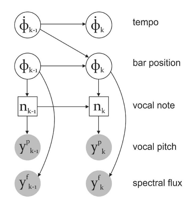
Figure 1: A dynamic Bayesian network for the proposed beat and vocal onset detection model. Circles and squares denote continuous and discrete variables, respectively. Gray nodes and white nodes represent observed and hidden variables, respectively.

In the proposed DBN, an observed sequence of features derived from an audio signal $y_{1:K}=\{y,..,y_{K}\}$ is generated by a sequence of hidden (unknown) variables $x_{1:K}=\{x_{1},...,x_{K}\}$, where K is the length of the sequence (number of audio frames in an audio excerpt). The joint probability distribution of hidden and observed variables factorizes as:

$$P(x_{1:K},y_{1:K})=P(x_{0})\Pi_{k=1}^{K}P(x_{k}|x_{k-1})P(y_{k}|x_{k})$$ (1)

where $P(x_{0})$ is the initial state distribution; $P(x_{k}|x_{k-1})$ is the transition model and $P(y_{k}|x_{k})$ is the observation model.

4.1 Hidden variables

At each audio frame $k$, the hidden variables describe the state of a hypothetical bar pointer $x_{k}=[\dot{\phi_{k}},\phi_{k},n_{k}]$, representing the instantaneous tempo, the bar position and the vocal note respectively.

4.1.1 Tempo state $\dot{\phi}$ and bar position state $\phi$

The bar position $\phi$ points to the current position in the metrical cycle (bar). The instantaneous tempo $\dot{\phi}$ encodes how many bar positions the pointer advances from the current to the next time instant. To assure feasible computational time we relied on the combined bar-tempo efficient state space, presented in [12]. To keep the size of the bar-tempo state space small, we input the ground truth tempo for each recording, allowing a range for $\dot{\phi}$ within $\pm 10$ bpm from it, in order to accommodate gradual tempo changes. This was the minimal margin at which beat tracking accuracy did not degrade substantially. For a study with data with higher stylistic diversity, it would make sense to increase it to at least 20% as it is done in [8, Section 5.2]. This yields around 100-1000 states for the bar positions within a single beat (in the order of $5000$ for 4 beats, and $10000$ for 8-9 beats for the usuls ).

4.1.2 Vocal note state $n$

The vocal note states represent the temporal segments of a sung note. They are a modified version of these suggested in the note transcription model of [14]. We adopted the first two segments: attack region (A), stable pitch region (S). We replaced the silent segment with non-vocal state (N). Because full-fledged note transcription is outside the scope of this work, instead of 3 steps per semitone, we used for simplicity only a single one, which deteriorated just slightly the note onset detection accuracy. Also, to reflect the pitch range in the datasets, on which we evaluate, we set as minimal MIDI note E3 covering almost 3 octaves up to B5 (35 semitones). This totals to 105 note states.

To be able to represent the DBN as an HMM, the bar-tempo efficient state space is combined with the note state space into a joint state space x. The joint state space is a cartesian product of the two state spaces, resulting in up to $10000$$\times 105\approx 1\thinspace$M states.

4.2 Transition model

Due to the conditional dependence relations in Figure 1 the transitional model factorizes as

$$\begin{array}[]{cc}P(x_{k}|x_{k-1})=&P(\dot{\phi}_{k}|\dot{\phi}_{k-1})\thinspace\times\\ P(\phi_{k}|\phi{}_{k-1},\dot{\phi}_{k-1})\thinspace\times&P(n_{k}|n_{k-1},\phi_{k})\end{array}$$ (2)

The tempo transition probability $p(\dot{\phi_{k}}|\dot{\phi}_{k-1})$ and bar position probability $p(\phi_{k}|\phi_{k-1},\dot{\phi}_{k-1})$ are the same as in [12]. Transition from one tempo to another is allowed only at bar positions, at which the beat changes. This is a reasonable assumption for the local tempo deviations in the analyzed datasets, which can be considered to occur relatively beat-wise.

4.2.1 Note transition probability

The probability of advancing to a next note state is based on the transitions of the note-HMM, introduced in [14]. Let us briefly review it: From a given note segment the only possibility is to progress to its following note segment. To ensure continuity each of the self-transition probabilities is rather high, given by constants $c_{A}$, $c_{S}$ and $c_{N}$ for A, S and N segments respectively ($c_{A}$=0.9; $c_{S}$=0.99; $c_{N}=0.9999$). Let $P_{N_{i}A_{j}}$ be the probability of transition from non-vocal state $N_{i}$ after note $i$ to attack state $A_{j}$ of its following note $j$. The authors assume that it depends on the difference between the pitch values of notes $i$ and $j$ and it can be approximated by a normal distribution centered at change of zero ([14], Figure 1.b). This implies that small pitch changes are more likely than larger ones. Now we can formalize their note transition as:

$$p(n_{k}|n_{k-1})=\begin{cases}P_{N_{i}A_{j}},&n_{k-1}=N_{i}\quad n_{k}=A_{j}\\ c_{N},&n_{k-1}=n_{k}=N_{i}\\ 1-c_{A},&n_{k-1=}A_{i}\quad n_{k}=S_{j}\\ c_{A},&n_{k-1}=n_{k}=A_{i}\\ 1-c_{S}&n_{k=1}=S_{i\quad}n_{k}=N_{j}\\ c_{S},&n_{k-1}=n_{k}=S_{i}\\ 0&else\end{cases}$$ (3)

Note that the outbound transitions from all non-vocal states $N_{i}$ should sum to 1, meaning that

$$c_{N}=1-\sum_{i}P_{N_{i}A_{j}}$$ (4)

In this study, we modify $P_{N_{i}A_{j}}$ to allow variation in time, depending on the current bar position $\phi_{k}$.

$$p(n_{k}|n_{k-1,}\phi_{k})=\begin{cases}P_{N_{i}A_{j}}\Theta(\phi_{k}),&n_{k-1}=N_{i},n_{k}=A_{j}\\ c_{N},&n_{k-1}=n_{k}=N_{i}\\ ...\end{cases}$$ (5)

where

$\Theta(\phi_{k}):$

function weighting the contribution of a beat adjacent to current bar position $\phi_{k}$

and

$$c_{N}=1-\Theta(\phi_{k})\sum_{i}P_{N_{i}A_{j}}$$ (6)

The transition probabilities in all the rest of the cases remain the same. We explore two variants of the weighting function $\Theta(\phi_{k}):$

1. Time-window redistribution weighting: Singers often advance or delay slightly note onsets off the location of a beat. The work [15] presented an idea on how to model vocal onsets, time-shifted from a beat, by stochastic distribution. Similarly, we introduce a normal distribution $\mathcal{N}{}_{0,\sigma}$, centered around 0 to re-distribute the importance of a metrical accent (beat) over a time window around it. Let $b_{k}$ be the beat, closest in time to a current bar position $\phi_{k}$. Now:

$$\Theta(\phi_{k})=[\mathcal{N}_{0,\sigma}(d(\phi_{k},b_{k}))]^{w}e(b_{k})$$ (7)

where

$e(b):$

probability of a note onset co-occurring with the $b^{th}$ beat (b $\in$$B$); $B$ is the number of beats in a metrical cycle

$w:$

sensitivity of vocal onset probability to beats

$d(\phi_{k},b_{k}):$

the distance from current bar position $\phi_{k}$ to the position of the closest beat $b_{k}$

Equation 5 means essentially that the original $P_{N_{i}A_{j}}$ is scaled according to how close in time to a beat it is.

2. Simple weighting: We also aim at testing a more conservative hypothesis that it is sufficient to approximate the influence of metrical accents only at the locations of beats. To reflect that, we modify the $P_{N_{i}A_{j}}$ only at bar positions corresponding to beat positions, for which the weighting function is set to the peak of $N_{0,\sigma}$, and to 1 elsewhere.

$$\Theta(\phi_{k})=\begin{cases}[N_{0,\sigma}(0)]^{w}e(b_{k}),&d(\phi_{k},b_{k})=0\\ 1&else\end{cases}$$ (8)

4.3 Observation models

The observation probability $P(y_{k}|x_{k})$ describes the relation between the hidden states and the (observed) audio signal. In this work we make the assumption that the observed vocal pitch and the observed metrical accent are conditionally independent from each other. This assumption may not hold in cases when energy accents of singing voice, which contribute to the total energy of the signal, are correlated to changes in pitch. However, for music with percussive instruments the importance of singing voice accents is diminished to a significant extent by percussive accents. Now we can rewrite Eq. 1 as

$$\begin{array}[]{cc}P(x_{1:K},y_{1:K}^{f},y_{1:K}^{p})=\\[3.0pt] P(x_{0})\Pi_{k=1}^{K}P(x_{k}|x_{k-1})P(y_{k}^{f}|x_{k})P(y_{k}^{p}|x_{k})\end{array}$$ (9)

This means essentially that the observation probability can be represented as the product of the observation probability of a metrical accent $P(y_{k}^{f}|x_{k})$ and the observation probability of vocal pitch $P(y_{k}^{p}|x_{k})$.

4.3.1 Accent observation model

In this paper for $P(y_{k}^{f}|x_{k})$ we train GMMs on the spectral flux-like feature $y^{f}$, extracted from the audio signal using the same parameters as in [12] and [9]. The feature vector $y^{f}$ summarizes the energy changes (accents) that are likely to be related to the onsets of all instruments together. This forms a rhythmic pattern of the accents, characteristic for a given metrical type. The probability of observing an accent thus depends on the position in the rhythmic pattern, $P(y_{k}^{f}|x_{k})=P(y_{k}^{f}|\phi_{k})$.

4.3.2 Pitch observation model

The pitch probability $P(y_{k}^{p}|x_{k})$ reduces to $P(y_{k}^{p}|n_{k})$, because it depends only on the current vocal note state. We adopt the idea proposed in [14] that a note state emits pitch $y^{p}$ according to a normal distribution, centered around its average pitch. The standard deviation of stable states and the one of the onset states are kept the same as in the original model, respectively 0.9 and 5 semitones. The melody contour of singing is extracted in a preprocessing step. We utilized for English pop a method for predominant melody extraction [19]. For Turkish makam, we instead utilized an algorithm, extended from [19] and tailored to Turkish makam [1]. In both algorithms, each audio frame $k$ gets assigned a pitch value and probability of being voiced $v_{k}$ . Based on frames with zero probabilities, one can infer which segments are vocal and which not. Since correct vocal segments is crucial for the sake of this study and the voicing estimation of these melody extraction algorithms are not state of the art, we manually annotated segments with singing voice, and thus assigned $v_{k}=0$ for all frames, annotated as non-vocal.

For each state the observation probability $P(y_{k}^{p}|n_{k})$ of vocal states is normalized to sum to $v_{k}$ (unlike the original model which sums to a global constant v). This leaves the probability for each non-vocal state be $\nicefrac{{1-v_{k}}}{{n}}$.

4.4 Learning model parameters

4.4.1 Accent observation model

We trained the metrical accent probability $P(y_{k}^{f}|\phi_{k})$ separately for each meter type: The Turkish meters are trained on the training subset of the makam dataset (see section 3.1). For each usul (8/8 and 9/8) we trained a rhythmic pattern by fitting a 2-mixture GMM on the extracted feature vector $y^{f}$. Analogously to [12], we pooled the bar positions down to 16 patterns per beat. For English pop we used the 4/4 rhythmic pattern, trained by [11] on ballroom dances. The feature vector is normalized to zero mean, unit variance and taking moving average. Normalization is done per song.

4.4.2 Probability of note onset

The probability of a vocal note onset co-occurring at a given bar position $e(b)$ is obtained from studies on sheet music. Many notes are aligned with a beat in the music score, meaning a higher probability of a note at beats compared to inter-beat bar positions. A separate distribution $e(b)$ is applied for each different metrical cycle. For the Turkish usuls $e(b)$ has been inferred from a recent study [7, Figure 5. a-c]. The authors used a corpus of music scores, on data from the same corpus, from which we derived the Turkish dataset. The patterns reveal that notes are expected to be located with much higher likelihoods on those beats with percussive strokes than on the rest.

In comparison to a classical tradition like makam, in modern pop music the most likely positions of vocal accents in a bar are arguably much more heterogeneous, due to the big diversity of time-deviations from one singing style to another [10]. Due to lack of a distribution pattern $e(b)$, characteristic for English pop, we set it manually with probabilities $(0.8,0.6,0.8,0.6)$ for the 4 beats.

4.5 Inference

We obtain the most optimal state sequence $x_{1:K}$ by decoding with the Viterbi algorithm. A note onset is detected when the state path enters an attack note state after being in non-vocal state.

4.5.1 With manually annotated beats

We explored the option that beats are given as input from a preprocessing step (i.e. when they are manually annotated). In this case, the detection of vocal onsets can be carried out by a reduced model with a single hidden variable: the note state. The observation model is then reduced to the pitch observation probability. The transition model is reduced to a bar-position aware transition probability $a_{ij}(k)=p(n_{k}=j|n_{k-1}=i,\phi_{k})$ (see Eq. 5). To represent the time-dependent self-transition probabilities we utilize time-varying transition matrix. The standard transition probabilities in the Viterbi maximization step are substituted for the bar-position aware transitions $a_{ij}(k)$

$$\delta_{k}(j)=\max_{i\in(j,\thinspace j-1)}\delta_{k-1}(i)\thinspace a_{ij}(k)\thinspace b_{j}(O_{k})$$ (10)

Here $b_{j}(O_{k})$ is the observation probability for state $i$ for feature vector $O_{k}$ and $\delta_{k}(j)$ is the probability for the path with highest probability ending in state $j$ at time $k$ (complying with the notation of [16, III. B]

4.5.2 Full model

In addition to onsets, a beat is detected when the bar position variable hits one of $B$ positions of beats within the metrical cycle.

Note that the size of the state space $x$ poses a memory requirement. A recording of 1 minute has around $10000$ frames at a hopsize of $5.8\thinspace$ms. To use Viterbi thus requires to store in memory pointers to up to $4\thinspace$G states, which amounts to $40\thinspace$G RAM (with uint32 python data type).

5 Experiments

The hopsize of computing the spectral flux feature, which resulted in most optimal beat detection accuracy in [12] is $h_{f}=20\thinspace$ms. In comparison, the hopsize of predominant vocal melody detection is usually of smaller order i.e. $h_{p}=5.8\thinspace$ms (corresponding to 256 frames at sampling rate of 44100). Preliminary experiments showed that extracting pitch with values of $h_{p}$ bigger than this values reasonably deteriorates the vocal onset accuracy. Therefore in this work we use hopsize of $5.8\thinspace$ms for the extraction of both features. The time difference parameter for the spectral flux computation remains unaffected by this change in hopsize, because it can be set separately.

As a baseline we run the algorithm of [14] with the 105 note states, we introduced in Section 4.1.2. The note transition probability is the original as presented in Eq. 3, i.e. not aware of beats. Note that in [14] the authors introduce a post-processing step, in which onsets of consecutive sung notes with same pitch are detected considering their intensity difference. We excluded this step in all system variants presented, because it could not be integrated in the proposed observation model in a trivial way. This means that, essentially, in this paper cases of consecutive same-pitch notes are missed, which decreases inevitably recall, compared to the original algorithm.

meter		beat Fmeas	P	R	Fmeas
aksak	Mauch	-	33.1	31.6	31.6
	Ex-1	-	37.5	38.4	37.2
	Ex-2	86.4	37.8	36.1	36.1
düyek	Mauch	-	42.1	36.9	37.9
	Ex-1	-	44.3	41.0	41.4
	Ex-2	72.9	45.0	39.0	40.3

(a)

meter		beat Fmeas	P	R	Fmeas
4/4	Mauch	-	29.6	38.3	33.2
	Ex-1	-	30.3	42.5	35.1
	Ex-2	94.2	31.6	39.4	34.4
total	Mauch	-	34.8	35.6	35.2
	Ex-1	-	38.3	40.6	39.5
	Ex-2	84.3	38.1	38.2	38.1

(b)

Table 1: Evaluation results for Experiment 1 (shown as Ex-1) and Experiment 2 (shown as Ex-2). Mauch stands for the baseline, following the approach of [14]. P, R and Fmeas denote the precision, recall and f-measure of detected vocal onsets. Results are averaged per meter type.

5.1 Evaluation metrics

5.1.1 Beat detection

Since improvement of the beat detector is outside the scope of this study, we report accuracy of detected beats only in terms of their f-measure. This serves solely the sake of comparison to existing work. The f-measure can take a maximum value of 1, while beats tapped on the off-beat relative to annotations will be assigned an f-measure of 0. We used the default tolerance window of $70\thinspace$ms, also applied in [9].

5.1.2 Vocal onset detection

We measured vocal onset accuracy in terms of precision and recall. Unlike a cappella singing, the exact onset times of singing voice accompanied by instruments, might be much more ambiguous. To accommodate this fact, we adopted the tolerance of $t=50\thinspace$ms, used for vocal onsets in accompanied flamenco singing by [13], which is much bigger than the $t=5\thinspace$ms used by [14] for a cappella. Note that measuring transcription accuracy remains outside the scope of this study.

5.2 Experiment 1: With manually annotated beats

As a precursor to evaluating the full-fledged model, we conducted an experiment with manually annotated beats. This is done to test the general feasibility of the proposed note transition model (presented in 4.2.1), unbiased from errors in the beat detection.

We did apply both the simple and the time-redistribution weighting schemes, presented respectively in Eq. 8 and in Eq. 7. In preliminary experiments we saw that with annotated beats the simple weighting yields much worse onset accuracy than the time-redistributed one. Therefore the results reported are conducted with the latter weighting.

We have tested different pairs of values for $w$ and $\sigma$ from Eq. 5. For Turkish makam the onset detection accuracy peaks at $w=1.2$ and $\sigma=30\thinspace$ms, whereas for the English pop optimal are $w=1.1$ and $\sigma=45\thinspace$ms. Table 1 presents metrics compared to the baseline. Inspection of detections revealed that the metrical-accent aware model could successfully detect certain onsets close to beats, which are omitted by the baseline.

5.3 Experiment 2: Full model

To assure computational efficient decoding, we did an efficient implementation of the joint state space of [12]. To compare to that work, we measured the beat detection with both their original implementation and our proposed one. Expectedly, the average f-measure of the detected beats were the same for each of the three metrical cycle types in the datasets, which can be seen in Table 1. For aksak and düyek usuls, the accuracy is somewhat worse than the results of $91$ and $85.2$ respectively, reported in [9, Table 1.a-c, R=1]. We believe the reason is in the smaller size of our training data. Table 1 evidences also a reasonable improvement of the vocal onset detection accuracy for both music traditions. The results reported are only with the simple weighting scheme for the vocal note onset transition model (the time-redistribution weighting was not implemented in this experiment).

Adding the automatic beat tracking improved the baseline, whereas this was not the case with manual beats for simple weighting. This suggests that the concurrent tracking of beats and vocal onsets is a flexible strategy and can accommodate some vocal onsets, slightly time-shifted from a beat. We observe also that the vocal onset accuracy is on average a bit inferior to that with manual beat annotations (done with the time-redistribution weighting).

For the 4/4 meter, despite the highest beat detection accuracy, the improvement of onset accuracy over the baseline is the least. One reason for that may be that the note probability pattern $e(b)$, used for 4/4 is not well representative for the singing style differences.

A paired t-test between the baseline and each of Ex-1 and Ex-2 resulted in p-values of respectively $0.28$ and $0.31$ on total for all meter types. We expect that statistical significance can be evaluated more accurately with a bigger number of recordings.

6 Conclusions

In this paper we presented a Bayesian approach for tracking vocal onsets of singing voice in polyphonic music recordings. The main contribution is that we integrate in one coherent model two existing probabilistic approaches for different tasks: beat tracking and note transcription. Results confirm that the knowledge of the current position in the metrical cycle can improve the accuracy of vocal note onset detection over different metrical cycle types. The model has a comprehensive set of parameters, whose appropriate tuning allows application to material with different singing style and meter.

In the future the manual adjustment of these parameters could be replaced by learning their values from sufficiently big training data, which was not present for this study. In particular, the lakh-vocal-segments dataset could be easily extended substantially, which we plan to do in the future. Moreover, one could decrease the expected parameter values range, based on learnt values, and thus decrease the size of the state space, which is a current computational limitation. We believe that the proposed model could be applied as well to full-fledged transcription of singing voice.

Acknowledgements

We thank Sebastian Böck for the implementation hints. Ajay Srinivasamurthy is currently with the Idiap Research Institute, Martigny, Switzerland.

This work is partly supported by the European Research Council under the European Union’s Seventh Framework Program, as part of the CompMusic project (ERC grant agreement 267583) and partly by the Spanish Ministry of Economy and Competitiveness, through the ”María de Maeztu” Programme for Centres/Units of Excellence in R&D” (MDM-2015-0502).

References

- [1] Hasan Sercan Atlı, Burak Uyar, Sertan Şentürk, Barış Bozkurt, and Xavier Serra. Audio feature extraction for exploring Turkish makam music. In Proceedings of 3rd International Conference on Audio Technologies for Music and Media (ATMM 2014), pages 142–153, Ankara, Turkey, 2014.
- [2] Emmanouil Benetos, Simon Dixon, Dimitrios Giannoulis, Holger Kirchhoff, and Anssi Klapuri. Automatic music transcription: challenges and future directions. Journal of Intelligent Information Systems, 41(3):407–434, 2013.
- [3] Sungkyun Chang and Kyogu Lee. A pairwise approach to simultaneous onset/offset detection for singing voice using correntropy. In Proceedings of the IEEE International Conference on Acoustics, Speech and Signal Processing (ICASSP), pages 629–633. IEEE, 2014.
- [4] Norberto Degara, Antonio Pena, Matthew EP Davies, and Mark D Plumbley. Note onset detection using rhythmic structure. In Proceedings of the IEEE International Conference on Acoustics, Speech and Signal Processing (ICASSP), pages 5526–5529. IEEE, 2010.
- [5] Masataka Goto. Singing information processing. In 12th International Conference on Signal Processing (ICSP), pages 2431–2438. IEEE, 2014.
- [6] Masataka Goto, Hiroki Hashiguchi, Takuichi Nishimura, and Ryuichi Oka. RWC music database: Popular, classical, and jazz music databases. In Proceedings of the 3rd International Conference on Music Information Retrieval (ISMIR 2002), pages 287–288, 2002.
- [7] Andre Holzapfel. Relation between surface rhythm and rhythmic modes in turkish makam music. Journal of New Music Research, 44(1):25–38, 2015.
- [8] Andre Holzapfel and Thomas Grill. Bayesian meter tracking on learned signal representations. In Proceedings of the 17th International Society for Music Information Retrieval Conference (ISMIR 2016), pages 262–268, 2016.
- [9] Andre Holzapfel, Florian Krebs, and Ajay Srinivasamurthy. Tracking the “odd”: Meter inference in a culturally diverse music corpus. In Proceedings of the 15th International Society for Music Information Retrieval Conference (ISMIR 2014), pages 425–430, Taipei, Taiwan, 2014.
- [10] David Brian Huron. Sweet anticipation: Music and the psychology of expectation. MIT press, 2006.
- [11] Florian Krebs, Sebastian Böck, and Gerhard Widmer. Rhythmic pattern modeling for beat and downbeat tracking in musical audio. In Proceedings of the 14th International Society for Music Information Retrieval Conference (ISMIR 2013), Curitiba, Brazil, 2013.
- [12] Florian Krebs, Sebastian Böck, and Gerhard Widmer. An Efficient State-Space Model for Joint Tempo and Meter Tracking. In Proceedings of the 16th International Society for Music Information Retrieval Conference (ISMIR 2015), pages 72–78, Malaga, Spain, October 2015.
- [13] Nadine Kroher and Emilia Gómez. Automatic transcription of flamenco singing from polyphonic music recordings. IEEE Transactions on Audio, Speech and Language Processing, 24(5):901–913, 2016.
- [14] Matthias Mauch, Chris Cannam, Rachel Bittner, George Fazekas, Justin Salamon, Jiajie Dai, Juan Bello, and Simon Dixon. Computer-aided melody note transcription using the tony software: Accuracy and efficiency. In Proceedings of the First International Conference on Technologies for Music Notation and Representation (TENOR 2015), pages 23–30, 2015.
- [15] Ryo Nishikimi, Eita Nakamura, Katsutoshi Itoyama, and Kazuyoshi Yoshii. Musical note estimation for F0 trajectories of singing voices based on a bayesian semi-beat-synchronous HMM. In Proceedings of the 17th International Society for Music Information Retrieval Conference, (ISMIR 2016), pages 461–467, 2016.
- [16] Lawrence Rabiner. A tutorial on hidden Markov models and selected applications in speech recognition. Proceedings of the IEEE, 77(2):257–286, 1989.
- [17] Colin Raffel. Learning-Based Methods for Comparing Sequences, with Applications to Audio-to-MIDI Alignment and Matching. PhD thesis, Columbia University, 2016.
- [18] Matti Ryynänen. Probabilistic modelling of note events in the transcription of monophonic melodies. Master’s thesis, 2004.
- [19] Justin Salamon and Emilia Gómez. Melody extraction from polyphonic music signals using pitch contour characteristics. IEEE Transactions on Audio, Speech, and Language Processing, 20(6):1759–1770, 2012.
- [20] Nick Whiteley, Ali Taylan Cemgil, and Simon Godsill. Bayesian modelling of temporal structure in musical audio. In Proceedings of the 7th International Society for Music Information Retrieval Conference (ISMIR 2006), pages 29–34, Victoria, Canada, October 2006.