A closure theory for the split energy-helicity cascades in homogeneous isotropic homochiral turbulence

Abstract

We study the energy transfer properties of three dimensional homogeneous and isotropic turbulence where the non-linear transfer is altered in a way that helicity is made sign-definite, say positive. In this framework, known as homochiral turbulence, an adapted eddy-damped quasi-normal Markovian (EDQNM) closure is derived to analyze the dynamics at very large Reynolds numbers, of order $10^{5}$ based on the Taylor scale. In agreement with previous findings, an inverse cascade of energy with a kinetic energy spectrum like $\propto k^{-5/3}$ is found for scales larger than the forcing one. Conjointly, a forward cascade of helicity towards larger wavenumbers is obtained, where the kinetic energy spectrum scales like $\propto k^{-7/3}$. By following the evolution of the closed spectral equations for a very long time and over a huge extensions of scales, we found the developing of a non monotonic shape for the front of the inverse energy flux. The very long time evolution of the kinetic energy and integral scale in both the forced and unforced cases is analyzed also.

I Introduction

Since the discovery that helicity is an inviscid invariant of the three-dimensional Navier-Stokes equations Moffatt (1969), the possibility of inverse cascades in homogeneous isotropic turbulence (HIT) without mirror symmetry has been greatly investigated: indeed, two-dimensional turbulence possesses as well two inviscid invariants, kinetic energy and enstrophy, and in this configuration, energy cascades towards large scales (Boffetta and Ecke, 2012).

In 3D, the first theoretical considerations date back to the study of Brissaud and coworkers (Brissaud et al., 1973) where two different scenarios were proposed: (i) a joint direct cascade of kinetic energy and helicity where $E(k)\sim\epsilon^{2/3}k^{-5/3}$, and $H(k)\sim\epsilon_{H}\epsilon^{-1/3}k^{-5/3}$, where $E$ and $H$ are the kinetic and helical spectra, and $\epsilon$ and $\epsilon_{H}$ the kinetic energy and helicity dissipation rates; (ii) a split cascade with a direct transfer of helicity combined with an inverse cascade of kinetic energy. In fact, the second scenario was proven to be impossible by André and Lesieur (1977) within the eddy-damped quasi-normal Markovian (EDQNM) approximation (Orszag, 1970; Lesieur, 2008; Sagaut and Cambon, 2008). In subsequent papers like Borue and Orszag (1997); Chen et al. (2003) and more recently Briard and Gomez (2017), the joint direct cascade of helicity was observed in HIT without mirror symmetry, with strictly zero inverse energy transfer. This stems from the fact that helicity, the scalar product of velocity and vorticity, is not positive-definite, unlike kinetic energy and enstrophy.

Keeping this later feature in mind, Biferale and coworkers (Biferale et al., 2012, 2013) performed a ”surgery” of the triadic Fourier interactions of turbulence, following the ideas developed by Waleffe (1992), in order to keep only the ones that maintain the helicity sign-definite, yielding to the so-called homochiral turbulence. They consequently recovered the second scenario of Brissaud et al. (1973), namely an inverse cascade of kinetic energy and a forward cascade of helicity, showing that all three dimensional turbulent flows indeed possess a sub-set of Fourier interactions potentially able to sustain an inverse energy cascade. Such a ”surgery” of the Navier-Stokes equations was thoroughly investigated in multiple subsequent works (Sahoo et al., 2015, 2017a, 2017b) so that the details are not recalled here. The main findings are that by forcing at small scales the decimated Navier-Stokes (dNS) equations where helicity is made sign-definite, say positive here, kinetic energy is transferred to smaller wavenumbers with $E(k)\sim\epsilon^{2/3}k^{-5/3}$. By forcing at large scales the dNS equations, a direct helicity cascade with $E(k)\sim\epsilon_{H}^{2/3}k^{-7/3}$ was obtained. It was also notably shown that as soon as helicity is not made strictly sign-definite, by adding helical Fourier modes with the opposite helicity (negative here), the inverse energy cascade vanishes, and that the transition between the upward and forward cascades mechanisms looks singular Sahoo et al. (2015, 2017b). On the other hand, by changing the relative weight of homochiral and heterochiral triads, one is led to a transition from direct to inverse cascade for a finite value of the control parameter Sahoo et al. (2017a), showing that the way Navier Stokes equations transfer energy across scales might be strongly different by changing the involved degrees of freedom.

Strangely enough, inverse cascades with EDQNM were rarely investigated in the past and mainly for two configurations only: the inverse cascade of kinetic energy in 2D turbulence (Pouquet et al., 1975), and the inverse cascade of magnetic helicity in isotropic magnetohydrodynamics turbulence (Pouquet et al., 1976). Consequently, it appears interesting in terms of modelling to check that a sophisticated model such as EDQNM can handle complex and particular configurations when only specific triadic interactions are kept. In the present work, we aim at further studying these features when helicity is made sign-definite by deriving a new EDQNM model. We show for the first time that a split cascade scenario develops and that it can be studied for very large Reynolds numbers and for very long times. In what follows, the adapted EDQNM closure for homochiral turbulence is derived, and then numerical results are presented for cases with and without forcing.

II EDQNM closure for homochiral turbulence

The spectral counterpart of the Navier-Stokes equation for the fluctuating velocity $\hat{u}_{i}$ reads in homogeneous isotropic turbulence

$$\left(\frac{\partial}{\partial t}+\nu k^{2}\right)\hat{u}_{j}(\bm{k})=-\mathrm{i}P_{jmn}(\bm{k})\,\int_{\bm{k}=\bm{p}+\bm{q}}u_{m}(\bm{p})u_{n}(\bm{q})\mathrm{d}^{3}\bm{p},$$ (1)

where $\nu$ is the kinematic viscosity, $\mathrm{i}^{2}=-1$, the operator $2P_{jmn}=k_{m}P_{jn}+k_{n}P_{jm}$, with the projector $P_{jn}=\delta_{jn}-\alpha_{j}\alpha_{n}$ and $\alpha_{j}=k_{j}/k$, $k$ and $\bm{k}$ are respectively the wavenumber and wavevector, and $\hat{(\cdot)}$ denotes the Fourier transform. In isotropic turbulence without reflexion symmetry, the spectral second-order velocity-velocity correlation $\hat{R}_{ij}(\bm{k},t)=\langle\hat{u}_{i}^{*}(\bm{k},t)\hat{u}_{j}(\bm{k},t)\rangle$, where $(\cdot)^{*}$ denotes the complex conjugate and $\langle.\rangle$ an ensemble average, can be decomposed as

$$\hat{R}_{ij}(\bm{k},t)=\mathcal{E}(\bm{k},t)P_{ij}(\bm{k})+\mathrm{i}\epsilon_{ijk}\alpha_{k}\frac{\mathcal{H}(\bm{k},t)}{k},$$ (2)

with $\epsilon_{ijk}$ the Levi-Civita permutation tensor, and where $\mathcal{E}$ and $\mathcal{H}$ are respectively the kinetic energy and kinetic helicity densities. Such a decomposition involving the kinetic energy density $\mathcal{E}$ and helical density $\mathcal{H}$ was previously used in Cambon and Jacquin (1989); Borue and Orszag (1997); Chen et al. (2003). More recently Briard and Gomez (2017), this decomposition was applied to investigate with EDQNM the large Reynolds numbers dynamics of the kinetic energy and helical spectra defined as

$$E(k,t)=\int_{S_{k}}\mathcal{E}(\bm{k},t)\mathrm{d}^{2}\bm{k},\qquad H(k,t)=\int_{S_{k}}\mathcal{H}(\bm{k},t)\mathrm{d}^{2}\bm{k},$$ (3)

where $S_{k}$ is a sphere of radius $k$. The total helicity, which is the scalar product of velocity and vorticity, is then obtained by $\langle\bm{u}.\bm{\omega}\rangle/2=\int_{0}^{\infty}H(k,t)\mathrm{d}k$. In what follows, we analyze within an adapted EDQNM approximation at large Reynolds numbers, the configuration proposed in Biferale et al. (2012, 2013), namely the homochiral decimated Navier-Stokes.

To select only helical modes of identical sign the classical Lin equation for $E(k,t)$ (von Kármán and Lin, 1949) and its non-linear transfer of HIT cannot be used anymore. One needs a new closure, adapted to homochiral turbulence where helicity is made sign-definite. First, the spectral fluctuating velocity is decomposed in positive and negative modes using the helical decomposition (Cambon and Jacquin, 1989; Waleffe, 1992; Sagaut and Cambon, 2008) so that

$$\hat{\bm{u}}(\bm{k},t)=u_{+}(\bm{k},t)\bm{N}(\bm{k})+u_{-}(\bm{k},t)\bm{N}^{*}(\bm{k}),$$ (4)

where $\bm{N}$ are the helical modes, which verify $\bm{N}^{*}(\bm{k})=\bm{N}(-\bm{k})$, $\bm{N}.\bm{N}=0$, $\bm{N}.\bm{N}^{*}=2$, and $\mathrm{i}\bm{k}\times\bm{N}=k\bm{N}$, so that the spectral fluctuating vorticity reads

$$\hat{\bm{\omega}}(\bm{k},t)=k\Big{[}u_{+}(\bm{k},t)\bm{N}(\bm{k},t)-u_{-}(\bm{k},t)\bm{N}^{*}(\bm{k},t)\Big{]}.$$ (5)

Considering only the positive helical modes we get for the kinetic energy spectrum:

$$E_{+}(k,t)=\int_{S_{k}}\mathcal{E}_{+}(\bm{k},t)\mathrm{d}^{2}\bm{k}=\int_{S_{k}}\langle u_{+}^{*}(\bm{k},t)u_{+}(\bm{k},t)\rangle\,\mathrm{d}^{2}\bm{k},$$ (6)

and the helical spectrum is thus simply given by $H_{+}(k,t)=kE_{+}(k,t)$. The evolution equation of $u_{+}$ is obtained by contracting (1) with $N_{i}^{*}/2$ which gives

$$\left(\frac{\partial}{\partial t}+\nu k^{2}\right)u_{+}(\bm{k},t)=-\frac{1}{2}\mathrm{i}\Big{(}k_{i}N_{j}^{*}(\bm{k})+k_{j}N_{i}^{*}(\bm{k})\Big{)}\int_{\bm{k}=\bm{p}+\bm{q}}u_{+}(\bm{p})u_{+}(\bm{q})N_{i}(\bm{p})N_{j}(\bm{q})\mathrm{d}^{3}\bm{p}$$ (7)

The evolution equation of the kinetic energy density $\mathcal{E}_{+}$ is then

$$\left(\frac{\partial}{\partial t}+2\nu k^{2}\right)\mathcal{E}_{+}(\bm{k},t)=T_{+}(\bm{k},t).$$ (8)

It is very important to stress that the non-linear terms of the Navier-Stokes equations conserve both energy and helicity triad-by-triad, and therefore the same is true for the dNS. In other words, the non-linear transfer $T_{+}$ is conservative, takes into account triadic interactions of positive helical modes, and reads after some algebra

$$T_{+}(\bm{k},t)=\int\Re\Big{[}\Big{(}k_{i}N_{j}^{*}(\bm{k})+k_{j}N_{i}^{*}(\bm{k})\Big{)}S_{+}(\bm{k},\bm{p},t)N_{i}(\bm{p})N_{j}(\bm{q})\Big{]}\mathrm{d}^{3}\bm{k},$$ (9)

where $S_{+}$ is the spectral triple velocity correlation

$$S_{+}(\bm{k},\bm{p},t)\delta(\bm{k}+\bm{p}+\bm{q})=\mathrm{i}\langle u_{+}(\bm{k},t)u_{+}(\bm{p},t)u_{+}(\bm{q},t)\rangle.$$ (10)

Then, after some technical manipulations typical of the EDQNM approximation (Orszag, 1970; Lesieur, 2008), one obtains the decimated Lin equation of the (positive) kinetic energy spectrum, namely

$$\left(\frac{\partial}{\partial t}+2\nu k^{2}\right)E_{+}(k,t)=S_{+}^{E}(k,t),$$ (11)

where the spherically-averaged non-linear transfer is

$$S_{+}^{E}(k,t) =\int_{S_{k}}T_{+}(\bm{k},t)\mathrm{d}^{2}\bm{k}=16\pi^{2}\int_{\Delta_{k}}k^{2}pq\theta_{kpq}(1+z)\mathcal{E}_{+}^{\prime\prime}\Bigg{[}p\mathcal{E}_{+}(y-z)(y+z-2x)$$

$$+(1-x-2yz)\Big{(}k(1+y)\mathcal{E}_{+}^{\prime}-p(1+x)\mathcal{E}_{+}\Big{)}\Bigg{]}\mathrm{d}p\mathrm{d}q,$$ (12)

with $\Delta_{k}$ the domain where $k$, $p$ and $q$ are the lengths of the sides of the triangle formed by the triad $\bm{k}+\bm{p}+\bm{q}=\bm{0}$, and where $x$, $y$ and $z$ are the cosines of the angles formed by $\bm{p}$ and $\bm{q}$, $\bm{q}$ and $\bm{k}$, and $\bm{k}$ and $\bm{p}$ respectively. For the sake of clarity $\mathcal{E}_{+}=E_{+}(k,t)/4\pi k^{2}$, $\mathcal{E}_{+}^{\prime}=E_{+}(p,t)/4\pi p^{2}$, and $\mathcal{E}_{+}^{\prime\prime}=E_{+}(q,t)/4\pi q^{2}$. $\theta_{kpq}$ is the characteristic time of the triple correlations where the eddy-damping term is given by $A_{1}\sqrt{\int_{0}^{k}u^{2}E_{+}(u,t)\mathrm{d}u}$. Here we will start by taking $A_{1}=0.355$ for consistency with previous studies (Pouquet et al., 1976; Lesieur and Ossia, 2000; Briard et al., 2015; Briard and Gomez, 2017), the impact of changing $A_{1}$ is discussed later on. The previous equations of the EDQNM closure for the sign-definite helicity originating from the decimated Navier-Stokes equation are the main theoretical contributions of this work.

For consistency and clarity, it is recalled that in isotropic helical turbulence (without decimation), the kinetic energy spectrum evolves according to $(\partial_{t}+2\nu k^{2})E=S_{E}$, where $S_{E}$ is the usual isotropic spherically-averaged non-linear transfer, namely

$$S_{E}(k,t)=16\pi^{2}\int_{\Delta_{k}}\theta_{kpq}k^{2}p^{2}q(xy+z^{3})\mathcal{E}^{{}^{\prime\prime}}(\mathcal{E}^{{}^{\prime}}-\mathcal{E})\mathrm{d}p\mathrm{d}q,$$ (13)

where $\mathcal{E}=E(k,t)/4\pi k^{2}$, $\mathcal{E}^{\prime}=E(p,t)/4\pi p^{2}$, and $\mathcal{E}^{\prime\prime}=E(q,t)/4\pi q^{2}$. The eddy-damping term is given by the complete energy spectrum $E$, unlike in the decimated version where it is given by $E_{+}$. The expression (12) is more complicated than (13) in the sense that it is less compact and symmetric: this is due to the further contraction with the helical modes to select only specific triadic interactions.

In what follows, we wish to recover two features of homochiral turbulence: (i) the direct helicity cascade of Biferale et al. (2013) where the kinetic energy spectrum scales as $E_{+}(k)\sim{\epsilon_{H}}^{2/3}k^{-7/3}$ and (ii) the inverse cascade of energy in $E_{+}(k)\sim\epsilon^{2/3}k^{-5/3}$. For the EDQNM simulations, the wavenumber space is discretized using a logarithmic mesh $k_{i+1}=rk_{i}$ for $i=1,\ldots,n$, where $n$ is the total number of modes and $r=10^{1/f}$, $f=15$ being the number of points per decade. It has been checked that increasing $f$, for instance up to $f=20$, does not modify the slopes of the spectra, nor the asymptotic values of the integrated quantities (like kinetic energy) more than $1\%$. This mesh spans from $k_{\text{min}}=10^{-6}k_{L}$ to $k_{\text{max}}=10k_{\eta}$, where $k_{L}$ is the integral wavenumber and $k_{\eta}=(\epsilon/\nu^{3})^{1/4}$ the Kolmogorov wavenumber. The initial kinetic energy spectrum is given by $E_{+}(k)\sim k^{\sigma}\exp(-k^{2})$, where the infrared slope is $\sigma=2$, corresponding to Saffman turbulence. Simulations not presented here revealed that the results of this work are independent of the infrared slope, in particular the findings are the same for Batchelor turbulence ($\sigma=4$). The initial $E_{+}$ is normalized so that $\langle u_{+}^{2}\rangle=\int_{0}^{\infty}E_{+}(k)\mathrm{d}k$ is unit at $t=0$.

III Results at large Reynolds numbers

First, homogeneous homochiral turbulence without any forcing is considered. The $k^{-7/3}$ scaling is recovered in figure 1a at large Reynolds numbers, which corresponds to the forward helicity cascade (Brissaud et al., 1973): this inertial $k^{-7/3}$ range grows with time and spans more than 4 decades at the largest Reynolds number. The noteworthy feature is that even without forcing, if large Reynolds numbers are reached, strong inverse transfers mechanisms occur since the peak of $E_{+}$, given at the integral wavenumber $k_{L}$, increases with time, unlike in fully isotropic decaying turbulence. A further evidence for intense inverse non-local transfers is that, even though the infrared scaling of the kinetic energy spectrum is initially $E_{+}(k<k_{L})\sim k^{2}$, it rapidly becomes $E_{+}(k<k_{L})\sim k^{4}$, which is a signature of strong back transfers (Eyink and Thomson, 2000; Lesieur and Ossia, 2000; Meldi and Sagaut, 2012; Briard et al., 2015). It follows from $E_{+}(k)\sim k^{-7/3}$ that the helical spectrum scales in $H_{+}(k)=kE_{+}(k)\sim k^{-4/3}$.

(a)

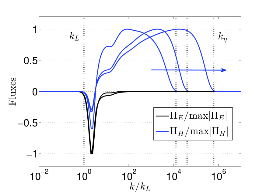
(b)

Figure 1: Time evolution of the kinetic energy spectrum and of the kinetic and helical fluxes for Saffman turbulence ($\sigma=2$): the integral and Kolmogorov wavenumbers $k_{L}$ and $k_{\eta}$ are displayed as vertical dashed lines. (a) $E_{+}(k,t)$ for various times $t=0$, $t=0.1\tau_{0}$, $t=0.5\tau_{0}$ and $t=10^{n}\tau_{0}$ for $n\in[1;6]$, where $\tau_{0}$ is the eddy turnover time: $k_{L}$ and $k_{\eta}$ correspond to the last time (thick spectrum) where $Re_{\lambda}(t=10^{6}\tau_{0})=10^{6}$. (b) Kinetic (black) and helical (blue) fluxes $\Pi_{E}$ and $\Pi_{H}$ for various times $t/\tau_{0}=[10;10^{2};10^{4}]$. For better readability, fluxes are normalized by their maximum value and presented as functions of $k/k_{L}$.

In addition, one can remark from figure 1a that the peak of the kinetic energy spectrum $E_{+}^{\rm peak}$ seems to evolve as $k^{-1}$ with time. This has nothing to do with inertial range scaling considerations, since the inertial range scaling clearly remains $k^{-7/3}$. This can be briefly justified as follows. Since we have mainly a direct helicity cascade, one can roughly assumes that $\epsilon\simeq 0$, consistently with arguments given in Brissaud et al. (1973). Thus, it follows that the kinetic energy $\langle u_{+}^{2}\rangle$, whose evolution is given by $\partial_{t}\langle u_{+}^{2}\rangle=-\epsilon\simeq 0$, remains constant, which is well verified numerically (see later figure 3b). Then, using the definition of the kinetic energy, one can reasonably assume that it is mainly given by the integral scale:

$$\langle u_{+}^{2}\rangle=\int_{0}^{\infty}E_{+}(k,t)\mathrm{d}k\simeq\int_{0}^{k_{L}}E_{+}^{\rm peak}(t)\mathrm{d}k=k_{L}E_{+}^{\rm peak}(t).$$ (14)

The kinetic energy being constant, one obtains that the time evolution of the kinetic energy spectrum peak is given by $E_{+}^{\rm peak}(t)\sim{k_{L}}^{-1}(t)$. Note that for dimensional reasons the integral scale evolves like $L\sim t$ in the unforced case. It will be shown later for the forced case that the time evolution of $\langle u_{+}^{2}\rangle$ and $L$ are quite different. In figure 1b we show the evolution of the two fluxes, $\Pi_{E}$ and $\Pi_{H}$, where $\Pi_{E}(k)=-\int_{0}^{k}S_{+}^{E}(x)\mathrm{d}x$ and $\Pi_{H}(k)=-\int_{0}^{k}xS_{+}^{E}(x)\mathrm{d}x$. As said earlier, both energy and helical transfers with homochiral triadic interactions are conservative: indeed, one has $\Pi_{E}(k\to\infty)=\Pi_{H}(k\to\infty)=0$. Furthermore, there is a direct cascade of helicity since $\Pi_{H}$ is mostly positive in the inertial range and spans more and more decades with time, which is consistent with the $k^{-7/3}$ scaling of $E_{+}$ of figure 1a. In addition, figure 1b illustrates that there is an inverse cascade occurring on a small range around $k_{L}$ for $E_{+}$.

To increase the scaling region of the inverse cascade, we add to the decimated Lin equation (11) a forcing term $F(k)$, to have the possibility to study the split cascade scenario with a well developed inverse energy transfer for asymptotically long times. The forcing term is given by

$$F(k)=C_{1}\exp\ \left(-\frac{1}{(C_{2})^{2}}\left[\ln\left(\frac{k}{k_{f}}\right)\right]^{2}\right),$$ (15)

with $C_{1}$ so that one has $\int_{0}^{\infty}F(k)\mathrm{d}k=1$, $C_{2}=0.1$ and $k_{f}=1$ as proposed in Briard and Gomez (2017). We double checked that the following numerical results are independent of the forcing term by studying also the case with $F(k)\sim k^{4}\exp(-2k^{2})$ (not shown). The time evolution of the kinetic energy spectrum is shown in figure 2a, where the forcing term $F$ is in grey. It is clear that the system develops a split cascade on both sides of the forcing term. Indeed, as time increases, a $k^{-5/3}$ range grows at large scales, similar to the one obtained in Biferale et al. (2012), which is a strong evidence for the inverse cascade of kinetic energy. Whereas for wavenumbers larger than $k_{f}$, the $k^{-7/3}$ range is preserved, as in figure 1a without forcing. It is important to stress that this is the first time where the split energy-helicity simultaneous cascade is observed: this is notably due to the fact that by using EDQNM we can push the resolution on both sides to very large values. It is reasonable to conclude from figure 2a that the non-linear transfers which are at the origin of the inverse cascade are dominantly local in homochiral turbulence: indeed, because of the logarithmic discretization of the wavenumber space, elongated triads corresponding to non-local transfers cannot be taken into account with EDQNM (Lesieur, 2008). This statement does not mean that there are no non-local interactions: indeed, it has been argued that some inverse non-local transfers are responsible for the change of the infrared slope of $E_{+}$ from $k^{2}$ to $k^{4}$ in figure 1a (Métais and Lesieur, 1986).

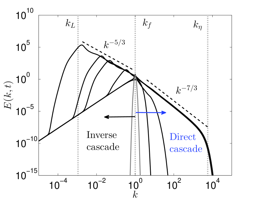
(a)

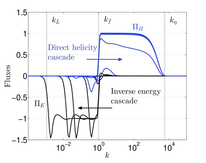
(b)

Figure 2: Time evolution of the kinetic energy spectrum, kinetic and helical fluxes for Saffman turbulence ($\sigma=2$), from $t=0$ to $t=500\tau_{0}$, where the curves are sampled at $t/\tau_{0}=0;1;10;50;100;500$. The integral, forcing, and Kolmogorov wavenumbers $k_{L}$, $k_{f}$, and $k_{\eta}$ are displayed as vertical dashed lines at $Re_{\lambda}(t=500\tau_{0})=3.10^{5}$. (a) $E_{+}(k,t)$ with the forcing term $F(k)$ (grey) defined in (15). (b) Kinetic (black) and helical (blue) fluxes $\Pi_{E}$ and $\Pi_{H}$.

In figure 2b the kinetic and helical fluxes $\Pi_{E}$ and $\Pi_{H}$ are presented. For $k>k_{f}$, at scales smaller than the forcing one, the helical flux is positive, indicating a direct cascade of helicity. For $k<k_{f}$, the helical flux is zero and the kinetic one $\Pi_{E}$ is negative, showing a stable inverse cascade of energy for scales larger than the forcing one. Note that the shape of $\Pi_{E}$ is qualitatively in agreement with the one of Sahoo et al. (2017a) (figure 3 therein, curve marked with squares). Here we show for the first time in a clean way that the inverse transfer has a non trivial wavy shape around the front. The numerical evidence for the split energy cascade in figure 2b further justifies that for $k<k_{f}$ the kinetic energy depends only $\epsilon$ (since $\Pi_{H}$ is almost zero), and that $E_{+}$ and $H_{+}$ only depend on $\epsilon_{H}$ for $k>k_{f}$ (since $\Pi_{E}$ is almost zero). Compensated kinetic energy spectra are presented in figure 3a in the direct and inverse cascades. A reasonable plateau is obtained in both cases spanning two decades. In the inverse cascade, $E_{+}(k)k^{5/3}\epsilon^{-2/3}$ settles around $3.35$, and $E_{+}(k)k^{7/3}{\epsilon_{H}}^{-2/3}$ around $2.7$ in the direct cascade. Both constants are larger than the Kolmogorov one in HIT. For the constant of the inverse cascade, this is somehow consistent with constants of inverse energy cascades found in two-dimensional turbulence which are roughly between 6 and 10 (Kraichnan, 1971; Pouquet et al., 1975; Frisch and Sulem, 1984). Note that the values of the present constants could be modified by changing the eddy-damping parameter $A_{1}$, which is here chosen to be $0.355$ for consistency with previous EDQNM simulations in isotropic and skew-isotropic homogeneous turbulence (Briard et al., 2015; Briard and Gomez, 2017). More specifically, the plateau $E_{+}(k)k^{5/3}\epsilon^{-2/3}$ for the inverse cascade increases with larger eddy-damping constants, namely from $2.3$ to $4.2$, for $A_{1}$ varying from $0.2$ to $0.49$ (this latter value for $A_{1}$ was used in Bos et al. (2012)). The value $4.2$ for the plateau of the inverse cascade is very close to what is obtained in Biferale et al. (2012). To obtain a plateau for $E_{+}(k)k^{5/3}\epsilon^{-2/3}$ around 6 as in 2D turbulence, one would need to go up to $A_{1}=0.8$.

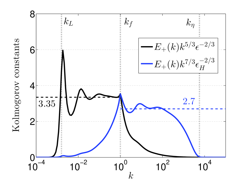
(a)

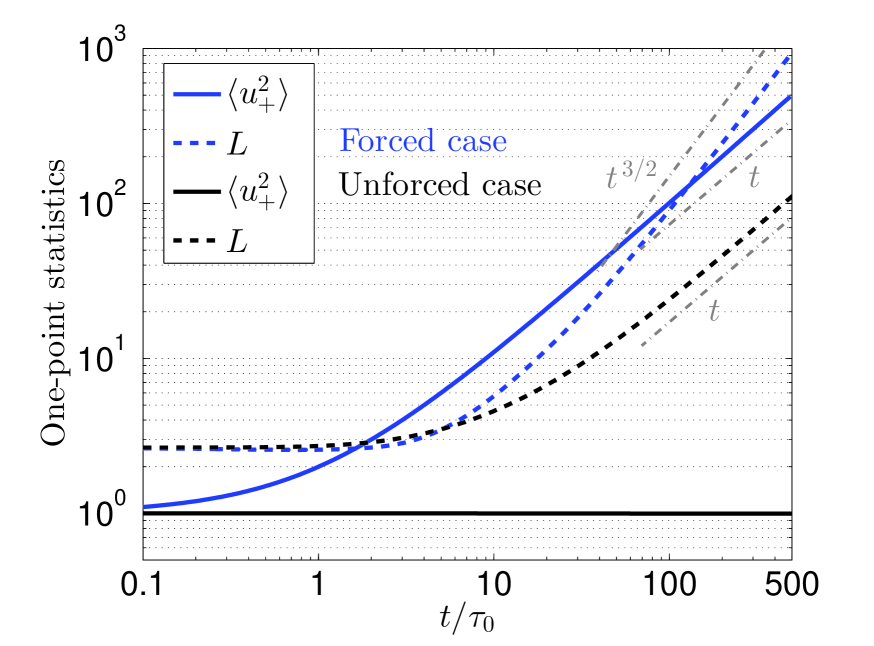
(b)

Figure 3: (a) Compensated kinetic energy spectra in the inverse (black) and direct (blue) cascades. The integral, forcing, and Kolmogorov wavenumbers $k_{L}$, $k_{f}$, and $k_{\eta}$ are displayed as vertical dashed lines at $Re_{\lambda}(t=500\tau_{0})=3.10^{5}$. (b) Time evolution of the kinetic energy $\langle u_{+}^{2}\rangle$ ($-$) and integral scale $L$ ($--$) for $\sigma=2$, for the forced (blue) and unforced (black) cases. The grey $-\cdot$ curves indicate the power laws $t$ and $t^{3/2}$.

Finally, some one-point statistics are presented in figure 3b, namely the kinetic energy $\langle u_{+}^{2}\rangle$ and the integral scale $L=1/k_{L}=3\pi/\langle u_{+}^{2}\rangle\int_{0}^{\infty}(E_{+}(k)/k)\mathrm{d}k$ for both the forced and unforced cases. For the unforced case, the constancy of $\langle u_{+}^{2}\rangle$ and $L\sim t$, discussed earlier, are recovered. For the forced configuration, the kinetic energy is expected to grow as $\langle u_{+}^{2}\rangle\sim\epsilon t$ (Pouquet et al., 1975). The linear dependence with time is recovered in figure 3b. Then, it follows from dimensional analysis $L\sim K^{3/2}/\epsilon$ that the integral scale should evolve like $t^{3/2}$, which is also assessed in figure 3b.

IV Conclusions

In conclusion, we addressed a particular kind of helical turbulence, where only specific triadic interactions are kept, so that the helicity is made sign-definite. In this particular homochiral framework, the 3D turbulence possesses two sign-definite inviscid invariants, namely kinetic energy and helicity, like 2D turbulence with kinetic energy and enstrophy. The main objective of this study was to show that a spectral closure method, such as EDQNM, could recover the main findings of Biferale et al. (2012, 2013). To do so, an adapted EDQNM approximation was derived, taking into account only the particular interactions that make helicity sign-definite (positive here). The direct helicity cascade, where $E_{+}(k)\sim{\epsilon_{H}}^{2/3}k^{-7/3}$, is first obtained in unforced homochiral turbulence, where the kinetic energy flux $\epsilon\simeq 0$. In such a configuration, the kinetic energy $\langle u_{+}^{2}\rangle$ remains constant and the peak of $E_{+}$ evolves in ${k_{L}}^{-1}$ with time. When a forcing term is added, in addition to the helicity forward cascade, an inverse energy cascade develops toward smaller wavenumbers, where the helicity flux $\epsilon_{H}\simeq 0$. In this regime of forced homochiral turbulence, the kinetic energy evolves linearly with time $\langle u_{+}^{2}\rangle\sim\epsilon t$, and the integral scale like $L\sim t^{3/2}$.

Our work shows for the first time the possibility to have a stable split cascade in three dimensional turbulence under strong restriction of the helical interactions. It remains to be understood how much this phenomenology might be indeed observed in more realistic flow configurations, as in the presence of strong rotation or confinement, where also a transition from direct to inverse energy cascade is observed (Mininni and Pouquet, 2009; Celani et al., 2010; Xia et al., 2011; Godeferd and Moisy, 2015; Biferale et al., 2016). It is also interesting to study the inverse cascade regime in the presence of a large scale drag, in order to allow for the formation of a large scale stationary condensate (Chertkov et al., 2007). At difference from the two dimensional case, the condensate will necessarily have strong helical properties and be close to an ABC quasi-stationary solution of the three dimensional Navier-Stokes equations (Dombre et al., 1986; Moffatt, 2014; Sahoo and Biferale, 2015). Work in this direction will be reported elsewhere. Finally, it is important to stress that similar EDQNM studies can be extended to helical MHD (Linkmann et al., 2017).

The research leading to these results has received funding from the European Union’s Seventh Framework Programme (FP7/2007-2013) under grant agreement No. 339032.

References

- Moffatt (1969) H. K. Moffatt, “The degree of knottedness of tangled vortex lines,” Journal of Fluid Mechanics 35, 117–129 (1969).
- Boffetta and Ecke (2012) G. Boffetta and R. E. Ecke, “Two-dimensional turbulence,” Annual Review of Fluid Mechanics 44, 427–451 (2012).
- Brissaud et al. (1973) A. Brissaud, U. Frisch, J. Leorat, M. Lesieur, and A. Mazure, “Helicity cascades in fully developed isotropic turbulence,” The Physics of Fluids 16, 1366–1367 (1973).
- André and Lesieur (1977) J. C. André and M. Lesieur, “Influence of helicity on the evolution of isotropic turbulence at high reynolds number,” Journal of Fluid Mechanics 81, 187–207 (1977).
- Orszag (1970) S. A. Orszag, “Analytical theories of turbulence,” Journal of Fluid Mechanics 41, 363–386 (1970).
- Lesieur (2008) M. Lesieur, Turbulence in fluids (Springer, 4th Edition, Dordrecht, 2008).
- Sagaut and Cambon (2008) P. Sagaut and C. Cambon, Homogeneous Turbulence Dynamics (Cambridge University Press, 2008).
- Borue and Orszag (1997) V. Borue and S.A. Orszag, “Spectra in helical three-dimensional homogeneous isotropic turbulence,” Physical Review E 55, 7005–7009 (1997).
- Chen et al. (2003) Q. Chen, S. Chen, and G. L. Eyink, “The joint cascade of energy and helicity in three-dimensional turbulence,” Physics of Fluids 15, 361 (2003).
- Briard and Gomez (2017) A. Briard and T. Gomez, “Dynamics of helicity in homogeneous skew-isotropic turbulence,” Journal of Fluid Mechanics 821, 539–581 (2017).
- Biferale et al. (2012) L. Biferale, S. Musacchio, and F. Toschi, “Inverse energy cascade in three-dimensional isotropic turbulence,” Physical Review Letters 108, 164501 (2012).
- Biferale et al. (2013) L. Biferale, S. Musacchio, and F. Toschi, “Split energy–helicity cascades in three-dimensional homogeneous and isotropic turbulence,” Journal of Fluid Mechanics 730, 309–327 (2013).
- Waleffe (1992) F. Waleffe, “The nature of triad interactions in homogeneous turbulence,” Physics of Fluids 4, 350–363 (1992).
- Sahoo et al. (2015) G. Sahoo, F. Bonaccorso, and L. Biferale, “Role of helicity for large- and small-scale turbulent fluctuations,” Physical Review E 92, 051002(R) (2015).
- Sahoo et al. (2017a) G. Sahoo, A. Alexakis, and L. Biferale, “Discontinuous transition from direct to inverse cascade in three-dimensional turbulence,” Physical Review Letters 118, 164501 (2017a).
- Sahoo et al. (2017b) G. Sahoo, M. De Pietro, and L. Biferale, “Helicity statistics in homogeneous and isotropic turbulence and turbulence models,” Physical Review Fluids 2, 024601 (2017b).
- Pouquet et al. (1975) A. Pouquet, M. Lesieur, J. C. André, and C. Basdevant, “Evolution of high reynolds number two-dimensional turbulence,” Journal of Fluid Mechanics 72, 305–319 (1975).
- Pouquet et al. (1976) A. Pouquet, U. Frisch, and J.-L. Léorat, “Strong mhd helical turbulence and the nonlinear dynamo effect,” Journal of Fluid Mechanics 77, 321–354 (1976).
- Cambon and Jacquin (1989) C. Cambon and L. Jacquin, “Spectral approach to non-isotropic turbulence subjected to rotation,” Journal of Fluid Mechanics 202, 295–317 (1989).
- von Kármán and Lin (1949) T. von Kármán and C. C. Lin, “On the concept of similiarity in the theory of isotropic turbulence,” Rev. Mod. Phys. 21, 516–519 (1949).
- Lesieur and Ossia (2000) M. Lesieur and S. Ossia, “3d isotropic turbulence at very high reynolds numbers: Edqnm study,” Journal of Turbulence 1 (2000).
- Briard et al. (2015) A. Briard, T. Gomez, P. Sagaut, and S. Memari, “Passive scalar decay laws in isotropic turbulence: Prandtl effects,” Journal of Fluid Mechanics 784, 274–303 (2015).
- Eyink and Thomson (2000) G. L. Eyink and D. J. Thomson, “Free decay of turbulence and breakdown of self-similarity,” Physics of Fluids 12, 477–479 (2000).
- Meldi and Sagaut (2012) M. Meldi and P. Sagaut, “On non-self-similar regimes in homogeneous isotropic turbulence decay,” Journal of Fluid Mechanics 711, 364–393 (2012).
- Métais and Lesieur (1986) O. Métais and M. Lesieur, “Statistical predictability of decaying turbulence,” Journal of the atmospheric sciences 43, 857–870 (1986).
- Kraichnan (1971) R. H. Kraichnan, “Inertial-range transfer in two- and three-dimensional turbulence,” Journal of Fluid Mechanics 47, 525–535 (1971).
- Frisch and Sulem (1984) U. Frisch and P. L. Sulem, “Numerical simulation of the inverse cascade in two-dimensional turbulence,” Physics of Fluids 27, 1921–1923 (1984).
- Bos et al. (2012) W. J. T. Bos, L. Chevillard, J. F. Scott, and R. Rubinstein, “Reynolds number effect on the velocity increment skewness in isotropic turbulence,” Physics of Fluids 24, 015108 (2012).
- Mininni and Pouquet (2009) P.D. Mininni and A. Pouquet, “Helicity cascades in rotating turbulence,” Physical Review E 79, 026304 (2009).
- Celani et al. (2010) A. Celani, S. Musacchio, and D. Vincenzi, “Turbulence in more than two and less than three dimensions,” Physical Review Letters 104, 184506 (2010).
- Xia et al. (2011) H. Xia, D. Byrne, G. Falkovich, and M. Shats, “Upscale energy transfer in thick turbulent fluid layers,” Nature Physics 7, 321 (2011).
- Godeferd and Moisy (2015) F. S. Godeferd and F. Moisy, “Structure and dynamics of rotating turbulence: A review of recent experimental and numerical results,” Appl. Mech. Rev. 67, 030802 (2015).
- Biferale et al. (2016) L. Biferale, F. Bonaccorso, I. M. Mazzitelli, M. A. T. van Hinsberg, A. S. Lanotte, S. Musacchio, P. Perlekar, and F. Toschi, “Coherent structures and extreme events in rotating multiphase turbulent flows,” Phys. Rev. X 6, 041036 (2016).
- Chertkov et al. (2007) M. Chertkov, C. Connaughton, I. Kolokolov, and V. Lebedev, “Dynamics of energy condensation in two-dimensional turbulence,” Physical Review Letters 99, 084501 (2007).
- Dombre et al. (1986) T. Dombre, U. Frisch, J. M. Greene, M. Hénon, A. Mehr, and A. M. Soward, “Chaotic streamlines in the abc flows,” Journal of Fluid Mechanics 167, 353–391 (1986).
- Moffatt (2014) H. K. Moffatt, “Helicity and singular structures in fluid dynamics,” Proceedings of the National Academy of Sciences 111, 3663–3670 (2014).
- Sahoo and Biferale (2015) G. Sahoo and L. Biferale, “Disentangling the triadic interactions in navier-stokes equations,” The European Physical Journal E 38, 114 (2015).
- Linkmann et al. (2017) M. Linkmann, G. Sahoo, M. McKay, A. Berera, and L. Biferale, “Effects of magnetic and kinetic helicities on the growth of magnetic fields in laminar and turbulent flows by helical fourier decomposition,” The Astrophysical Journal 836, 26 (2017).