Optimal Beamforming for Gaussian MIMO Wiretap Channels with Two Transmit Antennas

Abstract

A Gaussian multiple-input multiple-output wiretap channel in which the eavesdropper and legitimate receiver are equipped with arbitrary numbers of antennas and the transmitter has two antennas is studied in this paper. Under an average power constraint, the optimal input covariance to obtain the secrecy capacity of this channel is unknown, in general. In this paper, the input covariance matrix required to achieve the capacity is determined. It is shown that the secrecy capacity of this channel can be achieved by linear precoding. The optimal precoding and power allocation schemes that maximize the achievable secrecy rate, and thus achieve the capacity, are developed subsequently. The secrecy capacity is then compared with the achievable secrecy rate of generalized singular value decomposition (GSVD)-based precoding, which is the best previously proposed technique for this problem. Numerical results demonstrate that substantial gain can be obtained in secrecy rate between the proposed and GSVD-based precodings.

I Introduction

Wireless networks have become an indispensable part of our daily life and security/privacy of information transfer via these networks is crucial. Unfortunately, wireless communication systems are inherently insecure due to the broadcast nature of the medium. Hence, wireless security has been an important concern for many years. Traditionally, security is provided at the upper layers of wireless networks via cryptographic techniques, wherein the legitimate user has a secret key to decode its message. Security can be also offered at the lowest layer (physical layer), e.g., via beamforming or artificial noise injection [2], to support and supplement existing cryptographic protocols.

Physical layer security has attracted widespread attention as a means of augmenting wireless security [2]. Physical layer security is based on the information theoretic secrecy that can be provided by physical communication channels, an idea that was first proposed by Wyner [3], in the context of the wiretap channel. In this channel, a transmitter wishes to transmit information to a legitimate receiver while keeping the information secure from an eavesdropper. Wyner demonstrated that it is possible to have both reliable and secure communication between the transmitter and legitimate receiver in the presence of an eavesdropper under certain circumstances. The basic principal is that the channel of the legitimate receiver should be stronger in some sense than that of the eavesdropper.

With the rapid advancement of multi-antenna techniques, security enhancement in multiple-input multiple-output (MIMO) wiretap channels, see Fig. 1, has drawn significant attention. A big step toward understanding the MIMO Gaussian wiretap channel was taken in [4, 5, 6] where a closed-form expression for the capacity of this channel was established. However, to compute this expression, the input covariance matrix that maximizes it needs to be determined. Under an average power constraint, such a matrix is unknown in general. Recently, numerical solutions have been proposed to compute a transmit covariance matrix for this channel [8, 9, 10]. These numerical approaches solve the underlying non-convex optimization problem iteratively. Despite their efficiency, there is still motivation to find an analytical solution for this problem and study simpler techniques for secure communication, e.g., based on linear precoding.

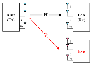
Figure 1: MIMO Gaussian wiretap channel with $n_{t}$, $n_{r}$, and $n_{e}$ antennas, at the transmitter (Alice), legitimate receiver (Bob), and eavesdropper (Eve).

Precoding is a technique for exploiting transmit diversity via weighting the information stream. Singular value decomposition (SVD) precoding with water-filling power allocation is a well-known example that achieves the capacity of the MIMO channel. Khisti and Wornell [4] proposed a generalized SVD (GSVD)-based precoding scheme with equal power allocation for the MIMO Gaussian wiretap channel. The optimal power allocation scheme for GSVD precoding in the MIMO Gaussian wiretap channel was obtained in [11]. Although GSVD precoding gets close to the capacity in certain antenna configurations, it is neither capacity-achieving nor very close to capacity, in general. Despite its importance and years of research, optimal transmit/receive strategies to maximize the secure rate in MIMO wiretap channels remain unknown, in general. Linear beamforming transmission has, however, been proved to be optimal for the special case of $n_{t}=2$, $n_{r}=2$, and $n_{e}=1$ in [12]. It is also known to be the optimal communication strategy for multiple-input single-output (MISO) wiretap channels [13, 14].

Recently, a closed-form solution for the optimal covariance matrix has been found when the channel is strictly degraded and another condition on the channel matrices, which is equivalent to a lower threshold on the transmitted power, holds [15, 16, 17]. The combination of this result and the unit-rank solution of [14] can give the optimal covariance matrix for the case of two transmit antennas [17]. The optimal solution is, however, still open in general.

In this paper, we characterize optimal precoding and power allocation for MIMO Gaussian wiretap channels in which the legitimate receiver and eavesdropper have arbitrary numbers of antennas but the transmitter has two antennas. This proves that linear beamforming transmission can be optimal for a much broader class of MIMO Gaussian wiretap channels. Our approach in finding the optimal covariance matrix is completely different from that of [16] and [17]. It does not require the degradedness condition and thus provides the optimal solution for both full-rank and rank-deficient cases in one shot. The proposed beamforming and power allocation schemes result in a computable capacity with a reasonably low complexity. It requires searching over two scalars (power allocation) at most. In addition, the proposed beamforming and power allocation schemes can bring notably high gain over GSVD-based beamforming, as confirmed by simulation results.

It is worth highlighting that the new precoding and power allocation techniques are applicable to and optimal for MIMO channels without secrecy, simply by setting the eavesdroppers channel to zero. In such cases, power allocation is even simpler and does not require a search.

Secure transmission strategies in multi-antenna networks with various constraints and/or in different settings, e.g., with energy-efficiency [18], finite memory [19], joint source-relay precoding [20], game-theoretic precoding[21], and varying eavesdropper channel states [22] have been considered recently.

The rest of the paper is organized as follows. In Section II, we describe the system model. In Section III, we reformulate the secrecy rate problem and propose linear precoding and power allocation schemes to achieve the capacity of the MIMO/MISO wiretap channels. In Section IV, we show that the proposed precoding and power allocation schemes are also optimal for MIMO/MISO channels without an eavesdropper and we discuss possible extensions of the proposed precoding method. We present numerical results in Section V before concluding the paper in Section VI.

Throughout this work, we use notations $\mathrm{tr}(\cdot)$, $\det(\cdot)$, $(\cdot)^{t}$, and $(\cdot)^{H}$ to denote the trace, determinant, transpose, and conjugate transpose of a matrix, respectively. Matrices are written in bold capital letters and vectors are written in bold small letters. $\mathbf{A}\succeq\mathbf{0}$ means that $\mathbf{A}$ is a positive semidefinite matrix, and $\mathbf{I}_{m}$ represents the identity matrix of size $m$.

II System Model and Preliminaries

Consider a MIMO Gaussian wiretap channel, in which a transmitter (Alice) wishes to communicate with a legitimate receiver (Bob) in the presence of an eavesdropper (Eve), as shown in Fig. 1. The nodes are equipped with $n_{t}$, $n_{r}$, and $n_{e}$ antennas, respectively. Let $\mathbf{H}\in\mathbb{R}^{n_{r}\times n_{t}}$ and $\mathbf{G}\in\mathbb{R}^{n_{e}\times n_{t}}$ be the channel matrices for the legitimate user and eavesdropper. Both channels are assumed to undergo independent and identically distributed (i.i.d.) Rayleigh fading, where the channel gains are real Gaussian random variables. The received signal at the legitimate receiver and eavesdropper are, respectively, given by

$$\mathbf{y}_{r}=\mathbf{H}\,\mathbf{x}\,+\,\mathbf{w}_{r},$$ (1a)

$$\mathbf{y}_{e}=\mathbf{G}\,\mathbf{x}\,+\,\mathbf{w}_{e},$$ (1b)

in which $\mathbf{x}\in\mathbb{R}^{n_{t}\times 1}$ is the transmitted signal and $\mathbf{w}_{i}\in\mathbb{R}^{n_{i}\times 1}$, $i\in\{r,e\}$, represents an i.i.d. Gaussian noise vector with zero mean and identity covariance matrix. As will be seen later, $\mathbf{x}=\mathbf{V}\mathbf{s}$ where $\mathbf{V}\in\mathbb{R}^{n_{t}\times n_{t}}$ is the precoding matrix to transmit a secrete data symbol vector $\mathbf{s}$. The transmitted signal is subject to an average power constraint

$$\mathrm{tr}(\mathbb{E}\{\mathbf{xx}^{t}\})=\mathrm{tr}(\mathbf{Q})\leq P,$$

where $P$ is a scalar, and $\mathbf{Q}=\mathbb{E}\{\mathbf{xx}^{t}\}$ is the input covariance matrix.

A single-letter expression for the secrecy capacity of the general discrete memoryless wiretap channel with transition probability $p(y_{r},y_{e}|x)$ is given by [24]

$$C_{s}=\max_{p(u,x)}\big{[}I(U;Y_{r})-I(U;Y_{e})\big{]},$$ (2)

in which the auxiliary random variable $U$ satisfies the Markov relation $U\rightarrow X\rightarrow(Y_{r},Y_{e}).$

With this, the problem of characterizing the secrecy capacity of the multiple-antenna wiretap channel reduces to evaluating (2) for the channel model given in (1). This was, however, open until the work of Khisti and Wornell [4] and Oggier and Hassibi [5], where they proved that $U=X$ is optimal in (2). Then, the secrecy capacity (bits per real dimension) is the solution of the following optimization problem [4, 5, 6]:

$$\max_{\mathbf{Q}} \frac{1}{2}\left[\log\det(\mathbf{I}_{n_{r}}\!\!+\mathbf{H}\mathbf{Q}\mathbf{H}^{t})-\log\det(\mathbf{I}_{n_{e}}\!\!+\mathbf{G}\mathbf{Q}\mathbf{G}^{t})\right]$$ (3)

$$\operatorname{s.t.} \mathbf{Q}\succeq\mathbf{0},\mathbf{Q}=\mathbf{Q}^{t},\;\mathrm{tr}(\mathbf{Q})\leq P,$$

in which the first two constraints are due to the fact that $\mathbf{Q}$ is a covariance matrix and the third constraint is the aforementioned average power constraint. The secrecy capacity is obviously nonnegative as $\mathbf{Q}=\mathbf{0}$ is a feasible solution of (LABEL:eq:cap0). The above optimization problem is non-convex (except for $n_{r}=n_{e}=1$ [25]) and its objective function possesses numerous local maxima [26, 8, 10]. As such, a closed-form solution for the optimum $\mathbf{Q}$ is not known, in general.

The problem of characterizing the optimal input covariance matrix that achieves secrecy capacity subject to a power constraint has been under active investigation recently [15, 16, 17, 27]. Until recently, the special cases for which the optimal $\mathbf{Q}$ was known were limited to the cases of $n_{r}=1$[14] and $n_{t}=2$, $n_{r}=2$, $n_{e}=1$ [12]. More recently, major steps have been made in characterizing the optimal covariance matrix. Fakoorian and Swindlehurst [16] determined conditions under which the optimal input covariance matrix is full-rank or rank-deficient. They also fully characterized the optimal $\mathbf{Q}$ when it is full-rank. Very recently, Loyka and Charalambous [17] found a closed-form solution for the optimal covariance matrix when the channel is strictly degraded ($\mathbf{H}^{H}\mathbf{H}\succ\mathbf{G}^{H}\mathbf{G}$) and transmission power is greater than a certain value. The combination of this result and the unit-rank solution of [4] gives the optimal $\mathbf{Q}$ for the rank-2 case [17]. The optimal solution is, however, still open in general.

In this paper, we study the MIMO wiretap channel with $n_{t}=2$ while $n_{r}$ and $n_{e}$ are arbitrary integers. We derive a closed-form solution for the optimal covariance matrix in this case. Our approach is completely different from that of [16] and [17]. In addition, unlike [16] and [17], our approach does not require finding the rank of the optimal covariance matrix before fully characterizing the solution. It gives the optimal solution for both full-rank and rank-deficient cases in one shot. What is more, in [17], it is not clear when the rank of the optimal solution switches from one to two (i.e., the paper does not clarify at what power threshold this change of rank happens); thus, it is not known whether a rank-one solution or full-rank solution should be applied.

III A Capacity Achieving Precoding

Based on the optimization problem in (LABEL:eq:cap0), a characterization of the secrecy capacity of the MIMO Gaussian wiretap channel is given by non-negative $R$ such that

$$R \leq\max_{\mathbf{Q}}\frac{1}{2}\left[\log\det(\mathbf{I}_{n_{r}}\!\!+\mathbf{H}\mathbf{Q}\mathbf{H}^{t})-\log\det(\mathbf{I}_{n_{e}}\!\!+\mathbf{G}\mathbf{Q}\mathbf{G}^{t})\right]$$

$$=\max_{\mathbf{Q}}\frac{1}{2}\log\frac{\det(\mathbf{I}_{n_{t}}\!\!+\mathbf{H}^{t}\mathbf{H}\mathbf{Q})}{\det(\mathbf{I}_{n_{t}}\!\!+\mathbf{G}^{t}\mathbf{G}\mathbf{Q})},$$ (4)

where $\mathbf{Q}\succeq\mathbf{0},\mathbf{Q}=\mathbf{Q}^{t},\mathrm{tr}(\mathbf{Q})\leq P$. The equality in (III) is due to the fact that for any $\mathbf{A}\in\mathbb{C}^{m\times n}$ and $\mathbf{B}\in\mathbb{C}^{n\times m}$ we have

$$\det(\mathbf{I}_{m}+\mathbf{A}\mathbf{B})=\det(\mathbf{I}_{n}+\mathbf{B}\mathbf{A}).$$ (5)

Note that $\mathbf{H}^{t}\mathbf{H}$ and $\mathbf{G}^{t}\mathbf{G}$ are $n_{t}\times n_{t}$ symmetric matrices. Also, $\mathbf{Q}$ is an $n_{t}\times n_{t}$ symmetric matrix and its eigendecomposition can be written as

$$\mathbf{Q}=\mathbf{V}\mathbf{\Lambda}\mathbf{V}^{t},$$ (6)

where $\mathbf{V}\in\mathbb{R}^{n_{t}\times n_{t}}$ is the orthogonal matrix whose $i$th column is the $i$th eigenvector of $\mathbf{Q}$ and $\mathbf{\Lambda}$ is the diagonal matrix whose diagonal elements are the corresponding eigenvalues, i.e., $\mathbf{\Lambda}_{ii}=\lambda_{i}$. In this paper, we study the case where $n_{t}=2$ while $n_{r}$ and $n_{e}$ are arbitrary integers.

III-A Reformulating the Problem for $n_{t}=2$

We simplify the optimization problem (III) for $n_{t}=2$ in this subsection. Since $\mathbf{V}$ is orthogonal its columns are orthonormal and, without loss of generality, we can write

$$\mathbf{V}=\left[\begin{matrix}-\sin\theta&\cos\theta\\ \cos\theta&\sin\theta\end{matrix}\right],$$ (7)

for some $\theta$. Further, let

$$\mathbf{H}^{t}\mathbf{H}=\left[\begin{matrix}h_{1}&h_{2}\\ h_{2}&h_{3}\end{matrix}\right],\quad\mathbf{G}^{t}\mathbf{G}=\left[\begin{matrix}g_{1}&g_{2}\\ g_{2}&g_{3}\end{matrix}\right].$$ (8)

The following lemma converts the optimization problem (III) into a more tractable problem.

Lemma 1.

For $n_{t}=2$ but arbitrary $n_{r}$ and $n_{e}$, the optimization problem in (III) is equivalent to

$$R\leq\max_{\lambda_{1}+\lambda_{2}\leq P}\frac{1}{2}\log\left(\frac{a_{1}\sin 2\theta+b_{1}\cos 2\theta+c_{1}}{a_{2}\sin 2\theta+b_{2}\cos 2\theta+c_{2}}\right),$$ (9)

in which $\lambda_{1}$ and $\lambda_{2}$ are nonnegative, and

$$a_{1} =(\lambda_{2}-\lambda_{1})h_{2},$$ (10a)

$$b_{1} =\frac{1}{2}(\lambda_{1}-\lambda_{2})(h_{3}-h_{1}),$$ (10b)

$$c_{1} =1+\frac{1}{2}(\lambda_{1}+\lambda_{2})(h_{1}+h_{3})+\lambda_{1}\lambda_{2}(h_{1}h_{3}-h_{2}^{2}),$$ (10c)

and

$$a_{2} =(\lambda_{2}-\lambda_{1})g_{2},$$ (11a)

$$b_{2} =\frac{1}{2}(\lambda_{1}-\lambda_{2})(g_{3}-g_{1}),$$ (11b)

$$c_{2} =1+\frac{1}{2}(\lambda_{1}+\lambda_{2})(g_{1}+g_{3})+\lambda_{1}\lambda_{2}(g_{1}g_{3}-g_{2}^{2}).$$ (11c)

Proof.

To prove this lemma, we simplify the determinants in (III). First, consider $\det(\mathbf{I}_{n_{t}}+\mathbf{H}^{t}\mathbf{H}\mathbf{Q})$. Using $\mathbf{Q}$ given in (6) and applying (5), it is seen that $\det(\mathbf{I}_{n_{t}}+\mathbf{H}^{t}\mathbf{H}\mathbf{Q})=\det(\mathbf{I}_{n_{t}}+\mathbf{V}^{t}\mathbf{H}^{t}\mathbf{H}\mathbf{V}\mathbf{\Lambda}).$ Further, it is straightforward to check that

$$\mathbf{V}^{t}\mathbf{H}^{t}\mathbf{H}\mathbf{V}=\left[\begin{matrix}w_{1}&w_{2}\\ w_{2}&w_{3}\end{matrix}\right],$$ (12)

in which

$$w_{1} =h_{1}\sin^{2}\theta+h_{3}\cos^{2}\theta-2h_{2}\sin\theta\cos\theta,$$ (13a)

$$w_{2} =h_{2}(\cos^{2}\theta-\sin^{2}\theta)+(h_{3}-h_{1})\sin\theta\cos\theta,$$ (13b)

$$w_{3} =h_{1}\cos^{2}\theta+h_{3}\sin^{2}\theta+2h_{2}\sin\theta\cos\theta.$$ (13c)

Consequently,

$$\det(\mathbf{I}_{n_{t}}+\mathbf{H}^{t}\mathbf{H}\mathbf{Q}) =\det(\mathbf{I}_{n_{t}}+\mathbf{V}^{t}\mathbf{H}^{t}\mathbf{H}\mathbf{V}\mathbf{\Lambda})$$ (14)

$$=(1+\lambda_{1}w_{1})(1+\lambda_{2}w_{3})-\lambda_{1}\lambda_{2}w_{2}^{2}.$$

Next, using the basic trigonometric identities

$$\cos 2\theta =2\cos^{2}\theta-1=1-2\sin^{2}\theta,$$ (15a)

$$\sin 2\theta =2\sin\theta\cos\theta,$$ (15b)

it is straightforward to show that

$$w_{1} =\frac{h_{1}+h_{3}}{2}+\frac{h_{3}-h_{1}}{2}\cos 2\theta-h_{2}\sin 2\theta,$$ (16a)

$$w_{2} =h_{2}\cos 2\theta+\frac{h_{3}-h_{1}}{2}\sin 2\theta,$$ (16b)

$$w_{3} =\frac{h_{1}+h_{3}}{2}-\frac{h_{3}-h_{1}}{2}\cos 2\theta+h_{2}\sin 2\theta.$$ (16c)

Substituting (16a)-(16c) in (14), we obtain

$$\det(\mathbf{I}_{n_{t}}+\mathbf{H}^{t}\mathbf{H}\mathbf{Q}) =a_{1}\sin 2\theta+b_{1}\cos 2\theta+c_{1},$$ (17)

in which $a_{1}$, $b_{1}$, and $c_{1}$ are given in (10). Following similar steps it is clear that

$$\det(\mathbf{I}_{n_{t}}+\mathbf{G}^{t}\mathbf{G}\mathbf{Q})=a_{2}\sin 2\theta+b_{2}\cos 2\theta+c_{2},$$ (18)

where $a_{2}$, $b_{2}$, and $c_{2}$ are given in (11). It should be mentioned that the constraint $\lambda_{1}+\lambda_{2}\leq P$ comes from $\mathrm{tr}(\mathbf{Q})\leq P$ since, from (6), $\mathrm{tr}(\mathbf{Q})=\mathrm{tr}(\mathbf{V}\mathbf{\Lambda}\mathbf{V}^{t})=\mathrm{tr}(\mathbf{V}^{t}\mathbf{V}\mathbf{\Lambda})=\mathrm{tr}(\mathbf{\Lambda}).$ Note that $\mathrm{tr}(\mathbf{AB})=\mathrm{tr}(\mathbf{BA})$ and $\mathbf{V}^{t}\mathbf{V}=\mathbf{I}_{n_{t}}$. Also, $\lambda_{1}\geq 0$ and $\lambda_{2}\geq 0$ are due to $\mathbf{Q}\succeq\mathbf{0}$. This completes the proof of Lemma 1. ∎

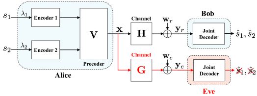
Figure 2: Optimal architecture for communicating over the MIMO Gaussian wiretap channel with $n_{t}=2$ and arbitrary $n_{r}$ and $n_{e}$.

Lemma 2.

In the optimization problem given by Lemma 1, the constraint $\lambda_{1}+\lambda_{2}\leq P$ can be replaced either by $\lambda_{1}+\lambda_{2}=P$ or $\lambda_{1}+\lambda_{2}=0$; i.e., it is optimal to use either all available power or nothing.

Proof.

See Appendix A. ∎

III-B Optimal Precoding

In what follows, we first find a closed-form solution for the optimization problem in Lemma 1 for a given pair of $\lambda_{1}$ and $\lambda_{2}$ that satisfy the constraints. Since $\log(x)$ is strictly increasing in $x$, we can instead maximize the argument of the logarithm in (9). Thus, let us define

$$W=\frac{a_{1}\sin 2\theta+b_{1}\cos 2\theta+c_{1}}{a_{2}\sin 2\theta+b_{2}\cos 2\theta+c_{2}}.$$ (19)

Then, $\theta^{*}=\arg\max W$ and is obtained by differentiating $W$ with respect to $\theta$ and finding its critical points. It can be checked that $\frac{\partial W}{\partial\theta}=0$ is equivalent to

$$a\sin 2\theta+b\cos 2\theta+c=0,$$ (20)

in which

$$a =c_{1}b_{2}-c_{2}b_{1},$$ (21a)

$$b =a_{1}c_{2}-a_{2}c_{1},$$ (21b)

$$c =a_{1}b_{2}-a_{2}b_{1}.$$ (21c)

Before proceeding, we note that $W$ is periodic in $\theta$ and its period is $\pi$. Also, it can be checked that if both $a$ and $b$ are zero, then $\frac{a_{1}}{a_{2}}=\frac{b_{1}}{b_{2}}=\frac{c_{1}}{c_{2}}$ and $W$ is constant; i.e., any $\theta$ is optimal. Thus, we assume $a^{2}+b^{2}\neq 0.$ Defining $\frac{b}{a}=\tan\phi$, (20) can be further simplified as

$$\sin(2\theta+\phi)+\frac{c}{\sqrt{a^{2}+b^{2}}}=0.$$ (22)

The critical points of the above equation are given by

$$2\theta=\begin{cases}-\arctan\frac{b}{a}-\arcsin\frac{c}{\sqrt{a^{2}+b^{2}}}+2k\pi\\ -\arctan\frac{b}{a}+\pi+\arcsin\frac{c}{\sqrt{a^{2}+b^{2}}}+2k\pi\\ \end{cases},$$ (23)

where $k$ is an integer. Then, using the second derivative of $W$ with respect to $\theta$, we can verify that the first argument gives the minimum of $W$ while the second one gives its maximum. For completeness, this is proved in Appendix B. Further, without loss of optimality, we let $k=0$ in (23). Hence, the optimal $\theta$ that maximizes $W$ is obtained by

$$\theta^{*}=-\frac{1}{2}\arctan\frac{b}{a}+\frac{1}{2}\arcsin\frac{c}{\sqrt{a^{2}+b^{2}}}+\frac{\pi}{2}.$$ (24)

Thus far, the optimal $\theta$ is obtained for given $\lambda_{1}$ and $\lambda_{2}$. To find the optimal $\lambda_{1}$ and $\lambda_{2}$, in light of Lemma 2, we can search over all $\lambda_{1}\geq 0$ and $\lambda_{2}\geq 0$ that satisfy $\lambda_{1}+\lambda_{2}=P$ or $\lambda_{1}+\lambda_{2}=0$ and maximize (19) where $\theta$ is given in (24). We can vary $\lambda_{1}$ from $0$ to $P$. Therefore, we have the following.

Theorem 1.

To achieve the secrecy capacity of the MIMO Gaussian wiretap channel (with $n_{t}=2$) under the average power constraint $P$, it suffices to use

$$\mathbf{V}=\left[\begin{matrix}-\sin\theta&\cos\theta\\ \cos\theta&\sin\theta\end{matrix}\right],$$ (25)

as the transmit beamformer with the power allocation matrix

$$\mathbf{\Lambda}=\left[\begin{matrix}\lambda_{1}&0\\ 0&\lambda_{2}\end{matrix}\right].$$ (26)

An optimal $\theta$ is given by (24) and is obtained by searching over nonnegative $\lambda_{1}$ and $\lambda_{2}$ that satisfy $\lambda_{1}+\lambda_{2}=P$ or $\lambda_{1}+\lambda_{2}=0$ and maximize (19).

Once the optimal $\mathbf{V}$, $\lambda_{1}$, and $\lambda_{2}$ are determined, these can be used for precoding and power allocation as illustrated in Fig 2, similarly to the V-BLAST architecture for communicating over the MIMO channel [23]. Here, two ($n_{t}=2$) independent data streams are multiplexed in the coordinate system given by the precoding matrix $\mathbf{V}$. The $i$th data stream is allocated a power $\lambda_{i}$. Each stream is encoded using a capacity-achieving Gaussian code. The data streams are decoded jointly. When the orthogonal matrix $\mathbf{V}$ and powers $\lambda_{i}$ are chosen as described in Theorem 1, then we have the capacity-achieving architecture in Fig 2.

Lemma 3.

With a proper choice of $\theta$, the pairs $(\lambda_{1},\lambda_{2})$ and $(\lambda_{2},\lambda_{1})$ result in the same maximum rate in Lemma 1.

Proof.

See Appendix C. ∎

This lemma implies that to find optimal $(\lambda_{1},\lambda_{2})$ in Theorem 1, it suffices to search for $\lambda_{1}$ in $[0\;\frac{P}{2}]$ rather than $[0\;P]$.

III-C Special Cases

The first special case of the MIMO Gaussian wiretap channel we consider is the MISO Gaussian wiretap channel. In the following corollary, we prove that a positive capacity for the MISO case is obtained by signaling with rank one covariance. This has already been shown in [14] using a different argument.

Corollary 1.

For the MISO Gaussian wiretap channel, Theorem 1 significantly simplifies and ($\lambda_{1},\lambda_{2})=(0,P)$ or ($\lambda_{1},\lambda_{2})=(0,0)$ is the optimal solution. The optimal $\theta$ is then obtained from (24).

Proof.

In the case of the MISO multi-eavesdropper wiretap channel it is known that the rank of the covariance matrix is either one or zero (see [14, Theorem 2] or [17]). In the latter case, it is trivial that ($\lambda_{1},\lambda_{2})=(0,0)$ is an optimal solution. In the former case, from Theorem 1 we can see that a rank-one solution implies that either $\lambda_{1}$ or $\lambda_{2}$ is equal to zero. Then, from Lemma 2 we conclude that ($\lambda_{1},\lambda_{2})=(P,0)$ or ($\lambda_{1},\lambda_{2})=(0,P)$. But, in view of Lemma 3, we know that with proper choice of $\theta$ these two cases result in the same maximum rates; thus, one of them can be removed. ∎

Another special case of the MIMO Gaussian wiretap channel is the case in which the eavesdropper has only one antenna. Specifically, by setting $n_{e}=1$ in Theorem 1 we get

Corollary 2.

For the $2$-$n_{r}$-$1$ Gaussian wiretap channel, optimal transmit covariance matrix is at most unit-rank. In particular, either ($\lambda_{1},\lambda_{2})=(0,P)$ or ($\lambda_{1},\lambda_{2})=(0,0)$ gives the optimal solution in Theorem 1.

Proof.

The proof is very similar to that of Corollary 1 and is omitted. Note that the objective function, in this case, is in the form of the inverse of that of Corollary 1.∎

Note that Corollary 1 gives the capacity of $2$-$n_{r}$-$1$ channels and thus generalizes the result of [12] for the $2$-$2$-$1$ channel.

III-D Closed-Form Solution for Optimal Power Allocation

Finding optimal $\lambda_{1}$ and $\lambda_{2}$ in Theorem 1 requires an exhaustive search. Although checking a reasonably small number of ($\lambda_{1}$, $\lambda_{2}$) is enough in practice, in this subsection we find a closed-form solution for optimal ($\lambda_{1}$, $\lambda_{2}$).

We know that if $W\leq 1$ then $(\lambda^{*}_{1},\lambda^{*}_{2})=(0,0)$ is the optimal solution. Thus, let us assume $W>1$. Then, using Lemma 2, this implies that $\lambda_{1}+\lambda_{2}=P$ is optimal. Thus, to find optimal $\lambda_{1}$ and $\lambda_{2}$, we can solve the following problem:

$$\mathcal{C}_{\mathrm{MIMOME}}=\max_{\lambda_{1}+\lambda_{2}=P}\frac{1}{2}\log(W),$$ (27)

where $W=\det(\mathbf{I}_{n_{t}}+\mathbf{H}^{t}\mathbf{H}\mathbf{Q})/\det(\mathbf{I}_{n_{t}}\!\!+\mathbf{G}^{t}\mathbf{G}\mathbf{Q})$ is given in (III). To this end, we define $a_{h}\triangleq\frac{h_{3}-h_{1}}{2},b_{h}\triangleq-h_{2},$ $c_{h}\triangleq\frac{h_{1}+h_{3}}{2},d_{h}\triangleq\sqrt{a_{h}^{2}+b_{h}^{2}},$ and $\frac{b_{h}}{a_{h}}\triangleq\tan\phi_{h}$. Then, from (16a)-(16c) we will have

$$w_{1} =c_{h}+d_{h}\cos(2\theta-\phi_{h}),$$ (28a)

$$w_{2} =d_{h}\sin(2\theta-\phi_{h}),$$ (28b)

$$w_{3} =c_{h}-d_{h}\cos(2\theta-\phi_{h}).$$ (28c)

Now, we can write

$$W_{h} =\det(\mathbf{I}_{n_{t}}\!\!+\mathbf{H}^{t}\mathbf{H}\mathbf{Q})$$

$$\stackrel{{\scriptstyle(a)}}{{=}}(1+\lambda_{1}w_{1})(1+\lambda_{2}w_{3})-\lambda_{1}\lambda_{2}w_{2}^{2}$$

$$=1+\lambda_{1}w_{1}+\lambda_{2}w_{3}+\lambda_{1}\lambda_{2}(w_{1}w_{3}-w_{2}^{2})$$

$$\stackrel{{\scriptstyle(b)}}{{=}}1+\lambda_{1}w_{1}+\lambda_{2}w_{3}+\lambda_{1}\lambda_{2}(h_{1}h_{3}-h_{2}^{2})$$

$$\stackrel{{\scriptstyle(c)}}{{=}}1+(\lambda_{1}\!+\!\lambda_{2})c_{h}+(\lambda_{1}\!-\!\lambda_{2})d_{h}\cos(2\theta-\phi_{h})$$

$$\quad+\lambda_{1}\lambda_{2}(h_{1}h_{3}-h_{2}^{2}),$$

$$\stackrel{{\scriptstyle(d)}}{{=}}1+Pc_{h}+(2\lambda_{1}-P)d_{h}\cos(2\theta-\phi_{h})$$

$$\quad+\lambda_{1}(P-\lambda_{1})(h_{1}h_{3}-h_{2}^{2})$$

$$\stackrel{{\scriptstyle(e)}}{{=}}\alpha_{h}+\beta_{h}\lambda_{1}-\delta_{h}\lambda_{1}^{2},$$ (29)

in which $(a)$ is due to (14), $(b)$ can be verified using (16a)-(16c), $(c)$ is due to (28a) and (28c), $(d)$ is due to the fact that $\lambda_{1}+\lambda_{2}=P$ is optimal when $W>1$, which follows from Lemma 2, and $(e)$ is obtained by defining

$$\alpha_{h} =1+Pc_{h}-Pd_{h}\cos(2\theta-\phi_{h}),$$ (30a)

$$\beta_{h} =2d_{h}\cos(2\theta-\phi_{h})+P\delta_{h},$$ (30b)

$$\delta_{h} =h_{1}h_{3}-h_{2}^{2}.$$ (30c)

In a similar way, we can show that

$$W_{g} =\det(\mathbf{I}_{n_{t}}\!\!+\mathbf{G}^{t}\mathbf{G}\mathbf{Q})=\alpha_{g}+\beta_{g}\lambda_{1}-\delta_{g}\lambda_{1}^{2},$$ (31)

where

$$\alpha_{g} =1+Pc_{g}-Pd_{g}\cos(2\theta-\phi_{g}),$$ (32a)

$$\beta_{g} =2d_{g}\cos(2\theta-\phi_{g})+P\delta_{g},$$ (32b)

$$\delta_{g} =g_{1}g_{3}-g_{2}^{2},$$ (32c)

and $c_{g},d_{g}$, and $\phi_{g}$ are defined for $\mathbf{G}$ similarly to those of $\mathbf{H}$. Hence, we can write

$$W =\frac{W_{h}}{W_{g}}=\frac{\alpha_{h}+\beta_{h}\lambda_{1}-\delta_{h}\lambda_{1}^{2}}{\alpha_{g}+\beta_{g}\lambda_{1}-\delta_{g}\lambda_{1}^{2}}.$$ (33)

Next, it can be checked that

$$\frac{\partial W}{\partial\lambda_{1}}=\frac{\bar{c}+\bar{b}\lambda_{1}+\bar{a}\lambda_{1}^{2}}{(\alpha_{g}+\beta_{g}\lambda_{1}-\delta_{g}\lambda_{1}^{2})^{2}},$$ (34)

in which

$$\bar{a} =\delta_{g}\beta_{h}-\delta_{h}\beta_{g},$$ (35a)

$$\bar{b} =2\delta_{g}\alpha_{h}-2\delta_{h}\alpha_{g},$$ (35b)

$$\bar{c} =\beta_{h}\alpha_{g}-\beta_{g}\alpha_{h}.$$ (35c)

Let $\Delta=\bar{b}^{2}-4\bar{a}\bar{c}$, and suppose that $\Delta>0$. Then

$$\lambda_{1,1}^{*}=(-\bar{b}+\sqrt{\Delta})/2\bar{a},$$ (36a)

$$\lambda_{1,2}^{*}=(-\bar{b}-\sqrt{\Delta})/2\bar{a},$$ (36b)

are the roots of (34). Next, it is easy to show that, for $\lambda_{1,i}^{*},\;i\in\{1,2\}$, in (36a) and (36b) we have

$$\frac{\partial^{2}W}{\partial\lambda_{1}^{2}}(\lambda_{1,i}^{*}) =\frac{\bar{b}+2\bar{a}\lambda_{1,i}^{*}}{(\alpha_{g}+\beta_{g}\lambda_{1}-\delta_{g}\lambda_{1}^{2})^{2}}=\begin{cases}+\frac{\sqrt{\Delta}}{W_{g}^{2}},\qquad i=1\\ -\frac{\sqrt{\Delta}}{W_{g}^{2}},\qquad i=2\\ \end{cases}\!\!\!\!\!\!.$$ (37)

That is, the second derivative is positive at $\lambda_{1,1}^{*}$ and negative at $\lambda_{1,2}^{*}$. Thus, the former corresponds to a minimum of $W$ and the latter corresponds to a maximum of that quantity. Therefore, the following cases appear:

III-D1 Case I ($\Delta\leq 0)$

This case results in a strictly decreasing or increasing $W$ in $\lambda_{1}$. Then, $\lambda_{1}=0$ or $\lambda_{1}=P$ is optimal, depending on the sign of $a$. The optimum value of $\lambda_{1}$ can be inserted into (10) and (11) to find the optimal $\theta$. The optimal $\lambda_{2}$ is obtained from $\lambda_{1}+\lambda_{2}=P$.

III-D2 Case II ($\Delta>0)$

In this case, the maximum of $W$ is achieved by $\lambda_{1}=0$, $\lambda_{1}=P$, or $\lambda_{1}=\lambda_{1,2}^{*}$, provided that $0\leq\lambda_{1,2}^{*}\leq P$. The optimal $\lambda_{2}$ is obtained from $\lambda_{1}+\lambda_{2}=P$. Hence, when $W>1$, $(\lambda^{*}_{1},\lambda^{*}_{2})$ is one of the following pairs: $(0,P)$, $(P,0)$, or $(\lambda_{1,2}^{*},P-\lambda_{1,2}^{*})$. But, in light of Lemma 3, it can be seen that $(0,P)$ and $(P,0)$ result in the same optimum $W$ and thus one of them can be omitted.

To summarize, considering all cases for $W\leq 1$ and $W>1$, it is enough to check

$$(\lambda^{*}_{1},\lambda^{*}_{2}) =(0,0),$$ (38a)

$$(\lambda^{*}_{1},\lambda^{*}_{2}) =(0,P),$$ (38b)

$$(\lambda^{*}_{1},\lambda^{*}_{2}) =(\lambda_{1,2}^{*},P-\lambda_{1,2}^{*}),$$ (38c)

in order to obtain the maximum of $W$. We should highlight that (38c) will be a choice only if $\lambda_{1,2}^{*}$, defined in (36b), is a real number between $0$ and $P$. As a result, we have

Theorem 2.

The optimal $\lambda_{1}$ and $\lambda_{2}$ in Theorem 1 is confined to one of the following cases:

$$(\lambda_{1},\lambda_{2})=\begin{cases}(0,0),\qquad\;\\ (0,P),\qquad\\ (\lambda^{*},P-\lambda^{*}),\qquad\\ \end{cases},$$ (39)

in which $\lambda^{*}\triangleq\lambda_{1,2}^{*}$ is defined in (36b), and $\theta$ is given in (24).

Remark 1.

As can be traced from (36b), in general, the optimal $\lambda_{1}$ is a function of $\theta$. On the other hand, the optimal $\theta$, given in (24), is a function of $\lambda_{1}$ (and $\lambda_{2}$). Thus, the triplet $(\lambda_{1},\lambda_{2},\theta)$ can be found for any possible maximizing argument in (39). Then, by evaluating $W$ for these points we can determine which one is the optimal (capacity-achieving) solution. For the first two cases in (39) the solution is obtained analytically. However, the equation resulting from combining the third case in (39) and (24) is rather cumbersome and thus we solve it numerically.

IV Special Cases and Possible Extensions

In this section, we briefly consider some special cases of the proposed precoding as well as possible extensions of this work.

IV-A Beamforming for MISO and MIMO Channels

The optimal beamforming provided in the previous section achieves the capacity of MISO and MIMO channels without an eavesdropper ($\mathbf{G}=\mathbf{0}$), as shown below.

IV-A1 Capacity of MISO Channels

We know that the capacity of a MISO channel is given by [23]

$$\mathcal{C}_{\mathrm{MISO}}=\frac{1}{2}\log(1+\|\mathbf{h}\|^{2}P),$$ (40)

where $\mathbf{h}$ is the channel vector. On the other hand, using (14), it is straightforward to check that the above rate is achieved by letting $\lambda_{1}=P$, $\lambda_{2}=0$, and $\theta=\frac{\pi}{2}+\alpha$, where $\tan\alpha\triangleq\frac{\sqrt{h_{3}}}{\sqrt{h_{1}}}$.

IV-A2 Capacity of MIMO Channels

It can be also checked that the proposed beamforming and power allocation is equal to SVD-based beamforming with water-filling for $\theta=\frac{1}{2}\tan^{-1}\frac{b_{h}}{a_{h}}$ and

$$\lambda_{1}=\min\Big{\{}\frac{P}{2}+\frac{c_{h}}{\delta_{h}},P\Big{\}},$$ (41a)

$$\lambda_{2}=\max\Big{\{}\frac{P}{2}-\frac{c_{h}}{\delta_{h}},0\Big{\}},$$ (41b)

where $a_{h}=\frac{h_{1}-h_{3}}{2}$, $b_{h}=h_{2}$, $c_{h}=\sqrt{a_{h}^{2}+b_{h}^{2}}$, and $\delta_{h}=h_{1}h_{1}-h_{2}^{2}$.

IV-B Extension to $n_{t}>2$

The key idea in this paper is to use the fact that any orthogonal matrix $\mathbf{V}$ is parametrized by a single parameter $\theta$, as shown in (7). Considering this, in (III), we rewrite the capacity expression in a way that for any $n_{r}$ and $n_{e}$ (with $n_{t}=2$) the terms $\mathbf{H}^{t}\mathbf{H}$ and $\mathbf{G}^{t}\mathbf{G}$ are $2\times 2$ matrices. Hence, the capacity expression can be represented by three parameters, two nonnegative powers ($\lambda_{1}$ and $\lambda_{2}$) and one angle $\theta$. Then, the covariance matrix can be optimized with elementary trigonometric equations, as shown in Section III. In the case of $n_{t}=3$, the main difficulty is to parametrize the $3\times 3$ orthogonal matrix $\mathbf{V}$ with two parameters. Even with this, it is not guaranteed to get a tractable optimization problem. We have made some progress towards this goal, but the resulting optimization problem is rather cumbersome and needs further simplification. This issue becomes more challenging as $n_{t}$ increases.

IV-C Construction of Practical Codes

Although the capacity of the MIMO wiretap channel is well-studied, construction of practical codes is still a challenging issue for this channel. Recently, it has been shown in [28] that a good wiretap code, e.g., a scalar random-binning code [29], is applicable to the MIMO wiretap channel in conjunction with a linear encoder and a successive interference cancellation (SIC) decoder to achieve a rate close to the MIMO wiretap capacity. However, this approach gives rise to several practical issues in terms of implementation, such as dithering in the SIC decoder. Considering this, one direction for future work would be to find a more practical code construction for MIMO wiretap channels based on our new design of closed-form optimal beamforming and power allocation solutions.

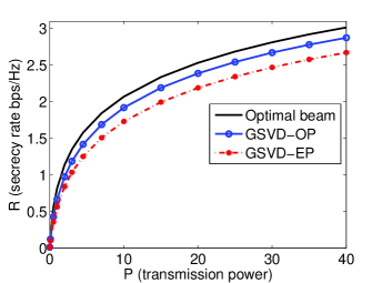
(a) $n_{e}=1$

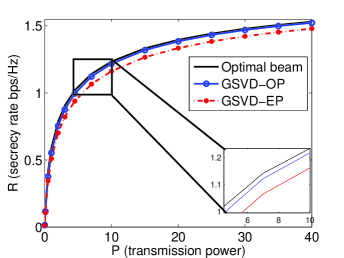
(b) $n_{e}=2$

Figure 3: Comparison of the secrecy capacity of the MIMO Gaussian wiretap channel (achieved by the proposed beamforming method) and the secrecy rate of GSVD-based beamforming with equal and optimal power allocations for (a) $n_{t}=2$, $n_{r}=2$, $n_{e}=1$ (b) $n_{t}=2$, $n_{r}=2$, $n_{e}=2$.

V Numerical Results

In this section, we provide numerical examples to illustrate the secrecy capacity of Gaussian multi-antenna wiretap channels using the proposed beamforming method. We also compare our results with those of GSVD-based beamforming with equal power (GSVD-EP) and optimal power (GSVD-OP) allocation proposed in [4] and [11], respectively. As proved in Section III, the proposed beamforming method is optimal and gives the capacity. Numerical results are included here to show how much gain this optimal method brings when compared with the existing beamforming and power allocation methods. It should be highlighted that the rate achieved by GSVD-OP is equal to or better than that of GSVD-EP, for any $\mathbf{H}$ and $\mathbf{G}$.

All simulation results are for 1000 independent realizations of the channel matrices $\mathbf{H}$ and $\mathbf{G}$. The entries of these matrices are generated by i.i.d. $\mathcal{N}(0,1)$. To get the capacity, we use the optimal power allocation of Theorem 2. We plot the secrecy rate versus total average power.

We first consider the case with $n_{t}=2$, $n_{r}=2$, and $n_{e}=1$, where the eavesdropper has only one antenna. As can be seen from Fig. 3(a), the capacity-achieving beamforming performs significantly better than both GSVD-based beamformings. By doubling the eavesdropper’s number of antennas in Fig. 3(b), the secrecy capacity nearly halves. Moreover, the rate achieved by the GSVD-OP becomes very close to that of optimal method. However, as can be seen in Fig. 3(b), there is still a small gap between the two methods particularly when $P$ is small.

We next consider the MISO wiretap channel in Fig. 4. It can be seen that there is a visible gap between the proposed beamforming and GSVD-based beamforming. Note that GSVD-EP and GSVD-OP have exactly the same performance for MISO wiretap channels. This is because there is only one beam and all power is allocated to that. A general trend was seen both for MISO and MIMO wiretap channels is that as SNR increases the performance of GSVD-EP, and thus GSVD-OP, get closer to that of the optimal beamforming scheme derived in this paper. This is not surprising knowing that GSVD-EP is asymptotically optimal; i.e., it is capacity-achieving as $P\to\infty$ [4].

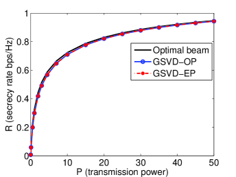
Figure 4: The secrecy capacity of the MISO wiretap channel and the secrecy rate of GSVD-based beamforming for $n_{t}=2$, $n_{r}=1$, and $n_{e}=2$.

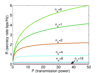
Figure 5: The secrecy capacity of the MIMO Gaussian wiretap channel for various $n_{e}$, with $n_{t}=2$, and $n_{r}=4$.

Figure 5 demonstrates the effect of increasing the number of antennas at the eavesdropper. All curves in this figure are for $n_{t}=2$, $n_{r}=4$ but a different number of eavesdropper antennas, as depicted on each curve. Note that $n_{e}=0$ refers to the case where there is no eavesdropper; this curve is basically the capacity of MIMO channel. Once the eavesdropper comes in play ($n_{e}\geq 1$), the extent to which information can be secured over the air reduces. The gap between each curve and the curve corresponding to $n_{e}=0$ is the unsecured information. Unfortunately, for $n_{e}=16$, and thus $n_{e}>16$, no information can be secured via physical layer techniques. This is because the eavesdropper can no longer be degraded by beamforming in this situation.

VI Conclusion

We have developed a linear precoding scheme to achieve the capacity of Gaussian multi-antenna wiretap channels in which the legitimate receiver and eavesdropper have arbitrary numbers of antennas but the transmitter has two antennas. We have reformulated the problem of determining the secrecy capacity into a tractable form and solved this new problem to find the corresponding optimal precoding and power allocation schemes. Our investigation leads to a computable capacity with reasonably small complexity. The gap between the secrecy rate achieved by the proposed precoding and GSVD-based beamforming can be remarkably high depending on the antenna configurations. When the legitimate receiver or eavesdropper has a single antenna, the optimal transmission scheme is unit-rank, i.e., beamforming is optimal. Further, in the absence of the eavesdropper, the proposed precoding reduces to the capacity-achieving scheme of the MIMO/MISO channels. Hence, it can be used for these channels with/without an eavesdropper.

Appendix A: Proof of Lemma 2

Proof.

Consider the optimization problem in (LABEL:eq:cap0). The secrecy capacity is zero if $\mathbf{H}^{t}\mathbf{H}-\mathbf{G}^{t}\mathbf{G}\preceq 0$ [5]. In this case, it is clear that $(\lambda_{1},\lambda_{2})=(0,0)$ is optimal. Otherwise, the secrecy capacity is strictly positive [5] and $\lambda_{1}+\lambda_{2}=P$ is optimal. This completes the proof since the optimization problem in Lemma 1 is a different representation of (LABEL:eq:cap0). ∎

Appendix B

To prove that the first (second) argument in (23) corresponds to the minimum (maximum), it suffices to show that the second derivative of $W$ is positive for the first argument and negative for the second one. Let $\beta\triangleq\arcsin\frac{c}{\sqrt{a^{2}+b^{2}}}$ and recall that $\beta\in[-\frac{\pi}{2}\;\frac{\pi}{2}]$. Then, form (23), the critical points are given by $\theta_{1}$ and $\theta_{2}$ where

$$\theta_{1} \triangleq-\frac{1}{2}\phi-\frac{1}{2}\beta+k\pi,$$ (42a)

$$\theta_{2} \triangleq-\frac{1}{2}\phi+\frac{1}{2}\pi+\frac{1}{2}\beta+k\pi.$$ (42b)

Further, from (19)-(22), we know that

$$\frac{\partial W}{\partial\theta}=\frac{\sin(2\theta+\phi)+\sin\beta}{(a_{2}\sin 2\theta+b_{2}\cos 2\theta+c_{2})^{2}}.$$ (43)

Then, at $\theta_{2}$ we have

$$\frac{\partial^{2}W}{\partial\theta^{2}}(\theta=\theta_{2}) =\frac{2\cos(2\theta_{2}+\phi)}{(a_{2}\sin 2\theta_{2}+b_{2}\cos 2\theta_{2}+c_{2})^{2}}$$

$$=\frac{-2\cos\beta}{(a_{2}\sin 2\theta_{2}+b_{2}\cos 2\theta_{2}+c_{2})^{2}}$$

$$\leq 0,$$ (44)

since $\beta\in[-\frac{\pi}{2}\;\frac{\pi}{2}]$. Similarly, we can prove that $\frac{\partial^{2}W}{\partial\theta^{2}}(\theta_{1})\geq 0$. Thus, $\theta_{1}$ and $\theta_{2}$ minimize and maximize $W$, respectively.

Appendix C: Proof of Lemma 3

To prove this, suppose $(\lambda_{1},\lambda_{2})$ maximizes (19) for some $\theta^{*}$ given by (24). Then, from (10) and (11), it is easy to check that $(\lambda_{2},\lambda_{1})$ results in the same $W$ for $\theta=\theta^{*}+\pi/2$. Therefore, $(\lambda_{2},\lambda_{1})$ can achieve the same rate as $(\lambda_{1},\lambda_{2})$ does.

References

- [1] M. Vaezi, W. Shin, H. V. Poor, and J. Lee, “MIMO Gaussian wiretap channels with two transmit antennas: Optimal precoding and power allocation,” in Proc. IEEE International Symposium on Information Theory (ISIT), pp. 1708–1712, 2017.
- [2] A. Mukherjee, S. A. A. Fakoorian, J. Huang, and A. L. Swindlehurst, “Principles of physical layer security in multiuser wireless networks: A survey,” IEEE Communications Surveys & Tutorials, vol. 16, no. 3, pp. 1550–1573, 2014.
- [3] A. D. Wyner, “The wire-tap channel,” The Bell System Technical Journal, vol. 54, no. 8, pp. 1355–1387, 1975.
- [4] A. Khisti and G. W. Wornell, “Secure transmission with multiple antennas–Part II: The MIMOME wiretap channel,” IEEE Transactions on Information Theory, vol. 56, no. 11, pp. 5515–5532, 2010.
- [5] F. Oggier and B. Hassibi, “The secrecy capacity of the MIMO wiretap channel,” IEEE Transactions on Information Theory, vol. 57, no. 8, pp. 4961–4972, 2011.
- [6] T. Liu and S. Shamai, “A note on the secrecy capacity of the multiple-antenna wiretap channel,” IEEE Transactions on Information Theory, vol. 55, no. 6, pp. 2547–2553, 2009.
- [7] R. Bustin, R. Liu, H. V. Poor, and S. Shamai, “An MMSE approach to the secrecy capacity of the MIMO Gaussian wiretap channel,” EURASIP Journal on Wireless Communications and Networking, no. 1, 2009.
- [8] Q. Li, M. Hong, H.-T. Wai, Y.-F. Liu, W.-K. Ma, and Z.-Q. Luo, “Transmit solutions for MIMO wiretap channels using alternating optimization,” IEEE Journal on Selected Areas in Communications, vol. 31, no. 9, pp. 1714–1727, 2013.
- [9] J. Steinwandt, S. A. Vorobyov, and M. Haardt, “Secrecy rate maximization for MIMO Gaussian wiretap channels with multiple eavesdroppers via alternating matrix POTDC,” in Proc. IEEE International Conference on Acoustics, Speech and Signal Processing (ICASSP), pp. 5686–5690, 2014.
- [10] S. Loyka and C. D. Charalambous, “An algorithm for global maximization of secrecy rates in Gaussian MIMO wiretap channels,” IEEE Transactions on Communications, vol. 63, no. 6, pp. 2288–2299, 2015.
- [11] S. A. A. Fakoorian and A. L. Swindlehurst, “Optimal power allocation for GSVD-based beamforming in the MIMO Gaussian wiretap channel,” in Proc. IEEE International Symposium on Information Theory, pp. 2321–2325, 2012.
- [12] S. Shafiee, N. Liu, and S. Ulukus, “Towards the secrecy capacity of the Gaussian MIMO wire-tap channel: The 2-2-1 channel,” IEEE Transactions on Information Theory, vol. 55, no. 9, pp. 4033–4039, 2009.
- [13] S. Shafiee and S. Ulukus, “Achievable rates in Gaussian MISO channels with secrecy constraints,” in Proc. IEEE International Symposium on Information Theory, pp. 2466–2470, 2007.
- [14] A. Khisti and G. W. Wornell, “Secure transmission with multiple antennas I: The MISOME wiretap channel,” IEEE Transactions on Information Theory, vol. 56, no. 7, pp. 3088–3104, 2010.
- [15] S. Loyka and C. D. Charalambous, “On optimal signaling over secure MIMO channels,” in Proc. IEEE International Symposium on Information Theory (ISIT), pp. 443–447, 2012.
- [16] S. A. A. Fakoorian and A. L. Swindlehurst, “Full rank solutions for the MIMO Gaussian wiretap channel with an average power constraint,” IEEE Transactions on Signal Processing (ISIT), vol. 61, no. 10, pp. 2620–2631, 2013.
- [17] S. Loyka and C. D. Charalambous, “Optimal signaling for secure communications over Gaussian MIMO wiretap channels,” IEEE Transactions on Information Theory, vol. 62, no. 12, pp. 7207–7215, 2016.
- [18] H. Zhang, Y. Huang, S. Li, and L. Yang, “Energy-efficient precoder design for MIMO wiretap channels,” IEEE Communications Letters, vol. 18, no. 9, pp. 1559–1562, 2014.
- [19] N. Shlezinger, D. Zahavi, Y. Murin, and R. Dabora, “The secrecy capacity of Gaussian MIMO channels with finite memory,” IEEE Transactions on Information Theory, vol. 63, no. 3, pp. 1874–1897, 2017.
- [20] H.-M. Wang, F. Liu, and X.-G. Xia, “Joint source-relay precoding and power allocation for secure amplify-and-forward MIMO relay networks,” IEEE Transactions on Information Forensics and Security, vol. 9, no. 8, pp. 1240–1250, 2014.
- [21] B. Fang, Z. Qian, W. Shao, W. Zhong, and T. Yin, “Game-theoretic precoding for cooperative MIMO SWIPT systems with secrecy consideration,” in Proc. IEEE Global Communications Conference (GLOBECOM), pp. 1–5, 2015.
- [22] X. He and A. Yener, “MIMO wiretap channels with unknown and varying eavesdropper channel states,” IEEE Transactions on Information Theory, vol. 60, no. 11, pp. 6844–6869, 2014.
- [23] D. Tse and P. Viswanath, Fundamentals of Wireless Communication. Cambridge University Press, 2005.
- [24] I. Csiszár and J. Korner, “Broadcast channels with confidential messages,” IEEE Transactions on Information Theory, vol. 24, no. 3, pp. 339–348, 1978.
- [25] Z. Li, W. Trappe, and R. Yates, “Secret communication via multi-antenna transmission,” in Proc. 41st Annual Conference on Information Sciences and Systems (CISS), pp. 905–910, 2007.
- [26] S. Bashar, Z. Ding, and C. Xiao, “On secrecy rate analysis of MIMO wiretap channels driven by finite-alphabet input,” IEEE Transactions on Communications, vol. 60, no. 12, pp. 3816–3825, 2012.
- [27] J. Li and A. Petropulu, “Transmitter optimization for achieving secrecy capacity in Gaussian MIMO wiretap channels,” arXiv preprint arXiv:0909.2622, 2009.
- [28] A. Khina, Y. Kochman, and A. Khisti, “From ordinary AWGN codes to optimal MIMO wiretap schemes,” in Proc. IEEE Information Theory Workshop (ITW), pp. 631–635, 2014.
- [29] H. Tyagi and A. Vardy, “Explicit capacity-achieving coding scheme for the Gaussian wiretap channel,” in Proc. IEEE International Symposium on Information Theory, pp. 956–960, 2014.